Lecture 20, Mixture Examples and Complements

36-402, Advanced Data Analysis

5 April 2011

Contents

1 Snoqualmie Falls Revisited 11.1 Fitting a Mixture of Gaussians to Real Data . . . . . . . . . . . 11.2 Calibration-checking for the Mixture . . . . . . . . . . . . . . . . 51.3 Selecting the Number of Components by Cross-Validation . . . . 71.4 Interpreting the Mixture Components, or Not . . . . . . . . . . . 121.5 Hypothesis Testing for Mixture-Model Selection . . . . . . . . . . 17

2 Multivariate Gaussians 20

3 Exercises 23

1 Snoqualmie Falls Revisited

1.1 Fitting a Mixture of Gaussians to Real Data

Let’s go back to the Snoqualmie Falls data set, last used in lecture 16. Therewe built a system to forecast whether there would be precipitation on day t, onthe basis of how much precipitation there was on day t − 1. Let’s look at thedistribution of the amount of precipitation on the wet days.

snoqualmie <- read.csv("snoqualmie.csv",header=FALSE)snoqualmie.vector <- na.omit(unlist(snoqualmie))snoq <- snoqualmie.vector[snoqualmie.vector > 0]

Figure 1 shows a histogram (with a fairly large number of bins), togetherwith a simple kernel density estimate. This suggests that the distribution israther skewed to the right, which is reinforced by the simple summary statistics

> summary(snoq)Min. 1st Qu. Median Mean 3rd Qu. Max.1.00 6.00 19.00 32.28 44.00 463.00

1

Notice that the mean is larger than the median, and that the distance from thefirst quartile to the median is much smaller (13/100 of an inch of precipitation)than that from the median to the third quartile (25/100 of an inch). One waythis could arise, of course, is if there are multiple types of wet days, each witha different characteristic distribution of precipitation.

We’ll look at this by trying to fit Gaussian mixture models with varyingnumbers of components. We’ll start by using a mixture of two Gaussians. Wecould code up the EM algorithm for fitting this mixture model from scratch,but instead we’ll use the mixtools package.

library(mixtools)snoq.k2 <- normalmixEM(snoq,k=2,maxit=100,epsilon=0.01)

The EM algorithm “runs until convergence”, i.e., until things change so littlethat we don’t care any more. For the implementation in mixtools, this meansrunning until the log-likelihood changes by less than epsilon. The defaulttolerance for convergence is not 10−2, as here, but 10−8, which can take a verylong time indeed. The algorithm also stops if we go over a maximum numberof iterations, even if it has not converged, which by default is 1000; here I havedialed it down to 100 for safety’s sake. What happens?

> snoq.k2 <- normalmixEM(snoq,k=2,maxit=100,epsilon=0.01)number of iterations= 59> summary(snoq.k2)summary of normalmixEM object:

comp 1 comp 2lambda 0.557564 0.442436mu 10.267390 60.012594sigma 8.511383 44.998102loglik at estimate: -32681.21

There are two components, with weights (lambda) of about 0.56 and 0.44, twomeans (mu) and two standard deviations (sigma). The over-all log-likelihood,obtained after 59 iterations, is −32681.21. (Demanding convergence to ±10−8

would thus have required the log-likelihood to change by less than one part ina trillion, which is quite excessive when we only have 6920 observations.)

We can plot this along with the histogram of the data and the non-parametricdensity estimate. I’ll write a little function for it.

plot.normal.components <- function(mixture,component.number,...) {curve(mixture$lambda[component.number] *

dnorm(x,mean=mixture$mu[component.number],sd=mixture$sigma[component.number]), add=TRUE, ...)

}

This adds the density of a given component to the current plot, but scaled bythe share it has in the mixture, so that it is visually comparable to the over-alldensity.

2

Precipitation in Snoqualmie Falls

Precipitation (1/100 inch)

Density

0 100 200 300 400

0.00

0.01

0.02

0.03

0.04

0.05

plot(hist(snoq,breaks=101),col="grey",border="grey",freq=FALSE,xlab="Precipitation (1/100 inch)",main="Precipitation in Snoqualmie Falls")

lines(density(snoq),lty=2)

Figure 1: Histogram (grey) for precipitation on wet days in Snoqualmie Falls.The dashed line is a kernel density estimate, which is not completely satisfactory.(It gives non-trivial probability to negative precipitation, for instance.)

3

Precipitation in Snoqualmie Falls

Precipitation (1/100 inch)

Density

0 100 200 300 400

0.00

0.01

0.02

0.03

0.04

0.05

plot(hist(snoq,breaks=101),col="grey",border="grey",freq=FALSE,xlab="Precipitation (1/100 inch)",main="Precipitation in Snoqualmie Falls")

lines(density(snoq),lty=2)sapply(1:2,plot.normal.components,mixture=snoq.k2)

Figure 2: As in the previous figure, plus the components of a mixture of twoGaussians, fitted to the data by the EM algorithm (dashed lines). These arescaled by the mixing weights of the components.

4

1.2 Calibration-checking for the Mixture

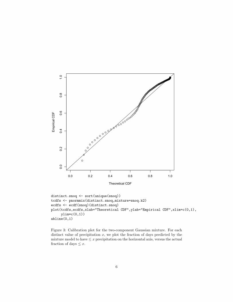
Examining the two-component mixture, it does not look altogether satisfactory— it seems to consistently give too much probability to days with about 1 inchof precipitation. Let’s think about how we could check things like this.

When we looked at logistic regression, we saw how to check probabilityforecasts by checking calibration — events predicted to happen with probabilityp should in fact happen with frequency ≈ p. Here we don’t have a binaryevent, but we do have lots of probabilities. In particular, we have a cumulativedistribution function F (x), which tells us the probability that the precipitationis≤ x on any given day. When x is continuous and has a continuous distribution,F (x) should be uniformly distributed.1 The CDF of a two-component mixtureis

F (x) = λ1F1(x) + λ2F2(x) (1)

and similarly for more components. A little R experimentation gives a functionfor computing the CDF of a Gaussian mixture:

pnormmix <- function(x,mixture) {lambda <- mixture$lambdak <- length(lambda)pnorm.from.mix <- function(x,component) {lambda[component]*pnorm(x,mean=mixture$mu[component],

sd=mixture$sigma[component])}pnorms <- sapply(1:k,pnorm.from.mix,x=x)return(rowSums(pnorms))

}

and so produce a plot like Figure 1.2. We do not have the tools to assess whetherthe size of the departure from the main diagonal is significant2, but the fact thatthe errors are so very structured is rather suspicious.

1We saw this principle when we looked at generating random variables in lecture 7.2Though we could: the most straight-forward thing to do would be to simulate from the

mixture, and repeat this with simulation output.

5

0.0 0.2 0.4 0.6 0.8 1.0

0.0

0.2

0.4

0.6

0.8

1.0

Theoretical CDF

Em

piric

al C

DF

distinct.snoq <- sort(unique(snoq))tcdfs <- pnormmix(distinct.snoq,mixture=snoq.k2)ecdfs <- ecdf(snoq)(distinct.snoq)plot(tcdfs,ecdfs,xlab="Theoretical CDF",ylab="Empirical CDF",xlim=c(0,1),

ylim=c(0,1))abline(0,1)

Figure 3: Calibration plot for the two-component Gaussian mixture. For eachdistinct value of precipitation x, we plot the fraction of days predicted by themixture model to have ≤ x precipitation on the horizontal axis, versus the actualfraction of days ≤ x.

6

1.3 Selecting the Number of Components by Cross-Validation

Since a two-component mixture seems iffy, we could consider using more com-ponents. By going to three, four, etc. components, we improve our in-samplelikelihood, but of course expose ourselves to the danger of over-fitting. Somesort of model selection is called for. We could do cross-validation, or we coulddo hypothesis testing. Let’s try cross-validation first.

We can already do fitting, but we need to calculate the log-likelihood on theheld-out data. As usual, let’s write a function; in fact, let’s write two.

dnormalmix <- function(x,mixture,log=FALSE) {lambda <- mixture$lambdak <- length(lambda)# Calculate share of likelihood for all data for one componentlike.component <- function(x,component) {lambda[component]*dnorm(x,mean=mixture$mu[component],

sd=mixture$sigma[component])}# Create array with likelihood shares from all components over all datalikes <- sapply(1:k,like.component,x=x)# Add up contributions from componentsd <- rowSums(likes)if (log) {d <- log(d)

}return(d)

}

loglike.normalmix <- function(x,mixture) {loglike <- dnormalmix(x,mixture,log=TRUE)return(sum(loglike))

}

To check that we haven’t made a big mistake in the coding:

> loglike.normalmix(snoq,mixture=snoq.k2)[1] -32681.2

which matches the log-likelihood reported by summary(snoq.k2). But our func-tion can be used on different data!

We could do five-fold or ten-fold CV, but just to illustrate the approach we’lldo simple data-set splitting, where a randomly-selected half of the data is usedto fit the model, and half to test.

n <- length(snoq)data.points <- 1:ndata.points <- sample(data.points) # Permute randomlytrain <- data.points[1:floor(n/2)] # First random half is training

7

test <- data.points[-(1:floor(n/2))] # 2nd random half is testingcandidate.component.numbers <- 2:10loglikes <- vector(length=1+length(candidate.component.numbers))# k=1 needs special handlingmu<-mean(snoq[train]) # MLE of meansigma <- sd(snoq[train])*sqrt((n-1)/n) # MLE of standard deviationloglikes[1] <- sum(dnorm(snoq[test],mu,sigma,log=TRUE))for (k in candidate.component.numbers) {mixture <- normalmixEM(snoq[train],k=k,maxit=400,epsilon=1e-2)loglikes[k] <- loglike.normalmix(snoq[test],mixture=mixture)

}

When you run this, you will probably see a lot of warning messages saying“One of the variances is going to zero; trying new starting values.” The issueis that we can give any one value of x arbitrarily high likelihood by centeringa Gaussian there and letting its variance shrink towards zero. This is howevergenerally considered unhelpful — it leads towards the pathologies that keep usfrom doing pure maximum likelihood estimation in non-parametric problems(lecture 6) — so when that happens the code recognizes it and starts over.

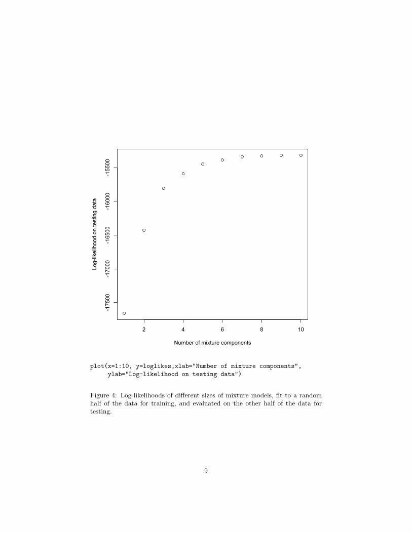
If we look at the log-likelihoods, we see that there is a dramatic improvementwith the first few components, and then things slow down a lot3:

> loglikes[1] -17656.86 -16427.83 -15808.77 -15588.44 -15446.77 -15386.74[7] -15339.25 -15325.63 -15314.22 -15315.88

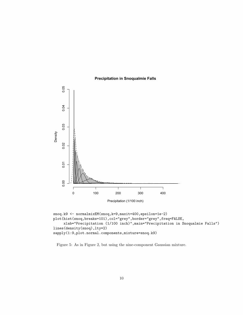
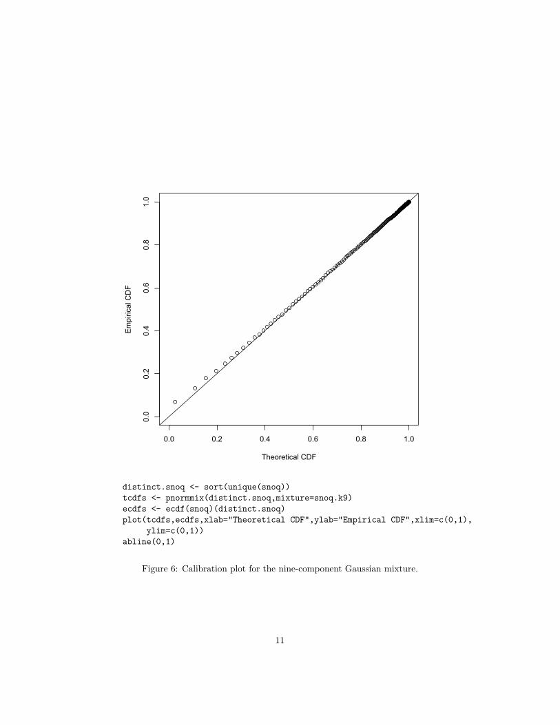
(See also Figure 4). This favors nine components to the mixture. It looks likeFigure 5. The calibration is now nearly perfect, at least on the training data(Figure 1.3).

3Notice that the numbers here are about half of the log-likelihood we calculated for thetwo-component mixture on the complete data. This is as it should be, because log-likelihoodis proportional to the number of observations. (Why?) It’s more like the sum of squarederrors than the mean squared error. If we want something which is directly comparable acrossdata sets of different size, we should use the log-likelihood per observation.

8

2 4 6 8 10

-17500

-17000

-16500

-16000

-15500

Number of mixture components

Log-

likel

ihoo

d on

test

ing

data

plot(x=1:10, y=loglikes,xlab="Number of mixture components",ylab="Log-likelihood on testing data")

Figure 4: Log-likelihoods of different sizes of mixture models, fit to a randomhalf of the data for training, and evaluated on the other half of the data fortesting.

9

Precipitation in Snoqualmie Falls

Precipitation (1/100 inch)

Density

0 100 200 300 400

0.00

0.01

0.02

0.03

0.04

0.05

snoq.k9 <- normalmixEM(snoq,k=9,maxit=400,epsilon=1e-2)plot(hist(snoq,breaks=101),col="grey",border="grey",freq=FALSE,

xlab="Precipitation (1/100 inch)",main="Precipitation in Snoqualmie Falls")lines(density(snoq),lty=2)sapply(1:9,plot.normal.components,mixture=snoq.k9)

Figure 5: As in Figure 2, but using the nine-component Gaussian mixture.

10

0.0 0.2 0.4 0.6 0.8 1.0

0.0

0.2

0.4

0.6

0.8

1.0

Theoretical CDF

Em

piric

al C

DF

distinct.snoq <- sort(unique(snoq))tcdfs <- pnormmix(distinct.snoq,mixture=snoq.k9)ecdfs <- ecdf(snoq)(distinct.snoq)plot(tcdfs,ecdfs,xlab="Theoretical CDF",ylab="Empirical CDF",xlim=c(0,1),

ylim=c(0,1))abline(0,1)

Figure 6: Calibration plot for the nine-component Gaussian mixture.

11

1.4 Interpreting the Mixture Components, or Not

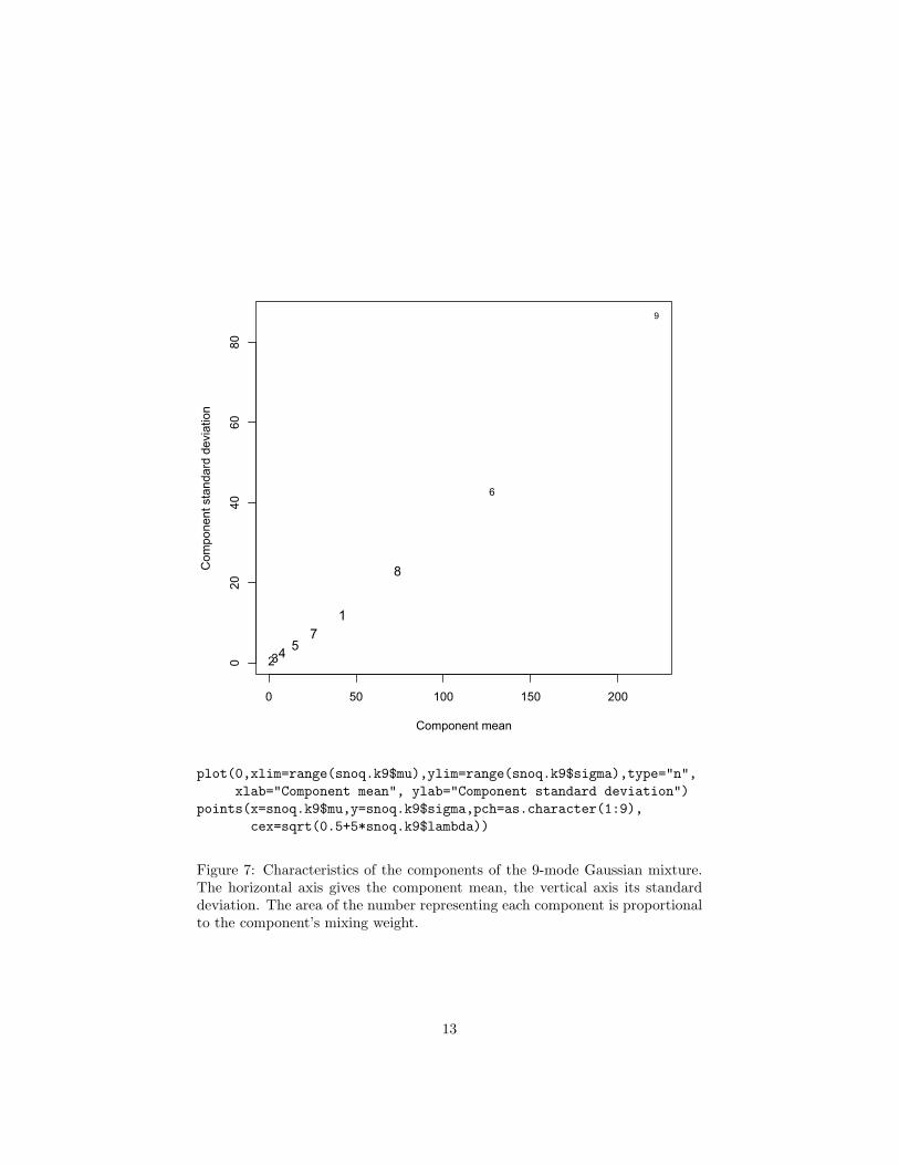
The components of the mixture are far from arbitrary. It appears from Figure5 that as the mean increases, so does the variance. This impression is con-firmed from Figure 7. Now it could be that there really are nine types of rainydays in Snoqualmie Falls which just so happen to have this pattern of distribu-tions, but this seems a bit suspicious — as though the mixture is trying to useGaussians systematically to approximate a fundamentally different distribution,rather than get at something which really is composed of nine distinct Gaus-sians. This judgment relies on our scientific understanding of the weather, whichmakes us surprised by seeing a pattern like this in the parameters. (Calling this“scientific knowledge” is a bit excessive, but you get the idea.) Of course we aresometimes wrong about things like this, so it is certainly not conclusive. Maybethere really are nine types of days, each with a Gaussian distribution, and somesubtle meteorological reason why their means and variances should be linkedlike this. For that matter, maybe our understanding of meteorology is wrong.

There are two directions to take this: the purely statistical one, and thesubstantive one.

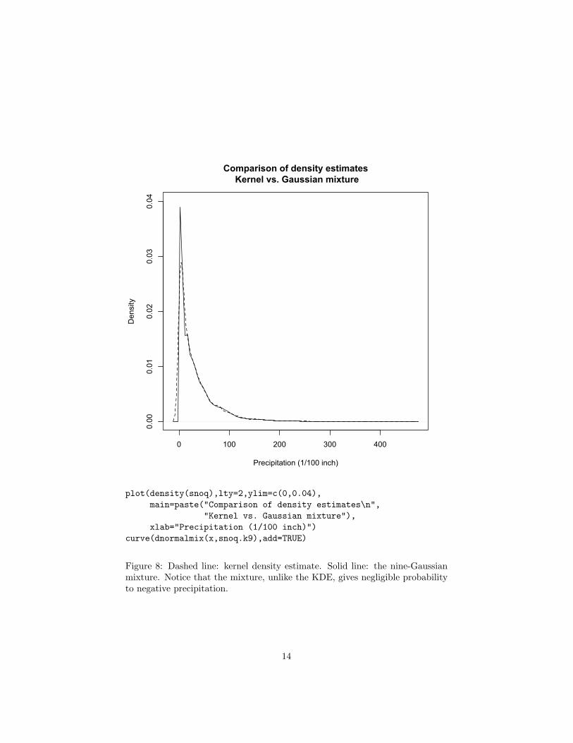
On the purely statistical side, if all we care about is being able to describe thedistribution of the data and to predict future precipitation, then it doesn’t reallymatter whether the nine-component Gaussian mixture is true in any ultimatesense. Cross-validation picked nine components not because there really arenine types of days, but because a nine-component model had the best trade-off between approximation bias and estimation variance. The selected mixturegives a pretty good account of itself, nearly the same as the kernel densityestimate (Figure 8). It requires 26 parameters4, which may seem like a lot, butthe kernel density estimate requires keeping around all 6920 data points plus abandwidth. On sheer economy, the mixture then has a lot to recommend it.

On the substantive side, there are various things we could do to check theidea that wet days really do divide into nine types. These are going to beinformed by our background knowledge about the weather. One of the thingswe know, for example, is that weather patterns more or less repeat in an annualcycle, and that different types of weather are more common in some parts of theyear than in others. If, for example, we consistently find type 6 days in August,that suggests that is at least compatible with these being real, meteorologicalpatterns, and not just approximation artifacts.

Let’s try to look into this visually. snoq.k9$posterior is a 6920× 9 arraywhich gives the probability for each day to belong to each class. I’ll boil thisdown to assigning each day to its most probable class:

day.classes <- apply(snoq.k9$posterior,1,which.max)

We can’t just plot this and hope to see any useful patterns, because we want tosee stuff recurring every year, and we’ve stripped out the dry days, the division

4A mean and a standard deviation for each of nine components (=18 parameters), plusmixing weights (nine of them, but they have to add up to one).

12

0 50 100 150 200

020

4060

80

Component mean

Com

pone

nt s

tand

ard

devi

atio

n

1

2345

6

7

8

9

plot(0,xlim=range(snoq.k9$mu),ylim=range(snoq.k9$sigma),type="n",xlab="Component mean", ylab="Component standard deviation")

points(x=snoq.k9$mu,y=snoq.k9$sigma,pch=as.character(1:9),cex=sqrt(0.5+5*snoq.k9$lambda))

Figure 7: Characteristics of the components of the 9-mode Gaussian mixture.The horizontal axis gives the component mean, the vertical axis its standarddeviation. The area of the number representing each component is proportionalto the component’s mixing weight.

13

0 100 200 300 400

0.00

0.01

0.02

0.03

0.04

Comparison of density estimates Kernel vs. Gaussian mixture

Precipitation (1/100 inch)

Density

plot(density(snoq),lty=2,ylim=c(0,0.04),main=paste("Comparison of density estimates\n",

"Kernel vs. Gaussian mixture"),xlab="Precipitation (1/100 inch)")

curve(dnormalmix(x,snoq.k9),add=TRUE)

Figure 8: Dashed line: kernel density estimate. Solid line: the nine-Gaussianmixture. Notice that the mixture, unlike the KDE, gives negligible probabilityto negative precipitation.

14

into years, the padding to handle leap-days, etc. Fortunately, snoqualmie hasall that, so we’ll make a copy of that and edit day.classes into it.

snoqualmie.classes <- snoqualmiewet.days <- (snoqualmie > 0) & !(is.na(snoqualmie))snoqualmie.classes[wet.days] <- day.classes

(Note that wet.days is a 36 × 366 logical array.) Now, it’s somewhat incon-venient that the index numbers of the components do not perfectly correspondto the mean amount of precipitation — class 9 really is more similar to class6 than to class 8. (See Figure 7.) Let’s try replacing the numerical labels insnoqualmie.classes by those means.

snoqualmie.classes[wet.days] <- snoq.k9$mu[day.classes]

This leaves alone dry days (still zero) and NA days (still NA). Now we can plot(Figure 9).

The result is discouraging if we want to read any deeper meaning into theclasses. The class with the heaviest amounts of precipitation is most common inthe winter, but so is the classes with the second-heaviest amount of precipitation,the etc. It looks like the weather changes smoothly, rather than really havingdiscrete classes. In this case, the mixture model seems to be merely a predictivedevice, and not a revelation of hidden structure.5

5A a distribution called a “type II generalized Pareto”, where p(x) ∝ (1 + x/σ)−θ−1, pro-vides a decent fit here. (See Shalizi 2007; Arnold 1983 on this distribution and its estimation.)With only two parameters, rather than 26, its log-likelihood is only 1% higher than that ofthe nine-component mixture, and it is almost but not quite as calibrated. One origin of thetype II Pareto is as a mixture of exponentials (Maguire et al., 1952). If X|Z ∼ Exp(σ/Z),and Z itself has a Gamma distribution, Z ∼ Γ(θ, 1), then the unconditional distribution ofX is type II Pareto with scale σ and shape θ. We might therefore investigate fitting a finitemixture of exponentials, rather than of Gaussians, for the Snoqualmie Falls data. We mightof course still end up concluding that there is a continuum of different sorts of days, ratherthan a finite set of discrete types.

15

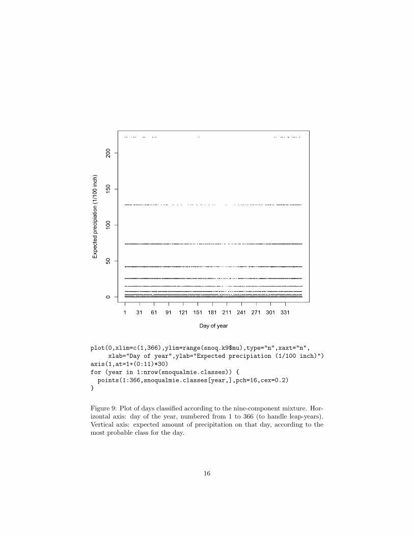
plot(0,xlim=c(1,366),ylim=range(snoq.k9$mu),type="n",xaxt="n",xlab="Day of year",ylab="Expected precipiation (1/100 inch)")

axis(1,at=1+(0:11)*30)for (year in 1:nrow(snoqualmie.classes)) {points(1:366,snoqualmie.classes[year,],pch=16,cex=0.2)

}

Figure 9: Plot of days classified according to the nine-component mixture. Hor-izontal axis: day of the year, numbered from 1 to 366 (to handle leap-years).Vertical axis: expected amount of precipitation on that day, according to themost probable class for the day.

16

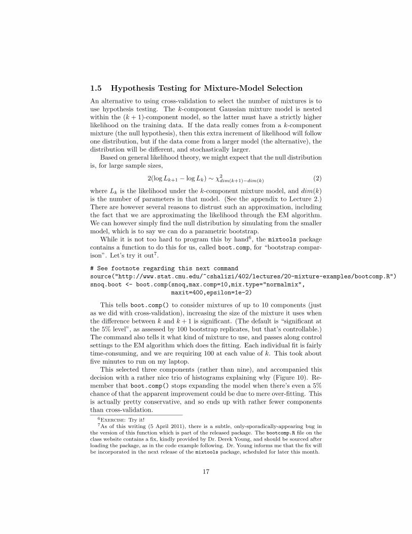
1.5 Hypothesis Testing for Mixture-Model Selection

An alternative to using cross-validation to select the number of mixtures is touse hypothesis testing. The k-component Gaussian mixture model is nestedwithin the (k + 1)-component model, so the latter must have a strictly higherlikelihood on the training data. If the data really comes from a k-componentmixture (the null hypothesis), then this extra increment of likelihood will followone distribution, but if the data come from a larger model (the alternative), thedistribution will be different, and stochastically larger.

Based on general likelihood theory, we might expect that the null distributionis, for large sample sizes,

2(logLk+1 − logLk) ∼ χ2dim(k+1)−dim(k) (2)

where Lk is the likelihood under the k-component mixture model, and dim(k)is the number of parameters in that model. (See the appendix to Lecture 2.)There are however several reasons to distrust such an approximation, includingthe fact that we are approximating the likelihood through the EM algorithm.We can however simply find the null distribution by simulating from the smallermodel, which is to say we can do a parametric bootstrap.

While it is not too hard to program this by hand6, the mixtools packagecontains a function to do this for us, called boot.comp, for “bootstrap compar-ison”. Let’s try it out7.

# See footnote regarding this next commandsource("http://www.stat.cmu.edu/~cshalizi/402/lectures/20-mixture-examples/bootcomp.R")snoq.boot <- boot.comp(snoq,max.comp=10,mix.type="normalmix",

maxit=400,epsilon=1e-2)

This tells boot.comp() to consider mixtures of up to 10 components (justas we did with cross-validation), increasing the size of the mixture it uses whenthe difference between k and k + 1 is significant. (The default is “significant atthe 5% level”, as assessed by 100 bootstrap replicates, but that’s controllable.)The command also tells it what kind of mixture to use, and passes along controlsettings to the EM algorithm which does the fitting. Each individual fit is fairlytime-consuming, and we are requiring 100 at each value of k. This took aboutfive minutes to run on my laptop.

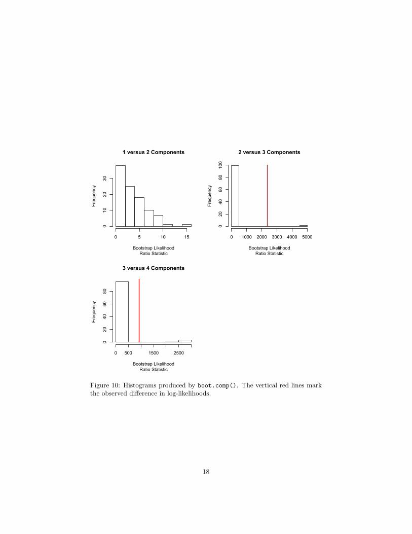
This selected three components (rather than nine), and accompanied thisdecision with a rather nice trio of histograms explaining why (Figure 10). Re-member that boot.comp() stops expanding the model when there’s even a 5%chance of that the apparent improvement could be due to mere over-fitting. Thisis actually pretty conservative, and so ends up with rather fewer componentsthan cross-validation.

6Exercise: Try it!7As of this writing (5 April 2011), there is a subtle, only-sporadically-appearing bug in

the version of this function which is part of the released package. The bootcomp.R file on theclass website contains a fix, kindly provided by Dr. Derek Young, and should be sourced afterloading the package, as in the code example following. Dr. Young informs me that the fix willbe incorporated in the next release of the mixtools package, scheduled for later this month.

17

1 versus 2 Components

Bootstrap LikelihoodRatio Statistic

Frequency

0 5 10 15

010

2030

2 versus 3 Components

Bootstrap LikelihoodRatio Statistic

Frequency

0 1000 2000 3000 4000 5000

020

4060

80100

3 versus 4 Components

Bootstrap LikelihoodRatio Statistic

Frequency

0 500 1500 2500

020

4060

80

Figure 10: Histograms produced by boot.comp(). The vertical red lines markthe observed difference in log-likelihoods.

18

Let’s explore the output of boot.comp(), conveniently stored in the objectsnoq.boot.

> str(snoq.boot)List of 3$ p.values : num [1:3] 0 0.01 0.05$ log.lik :List of 3..$ : num [1:100] 5.889 1.682 9.174 0.934 4.682 .....$ : num [1:100] 2.434 0.813 3.745 6.043 1.208 .....$ : num [1:100] 0.693 1.418 2.372 1.668 4.084 ...$ obs.log.lik: num [1:3] 5096 2354 920

This tells us that snoq.boot is a list with three elements, called p.values,log.lik and obs.log.lik, and tells us a bit about each of them. p.valuescontains the p-values for testing H1 (one component) against H2 (two compo-nents), testing H2 against H3, and H3 against H4. Since we set a thresholdp-value of 0.05, it stopped at the last test, accepting H3. (Under these circum-stances, if the difference between k = 3 and k = 4 was really important to us, itwould probably be wise to increase the number of bootstrap replicates, to getmore accurate p-values.) log.lik is itself a list containing the bootstrappedlog-likelihood ratios for the three hypothesis tests; obs.log.lik is the vector ofcorresponding observed values of the test statistic.

Looking back to Figure 4, there is indeed a dramatic improvement in thegeneralization ability of the model going from one component to two, and fromtwo to three, and diminishing returns to complexity thereafter. Stopping atk = 3 produces pretty reasonable results, though repeating the exercise of Figure9 is no more encouraging for the reality of the latent classes.

19

2 Multivariate Gaussians

Most of this section repeats the appendix to Lecture 4.

The multivariate Gaussian is just the generalization of the ordinary Gaussianto vectors. Scalar Gaussians are parameterized by a mean µ and a variance σ2,which we symbolize by writing X ∼ N (µ, σ2). Multivariate Gaussians, likewise,are parameterized by a mean vector ~µ, and a variance-covariance matrix Σ,written ~X ∼MVN (~µ,Σ). The components of ~µ are the means of the differentcomponents of ~X. The i, jth component of Σ is the covariance between Xi andXj (so the diagonal of Σ gives the component variances).

Just as the probability density of scalar Gaussian is

p(x) =(2πσ2

)−1/2exp

{−1

2(x− µ)2

σ2

}(3)

the probability density of the multivariate Gaussian is

p(~x) = (2π det Σ)−d/2 exp{−1

2(~x− ~µ) ·Σ−1(~x− ~µ)

}(4)

Finally, remember that the parameters of a Gaussian change along with lineartransformations

X ∼ N (µ, σ2)⇔ aX + b ∼ N (aµ+ b, a2σ2) (5)

and we can use this to “standardize” any Gaussian to having mean 0 and vari-ance 1 (by looking at X−µ

σ ). Likewise, if

~X ∼MVN (~µ,Σ) (6)

thena ~X +~b ∼MVN (a~µ+~b,aΣaT ) (7)

In fact, the analogy between the ordinary and the multivariate Gaussian is socomplete that it is very common to not really distinguish the two, and write Nfor both.

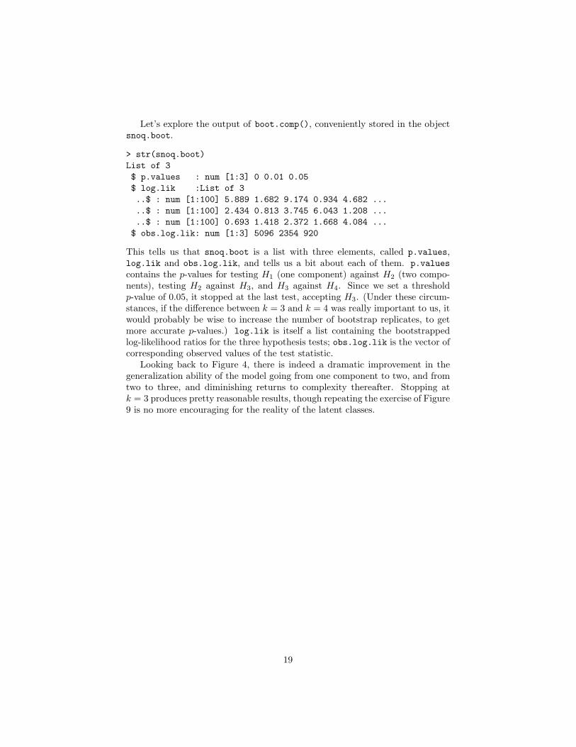
The multivariate Gaussian density is most easily visualized when d = 2,as in Figure 11. The probability contours are ellipses. The density changescomparatively slowly along the major axis, and quickly along the minor axis.The two points marked + in the figure have equal geometric distance from ~µ,but the one to its right lies on a higher probability contour than the one aboveit, because of the directions of their displacements from the mean.

In fact, we can use some facts from linear algebra to understand the generalpattern here, for arbitrary multivariate Gaussians in an arbitrary number ofdimensions. The covariance matrix Σ is symmetric and positive-definite, so weknow from matrix algebra that it can be written in terms of its eigenvalues andeigenvectors:

Σ = vTdv (8)

20

-3 -2 -1 0 1 2 3

-3-2

-10

12

3

+

+

library(mvtnorm)x.points <- seq(-3,3,length.out=100)y.points <- x.pointsz <- matrix(0,nrow=100,ncol=100)mu <- c(1,1)sigma <- matrix(c(2,1,1,1),nrow=2)for (i in 1:100) {for (j in 1:100) {

z[i,j] <- dmvnorm(c(x.points[i],y.points[j]),mean=mu,sigma=sigma)}

}contour(x.points,y.points,z)

Figure 11: Probability density contours for a two-dimensional multivariate

Gaussian, with mean ~µ =(

11

)(solid dot), and variance matrix Σ =(

2 11 1

). Using expand.grid, as in Lecture 6, would be more elegant coding

than this double for loop.21

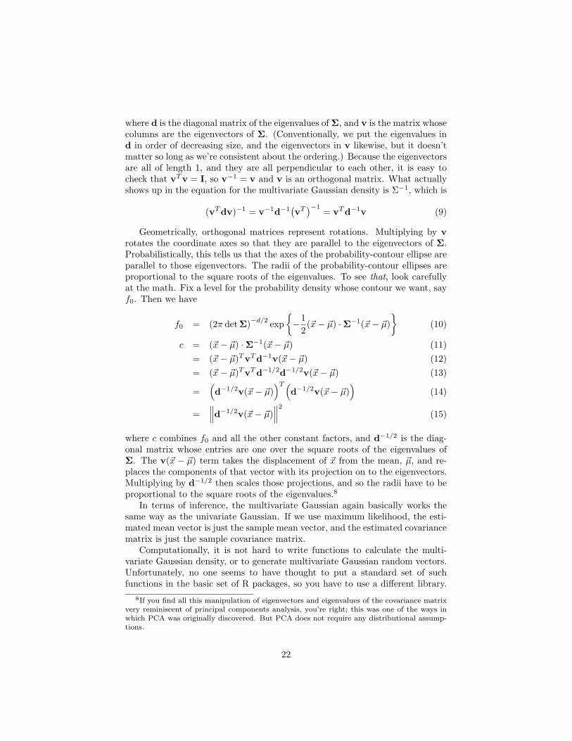
where d is the diagonal matrix of the eigenvalues of Σ, and v is the matrix whosecolumns are the eigenvectors of Σ. (Conventionally, we put the eigenvalues ind in order of decreasing size, and the eigenvectors in v likewise, but it doesn’tmatter so long as we’re consistent about the ordering.) Because the eigenvectorsare all of length 1, and they are all perpendicular to each other, it is easy tocheck that vTv = I, so v−1 = v and v is an orthogonal matrix. What actuallyshows up in the equation for the multivariate Gaussian density is Σ−1, which is

(vTdv)−1 = v−1d−1(vT

)−1= vTd−1v (9)

Geometrically, orthogonal matrices represent rotations. Multiplying by vrotates the coordinate axes so that they are parallel to the eigenvectors of Σ.Probabilistically, this tells us that the axes of the probability-contour ellipse areparallel to those eigenvectors. The radii of the probability-contour ellipses areproportional to the square roots of the eigenvalues. To see that, look carefullyat the math. Fix a level for the probability density whose contour we want, sayf0. Then we have

f0 = (2π det Σ)−d/2 exp{−1

2(~x− ~µ) ·Σ−1(~x− ~µ)

}(10)

c = (~x− ~µ) ·Σ−1(~x− ~µ) (11)= (~x− ~µ)TvTd−1v(~x− ~µ) (12)= (~x− ~µ)TvTd−1/2d−1/2v(~x− ~µ) (13)

=(d−1/2v(~x− ~µ)

)T(d−1/2v(~x− ~µ)

)(14)

=∥∥∥d−1/2v(~x− ~µ)

∥∥∥2

(15)

where c combines f0 and all the other constant factors, and d−1/2 is the diag-onal matrix whose entries are one over the square roots of the eigenvalues ofΣ. The v(~x − ~µ) term takes the displacement of ~x from the mean, ~µ, and re-places the components of that vector with its projection on to the eigenvectors.Multiplying by d−1/2 then scales those projections, and so the radii have to beproportional to the square roots of the eigenvalues.8

In terms of inference, the multivariate Gaussian again basically works thesame way as the univariate Gaussian. If we use maximum likelihood, the esti-mated mean vector is just the sample mean vector, and the estimated covariancematrix is just the sample covariance matrix.

Computationally, it is not hard to write functions to calculate the multi-variate Gaussian density, or to generate multivariate Gaussian random vectors.Unfortunately, no one seems to have thought to put a standard set of suchfunctions in the basic set of R packages, so you have to use a different library.

8If you find all this manipulation of eigenvectors and eigenvalues of the covariance matrixvery reminiscent of principal components analysis, you’re right; this was one of the ways inwhich PCA was originally discovered. But PCA does not require any distributional assump-tions.

22

mvtnorm contains functions for calculating the density, cumulative distributionand quantiles of the multivariate Gaussian, and for generating random vectors9

The package mixtools, which we are using for mixture models, includes func-tions for the multivariate Gaussian density and for random-vector generation.

3 Exercises

Not to be handed in.

1. Write a function to calculate the density of a multivariate Gaussian witha given mean vector and covariance matrix. Check it against an existingfunction from one of the packages mentioned above.

2. Write a function to generate multivariate Gaussian random vectors, usingrnorm.

3. Write a function to simulate from a Gaussian mixture model.

4. Write a function to fit a mixture of exponential distributions using theEM algorithm. Does it do any better at discovering sensible structure inthe Snoqualmie Falls data?

References

Arnold, Barry C. (1983). Pareto Distributions. Fairland, Maryland: Interna-tional Cooperative Publishing House.

Maguire, B. A., E. S. Pearson and A. H. A. Wynn (1952). “The time intervalsbetween industrial accidents.” Biometrika, 39: 168–180. URL http://www.jstor.org/pss/2332475.

Shalizi, Cosma Rohilla (2007). “Maximum Likelihood Estimation and ModelTesting for q-Exponential Distributions.” Physical Review E , submitted.URL http://arxiv.org/abs/math.ST/0701854.

9It also has such functions for multivariate t distributions, which are to multivariate Gaus-sians exactly as ordinary t distributions are to univariate Gaussians.

23