Learning Embeddings for Similarity-Based Retrieval

1

Learning Embeddings for Similarity-Based Retrieval

Vassilis Athitsos

Computer Science Department

Boston University

2

Overview

Background on similarity-based retrieval and embeddings.

BoostMap. Embedding optimization using machine learning.

Query-sensitive embeddings. Ability to preserve non-metric structure.

3

database(n objects)

x1

x2

x3

xn

Problem Definition

4

database(n objects)

x1

x2

x3

xn

q

Problem Definition

Goals: find the k nearest neighbors of

query q.

5


query q.

Brute force time is linear to: n (size of database). time it takes to measure a

single distance.

database(n objects)

x1

x2

x3

xn

q

Problem Definition

x2

xn

6


query q.

Brute force time is linear to: n (size of database). time it takes to measure a

single distance.

database(n objects)

x1

x3q

Problem Definition

x2

xn

7

Applications Nearest neighbor

classification.

Similarity-based retrieval. Image/video databases. Biological databases. Time series. Web pages. Browsing music or movie

catalogs.faces

letters/digits

handshapes

8

Expensive Distance Measures

Comparing d-dimensional vectors is efficient: O(d) time.

x1 x2 x3 x4 … xd

y1 y2 y3 y4 … yd

9



Comparing strings of length d with the edit distance is more expensive: O(d2) time.

Reason: alignment.x1 x2 x3 x4 … xd

y1 y2 y3 y4 … yd

i m m i g r a t i o n

i m i t a t i o n

10



Comparing strings of length d with the edit distance is more expensive: O(d2) time.

Reason: alignment.x1 x2 x3 x4 … xd

y1 y2 y3 y4 … yd

i m m i g r a t i o n

i m i t a t i o n

11

Matching Handwritten Digits

12


13


14

Shape Context Distance

Proposed by Belongie et al. (2001). Error rate: 0.63%, with database of 20,000 images. Uses bipartite matching (cubic complexity!). 22 minutes/object, heavily optimized. Result preview: 5.2 seconds, 0.61% error rate.

15

More Examples

DNA and protein sequences: Smith-Waterman.

Time series: Dynamic Time Warping.

Probability distributions: Kullback-Leibler Distance.

These measures are non-Euclidean, sometimes non-metric.

16

Indexing Problem

Vector indexing methods NOT applicable. PCA. R-trees, X-trees, SS-trees. VA-files. Locality Sensitive Hashing.

17

Metric Methods Pruning-based methods.

VP-trees, MVP-trees, M-trees, Slim-trees,… Use triangle inequality for tree-based search.

Filtering methods. AESA, LAESA… Use the triangle inequality to compute upper/lower

bounds of distances.

Suffer from curse of dimensionality. Heuristic in non-metric spaces. In many datasets, bad empirical performance.

18

Embeddings

database

x1

x2

x3

xn

embedding F

x1x2

x3

x4

xn

Rd

19

Embeddings

database

x1

x2

x3

xn

embedding F

x1x2

x3

x4

xn

q

query

Rd

20

Embeddings

database

x1

x2

x3

xn

embedding F

x1x2

x3

x4

xn

q

query

q

Rd

21

Embeddings

database

x1

x2

x3

xn

embedding F

x1x2

x3

x4

xn

Rd

q

query

q

Measure distances between vectors (typically much faster).

22

Embeddings

database

x1

x2

x3

xn

embedding F

x1x2

x3

x4

xn

Rd

q

query

q

Measure distances between vectors (typically much faster).

Caveat: the embedding must preserve similarity structure.

23

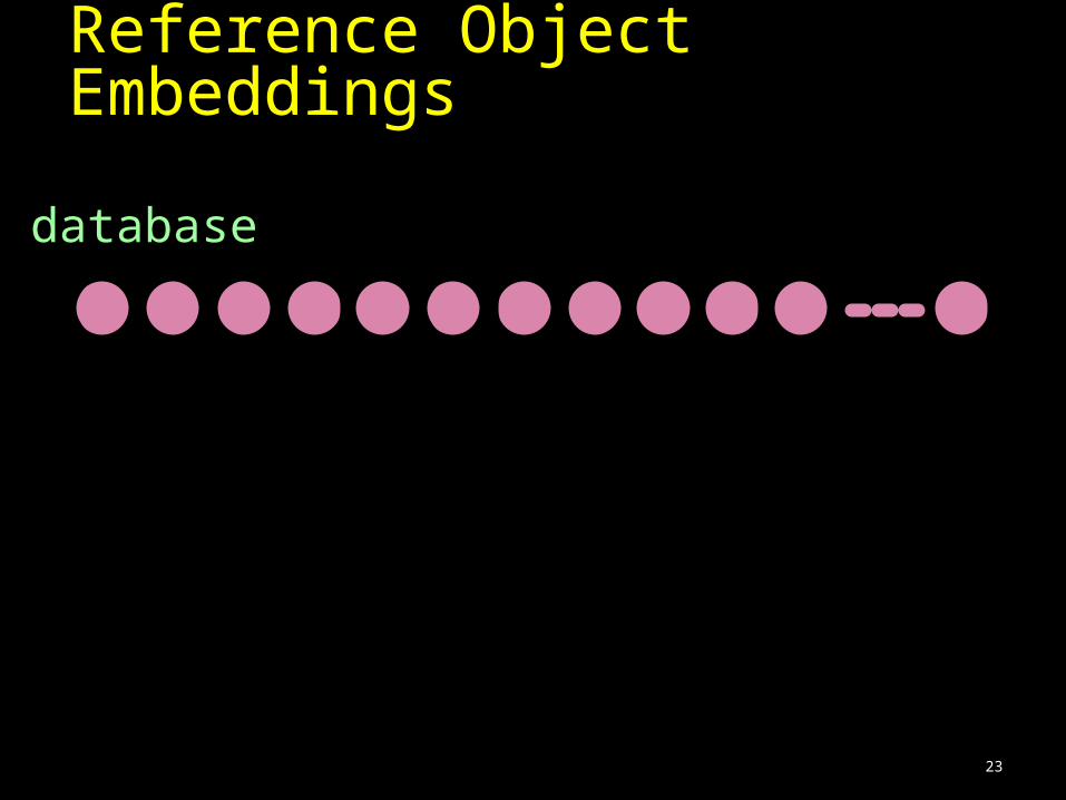
Reference Object Embeddings

database

24


databaser1 r2 r3

25


databaser1 r2 r3

x

F(x) = (D(x, r1), D(x, r2), D(x, r3))

26

F(x) = (D(x, LA), D(x, Lincoln), D(x, Orlando))

F(Sacramento)....= ( 386, 1543, 2920)F(Las Vegas).....= ( 262, 1232, 2405)F(Oklahoma City).= (1345, 437, 1291)F(Washington DC).= (2657, 1207, 853)F(Jacksonville)..= (2422, 1344, 141)

27

Existing Embedding Methods FastMap, MetricMap, SparseMap, Lipschitz

embeddings. Use distances to reference objects (prototypes).

Question: how do we directly optimize an embedding for nearest neighbor retrieval? FastMap & MetricMap assume Euclidean

properties. SparseMap optimizes stress.

Large stress may be inevitable when embedding non-metric spaces into a metric space.

In practice often worse than random construction.

28

BoostMap

BoostMap: A Method for Efficient Approximate Similarity Rankings.Athitsos, Alon, Sclaroff, and Kollios,CVPR 2004.

BoostMap: An Embedding Method for Efficient Nearest Neighbor Retrieval. Athitsos, Alon, Sclaroff, and Kollios,PAMI 2007 (to appear).

29

Key Features of BoostMap

Maximizes amount of nearest neighbor structure preserved by the embedding.

Based on machine learning, not on geometric assumptions. Principled optimization, even in non-metric spaces.

Can capture non-metric structure. Query-sensitive version of BoostMap.

Better results in practice, in all datasets we have tried.

30

Ideal Embedding Behavior

original space X F Rd

aq

For any query q: we want F(NN(q)) = NN(F(q)).

31



aq


32




aq

33



aq


For any database object b besides NN(q), we want F(q) closer to F(NN(q)) than to F(b).

b

34

Embeddings Seen As Classifiers

qa

b For triples (q, a, b) such that:- q is a query object- a = NN(q)- b is a database object

Classification task: is qcloser to a or to b?

35

Any embedding F defines a classifier F’(q, a, b). F’ checks if F(q) is closer to F(a) or to F(b).

qa

b

Embeddings Seen As Classifiers

For triples (q, a, b) such that:- q is a query object- a = NN(q)- b is a database object


36

Given embedding F: X Rd: F’(q, a, b) = ||F(q) – F(b)|| - ||F(q) – F(a)||.

F’(q, a, b) > 0 means “q is closer to a.” F’(q, a, b) < 0 means “q is closer to b.”

qa

b

Classifier Definition

For triples (q, a, b) such that:- q is a query object- a = NN(q)- b is a database object


37

Key Observation


aq

b

If classifier F’ is perfect, then for every q, F(NN(q)) = NN(F(q)). If F(q) is closer to F(b) than to F(NN(q)), then triple

(q, a, b) is misclassified.

38

Key Observation


aq

b

Classification error on triples (q, NN(q), b) measures how well F preserves nearest neighbor structure.

39

Goal: construct an embedding F optimized for k-nearest neighbor retrieval.

Method: maximize accuracy of F’ on triples (q, a, b) of the following type: q is any object. a is a k-nearest neighbor of q in the database. b is in database, but NOT a k-nearest neighbor of q.

If F’ is perfect on those triples, then F perfectly preserves k-nearest neighbors.

Optimization Criterion

40

1D Embeddings as Weak Classifiers 1D embeddings define weak classifiers.

Better than a random classifier (50% error rate).

41

Lincoln

Chicago

Detroit

New York

LA

Cleveland

Detroit New York

Chicago LA

42



We can define lots of different classifiers. Every object in the database can be a reference object.

43




Question: how do we combine many such

classifiers into a single strong classifier?

44




Question: how do we combine many such

classifiers into a single strong classifier?

Answer: use AdaBoost. AdaBoost is a machine learning method designed for

exactly this problem.

45

Using AdaBoostoriginal space X

Fn

F2

F1

Real line

Output: H = w1F’1 + w2F’2 + … + wdF’d . AdaBoost chooses 1D embeddings and weighs them. Goal: achieve low classification error. AdaBoost trains on triples chosen from the database.

46

From Classifier to Embedding

AdaBoost output H = w1F’1 + w2F’2 + … + wdF’d

What embedding should we use?What distance measure should we use?

47



F(x) = (F1(x), …, Fd(x)).BoostMap embedding

48



D((u1, …, ud), (v1, …, vd)) = i=1 wi|ui – vi|

d


Distance measure

49



D((u1, …, ud), (v1, …, vd)) = i=1 wi|ui – vi|

d


Distance measure

Claim: Let q be closer to a than to b. H misclassifiestriple (q, a, b) if and only if, under distance measure D, F maps q closer to b than to a.

50

Proof

H(q, a, b) =

= wiF’i(q, a, b)

= wi(|Fi(q) - Fi(b)| - |Fi(q) - Fi(a)|)

= (wi|Fi(q) - Fi(b)| - wi|Fi(q) - Fi(a)|)

= D(F(q), F(b)) – D(F(q), F(a)) = F’(q, a, b)

i=1

d

i=1

d

i=1

d

51

Proof

H(q, a, b) =

= wiF’i(q, a, b)

= wi(|Fi(q) - Fi(b)| - |Fi(q) - Fi(a)|)


= D(F(q), F(b)) – D(F(q), F(a)) = F’(q, a, b)

i=1

d

i=1

d

i=1

d

52

Proof

H(q, a, b) =

= wiF’i(q, a, b)

= wi(|Fi(q) - Fi(b)| - |Fi(q) - Fi(a)|)


= D(F(q), F(b)) – D(F(q), F(a)) = F’(q, a, b)

i=1

d

i=1

d

i=1

d

53

Proof

H(q, a, b) =

= wiF’i(q, a, b)

= wi(|Fi(q) - Fi(b)| - |Fi(q) - Fi(a)|)


= D(F(q), F(b)) – D(F(q), F(a)) = F’(q, a, b)

i=1

d

i=1

d

i=1

d

54

Proof

H(q, a, b) =

= wiF’i(q, a, b)

= wi(|Fi(q) - Fi(b)| - |Fi(q) - Fi(a)|)


= D(F(q), F(b)) – D(F(q), F(a)) = F’(q, a, b)

i=1

d

i=1

d

i=1

d

55

Proof

H(q, a, b) =

= wiF’i(q, a, b)

= wi(|Fi(q) - Fi(b)| - |Fi(q) - Fi(a)|)


= D(F(q), F(b)) – D(F(q), F(a)) = F’(q, a, b)

i=1

d

i=1

d

i=1

d

56

Significance of Proof

AdaBoost optimizes a direct measure of embedding quality.

We optimize an indexing structure for similarity-based retrieval using machine learning. Take advantage of training data.

57

How Do We Use It?

Filter-and-refine retrieval: Offline step: compute embedding F of

entire database.

58

How Do We Use It?


entire database. Given a query object q:

Embedding step: Compute distances from query to reference

objects F(q).

59

How Do We Use It?




objects F(q). Filter step:

Find top p matches of F(q) in vector space.

60

How Do We Use It?





Find top p matches of F(q) in vector space. Refine step:

Measure exact distance from q to top p matches.

61

Evaluating Embedding Quality





How often do we find the true nearest neighbor?

62







63







How many exact distance computations do we need?

64








65








66






What is the nearest neighbor classification error?


67Chamfer distance: 112 seconds per query

Results on Hand Dataset

query

Database (80,640 images)nearest neighbor

68

Query set: 710 real images of hands.

Database: 80,640 synthetic images of hands.


Brute Force

Accuracy 100%

Distances 80640

Seconds 112

Speed-up 1

69

Brute Force

BM RLP FM VP

Accuracy 100% 95% 95% 95% 95%

Distances 80640 450 1444 2647 5471

Seconds 112 0.6 2.0 3.7 7.6

Speed-up 1 179 56 30 15


Query set: 710 real images of hands.

Database: 80,640 synthetic images of hands.

70

MNIST: 60,000 database objects, 10,000 queries. Shape context (Belongie 2001):

0.63% error, 20,000 distances, 22 minutes. 0.54% error, 60,000 distances, 66 minutes.

Results on MNIST Dataset

71

Results on MNIST Dataset

Method Distances per query

Seconds per query

Error rate

Brute force 60,000 3,696 0.54%

VP-trees 21,152 1306 0.63%

Condensing 1,060 71 2.40%

BoostMap 800 53 0.58%

Zhang 2003 50 3.3 2.55%

BoostMap 50 3.3 1.50%

BoostMap* 50 3.3 0.83%

72

Query-Sensitive Embeddings

Richer models. Capture non-metric structure. Better embedding quality.

References: Athitsos, Hadjieleftheriou, Kollios, and Sclaroff,

SIGMOD 2005. Athitsos, Hadjieleftheriou, Kollios, and Sclaroff,

TODS, June 2007.

73

Capturing Non-Metric Structure

A human is not similar to a horse. A centaur is similar both to a human and a horse. Triangle inequality is violated:

Using human ratings of similarity (Tversky, 1982). Using k-median Hausdorff distance.

74

Capturing Non-Metric Structure

Mapping to a metric space presents dilemma: If D(F(centaur), F(human)) = D(F(centaur), F(horse)) = C,

then D(F(human), F(horse)) <= 2C.

Query-sensitive embeddings: Have the modeling power to preserve non-metric structure.

75

Local Importance of Coordinates

How important is each coordinate in comparing embeddings?

databasex1

x2

xn

embedding F

Rd

qquery

x11 x12 x13 x14 … x1d

x21 x22 x23 x24 … x2d

xn1 xn2 xn3 xn4 … xnd

q1 q2 q3 q4 … qd

76



77

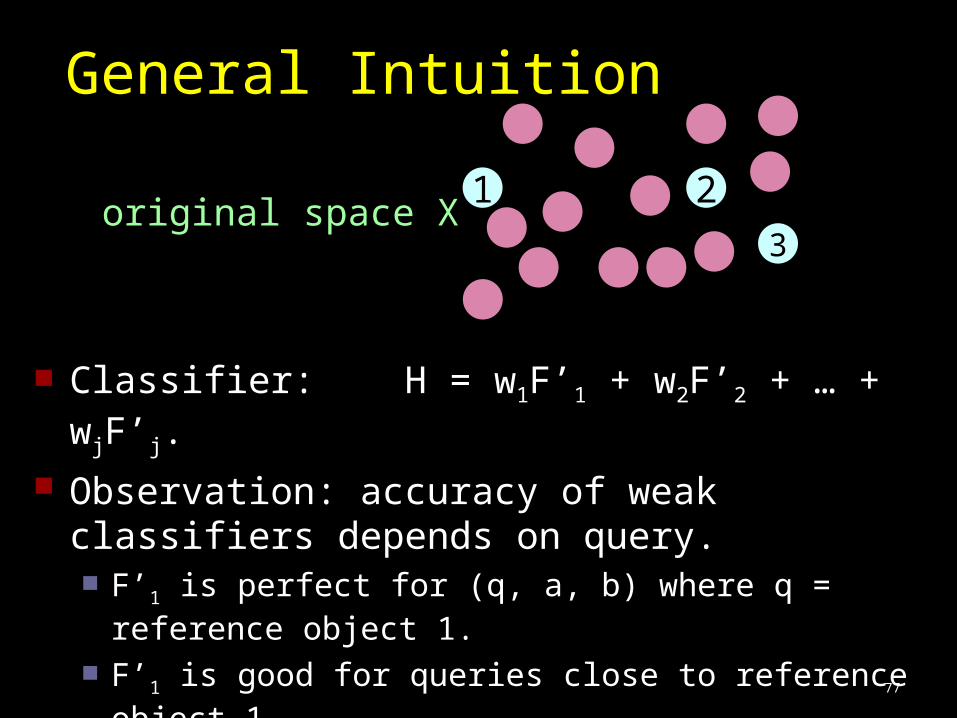
original space X1 2

3

Classifier: H = w1F’1 + w2F’2 + … + wjF’j. Observation: accuracy of weak classifiers depends

on query. F’1 is perfect for (q, a, b) where q = reference object 1.

F’1 is good for queries close to reference object 1.

Question: how can we capture that?

General Intuition

78

Query-Sensitive Weak Classifiers

V: area of influence (interval of real numbers).

F’(q, a, b) if F(q) is in V QF,V(q, a, b) = “I don’t know” if F(q) not in V

original space X1 2

3

79

Query-Sensitive Weak Classifiers

V: area of influence (interval of real numbers).

F’(q, a, b) if F(q) is in V QF,V(q, a, b) = “I don’t know” if F(q) not in V If V includes all real numbers, QF,V = F’.

original space X1 2

j

80

Applying AdaBoost

original space X

Fd

F2

F1

Real line

AdaBoost forms classifiers QFi,Vi.

Fi: 1D embedding.

Vi: area of influence for Fi.

Output: H = w1 QF1,V1 + w2 QF2,V2

+ … + wd QFd,Vd .

81

Applying AdaBoost

original space X

Fd

F2

F1

Real line

Empirical observation: At late stages of the training, query-sensitive weak

classifiers are still useful, whereas query-insensitive classifiers are not.

82


What embedding should we use?What distance measure should we use?

AdaBoost output

H(q, a, b) = i=1 wi QFi,Vi

(q, a, b)d

83


D(F(q), F(x)) = i=1 wi SFi,Vi

(q) |Fi(q) – Fi(x)|

d

F(x) = (F1(x), …, Fd(x))BoostMap embedding

Distance measure

AdaBoost output


(q, a, b)d

84


Distance measure is query-sensitive. Weighted L1 distance, weights depend on q.

SF,V(q) = 1 if F(q) is in V, 0 otherwise.

D(F(q), F(x)) = i=1 wi SFi,Vi

(q) |Fi(q) – Fi(x)|

d

F(x) = (F1(x), …, Fd(x))BoostMap embedding

Distance measure

AdaBoost output


(q, a, b)d

85

Centaurs Revisited

Reference objects: human, horse, centaur. For centaur queries, use weights (0,0,1). For human queries, use weights (1,0,0).

Query-sensitive distances are non-metric. Combine efficiency of L1 distance and ability to capture non-metric

structure.

86



87

Recap of Advantages

Capturing non-metric structure. Finding most informative reference

objects for each query. Richer model overall.

Choosing a weak classifier now also involves choosing an area of influence.

88

Query-Sensitive

Query-Insensitive

Accuracy 95% 95%

# of distances 1995 5691

Sec. per query 33 95

Speed-up factor 16 5.6

Query set: 1000 time series.

Database: 31818 time series.

Dynamic Time Warping on Time Series

89

Query-Sensitive

Vlachos KDD 2003

Accuracy 100% 100%

# of distances 640 over 6500

Sec. per query 10.7 over 110

Speed-up factor 51.2 under 5

Query set: 50 time series.

Database: 32768 time series.

Dynamic Time Warping on Time Series

90

BoostMap Recap - Theory

Machine-learning method for optimizing embeddings. Explicitly maximizes amount of nearest neighbor

structure preserved by embedding. Optimization method is independent of underlying

geometry. Query-sensitive version can capture non-metric

structure.

91

BoostMap Recap - Practice

BoostMap can significantly speed up nearest neighbor retrieval and classification. Useful in real-world datasets:

Hand shape classification. Optical character recognition (MNIST, UNIPEN).

In all four datasets, better results than other methods. In three benchmark datasets, better than methods

custom-made for those distance measures. Domain-independent formulation.

Distance measures are used as a black box. Application to proteins/DNA matching…

92

END

Documents

Learning Embeddings for Similarity-Based Retrieval