Document Similarity in Information Retrieval · Document Similarity in Information Retrieval Mausam (Based on slides of W. Arms, Thomas Hofmann, Ata Kaban, Melanie Martin)

Document Similarity in

Information Retrieval

Mausam

(Based on slides of W. Arms, Thomas

Hofmann, Ata Kaban, Melanie Martin)

Standard Web Search Engine Architecture

crawl the

web

create an

inverted

index

store documents, check for duplicates,

extract links

inverted

index

DocIds

Slide adapted from Marti Hearst / UC Berkeley]

Search

engine

servers

user

query

show results

To user

Indexing Subsystem

Documents

break into tokens

stop list*

stemming*

term weighting*

Index

database

text

non-stoplist

tokens

tokens

stemmed

terms

terms with

weights

*Indicates

optional

operation.

assign document IDs documents

document

numbers

and *field

numbers

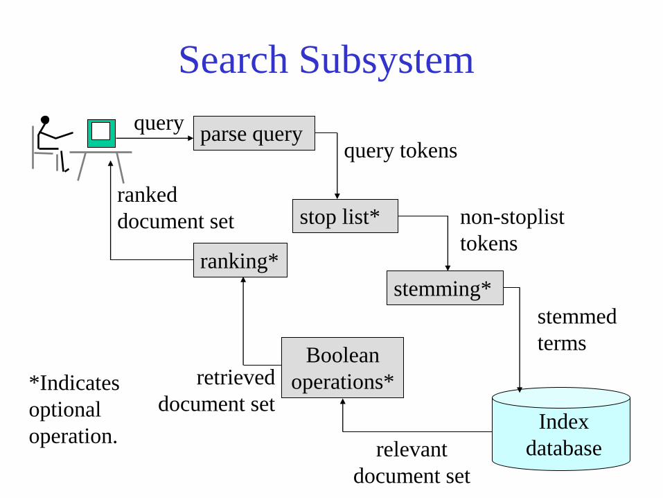
Search Subsystem

Index

database

query parse query

stemming*

stemmed

terms

stop list* non-stoplist

tokens

query tokens

Boolean

operations*

ranking*

relevant

document set

ranked

document set

retrieved

document set *Indicates

optional

operation.

Terms vs tokens

• Terms are what results after tokenization

and linguistic processing.

– Examples

• knowledge -> knowledg

• The -> the

• Removal of stop words

Matching/Ranking of Textual

Documents

Major Categories of Methods

1. Exact matching (Boolean)

2. Ranking by similarity to query (vector space model)

3. Ranking of matches by importance of documents

(PageRank)

4. Combination methods

What happens in major search engines (Googlerank)

Vector representation of documents and queries

Why do this?

• Represents a large space for documents

• Compare

– Documents

– Documents with queries

• Retrieve and rank documents with regards to a specific query

- Enables methods of similarity

All search engines do this.

Boolean queries

• Document is relevant to a query of the query itself is in the document.

– Query blue and red brings back all documents with blue and red in them

• Document is either relevant or not relevant to the query.

• What about relevance ranking – partial relevance. Vector model deals with this.

Similarity Measures and Relevance

• Retrieve the most similar documents to a

query

• Equate similarity to relevance

– Most similar are the most relevant

• This measure is one of “text similarity”

– The matching of text or words

Similarity Ranking Methods

Query Documents Index

database

Mechanism for determining the similarity

of the query to the document.

Set of documents

ranked by how similar

they are to the query

Term Similarity: Example

Problem: Given two text documents, how similar are they?

[Methods that measure similarity do not assume exact

matches.]

Example (assume tokens converted to terms)

Here are three documents. How similar are they?

d1 ant ant bee

d2 dog bee dog hog dog ant dog

d3 cat gnu dog eel fox

Documents can be any length from one word to thousands.

A query is a special type of document.

Bag of words view of a doc

Tokens are extracted from text and thrown into a “bag” without order and labeled by document.

• Thus the doc

– John is quicker than Mary.

is indistinguishable from the doc

– Mary is quicker than John.

is

John

quicker

Mary

than

Two documents are similar if they contain some of the same

terms.

Possible measures of similarity might take into consideration:

(a) The lengths of the documents

(b) The number of terms in common

(c) Whether the terms are common or unusual

(d) How many times each term appears

Term Similarity: Basic Concept

TERM VECTOR SPACE Term vector space

n-dimensional space, where n is the number of different

terms/tokens used to index a set of documents.

Vector

Document i, di, represented by a vector. Its magnitude in

dimension j is wij, where:

wij > 0 if term j occurs in document i

wij = 0 otherwise

wij is the weight of term j in document i.

A Document Represented in a

3-Dimensional Term Vector Space

t1

t2

t3

d1

t13

t12 t11

Basic Method: Incidence Matrix

(Binary Weighting)

document text terms

d1 ant ant bee ant bee

d2 dog bee dog hog dog ant dog ant bee dog hog

d3 cat gnu dog eel fox cat dog eel fox gnu

ant bee cat dog eel fox gnu hog

d1 1 1

d2 1 1 1 1

d3 1 1 1 1 1

Weights: tij = 1 if document i contains term j and zero otherwise

3 vectors in

8-dimensional

term vector

space

Basic Vector Space Methods: Similarity

between 2 documents

The similarity between

two documents is a

function of the angle

between their vectors in

the term vector space.

t1

t2

t3

d1 d2

Vector Space Revision x = (x1, x2, x3, ..., xn) is a vector in an n-dimensional vector space

Length of x is given by (extension of Pythagoras's theorem)

|x|2 = x12 + x2

2 + x32 + ... + xn

2

|x| = ( x12 + x2

2 + x32 + ... + xn

2 )1/2

If x1 and x2 are vectors:

Inner product (or dot product) is given by

x1.x2 = x11x21 + x12x22 + x13x23 + ... + x1nx2n

Cosine of the angle between the vectors x1 and x2:

cos () = x1.x2

|x1| |x2|

Document similarity d = (x1, x2, x3, ..., xn) is a vector in an n-dimensional vector space

Length of x is given by (extension of Pythagoras's theorem)

|d|2 = x12 + x2

2 + x32 + ... + xn

2

|d| = ( x12 + x2

2 + x32 + ... + xn

2 )1/2

If d1 and d2 are document vectors:

Inner product (or dot product) is given by

d1.d2 = x11x21 + x12x22 + x13x23 + ... + x1nx2n

Cosine angle between the docs d1 and d2 determines doc similarity

cos () = d1.d2

|d1| |d2|

cos () = 1; documents exactly the same; = 0, totally different

Example 1

No Weighting

ant bee cat dog eel fox gnu hog length

d1 1 1 2

d2 1 1 1 1 4

d3 1 1 1 1 1 5

Ex: length d1 = (12+12)1/2

Example 1 (continued)

d1 d2 d3

d1 1 0.71 0

d2 0.71 1 0.22

d3 0 0.22 1

Similarity of documents in example:

Digression: terminology

• WARNING: In a lot of IR literature, “frequency” is used to mean “count”

– Thus term frequency in IR literature is used to mean number of occurrences in a doc

– Not divided by document length (which would actually make it a frequency)

• We will conform to this misnomer

– In saying term frequency we mean the number of occurrences of a term in a document.

Example 2

Weighting by Term Frequency (tf)


d1 2 1 5

d2 1 1 4 1 19

d3 1 1 1 1 1 5

Weights: tij = frequency that term j occurs in document i

document text terms




Example 2 (continued)

d1 d2 d3

d1 1 0.31 0

d2 0.31 1 0.41

d3 0 0.41 1

Similarity of documents in example:

Similarity depends upon the weights given to the terms.

[Note differences in results from Example 1.]

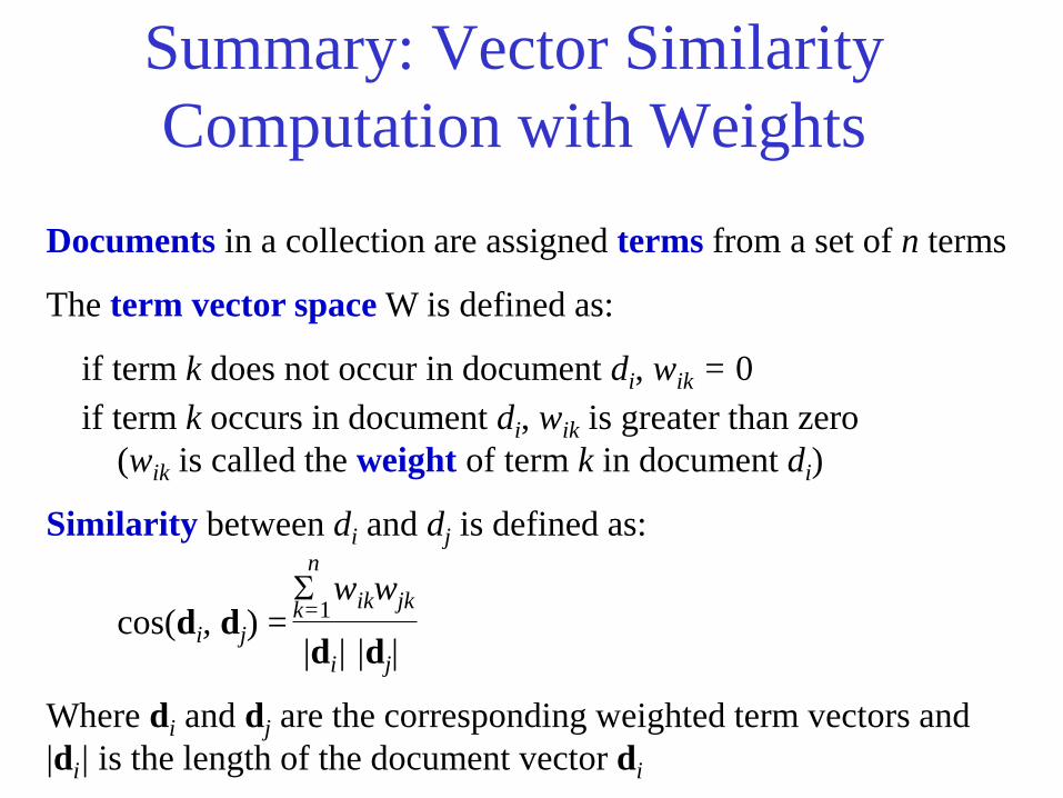
Summary: Vector Similarity

Computation with Weights

Documents in a collection are assigned terms from a set of n terms

The term vector space W is defined as:

if term k does not occur in document di, wik = 0

if term k occurs in document di, wik is greater than zero

(wik is called the weight of term k in document di)

Similarity between di and dj is defined as:

wikwjk

|di| |dj|

Where di and dj are the corresponding weighted term vectors and

|di| is the length of the document vector di

k=1

n

cos(di, dj) =

Summary: Vector Similarity

Computation with Weights

Inner product (or dot product) between documents

d1.d2 = w11w21 + w12w22 + w13w23 + ... + w1nw2n

Inner product (or dot product) is between a document and query

d1.q1 = w11wq11 + w12wq12 + w13wq13 + ... + w1nwq1n

where wqij is the weight of the jth term of the ith query

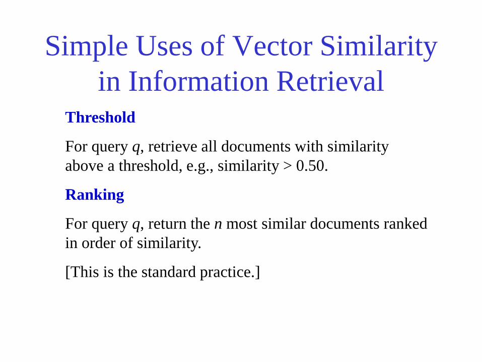
Simple Uses of Vector Similarity

in Information Retrieval Threshold

For query q, retrieve all documents with similarity

above a threshold, e.g., similarity > 0.50.

Ranking

For query q, return the n most similar documents ranked

in order of similarity.

[This is the standard practice.]

Simple Example of Ranking

(Weighting by Term Frequency)


q 1 1 √2

d1 2 1 5

d2 1 1 4 1 19

d3 1 1 1 1 1 5

query

q ant dog

document text terms




Calculate Ranking

d1 d2 d3

q 2/√10 5/√38 1/√10

0.63 0.81 0.32

Similarity of query to documents in example:

If the query q is searched against this

document set, the ranked results are:

d2, d1, d3

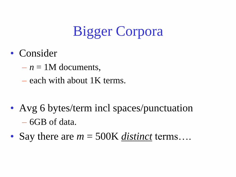
Bigger Corpora

• Consider

– n = 1M documents,

– each with about 1K terms.

• Avg 6 bytes/term incl spaces/punctuation

– 6GB of data.

• Say there are m = 500K distinct terms….

Can’t Build the Matrix

• 500K x 1M matrix: 500 Billion 0’s and 1’s.

• But it has no more than 1 billion 1’s.

– matrix is extremely sparse.

• What’s a better representation?

Documents are parsed to extract

words and these are saved with the

document ID.

I did enact Julius

Caesar I was

killed i' the

Capitol; Brutus

killed me.

Doc 1

So let it be with

Caesar. The

Noble Brutus hath

told you Caesar

was ambitious

Doc 2

Term Doc #

I 1

did 1

enact 1

julius 1

caesar 1

I 1

was 1

killed 1

i' 1

the 1

capitol 1

brutus 1

killed 1

me 1

so 2

let 2

it 2

be 2

with 2

caesar 2

the 2

noble 2

brutus 2

hath 2

told 2

you 2

caesar 2

was 2

ambitious2

Inverted index

Later, sort inverted file by terms

Term Doc #

ambitious 2

be 2

brutus 1

brutus 2

capitol 1

caesar 1

caesar 2

caesar 2

did 1

enact 1

hath 1

I 1

I 1

i' 1

it 2

julius 1

killed 1

killed 1

let 2

me 1

noble 2

so 2

the 1

the 2

told 2

you 2

was 1

was 2

Term Doc #

I 1

did 1

enact 1

julius 1

caesar 1

I 1

was 1

killed 1

i' 1

the 1

capitol 1

brutus 1

killed 1

me 1

so 2

let 2

it 2

be 2

with 2

caesar 2

the 2

noble 2

brutus 2

hath 2

told 2

you 2

caesar 2

was 2

ambitious 2

• Multiple term

entries in a single

document are

merged and

frequency

information added

Term Doc # Freq

ambitious 2 1

be 2 1

brutus 1 1

brutus 2 1

capitol 1 1

caesar 1 1

caesar 2 2

did 1 1

enact 1 1

hath 2 1

I 1 2

i' 1 1

it 2 1

julius 1 1

killed 1 2

let 2 1

me 1 1

noble 2 1

so 2 1

the 1 1

the 2 1

told 2 1

you 2 1

was 1 1

was 2 1

with 2 1

Term Doc #

ambitious 2

be 2

brutus 1

brutus 2

capitol 1

caesar 1

caesar 2

caesar 2

did 1

enact 1

hath 1

I 1

I 1

i' 1

it 2

julius 1

killed 1

killed 1

let 2

me 1

noble 2

so 2

the 1

the 2

told 2

you 2

was 1

was 2

with 2

Best Choice of Weights?

ant bee cat dog eel fox gnu hog

q ? ?

d1 ? ?

d2 ? ? ? ?

d3 ? ? ? ? ?

query

q ant dog

document text terms




What

weights lead

to the best

information

retrieval?

Weighting

Term Frequency (tf) Suppose term j appears fij times in document i. What

weighting should be given to a term j?

Term Frequency: Concept

A term that appears many times within a document is

likely to be more important than a term that appears

only once.

Term Frequency: Free-text

Document

Length of document

Simple method is to use wij as the term frequency.

...but, in free-text documents, terms are likely to

appear more often in long documents. Therefore wij

should be scaled by some variable related to document

length.

i

Term Frequency: Free-text Document A standard method for free-text documents

Scale fij relative to the frequency of other terms in the

document. This partially corrects for variations in the

length of the documents.

Let mi = max (fij) i.e., mi is the maximum frequency of

any term in document i.

Term frequency (tf):

tfij = fij / mi when fij > 0

Note: There is no special justification for taking this

form of term frequency except that it works well in

practice and is easy to calculate.

i

Weighting

Inverse Document Frequency (idf) Suppose term j appears fij times in document i. What

weighting should be given to a term j?

Inverse Document Frequency: Concept

A term that occurs in a few documents is likely to be a

better discriminator than a term that appears in most or

all documents.

Inverse Document Frequency Suppose there are n documents and that the number of

documents in which term j occurs is nj.

A possible method might be to use n/nj as the inverse

document frequency.

A standard method

The simple method over-emphasizes small differences.

Therefore use a logarithm.

Inverse document frequency (idf):

idfj = log2 (n/nj) + 1 nj > 0

Note: There is no special justification for taking this form

of inverse document frequency except that it works well in

practice and is easy to calculate.

Example of Inverse Document

Frequency Example

n = 1,000 documents; nj # of docs term appears in

term j nj idfj

A 100 4.32

B 500 2.00

C 900 1.13

D 1,000 1.00

From: Salton and McGill idfj modifies only the columns not

the rows!

Full Weighting:

A Standard Form of tf.idf

Practical experience has demonstrated that weights of the following

form perform well in a wide variety of circumstances:

(weight of term j in document i)

= (term frequency) * (inverse document frequency)

A standard tf.idf weighting scheme, for free text documents, is:

tij = tfij * idfj

= (fij / mi) * (log2 (n/nj) + 1) when nj > 0

Discussion of Similarity

The choice of similarity measure is widely used and works

well on a wide range of documents, but has no theoretical

basis.

1. There are several possible measures other that angle

between vectors

2. There is a choice of possible definitions of tf and idf

3. With fielded searching, there are various ways to adjust the

weight given to each field.

Similarity Measures Compared

|)||,min(|

||

||||

||

||

||

||||

||2

||

21

21

DQ

DQ

DQ

DQ

DQ

DQ

DQ

DQ

DQ

Simple matching (coordination level match)

Dice’s Coefficient

Jaccard’s Coefficient

Cosine Coefficient (what we studied)

Overlap Coefficient

Similarity Measures

• A similarity measure is a function which computes the degree of

similarity between a pair of vectors or documents

– since queries and documents are both vectors, a similarity measure

can represent the similarity between two documents, two queries, or

one document and one query

• There are a large number of similarity measures proposed in the

literature, because the best similarity measure doesn't exist (yet!)

• With similarity measure between query and documents

– it is possible to rank the retrieved documents in the order of

presumed importance

– it is possible to enforce certain threshold so that the size of the

retrieved set can be controlled

– the results can be used to reformulate the original query in

relevance feedback (e.g., combining a document vector with the

query vector)

Problems

• Synonyms: separate words that have the same meaning. – E.g. ‘car’ & ‘automobile’

– They tend to reduce recall

• Polysems: words with multiple meanings – E.g. ‘Java’

– They tend to reduce precision

The problem is more general: there is a disconnect between topics and words

• ‘… a more appropriate model should consider some

conceptual dimensions instead of words.’

(Gardenfors)

Latent Semantic Analysis (LSA)

• LSA aims to discover something about the meaning

behind the words; about the topics in the documents.

• What is the difference between topics and words?

– Words are observable

– Topics are not. They are latent.

• How to find out topics from the words in an automatic

way?

– We can imagine them as a compression of words

– A combination of words

– Try to formalise this

Latent Semantic Analysis • Singular Value Decomposition (SVD)

A(m*n) = U(m*r) E(r*r) V(r*n)

Keep only k eigen values from E

A(m*n) = U(m*k) E(k*k) V(k*n)

Convert terms and documents to points in k-dimensional space

• Singular Value Decomposition

{A}={U}{S}{V}T

• Dimension Reduction

{~A}~={~U}{~S}{~V}T

Latent Semantic Analysis

Latent Semantic Analysis

• LSA puts documents together even if they

don’t have common words if

– The docs share frequently co-occurring terms

• Disadvantages:

– Statistical foundation is missing

PLSA addresses this concern!

PLSA

• Generative Model

– Select a doc with probability P(d)

– Pick a latent class z with probability P(z|d)

– Generate a word w with probability p(w|z)

d z w P(d) P(z|d) P(w|z)

Latent Variable model for general co-occurrence data

Associate each observation (w,d) with a class variable z Є

Z{z_1,…,z_K}

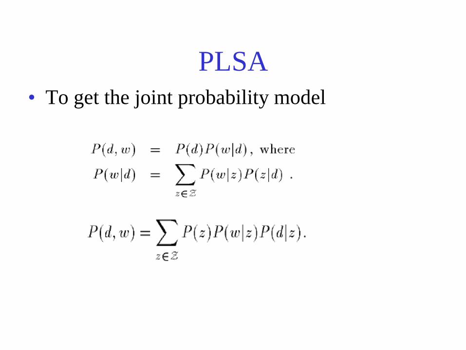
PLSA

• To get the joint probability model

Model fitting with EM

• We have the equation for log-likelihood

function from the aspect model, and we

need to maximize it.

• Expectation Maximization ( EM) is used for

this purpose

EM Steps

• E-Step

– Expectation step where expectation of the

likelihood function is calculated with the

current parameter values

• M-Step

– Update the parameters with the calculated

posterior probabilities

– Find the parameters that maximizes the

likelihood function

E Step

• It is the probability that a word w occurring

in a document d, is explained by aspect z

(based on some calculations)

M Step

• All these equations use p(z|d,w) calculated in E

Step

• Converges to local maximum of the likelihood

function

The performance of a retrieval system based on this model (PLSI)

was found superior to that of both the vector space based similarity

(cos) and a non-probabilistic latent semantic indexing (LSI) method.

(We skip details here.)

From Th. Hofmann, 2000

Comparing PLSA and LSA

• LSA and PLSA perform dimensionality reduction – In LSA, by keeping only K singular values

– In PLSA, by having K aspects

• Comparison to SVD – U Matrix related to P(d|z) (doc to aspect)

– V Matrix related to P(z|w) (aspect to term)

– E Matrix related to P(z) (aspect strength)

• The main difference is the way the approximation is done – PLSA generates a model (aspect model) and maximizes its

predictive power

– Selecting the proper value of K is heuristic in LSA

– Model selection in statistics can determine optimal K in PLSA