KNEE JOINT LOADING IN THE OPEN AND SQUARE

STANCE TENNIS FOREHANDS

Paul Sandamas

Paul Sandamas

Spring 2013

Department of Biology of Physical Activity

University of Jyväskylä

Supervisor: Professor J. Avela

ABSTRACT

Sandamas, Paul 2013. Knee joint loading in the open and square stance tennis

forehands. Department of Biology of Physical Activity, University of Jyväskylä.

Master's Thesis in Biomechanics. 80 pages.

The aim of this study was to calculate and compare the resultant forces and moments in

the knee joint of the open and square stance tennis forehands. An additional aim was to

incorporate the ground reaction forces to shed light on the role of the lower body in

aiding pelvic rotation in these two different forehands.

The two types of forehand strokes hit by 7 right-handed university team level tennis

players were filmed and the ground reaction forces on each foot were measured

simultaneously. A link segment model of the lower limbs was used along with the

inverse dynamics approach to calculate the resultant joint forces and moments in both

knees during both the forward swing and follow-through phases of the shot. The

ground reaction forces and resultant knee joint forces and moments of the open stance

(OS) strokes were compared with those obtained for the square stance (SS) forehands.

Although the average swing times, peak racket velocities and peak transverse plane

pelvic velocities were similar, significant kinetic differences (P<0.05) were recorded in

the knee joints between the strokes. The SS created greater abduction moments in the

left knee during the forward swing and follow-through (0.7 and 0.95 Nm/kg) than the

OS (0.2 and 0.32 Nm/kg), respectively. The largest external rotation moments were

found in the SS left knee during the follow-through (0.31 Nm/kg) and in the OS right

knee prior to impact (0.24 Nm/kg). Despite this, significantly (P<0.05) greater ground

reaction torque (TZ) was generated by the right leg in the OS stroke before impact (0.27

Nm/kg), than by the left leg in the SS during the follow-through (0.09 Nm/kg).

The data did not support the hypothesis that the peak knee external rotation moments

would be greater in the square stance. Analysis of the ground reaction forces together

with the knee kinetic and pelvic motion data suggests that the square stance utilises the

forward step as an aid to pelvic rotation, whereas; the open stance relies more on the

extension, abduction and external rotation of the right leg to aid pelvic rotation.

Keywords: tennis forehand, inverse dynamics, knee joint loading, free moment.

ABBREVIATIONS AND DEFINITIONS

OS = Open stance

SS = Square stance

CS = Closed stance

GRF = Ground reaction force

GRFV = Ground reaction force vector

Fz = Vertical component of the GRF

Tz = Vertical torque (free moment)

CoP = Centre of pressure

CoM = Centre of mass

JCS = Joint coordinate system

LCS = Local coordinate system

GCS = Global coordinate system

ASIS = Anterior superior iliac spine

Prox = Proximal

Dist = Distal

Med = Medial

Lat = Lateral

Ant = Anterior

Pos = Posterior

Flex = Flexion

Ext = Extension

Abd = Abduction

Add = Adduction

Int Rot = Internal rotation

Ext Rot = External rotation

In the literature, the terms moment and torque are often used interchangeably. In this

study, the term moment is used when referring to the resultant joint moment, whereas

the term torque is used to describe the moment applied to the foot about the vertical axis

from a force plate.

A vector is donated in boldface type and scalars are printed in italic. The axes denoting

the global coordinate system are in capitals whereas the axes of the local coordinate

system are in lower case.

The following descriptions of tennis technique all refer to right-handed players.

TABLE OF CONTENTS

ABSTRACT ………………………………………………………………….………....1

1 INTRODUCTION ……………………………………………….…………………...6

2 BIOMECHANICS OF THE TENNIS FOREHAND ……….………………………..7

2.1 Preparation ……………………………….……………………………………. 7

2.1.1 The open stance forehand……………………………………...….......8

2.1.2 The square stance forehand ………….…………………..………..….8

2.1.3 Ground reaction forces in the forehand…..….……………………..…9

2.1.4 Differences between the open stance and square stance forehands….10

2.2 Backswing ……………………………………………………………………11

2.3 Forward stroke ……………………………………………………………….12

2.3.1 The role of the lower body in rotating the pelvis ….……………….13

2.4 Follow-through ……………………………………………………………….14

3 THREE DIMENSIONAL JOINT KINETICS ……………………………………...15

3.1 Inverse dynamics …………………………………………………………..…15

3.1.1 Free body diagram………………...………...………...…………..…16

3.1.2 Ground reaction forces …………………………...………….…..….17

3.1.3 Equations of motion: forces …………………….………..……….…18

3.1.4 Equations of motion: moments ……………………………….…..…20

3.1.5 Equations of motion: angular kinematics ………...………....………24

3.1.6 Limitations of the inverse dynamics model ………...……….…...….25

3.2 Estimating muscle activity with the ground reaction force vector ...…………26

4 PURPOSE OF THE STUDY ………….………………………...………………….28

5 METHOD ……………………………………………………………….…………..29

5.1 Subjects ……………………………………………………………………….29

5.2 Experimental procedure ………………………………………………………29

5.3 Analytical procedures ……………………………..………………………….32

5.4 Expression of joint forces and moments.……………………..………………38

5.5 Statistical methods ……………………………………………….….………..38

6 RESULTS …………………………………………………………..…………….…40

6.1 Stroke parameters ………………………………………………………….…40

6.2 Ground reaction forces ……………………………………………………….40

6.2.1 Weight transfer ….…………..……………………………………40

6.2.2 Vertical torque ……………………………………………………41

6.2.3 Medial/lateral and anterior/posterior ground reaction forces …….42

6.3 Body movements based on marker data ………………………………….…..43

6.3.1 Comparison of pelvic motion ……………...……………………..43

6.3.2 Knee angles ……………………………………………………….45

6.3.3 Peak knee external rotation moment versus knee flexion angle ….45

6.4 Forces and moments of the knee joint …………………………………..……46

6.4.1 Open stance …………………………………………….…………46

6.4.2 Square stance ……………………………………………..………48

6.4.3 Internal/external rotation moments ..........................................…...50

6.4.4 Kinetic comparison of the open and square stance strokes …….…51

7 DISCUSSION ……………………………………………………………………….52

7.1 Stroke parameters ……………………………………………………...……..52

7.2 Comparison with the literature …………………………………….…………53

7.3 Open stance forces and moments …………………………………….………55

7.4 Square stance forces and moments …………………………………………...58

7.5 Suggestion for the role of the lower extremities in generating pelvic

rotation…………………………………………………………………..……61

7.6 Error sources and limitations ……………………………...….………………62

7.7 Coaching implications …………………………………………………..……63

7.8 Suggestions for further study ……………..………………………..…………63

8 CONCLUSIONS ………………………………………………………...………….65

9 REFERENCES …..………………………………………………….………………66

10 APPENDIX ………………………………………………………………..………72

10.1 Definition of the Euler angles using the Z, line of nodes, z rotation …….…72

sequence

10.2 Angular velocity of the segment ………..………………………………….74

10.3 Angular acceleration of the segment ……………………………………..…76

10.4 Examples of selected raw data .…..……………….…………………...……77

1 INTRODUCTION

Tennis is a popular sport played throughout the world. It is estimated about 75 million

people play tennis regularly (Pluim et al. 2007). Despite this there is very little

published data concerning three dimensional tennis biomechanics and almost nothing

related to lower limb kinetics of the forehand.

After the serve, the forehand is the most important shot in a player’s arsenal. Rotation

of both the upper body and lower body has been described as a significant source of

power in the forehand stroke (Groppel 1992, 41; Bollettieri 2001, 118; Elliott 2002, 11;

Knudson 2006, 75). The energy is transferred upward from the legs to the pelvis,

through the trunk to the arm and then to the racket (Perry et al. 2004). In the kinetic

chain of the lower body, the knee joint is regarded as the “critical middle link” in the

proximal transfer of force (Whiting & Zernicke 1998, 157). The rotation of the pelvis

and trunk involves torsional forces in the lower body, not only during the forward swing

but also during the follow-through in which this rotational energy is being dissipated.

Research on the lower limb kinetics of the closed stance (CS) forehand has shown that a

leg drive was essential to create high axial hip rotational torques to aid trunk rotation

(Iino & Kojima 2001; 2003). Only sagittal plane knee moments were described in these

studies.

However, most forehands are now hit with an open stance (OS) (Roetert et al. 2009).

To date, no data on the lower body kinetics or ground reaction forces of the OS

forehand or square stance (SS) forehands have been published. Also, no data

concerning the lower body forces found during the follow-through phase of neither the

OS nor the SS forehand have been published. Therefore, the main aim of this study is

to calculate and compare the forces and moments in the knee joint in both the OS and

SS forehand during both the forward swing and follow-through phases. The secondary

aim is to incorporate the ground reaction force data to gain information about the role of

the lower body in rotating the pelvis in the OS and SS forehands.

7

2 BIOMECHANICS OF THE TENNIS FOREHAND

The following is a description of the biomechanics of the tennis forehand that is most

relevant to this study. This description is based on four major temporal phases of the

stroke: preparation, backswing, swing to impact and follow-through.

2.1 Preparation

The two biomechanical issues relating to the preparation for a tennis stroke are

readiness and stance.

Readiness. A good ready position or “split step” is important as it enables the player to

move quickly to intercept the opponent’s shot (Groppel 1992, 41). A split step involves

timing a small hop that coincides with the opponent striking the ball. This hop involves

knee flexion followed by extension. By using a split step the player benefits from the

stretch-shortening cycle (Komi & Nicol 2000, 87) which has been quoted as enhancing

the speed of movement by approximately 15-20% (Knudson & Elliott 2004, 154).

Stance. As much of the force used to hit the ball is transferred up through the body to

the racket arm (Groppel 1992, 79), the way the player positions their feet will effect

how this force is generated and transferred. Stances fall on a continuum between open

and closed (Knudson 2006, 81). The positions of the feet for the three main stances are

illustrated in figure 2.1.

8

A

B C

Target line

FIGURE 2.1. Position of the feet for the three main type of stance. Open stance (A), square

stance (B) and closed stance (C). The right foot is in the same position for the three stances

depicted. Modified from Knudson (2006, 82).

2.1.1 The open stance forehand

To execute an open stance (OS) forehand, the player faces the court with their pelvis

roughly parallel to the net (hence the name “open”) and rotates the shoulders away from

the court during the backswing and towards the court during the forward swing (Crespo

& Reid 2003, 24). The OS forehand is likely to utilise both linear and angular

momentum, although the amount of linear momentum is likely to be less than in the

square stance (SS) forehand (Knudson 2006, 84). An example of an OS forehand is

shown in figure 2.1 (a). This is the type of forehand that is used the most in tennis

(Roetert et al. 2009).

2.1.2 The square stance forehand

The square stance (SS) forehand has been described as the “traditional” forehand as

opposed to the “modern” or OS forehand (Crespo & Higueras 2001, 149). To execute a

SS forehand, the player pivots on the rear leg and takes a step toward the ball thereby

placing their pelvis and feet perpendicular to the intended direction of the shot (hence

the name “square”). This stepping action transfers their weight from the rear foot onto

9

the leading foot just prior to contact with the ball (Bahamonde & Knudson 2003). An

example of the SS forehand is shown in figure 2.2.

FIGURE 2.2. The SS forehand. Notice that the weight has been transferred to the leading leg

before contact in the SS forehand

According to Groppel (1992, 10) and Knudson (2006, 84), the weight transfer has been

highlighted as an important source of power in this type of stroke because the forward

step generates an amount of linear momentum that is converted into angular momentum

during the forward swing.

2.1.3 Ground reaction forces in the forehand

Published data from the closed and SS forehands has shown that the weight transfer

occurs before impact and that the body first accelerates and then decelerates prior to

impact. An example of the weight transfer and forward and braking impulses occurring

before impact in the sideways on type forehands is shown in figure 2.3.

10

Fo

rce

(B

W)

Time (s)

-0.8 -0.6 -0.4 -0.2 0

Left

Right0

0

.5

1

Fo

rce (

N)

Time

Propulsive impulse

Braking impulse

-100

0

100

Impact

a) b)

FIGURE 2.3. a) The vertical ground reaction forces showing the transfer of weight from the

right leg to the left before impact during the closed stance forehand. Ball impact occurs at time

= 0 seconds. Adapted from Iino and Kojima (2001). b) Anterior/posterior force plate graph that

shows the body first accelerates and then decelerates just prior to impact. Adapted from Van

Gheluwe and Hebbelinck (1986).

No ground reaction torque values have been published for tennis shots, although they

have been used to study the kinetics at the shoe-surface interface in golf. In golf the

term range has been used to quantify the change in direction of the ground reaction

torque. Range of the torque was defined as from peak clockwise TZ to peak counter-

clockwise TZ torque (Worsfold et al. 2008).

2.1.4 Differences between the open stance and square stance forehands

A comparison of the main features of the OS and SS forehand strokes is given in table

2.1. Although the position of the feet is different between the strokes, the motions of

the trunk, arm and racket have been shown to be similar (Crespo & Higueras 2001,

150).

11

TABLE 2.1. Comparison of the OS and SS forehands. (Crespo & Higueras 2001, 151; Saviano

1997.

Open stance (OS) Square stance (SS)

Preparation time Shorter Longer

Initial footwork Slight step to the sideline Step forward

Hip position Facing the net Facing the sideline

Optimal hitting zone Between shoulder and

waist height

Between knee and waist

height

Amount of pelvic rotation More Less

Recovery time Shorter Longer

Since modern tennis is played at a high speed on hard surfaces that give a higher

bouncing ball (Saviano 1997), the OS is the shot of choice for three main reasons: a)

less preparation and recovery time is required, b) it enables powerful shots to be hit off

high bouncing balls and c) modern light-weight rackets allow for powerful strokes even

with an abbreviated backswing.

There have been concerns about the injury risk of the modern OS forehands compared

to the traditional forehand. Trunk muscle activity (Knudson & Blackwell 2000) and the

loads in the racket arm (Bahamonde & Knudson 2003) have been studied with the

conclusion that that there was no significant injury risk of the OS compared to the SS.

2.2 Backswing

The backswing is essential for power generation. In the backswing phase the player

typically flexes the knees while the shoulders rotate backwards more than the pelvis

creating “a coiling effect” which pre-stretches the muscles of the chest/shoulder and

trunk (Elliott 2003, 35). The difference between the alignment of the upper part of the

trunk and the pelvis is known as the “separation angle” (figure 2.4). The pre-stretching

of the muscles around the pelvis during the backswing is sometimes called “hip

loading” in coaching texts (Bollettieri 2001, 114).

12

The backswing also helps to generate power by increasing the distance and time over

which the speed of the racket can be increased during the forward stroke (Elliott 2003,

33).

θ

FIGURE 2.4. Separation angle. The angle between the alignment of the shoulders and the

pelvis (Elliott 2003, 35).

2.3 Forward stroke

The purpose of the forward stroke is to generate racket head speed and accurate racket

movement to intercept the ball. The racket head speed at impact is the major

contributor to the ball speed of the shot (Elliot et al. 1997). The biomechanical issues

are recovery of the elastic energy in the stretch-shortening cycle and coordination of the

body segments necessary to hit the ball.

In the forward swing the energy stored in the muscle tendon unit during the backswing

is converted to the kinetic energy of the segment. In addition, the initial rotation of the

trunk creates a stretch of the shoulder muscles which enhances its ability to create a

forceful forward swing of the arm (Elliott 2003, 35).

The coordinated activation of the body segments in order to hit the ball is commonly

referred to in coaching as the kinetic chain (Kibler & van der Meer 2001, 100). The

chain consists of the lower body, pelvis, trunk, arm, hand and finally the racket. The

13

goal of a kinetic chain is to place the racket in the optimum position at the optimum

velocity to strike the ball. By using the kinetic chain, the player can transfer the large

forces created by the ground reaction forces up through the body to the racket (Perry et

al. 2004; Knudson 2006, 8). In the forehand, the hips, trunk, shoulder, elbow, wrist and

the racket have been shown to reach peak velocity in sequence (Landlinger et al. 2010).

This type of sequential coordination conforms to the “summation of speed principle”

(Marshall & Elliott, 2000). The one notable exception in the proximal-to-distal

sequencing of the arm segments is internal rotation of the upper arm which reaches its

peak angular velocity just before (Elliott 2002, 5) or even just after impact (Landlinger

et al. 2010).

2.3.1 The role of the lower body in rotating the pelvis.

Research on the closed stance (CS) forehand has highlighted the roles of the hips in

rotating the pelvis. The right hip abduction and external rotation moments plus right hip

and knee extension moments all contribute to the generation of pelvic torque in the

transverse plane (Iino & Kojima 2001; 2003). The reason these hip moments contribute

to pelvic torque can be explained by viewing the projections of these vectors onto the

superior/inferior axis of the pelvis (figure 2.5).

a) b)

FIGURE 2.5. The effect of the attitude of the right hip joint on the contributions of a) the hip

extension moment and b) the abduction moment to the pelvic torque (Iino and Kojima 2001).

Thus for the right hip to rotate the pelvis using extension and abduction moments, the

hip must be in a flexed and abducted position. The abducted position aids the role of

14

the hip extension moment to rotate the pelvis (figure 2.5a) while hip flexion aids the

role of the hip abduction moment to rotate the pelvis (figure 2.5b). The projection of

the right hip external rotation vector will be parallel to the pelvis superior/inferior axis

when the lower body is in the anatomical position. This means that the external rotation

moment of the hip can contribute the most when the thigh is neither flexed nor abducted

(Iino & Kojima 2001).

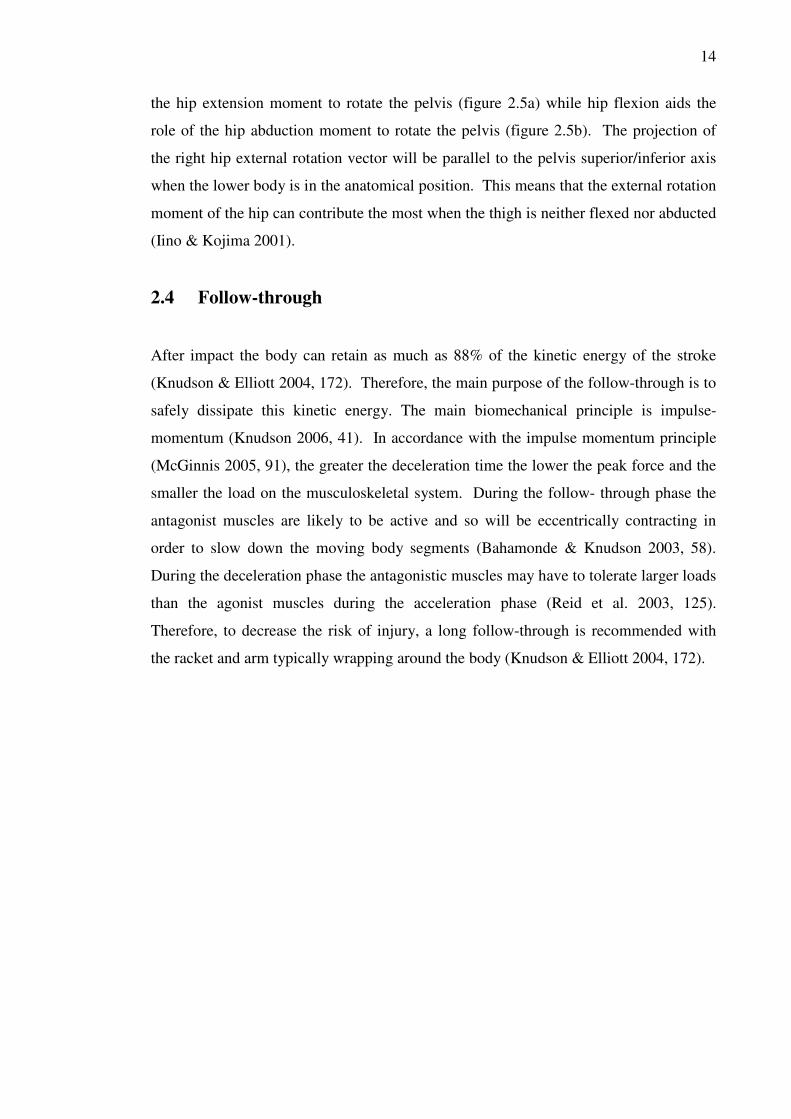
2.4 Follow-through

After impact the body can retain as much as 88% of the kinetic energy of the stroke

(Knudson & Elliott 2004, 172). Therefore, the main purpose of the follow-through is to

safely dissipate this kinetic energy. The main biomechanical principle is impulse-

momentum (Knudson 2006, 41). In accordance with the impulse momentum principle

(McGinnis 2005, 91), the greater the deceleration time the lower the peak force and the

smaller the load on the musculoskeletal system. During the follow- through phase the

antagonist muscles are likely to be active and so will be eccentrically contracting in

order to slow down the moving body segments (Bahamonde & Knudson 2003, 58).

During the deceleration phase the antagonistic muscles may have to tolerate larger loads

than the agonist muscles during the acceleration phase (Reid et al. 2003, 125).

Therefore, to decrease the risk of injury, a long follow-through is recommended with

the racket and arm typically wrapping around the body (Knudson & Elliott 2004, 172).

15

3 THREE DIMENSIONAL JOINT KINETICS

The direct measurement of the internal forces acting on the joint components such as

the joint surface, tendons and ligaments requires very invasive techniques (Robertson et

al. 2004, 99). Studies have been performed to directly measure tendon forces in humans

using buckle transducers (Gregory at al. 1991) and fibre-optic transducers (Komi et al.

1996; Finni et al. 1998). A more common non-invasive method is to create a model and

obtain the resultant joint reaction forces and moments using the inverse dynamics

approach.

3.1 Inverse dynamics

The inverse dynamics approach involves obtaining information about segment

kinematics, anthropometric measures and external forces and uses this data to calculate

the resultant internal joint reaction forces and moments responsible for the movement

under focus (Enoka 2008, 124). A descriptive overview of the inverse approach is

shown in figure 3.1. The key parts of the inverse dynamics approach are the free body

diagram and the equations of motion.

Anthropometry of

skeletal segments

Segment

displacements

Ground reaction

forces

Segment masses and

moments of inertia

Velocities and

accelerations

Equations of

motion

Joint forces and

moments

FIGURE 3.1. Flowchart for the inverse dynamics approach (Adapted from Vaughan et al.

(1999, 4).

16

3.1.1 Free body diagram

A free body diagram contains the segments under focus that have been separated from

their adjacent segments and all the external forces and moments acting on these

segments (Hamill & Knutzen 2003, 350). The free body diagram of the six lower body

segments is shown in figure 3.2.

Z

Y

X

FIGURE 3.2. Free body diagram for the lower body segments. The diagram shows the

resultant external forces acting on each segment. In accordance with Newton’s 3rd

law of

motion, the forces and moments at the knee and ankle joints are equal in magnitude but opposite

in direction, depending on the segment concerned. M = joint moment, F = joint force, TZ =

ground reaction torque, m = segment mass and g = acceleration due to gravity (Vaughan et al.

(1999, 102-106).

Segment masses and moments of inertia. The segment masses and moments of inertia

can be estimated by taking anthropometric measurements such as foot breadth and calf

circumference and inputting these values into specific regression equations (Winter

2004, 63; Vaughan et al 1999, 85; Zatsiorsky 2002, 575-582).

17

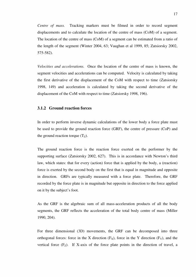
Centre of mass. Tracking markers must be filmed in order to record segment

displacements and to calculate the location of the centre of mass (CoM) of a segment.

The location of the centre of mass (CoM) of a segment can be estimated from a ratio of

the length of the segment (Winter 2004, 63; Vaughan et al 1999, 85; Zatsiorsky 2002,

575-582).

Velocities and accelerations. Once the location of the centre of mass is known, the

segment velocities and accelerations can be computed. Velocity is calculated by taking

the first derivative of the displacement of the CoM with respect to time (Zatsiorsky

1998, 149) and acceleration is calculated by taking the second derivative of the

displacement of the CoM with respect to time (Zatsiorsky 1998, 196).

3.1.2 Ground reaction forces

In order to perform inverse dynamic calculations of the lower body a force plate must

be used to provide the ground reaction force (GRF), the centre of pressure (CoP) and

the ground reaction torque (TZ).

The ground reaction force is the reaction force exerted on the performer by the

supporting surface (Zatsiorsky 2002, 627). This is in accordance with Newton’s third

law, which states: that for every (action) force that is applied by the body, a (reaction)

force is exerted by the second body on the first that is equal in magnitude and opposite

in direction. GRFs are typically measured with a force plate. Therefore, the GRF

recorded by the force plate is in magnitude but opposite in direction to the force applied

on it by the subject’s foot.

As the GRF is the algebraic sum of all mass-acceleration products of all the body

segments, the GRF reflects the acceleration of the total body centre of mass (Miller

1990, 204).

For three dimensional (3D) movements, the GRF can be decomposed into three

orthogonal forces: force in the X direction (FX), force in the Y direction (FY), and the

vertical force (FZ). If X-axis of the force plate points in the direction of travel, a

18

positive FX will be a propulsive force while a negative FX will be a braking force.

Examples of propulsive and braking forces are shown in figure 2.3b. The same

principle applies to motion in the Y direction.

In addition, the location of the resultant GRF in the X, Y plane is required. This is

known as the centre of pressure (Zatsiorsky 2002, 46). The location of the CoP is

critically important for calculating flexion/extension and abduction/adduction joint

moments as it determines the length of the moment arm used in calculating the

moments acting on the ankle (Winter 2005, 102).

The final value that the force plate must provide is the ground reaction torque, which is

the torque applied to the foot about the vertical Z axis (Vaughan et al. 1999, 36). This

torque acts on a plane parallel to the surface of the force plate (figure 3.3) and is

sometimes called the free moment (Miller 1990, 220). The ground reaction torque is

especially important for calculating internal/external rotation moments of the lower

body during movements that involve twisting (Grimshaw et al. 2006, 332). The

location of (TZ) is the coordinates of the centre of pressure.

Tz

CoP

FIGURE 3.3. Depiction of the ground reaction torque when looking down onto the force plate

(Grimshaw et al. 2006, 332).

3.1.3 Equations of motion: Forces

A variety of methods can be used to obtain the equations of motion in dynamic

musculoskeletal modelling, such as Lagrange (Andrews 1995, 154), the Kane method

(Yamaguchi 2004, 173) and Newton-Euler (Vaughan et al. 1992, 83). The advantage of

the Newton-Euler equations is that they enable the joint reaction forces to be calculated.

19

In the Newton-Euler approach, the joint reaction forces are calculated by applying the

linear form of Newton’s second law, and the joint moments are calculated by applying

Euler’s equations of motion to the angular form of Newton’s second law (Siegler & Liu

1997). The joint reaction forces are calculated first and are then used as inputs to

calculate the joint moments.

The forces acting on each segment are represented by Newton’s second law (Zatsiorsky,

2002, 368) which can be written in vector form as:

ΣF = maCoM (1)

where ΣF is the sum of all the external forces acting on the segment, m is the mass of

the segment and aCoM is the acceleration of the centre of mass of the segment in the

global coordinate system.

To calculate the forces in the three orthogonal directions of the global coordinate system

(X,Y and Z), equation (1) can be expressed in scalar form as:

ΣFX = maX

ΣFY = maY (2)

ΣFZ = maZ

where FZ is the compressive force and FX and FY are shear forces (Enoka 2001, 120).

The resultant joint force is the vector sum of all the forces acting across the joint. This

includes bone, ligament and muscular forces (Vaughan et al. 1999, 40). It is an abstract

quantity that is defined by Nigg (2007, 527) as:

∑∑∑∑====

+++=s

1p

p

n

1k

k

l

1j

j

m

1i

i FFFFF (3)

(muscle) (lig) (bone) (other)

20

where:

F = resultant intersegmental joint force

Fi = forces transmitted by muscles

Fj = forces transmitted by ligaments

Fk = bone-to-bone contact forces

Fp = forces transmitted by soft tissue, etc.

3.1.4 Equations of motion: Moments

In a similar way to the forces, the resultant joint moment is the net moment produced by

all the intersegmental forces acting across the joint. The resultant joint moment

includes the resultant muscle, bone and ligament moments and is defined by Nigg

(2007, 527) as:

∑∑∑∑====

+++=s

1p

p

n

1k

k

l

1j

j

m

1i

i MMMMM (4)

(muscle) (lig) (bone) (other)

where:

M = resultant intersegmental joint moment

Mi = moments transmitted by muscles

Mj = moments transmitted by ligaments

Mk = bone-to-bone contact moments

Mp = moments transmitted by soft tissue, etc.

The resultant joint moment only shows the net effect of the agonist and antagonist

muscles. That is why it is also known as the net joint moment (Nigg 2007, 527).

The equation for the net moment acting on a segment is based on the principle of

angular momentum (Andrews 1995, 153):

ΣMCoM = •

H CoM (5)

where ΣMCoM is the sum of all the external moments acting on the segment and •

H CoM is

the time-derivative of the segment’s angular momentum about its CoM. The units for

21

moment and angular momentum are Nm and kgm2/s respectively (Robertson et al.

2004, 241).

In order to use equation (5), this equation must first be expressed in scalar form with

respect to the principal axes of the segment.

The time derivative of a vector in a rotating coordinate system is defined as:

(•

P CoM) G = (•

P CoM) L + (ω x P) (6)

where (•

P CoM) G and (•

P CoM) L are the time derivative of the vector P viewed from the

fixed GCS and rotating LCS, respectively, and ω is the angular velocity of the LCS

viewed from the GCS (Zatsiorsky 1998, 205). This is illustrated in figure (3.4).

ω

P

Z

X

Y

z

x

y

O

A

FIGURE 3.4. Vector P represented in fixed and rotating reference frames. X,Y,Z and x,y,z

represent the GCS and LCS respectively, P is a vector and ω is the angular velocity vector of

the rotating LCS. The two reference frames are centred at O. The local coordinate system x,y,z

rotates about the axis OA. Modified from Beer & Johnston (2004, 972).

If the LCS is translating, the rate of change of the vector P is the same with respect to

the fixed and the translating frame (Beer & Johnston 2004, 971). Therefore, only the

rotation of the LCS needs to be described.

22

If P was to represent the position of a particle then the expression (ω x P) in equation

(6) would give the instantaneous tangential velocity of the particle situated at the tip of

P (Beer & Johnston 2004, 972).

Since angular momentum (H) is also a vector, H can be substituted into equation (6) in

place of P. This gives:

(•

H CoM) G = (•

H CoM) L + (ω x HCoM) (7)

where HG and HL are the time derivative of the angular momentum viewed from the

GCS and LCS, respectively, ω is the angular velocity of the LCS viewed from the GCS

and H is the angular momentum about its CoM (Zatsiorsky 2002, 392).

Substituting equation (7) into equation (5) gives (Beer & Johnston 2004, 1166):

ΣMCoM = (•

H CoM) L + (ω x HCoM) (8)

Angular momentum is defined as:

HCoM = [I] ω (9)

where HCoM is the angular momentum of the body, ω the angular velocity and [I] the

inertia tensor (Goldstein 1980, 192). The inertia tensor is a 3x3 symmetrical matrix of

the form:

[I] =

−−−−−−

IIIIIIIII

zzyzxz

yzyyxy

xzxyxx

(10)

where the diagonal elements are the moments of inertia and the off-diagonal elements

are the products of inertia (Seliktar & Bo 1995, 227). The subscripts for the moments

of inertia represent the axes and the subscripts for the products of inertia represent the

planes of rotation respectively (Zatsiorsky 2002, 276).

23

The moment of inertia tensor will change with each change in orientation of the LCS.

However, if the LCS is located at the CoM of the segment with the axes aligned with

the principal axes, the products of inertia become zero (Zatsiorsky 2002, 281) and the

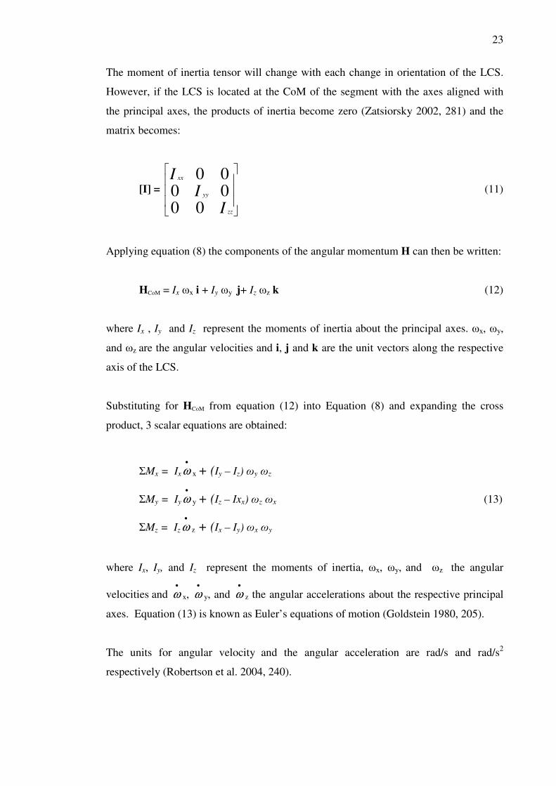
matrix becomes:

[I] =

II

I

zz

yy

xx

000000

(11)

Applying equation (8) the components of the angular momentum H can then be written:

HCoM = Ix ωx i + Iy ωy j+ Iz ωz k (12)

where Ix , Iy and Iz represent the moments of inertia about the principal axes. ωx, ωy,

and ωz are the angular velocities and i, j and k are the unit vectors along the respective

axis of the LCS.

Substituting for HCoM from equation (12) into Equation (8) and expanding the cross

product, 3 scalar equations are obtained:

ΣMx = Ix

•

ω x + (Iy – Iz) ωy ωz

ΣMy = Iy

•

ω y + (Iz – Ixx) ωz ωx (13)

ΣMz = Iz

•

ω z + (Ix – Iy) ωx ωy

where Ix, Iy, and Iz represent the moments of inertia, ωx, ωy, and ωz the angular

velocities and •

ω x, •

ω y, and •

ω z the angular accelerations about the respective principal

axes. Equation (13) is known as Euler’s equations of motion (Goldstein 1980, 205).

The units for angular velocity and the angular acceleration are rad/s and rad/s2

respectively (Robertson et al. 2004, 240).

24

3.1.5 Equations of motion: Angular kinematics

In order to obtain the angular velocity and angular acceleration of a segment, the

orientation of the segment with respect to time must be obtained. There are several

methods to calculate orientation of a segment such as direction cosines or the helical

technique (Zatsiorsky 1998, 25) but the most common is with the use of Euler angles

(Robertson et al. 2004, 52).

Euler angles are three angles that completely describe the orientation of one coordinate

system relative to another. These three angles can be described either geometrically or

by using three separate transformation matrices to rotate the local coordinate system

from the GCS to its actual orientation (Zatsiorsky 1998, 46). These rotations are

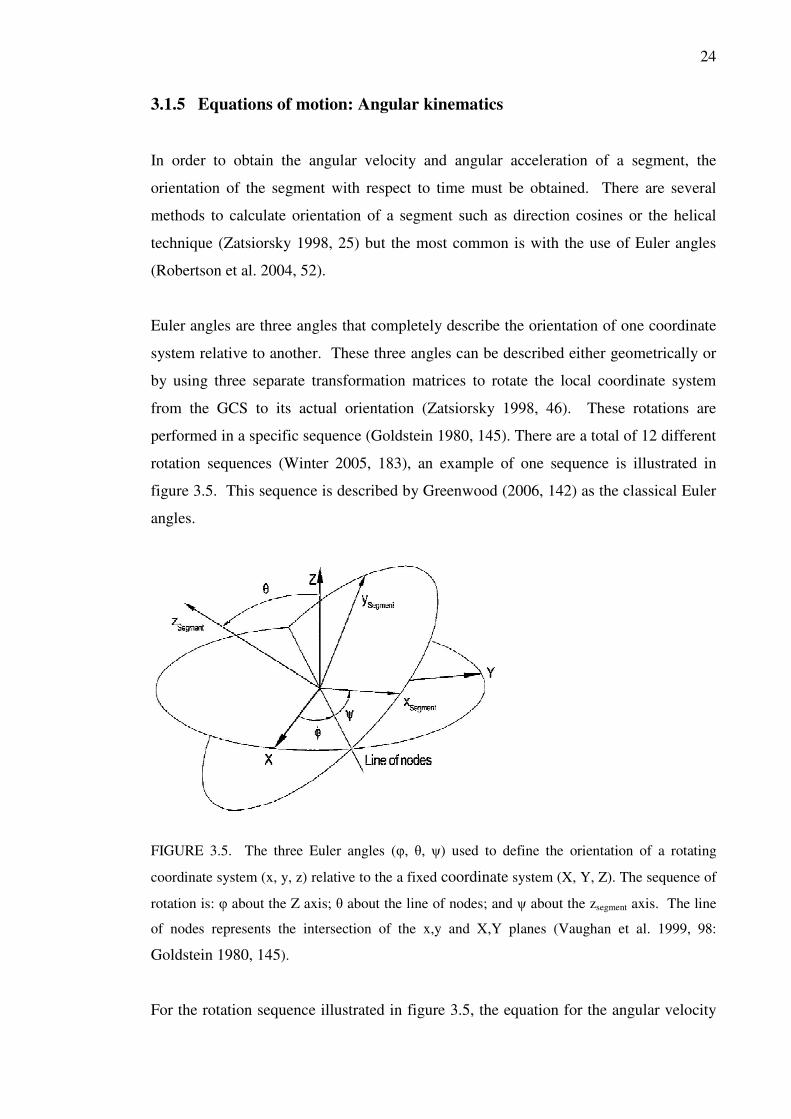
performed in a specific sequence (Goldstein 1980, 145). There are a total of 12 different

rotation sequences (Winter 2005, 183), an example of one sequence is illustrated in

figure 3.5. This sequence is described by Greenwood (2006, 142) as the classical Euler

angles.

FIGURE 3.5. The three Euler angles (φ, θ, ψ) used to define the orientation of a rotating

coordinate system (x, y, z) relative to the a fixed coordinate system (X, Y, Z). The sequence of

rotation is: φ about the Z axis; θ about the line of nodes; and ψ about the zsegment axis. The line

of nodes represents the intersection of the x,y and X,Y planes (Vaughan et al. 1999, 98:

Goldstein 1980, 145).

For the rotation sequence illustrated in figure 3.5, the equation for the angular velocity

25

about the local axes of the segment is given by (Goldstein 1980, 176):

+= ψθφω sinsin.&

xsegment ψθ cos&

ψθψθφω sincossin.&& −=ysegment (14)

ψθφω && += cos.zsegment

where the dot above the Euler angles represents the time derivative of the angle. The

derivation of the angular velocity equation (equation (13)) is given in the Appendix.

The segment angular accelerations can be calculated by taking the derivative of

equation (14) which gives the following (Vaughan et al 1999, 97):

ψψθψθψθψφψθθφψθφω sincoscossinsincossinsin.&&&&&&&&&&& −+++=xsegment

ψψθψθψθψφψθθφψθφω cossinsinsincoscoscossin.&&&&&&&&&&& −−−+=ysegment (15)

ψθθφθφω &&&&&&& +−= sincos.zsegment

where the double dot above the Euler angles represents the second time derivative of the

angle.

The derivation of the segment angular velocity and angular acceleration equations from

the Euler angles (equations (14) and (15)) is given in the Appendix.

The major disadvantage of the Euler angles is that errors in the calculation of the angles

will occur when the axes of the rotating system and the fixed system coincide. This is

known as gimbal lock (Zatsiorsky 1998, 52).

3.1.6 Limitations of the inverse dynamics model

Simplifications are a necessary part of the modelling process. For example, it is

assumed that each segment is non-deformable and has a fixed mass in the form of a

point mass located at its centre of mass (CoM) instead of mass unevenly distributed

along the whole segment. The location of CoM is assumed to remain fixed relative to

26

the segment during the movement. In reality, the movement of muscles and other soft

tissues would influence the CoM position. The mass moment of inertia of each segment

about its CoM is also assumed to remain constant. Also, all the joints are considered to

be frictionless ball and socket joints, free to move in all three planes (Kirtley 2006, 124;

Robertson et al. 2004, 116; Winter 2005, 87).

Inverse dynamic calculations for joint moments can only be performed when the CoP

can accurately be assessed to be under the foot of the performer. Due to limitations of

the force plates, when the vertical GRF is small (e.g. during the beginning and end of

the stance phase) the CoP calculation becomes unstable and will give erroneous CoP

locations (Robertson et al. 2004, 92).

3.2 Estimating muscle activity with the GRF vector

The ground reaction force vector (GRFV) can be used to give a simple indication of

which group of muscles are likely to be dominant when the foot is in contact with the

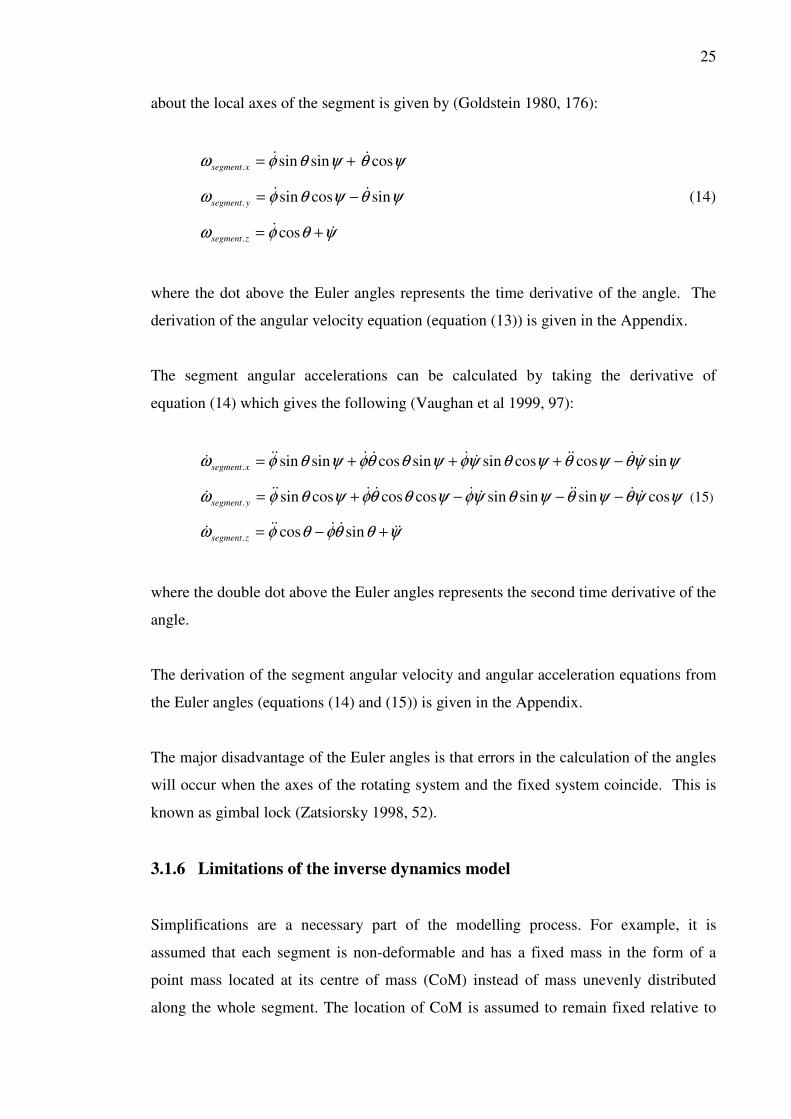
force plate (Kirtley 2006, 118). For example, for the ankle joint during quiet standing

(Figure 3.6) the ground reaction force is anterior to the ankle and would create an

external moment that would cause a dorsiflexor movement of the foot. To maintain

equilibrium, the Achilles tendon would need to produce an equal but opposite (internal)

moment (Newton’s third law). Therefore, the active muscle is likely to be on the

opposite side of the joint to the GRF (Kirtley 2006, 77).

GRF

Internal

momentExternal

moment

Achillestension

FIGURE 3.6. Balanced equilibrium between external and internal moments at the ankle joint

(Kirtley 2006, 77).

27

The same principle can be applied to the knee joint. For example, during a squatting

posture shown in figure 3.7, the GRFV passes posterior to the knee joint. This creates

an external moment that would cause the knee to flex. Therefore, the quadriceps

muscles are likely to be active to produce an internal extensor moment to maintain

equilibrium.

GRF

FIGURE 3.7. Diagram to show the position of the GRFV during squatting. The GRFV passes

anterior to the ankle joint and posterior to the knee joint.

Use of the GRFV to estimate muscle activity is also called the floor reaction force

vector approach (FRFV) in the literature (Simonsen et al. 1997). The FRFV approach

should not be used to calculate joint moments as it produces large errors in calculating

moments in joints that are superior to the ankle (Winter 2005, 105; Simonsen et al.

1997). However, it is used in clinical environments to provide instant qualitative

interpretation (Kirtley 2006, 120).

28

4 PURPOSE OF THE STUDY

The SS forehand has traditionally been taught as the main way of hitting the forehand

(Bollettieri 2001, 87). Although the OS forehand has previously been described as poor

technique and one that does not optimally utilise the kinematic chain of the lower body

(Bahamonde & Knudson 2003), it is the most common type of forehand in tennis today

(Roetert et al. 2009).

The advantages and disadvantages between the OS and SS forehands is a subject of

much debate amongst the coaching profession. One of the aspects has been knee joint

loading. In particular the loading of the left knee in the SS stroke has been stated as

being greater than that would be found in either knee in the OS (Langevad 2003).

However, to date, no data on the lower body kinetics of the OS and SS forehands have

been published. As a result of this, a scientific comparison of knee joint loading in the

OS and SS forehands has not been possible.

Therefore, the primary goal of this study was to calculate and compare the resultant

forces and moments of the knee joint in both the OS and SS forehand during both the

forward swing and follow-through phases. The hypothesis of this study was that the

greatest transverse plane moments in the knee joint would be found in the left knee of

the SS forehand during the follow-through phase.

An additional goal was to shed light on the role of the lower extremities in aiding pelvic

rotation, the latter being a critical process in the force generation of the forehand.

29

5 METHOD

5.1 Subjects

Seven male, right-handed university team level players (mean ± standard deviation, age

33 ± 11.5 years; mass 77.7 ± 14.2 kg) participated in the study. They all provided

informed consent. Each subject had 15 (2.5 cm diameter) spherical reflective markers

attached to the lower body as listed in table 5.1. In addition, 2 cm long strips of

reflective tape were placed on the tip and both sides of the subjects’ rackets.

TABLE 5.1. Names of the marker positions

Number Name

1

2

3

4

5

6

7

8

9 Left heel

10

11

12

13

14

15 Sacrum

Left anterior superior iliac spine (ASIS)

Right metatarsel head II

Right heel

Right lateral malleolus

Right tibial tubercle

Right femoral epicondyle

Right greater trochanter

Right anterior superior iliac spine (ASIS)

Left metatarsel head II

Left lateral malleolus

Left tibial tubercle

Left femoral epicondyle

Left greater trochanter

5.2 Experimental procedure and measurements

The experimental setup is shown in figure 5.1. The filming took place on an acrylic

indoor tennis court. Each subject performed OS and SS forehands with each foot on a

separate force plate (figure 5.2). The players were allowed to use their own rackets

during the data collecting process. As the surface of the force plates were 16.5 cm above

the court surface, a badminton net was fixed to the tennis net so it was 16.5 cm above

the normal height of the net. The tennis ball was fed via a tennis ball machine (Lobster

30

Elite III, Lobster, California, USA) at approximately 20 m/s. The subjects were

instructed to hit each ball with rally-paced ball speed and medium topspin over the

badminton net so that the ball would land into the 2.5 m by 2.5 m target area.

Y X

Z

Camera 1

Camera 2Camera 3

Camera 4

PC 1

PC 2

Synchronisation light

Global coordinate

system

Target area of the

tennis shot

Ball

machine

PC 3PC 3PC 3

FP Amplifier

AD board

Force p

late

2

(FP2)

Force p

late

1

(FP1)

Not to scale

α

α = 40°

FIGURE 5.1. The experimental setup showing the positions of the force plates, global

coordinate system, cameras and ball machine relative to the court.

Only the shot the subject decided represented a normal version of their forehand and

where the ball landed in the target zone was saved for later analysis. Altogether, three

OS and three SS forehands were saved for each subject. Four cameras were used. Two

cameras (Sony HDR-HC3 1080i, Sony, Japan) recorded at 200 frames per second (fps)

directly onto MiniDV tape whilst the other two cameras, (Memrecam fxK4 NAC)

recorded at 1000 fps onto laptop computers (PCs 1 and 2).

31

Z

Y

X

FIGURE 5.2. The picture shows a subject with one foot on each force plate, the location of the

markers and the global origin (X,Y,Z) located at the back right corner of force plate 1.

The outputs from the two force plates (Z13216, Kistler Instruments, Winterhur,

Switzerland) were amplified (Kistler 9861A) then converted to a digital signal (CED

DAC, CED Ltd. Oxford, UK) and recorded at 400Hz on a separate laptop (PC 3)

running Signal 2.16 program (CED Ltd). A pair of timing lights was used to help

synchronise the force plate data with the camera data. The lights were programmed to

flash twice during each shot, one short and one long flash. This was recorded along

with the force plate data on Signal 2.16.

An 8 rod, 25 point calibration frame (Peak Performance Technologies, Eaglewood, CO,

USA) of dimensions 2.2 m x 1.6 m x 1.9 m was filmed prior to and after each filming

session. The frame was large enough and was positioned on the force plates so that it

encompassed the space used by the players during their shots.

The subjects were weighed and lower body measurements were taken according to

figure 5.3.

32

FIGURE 5.3. The anthropometric measurements needed to calculate the masses and moments

of inertia of the six lower body segments (Vaughan et al 1999, 17). Since the subjects wore

tennis shoes, the foot model was modified to include the mass of the shoe.

5.3 Analytical procedures

The 25 points of the calibration frame were digitised using Vicon Motus 9.0 (Vicon

Motion Systems, Oxford, UK). The origin of the calibration frame was translated to the

back right corner of force plate 1 (as shown on figures 5.1 and 5.2) and the coordinate

system rotated using the Vicon Motus program.

One OS and one SS shot that was considered to be the closest to a text-book forehand

for each subject, was chosen for analysis. The markers were digitised using Vicon

Motus. This program uses the direct linear transformation method (Vicon User Manual)

to obtain the 3D coordinates of the markers using the information from the calibration

points. Since the filming was carried out by two pairs of different cameras filming at

different frame rates, the images from all cameras had to be processed to the same

camera speed (200 Hz). A short computer program was written for Avisynth 2.0 (free

open-source software) to deinterlace the images from the Sony cameras. The images

from the two Memrecam cameras were post-processed by a technician at the Finnish

Research Institute for Olympic Sports (KIHU) and recorded onto a digital video disc

(DVD).

33

The force plate data was imported into a specifically designed Excel (Microsoft

Corporation) template for processing. The force plate data was converted from volts

into Newtons and then the six GRF quantities were calculated (FX, FY, FZ, TZ, CoPX and

CoPY). The equations for computing the six quantities of the GRF are shown in table

5.2 (ISB, Kistler).

The scale factors were; FP1 37.3 mV/kg in the Z direction, FP2 35.8 mV/kg in the Z

direction, and 77.0 mV/kg in the X and Y directions for both plates. The force plate

data was recorded as voltages, therefore to convert it into Newtons; each sampled value

was multiplied by 1000, divided by the relevant scale factor and multiplied by 9.81

m/s2.

The final conversion involved translating and rotating the Kistler coordinate system to

the global coordinate system (GCS) used for the inverse dynamic computations. This

ensured the origin of the CoP was at the GCS origin and not at the centre of each plate.

Table 5.2. The equations used to calculate the ground reaction forces, CoP and vertical torque

(ISB Kistler).

Parameter Calculation Description*

Fx fx12 + fx34 Medial-lateral force ¹

Fy fy14 + fy23 Anterior force ¹

Fz fz1+fz2+fz3+fz4 Vertical force

Mx b*(fz1+fz2-fz3-fz4) Plate moment about X-axis ³

My a*(-fz1+fz2+fz3-fz4) Plate moment about Y-axis ³

Mz b*(-fx12+fx34)+a*(fy14-fy23) Plate moment about Z-axis ³

Mx' Mx+Fy*azO Plate moment about top plate surface ²

My' My-Fx*azO Plate moment about top plate surface²

CoP x -My'/Fz X-Coordinate of the centre of pressure ²

CoP y Mx'/Fz Y-Coordinate of the centre of pressure ²

Tz Mz-Fy*CoPx+Fx*CoPy Vertical torque

* Note, these parameters are in the Kistler coordinate system, not the GCS used for the inverse

dynamics calculations. ² azO = top plane offset (-0.08m). ³ sensor offset, a = 0.21m and b = 0.35m

Analysis of the obtained force-time graphs showed that the force plate data suffered

from varying amounts of drift, even though the reset button on the Kistler amplifier was

34

regularly pressed. This was rectified by finding when on the force-time curve the foot

was off the plate, and applying a correction factor for each of the 8 FP outputs. The

correction factor gave zero Newtons in all three directions (X,Y,Z) while the foot was

off the plate and a value of approximately ½ body weight during quite standing. This

enabled the force plates to be recalibrated after the data was collected. This was

performed on both force plates, for each subject and for every shot.

Further analysis of the CoP data revealed that the CoP data was not accurate enough for

the right leg of two subjects during the SS shot and so their right leg data was removed

from the analysis.

Certain calculations such as those shown in figures 6.2 and 6.3 in chapter 6, required the

positive axis for the medial/lateral ground reaction forces (GRFs) to be parallel to the

baseline pointing to the left and the positive axis for the anterior/posterior GRFs to be

perpendicular to the baseline in the direction of the net. The following formulae were

used to rotate the coordinate system of the force plates (ISB Kistler):

Fxlcs = (FX * cos 50) + (FY * sin 50) (16)

Fylcs = (FY * cos 50) – (FX * sin 50) (17)

where Fxlcs = anterior/posterior force, Fylcs = medial/lateral force. FX = force in the global X

direction, FY = force in the global Y direction as shown in figure (5.1) and figure (5.2).

Various computer programs were written using Matlab (The Mathworks,

Massachusetts, USA) in order to calculate the net lower body joint forces and torques.

The detailed mathematics of these calculations can be found in vector algebraic form in

Appendix B of Vaughan et al (1992) and Vaughan et al (1999).

Each lower limb was modelled as three rigid link segments of the foot, calf and thigh.

The free body diagram is shown in figure 3.2. In terms of the moments of inertia, the

calf and thigh were modelled as cylinders and the foot was modelled as a right pyramid.

The position of the centre of mass (CoM) of each segment relative to its proximal end

and the inertial properties of each segment were estimated using the coefficients and

regression equations of Vaughan et al (1999, 85).

35

The anatomical joint angles were determined according the convention adopted in the

joint coordinate system (JCS) of Grood and Suntay (1983). This enables the joint

angles to have a functional, anatomical meaning. Joint angles are defined as a rotation

of the distal segment relative to the proximal segment. An example of how the JCS is

defined for the knee is illustrated in figure 5.4. The rotations are defined as follows:

• Flexion and extension (plus dorsiflexion and plantar flexion) take place about

the mediolateral axis of the proximal segment (i.e., the kthigh axis)

• Internal and external rotation take place about the longitudinal axis of the distal

segment (i.e., the icalf axis).

• Abduction and adduction take place about a floating axis that is orthogonal to

both the flexion/extension and internal/external rotation axes.

icalf

kthigh

Floating axis

icalf

kcalf

jcalf

icalf

kcalf

jcalf

icalf

kcalf

jcalf

ithigh

kthigh

jthigh

ithigh

kthigh

jthigh

FIGURE 5.4. The JCS for the right knee. The axes are icalf , kthigh and the floating axis. The

floating axis is the cross product of these two axes. (Based on diagram in Robertson et al. 2004,

50).

The JCS gives a geometric description of the Cardan angles (Zatsiorsky 1998, 100) and

is the International Society of Biomechanics standard for reporting kinematic data

(Livesay et al. 1997).

36

The input for calculating segment linear acceleration was the CoM displacement data,

whereas the input for calculating segment angular velocity and angular acceleration

were the Euler angles. The order of rotation of the Euler angles was defined as: Z, line

of nodes, z (see figure 3.5 in chapter 3).

The equations given in the books by Vaughan et al (1992) and Vaughan et al (1999) for

calculating the Euler angles were used initially. However, polarity errors of the angular

velocities were found. These problems have also been identified by other researchers

(Ariel; Shen) using the books Dynamics of Human Gait by Vaughan et al (1992) and

(1999). Therefore, the following equations were used instead (Wikipedia):

φ = atan2 (kx, -ky) (18)

θ = cos-1

(kz) (19)

ψ = atan2 (iz, jz) (20)

where: i, j, k are the unit vectors of the segment in the global coordinate system and x,

y, z represent the x, y or z component of that unit vector, and atan2 is a standard

trigonomic computer function. An additional algorithm was used to ensure the polarity

of the angle was consistent.

The coordinate data for the markers, centre of mass (CoM) of each segment and the

segment Euler angles were smoothed using a 4th

order, zero phase lag Butterworth low-

pass digital filter (Winter 2005, 45). The cutoff frequency for each coordinate (X, Y

and Z) for each segment was determined individually by residual analysis (Winter 2005,

49).

The segment linear acceleration and the time derivatives of the Euler angles were

calculated using finite difference calculus (Robertson et al 2004, 21). The following

formulae were used:

( )t

xxx

dt

dx nn

n

n

∆

−== −+

2

11& (21)

37

( )2

11

2

2 2

t

xxxx

dt

xd nnn

n

n

∆

+−== −+

&& (22)

where x is an input data point, n refers to the nth sample and ∆t is the time between

adjacent frames. Velocity was calculated using equation (21) and acceleration using

equation (22).

The segment angular velocities and angular acceleration were calculated from equations

(14) and (15) respectively. The segment angular velocities and angular accelerations

were then used along with the segment inertia parameters and the moments created from

the joint reaction forces, as inputs into equation (13) for calculating the net moment

acting on a segment.

To aid in comparison of the results, the net forces and moments were normalised and

the stroke was divided into two temporal phases. The net joint reaction forces were

normalised by divided by body weight and multiplied by 100%, and the net joint

moments were normalised by dividing my body mass. This is a standard way of

normalising gait analysis data (Kirtley 2005, 127; Allard et al. 1997, 315). The

temporal phases of the stroke were termed forward swing and follow-through. These

were defined as:

• Forward swing: from the beginning of trunk left rotation to impact.

• Follow-through: from ball impact to the point were the trunk had stopped

rotating.

The force plate readings (particularly the centre of pressure) became unreliable when

the vertical force was below approximately 10% body weight. The amount varied

depending on the subject and the shot. This was most noticeable for the right leg both

during and after impact with the ball when the vertical components were at their lowest

as the weight was now over the front foot. The individual subjects’ resultant moments

were not analysed when the CoP could not be accurately assessed to be under the

subject’s foot. That is why no kinetic data has been recorded in tables 6.4 to 6.7 and

figure 6.8 for the right leg during the follow-through phase.

38

5.4 Expression of joint forces and moments

The resultant joint reaction forces and joint moments are expressed in terms of the axes

used in describing the JCS. These are defined as follows (Vaughan et al 1999, 41):

Forces

• A mediolateral force takes place along the mediolateral axis of the proximal

segment.

• A proximal/distal force takes place along the longitudinal axis of the distal

segment.

• An anterior/posterior force takes place along a floating axis that is perpendicular

to the mediolateral and longitudinal axes.

Moments

• A flexion/extension moment takes place about the mediolateral axis of the

proximal segment.

• An internal/external rotation moment takes place about the longitudinal axis of

the distal segment.

• An abduction/adduction moment takes place about a floating axis that is

perpendicular to the mediolateral and longitudinal axes.

In should be noted the axes used in the JCS are defined relative to the body segments

and therefore, are not necessarily in the same directions as the force plate axes. Also,

the JCS is not an orthogonal system (Zatsiorsky 1998, 101) the resultant forces and

moments at each joint may not be exactly at right angles to each other.

5.5 Statistical Methods

Statistical analysis was performed using Matlab. The data was first tested for normality

using the Kolmogorov-Smirnov (K-S) test. The data failed this test and so significance

testing was performed using the non-parametric Wilcoxon matched pairs test instead of

the t test. The statistical significance was set at a level of p≤0.05.

39

Only when there was sufficient reliable data from all seven subjects were the results

statistically analysed. This means that no statistical analysis was performed on the right

knee for the SS shot and for the right knees in the follow-through phase of both strokes.

40

6 RESULTS

6.1 Stroke parameters

In order to assess whether the biomechanical parameters of the OS and SS strokes were

easily comparable with each other, racket speed, ball velocity and normalised ball

height at impact were analysed.

The mean resultant racket tip speed just before ball impact for the OS and SS strokes

were 28.45 ± 2.27 m/s and 29.25 ± 1.5 m/s, respectively. These were not significantly

different (n.s.). The mean resultant ball speed just prior to impact in the OS and SS

strokes were 7.54 ± 0.22 and 7.76 ± 0.24 m/s, respectively (n.s.). The average forward

swing times of the OS and SS strokes were 0.22 ± 0.03 and 0.24 ± 0.04 s, respectively

(n.s.). The mean ratio of ball impact height to the height of the right hip at impact for

the OS and SS strokes were 1.10 ± 0.13 and 0.96 ± 0.15, respectively (n.s.).

6.2 Ground reaction forces

As the GRF reflects the summation of the mass acceleration products of all body

segments, some of the fundamental differences between the OS and SS techniques can

be seen in the recorded GRFs.

6.2.1 Weight transfer

Typical examples of the vertical ground reaction forces (Fz) as a function of time in the

OS and SS strokes are shown in figures 6.1a and 6.1b. These figures clearly show the

transfer of body weight from the right leg to the left leg. This was observed for all

participants in both the OS and SS strokes. The difference was in the timing of the

weight transfer. For all subjects except one, the weight transfer occurred after contact

in the OS forehand. In the SS forehand, the weight transfer occurred before contact for

all subjects.

41

Open Stance

0

200

400

600

800

1000

1200

-0,5 -0,4 -0,3 -0,2 -0,1 0 0,1 0,2 0,3

Time (s)

GR

F (

N)

Fz Left

Fz Right

Open Stance

0

200

400

600

800

1000

1200

-0,5 -0,4 -0,3 -0,2 -0,1 0 0,1 0,2 0,3

Time (s)

GR

F (

N)

Fz Left

Fz Right

Square Stance

0

200

400

600

800

1000

1200

-0,5 -0,4 -0,3 -0,2 -0,1 0 0,1 0,2 0,3

Time (s)

GR

F (

N)

Fz Left

Fz Right

Square Stance

0

200

400

600

800

1000

1200

-0,5 -0,4 -0,3 -0,2 -0,1 0 0,1 0,2 0,3

Time (s)

GR

F (

N)

Fz Left

Fz Right

a) b)

Open Stance

-30

-20

-10

0

10

20

30

40

-0,5 -0,4 -0,3 -0,2 -0,1 0 0,1 0,2 0,3

Time (s)

To

rqu

e (

Nm

)

Tz Left

Tz Right

Open Stance

-30

-20

-10

0

10

20

30

40

-0,5 -0,4 -0,3 -0,2 -0,1 0 0,1 0,2 0,3

Time (s)

To

rqu

e (

Nm

)

Tz Left

Tz Right

Square Stance

-30

-20

-10

0

10

20

30

40

-0,5 -0,4 -0,3 -0,2 -0,1 0 0,1 0,2 0,3

Time (s)T

orq

ue (

Nm

)

Tz Left

Tz Right

Square Stance

-30

-20

-10

0

10

20

30

40

-0,5 -0,4 -0,3 -0,2 -0,1 0 0,1 0,2 0,3

Time (s)T

orq

ue (

Nm

)

Tz Left

Tz Right

c) d)

Figure 6.1. The vertical ground reaction forces (Fz), figures a and b, and vertical torques (Tz),

figures c and d for one representative subject. Positive values reflect a counter-clockwise

torque. Negative values reflect a clockwise torque. Time zero = ball contact.

6.2.2 Vertical torque

The vertical torque (TZ) applied to the feet about the vertical Z axis as a function of time

in the OS and SS strokes is shown in figures 6.1c and 6.1d. Maximum values for the

vertical torque were recorded before contact in the right leg in the OS forehand and after

contact in the left leg in the SS forehand. The values for the mean peak vertical torque

are shown in table 6.1. The mean peak vertical torque in the OS right leg prior to

impact, 0.27 ± 0.09 Nm/kg was significantly greater than the SS left leg follow-through,

0.17 ± 0.07 Nm/kg (p=0.016). The total torque generated (i.e. the range) by the right leg

in the OS was nearly significantly greater than the left leg in the SS (p=0.078).

42

TABLE 6.1. The normalised mean peak vertical torque (Tz) applied to the sole of the tennis

shoe. CW = clockwise torque, CCW = counter clockwise torque.

Open Stance (OS) Nm/kg ± (standard dev.)

Foot CW Torque CCW Torque Range

Left 0.07 (0.04) 0.11 (0.06) 0.18 (0.08)

Right 0.05 (0.03) 0.27 (0.09) 0.32 (0.11)

Square Stance (SS)

Foot CW Torque CCW Torque Range

Left 0.17 (0.07) 0.09 (0.03) 0.26 (0.08)

Right 0.13 (0.05)5

0.10 (0.09)5

0.23 (0.07)5

( )n = number of subjects (if n < 7).

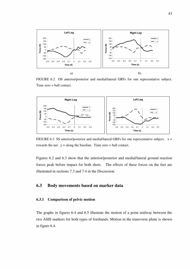
6.2.3 Medial/lateral and anterior/posterior GRFs

The GRFs in the anterior/posterior and medial/lateral directions in both types of shot for

the same subject are shown in figures 6.2 and 6.3. The anterior/posterior direction (x) is

at right angles to the baseline pointing towards the net. The medial/lateral direction (y)

is parallel to the baseline pointing to the left.

43

Left Leg

-150

-100

-50

0

50

100

150

200

-0,5 -0,4 -0,3 -0,2 -0,1 0 0,1 0,2 0,3

Time (S)

Fo

rce

(N

)x

y

Right Leg

-150

-100

-50

0

50

100

150

200

-0,5 -0,4 -0,3 -0,2 -0,1 0 0,1 0,2 0,3

Time (s)

Fo

rce

(N

)

x

y

Right Leg

-150

-100

-50

0

50

100

150

200

-0,5 -0,4 -0,3 -0,2 -0,1 0 0,1 0,2 0,3

Time (s)

Fo

rce

(N

)

x

y

a) b)

FIGURE 6.2 OS anterior/posterior and medial/lateral GRFs for one representative subject.

Time zero = ball contact.

Right Leg

-150

-100

-50

0

50

100

150

200

-0,5 -0,4 -0,3 -0,2 -0,1 0 0,1 0,2 0,3

Time (s)

Fo

rce (N

)

x

y

Right Leg

-150

-100

-50

0

50

100

150

200

-0,5 -0,4 -0,3 -0,2 -0,1 0 0,1 0,2 0,3

Time (s)

Fo

rce (N

)

x

y

Left Leg

-150

-100

-50

0

50

100

150

200

-0,5 -0,4 -0,3 -0,2 -0,1 0 0,1 0,2 0,3

Time (s)

Fo

rce

(N

) x

y

Left Leg

-150

-100

-50

0

50

100

150

200

-0,5 -0,4 -0,3 -0,2 -0,1 0 0,1 0,2 0,3

Time (s)

Fo

rce

(N

) x

y

FIGURE 6.3 SS anterior/posterior and medial/lateral GRFs for one representative subject. x =

towards the net. y = along the baseline. Time zero = ball contact.

Figures 6.2 and 6.3 show that the anterior/posterior and medial/lateral ground reaction

forces peak before impact for both shots. The effects of these forces on the feet are

illustrated in sections 7.3 and 7.4 in the Discussion.

6.3 Body movements based on marker data

6.3.1 Comparison of pelvic motion

The graphs in figures 6.4 and 6.5 illustrate the motion of a point midway between the

two ASIS markers for both types of forehands. Motion in the transverse plane is shown

in figure 6.4.

44

0,65

0,75

0,85

0,95

1,05

1,15

-0,3-0,2-0,100,10,2

Along the base line (m)

To

ward

s t

he n

et

(m)

Open Stance

Square Stance

Position at contact

Net

Baseline

FIGURE 6.4. Transverse view of the motion of the midpoint between the ASIS markers during

one complete OS and SS stroke for one representative player.

The mean horizontal translation of the midpoint towards the net, for OS and SS in the

0.5 s prior to impact were 11.4 ± 6.5 cm and 29.2 ± 5.8 cm, respectively. This was

significantly different (p=0.016).

Pelvic angular velocity. There was no significant difference between the average peak

transverse plane angular velocity of the pelvis in the OS and SS strokes during the

forward swing phase (5.54 ± 1.10 rad/s and 5.02 ± 1.56 rad/s respectively).

Vertical motion of the pelvis. The vertical motion (along the global Z-axis) of the

midpoint between the two ASIS markers as function of time for the two types of

forehands is shown in figure 6.5. The mean maximum vertical translation of the

midpoint for OS and SS during the forward swing was 12.0 ± 3.0 cm and 6.9 ± 3.0 cm,

respectively. This was significantly different (p=0.016).

-0.5 -0.4 -0.3 -0.2 -0.1 0 0.1 0.2 0.30.9

0.95

1

1.05

1.1

1.15

Time (s)

He

igh

t o

f m

idp

oin

t b

etw

ee

n t

he

AS

IS m

ark

ers

(m

)

Open Stance

Square Stance

FIGURE 6.5. Illustration of the vertical motion of the midpoint between the ASIS markers.

Data from two different players. Time zero = ball contact.

45

6.3.2 Knee angles

Maximum knee flexion occurred at the start of the forward swing phase which was

followed by extension towards impart. There were no significant differences between

the maximum knee flexion angles in the two strokes (table 6.2). Although, on average,

the amount of right knee extension before impact was greater for the OS, there was also

no significant difference in the amount of knee extension recorded from maximum knee

flexion to ball impact (table 6.3).

Table 6.2 Maximum joint angles of the knees. Data is presented as mean (degrees) ± (standard

dev.)

Open Stance (OS) Square Stance (SS)

Left Knee 61.9 (±13.7) 53.9 (±14.3)

Right Knee 47.4 (±14.9) 42.6 (±15.8)

Table 6.3. Amount of knee extension from maximum flexion to ball impact. Data is presented

as mean (degrees) ± (standard dev.)

Open Stance (OS) Square Stance (SS)

Left Knee 27.3 (±4.1) 26.1 (±9.1)

Right Knee 36.2 (±8.6) 22.0 (±10.3)

6.3.3 Peak knee external rotation moment versus knee flexion angle

There was, however, a difference between the knee flexion angles when the peak

external rotation moment occurred. The mean OS right knee and SS left knee flexion

angles were 49.5 degrees (±13.2) and 19 (±4.2) degrees respectively, p=0.031. This

indicates that the peak external rotation moments occur with the knee in a more

extended position in the SS follow-through.

46

6.4 Forces and moments of the knee joint

6.4.1 Open stance

Typical examples of the resultant reaction forces and moments for the knee as a

function of time in the OS stroke are shown in figure 6.6.

-0.4 -0.2 0 0.2-1000

-500

0

500

Time (s)

Fo

rce (

N)

Forces Left Knee

Prx/Dis

Med/Lat

Ant/Pos

-0.4 -0.2 0 0.2-1000

-500

0

500

Time (s)

Fo

rce (

N)

Forces Right Knee

-0.4 -0.2 0 0.2

-100

-50

0

50

100

150

Time (s)

Mo

men

t (N

m)

Moments Left Knee

Flx/Ext

Abd/Add

Int/Ext

-0.4 -0.2 0 0.2

-100

-50

0

50

100

150

Time (s)

Mo

men

t (N

m)

Moments Right Knee

-0.4 -0.2 0 0.2-1000

-500

0

500

Time (s)

Fo

rce (

N)

Forces Left Knee

Prx/Dis

Med/Lat

Ant/Pos

-0.4 -0.2 0 0.2-1000

-500

0

500

Time (s)

Fo

rce (

N)

Forces Right Knee

-0.4 -0.2 0 0.2

-100

-50

0

50

100

150

Time (s)

Mo

men

t (N

m)

Moments Left Knee

Flx/Ext

Abd/Add

Int/Ext

-0.4 -0.2 0 0.2

-100

-50

0

50

100

150

Time (s)

Mo

men

t (N

m)

Moments Right Knee

FIGURE 6.6. OS forces and moments for one representative subject. Positive values

correspond to proximal, medial and anterior forces and flexion, abduction and internal rotation

moments. Negative values correspond to distal, lateral and posterior forces and extension,

adduction and external rotation moments. Time zero = ball contact. For the period when the foot

was off the force plate, no moments were calculated.

Forces. Table 6.4 lists the average maximum normalised knee joint reaction forces

recorded during the forward swing and follow-through phases. The dominant knee

force was the distal (weight bearing) force. In the forward swing phase, the greatest

distal forces were found in the right knee (p=0.014), whereas, in the follow-through,

greater distal forces were found in the left knee. During the beginning of the forward

swing phase the right knee distal, lateral and anterior forces all reached their peak. In

the left knee the anterior and distal forces were of similar magnitude during the forward

swing. The anterior force peaked during the forward swing phase; the distal force

peaked during the follow-through.

47

TABLE 6.4. Average maximum knee forces recorded during the forward swing and follow-

through phases for the OS forehand. Data is represented as maximum force (F) divided by body

weight (BW).

FORWARD SWING F/BW (%) [± standard dev.]

Prox Dist Med Lat Ant Pos

Left Knee NSD 36.8 (±28.2)* 6.7 (±5.6) NSD 39.6 (±13.5) NSD

Right Knee NSD 104.5 (±25.8) NSD 14.4 (±8.8) 24.0 (±16.1) NSD

FOLLOW-THROUGH

Prox Dist Med Lat Ant Pos

Left Knee NSD 71.2 (±21.7) NSD 4.7 (±2.7) 14.5 (±7.3)6

7.8 (±2.9)5

Right Knee NSD NSD NSD NSD NSD NSD

NSD = Not sufficient data (data for less than 4 subjects), n Number of subjects (if not seven).

* Significantly less than the value for the same knee in the SS stroke.

Moments. The largest knee moments (in decreasing order of magnitude) were

flexion/extension, abduction and external rotation (table 6.5). The greatest moments

were left knee extension moments which peaked during the forward swing for all

subjects. During the forward swing phase six subjects displayed both extension

followed by flexion moments in the right knee. One subject only showed a flexion

moment for the right knee. The right knee abduction moments peaked during the

forward swing phase, while the left knee abduction moments peaked during the follow-

through. The major transverse plane moments were right knee external rotation which

peaked at the start of the forward swing phase (figure 6.8b).

TABLE 6.5. Average maximum knee moments recorded during the forward swing and follow-

through phases for the OS forehand.

FORWARD SWING Nm/kg (± standard dev.)

Flex Ext Abd Add Int Rot Ext Rot

Left Knee NSD 1.46 (±0.53) 0.2 (±0.17)▲

0.23 (±0.10)6 0.14 (±0.07) 0.05 (±0.07)

●

Right Knee 0.55 (±0.29) 0.71 (±0.43)6 0.33 (±0.14)6NSD NSD 0.24 (±0.13)

FOLLOW-THROUGH

Flex Ext Abd Add Int Rot Ext Rot

Left Knee 0.54 (±0.26)6NSD 0.32 (±0.16)

♦NSD NSD 0.10 (±0.09)

■

Right Knee NSD NSD NSD NSD NSD NSD

NSD = Not sufficient data (data for less than 4 subjects), n Number of subjects (if not seven).

♦■●▲ Significantly less than the value for the same knee in the SS stroke

48

6.4.2 Square stance

Typical examples of the resultant reaction forces and moments for the knee as a

function of time in the SS stroke are shown in figure 6.7.

-0.4 -0.2 0 0.2-1000

-500

0

500

Time (s)

Forc

e (N

)

Forces Left Knee

Prx/Dis

Med/Lat

Ant/Pos

-0.4 -0.2 0 0.2-1000

-500

0

500

Time (s)

Forc

e (N

)

Forces Right Knee

-0.4 -0.2 0 0.2

-100

-50

0

50

100

150

Time (s)

Mom

ent (N

m)

Moments Left Knee

Flx/Ext

Abd/Add

Int/Ext

-0.4 -0.2 0 0.2

-100

-50

0

50

100

150

Time (s)

Mom

ent (N

m)

Moments Right Knee

-0.4 -0.2 0 0.2-1000

-500

0

500

Time (s)

Forc

e (N

)

Forces Left Knee

Prx/Dis

Med/Lat

Ant/Pos

-0.4 -0.2 0 0.2-1000

-500

0

500

Time (s)

Forc

e (N

)

Forces Right Knee

-0.4 -0.2 0 0.2

-100

-50

0

50

100

150

Time (s)

Mom

ent (N

m)

Moments Left Knee

Flx/Ext

Abd/Add

Int/Ext

-0.4 -0.2 0 0.2

-100

-50

0

50

100

150

Time (s)

Mom

ent (N

m)

Moments Right Knee

FIGURE 6.7. SS forces and moments for one representative subject. Positive values

correspond to proximal, medial and anterior forces and flexion, abduction and internal rotation

moments. Negative values correspond to distal, lateral and posterior forces and extension,

adduction and external rotation moments. Time zero = ball contact.

Forces. Table 6.6 lists the average maximum normalised knee joint reaction forces

recorded during the forward swing and follow-through phases. The major right leg

force was distal which decreased during the forward swing phase reducing to close to

zero during the follow-through. The right knee medial/lateral forces moved from lateral

at the beginning of the forward swing to medial just before ball impact. Greater

medial/lateral and anterior/posterior forces were found in the left knee. The left knee

distal force reached its peak during the follow-through. The anterior forces peaked

during the forward swing phase. Medial forces were present in the left knee at the

beginning of the forward swing phase which turned to lateral forces just before ball

impact for all subjects

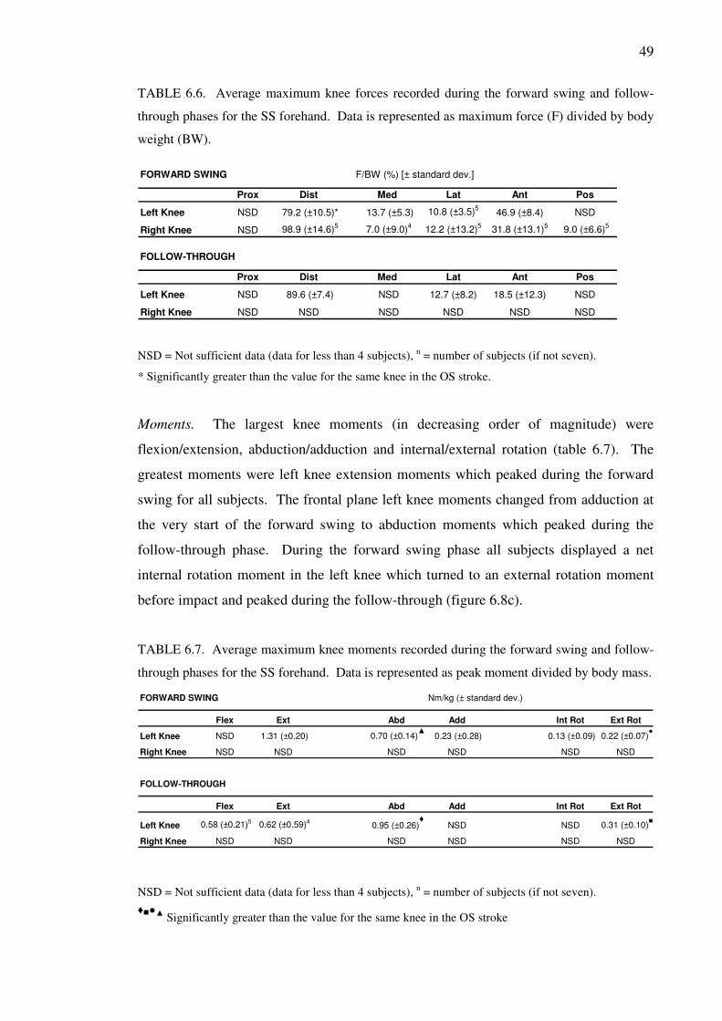
49

TABLE 6.6. Average maximum knee forces recorded during the forward swing and follow-

through phases for the SS forehand. Data is represented as maximum force (F) divided by body

weight (BW).

FORWARD SWING F/BW (%) [± standard dev.]

Prox Dist Med Lat Ant Pos

Left Knee NSD 79.2 (±10.5)* 13.7 (±5.3) 10.8 (±3.5)5

46.9 (±8.4) NSD

Right Knee NSD 98.9 (±14.6)5

7.0 (±9.0)4

12.2 (±13.2)5

31.8 (±13.1)5

9.0 (±6.6)5

FOLLOW-THROUGH

Prox Dist Med Lat Ant Pos

Left Knee NSD 89.6 (±7.4) NSD 12.7 (±8.2) 18.5 (±12.3) NSD

Right Knee NSD NSD NSD NSD NSD NSD

NSD = Not sufficient data (data for less than 4 subjects), n = number of subjects (if not seven).

* Significantly greater than the value for the same knee in the OS stroke.

Moments. The largest knee moments (in decreasing order of magnitude) were

flexion/extension, abduction/adduction and internal/external rotation (table 6.7). The

greatest moments were left knee extension moments which peaked during the forward

swing for all subjects. The frontal plane left knee moments changed from adduction at

the very start of the forward swing to abduction moments which peaked during the

follow-through phase. During the forward swing phase all subjects displayed a net

internal rotation moment in the left knee which turned to an external rotation moment

before impact and peaked during the follow-through (figure 6.8c).

TABLE 6.7. Average maximum knee moments recorded during the forward swing and follow-

through phases for the SS forehand. Data is represented as peak moment divided by body mass.

FORWARD SWING Nm/kg (± standard dev.)

Flex Ext Abd Add Int Rot Ext Rot

Left Knee NSD 1.31 (±0.20) 0.70 (±0.14)▲

0.23 (±0.28) 0.13 (±0.09) 0.22 (±0.07)●

Right Knee NSD NSD NSD NSD NSD NSD

FOLLOW-THROUGH

Flex Ext Abd Add Int Rot Ext Rot

Left Knee 0.58 (±0.21)5 0.62 (±0.59)4 0.95 (±0.26)

♦NSD NSD 0.31 (±0.10)

■

Right Knee NSD NSD NSD NSD NSD NSD

NSD = Not sufficient data (data for less than 4 subjects), n = number of subjects (if not seven).

♦■●▲ Significantly greater than the value for the same knee in the OS stroke

50

6.4.3 Internal/external rotation moments

Since the temporal phase patterns of internal and external rotation moments for all

subjects were very similar, an ensemble average curve could be plotted. The average

curve profiles of the transverse plane knee moments during the OS and SS forehands for

all subjects are shown in figures 6.8a, 6.8b and 6.8c respectively. In the left knee for

both the OS and SS strokes, all subjects had a similar pattern of internal rotation

(positive peak) before ball impact and an external rotation moment (negative peak) after

impact.

OS Left Leg

-0,3

-0,2

-0,1

0

0,1

0,2

-0,4 -0,2 0 0,2 0,4

Time (s)

Tra

nsvers

e P

lan

e M

mo

men

t

(Nm

/kg

)

OS Right Leg

-0,3

-0,2

-0,1

0

0,1

0,2

-0,4 -0,2 0 0,2 0,4

Time (s)

Tra

nsvers

e P

lan

e M

om

en

t

(Nm

/kg

)

a) b)

SS Left Leg

-0,3

-0,2

-0,1

0

0,1

0,2

-0,4 -0,2 0 0,2 0,4

Time (s)

Tra

ns

ve

rse

Pla

ne

Mo

me

nt

(Nm

/kg

)

c)

FIGURE 6.8. Left and right knee average transverse plane moment profile (7 subjects). a) OS

left knee b) OS right knee and c) SS left knee. Positive values correspond to internal rotation

moments. Negative values correspond to external rotation moments. Time zero = ball contact.

In the right knee for the OS stroke, all subjects had a similar pattern of external rotation

(negative peak) before ball impact (figure 6.8b).

51

Since the location of the CoP was inconsistent for most subjects for the right force plate

during the OS follow-through and SS forward swing and follow-through, it was not

possible to produce a coherent average plot for the SS right knee. This was because

most of the weight had been transferred to the left leg at the beginning of the forward

swing phase.

6.4.4 Kinetic comparison of the open stance and square stance strokes

Forces. The left knee distal force was greater for the SS in the left leg during the

forward swing phase (79.2 ±10.5 % BW) compared to the left leg in the OS forward

swing phase (36.8 ±28.2 % BW), (p=0.016). No differences were found between the

OS and SS left knee medial forces in the forward swing phase. No differences were

found between the OS and SS left knee anterior forces in the forward swing phase.

During the follow-through, there was a trend for the lateral forces in the SS left knee

(12.7 ±8.2 % BW), to be greater than the OS left knee (4.7 ±2.7 % BW), which

approached significance (p=0.063). No differences were found when comparing the left

knee distal forces in the follow-through.

Moments. There was a greater abduction moment in the left knee in the SS forward

swing phase (0.70 ±0.14 Nm/kg) compared with the left knee in the OS forward swing

phase (0.20 ±0.17 Nm/kg), (p=0.016). There was also a greater abduction moment in

the left knee in the SS follow-through stage (0.95 ±0.26 Nm/kg) compared to the left

knee in the OS follow-through (0.32 ±0.16 Nm/kg), (p=0.016). The largest moments in

the transverse plane were the external rotation moments of the left knee in the SS follow

through. The external rotation moments in the left knee were significantly greater in the

SS stroke than the OS stroke during both the forward swing (0.22 ±0.07 Nm/kg)

compared with (0.05 ±0.07 Nm/kg), respectively (p=0.016) and the follow-through

phases (0.31 ±0.10) compared to (0.10 ±0.09), respectively (p=0.031). This can be seen

from the average curves in figure 6.8. However, there was no significant difference

between the right knee OS external rotation moment in the forward swing phase (0.24

±0.13 Nm/kg) when compared with the SS left knee external rotation moment of the

follow-through (0.31 ±0.10 Nm/kg), (p=0.30).

52

7 DISCUSSION

The primary purpose of this study was to calculate and compare the reaction forces and

moments of the knee joint in the OS and SS tennis forehand.

The main findings of this study were: (a) the largest abduction moments occurred in the

left knee of the SS stroke during the follow-through. (b) The largest external rotation

moments were found in the SS left knee during the follow-through and in the OS right

knee prior to impact. (c) The peak OS external rotation moment occurred with the right

knee in a more flexed position compared to the SS left knee peak external rotation

moment. (d) The greatest peak ground reaction torque (TZ) was generated by the right

leg in the OS stroke before impact.

As there was no significant difference between the right knee OS external rotation

moment in the forward swing phase when compared with the SS left knee external

rotation moment of the follow-through, the research hypothesis was rejected.

It was expected that the greatest external rotation moments would be found in the left

knee during the follow-through phase of the SS stroke. The fact that the OS generates a

similar level of external rotation moment in the right knee in the forward swing phase

was not expected initially. Although, considering that the OS does not use any initial

forward stepping action before impact, it is reasonable that the right knee external

rotation moment could have an important role in assisting pelvic rotation.

7.1 Stroke parameters

The obtained results show that in terms of angular velocity of the pelvis, racket head

speed, ball speed, swing time and ratio of ball impact height; there were no significant

differences between the two strokes. This means that the differences between the two

strokes were likely to be due to the differences in the technique and not because of

differences in for example, how fast the subjects swung the racket.

53

7.2 Comparison with the literature

In order to evaluate the validity of the kinetic and other data values obtained in this

study, a comparison was made with the values found in the literature. As very little

relevant tennis data exists, data from other sports with similar type of movement

patterns was used.

Knee moments. A comparison of the knee moments found in this study and those

reported in the literature for similar types of athletic movements is shown in table 7.1.

TABLE 7.1. Comparison between mean peak moments experienced by the knee during the

tennis forehand, golf, walking, running, a running side step manoeuvre and baseball pitching.

Peak Knee Moment Nm/kg (± standard dev.)

Extension Abduction External Rotation

Activity Moment Moment Moment

Tennis (SS Left Knee) 1.31 (0.20) 0.95 (0.26) 0.31 (0.10)

Tennis (CS Left Knee)a

1.0 (0.26)

Tennis (OS Right Knee) 0.71 (0.43) 0.33 (0.14) 0.24 (0.13)

Golf (Lead Knee)b

1.26 0.83 0.36

Golf (Trail Knee)b

0.25

Golf (Lead Knee)c

0.54 (0.25)

Walkingd

0.2 0.3 0.15

Running (3.2 m/s)e

0.4 0.7 0.23

Running side-step (60o)f

2.2 0.2 0.32

Baseball Pitching (Lead Knee)g

1.00

Baseball Pitching (Trail Knee)g

0.95

a = Iino and Kojima 2003, b = Gatt et al. (1999, 20), c = Lynn and Noffal (2010), d = Allard

(1997, 315), e = Kerrigan et al. 2009, f = Besier et al. (2001), and g = Huang and Lin (2011).

Values in bold refer to the present study.

The average maximum extension moment found in this study in the SS left knee was

slightly greater than that reported by Iino and Kojima (2003) for the closed stance

forehand, although the mean resultant racket speeds described in their article and in this

study were similar, 28.2 ±3.3 and 29.2 ±1.5 m/s respectively.

54

No published data for the abduction moment of the knee of the tennis forehand was

found. However, when compared to data for similar types of movements in other

sports, the values obtained for the maximum abduction moment in the leading knee of

the SS in this study were similar to those reported for the leading knee in baseball

pitching but greater than those reported for walking and running.

The peak external rotation moments found in the tennis shots are similar to those

calculated for a golf drive and running sidestep manoeuvre, but are slightly greater than

the peak external rotation moments reported in walking and running.

Weight transfer. The timing of the observed weight transfer for both the OS and SS

strokes was consistent with the descriptions of proper technique found in coaching texts

and previous research on the OS and SS forehand (Bahamonde & Knudson 2003). As

noted in section 2.1.1 and 2.1.2.

Vertical torque. Force plate torque values for sports techniques are rarely reported in

the literature (Lees & Lake 2008, 65; Miller 1990, 220). The mean peak force plate TZ

values for the right leg (Table 6.1) in the OS are similar to those reported for the leading

leg in golf (0.27 Nm/kg) using metal spiked shoes (Worsfold et al. 2008).

Anterior/posterior ground reaction forces. The anterior/posterior ground reaction

forces for the SS forehand shown in figure 6.3 agree with the propulsion followed by

braking prior to impact forces illustrated by van Gheluwe and Hebbelinck (1986) and

Iino and Kojima (2001) shown in section 2.1.3.

Knee flexion angles. The maximum flexion angles of the left and right knees of 42.6°

and 53.9° in the SS stroke were similar to the flexion angles of the left and right knees

of 50.2° and 54.7°, respectively, reported by and Iino and Kojima (2003) for the CS

forehand.

Conclusion. Comparison with the literature has shown that the range of the data values

obtained in this study were at a reasonable level. Although, the mean peak values are

similar to those found in golf and the external rotation moment was lower than that

55

found in the trail knee in baseball pitching, the injury risk of tennis compared to these

sports is not so clear. In tennis, more forehands are likely to be hit during a normal

match than one would execute the drive in golf or pitch a baseball during a normal

game of these respective sports.

7.3 Open stance forces and moments

Since there is no published data concerning OS knee forces and moments it is not

possible to directly compare the OS results with previous studies. Therefore, only an

indirect comparison can be made with actions from other aspects of human motion.

The loading of the knee joint corresponds with the flexion and extension of the knee and

the location of the player's weight. During the backswing phase the players first flexed

their knees with the majority of the weight over the right leg for 6 of the 7 subjects.

During the flexion the right force plate torque and right knee forces increased. At

approximately 0.2 seconds before ball impact the knees had reached their peak flexion

angle (table 6.2), the pelvis had reached its lowest point (figure 6.5) and the force plate

torques their maximum values (table 6.1). It is at this stage when the forward swing

phase commenced. The right knee started to extend and the right vertical ground

reaction force (FZ), ground reaction torque (TZ), and right knee distal, lateral and

anterior forces all reached their peak values as shown in figures 6.1a, 6.1c, 6.6, 6.8 and

tables 6.4 and 6.5. This was the peak loading period of the knee for the OS stroke

which was characterised by the right leg forcefully extending and externally rotating.

An example of the GRFVs during the peak loading period is shown in figure 7.1a. This

figure shows the greater resultant GRFV that was generated by the right leg at the start

of the forward swing. During this peak loading period the right femur was pushing (in

decreasing order of magnitude) distally, anteriorally and laterally. The left femur was

pushing down onto the left tibia in a similar way although with less force. An

illustration of the directions of these forces for the knee joint is shown in figure 7.1b.

Whereas the right knee forces were all distal during the forward swing phase, the right

knee flexion/extension moments changed from first extension and then to flexion for all

56

subjects except one. This was mirrored by the GRFV moving from behind the knee to

in front of the knee. This change from extension to flexion moment could possibly be

caused by the centre of mass of the player moving anteriorally during the forward

swing. This forwards motion of the CoM is likely to cause the GRFV to move in front

of the knee, hence the net flexion moment just prior to impact.

For the subject who transferred their weight before impact, the GRFV was in front of

the right knee throughout the forward swing phase and so displayed a net extension

moment throughout the forward swing. This highlights how movement patterns that can

appear similar to the naked eye can be caused by different joint moments (Knudson &

Elliott 2004, 165).

The left knee flexion/extension moments were extension for all subjects during the

forward swing phase. The abduction/adduction and internal/extension moments were

lower than those for the right knee.

x

y

Z DistalAnterior

DistalAnterior

a) b)

FIGURE 7.1. a) Stick figure displaying the left and right leg resultant GRFs during the right

knee loading phase at the start of the forward swing for a representative subject, (t = -0.2s). b)

A diagram to illustrate the directions of the distal and anterior forces acting on the right knee.

The lateral knee force is perpendicular to the distal and anterior forces, pointing out of the page.

The anterior/posterior and medial/lateral components of the resultant GRFV shown in

figure 7.1 are shown graphically in figure 7.2. At the start of the forward swing the

right leg produced a propulsive force while the left leg produces a braking force.

(These are the same forces that are illustrated with respect to time in figure 6.2). These

transverse plane impulses resembled the couple found during the double support phase

57

of walking. During the double support phase of walking this type of couple induces

body rotation around the vertical axis (Zatsiorsky 2002, 63). Therefore, in the tennis

stroke, it is likely that these impulses play an important role in rotating the pelvis and

form the starting point of the kinetic chain described in section 2.3.

Baseline

Net

FIGURE 7.2. An illustration of the resultant x and y components of the ground reaction forces

for the OS 0.2 s before impact for a representative subject. The ground reaction forces resemble

a couple in the transverse plane.

For the player who had transferred the weight to the left leg before impact, the GRFs

were approximately body weight at impact for the left leg and minimal for the right leg.

The left knee forces reached their peak values and the right knee forces their minimal

values during the forward swing for this subject.

At ball impact the pelvis had reached its maximum vertical position and the ground

reaction forces are virtually zero for the left leg, and minimum values for the right leg

for 6 of the 7 subjects. This indicated that the players had generated high levels of

vertical impulse to nearly leave the surface of the force plate. The corresponding knee

force and moment values were at their minimum values during ball impact.

During the follow-through phase most of the weight had been transferred to the left leg,

and so the dominant left knee force was acting distally. The left knee abduction and

external rotation moments both peaked during the follow-through as the body aimed to

safely dissipate the rotation energy. Even though the greatest left knee moments during

the follow-through were flexion moments, the values were not large and varied from

player to player. This variation could be caused by how much the player leaned

forward with their torso after hitting the ball as that would effect the position of the

58

CoM and hence the degree to which the GRFV was in front of the left knee.

Despite the fact that the right leg was powerfully extending during the forward swing,

higher extension moments were found in the left knee. This unexpected finding could

be explained by analysing the forces and moments of the ankle joint which contribute to

the resultant knee moment. The posterior reaction force of the left ankle joint appeared

to be the major contributor to the left knee extension moment. That is, the left tibia is

forcefully pushing forwards against the foot during the left knee extension before ball

impact.

7.4 Square stance forces and moments

Similarly with the OS stroke, the loading of the knee joint in the SS forehand also

corresponds with the location of the player’s weight. During the forward step

(approximately 0.5 to 0.4 seconds before ball contact) all the weight was over the right

leg, the left FZ was zero (figure 6.1b) and the left knee forces were minimal (figure 6.7).

This forward stepping action is illustrated in figure 7.3. At this stage the right knee

forces were predominately acting in the distal direction.

x

y

Z

FIGURE 7.3. Diagram illustrating the stepping phase of the SS forehand, 0.5 s before impact

for a representative subject.

When the left foot touches the force plate the left foot experienced an initial braking

force (figure 6.3) and the left knee forces and moments rapidly increased as weight was

being transferred to the left leg

Most subjects commenced the forward swing at the moment of weight transfer.

Although, one subject started the forward swing just before and one subject just after

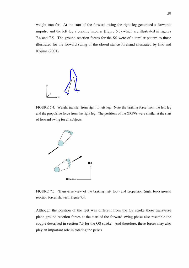
59

weight transfer. At the start of the forward swing the right leg generated a forwards

impulse and the left leg a braking impulse (figure 6.3) which are illustrated in figures

7.4 and 7.5. The ground reaction forces for the SS were of a similar pattern to those

illustrated for the forward swing of the closed stance forehand illustrated by Iino and

Kojima (2001).

x

y

Z

FIGURE 7.4. Weight transfer from right to left leg. Note the braking force from the left leg

and the propulsive force from the right leg. The positions of the GRFVs were similar at the start

of forward swing for all subjects.

Baseline

Net

FIGURE 7.5. Transverse view of the braking (left foot) and propulsion (right foot) ground

reaction forces shown in figure 7.4.

Although the position of the feet was different from the OS stroke these transverse

plane ground reaction forces at the start of the forward swing phase also resemble the

couple described in section 7.3 for the OS stroke. And therefore, these forces may also

play an important role in rotating the pelvis.

60

At the start of the forward swing the GRFVs were anterior and medial to the right knee

and posterior for the left knee (figure 7.4). This helps explain why the main right knee

moments were flexion and abduction while the main left knee moments were extension

for all subjects at the start of the forward swing (figure 6.7).

During the forward swing (approximately -0.2 to 0 seconds), the left knee distal and

lateral forces and left knee abduction and external rotation moments all started to

increase. During the same period, the right knee forces all decreased as the weight had

been transferred to the left leg.

After ball impact and during the follow-through (0 to 0.3 seconds) virtually all the

weight was over the left leg and so the right knee forces were almost zero (figure 6.7).

Since virtually all the weight is over the left leg, the joints in left leg have to endure the

forces and moments necessary to dissipate the rotation energy of the pelvis and upper

body. This caused the distal and lateral forces, and abduction and external rotation

moments to reach their peak (figures 6.7 and 6.8c and tables 6.6 and 6.7). The left knee

abduction moment could be explained by the GRFV being medial to the left knee

(figure 7.6).

Z

y

x

FIGURE 7.6. 0.1s after impact. The GRFV is medial to the left knee, hence the abduction

moment. At this stage of the follow-through, the left knee abduction and external rotation

moments reach their peak. Note also that there is virtually no weight on the right leg.

61

7.5 Suggestion for the role of the lower extremities in generating

pelvic rotation

Iino and Kojima (2001) have stated that the role of the legs in the forehand is to

generate pelvic rotation. The OS and SS strokes appear to use the lower body in

different ways to generate this pelvic motion.

In the OS stroke; the greatest vertical ground reaction force (FZ), ground reaction torque

(TZ), distal, lateral and anterior forces, abduction and external rotation moments were

found in the right leg during the forward swing phase. Therefore, in the OS stoke, the

right leg seems to play the dominant role in aiding pelvic rotation by first flexing and

then forcefully extending whilst pushing laterally and externally rotating. The high

extension moments found in the left knee which contribute to the posterior ground

reaction forces, suggest the left leg also plays a role in assisting pelvic rotation before

impact.

Whereas, in the SS stroke; higher levels of ground reaction torque (TZ), anterior forces,

extension, abduction and external rotation moments were found in the left leg during the

forward swing phase. Therefore, the SS seems to use the stepping action to help

generate pelvic rotation. As the player steps forward he is generating the linear

momentum described in coaching texts such as (Groppel 1992, 77), but as the left foot

hits the ground, the left leg experiences a breaking impulse that is unlikely to be

directed through the CoM of the player. This is similar (although of lesser magnitude)

to the breaking impulses seen in the planting of the front leg in the delivery stride of the

javelin throw (Bartonietz 2000, 420; Bartlett 2007, 196). This combined with the

propulsive force from the right leg (figure 7.4) probably helps to convert the linear

motion into angular motion of the pelvis.

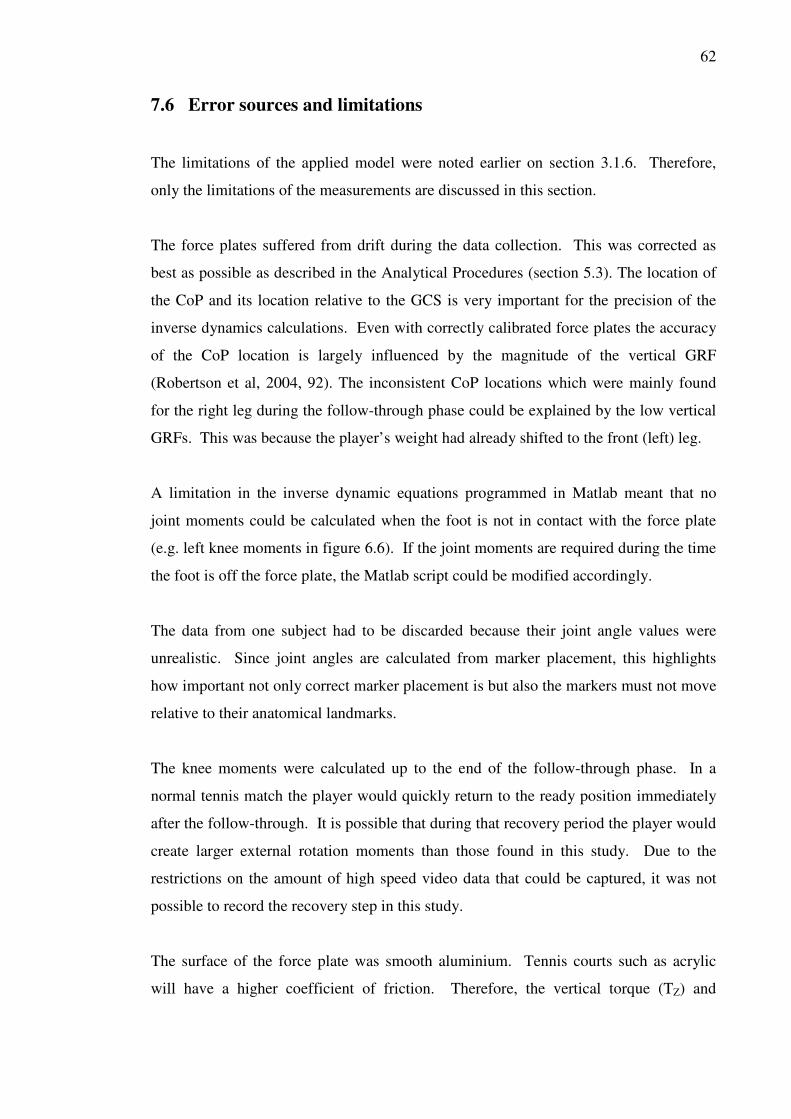
62

7.6 Error sources and limitations

The limitations of the applied model were noted earlier on section 3.1.6. Therefore,

only the limitations of the measurements are discussed in this section.

The force plates suffered from drift during the data collection. This was corrected as

best as possible as described in the Analytical Procedures (section 5.3). The location of

the CoP and its location relative to the GCS is very important for the precision of the

inverse dynamics calculations. Even with correctly calibrated force plates the accuracy

of the CoP location is largely influenced by the magnitude of the vertical GRF

(Robertson et al, 2004, 92). The inconsistent CoP locations which were mainly found

for the right leg during the follow-through phase could be explained by the low vertical

GRFs. This was because the player’s weight had already shifted to the front (left) leg.

A limitation in the inverse dynamic equations programmed in Matlab meant that no

joint moments could be calculated when the foot is not in contact with the force plate

(e.g. left knee moments in figure 6.6). If the joint moments are required during the time

the foot is off the force plate, the Matlab script could be modified accordingly.

The data from one subject had to be discarded because their joint angle values were

unrealistic. Since joint angles are calculated from marker placement, this highlights

how important not only correct marker placement is but also the markers must not move

relative to their anatomical landmarks.

The knee moments were calculated up to the end of the follow-through phase. In a

normal tennis match the player would quickly return to the ready position immediately

after the follow-through. It is possible that during that recovery period the player would

create larger external rotation moments than those found in this study. Due to the

restrictions on the amount of high speed video data that could be captured, it was not

possible to record the recovery step in this study.

The surface of the force plate was smooth aluminium. Tennis courts such as acrylic

will have a higher coefficient of friction. Therefore, the vertical torque (TZ) and

63

subsequent knee external rotation moments calculated from this study may have been

larger if a representative surface could have been fixed onto the top of the force plate.

An additional limitation of this study was the size of the force plates and the size of the

area that the data could be reliable captured. This did not allow a great deal of

movement prior to hitting the ball. During match conditions the players are more likely

to be running prior to stabilising themselves for the forward swing.

7.7 Coaching implications

On the basis of this study one cannot advocate one type of forehand over another.

Although, coaches who train players with knee problems or those recovering from knee

injury or knee surgery should be aware that the OS forehand loads the right knee joint

before impact while the SS forehand loads the left knee after contact. Therefore, a

player recovering from right knee injury may want to try to utilise more linear motion in

their forehand. Similarly, a player recovering from a left knee injury may want to use a

more open stance.

7.8 Suggestions for further study

The role of the lower body in rotating the pelvis in the OS forehand could be examined

in greater detail. This has been performed on the CS forehand (Iino & Kojima 2001)

and backhand (Akutagawa & Kojima, 2005), but not on the OS forehand. The results of

this work suggest that the right leg may make a greater contribution to pelvic torque in

the OS forehand compared to the levels reported by Iino & Kojima (2001) for the CS

forehand.

Electromyographic techniques could be incorporated into an inverse dynamic study of

the lower body. By incorporating the electromyography (EMG) data, an understanding

of the muscle activation patterns and timing, and their role in generating the resultant

joint moments and forces could be obtained.

In the OS stroke the player can transfer their weight onto the leading foot before or after

64

contact. In the SS stroke the weight transfer occurs before contact. So, it is possible

that if the forward weight transfer occurs before contact in the OS stroke, the TZ forces

and external rotation moments in the right leg may be lower. Therefore, a study could

be performed to investigate the differences between the loading of the lower body in the

OS stroke for weight transfer before contact and weight transfer after contact.

The linear and angular momentum, and total body energy of the OS and SS forehands

could be calculated. For example, if the total body mechanical energy can be calculated

it could be used to show how much energy the supporting leg has to dissipate in the

follow-through. Angular momentum has been calculated for the tennis backhand

(Wang et al. 2010) and serve (Bahamonde, 2000), while power analysis has been used

to analyse the golf swing (Nesbit, 2005), but to date no data is available for the tennis

forehand. This is despite the fact that the conversion of linear to angular momentum is

frequently described in coaching texts (Papas, 2008).

A more complex model of the knee joint could be used to estimate tendon, ligament and

joint contact loads such as that used by Shelburne et al. (2005) or an EMG driven

neuromuscular model used by Lloyd et al. (2005). Commercially available computer

simulators such as LifeModeler®

KneeSim (LifeModeler Inc. San Clemente, California,

USA) could also be used. This could be combined with further investigations to

highlight the potential for the tennis forehand to cause an overuse injury in the knee.

There are slight differences in the anatomy of the knee joint in men and women

(Palastanga, 2002), and the loading of the knee joint has been shown to differ between

men and women in other movements (Pollard et al, 2007). Therefore, a study to

investigate the sex differences in the knee kinetics of the tennis strokes could be

beneficial.

65

8 CONCLUSIONS

In this study, both OS and SS forehands displayed similar levels of pelvic angular

velocity, swing times and racket head speeds. Therefore, although the two types of shot

involved contrasting movement patterns of the lower body, the effect on the ball was the

same and so both shots used the lower body in different ways to produce the same end

result.

Although the peak loads are similar, the OS forehand creates greater loads on the right

knee joint before impact while the SS forehand creates greater loads on the left knee

during the follow-through. This loading occurs with the knee in a more flexed position

in the OS forehand. The extension, abduction and torsional forces generated in the right

leg assist in the generation of the angular motion of the pelvis in the OS forehand

whereas, the checking action of the left leg assists in the conversion of linear to angular

motion in the SS forehand.

66

9 REFERENCES

Akutagawa, S. & Kojima. T. 2005. Trunk rotation torques through the hip joints during

the one- and two-handed backhand tennis strokes. Journal of Sports Sciences

23 (8), 781-793.

Allard, P. 1997. Able-bodied gait in men and women . In: Allard, P., Cappozzo,

A.,Lundberg, A & Vaughan, C. (eds.) Three-dimensional analysis of human

locomotion. Wiley, W. Sussex, England, 307-334.

Andrews, J., G. 1995. Euler’s and Lagrange’s equations for linked rigid–body models of

three-dimensional human motion. In Allard, P., S. Ian, A., F., & Blanchi, JP.

(eds.) Three dimensional analysis of human movement. Human Kinetics

Publishers Inc. 153-175.

Ariel, G. Calculating Euler angles in 3D lower extremity kinematics and kinetics.

http://www.sportsci.com/adi2001/adi/services/support/manuals/apas/3Dkin/doc5

.asp. 10.11.2008.

Bahamonde, R. 2000. Changes in angular momentum during the tennis serve. Journal of

Sports Sciences 18(8), 579-592.

Bahamonde, R. & Knudson, D. 2003. Kinetics of the upper extremity in the open and

square stance tennis forehand. Journal of Science and Medicine in Sport 6 (1):

88-101.

Bartlett, R. 2007. Introduction to sports biomechanics (2nd

ed.). Routledge.

Bartonietz, K. 2000. Javelin throwing: an approach to performance development. In:

Zatsiorsky V. (ed.) Biomechanics in sport. Blackwell Science. Cambridge

University Press, 401-434.

Beer, F. & Johnston, R. 2004. Vector Mechanics for Engineers Statics & Dynamics

(7th

ed ). McGraw-Hill.

Besier, T., Lloyd, D., Cochrane, J. & Ackland, T. 2001. External loading of the knee

joint during running and cutting manoeuvres. Medicine and Science in Sport and

Exercise 33, 1168-1175.

Bollettieri, N. 2001. Bollettieri's Tennis Handbook. Human Kinetics Publishers Inc.

Crespo, M. & Higueras, J. 2001. Forehands. In: Roetert, P. & Groppel, J. (eds.). World

Class Tennis Technique. Human Kinetics Publishers Inc. 149-151.

Crespo, M. & Reid, M. 2003. Biomechanics and teaching methodology. In: Elliott B.,

67

Reid M., & Crespo M., (Eds.) Biomechanics of advanced tennis.

The International Tennis Federation, ITF Ltd., 15-29.

Ellenbecker, T. 2006. USTA High Performance Coaching Newsletter. Vol 8 No.2.

USTA.

Elliott, B., Takahashi, K. & Noffal, G. 1997. The influence of grip position on upper

Limb contributions to racket-head speed in the tennis forehand. Journal of

Applied Biomechanics 13 (2), 182-196.

Elliott, B. C. 2002. Biomechanics of tennis. In: Renström P. A. F. H. (ed.) Tennis.

IOC Medical Sub-Commission on Publications in the Sport Sciences. Blackwell

Science, Oxford, UK, 1-28.

Elliott, B. C. 2003. The development of racket speed. . In: Elliott B., Reid M., &

Crespo M., (Eds.) Biomechanics of advanced tennis. The International Tennis

Federation, ITF Ltd., 111-125.

Elliott, B. C. 2006. Biomechanics and tennis. British Journal of Sports Medicine

40, 392-396.

Enoka, R. M. 2008. Neuromechanics of Human Movement. 4th

edn. Human Kinetics

Publishers Inc.

Finni, T., Komi, P.V. & Lukkariniemi, J. 1998. Achilles tendon force during walking:

measurements with the optic fibre technique. European Journal of Applied

Physiology 77, 289-291.

Gatt, C.J., Pavol, M. J., Parker, R. D., & Grabiner, M, D. 1999. A kinetic analysis of the

knees during a golf swing. In: Farrally, M. & Cochran, A. (eds.) Science and

Golf III. Human Kinetics Publishers Inc.

van Gheluwe, B. & Hebbelinck, M. 1986. Muscle actions and ground reaction forces in

tennis. International Journal of Sport Biomechanics 2, 88-99.

Goldstein, H. 1980. Classical Mechanics, 2nd

edn. Addison-Wesley.

Greenwood, D. T. 2006. Advanced Dynamics. Cambridge University Press.

Gregory, R. J., Komi P.V., Browning, R., C. & Jarvinen, M. 1991. A comparison of the

triceps surae and residual muscle moments at the ankle during cycling. Journal

of Biomechanics 24, 287-297.

Grimshaw, P., Lees, A., Fowler, N. & Burden, A. 2006. Sport & Exercise

Biomechanics. Taylor & Francis.

Groppel, J. 1992. High Tech Tennis, 2nd

edn. Leisure Press, Champaign, IL., USA.

Hamil, J. & Knutzen, K. 2003. Biomechanical Basis of Human Movement (2nd ed)

68

Lippincott Williams & Wilkins.

Huang, C-F. & Lin, C-L. 2011. The characteristics of lower limb moments in baseball

pitching. Portuguese Journal of Sport Sciences 11 (Suppl. 2), 89-92.

Iino, Y. & Kojima, T. 2001. Torque acting on the pelvis about its superior-inferior axis

through the hip joints during a tennis forehand stroke. Journal of Human

Movement Studies 40, 269-290.

Iino, Y. & Kojima, T. 2003. Role of knee flexion and extension for rotating the trunk in

a tennis forehand stroke. Journal of Human Movement Studies 45, 133-152.

ISB Kistler. http://isbweb.org/software/movanal/vaughan/kistler.pdf 10.2.08.

ITF, 2007. ITF. http://www.itftennis.com/abouttheitf/nationalassociations/index.asp.

23.04.07

Jose, J. V. & Saletan, E. J. 1998. Classical Dynamics: A Contemporary Approach.

Cambridge University Press.

Kerrigan, D. C., Franz, J. R., Keenan, G. S., Dicharry, J., Ugo Della Croce, & Wilder,

R. P., 2009. The effect of running shoes on lower extremity joint torques.

American Academy of Physical Medicine and Rehabilitation 1, 1058-1063.

Kibbler, W. Ben. & van der Meer, D. 2001. Mastering the kinetic chain In: Roetert, P.

& Groppel, J. (eds.). World Class Tennis Technique. Human Kinetics Publishers

Inc. 99-113.

Kirtley, C. 2006. Clinical Gait Analysis. Elsevier Churchill Livingstone.

Knudson, D. 2006. Biomechanical Principles of Tennis Technique. Racquet Tech

Publishing, California, USA.

Knudson D. & Blackwell, J. 2000. Trunk muscle activation in open stance and square

stance tennis forehands. International Journal of Sports Medicine 21, 321-324.

Knudson D. & Elliott B. 2004. Biomechanics of tennis strokes. In: Hung G. & Pallis J.

(Eds.) Biomedical engineering principles in sports. Kluwer Academic/Plenum

Publishers, New York, 153-171.

Komi P.V., Belli, A., Huttunen, R., Bonnefoy, A., Geysant, A. & Lacour, J.R. 1996.

Optic fibre as a transducer of tendomuscular forces. European Journal of

Applied Physiology and Occupational Physiology 72, 278-280.

Komi, P.V. & Nicol, C. 2000. Stretch-shortening cycle of muscle function. In:

Zatsiorsky V. (ed.) Biomechanics in sport. Blackwell Science. Cambridge

University Press, 87-102.

Landlinger, J., Lindinger, S., Stöggl, T., Wagner, H. & Müller, E. 2010. Key factors and

69

timing patterns in the tennis forehand of different skill levels. Journal of Sport

Science and Medicine 9, 643-651.

Langevad, B. 2003. Ace Tennis Magazine. Tennis GB Ltd. April 2003, 46-47.

Lees, A. & Lake, M. 2008. Force and Pressure Measurement. In: Payton, C. J. &

Bartlett, R. M. (eds.) Biomechanical Evaluation of Movement in Sport and

Exercise. Routledge, Oxford, England, 53-76.

LifeModeler kneeSIMM,. http://www.lifemodeler.com/products/kneesim/. 10.11.2011.

Livesay, G., Woo, S., Runco, T. & Rudy, T. 1997. Application of robotics technology

to the study of knee kinematics. In: Allard, P., Cappozzo, A., Lundberg, A &

Vaughan, C. (eds.) Three-dimensional analysis of human locomotion. Wiley,

W. Sussex, England, 230-257.

Lloyd, D., G, Buchanan, T., S. & Besier, T., F. 2005. Neuromuscular biomechanical

modelling to understand knee ligament loading. Medicine and Science in Sports

and Exercise, 37(11), 1939-1947.

Lynn, S., & Noffal, G. J. 2010. Frontal plane moments in golf: Effect of target side foot

position at address. Journal of Sport Science and Medicine 9, 275-281.

McGinnis, P. M. 2005. Biomechanics of sport and exercise. Human Kinetics Publishers

Inc.

Marshall, R. N. & Elliott, B., C. 2000. Long-axis rotation: the missing link in proximal

to distal sequencing. Journal of Sport Sciences 18, 247-254.

Miller, D. 1990. Ground reaction forces in distance running. In: Cavanagh, P. R. (ed.)

Biomechanics of Distance Running. Human Kinetics, 203-224.

Nesbit, S.M. & Serrano, M. 2005. Work and power analysis of the golf swing. Journal

of Sports Sciences and Medicine 4, 520-533.

Nigg, B. M. 2007. Force system analysis. In: Nigg, B.M & Herzog, W (eds.)

Biomechanics of the Musculo-skeletal System. (3rd

ed.). Wiley, W. Sussex,

England. 523-534.

Papas, M. 2008. Modern tennis not.

http://www.revolutionarytennis.com/moderntennisnot3_4.html. 07.04.2012.

Perry, A., C., Wang, X., Feldman, B.,B., Ruth, T. & Signorile, J. 2004. Can laboratory-

based tennis profiles predict field tests of tennis performance? Journal of

Strength and Conditioning Research 18, 136-143.

Pluim, B., Miller, S., Dines, D., Renström, P., Windler, G., Norris, B., Stroia, K.,

Donaldson, A. & Martin, K. 2007. Sport science and medicine in tennis. British

70

Journal of Sports Medicine. 41, 703-704.

Pollard, C., D., Sigward, S., M. & Powers, C., M. 2007. Gender differences in hip joint

kinematics and kinetics during side-step cutting maneuver. Journal of Sports

Medicine. 17, 38-42.

Reid, M. Chow, J., W. & Crespo, M. 2003. Muscle activity: an indicator for training. In:

Elliott B., Reid M. & Crespo M., (Eds.) Biomechanics of advanced tennis. The

International Tennis Federation, ITF Ltd., 111-125.

Robertson, D., Caldwell, G., Hamill, J., Kamen, G. & Whittlesey, S. 2004. Research

Methods in Biomechanics. Human Kinetics.

Roetert, E., Kovacs, M., Knudson, D. & Groppel, J. 2009. Biomechanics of the tennis

groundstrokes: Implications for Strength Training. Journal of Strength and

Conditioning 31, 4, 41-49.

Saviano, N. 1997. How to hit today’s big forehand. Tennis Magazine. Miller

Publishing. November, 28-34.

Seliktar, R., & Bo L. 1995. The theory of kinetic analysis in human gait. In: Craik, R.,

L. & Oatis, A. (Eds.) Gait Anlysis: Theory and Application. Mosby-Year Book

Inc.

Shelbourne, K., Torry, M. & Pandy, M. 2005. Muscle, ligament and joint-contact forces

at the knee during walking. Medicine & Science in Sports & Exercise 47, 1948-

1956.

Shen, W. Euler angle calculation in Vaughan book.http://biomchl.isbweb.org/threads

/9337-Euler-angle-calculation-in-Vaughan-s-book. 21.11.2012.

Siegler, S & Liu, W. 1997. Inverse dynamics in human locomotion. In: Allard, P.,

Cappozzo,A., Lundberg, A & Vaughan, C. (eds.) 1997. Three-dimensional

analysis of human locomotion. Wiley, W. Sussex, England.

Simonsen, E.B., Dyhre-Poulsen, P., Voigt, M., Aagaard, P. & Fallentin, N. 1997.

Mechanisms contributing to different joint momentsobserved during human

walking. Scandinavian Journal of Medicine and Science in Sports 7 (1) 1-13.

USTA 2005. http://www.usta.com/news/fullstory.sps?inewsid=280183. 30.04.2007.

Van Gheluwe, B. & Hebbelinck, M. 1986. Muscle actions and ground reaction forces in

tennis. International Journal of Sport Biomechanics 2, 88-99.

Vaughan, C. L., Davis, B.L. & O’Connor, J.C. 1992. Dynamics of human gait. Cape

Town. South Africa, Kiboho Publishers.

Vaughan, C. L., Davis, B.L. & O’Connor, J.C. 1999. Dynamics of human gait. (2nd

71

ed.). Cape Town. South Africa, Kiboho Publishers.

Wang, L.H., Lin, H.,T. Lo, K.,C. Hsieh, Y.,C & Su, F.,C. 2010. Comparison of

Segmental linear and angular momentum transfers in two-handed backhand

stroke stances for different skill level tennis players. Journal of Science and

Medicine in Sport 13, 452-459.

Whiting, W. & Zernicke, R. 1998. Biomechanics of musculoskeletal injury. Human

Kinetics Publishers Inc.

Wikipedia. http://en.wikipedia.org/wiki/Euler_angles. 20.09.11.

Winter, D. 2005. Biomechanics and motor control of human movement (3rd

ed.). Wiley

Inc.

Worsfold, P., Smith, N., A. & Dyson, R., J. 2008. Low handicap golfers generate more

torque at the shoe-natural grass interface when using a driver. Journal of Sports

Science and Medicine 7, 408-414.

Yamaguchi G., T. 2004. Dynamic modeling of musculoskeletal motion. Kluwer

Academic Publishers.

Zatsiorsky, V. 1998. Kinematics of human motion. Human Kinetics Publishers Inc.

Zatsiorsky, V. 2002. Kinetics of human motion. Human Kinetics Publishers Inc.

72

10 APPENDIX

10.1 Definition of the Euler angles using the Z, line of nodes, z

rotation sequence

To derive the equations for the angular velocity of the segment the in terms of the LCS

(equation 14), three successive rotations of the LCS will be described. The rotations

start with the axes of the LCS coinciding with the axes of the GCS and ends with the

LCS back in its original orientation. The first rotation takes place about the global Z

axis, the second about the line of nodes and the third about the z axis of the segment.

The complete sequence is shown in figure 10.1. The line of nodes is defined as the

intersection of the x’segment, y

’segment and the X, Y planes (figure 10.1b). This can be

expressed mathematically as the cross product of the Z and zsegment axes (Goldstein

1980, 145; Jose & Saletan 1998, 526; Vaughan et al 1999, 98).

The sequence commences by rotating the LCS, by an angle φ counter-clockwise about

the global Z axis (figure 10.1a), the resultant coordinate system is labelled x’’

segment,

y’’

segment, z’’

segment. Next, the x’’

segment, y’’

segment, z’’

segment axes are rotated counter-

clockwise about the line of nodes by an angle θ to produce another set of intermediate

axes x’segment, y

’segment, z

’segment (figure 10.1b). Finally, the x

’segment, y

’segment, z

’segment

axes are rotated counter-clockwise about the z’segment by an angle ψ to produce the

desired xsegment, ysegment, zsegment axes (figure 10.1c). This is now the original orientation

of the LCS.

These three rotations can be described numerically using transformation matrices. The

three matrices are:

A =

100

0 cossin -

0sincos

φφ

φφ

(23)

73

θ

φ

ψ.

.

.

FIGURE 10.1. Definition of the 3 Euler angles (φsegment , θsegment , ψsegment). The rotations take

place in the following order: (a) φsegment about the Z axis; (b) θsegment about the line of nodes; and

(c) ψsegment about the z segment axis (Vaughan et al. 1999, 98).

74

B =

θθ

θθ

cossin0

sincos0

001

-

(24)

C =

100

0cossin

0sincos

ψψ

ψψ

- (25)

where A, B and C represent the rotation matrices for the first, second and third rotation

respectively.

The complete sequence of rotation is described by taking the product of these 3 matrices

D = CBA (26)

which gives the following transformation matrix:

D =

+

+−

θφθφθ

θψψθφψψφθφψ

θψψφθφψψφθφψ

cossin sin -sin sin

sin coscos cos cossin sin-cossin cos-cos sin-

sin sinsincoscossincossinsincoscoscos

φ (27)

10.2 Angular velocity of the segment

If the vector ω represents the resultant instantaneous angular velocity of the LCS, then

ω can be described as the sum of the angular velocity vectors pointing in the direction

of the axes of rotation:

ω = ωφ + ωθ + ωψ (28)

where ωφ, ωθ, and ωψ represent the components of the angular velocity vector ω about

the global Z axis, the line of nodes and the zsegment axes respectively.

75

However, for calculating the net moment of the segment, the components of ω along the

segment axes (xsegment, ysegment, zsegment) need to be defined. The time derivatives of the

Euler angles cannot be used directly, as that gives the components ω about 3 axes of

rotation (as shown in figure 10.1c and described by equation (26)). Fortunately, the

matrices in equations (22 to 25) can be used to find the components of the angular

velocity vectors along each one of the axes of the LCS. This is achieved by finding the

respective xsegment, ysegment, zsegment components of ωφ, ωθ, and ωψ and then simply

adding them together (Goldstein 1980, 176).

Since ωφ lies along the global Z axis, the complete rotation sequence (matrix D) needs

to be used. This gives:

D

•

φ

0

0

=

cos

cos sin

sin sin

θφ

ψθφ

ψθφ

•

•

•

(29)

where (ωφ) xsegment = ψθφ sin sin •

, (ωφ) ysegment = ψθφ cos sin •

, (ωφ) zsegment = cos θφ•

ωθ lies along the line of nodes which coincides with the x’’

segment axis. The components

of ωθ are obtained by applying only the final transformation i.e. matrix C.

C

•

0

0

θ

=

0

sin

cos

ψθ

ψθ•

•

− (30)

where (ωθ) xsegment = ψθ cos •

, (ωθ) ysegment = ψθ sin -•

, (ωθ) zsegment = 0

No transformation is necessary for the components of ωψ, becuase ωψ lies along the

zsegment axis. This means:

(ωψ) xsegment = 0, (ωψ) ysegment = 0, (ωψ) zsegment = •

ψ (31)

76

Adding their respective components gives equation (14), the angular velocity about the

local axes of the segment (Goldstein 1980, 145; Jose & Saletan 1998, 526; Vaughan et

al 1999, 98):

+= ψθφω sinsin.&

xsegment ψθ cos&

ψθψθφω sincossin.&& −=ysegment (14)

ψθφω && += cos.zsegment

10.3 Angular acceleration of the segment

Since acceleration is defined as the second time derivative of displacement, the segment

angular accelerations are calculated by taking the derivative of equation (14) which

gives the following (Vaughan et al 1999, 97):

ψψθψθψθψφψθθφψθφω sincoscossinsincossinsin.&&&&&&&&&&& −+++=xsegment

ψψθψθψθψφψθθφψθφω cossinsinsincoscoscossin.&&&&&&&&&&& −−−+=ysegment (15)

ψθθφθφω &&&&&&& +−= sincos.zsegment

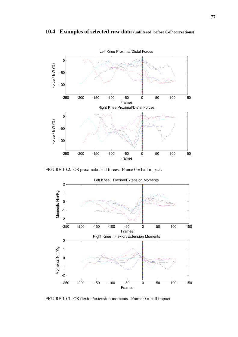
77

10.4 Examples of selected raw data (unfiltered, before CoP corrections)

-250 -200 -150 -100 -50 0 50 100 150

-100

-50

0

Left Knee Proximal/Distal Forces

Frames

Forc

e /

BW

(%

)

-250 -200 -150 -100 -50 0 50 100 150

-100

-50

0

Right Knee Proximal/Distal Forces

Frames

Forc

e /

BW

(%

)

FIGURE 10.2. OS proximal/distal forces. Frame 0 = ball impact.

-250 -200 -150 -100 -50 0 50 100 150

-2

-1

0

1

2Left Knee Flexion/Extension Moments

Frames

Mom

ents

Nm

/Kg

-250 -200 -150 -100 -50 0 50 100 150

-2

-1

0

1

2Right Knee Flexion/Extension Moments

Frames

Mom

ents

Nm

/Kg

FIGURE 10.3. OS flexion/extension moments. Frame 0 = ball impact.

78

-250 -200 -150 -100 -50 0 50 100 150-0.5

0

0.5

Left Knee Internal/External Moments

Frames

Mom

ents

Nm

/Kg

-250 -200 -150 -100 -50 0 50 100 150-0.5

0

0.5

Right Knee Internal/External Moments

Frames

Mom

ents

Nm

/Kg

FIGURE 10.4. OS internal/external rotation moments. Frame 0 = ball impact.

-250 -200 -150 -100 -50 0 50 100 150

-1

0

1

Left Knee Abduction/Adduction Moments

Frames

Mom

ents

Nm

/Kg

-250 -200 -150 -100 -50 0 50 100 150

-1

0

1

Right Knee Abduction/Adduction Moments

Frames

Mom

ents

Nm

/Kg

FIGURE 10.5. OS abduction/adduction moments. Frame 0 = ball impact.

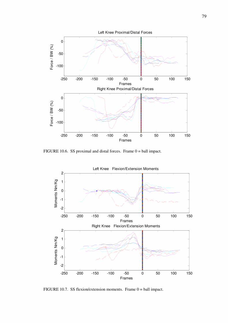
79

-250 -200 -150 -100 -50 0 50 100 150

-100

-50

0

Left Knee Proximal/Distal Forces

Frames

Forc

e /

BW

(%

)

-250 -200 -150 -100 -50 0 50 100 150

-100

-50

0

Right Knee Proximal/Distal Forces

Frames

Forc

e /

BW

(%

)

FIGURE 10.6. SS proximal and distal forces. Frame 0 = ball impact.

-250 -200 -150 -100 -50 0 50 100 150

-2

-1

0

1

2Left Knee Flexion/Extension Moments

Frames

Mom

ents

Nm

/Kg

-250 -200 -150 -100 -50 0 50 100 150

-2

-1

0

1

2Right Knee Flexion/Extension Moments

Frames

Mom

ents

Nm

/Kg

FIGURE 10.7. SS flexion/extension moments. Frame 0 = ball impact.

80

-250 -200 -150 -100 -50 0 50 100 150-0.5

0

0.5

Left Knee Internal External Moments

Frames

Mom

ents

Nm

/Kg

-250 -200 -150 -100 -50 0 50 100 150-0.5

0

0.5

Right Knee

Frames

Mom

ents

Nm

/Kg

FIGURE 10.8. SS internal/external rotation moments. Frame 0 = ball impact

-250 -200 -150 -100 -50 0 50 100 150

-2

-1

0

1

2Left Knee Abduction/Adduction Moments

Frames

Mom

ents

Nm

/Kg

-250 -200 -150 -100 -50 0 50 100 150

-2

-1

0

1

2Right Knee Abduction/Adduction Moments

Frames

Mom

ents

Nm

/Kg

FIGURE 10.9. Square stance abduction/adduction moments. Frame 0 = ball impact.