SEMI-ANNUAL REPORT/

DEVELOPMENT OF A COMPUTERIZED ANALYSISFOR

SOLID PROPELLLANT COMBUSTION INSTABILITY WITH TURBULENCE

NAG8-627

by

T. J. Chung and 0. Y. Park

Department of Mechanical EngineeringThe University of Alabama in Huntsville

prepared for

NASA/MSFC

(KASA-CB-162351) BEVILOPHEtfT OF A. N88-2S497COMPUTERIZED AD111SIS FOR SCUD EEOPELLAtJlCCJ5BOS1ICB IJSS14£JLIT? SITE 3DEED1EKCESeaiajinual Report (A labama C-n iv . ) U9 p Unclas

CSCI 21B G3/25 01U8510

May, 1988

https://ntrs.nasa.gov/search.jsp?R=19880016113 2018-07-06T15:25:53+00:00Z

ABSTRACT

A multi-dimensional numerical model has been'developed for

the unsteady state osci]latory combustion of solid propellants

subject to acoustic pressure disturbances. Including the gas

phase unsteady effects, the assumption of uniform pressure across

the flame zone, which has been conventionally used, is relaxed

such that a higher frequency response in the long flame of a

double-base propel1ant can be calculated. The formulation is

based on a premixed, laminar flame with a one-step overall

chemical reaction and the Arrhenius law of decomposition with not

condensed phase reaction. In a given geometry, the Galerkin

finite element solution shows the strong resonance and damping

effect at the lower frequencies, similar to the result of Denison

and Baum. Extended studies deal with the higher frequency region

where the pressure varies in the flame thickness. The nonlinear

system behavior is investigated by carrying out the second order

expansion in wave amplitude when the acoustic pressure

oscillations are finite in amplitude. Offset in the burning rate

shows a negative sign in the whole frequency region considered,

and it verifies the experimental results of Price. Finally, the

velocity coupling in the two-dimensional model is discussed.

NOMENCLATURE

a speed of sound

B frequency factor for gas phase reaction

Cp specific heat at constant pressure for gas

Cs specific heat of solid

E gas phase activation energy

E8 surface activation energy

F eigenvector

G source term in numerical formulation

h heat of combustion per unit mass

H heat of reaction

I order"of perturbation

k thermal conductivity

jj characteristic flame length

L latent heat of vaporization

m mass flux

Mb Mach number

n order of chemical reaction

P pressure

Pr Prandtl number

r burning rate

R gas constant

Rc dimensionless distance from surface in Eq. (22)

t time

T temperature

u axial gas velocity

Uj velocity vector

uc core velocity in Eq. (22)

v normal gas velocity

w reaction rate

x axial distance parallel to the surface

X solution vector

y normal distance from the surface

Y mass fraction of fuel species

z oxidizer-fuel ratio

a thermal diffusivity

fl ratio of solid to gas density

a temperature exponent in Eq. (7)

•y specific heat ratio

e perturbation parameter

{ = ks*Cp*/k*Cs*

\ eigenvalue

\y Lagrange multiplier

p density

u frequency

Subscripts, and Superscripts

* dimensional quantity

steady-state mean value

A spatial variable

(i) ith order perturbation coefficient

+ gas side of interface

solid side of interface

c propellant cold side

D time-dependent variable

i,j vector quantity

I time-independent variable

0 mean value at flame edge

s solid phase

a, 6 finite element global node number

t complex conjugate

1. INTRODUCTION

An accurate analysis of combustion instability resulting

from the oscillatory burning of solid propellants has long been

of major concern. Such an analysis is characterized by the

acoustic admittance or response function, a proper measure of

instability. However, experimental measurements of the

coefficients are difficult; thus, it is desirable that analytical

or numerical calculations be implemented whenever possible.

Most of the past investigations on combustion instability

have been centered around a one-dimensional quasi-steady analysis

limited to pressure coupling [1-19]. The representative studies

were accomplished by Hart and McClure [2], Denison and Baum [4],

and Culick [12-14]. Culick's review article [12] on homogeneous

propellants summarizes the state-of-the-art up to the late 1960's

and discusses the limitations of the analyses. Recently, several

works concerning unsteady state problems have been attempted [20-

27]. T'ien [21] introduces improved gas dynamics in order to

recover the quasi-steady limitations by considering both gas and

solid phases in an unsteady manner. However, the pressure is

still assumed to be constant and a function of time only, which

has generally been used. Consequently, as indicated, in the case

of the long flame of a double-base propellant, application of the

model is limited to lower frequencies.

Flandro [23,24] presents the first attempt to examine the

response functions under the effect of incident acoustic waves in

a two-dimensional analysis. A detailed formulation is extended

to the second order perturbation system in terms of the Prandtl

number and the Mach number. The effects of viscosity and heat

transfer in the gas phase are included. The numerical results

for the first order system appear to be comparable to those of

T'ien [21]; however, the results of the second order response

function are not clear. Moreover, details of matching conditions

are not given. The requirements for a more realistic model of

combustion instability have lead to quite a number of rigorous

studies. One recent work deals with the heterogeneous

propellants summarized in Cohen's review paper [30-33].

The major discussions of the acoustic admittance or response

function in the literature are concerned with pressure coupling

usually applicable in the linear stability. Computations of the

response function for velocity coupling are important in a

nonlinear process; however, they remain in a state of infancy,

although some initial attempts toward this subject have been made

[34-38]. Observations indicate that combustion oscillations are

time-dependent and often nonlinear, as influenced by turbulent

flow fields which may lead to erosive burning and unstable

oscillations. Since the complicated physical phenomena cannot be

described analytically, some approximations and simplifications

are still introduced to the theoretical formulations in the

numerical analyses. Recently, Chung and Kim [26] introduced the

effect of radiative heat transfer on the combustion instability

in solid rocket motors based on the research of Chung and Kim

[27]. Further research has been reported concerning the

calculation of response functions in multi-dimensional combustion

phenomena [28]. The finite element method is introduced and

complicated boundary conditions are handled easily by means of

Lagrange multipliers [29].

On the other hand, much experimental effort has been devoted

to understanding the oscillatory combustion mechanism using the f

T-burner and L*-burner [39-42]. Extensive experiments may be

found in the recent series of papers conducted by Levine and Baum

[43,44]. Also, in the work of Caveny et al. [45], the

oscillatory velocities in the solid propellant flames subject to

pressure coupling are measured directly using the laser Doppler

velocimetry instrumentation.

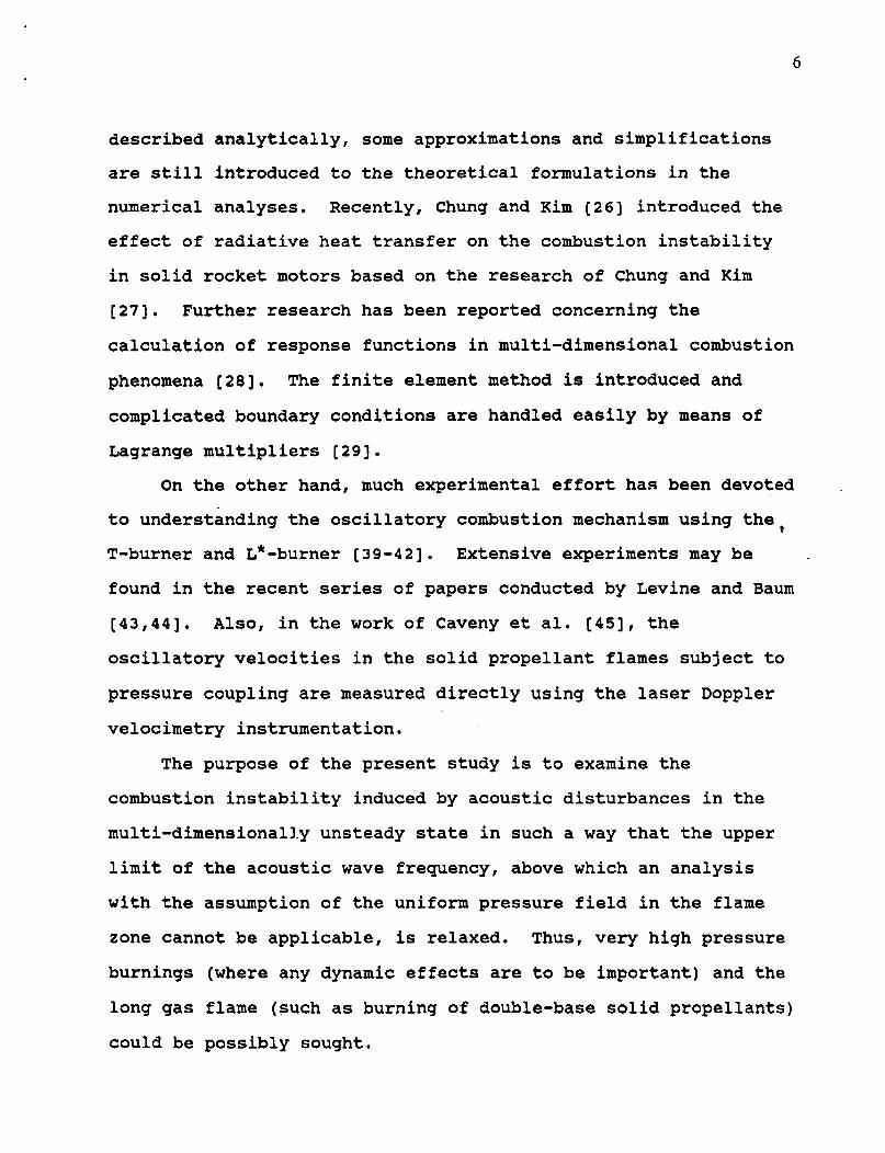
The purpose of the present study is to examine the

combustion instability induced by acoustic disturbances in the

multi-dimensionally unsteady state in such a way that the upper

limit of the acoustic wave frequency, above which an analysis

with the assumption of the uniform pressure field in the flame

zone cannot be applicable, is relaxed. Thus, very high pressure

burnings (where any dynamic effects are to be important) and the

long gas flame (such as burning of double-base solid propellants)

could be possibly sought.

For small amplitude oscillations, the nonsteady governing

equations are linearized by means of the first and second order

perturbation expansions and solved numerically using the finite

element method. The theoretical model is still based on a

homogeneous propellant, Lewis number of unity, a second-order,

single-step forward chemical reaction, and vaporization in an

Arrhenius fashion, with no erosive burning.

2. ANALYSIS

For the simplicity of the combustion modeling of solid

propellants, the gaseous flame is assumed to be multi-

dimensional, premixed laminar, and calorically perfect, and a

one-step forward chemical reaction occurs. The combustion of a

solid propellant is approximated by the Arrhenius ].aw. The Lewis

number is given as unity for the explicit relation between

concentration and temperature. Thus, the conservation laws for

the multi-component reactive system in the gas phase are

represented as follows:

Continuity

dp— + (P̂ )̂ o 0 (1)8t

Momentum

3Ui 1 f 1P " + pUi/jUj + ~ P/i " prUi'jj +dt '^b

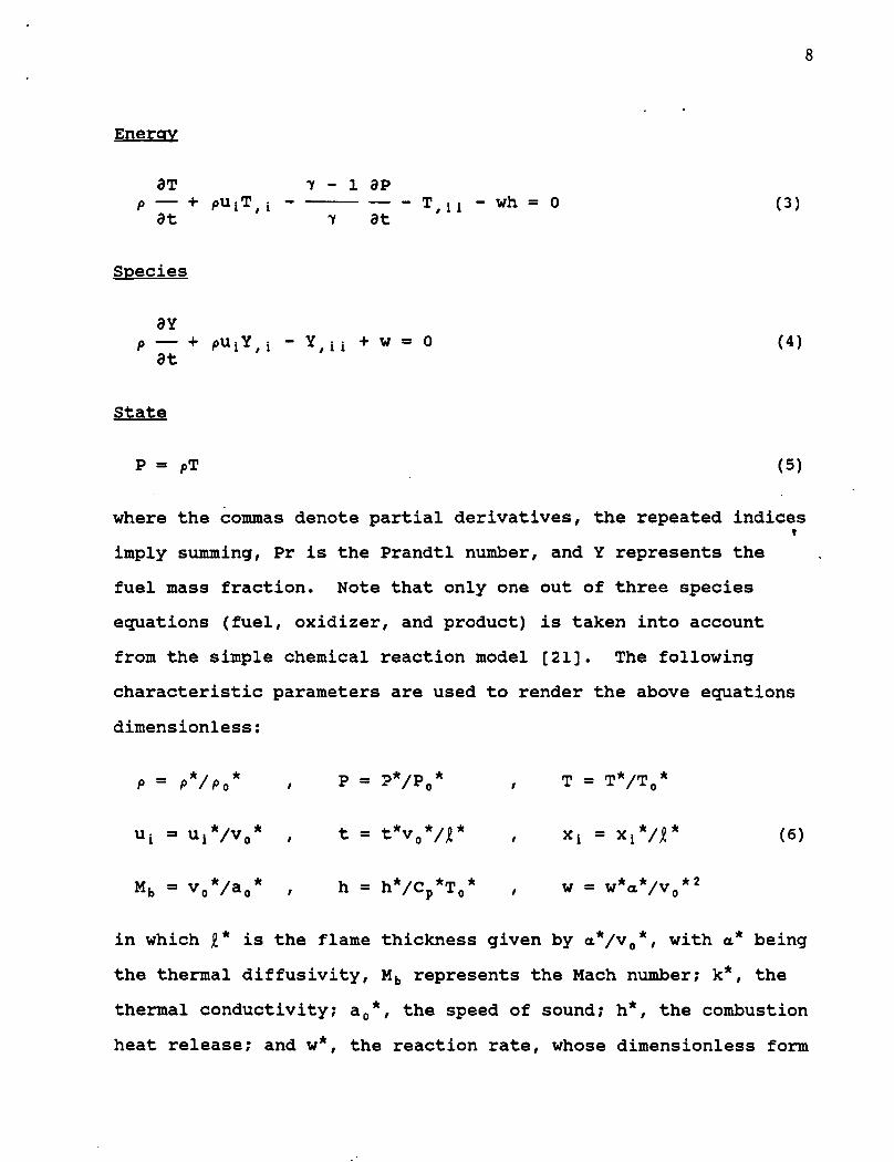
Energy

3T 1 - 1 3Pp — + pUtTfi T/n - wh = 0 (3)a t - / a t

Species

3Yp — + pUiY^ - Y / i t + W - 0 (4)at

State

P - PT (5)

where the commas denote partial derivatives, the repeated indices»

imply summing, Pr is the Prandtl number, and Y represents the

fuel mass fraction. Note that only one out of three species

equations (fuel, oxidizer, and product) is taken into account

from the simple chemical reaction model [21]. The following

characteristic parameters are used to render the above equations

dimensionless:

P = P*/P0* , P = ?*/P0* / T = T*/T0*

«i - Ui*/v0* , t = t*v0*/je* , Xi = Xi*/je* (6)

Mb = v0*/a0* , h = h*/Cp*T0* , w = w*a*/v0*2

in which J?* is the flame thickness given by a*/v0*, with a* being

the thermal diffusivity, Mb represents the Mach number; k*, the

thermal conductivity; a0*, the speed of sound; h*, the combustion

heat release; and w*, the reaction rate, whose dimensionless form

is

( p 1 "w = BzT8 - Ynexp[-E/T] (7)

I T J

with z denoting the oxidizer-fuel ratio; n, the order of chemical

reaction; E-, the activation energy given by E = E*/RT0*; and B,

the rate constant. The superscript * represents dimensional

quantities and subscript zero gives the mean value at the flame

edge.

The solid propel lant is assumed to be homogeneous, with no

condensed phase chemical reaction. The dimensionless form of the

heat transfer equation in the solid phase is

fl - + U i T 8 / l - r r s / i i = 0 (8a)at

Furthermore, assuming that the heat transfer is one-dimensional

gives ,

3T8 3T8 32TS

6 - + r -- f - = 0 (8b)at ay ay2

where

6 - P.*/Po* . f = ks*C/A*Cs*

r = r*/r* with r* = Po*v0*/p8*

Here, r denotes the burning rate at the solid surface and

subscript s represents the solid phase. The decomposition

process of the solid propellant at the surface is assumed to

10

follow an Arrhenius law; thus,

expT8 T8

(9)

in which E8 is the dimensionless surface activation energy, Es =

E8*/RT0*, and T8 is the mean temperature at the surface. The

solid-gas interface boundary conditions are determined by the

dimensionless mass and energy balances across the interface, such

that

f 3T } 1 ( 3T \— » - _ + rL (10)

I ay J+ . $ I ay J.»

with $ - k*As* and L = (H+* - H_*)/Cp*T0*. Here, L is the

latent heat of vaporization of the propellant and H* denotes the

enthalpy changes. The subscripts + and - represent the gas and

solid side at the interface, respectively.

When a small pressure disturbance occurs in the combustion

chamber, every field variable will be disturbed from its steady-

state value and can be expressed in the form,

F = F < 0 > + eF l l ) + «2F(2) + ... (11)

where F = {/>, Uj, T, Y, P) and e represents the perturbation

parameter. The superscripts in the parentheses indicate the

perturbation order. Furthermore, assuming sinusoidal fluctuation

of pressure with time renders the variables in a different form:

F(l» = F(l) eil«t f j = If2f... (12)

11

It is important to recognize that the sources in the second

order consist of inhomogeneous terms that describe the

nonlinearities in terms of the product of two first order

variables. Considering the physical quantity of F < 1 } leads to

the separation of each inhomogeneous term into a time-independent

term and a term oscillating at the frequency of the second

harmonic, i.e.,

with the dagger representing the complex conjugate.

Consequently, the dependent variable F < 2 ) may be rewritten as

F(2)

For a higher order, the same argument is applicable.

Substituting Eqs. (11) -(14) into Eqs. (l)-(5) and rearranging

separately in the order of perturbation yield the final form of

the governing equations corresponding to each order.

Steady-State Governing Equations

The one-dimensional steady-state governing equations are

given as follows:

Continuity

P(0)v(0) = 1 (15)

Energy

gT(0) g2T(0)

ay ay= W(0>h (16)

12

Species

3Yio) a2Y(0>

= -wto> (17)8y dye

State

,(0>T(0) = 1 (18)

Note that the uniform pressure is retained throughout the flame

thickness (P(0> = 1) , and from Eqs. (6) and (11), both the

dependent variables, p(0> and T(0), are equal to unity at the

flame edge, which is far from the origin on the scale of JJ*.»

From Eqs. (15) and (18), we have

v(0) = T(o> (19)

and from Eqs. (16) and (17), y < 0 > can be expressed as

1Y(0) = - (1 - T < 0 >) (20)

h

Therefore,

1 f 1 - T(0> )2

w(0> . — BZ —— exp[-E/T(0>] (21)h2 I T(0> J

where 5=0 and the second order chemical reaction is assumed.

Now, the equations are expressed in terms of temperature in

the steady-state; thus, only the solution of Eq. (16) is

required. Flandro [23] suggests a simple analytical model of the

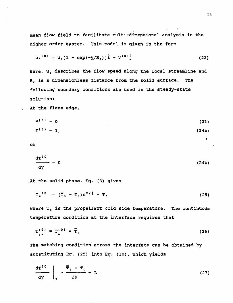
13

mean flow field to facilitate multi-dimensional analysis in the

higher order system. This model is given in the form

u, t 0 1 = ue[l - exp(-y/Re)ji + v(0)3 (22)

Here, uc describes the flow speed along the local streamline and

Rc is a dimensionless distance from the solid surface. The

following boundary conditions are used in the steady-state

solution:

At the flame edge,

Y(0> - 0 (23)

T(0) = 1. (24a)

or

dTio>0 (24b)

At the solid phase, Eg. (8) gives

Ts(0) = (Ts - TJeY/* + Tc (25)

where Tc is the propellant cold side temperature. The continuous

temperature condition at the interface requires that

T(0) „ T(0> 0

The matching condition across the interface can be obtained by

substituting Eq. (25) into Eq. (10), which yields

dT(o, m _ m1 3 •"• C

+ L (27)n

14

In solving Eg. (16) , note that a correct rate constant B in Eq.

(21) has to be determined such that the system satisfies the

boundary conditions at the flame edge as well as at the

interface.

Higher Order Governing Equations

The higher order governing equations can be expressed in a

single form because only the source terms are different from each

other. Presenting the source terms on the right-hand side of the

equations in terms of G8, the governing equations are represented

as follows:

Continuit

-i. / , V I I 4.+ (/» Ui + p

Momentum

(0) A(I) ( 0 > < 0 > A ( I ) « 0 ) A l I ) (0) A ( I ) ( 0 > (0)i lup Uj + [p u i y j U j + p u i , j U j + p u i , j u j

1 A ( I )

+ P i( I ) -1- A < I )

.. . - G2i (29)

Energy

iIup(0>T(I) +

*Y • 1A | v % A I i J ^ / T %

- ilw - P(I) - T/u - w(I)h = G3 (30)

Species

iIWp(0>Y(I>

15

A ( I )

- Y/n (31)

State

_ ( 0 ) m ( I ) _ A ( I ) ™ ( 0 ) _ r-p I -p T - G «

and the reaction rate is given by

(32)

w( 0 )2 A E

A ( I ) , £( I

( 0) ^ ' T( 0) 2

2

y( 0 >(33)

Here, G8 is given as follows: for the first order system (1= 1),

G = 0; for the second order system (I = 2),

2 i

G3 = -

p ( 1 J U ( i }

A • . • A

, , , . A ( 1 >

> U i , j U j

, i

( 0 ) A ( 1 )

( 0 )

A , , , ( 0 ) A ( j( 1 >i

A , , . A ( 0 )

rg = p( 1 ) m ( 1 )

W( 0)

( 0 )

( 1 > \ 2

( 0)

- 1

2E ( 1 > ( 1 >( 0 > T ( 0) 2 ^

ip( 1 )

rp( 0 )

2

4" ™ •y( 0 >T< 0) 2

< 0 ) v < 0)p *

y t 1 > £ ( 1 )

« 0 )

(34)

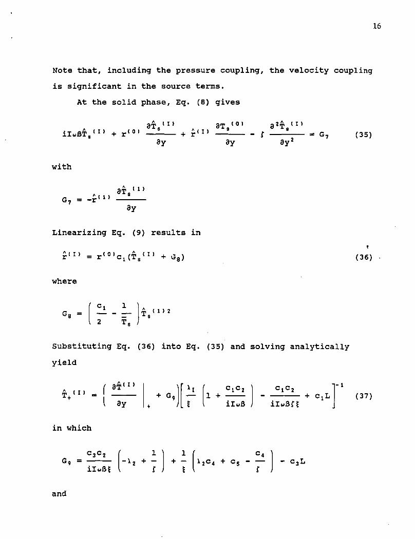
16

Note that, including the pressure coupling, the velocity coupling

is significant in the source terms.

At the solid phase, Eq. (8) gives

iIuBT8(J> + r( o ) a*,< i > ( 0 )

with

3T,_ r«i) 111

3y!(35)

Linearizing Eq. (9) results in

r « i > = r(0 i >

where

(1)2

2 T

t

(36)

Substituting Eq. (36) into Eq. (35) and solving analytically

yield

A r T iT ( I)

in which

3Tf _I ay

( I >

+ G« — 1 +ClC2

iluB

-l

(37)

cc3 2

il«flj- c,L

and

17

\l =

i - E8 /T82

1 _C, - - (T. - Tc)

c, = c, 1•3 ~ *-l

C4 .- -

1 A ( 1 ) 2

2

ip

c5- i2wfi

Equation (37) gives a boundary condition at the surface; other

conditions are as follows:

At the flame edge,

Y < x' = 0 (38)

Assumption of an isentropic flow near the flame edge gives the

temperature conditions. These conditions are equivalent to Eq.

(3) after deleting the thermal diffusion and reaction terms.

Noting that the steady-state temperature gradient at the flame

edge is almost zero, this condition can be expressed in the form

ir - 1.u

•y

with

18

'10

Since the flux of each reactant species is always a fixed

fraction of the total flux, the fuel mass flux fraction mf can be

derived from Eq. (4) as

- Y/M (40)

For a one-dimensional expression/ mf is given as

1 dYmf = Y

m dy

where m is the mass flux equal to pv, and assumption of the

constant burning rate at an instant has been used. At the

surface,

(41)

m, (i > 1 dY( I )

m < 0 > dy m (0)2m (i >

dY ( 0 )+ G

dy11 (42)

in which

m

1

( 0 )

m dY o >

m (o> dy dy

m1

m

) \ 2 n

o >

Using the relationship m 1 l' = p srl l ) yields

dY( dY ( 0 )- c,

dy dy

f\

(T8( I )

Gia) (43)

with

19

'12 - — T(1)2

The normal velocity component is derived from the mass

balance condition at the interface such that

(i >Eg

—T0- TSP

(I)13 (44)

where

m ac - V2T8

pi l> __ T—I T

Moreover, the parallel velocity component may be obtained using *

the Taylor series expansion about the surface where the no-slip

condition must be valid. Thus,

u. (i > 1 8u(0>

ilwfl

with

8y

i >

'13 (45)

2 ( 0 )9U

2 2 2

I > 2

2I*u*B< 3y'

Note that G7 - G14 are valid only for 1 = 2 . For higher order

systems, Egs. (37)-(39) and Egs. (43)-(45) are used as boundary

conditions to solve Egs. (28)-(32). It is necessary to have more

conditions for the density at both sides for better solutions,

and the pressure fluctuation has to be forced at the flame edge.

In the case of the second order time-independent system, care

must be taken to use boundary eguations (35) and (39).

20

3. NUMERICAL METHOD

Each set of governing equations, subject to appropriate

boundary conditions, is solved using the Galerkin finite element

method. The boundary equations are imbedded in the total matrix

equations by means of Lagrange multiplier XY, such that the

overall global matrix has the form

Xfl Ga(46)

in which Xfl represents the solution vector, Xfl *» [pfi, ufll, Tfi,

Yfl, Pfl], and Ga denotes the inhomogeneous source terms valid for

the second order. The second row, q-/flXfl = b-y represents the

boundary equations, where 7 - l,2,...,m, m being the number of

equations. The solution of Eq. (46) at a given frequency is

obtained by imposing the Dirichlet condition of the pressure at

the flame edge. Note that the first row of Eq. (46) gives the

eigenvalue problem when Ga = 0 and from which the natural

frequency of the system is obtained. The finite element

formulation contains two different kinds of test function used to

represent the volume and surface integrals in the domain. The

total number of field variables would be reduced by one if the

density or pressure were eliminated using the perfect gas law.

However, the stability of the matrix is doubtful. Before

calculations, the following is expected: since the Mach number

is generally very small, the coefficient of the pressure term in

Eq. (2) dominates the system unless the frequency considered is

large enough such that other coefficients containing the

21

frequency factor become comparable in magnitude. Therefore, in

lower frequencies the pressure gradient has to be negligible,

thus resulting in constant pressure. On the contrary, the

gradient will become significant in higher frequencies; this

results in pressure variance. In the latter case, severe

pressure changes will occur if unbounded at the solid surface.

Note that care must be exercised in expanding Eq. (9) due to the

appearance of the exponential growth effect. For the steady-

state case, as mentioned earlier, we calculate the eigenvalue B

in which necessary initial conditions are satisfied. However, as

will be discussed later, the eigenvalue is referred from the

result of reference [21] for this study.

4. DISCUSSION

All the perturbed governing equations in the higher order

systems having variable coefficients basically depend on the

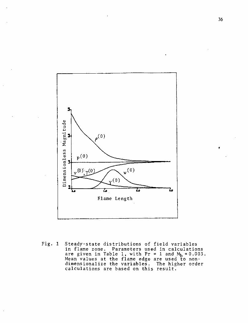
steady-state temperature distribution in the domain, as shown in

Eqs. (15)-(18). Figure 1 shows a typical steady-state

distribution of the field variables, including the reaction rate

for an adiabatic flame with a second order chemical reaction

mentioned in T'ien [21]. For verification, the following

parameters are utilized: z = 1, 8 = 0, Tc = 0.15, T8 = 0.35, f =

5 = 1 , E - 10, Eg = 4, L = 0.15, and fi = 1000. The other

parameters are taken from Flandro [23] and are as follows: "i =

1.2, Mb = 0.003, uc = 1.0, Rc = 5.0, Pr = 1.0, and h = 1.3.

Representative dimensional parameters corresponding to the

dimensionless values are given in Table 1.

Table 1 Typical value and range of parameters

22

TypicalParameter Value

Pa 1000

»g 1

Tc 0.15

T8 0.35

Tf 1.0

E 10

T3* ^

CP

m0 1

PO 1

^ 2

Yf 0.5

u "

1 1.4

AH 0.15

PhysicalRange Variable

250-1000 -g/cm3

g/cm3

°K

°K

°K

4-15 cal/gmole

2-10 cal/gmole

cal/g°k

cal/g°k

cal/cm°ksec

cal/cm°ksec

g/cm2 sec

atm

0.5-2

0.4-0.85

10"3-102 H2

0.05-0.3 cal/gmole

TypicalValue

1.5

1.5 x 10'3

300

700

2000

40 X 103 *

16 X 103

0.33

0.33

5 X 10~4

5 X 10~4

0.4

9.5

2.8 X 103

23

As mentioned earlier, the natual frequency of the given

system is obtained from the homogeneous solution of the total

matrix equation (46) without the boundary conditions. As

previously suggested [28], the result shows that the active

energy transfer between the acoustic wave and the combustion

process occurs mostly in a lower frequency range which leads to

acoustic instability. In this study, most of the frequencies are

clustered in w < 20; hence, the frequency range of interest is

chosen between u = 10"3 and w = 102 and it extends up to « » 500.

The thickness of the burning zone is assumed to be

negligibly small compared with the wavelength of the acoustic

oscillation; thus, the pressure is approximately uniform«

throughout the domain of study and varies only with time. From

this point of view, one of the most significant aspects of the

present study is the fact that the oscillating pressure is no

longer taken to be uniform at any instant, but is regarded as a

spatially nonhomogeneous time-dependent source term.

Consequently, it allows us to investigate the response of a

specific propellant at significantly high frequencies and to find

the response in the long flame of a double-base propellant. The

frequency limit has usually been determined by the reciprocal of

the characteristic time in Eq. (16). However, is is inversely

proportional to the square of the burning rate; therefore, the

limit cannot be constant, but varies with the pressure

fluctuations. This argument is verified in the present study

using two different cases: (l) increasing the order of

perturbation decreases the upper limit of the frequency and (2)

24

increasing the flame thickness also decreases the upper limit.

Flandro [23] defines the non-uniform pressure coefficient

explicitly in terms of the position and incident angle outside

the combustion region; however, further discussion concerning

this subject is not available.

First, we attempt to verify the results of the new model in

the one-dimensional problem. The calculation is actually

conducted in multiple dimensions, but the boundary conditions are

chosen approximately as if the gas flow seems to act one-

dimensionally. Data at the center nodes of the domain are used

to evaluate the results. Figure 2 demonstrates distributions of

component fluctuations in the first order at w = 1. The results

are comparable to those of T'ien [21]. In Fig. 2, it is also

shown that the highest temperature fluctuations arise at the

point where the maximum reaction occurs. Other field variables

have their maximum/minimum values at the point where the gradient

of the reaction is maximized. The temperature amplification at

the surface changes the burning rate in Eg. (36), while the

velocity at the flame edge represents the acoustic admittance,

whose magnitude and sign indicate the instability of the system.

Note that the pressure remains constant, implying that the

acoustic wavelength is larger than the flame thickness in this

case; consequently, the imaginary part of the velocity approaches

a constant slope at the edge.

Distributions of the field variables against frequency for

the first order are calculated and shown in Figs. 3-7. The

amplitude of the pressure disturbance playing the role of the

25

forcing function is set to unity at the- flame edge. The results

show that, at certain lower frequencies (« < 10), the pressure is

constant but varies in the higher region (« > 10). Thus, the

limit of the constant pressure assumption is clearly recovered.

General trends show that the distribution profiles are divided

roughly into two groups at about « = 1; one is for u < 1 and the

other for « > 1. In the lower frequencies (quasi-steady region),

the variables, keeping similar distribution profiles, change

their magnitude negligibly along the frequency. This trend is

also true for the higher frequencies up to w » 100. The only

exception is at w = 1, and it gives very different distribution

profiles among others. The figures also reveal that the results

are closely related to the chemical reaction distribution.

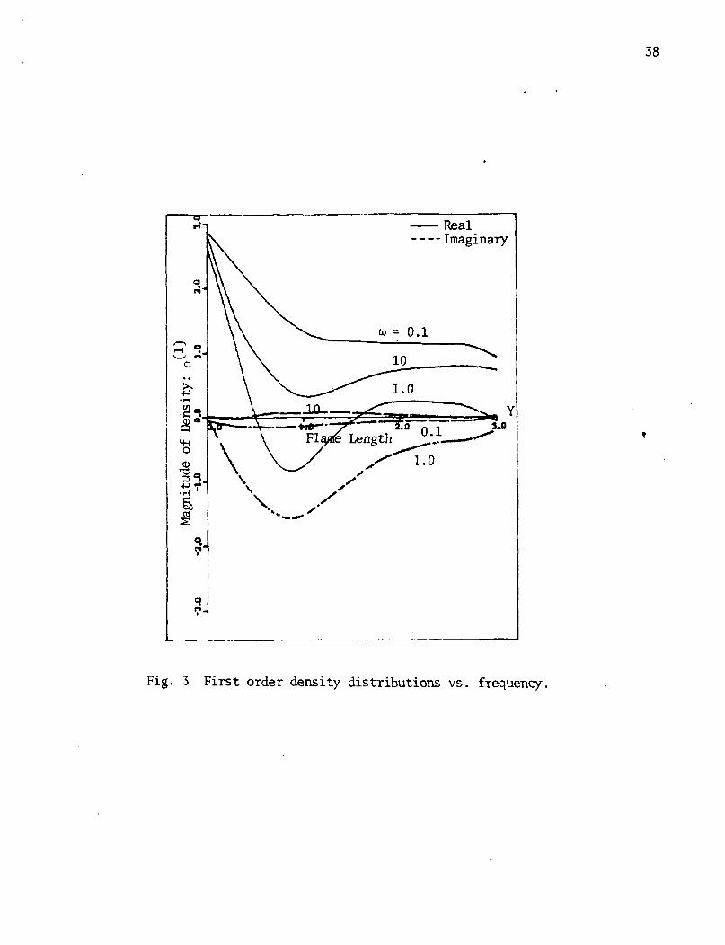
The overall density distributions based on a second order

chemical reaction are depicted in Fig. 3. The changes in

magnitude along the flame are more significant in higher

frequencies than in lower frequencies. These changes seem to be

directly related to the fuel species (Fig. 7) and implicitly

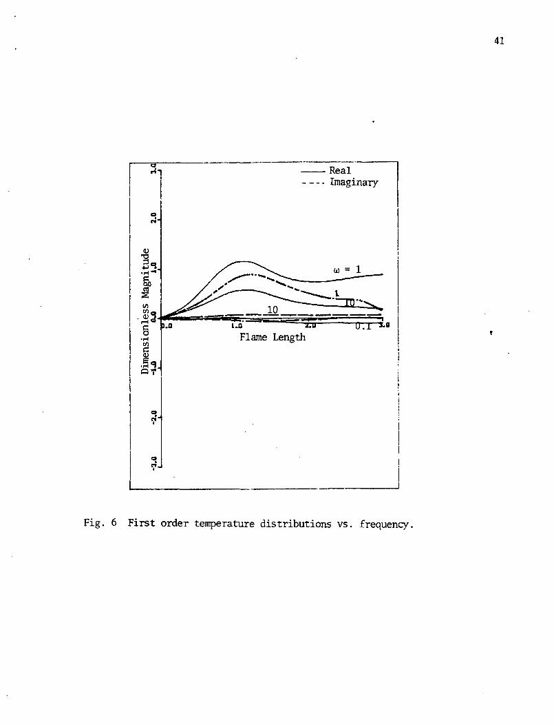
related to the temperature (Fig. 6). The imaginary parts of the

density represent the phase shift from the incident wave, and

these are almost zero except for u = 1.

At the surface, positive magnitude implies a stagnant

phenomena caused by decreasing the velocity, although the mass

flux increases at a higher pressure level. Special attention is

invited to the profile at w = 1, where the profile is entirely

different from others and some portions of the flame have

negative amplitudes. The mass balance predicts a faster velocity

26

at the negative portion, as shown in Fig. 4. It can be said that

the combustion system is most sensitive to the pressure

fluctuation at « = 1 in the frequency region considered. If the

upper limit of the frequency is extended, the profile is

reversed, but with a similar trend of periodicity. A simple

chemical reaction model restricts a realistic discussion in

detail since, for most propellants, it is more complex than it

implies.

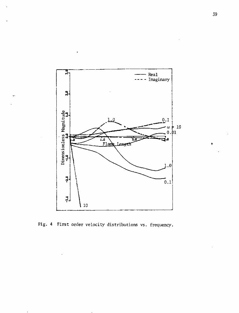
The normal velocity distributions are shown in Fig. 4. Two

kinds of profile are obvious: one with positive slope and one

with negative slope. The latter contains most of the

distributions in the lower frequency region, with some

exceptions. Note that a different profile appears at w = 1.

Rearranging the real part of the velocity at the flame edge gives

the distribution of the acoustic admittance, whose magnitude and

sign indicate the amplifications or damping ability of the flame

subject to the acoustic disturbance (Fig. 5). Figure 5 reveals a

resonance in the condensed phase near u = 0.01, indicating that

the system is unstable. This verifies the early result of

Denison and Baum [4]. Some negative peaks exist at the other

frequencies, indicating that the resonance in the gas phase tends

to damp the oscillatory motion. Figure 5 also shows the system

to be unstable at most higher frequency regions. The real part

of the burning rate in Eq. (36) gives a similar trend to the

acoustic admittance at the quasi-steady region, although the

magnitude is significantly different. But these trends differ

from each other at the higher region, as indicated in [21],

27

Thus, the burning rate is not representative as a stability

measure for a higher oscillatory case. Over w = 100, the profile

tends to have a second mode oscillation as the pressure varies in

the flame zone.

Figures 6 and 7 illustrate the temperature and fuel species.

At the lower frequency region, changes of magnitude are

insignificant while at the higher region, such changes become

significant. Because the temperature increases with fuel

consumption, the distribution curves are in opposing directions.

It is also seen that linearly diminishing the fuel affects the

temperature changes slowly. Note that the difference in the fuel

amount at the surface implies the change in the burning rate

affected by the disturbances. Significant changes of variables

are also given at w = 1.

In the first order system, the constant pressure field is

valid until w = 10; above that frequency the pressure varies.

This result gives the limit of the uniform pressure assumption.

Furthermore, it shows that up to w = 100, the magnitude grows

linearly starting from the flame edge where the Dirichlet

condition is imposed, and then begins to oscillate.

As previously indicated, each variable of the second order

response to acoustic disturbance has two components: one time-

dependent component that oscillates at twice the fundamental

frequency and one that is time-independent. The latter

represents a shift in the mean value, thus causing a shift of the

mean burning rate. The right-hand side of the second order total

matrix equation consists of corresponding nonlinearities in terms

28

of the product of two first order variables. These

nonlinearities function as source terms. The computations are

performed for the time-independent component using the Dirichlet

condition of the pressure to be unity at the flame edge.

Distributions of the field variables as well as the shift of the

burning rate are investigated. Figure 8 shows typical

distribution profiles in the second order at w = 1; at this

frequency, the constant pressure is retained.

The variables follow trends similar to those of the first

order, although the amplifications affected by the existence of

nonlinearities in the higher order are different. The trends

still show a small discrepancy at the flame edge as in the first

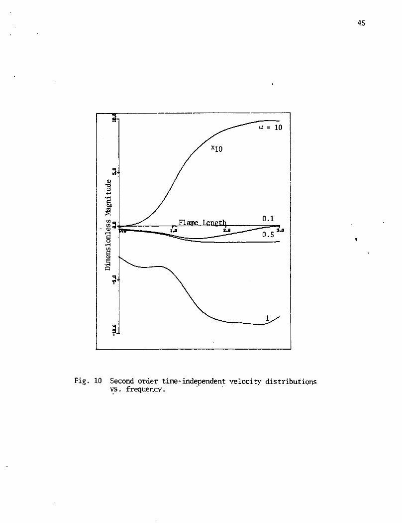
order. Figures 9-12 illustrate the behavior of each variable

against the frequency. The general tendency of the second order

is to affect the flame toward stability in the lower frequency

region. Note that the upper limit of the frequency for constant

pressure assumption has to be reduced by one half. The

computational results show that the pressure changes from u = 5,

which is half of the limit frequency in the first order. Thus,

the limit should be determined by considering the order of

perturbation involved in the calculations.

At w < 100, the variables have the same order of magnitude

as that of the pressure imposed. However, the velocity changes

significantly from w = 1 due to the pressure change from that

frequency. Thus, a higher order effect may not be negligible

unless the perturbation parameter e has an order of magnitude

less than the reciprocal of the highest order in the problem. At

29

lower frequencies, as shown in the first order, the distribution

profiles are very similar; at higher frequencies, they differ

from each other.

Finally, the burning rate offset is calculated and giv̂ .n in

Fig. 13. The offset is relatively small in the quasi-steady

region, but increases with oscillatory motion along the

frequencies. It has a negative sign in the entire frequency

range, indicating a decrease of the burning rate subject to the

acosutic pressure oscillations. This verifies the experimental

result of Price [39], and the averaged curve looks similar to the

analytical results of Friedly and Petersen [10].

Parameter studies are conducted for the first order and

summarized as follows. Decreasing the density ratio B affects

the variables shifted slightly to the negative direction, keeping

the distribution profiles constant. Changing the latent heat of

solid L exerts a negligible effect on the variables, but a very

small value of L shifts the system toward instability.

Increasing the surface activation energy E8 or the gas phase

activation energy E reduces the magnitude of the variables,

keeping the same profiles. Changes of the rate constant and

viscosity effect coefficient strongly affect the system, such

that every aspect discussed herein will change.

The present study could be extended to the multi-dimensional

case by introducing the appropriate axial mean flow field [46].

It is well recognized that fluctuation of the gas velocity

parallel to the propellant surface affects the burning rate in

terms of velocity coupling; therefore, this quantity must be

30

considered together with pressure coupling for a satisfactory

measure of stability. A simple calculation has been accomplished

using the artificial axial flow velocity in Eq. (22). However,

difficulties of the boundary conditions could not be eliminated.

A test run shows that the existence of a small amount of the

axial flow reduces the range of dispersion of the variable

distribution profile from each other in the frequency region that

leads the system toward stability.

5. CONCLUSION

A multi-dimensional numerical model for the premixed flame

acoustic instability is proposed and solved using the finite

element method. The governing equations are perturbed to the

second order and formulated with Galerkin finite elements. The

gaseous flame is assumed to be simple and homogeneous/ and the

Arrhcnius manner of decomposition is implemented with no

condensed phase reaction. The results have direct bearing on the

validity of published theories of solid propellant combustion

instability at the lower frequency region where the uniform

pressure is valid. Extended studies are made on the higher

frequency region and the results are discussed. Under the

restricted boundary conditions, the following conclusions, based

on numerical calculations, are reached:

(1) The pressure is assumed to vary in the domain of study, and

calculations based on nonuniform pressure indicate that for

w > 10, there is a significant deviation from the uniform

pressure assumption for the first order.

31

(2) For the second order system, such deviation occurs at a

lower frequency which is half of the first order frequency

limit.

(3) Investigation of the distribution of variables shows that

the acoustic instability is likely to be most critical at

u = 1, while the acoustic admittance at the flame edge

indicates a negative sign.

(4) The oscillatory amplification or damping ability of the

flame is recovered in the quasi-steady region and, at a

higher frequency, moderate amplification effects are

obtained.

(5) The burning rate is directly related to the acoustic

admittance only at the lower frequency region and its

negative offset phenomena have been valid in the second

order perturbation study.

(6) Second order effects may cause the instability to be more

critical in some cases and negligible in others.

(7) Multi-dimensional instability calculations can be achieved

using this model so far as a realistic mean flow field is

clarified with proper boundary conditions.

32

REFERENCES

1. Cheng, Sin-I, "High Frequency Combustion Instability inSolid Propellant Rockets", Jet Propulsion. 1954, Part I, pp.27-32, Part II, pp. 102-109.

2. Hart, R. W. and McClure, F. T., "Combustion Instability:Acoustic Interaction with a Burning Propellant Surface", J_._Chem. Phv.. Vol. 30, Sept. 1959, pp. 1501-1514.

3. McClure, F. T., Hart, R. W., and Bird, J. F., "AcousticResonance in Solid Propellant Rockets", J. APP!. Phvs.. Vol.31, Apr. 1960, pp. 884-896.

4. Denison, h. R. and Baum, E., "A Simplified Model of UnstableBurning in Solid Propellants", ARS J_._, Vol. 31, Aug. 1961,pp. 1112-1122.

5. Cheng, Sin-I, "Unstable Combustion in Solid PropellantRocket Motors", 8th Symposium (Int.) on Combustion, Williamsand Wilkins, 1962, pp. 81-96.

6. Williams, F. A., "Response of a Burning Solid to Small ?Amplitude Pressure Oscillations", J. Appl. Phys.. Vol. 33,NOV. 1962, pp. 3153-3166

7. Cantrell, R. H., Hart, R. W., and McClure, F. T., "LinearAcoustic Gains and Losses in Solid Propellant RocketMotors", AIAA J.., Vol. 2, No. 6, June 1964, pp. 1100-1105.

8. Hart, R. W. and McClure, F. T., "Theory of AcousticInstability in Solid Propellant Rocket Combustion", 10thSymposium (Int.) on Combustion, 1965.

9. Friedly, J. C. and Petersen, E. E., "Influence of CombustionParameters on Instability in Solid Propellant Motors, PartI: Development of Model and Linear Analysis", AIAA J.. Vol.4, No. 9, Sept. 1966, pp. 1605-1610.

10. Friedly, J. C. and Petersen, E. E., "Influence of CombustionParameters on Instability in Solid Propellant Motors, PartII: Nonlinear Analysis", AIAA J_.., Vol. 4, No. 11, Nov. 1966,pp. 1932-1937.

11. Culick, F. E. C., "Acoustic Oscillations in Solid PropellantRocket Chambers", Astronautica Acta, Vol. 12, Feb. 1966, pp.114-126.

12. Culick, F. E. C., "Calculations of the Admittance Functionfor a Burning Surface", Astronautica Acta. Vol. 13, No. 3,1967, pp. 221-237.

33

13. Culick, F. E. C., "A Review of Calculations for UnstableBurning of a Solid Propellant11, AIAA J.. Vol. 6, Dec. 1968,pp. 2241-2254.

14. Culick, F. E. C., "Nonlinear Behavior of Acoustic Waves inCombustion Chambers", CPIA Pub. 243, 10th JANNAF CombustionMeeting, Vol. 1, CPIA Pub. 243, 1973, pp. 417-436.

15. Ibiricu, M. M. and Krier, H., "Acoustic Amplification DuringSolid Propellant Combustion", Combustion and Flame. Vol. 19,1972, pp. 379-391.

16. Williams, F. A., "Quasi-Steady Gas-Phase Flame Theory inUnsteady Burning of a Homogeneous Solid Propellant", AIAA,£.., Vol. 11, 1973, pp. 1328-1330.

17. Levine, J. N. and Culick, F. E. C., "Nonlinear Analysis ofSolid Rocket Combustion Instability", AFRPL TR-74-45, Oct.1974.

18. Micci, M. M., Caveny, L. H., and Summerfield, M., "SolidPropellant Rocket Motor Response Evaluated by Means of ForceLongitudinal Waves", AIAA paper 77-974, July 1977.

19. King, M. K., "Modeling of Pressure-Coupled ResponseFunctions of Solid Propellants", 19th Symposium (Int.) onCombustion, The Combustion Institute, 1982, pp. 707-715.

20. Krier, H., T'ien, J. S., Sirignano, W. A., and Summerfield,M., "Nonsteady Burning Phenomena of Solid Propellant Theoryand Experiments", AIAA J_._, Vol. 6, No. 2, 1968, pp. 278-285.

21. T'ien, J. S., "Oscillatory Burning of Solid PropellantsIncluding Gas Phase Time Lag", Combustion Science andTechnology. Vol. 5, 1972, pp. 47-54.

22. Flandro, G. A., "Solid Propellant Acoustic AdmittanceCorrelations", Vibration and Sound. Vol. 36, 1974, pp. 297-312.

23. Flandro, G. A., "Nonlinear Time-Dependent Combustion of aSolid Rocket Propellant", 19th JANNAF Combustion Meeting,Oct. 1982.

24. Micheli, P. L. and Flandro, G. A., "Nonlinear Stability forTactical Motors Vol. Ill - Analysis of Nonlinear SolidPropellant Combustion Instability", AFRPL TR-85-017, Feb.1986.

25. Chung, T. J., Hackett, R. M., Kim, J. Y., and Radke, R., "ANew Approach to Combustion Instability Analysis for SolidPropellant Rocket Motors", 19th JANNAF Combustion Meeting,Oct. 1982.

34

26. Chung, T. J. and Kim, P. K., "A Finite Element Approach toResponse Function Calculations for Solid Propellant RocketMotors", AIAA paper 84-1433, June 1984.

27. Chung, T. J. and Kim, J. Y., "Two-Dimensional Combined ModelHeat Transfer by Conduction, Convection, and Radiation inEmitting, Absorbing, and Scattering Media - Solution byFinite Elements", J_.. Heat Transfer. Vol. 106, 1984, pp". 448-452.

28. Chung, T. J. and Kim, P. K., "Unsteady Response of BurningSurface in Solid Propellant Combustion", AIAA paper 85-0234,Jan. 1985.

29. Chung, T. J., Finite Elemenc Analysis in Fluid Dynamics.McGraw-Hill Book Co., 1978.

30. Williams, F. A. and Lengelle, G., "Simplified Model forEffect of Solid Heterogeneity on Oscillatory Combustion",Astronautica Acta, Vol. 14, Jan. 1968, pp. 97-118.

31. Condon, J. A., Osborn, J. R., and Click, R. L., "StatisticalAnalysis of Polydisperse, Heterogeneous PropellantCombustion: Nonsteady-State", 13th JANNAF Combustion 'Meeting, CPIA Pub. 281, Vol. 2, 1976, pp. 209-223.

32. Beckstead, M. W., "Combustion Calculations for CompositeSolid Propellants", 13th JANNAF Combustion Meeting, CPIAPub. 281, Vol. 2, 1976, pp. 299-312.

33. Cohen, N. S., "Response Function Theories that Account forSize Distribution Effects - A Review", AIAA J_._, Vol. ?.9, No.7, July 1981, pp. 907-912.

34. Culick, F. E. C., "Stability of Longitudinal Oscillationswith Pressure and Velocity Coupling in a Solid PropellantRocket", Combustion Science and Technology. Vol. 2, 1970,pp. 179-201.

35. Micheli, P. L., "Investigation of Velocity CoupledCombustion Instability", Aerojet Solid Propellant Co., AFRPLTR-76-100, Jan. 1977.

36. Condon, J. A., "A Model for the Velocity Coupling Responseof Composite Propellant", 16th JANNAF Combustion Meeting,CPIA Pub. 308, Dec. 1979.

37. Beckstead, M. W., "Report of the Workshop on VelocityCoupling", 17th JANNAF Combustion Meeting, CPIA pub. 324,NOV. 1980, pp. 195-210.

35

38. Brown, R. W., Waugh, R. C., Willoughby, P. G., and Dunlop,R., "Coupling between Velocity Oscillations and SolidPropellant Combustion", 19th JANNAF Combustion Meeting, CPIAPub. 366, Vol. 1, Oct. 1982, pp. 191-208.

39. Price, E. Q., Mathes, H. B., Crump, J. E., and McGie, M. R.,"Experimental Research in Combustion Instability of SolidPropellants", Combustion and Flame. Vol. 5, 1961, pp. 149-162.

40. Coates, R. L., Horton, M. D., and Ryan, N. W., "T-BurnerMethod of Determining the Acoustic Admittance of BurningPropellants", AIAA J.., Vol. 2, No. 6, June 1964, pp. 1119-1122.

41. Coates, R. L., Cohen, N. S., and Harvill, L. R., "AnInterpretation of L* Combustion Instability in Terms ofAcoustic Instability Theory", AIAA J., Vol. 5, No. 5, May1967, pp. 1097-1102.

42. Brown, R. S., Culick, F. E. C., and Zinn, B. T.,"Experimental Method for Combustion AdmittanceMeasurements", Experimental Diagnostics in Combustion of fSolids; AIAA Progress in Astronautics and Aeronautics. Vol.63, edited by T. L. Boggs and B. T. Zinn, AIAA, NY, 1979,pp. 191-220.

43. Baum, J. D., Levine, J. N., and Lovine, R. L., "Pulse-Triggered Instability in Solid Rocket Motors", AIAA J_.., Vol.22, No. 10, Oct. 1984, pp. 1413-1419.

44. Lovine, R. L., Baum, J. D., and Levine, J. N., "EjectaPulsing of Subscale Solid Propellant Rocket Motors", AIAAJ..., Vol. 23, No. 3, Mar. 1985, pp. 416-423.

45. Caveny, L. H., Collins, K. L., and Cheng, S. W., "DirectMeasurements of Acoustic Admittance Using Laser DopplerVelocimetry", AIAA JJL, Vol. 19, No. 7, July 1981, pp. 913-917.

46. Chung, T. J. and Sohn, J. L., "Interactions of CoupledAcoustic and Vortical Instability", AIAA J.., Vol. 24, No.10, Oct. 1986, pp. 1582-1596.

36

Flame Length

Fig. 1 Steady-state distributions of field variablesin flame zone. Parameters used in calculationsare given in Table 1, with Pr = 1 and Mb=0.003,Mean values at the flame edge are used to non-dimensionalize the variables. The higher ordercalculations are based on this result.

37

RealImaginary

Flame Length

Fig. 2 First order distributions of field variablesat co = 1.

38

RealImaginary

Fig. 3 First order density distributions vs. frequency.

39

RealImaginary

)1

0.1

10

10

Fig. 4 First order velocity distributions vs. frequency.

40

acoustic admittanceburning rate

Fig. 5 Acoustic admittance and burning rate vs. frequency.

41

RealImaginary

Fig. 6 First order temperature distributions vs. frequency.

42

Fig. 7 First order species ("fuel) distributions vs. frequency.

43

Fig. 8 Second order time-independent distributions of fieldvariables at u = 1.

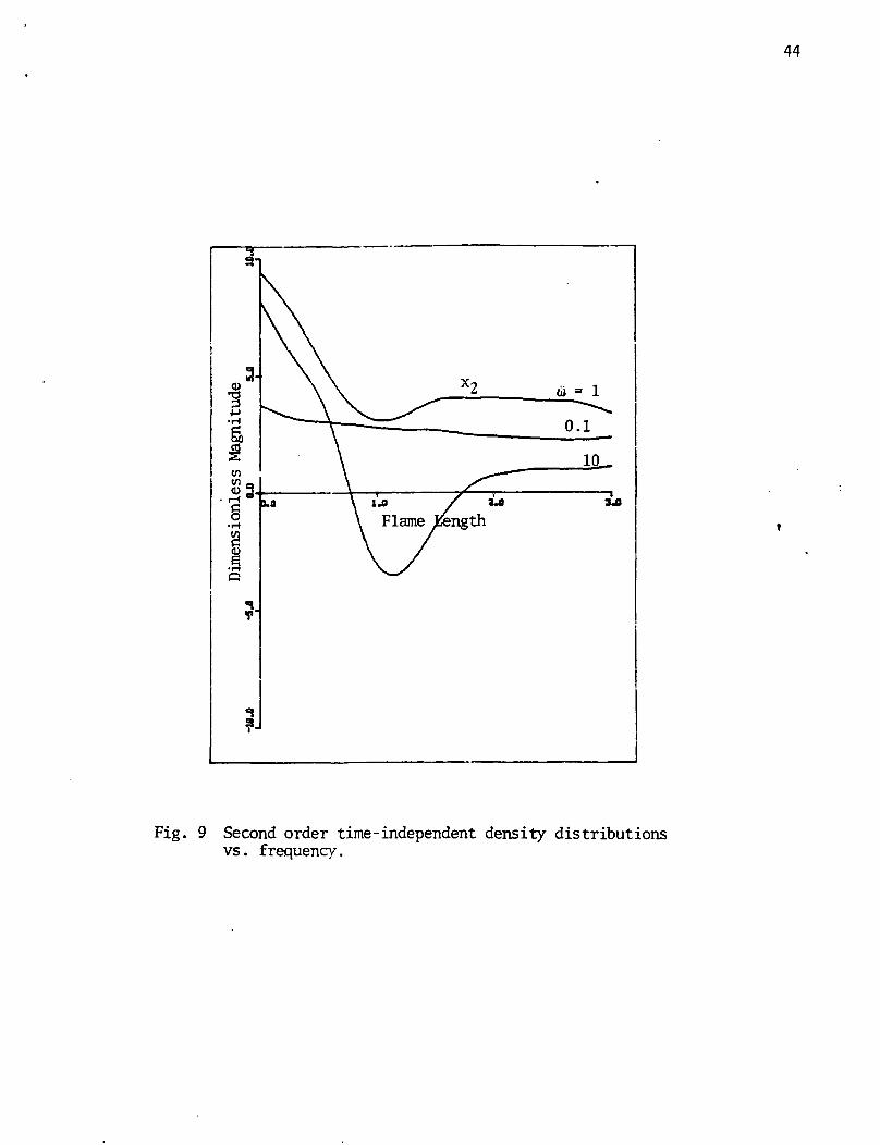
44

Fig. 9 Second order time-independent density distributionsvs. frequency.

45

3.0

Fig. 10 Second order time-independent velocity distributionsvs. frequency.

46

Fig. 11 Second order time-independent temperature distributionsvs. frequency.

47

§

0)

s

u = 0.13JJ

Fig. 12 Second order time-independent species (fuel) dis-tributions vs. frequency.

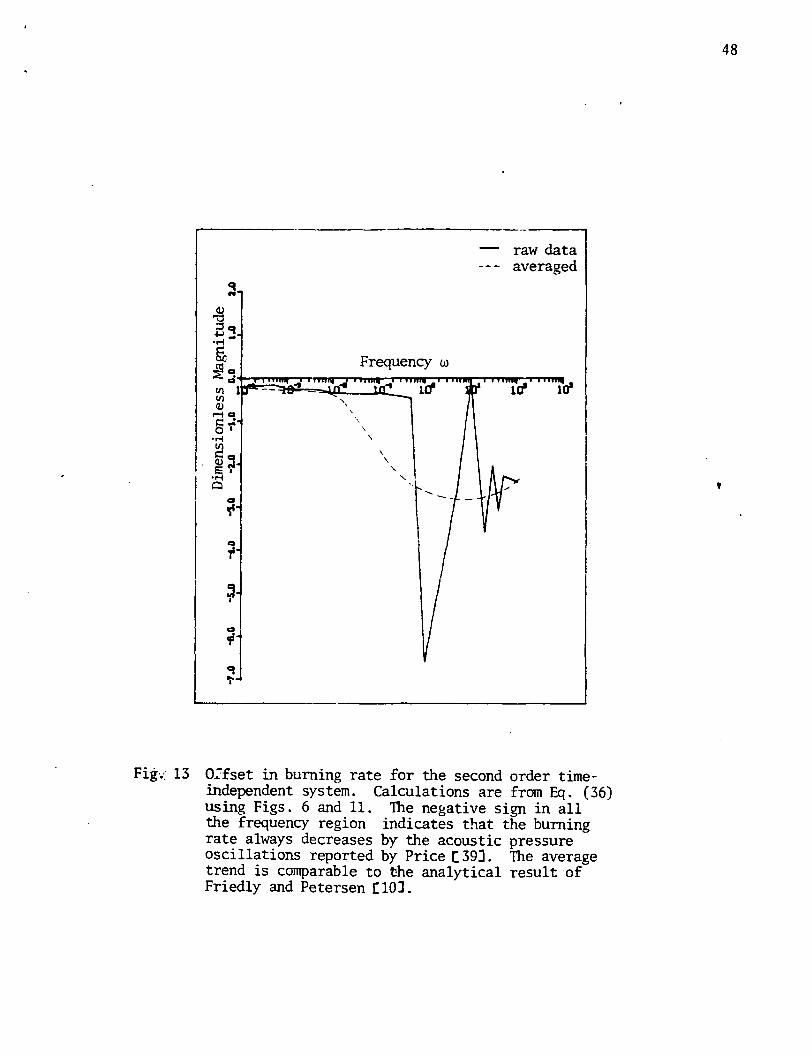
48

raw dataaveraged

I.•H "

&

C-O ••H

S3

Frequency to

Figv. 13 Orfset in burning rate for the second order time-independent system. Calculations are from Eq. (36)using Figs. 6 and 11. The negative sign in allthe frequency region indicates that the burningrate always decreases by the acoustic pressureoscillations reported by Price C393. The averagetrend is comparable to the analytical result ofFriedly and Petersen £103.