Learning from Manifold-Valued Data: An Application to

Seismic Signal Processing

by

Juan Ramirez Jr.

B.S.E., Electrical Engineering Purdue University Calumet, 2006

M.S., Mathematics Purdue University, 2008

A thesis submitted to the

Faculty of the Graduate School of the

University of Colorado in partial fulfillment

of the requirements for the degree of

Master of Science

Department of Electrical, Computer, and Energy Engineering

2012

This thesis entitled:Learning from Manifold-Valued Data: An Application to Seismic Signal Processing

written by Juan Ramirez Jr.has been approved for the Department of Electrical, Computer, and Energy Engineering

Francois G. Meyer

Shannon M. Hughes

Juan G. Restrepo

Date

The final copy of this thesis has been examined by the signatories, and we find that both thecontent and the form meet acceptable presentation standards of scholarly work in the above

mentioned discipline.

iii

Ramirez Jr., Juan (M.S., Electrical Engineering)

Learning from Manifold-Valued Data: An Application to Seismic Signal Processing

Thesis directed by Prof. Francois G. Meyer

Over the past several years, advances in sensor technology has lead to increases in the demand

for computerized methods for analyzing seismological signals. Central to the understanding of the

mechanisms generating seismic signals is the knowledge of the phases of seismic waves. Being able

to specify the type of wave leads to better performing seismic early warning systems and can also

aid in nuclear weapons testing ban treaty verification.

In this thesis, we propose a new method for the classification of seismic waves measured from

a three-channel seismograms. The seismograms are divided into overlapping time windows, where

each time-window is mapped to a set of multi-scale three-dimensional unitary vectors that describe

the orientation of the seismic wave present in the window at several physical scales. The problem of

classifying seismic waves becomes one of classifying points on several two-dimensional unit spheres.

We solve this problem by using kernel-based machine learning methods that are uniquely adapted

to the geometry of the sphere. The classification of the seismic wave relies on our ability to learn

the boundaries between sets of points on the spheres associated with the different types of seismic

waves. At each signal scale, we define a notion of uncertainty attached to the classification that

takes into account the geometry of the distribution of samples on the sphere. Finally, we combine

the classification results obtained at each scale into a unique label. We validate our approach using

a dataset of seismic events that occurred in Idaho, Montana, Wyoming, and Utah, between 2005

and 2006.

Dedication

To my wife.

v

Acknowledgements

I would like to express my gratitude to my research advisor, Professor Francois G. Meyer, for

his guidance, patience, and inspiration. Working with him has truly been a life changing experience.

I hope to one day follow in his footsteps and become a great teacher and mentor. I would also like

to thank Professor Shannon M. Hughes and Professor Juan G. Restrepo for being part of my thesis

committee. Finally, I would like to thank my family members and friends for their encouragement

and support.

vi

Contents

Chapter

1 Introduction 2

1.1 Seismological Signals . . . . . . . . . . . . . . . . . . . . . . . . . . . . . . . . . . . . 2

1.2 Seismic Sources . . . . . . . . . . . . . . . . . . . . . . . . . . . . . . . . . . . . . . . 4

1.2.1 Natural Seismic Sources . . . . . . . . . . . . . . . . . . . . . . . . . . . . . . 4

1.2.2 Artificial Seismic Sources . . . . . . . . . . . . . . . . . . . . . . . . . . . . . 9

1.3 Seismic Signal Parameters: Arrival Time & Phase . . . . . . . . . . . . . . . . . . . 9

1.3.1 Arrival Time . . . . . . . . . . . . . . . . . . . . . . . . . . . . . . . . . . . . 10

1.3.2 Seismic Phase . . . . . . . . . . . . . . . . . . . . . . . . . . . . . . . . . . . . 10

1.4 Our Contribution . . . . . . . . . . . . . . . . . . . . . . . . . . . . . . . . . . . . . . 11

1.4.1 Algorithm Overview . . . . . . . . . . . . . . . . . . . . . . . . . . . . . . . . 11

1.5 Scope and Overview . . . . . . . . . . . . . . . . . . . . . . . . . . . . . . . . . . . . 14

2 Feature Extraction 15

2.1 Phase Estimation Methods . . . . . . . . . . . . . . . . . . . . . . . . . . . . . . . . 15

2.1.1 Time Series Analysis . . . . . . . . . . . . . . . . . . . . . . . . . . . . . . . . 16

2.1.2 Spectral Methods . . . . . . . . . . . . . . . . . . . . . . . . . . . . . . . . . . 18

2.2 Geometric Polarization Analysis . . . . . . . . . . . . . . . . . . . . . . . . . . . . . 20

2.2.1 Physical Interpretation . . . . . . . . . . . . . . . . . . . . . . . . . . . . . . . 24

vii

3 Seismic Phase Learning 25

3.1 Supervised Learning . . . . . . . . . . . . . . . . . . . . . . . . . . . . . . . . . . . . 25

3.1.1 Supervised learning for Phase Classification . . . . . . . . . . . . . . . . . . . 25

3.2 Classifiers . . . . . . . . . . . . . . . . . . . . . . . . . . . . . . . . . . . . . . . . . . 26

3.2.1 Kernel Support Vector Machines . . . . . . . . . . . . . . . . . . . . . . . . . 27

3.2.2 Kernel Ridge Regression . . . . . . . . . . . . . . . . . . . . . . . . . . . . . . 28

3.2.3 k -Nearest Neighbors . . . . . . . . . . . . . . . . . . . . . . . . . . . . . . . . 29

3.3 Learning on the Sphere . . . . . . . . . . . . . . . . . . . . . . . . . . . . . . . . . . 30

3.3.1 Spherical Metric . . . . . . . . . . . . . . . . . . . . . . . . . . . . . . . . . . 31

3.4 Phase Classification on the Sphere . . . . . . . . . . . . . . . . . . . . . . . . . . . . 32

3.4.1 Mono-scale Classification . . . . . . . . . . . . . . . . . . . . . . . . . . . . . 32

3.4.2 Multi-Scale Classification . . . . . . . . . . . . . . . . . . . . . . . . . . . . . 35

4 Experimental Results 36

4.1 Data . . . . . . . . . . . . . . . . . . . . . . . . . . . . . . . . . . . . . . . . . . . . . 36

4.2 Preprocessing . . . . . . . . . . . . . . . . . . . . . . . . . . . . . . . . . . . . . . . . 38

4.3 Evaluation Strategy . . . . . . . . . . . . . . . . . . . . . . . . . . . . . . . . . . . . 38

4.4 Parameter Selection . . . . . . . . . . . . . . . . . . . . . . . . . . . . . . . . . . . . 40

4.5 Classification Results . . . . . . . . . . . . . . . . . . . . . . . . . . . . . . . . . . . . 42

4.6 Comparison of approaches . . . . . . . . . . . . . . . . . . . . . . . . . . . . . . . . . 44

5 Discussion and Conclusion 48

5.1 Discussion . . . . . . . . . . . . . . . . . . . . . . . . . . . . . . . . . . . . . . . . . . 48

5.2 Future Work . . . . . . . . . . . . . . . . . . . . . . . . . . . . . . . . . . . . . . . . 50

5.3 Conclusion . . . . . . . . . . . . . . . . . . . . . . . . . . . . . . . . . . . . . . . . . 51

Bibliography 52

viii

Tables

Table

1.1 Number of Earthquakes Worldwide from 2004 to 2011 . . . . . . . . . . . . . . . . . 5

1.2 Number of Earthquakes in the United States from 2004 to 2011 . . . . . . . . . . . . 7

4.1 Supervised Learning: Lg wave vs. Pn wave (% correct) adaptive σ method. . . . . 45

4.2 Supervised Learning: Lg wave vs. Pg wave (% correct) adaptive σ method. . . . . 45

4.3 Supervised Learning: Lg wave vs. Pn wave (% correct) constant σ method. . . . . 46

4.4 Supervised Learning: Lg wave vs. Pg wave (% correct) constant σ method. . . . . 46

4.5 Detection of the P and L waves using a hypothesis test. . . . . . . . . . . . . . . . . 47

ix

Figures

Figure

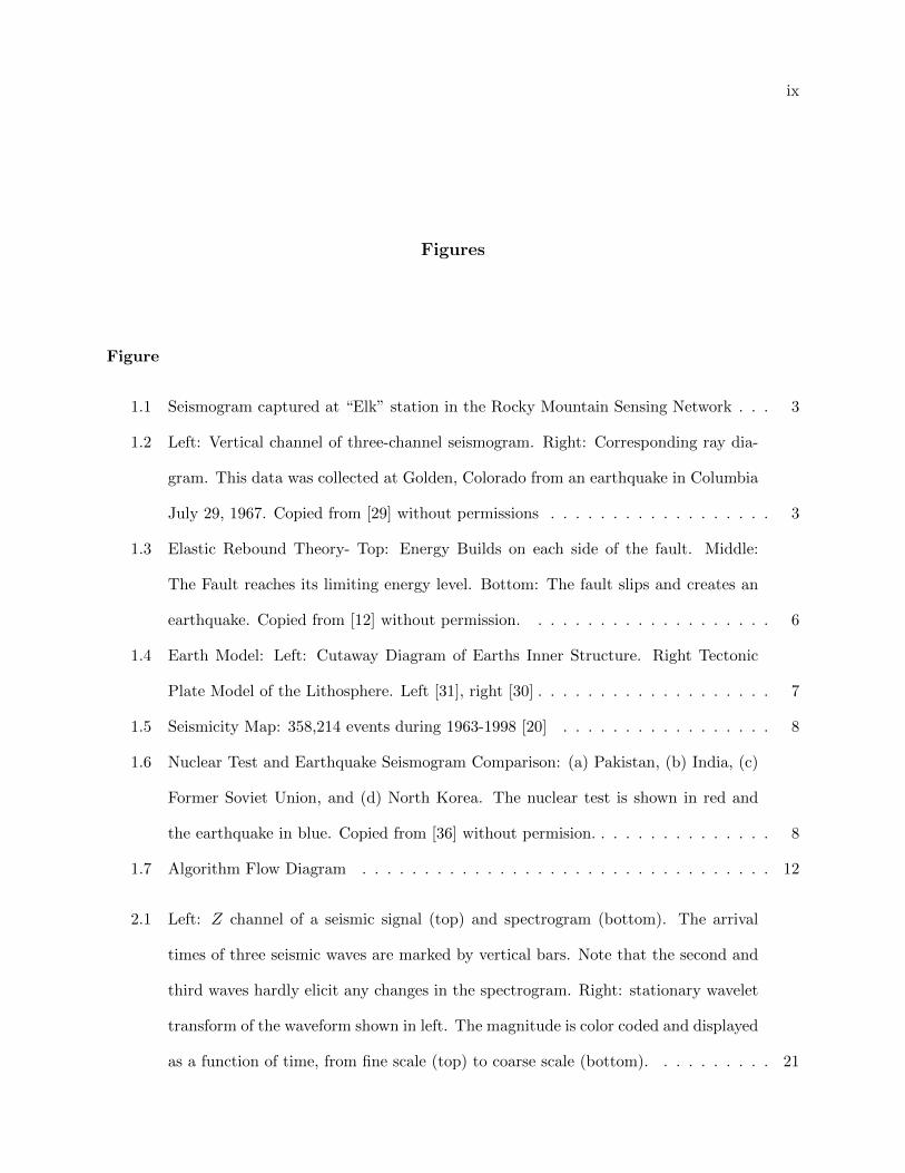
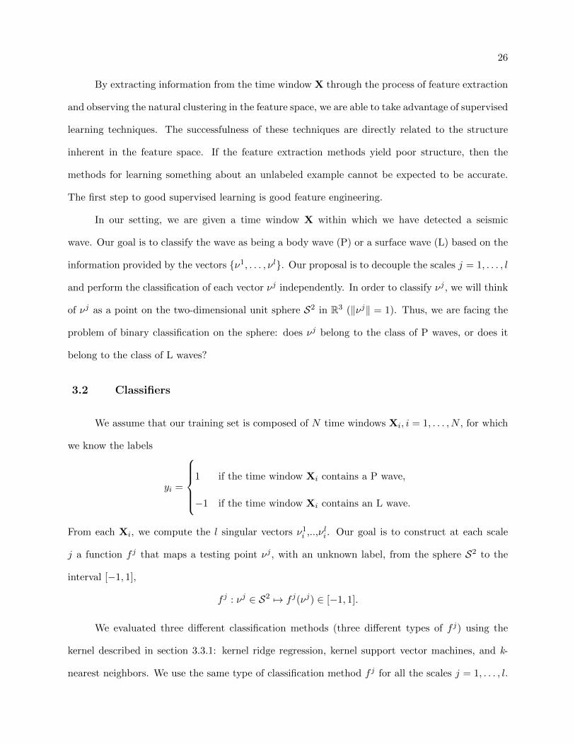
1.1 Seismogram captured at “Elk” station in the Rocky Mountain Sensing Network . . . 3

1.2 Left: Vertical channel of three-channel seismogram. Right: Corresponding ray dia-

gram. This data was collected at Golden, Colorado from an earthquake in Columbia

July 29, 1967. Copied from [29] without permissions . . . . . . . . . . . . . . . . . . 3

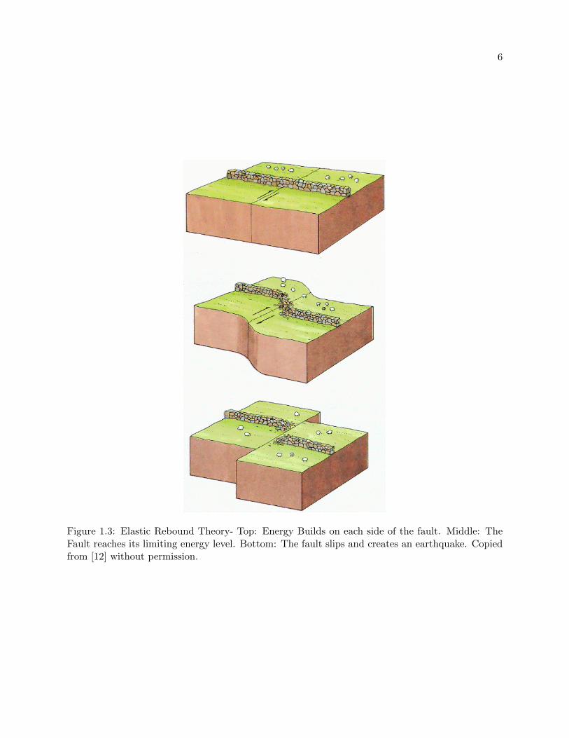
1.3 Elastic Rebound Theory- Top: Energy Builds on each side of the fault. Middle:

The Fault reaches its limiting energy level. Bottom: The fault slips and creates an

earthquake. Copied from [12] without permission. . . . . . . . . . . . . . . . . . . . 6

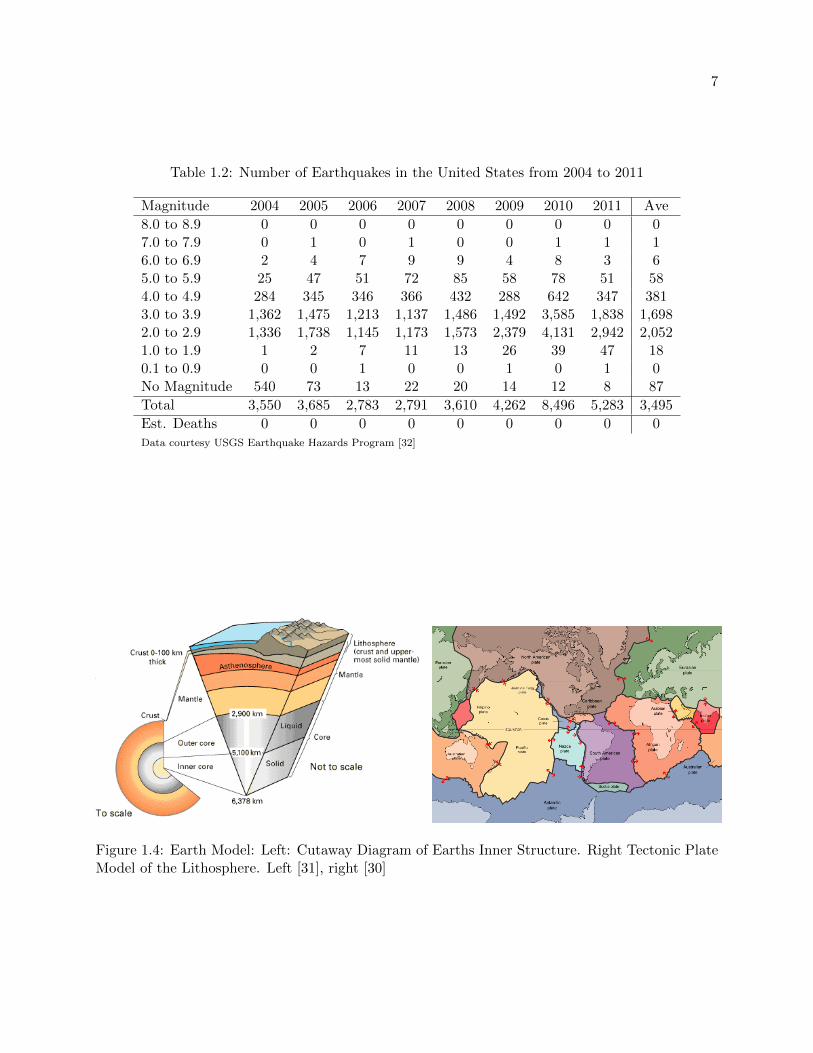
1.4 Earth Model: Left: Cutaway Diagram of Earths Inner Structure. Right Tectonic

Plate Model of the Lithosphere. Left [31], right [30] . . . . . . . . . . . . . . . . . . . 7

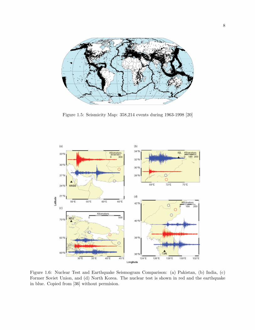
1.5 Seismicity Map: 358,214 events during 1963-1998 [20] . . . . . . . . . . . . . . . . . 8

1.6 Nuclear Test and Earthquake Seismogram Comparison: (a) Pakistan, (b) India, (c)

Former Soviet Union, and (d) North Korea. The nuclear test is shown in red and

the earthquake in blue. Copied from [36] without permision. . . . . . . . . . . . . . . 8

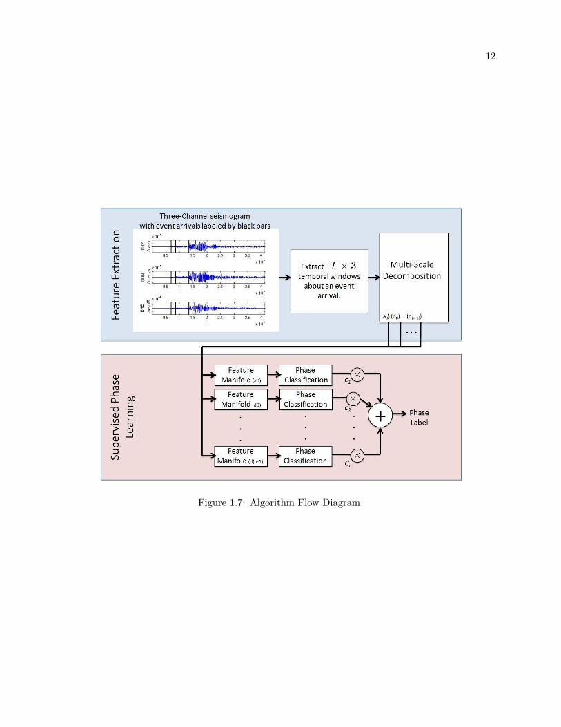
1.7 Algorithm Flow Diagram . . . . . . . . . . . . . . . . . . . . . . . . . . . . . . . . . 12

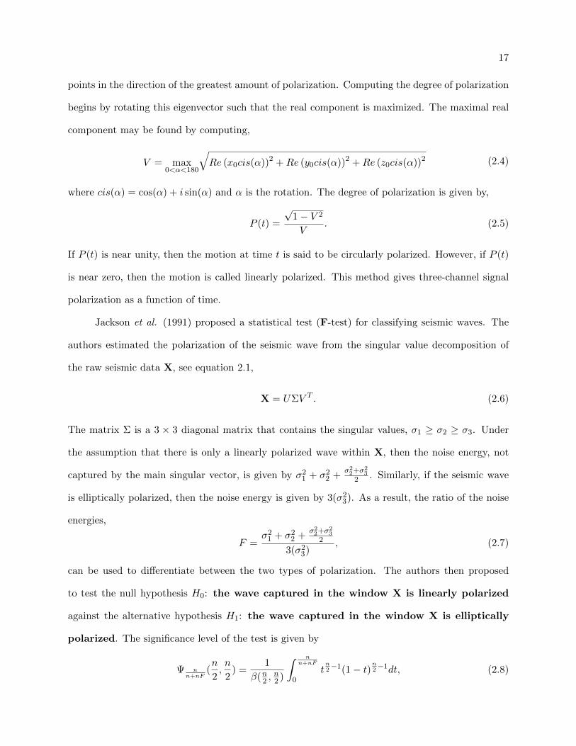
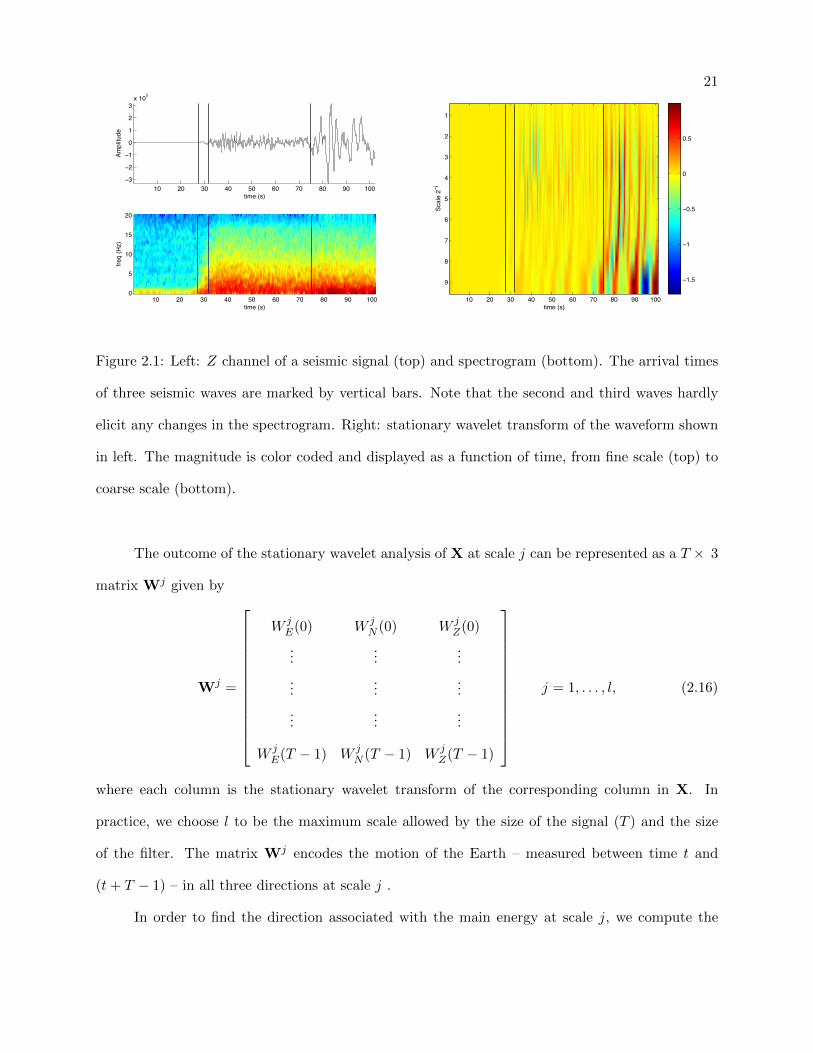
2.1 Left: Z channel of a seismic signal (top) and spectrogram (bottom). The arrival

times of three seismic waves are marked by vertical bars. Note that the second and

third waves hardly elicit any changes in the spectrogram. Right: stationary wavelet

transform of the waveform shown in left. The magnitude is color coded and displayed

as a function of time, from fine scale (top) to coarse scale (bottom). . . . . . . . . . 21

x

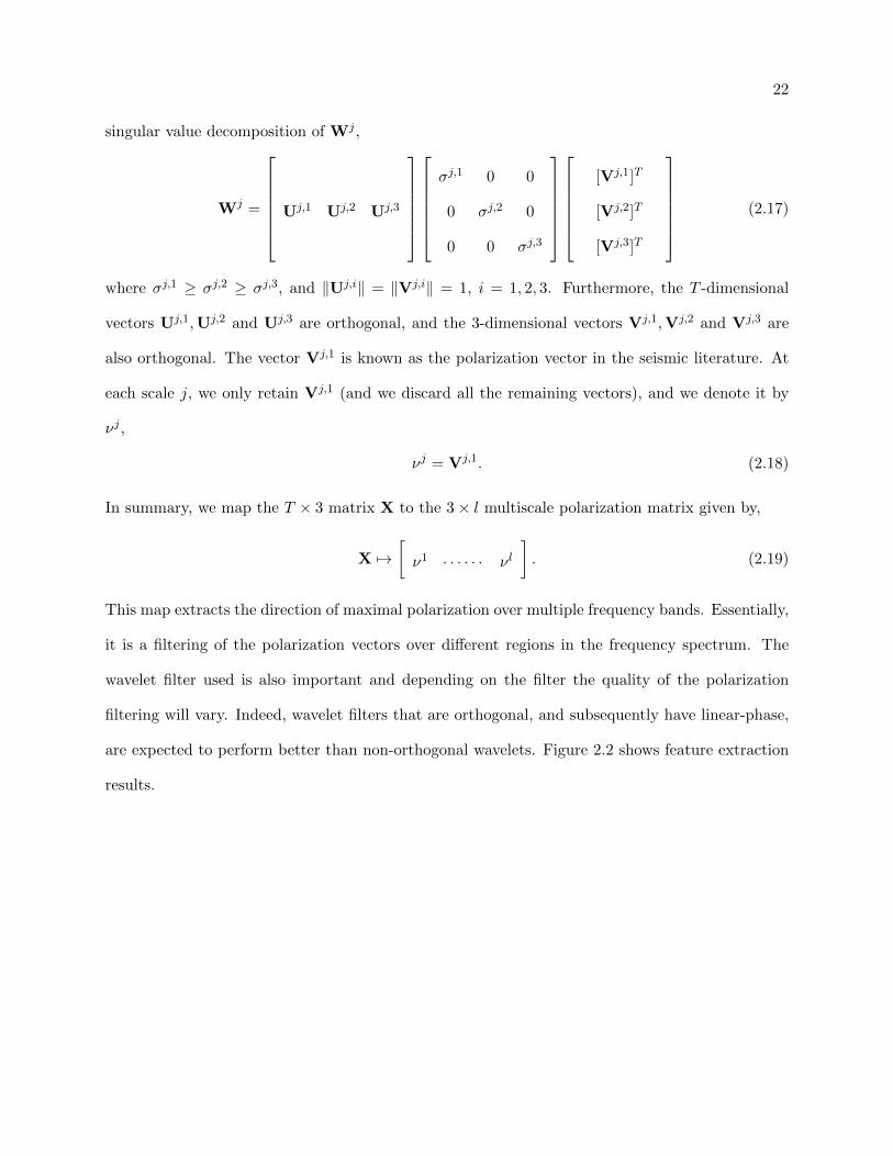
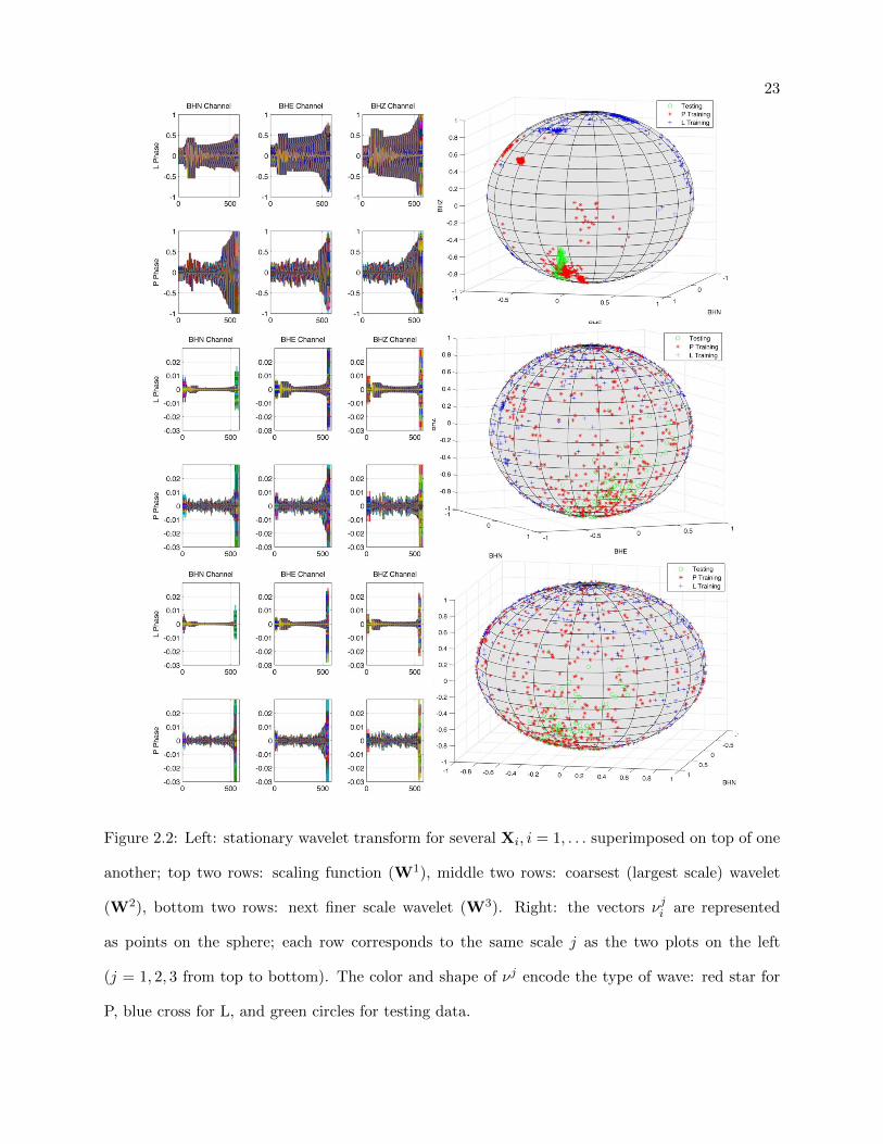
2.2 Left: stationary wavelet transform for several Xi, i = 1, . . . superimposed on top of

one another; top two rows: scaling function (W1), middle two rows: coarsest (largest

scale) wavelet (W2), bottom two rows: next finer scale wavelet (W3). Right: the

vectors νji are represented as points on the sphere; each row corresponds to the same

scale j as the two plots on the left (j = 1, 2, 3 from top to bottom). The color and

shape of νj encode the type of wave: red star for P, blue cross for L, and green circles

for testing data. . . . . . . . . . . . . . . . . . . . . . . . . . . . . . . . . . . . . . . 23

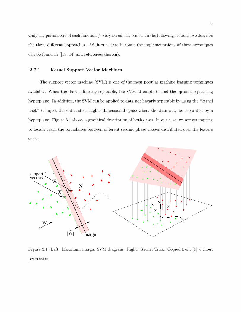
3.1 Left: Maximum margin SVM diagram. Right: Kernel Trick. Copied from [4] without

permission. . . . . . . . . . . . . . . . . . . . . . . . . . . . . . . . . . . . . . . . . . 27

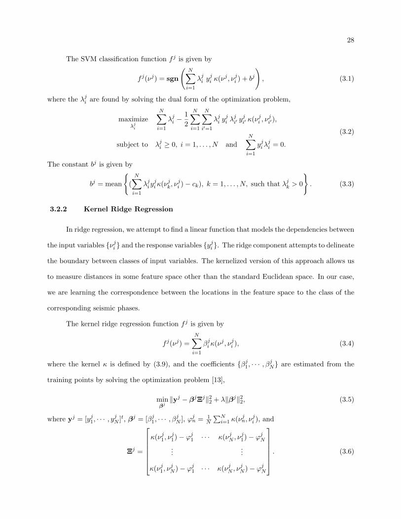
3.2 Illustration of the stiffness interpretation of the regularization parameter λ. Dashed

line represents a low stiffness value and the solid line represents a high stiffness line.

Copied form [4] without permission. . . . . . . . . . . . . . . . . . . . . . . . . . . . 29

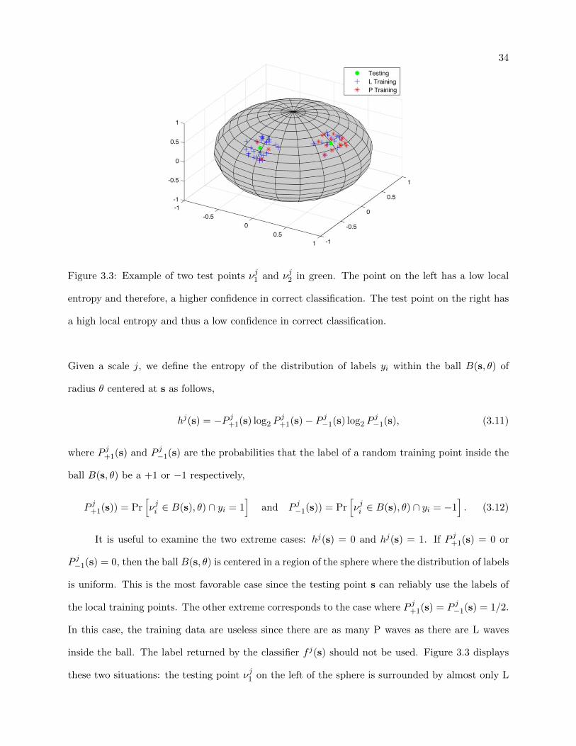
3.3 Example of two test points νj1 and νj2 in green. The point on the left has a low local

entropy and therefore, a higher confidence in correct classification. The test point on

the right has a high local entropy and thus a low confidence in correct classification. 34

4.1 Map of Rocky Mountain Seismic Sensing Network . . . . . . . . . . . . . . . . . . . 37

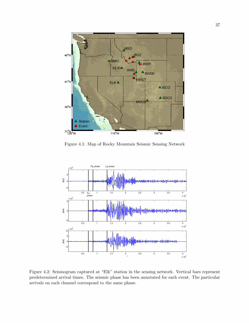
4.2 Seismogram captured at “Elk” station in the sensing network. Vertical bars represent

predetermined arrival times. The seismic phase has been annotated for each event.

The particular arrivals on each channel correspond to the same phase. . . . . . . . . 37

4.3 Plot of Kernel, see eqn. 3.9, leftmost curve corresponds to a σ = 0.04 and a radius

θνj = 12 while the rightmost curve corresponds to a σ = 0.59 and a radius θνj = 3π

4 . 41

1

Accomplishments

The work presented in this thesis has lead to the following presentations, publications, journal

submissions, and awards.

• J. Ramirez Jr. and F.G. Meyer. Machine Learning for Seismic Signal Processing: Phase

classification on a manifold. In Proceedings 2011 10th International Conference on Machine

Learning and Applications, pages 382-388. IEEE, 2011

• Pattern Recongnition Letters Elsevier, Spring 2012. submitted

• 2011 Society for the Advancement of Chicanos and Native Americans in Science Best

Applied Mathematics Graduate Student Presentation Award, presented at 2011 National

Conference, San Jose CA.

• Poster Presenter - 2011 Computational Optics Sensing and Imaging (COSI) Industrial

Board Meeting, Boulder CO.

• Poster Presenter- 2011 Purdue University Machine Learning Summer School, West Lafayette

IN.

Chapter 1

Introduction

1.1 Seismological Signals

Seismology is a field of study focused on developing an understanding of the Earth’s inner

structure through the analysis of Earth ground motion recordings, or seismograms. There is a

strong analogy between seismology and the study of sound waves. A seismic wave is generated at a

source, travels through a medium, and is collected by a recording device. Similarly, a sound wave

is generated by a source (e.g. a person or a tree falling in the forest), travels through the air, and

is received by the human ear. The study of such signals can provide information on the location of

the source and the medium through which the wave has traveled.

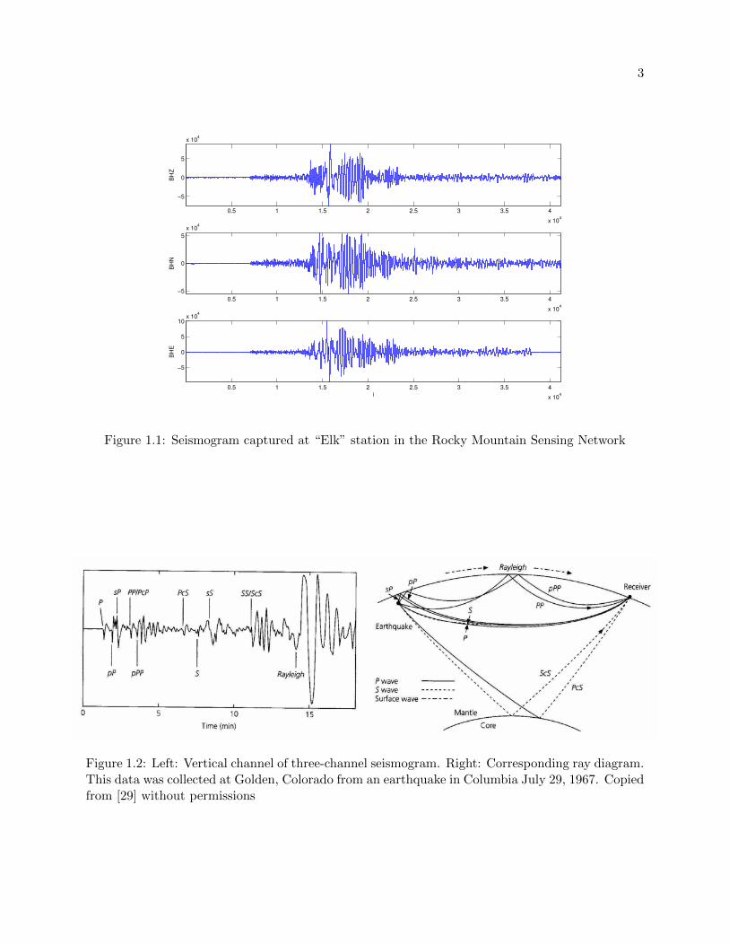
A typical seismogram is composed of three time series that measures the motion of the Earth

along two horizontal directions (E and N) parallel to the ground and a vertical direction (Z)

perpendicular to the ground. Figure 1.1 shows a sample three-channel seismogram. These seismic

waveforms are made up of several wave packets. Each wave packet (or phase, as noted in the

seismology literature) corresponds to a different type of motion with a different propagation path

through the Earth. Examples of such waves include body waves (e.g. P and S waves), which

travel through the Earth’s interior, and surface waves (e.g. L and R waves), which propagate

along the surface of the Earth. Figure 1.2 shows the vertical channel (Z) of a seismogram and its

corresponding ray path diagram. The ray path diagram plots the direction a seismic wave travels

through the Earth.

Over the past 60 years, the analysis of seismic signals has led to a deeper understanding of the

3

0.5 1 1.5 2 2.5 3 3.5 4

x 104

−5

0

5

x 104

BH

Z

0.5 1 1.5 2 2.5 3 3.5 4

x 104

−5

0

5

x 104

BH

N

0.5 1 1.5 2 2.5 3 3.5 4

x 104

−5

0

5

10x 10

4

i

BH

E

Figure 1.1: Seismogram captured at “Elk” station in the Rocky Mountain Sensing Network

Figure 1.2: Left: Vertical channel of three-channel seismogram. Right: Corresponding ray diagram.This data was collected at Golden, Colorado from an earthquake in Columbia July 29, 1967. Copiedfrom [29] without permissions

4

evolution of our planet, allowed nations to explore territories for underground natural resources, and

provided data useful for mitigating the effects of earthquakes on the human population. The focus

of this thesis is on methods for analyzing seismic signals for the purpose of extracting information

useful in mitigating the effects of earthquakes on society. These methods may lead to advances

in Early Seismic Warning Systems (ESWS) technology and provide a different perspective on the

analysis of seismic waves. In particular, we present an approach for the classification of seismic

phases using machine learning techniques.

In the remainder of this chapter, we describe seismic sources, discuss the fundamental pa-

rameters for source characterization and localization, and provide an overview of our approach to

seismic phase classification.

1.2 Seismic Sources

Seismic recording stations collect signals originating from two major classes of sources: nat-

ural and artificial. Natural sources refer to seismic waves originating from within the Earth, such

as earthquakes. These waves occur naturally as energy is released in the Earth’s lithosphere. On

the other hand, artificial sources refer to waves generated as a result of explosions. A primary

concern in the world community is the monitoring of nuclear weapons testing. In both cases, the

development of algorithms to rapidly characterize incoming seismic waves is a critical issue.

1.2.1 Natural Seismic Sources

Earthquakes are the result of energy release occurring in the Earth’s lithosphere. In particu-

lar, they occur primarily on fault lines, which are surfaces in the Earth where materials on one side

moves opposite to the other. A scientific notion called Elastic-Rebound-Theory has been widely

used to describe how earthquakes are generated. This theory was developed by Harry Fielding

Reid following the 7.8 magnitude San Francsico earthquake on the San Andreas fault in 1908. This

theory states that while materials on opposing sides of a fault move opposite to each other, the

friction on the fault locks the sides together preventing motion. Eventually, the forces built up

5

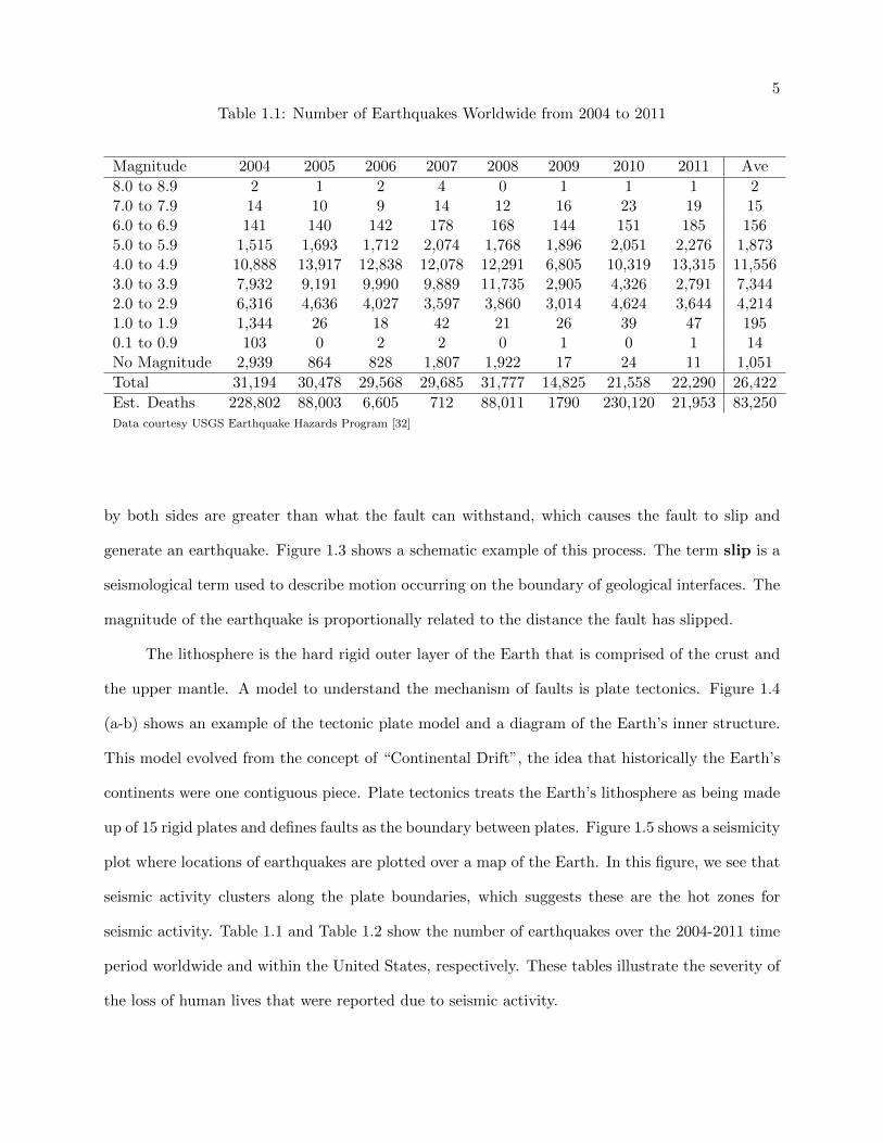
Table 1.1: Number of Earthquakes Worldwide from 2004 to 2011

Magnitude 2004 2005 2006 2007 2008 2009 2010 2011 Ave

8.0 to 8.9 2 1 2 4 0 1 1 1 27.0 to 7.9 14 10 9 14 12 16 23 19 156.0 to 6.9 141 140 142 178 168 144 151 185 1565.0 to 5.9 1,515 1,693 1,712 2,074 1,768 1,896 2,051 2,276 1,8734.0 to 4.9 10,888 13,917 12,838 12,078 12,291 6,805 10,319 13,315 11,5563.0 to 3.9 7,932 9,191 9,990 9,889 11,735 2,905 4,326 2,791 7,3442.0 to 2.9 6,316 4,636 4,027 3,597 3,860 3,014 4,624 3,644 4,2141.0 to 1.9 1,344 26 18 42 21 26 39 47 1950.1 to 0.9 103 0 2 2 0 1 0 1 14No Magnitude 2,939 864 828 1,807 1,922 17 24 11 1,051

Total 31,194 30,478 29,568 29,685 31,777 14,825 21,558 22,290 26,422

Est. Deaths 228,802 88,003 6,605 712 88,011 1790 230,120 21,953 83,250Data courtesy USGS Earthquake Hazards Program [32]

by both sides are greater than what the fault can withstand, which causes the fault to slip and

generate an earthquake. Figure 1.3 shows a schematic example of this process. The term slip is a

seismological term used to describe motion occurring on the boundary of geological interfaces. The

magnitude of the earthquake is proportionally related to the distance the fault has slipped.

The lithosphere is the hard rigid outer layer of the Earth that is comprised of the crust and

the upper mantle. A model to understand the mechanism of faults is plate tectonics. Figure 1.4

(a-b) shows an example of the tectonic plate model and a diagram of the Earth’s inner structure.

This model evolved from the concept of “Continental Drift”, the idea that historically the Earth’s

continents were one contiguous piece. Plate tectonics treats the Earth’s lithosphere as being made

up of 15 rigid plates and defines faults as the boundary between plates. Figure 1.5 shows a seismicity

plot where locations of earthquakes are plotted over a map of the Earth. In this figure, we see that

seismic activity clusters along the plate boundaries, which suggests these are the hot zones for

seismic activity. Table 1.1 and Table 1.2 show the number of earthquakes over the 2004-2011 time

period worldwide and within the United States, respectively. These tables illustrate the severity of

the loss of human lives that were reported due to seismic activity.

6

Figure 1.3: Elastic Rebound Theory- Top: Energy Builds on each side of the fault. Middle: TheFault reaches its limiting energy level. Bottom: The fault slips and creates an earthquake. Copiedfrom [12] without permission.

7

Table 1.2: Number of Earthquakes in the United States from 2004 to 2011

Magnitude 2004 2005 2006 2007 2008 2009 2010 2011 Ave

8.0 to 8.9 0 0 0 0 0 0 0 0 07.0 to 7.9 0 1 0 1 0 0 1 1 16.0 to 6.9 2 4 7 9 9 4 8 3 65.0 to 5.9 25 47 51 72 85 58 78 51 584.0 to 4.9 284 345 346 366 432 288 642 347 3813.0 to 3.9 1,362 1,475 1,213 1,137 1,486 1,492 3,585 1,838 1,6982.0 to 2.9 1,336 1,738 1,145 1,173 1,573 2,379 4,131 2,942 2,0521.0 to 1.9 1 2 7 11 13 26 39 47 180.1 to 0.9 0 0 1 0 0 1 0 1 0No Magnitude 540 73 13 22 20 14 12 8 87

Total 3,550 3,685 2,783 2,791 3,610 4,262 8,496 5,283 3,495

Est. Deaths 0 0 0 0 0 0 0 0 0Data courtesy USGS Earthquake Hazards Program [32]

Figure 1.4: Earth Model: Left: Cutaway Diagram of Earths Inner Structure. Right Tectonic PlateModel of the Lithosphere. Left [31], right [30]

8

Figure 1.5: Seismicity Map: 358,214 events during 1963-1998 [20]

Figure 1.6: Nuclear Test and Earthquake Seismogram Comparison: (a) Pakistan, (b) India, (c)Former Soviet Union, and (d) North Korea. The nuclear test is shown in red and the earthquakein blue. Copied from [36] without permision.

9

1.2.2 Artificial Seismic Sources

Artificial events occur from various sources, ranging from falling trees to nuclear weapons

testing. The case of primary concern is that of weapons testing. In 1963, 116 nations signed the

Limited Test Ban Treaty, which banned the detonation of nuclear weapons in the atmosphere,

ocean, and outer space. During this period in history, the World Wide Standardized Seismographic

Network (WWSSN) was deployed to primarily monitor nuclear testing. This system is credited with

being the driving force behind advances in seismic signal processing because it has provided valuable

data for research. In 1996, the United Nations General Assembly adopted a Comprehensive Nuclear

Test-Ban Treaty, which prohibits the detonation of any nuclear weapon of any load. However, this

treaty has not been successfully enacted since all 193 General Assembly member states have not

signed and ratified the treaty.

As a result, an active area of seismology research is that of identifying nuclear explosions.

This work has led to the identification of characterizing factors in the differences between nuclear

explosions and natural earthquakes. It is known that explosions induce motions that tend away from

the source, which subsequently produce much less shear wave energy. Since earthquakes originate

from slips on faults they produce large amounts of shear wave energy. This contrast forms the basis

for the methodology used to discriminate between natural and artificial seismic activity. Figure 1.6

shows an example of both natural and artificial seismic events.

1.3 Seismic Signal Parameters: Arrival Time & Phase

Techniques for the detection and identification of different types of waves are fundamental to

characterize the type (earthquake, explosion,...), location, and magnitude of a seismic event. In this

section, we will explore common techniques for detection of the arrival time and phase identification

of a seismic wave.

10

1.3.1 Arrival Time

The arrival time of a seismic wave refers to the the moment in the seismogram where the

signal energy crosses a user-determined threshold for detection. A classical method for arrival time

detection is called the current-value-to-predicted-value ratio method ([21], [1], [8], and references

therein). The current-value is determined by computing the short term average (STA) of incoming

seismic data while the predicted-value is the long term average (LTA). In essence, two real-time

data buffers are being populated with seismic data, with one of shorter length than the other.

If the STA/LTA ratio exceeds a specific threshold, an arrival is declared. This technique is the

gold-standard for seismic activity detection [33].

1.3.2 Seismic Phase

The phase of a seismic wave is a label given to each instance of seismic activity that char-

acterizes the wave as either (1) a compression wave (e.g. P-wave), shear wave (e.g. S-wave), or

surface wave (e.g. L-wave / R-wave) and (2) any reflections through the Earths inner structure

along the wave’s path from the epicenter to the observation point.

The classification of the phase of a three-component seismic wave usually begins with the

estimation of the direction (longitude, latitude, and depth), or polarization, of maximum energy

present in the signal [16]. The signal polarization can be estimated from the eigenvectors of the

cross energy matrix of the three-channel seismic recordings. The measure of polarization makes

it possible to discriminate between different seismic wave types because compression waves are

typically linearly-polarized signals while surface waves are elliptically-polarized signals [15].

Over the past several decades, methods for seismic phase classification have evolved. Jackson

et al. (1991) proposed the use of the raw seismic signal to estimate wave polarization [15]. In

addition, different seismic waves also have different time-frequency signatures. Park et al. (1987)

observed that the P waves exhibit different polarizations in different frequency bands, and they

proposed to characterize the phase of seismic wave with frequency dependent polarization measures

11

[22].

While a time-frequency analysis (based on a short time Fourier transform) can be useful,

several authors advocate using a time-scale analysis (based on a wavelet transform) to reveal infor-

mation about seismic signals. Anant and Dowla (1997) designed arrival time locator functions for

P and S waves based on the analysis of the wavelet coefficients of the seismic signal [3]. Similarly,

Tibuleac et al. (2003) proposed a method for the detection of L waves in the wavelet domain

([34], see also [7]). Advanced statistical methods have also been proposed for source localization.

For instance, Zhizhin et al. (2006) applied a supervised learning approach for source localization

from three-channel seismic data [40]. By extracting features that allow data to cluster according

to source location, they were able to estimate the location of new seismic sources occurring at a

given recording station.

1.4 Our Contribution

In this work, we propose to classify seismic waves based solely on the direction of a series of

polarization vectors which are estimated at multiple scales. At each scale, the actual classification

is performed on the two-dimensional unit sphere using sophisticated machine learning methods.

Our experimental results indicate that the principal direction of polarization in the seismic wave –

measured at multiple scales – is sufficient to distinguish between body waves (P waves) and surface

waves (L waves). A key feature to our novel approach is a supervised learning algorithm that is

used to classify points on the sphere according to a metric that takes into account the geometry of

the sphere.

This thesis addresses the problem of automatically determining the type (P vs. L) of seismic

waves from a three-component seismogram.

1.4.1 Algorithm Overview

Our algorithm can be divided into two major stages (see Figure 1.7): (1) feature extraction

and (2) supervised phase learning. During feature extraction, we seek to derive a multi-scale low-

12

Figure 1.7: Algorithm Flow Diagram

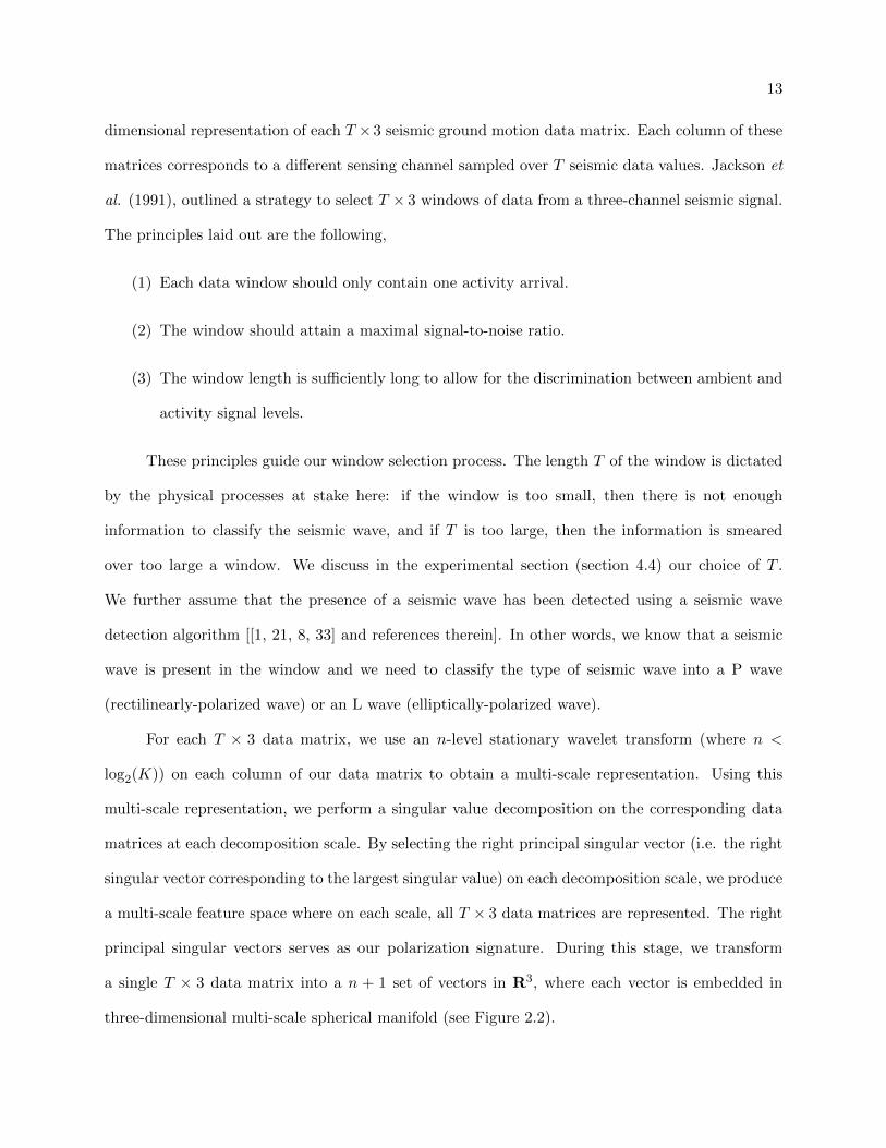
13

dimensional representation of each T ×3 seismic ground motion data matrix. Each column of these

matrices corresponds to a different sensing channel sampled over T seismic data values. Jackson et

al. (1991), outlined a strategy to select T × 3 windows of data from a three-channel seismic signal.

The principles laid out are the following,

(1) Each data window should only contain one activity arrival.

(2) The window should attain a maximal signal-to-noise ratio.

(3) The window length is sufficiently long to allow for the discrimination between ambient and

activity signal levels.

These principles guide our window selection process. The length T of the window is dictated

by the physical processes at stake here: if the window is too small, then there is not enough

information to classify the seismic wave, and if T is too large, then the information is smeared

over too large a window. We discuss in the experimental section (section 4.4) our choice of T .

We further assume that the presence of a seismic wave has been detected using a seismic wave

detection algorithm [[1, 21, 8, 33] and references therein]. In other words, we know that a seismic

wave is present in the window and we need to classify the type of seismic wave into a P wave

(rectilinearly-polarized wave) or an L wave (elliptically-polarized wave).

For each T × 3 data matrix, we use an n-level stationary wavelet transform (where n <

log2(K)) on each column of our data matrix to obtain a multi-scale representation. Using this

multi-scale representation, we perform a singular value decomposition on the corresponding data

matrices at each decomposition scale. By selecting the right principal singular vector (i.e. the right

singular vector corresponding to the largest singular value) on each decomposition scale, we produce

a multi-scale feature space where on each scale, all T × 3 data matrices are represented. The right

principal singular vectors serves as our polarization signature. During this stage, we transform

a single T × 3 data matrix into a n + 1 set of vectors in R3, where each vector is embedded in

three-dimensional multi-scale spherical manifold (see Figure 2.2).

14

In the supervised phase learning stage of our algorithm, we use a database of labeled phases

to classify seismic data for which the phase is unknown. We accomplish this by using machine

learning techniques on each spherical feature manifold where both the testing and training data

reside. By merging the classification results from our multi-scale feature manifolds, we are able to

produce a classification result for each unlabeled T × 3 data matrix. Figure 1.7 is a block diagram

of our algorithm.

1.5 Scope and Overview

This thesis is organized in the following way:

• Chapter 2 reviews both the classical approach and our approach to polarization analysis.

We present methods which extract polarization features using the time-domain signals and

spectral decomposition thereof. This chapter represents one major contribution of our

work, in that it presents an alternative view of the polarization feature vector.

• Chapter 3 presents our classification framework. We discuss a concept from machine learn-

ing called Supervised Learning and describe algorithms under this paradigm. We also

present the second major contribution of our work, the notion of lifting these machine

learning algorithms to the spherical polarization feature space.

• Chapter 4 shows experimental results for both a classical phase labeling method and our

supervised learning approach. We discuss our algorithms performance and the choice of

system parameters.

• Chapter 5 provides a discussion of our methods and future directions for research in this

area.

Chapter 2

Feature Extraction

Given a data set one may find it more beneficial to work with a transformed version of that

data. In these cases, we refer to measures derived from the data as features. Features are useful for

casting the data from a different perspective and ensuring that what is being analyzed is described

by only its most pertinent components. One example of the utility of extracting features from

data comes from the analysis of musical genres. In this case, the data set is made up of segments

from musical soundtracks coming form different musical genres such as rock, classical, electronic,

hip-hop, etc. The goal may be to take a musical soundtrack for which the genre is not known and

determine in which genre it best “fits”. Instead of working with the musical time series, it is more

beneficial to work with features that describe the track, such as timber, tempo, frequency content,

and zero crossings, to name a few. By transforming the data it is in some cases easier to understand

structures in the data that lead to better classification results.

In this chapter, we discuss both standard phase estimation methods and our approach for

extracting phase features across multiple frequency bands that reside on the three dimensional

sphere.

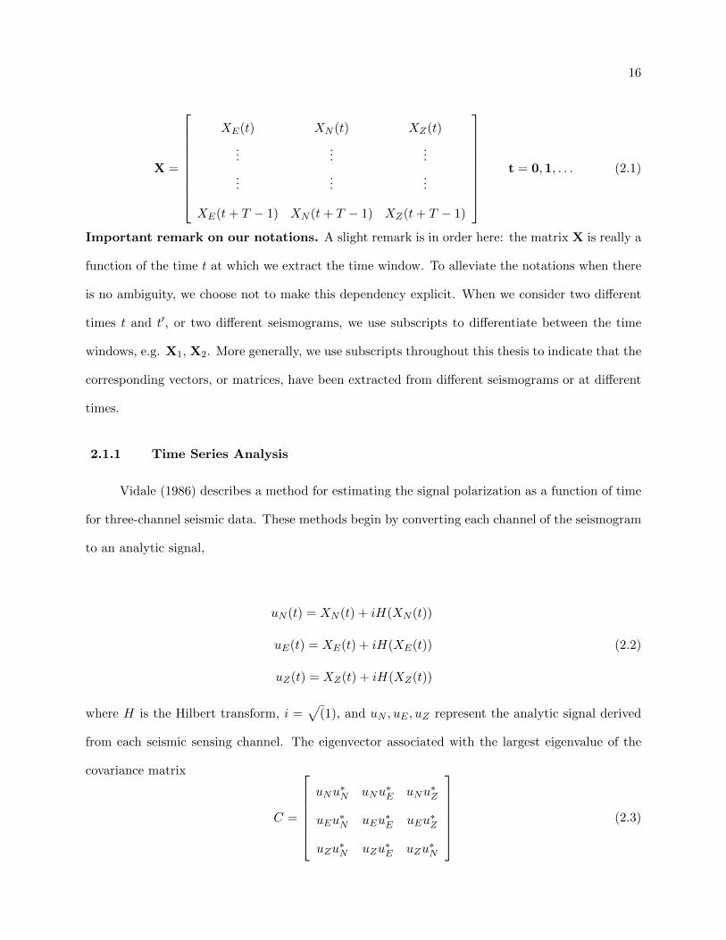
2.1 Phase Estimation Methods

Our analysis of the seismogram is performed on a sliding time windows of the three component

seismogram [XE(t) XN (t) XZ(t)]T , t = 0, 1, . . . (see Fig. 1). We form the matrix X by collecting

T samples of the seismogram and stacking them into a T × 3 matrix

16

X =

XE(t) XN (t) XZ(t)

......

...

......

...

XE(t+ T − 1) XN (t+ T − 1) XZ(t+ T − 1)

t = 0,1, . . . (2.1)

Important remark on our notations. A slight remark is in order here: the matrix X is really a

function of the time t at which we extract the time window. To alleviate the notations when there

is no ambiguity, we choose not to make this dependency explicit. When we consider two different

times t and t′, or two different seismograms, we use subscripts to differentiate between the time

windows, e.g. X1, X2. More generally, we use subscripts throughout this thesis to indicate that the

corresponding vectors, or matrices, have been extracted from different seismograms or at different

times.

2.1.1 Time Series Analysis

Vidale (1986) describes a method for estimating the signal polarization as a function of time

for three-channel seismic data. These methods begin by converting each channel of the seismogram

to an analytic signal,

uN (t) = XN (t) + iH(XN (t))

uE(t) = XE(t) + iH(XE(t)) (2.2)

uZ(t) = XZ(t) + iH(XZ(t))

where H is the Hilbert transform, i =√

(1), and uN , uE , uZ represent the analytic signal derived

from each seismic sensing channel. The eigenvector associated with the largest eigenvalue of the

covariance matrix

C =

uNu

∗N uNu

∗E uNu

∗Z

uEu∗N uEu

∗E uEu

∗Z

uZu∗N uZu

∗E uZu

∗N

(2.3)

17

points in the direction of the greatest amount of polarization. Computing the degree of polarization

begins by rotating this eigenvector such that the real component is maximized. The maximal real

component may be found by computing,

V = max0<α<180

√Re (x0cis(α))2 +Re (y0cis(α))2 +Re (z0cis(α))2 (2.4)

where cis(α) = cos(α) + i sin(α) and α is the rotation. The degree of polarization is given by,

P (t) =

√1− V 2

V. (2.5)

If P (t) is near unity, then the motion at time t is said to be circularly polarized. However, if P (t)

is near zero, then the motion is called linearly polarized. This method gives three-channel signal

polarization as a function of time.

Jackson et al. (1991) proposed a statistical test (F-test) for classifying seismic waves. The

authors estimated the polarization of the seismic wave from the singular value decomposition of

the raw seismic data X, see equation 2.1,

X = UΣV T . (2.6)

The matrix Σ is a 3 × 3 diagonal matrix that contains the singular values, σ1 ≥ σ2 ≥ σ3. Under

the assumption that there is only a linearly polarized wave within X, then the noise energy, not

captured by the main singular vector, is given by σ21 + σ22 +σ22+σ

23

2 . Similarly, if the seismic wave

is elliptically polarized, then the noise energy is given by 3(σ23). As a result, the ratio of the noise

energies,

F =σ21 + σ22 +

σ22+σ

23

2

3(σ23), (2.7)

can be used to differentiate between the two types of polarization. The authors then proposed

to test the null hypothesis H0: the wave captured in the window X is linearly polarized

against the alternative hypothesis H1: the wave captured in the window X is elliptically

polarized. The significance level of the test is given by

Ψ nn+nF

(n

2,n

2) =

1

β(n2 ,n2 )

∫ nn+nF

0tn2−1(1− t)

n2−1dt, (2.8)

18

where Ψ is the incomplete beta function. The number n is an estimate of the number of independent

samples in the signal window X and β is the standard beta function. The number of independent

samples n is determined by counting the number of peaks present in the Fourier transform of X.

Additional technical details can be found in the original paper [15].

2.1.2 Spectral Methods

The concept of signal polarization as a function of frequency was presented by Park (1986).

In this work, his analysis began by applying the Short Time Discrete Fourier Transform to each

channel of the three-channel seismogram, X, and anlyzing the eigenspectra of the resulting spectral

matrix M(f) given by,

M(f) =

y10(f) y20(f) y30(f)

......

...

......

...

y1K−1(f) y2K−1(f) y3K−1(f)

(2.9)

where K is the number of spectral components and yj(f) is given by,

yk(f) =1

Nτ

N−1∑n=0

wnxk(nτ)ei2πfnτ k = 1, 2, 3 (2.10)

where τ is the sampling interval, Nτ is the length of the time series, and {wn}N−1n=0 is a window

function. He proposed to estimate the dominant direction of polarization by using the principal

singular vector in the SVD of M(f).

An issue that results by taking this approach is that the Fourier basis is not the most well-

suited basis to represent seismic signals. Seismological signal are short-lived signals that result from

bursts of energy. A Fourier Transform of this type of signal will result in an expansion with many

Fourier coefficients due to fitting sharp signal transitions. A better suited basis is the wavelet basis

because it is better able to represent sharp transitions with fewer coefficients.

19

Auria et al. (2010) proposed the use of the Wavelet Transform to decompose each channel of

the three-channel seismogram and subsequently analyze the direction of dominant polarization at

the level of the signal scale. As presented in Kumar and Foufoula-Georgiou (1997), the orthogonal

Discrete Wavelet Transform (DWT) of a time series x(tk) is given by,

x(tk) =∑m

∑n

cm,nψm,n(tk) (2.11)

where ψm,n(tk) is defined as

ψm,n(tk) =1√2m

ψ

(t− n2m

2m

). (2.12)

Here, ψ is called the mother wavelet. The DWT coefficients can be computed by,

cm,n =∑m

∑n

x(tk)ψm,n(tk) (2.13)

Auria et al. proposed to use the DWT of each channel of the three-channel seismogram and its

corresponding Hilbert transform to estimate polarization. For each seismogram channel,XN (t), XE(t),

and XZ(t) they computed,

θm,nN = cm,nN + iH(cm,nN )

θm,nE = cm,nE + iH(cm,nE ) (2.14)

θm,nZ = cm,nZ + iH(cm,nZ )

In a similar way to frequency domain polarization analysis, they computed a covariance matrix for

each triplet of complex coefficients θm,n

Θm,nkj = θm,nk θm,nj . (2.15)

By computing the SVD of this matrix and applying methods developed by Vidale (1986), they

estimated the degree of polarization using equation 2.5. This process provides an estimate of the

20

polarization across multiple levels of signal scale as a function of time.

These methods share the common theme of estimating the direction of dominant polarization

and then computing the degree of polarization in some fashion. We propose to use the geometric

description of the direction of dominant polarization over a window of seismic data as a function of

signal frequency band. This description is used as the discriminating factor in polarization analysis.

In the next section, we explore this concept further.

2.2 Geometric Polarization Analysis

In our quest to characterize the polarization content in the time window X, recall equation

2.1, we propose to decompose the seismic waveform X into a series of components that characterize

the Earth motion at multiple scales. For each scale, we extract the main direction of the Earth

motion at that scale and use this information as the input to a classifier. In this section, we describe

the multi-scale analysis of the matrix X and reserve the discussion on classification for Chapter 3.

We decompose each of the three columns of X with a redundant l-level stationary wavelet

transform (where l ≤ log2(T )). The stationary wavelet decomposition is a redundant transform:

we obtain l × T coefficients for each of the three directions of the seismogram. Fortunately, there

exists a fast algorithm to compute the stationary wavelet decomposition: the “a trou” algorithm

[27].

Figure 2.1 shows a seismic signal (top left), its corresponding spectrogram (bottom left),

and the stationary wavelet transform coefficients (right). The stationary wavelet transform is able

to detect the second and third seismic waves, whereas the spectrogram hardly changes when the

waves arrive (see Fig. 2.1-bottom left). Because seismograms can be approximated with very high

precision using a small number of wavelet coefficients ([3, 17, 25, 39, 9], and refrences therein), the

wavelet transform is better suited than a short-time Fourier transform to detect seismic waves of

small amplitude, as shown in this example.

21

10 20 30 40 50 60 70 80 90 100−3

−2

−1

0

1

2

3x 10

5

time (s)

Am

plitu

de

10 20 30 40 50 60 70 80 90 1000

5

10

15

20

time (s)

freq

(H

z)

time (s)

Sca

le 2−

j

10 20 30 40 50 60 70 80 90 100

1

2

3

4

5

6

7

8

9 −1.5

−1

−0.5

0

0.5

Figure 2.1: Left: Z channel of a seismic signal (top) and spectrogram (bottom). The arrival times

of three seismic waves are marked by vertical bars. Note that the second and third waves hardly

elicit any changes in the spectrogram. Right: stationary wavelet transform of the waveform shown

in left. The magnitude is color coded and displayed as a function of time, from fine scale (top) to

coarse scale (bottom).

The outcome of the stationary wavelet analysis of X at scale j can be represented as a T × 3

matrix Wj given by

Wj =

W jE(0) W j

N (0) W jZ(0)

......

...

......

...

......

...

W jE(T − 1) W j

N (T − 1) W jZ(T − 1)

j = 1, . . . , l, (2.16)

where each column is the stationary wavelet transform of the corresponding column in X. In

practice, we choose l to be the maximum scale allowed by the size of the signal (T ) and the size

of the filter. The matrix Wj encodes the motion of the Earth – measured between time t and

(t+ T − 1) – in all three directions at scale j .

In order to find the direction associated with the main energy at scale j, we compute the

22

singular value decomposition of Wj ,

Wj =

Uj,1 Uj,2 Uj,3

σj,1 0 0

0 σj,2 0

0 0 σj,3

[Vj,1]T

[Vj,2]T

[Vj,3]T

(2.17)

where σj,1 ≥ σj,2 ≥ σj,3, and ‖Uj,i‖ = ‖Vj,i‖ = 1, i = 1, 2, 3. Furthermore, the T -dimensional

vectors Uj,1,Uj,2 and Uj,3 are orthogonal, and the 3-dimensional vectors Vj,1,Vj,2 and Vj,3 are

also orthogonal. The vector Vj,1 is known as the polarization vector in the seismic literature. At

each scale j, we only retain Vj,1 (and we discard all the remaining vectors), and we denote it by

νj ,

νj = Vj,1. (2.18)

In summary, we map the T × 3 matrix X to the 3× l multiscale polarization matrix given by,

X 7→[ν1 · · · · · · νl

]. (2.19)

This map extracts the direction of maximal polarization over multiple frequency bands. Essentially,

it is a filtering of the polarization vectors over different regions in the frequency spectrum. The

wavelet filter used is also important and depending on the filter the quality of the polarization

filtering will vary. Indeed, wavelet filters that are orthogonal, and subsequently have linear-phase,

are expected to perform better than non-orthogonal wavelets. Figure 2.2 shows feature extraction

results.

23

Figure 2.2: Left: stationary wavelet transform for several Xi, i = 1, . . . superimposed on top of one

another; top two rows: scaling function (W1), middle two rows: coarsest (largest scale) wavelet

(W2), bottom two rows: next finer scale wavelet (W3). Right: the vectors νji are represented

as points on the sphere; each row corresponds to the same scale j as the two plots on the left

(j = 1, 2, 3 from top to bottom). The color and shape of νj encode the type of wave: red star for

P, blue cross for L, and green circles for testing data.

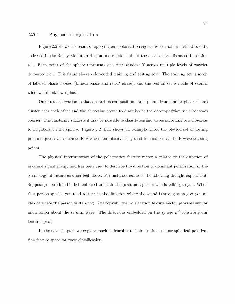
24

2.2.1 Physical Interpretation

Figure 2.2 shows the result of applying our polarization signature extraction method to data

collected in the Rocky Mountain Region, more details about the data set are discussed in section

4.1. Each point of the sphere represents one time window X across multiple levels of wavelet

decomposition. This figure shows color-coded training and testing sets. The training set is made

of labeled phase classes, (blue-L phase and red-P phase), and the testing set is made of seismic

windows of unknown phase.

Our first observation is that on each decomposition scale, points from similar phase classes

cluster near each other and the clustering seems to diminish as the decomposition scale becomes

coarser. The clustering suggests it may be possible to classify seismic waves according to a closeness

to neighbors on the sphere. Figure 2.2 -Left shows an example where the plotted set of testing

points in green which are truly P-waves and observe they tend to cluster near the P-wave training

points.

The physical interpretation of the polarization feature vector is related to the direction of

maximal signal energy and has been used to describe the direction of dominant polarization in the

seismology literature as described above. For instance, consider the following thought experiment.

Suppose you are blindfolded and need to locate the position a person who is talking to you. When

that person speaks, you tend to turn in the direction where the sound is strongest to give you an

idea of where the person is standing. Analogously, the polarization feature vector provides similar

information about the seismic wave. The directions embedded on the sphere S2 constitute our

feature space.

In the next chapter, we explore machine learning techniques that use our spherical polariza-

tion feature space for wave classification.

Chapter 3

Seismic Phase Learning

3.1 Supervised Learning

“Learning is defined as acquiring new or modifying existing knowledge, behaviors, skills,

values, or preferences and may involve synthesizing different types of information” [37]. Machine

Learning attempts to learn patterns and regularities in data. A popular example is that of rec-

ommendation systems, which attempt to provide suggestions based on previous experiences. For

instance, when users provide feedback, in terms of likes and dislikes of a song, on internet radio

sites, recommendation systems can take these inputs to suggest new songs that may be appealing to

the user. The process of extracting information from the data provided and performing operations

with the information found summarizes the basis of machine learning.

More specifically, there is a class of machine learning tasks that learns from data that has

been fully labeled. This is known as supervised machine learning, or supervised learning. This

methodology will be the focus of this chapter and will be presented from the perspective of learning

the phase of an unlabeled seismic wave.

3.1.1 Supervised learning for Phase Classification

In our setting, we wish to learn the phase for a seismic wave captured in the time window X

from existing labeled examples. The labeled examples are obtained from seismic activity recorded

at different stations within a regional sensing network that has been pre-analyzed by an expert

analyst.

26

By extracting information from the time window X through the process of feature extraction

and observing the natural clustering in the feature space, we are able to take advantage of supervised

learning techniques. The successfulness of these techniques are directly related to the structure

inherent in the feature space. If the feature extraction methods yield poor structure, then the

methods for learning something about an unlabeled example cannot be expected to be accurate.

The first step to good supervised learning is good feature engineering.

In our setting, we are given a time window X within which we have detected a seismic

wave. Our goal is to classify the wave as being a body wave (P) or a surface wave (L) based on the

information provided by the vectors {ν1, . . . , νl}. Our proposal is to decouple the scales j = 1, . . . , l

and perform the classification of each vector νj independently. In order to classify νj , we will think

of νj as a point on the two-dimensional unit sphere S2 in R3 (‖νj‖ = 1). Thus, we are facing the

problem of binary classification on the sphere: does νj belong to the class of P waves, or does it

belong to the class of L waves?

3.2 Classifiers

We assume that our training set is composed of N time windows Xi, i = 1, . . . , N , for which

we know the labels

yi =

1 if the time window Xi contains a P wave,

−1 if the time window Xi contains an L wave.

From each Xi, we compute the l singular vectors ν1i ,..,νli . Our goal is to construct at each scale

j a function f j that maps a testing point νj , with an unknown label, from the sphere S2 to the

interval [−1, 1],

f j : νj ∈ S2 7→ f j(νj) ∈ [−1, 1].

We evaluated three different classification methods (three different types of f j) using the

kernel described in section 3.3.1: kernel ridge regression, kernel support vector machines, and k-

nearest neighbors. We use the same type of classification method f j for all the scales j = 1, . . . , l.

27

Only the parameters of each function f j vary across the scales. In the following sections, we describe

the three different approaches. Additional details about the implementations of these techniques

can be found in ([13, 14] and references therein).

3.2.1 Kernel Support Vector Machines

The support vector machine (SVM) is one of the most popular machine learning techniques

available. When the data is linearly separable, the SVM attempts to find the optimal separating

hyperplane. In addition, the SVM can be applied to data not linearly separable by using the “kernel

trick” to inject the data into a higher dimensional space where the data may be separated by a

hyperplane. Figure 3.1 shows a graphical description of both cases. In our case, we are attempting

to locally learn the boundaries between different seismic phase classes distributed over the feature

space.

W

supportvectors

margin|W| ||2

������

������

������

������

������

������ ��

������

��������

��������

��������

������

������

���

���

���

���

��������

������

������

��������

������

������

���

���

������

������

��������

������

������

������

������

���

���

��������

��������

������

������

��������

��������

��������

������

������

������

������

������

������

������

������

��������

��������

��������

1

2X

Xi

X������

������

��������

������

������

������

������

������

������

������

������

������

������

��������

������

������

��������

��������

������

������

������

������

������

������

������

������

��������

������

������

������

������

��������

��������

������������

������

������

������

������

��������

��������

������

������

������

������

��������

��������

��������

������

������

��������

��������

��������

��������

���

���

��������

��������

������

������

������

������

��������

��������

������

������

������

������

��������

��������

������

������

��������

��������

��������

��������

������

������

���

���

���

���

������

������

������

������

������

������

��������

������

������

������

������

������

������

������

������

��������

Xi

X

2

1

X

Figure 3.1: Left: Maximum margin SVM diagram. Right: Kernel Trick. Copied from [4] without

permission.

28

The SVM classification function f j is given by

f j(νj) = sgn

(N∑i=1

λji yji κ(νj , νji ) + bj

), (3.1)

where the λji are found by solving the dual form of the optimization problem,

maximizeλji

N∑i=1

λji −1

2

N∑i=1

N∑i′=1

λji yji λ

ji′ y

ji′ κ(νji , ν

ji′),

subject to λji ≥ 0, i = 1, . . . , N andN∑i=1

yjiλji = 0.

(3.2)

The constant bj is given by

bj = mean

{(

N∑i=1

λjiyji κ(νjk, ν

ji )− ck), k = 1, . . . , N, such that λjk > 0

}. (3.3)

3.2.2 Kernel Ridge Regression

In ridge regression, we attempt to find a linear function that models the dependencies between

the input variables {νji } and the response variables {yji }. The ridge component attempts to delineate

the boundary between classes of input variables. The kernelized version of this approach allows us

to measure distances in some feature space other than the standard Euclidean space. In our case,

we are learning the correspondence between the locations in the feature space to the class of the

corresponding seismic phases.

The kernel ridge regression function f j is given by

f j(νj) =N∑i=1

βji κ(νj , νji ), (3.4)

where the kernel κ is defined by (3.9), and the coefficients {βj1, · · · , βjN} are estimated from the

training points by solving the optimization problem [13],

minβj‖yj − βjΞj‖22 + λ‖βj‖22, (3.5)

where yj = [yj1, · · · , yjN ]t, βj = [βj1, · · · , β

jN ], ϕjn = 1

N

∑Ni=1 κ(νjn, ν

ji ), and

Ξj =

κ(νj1, ν

j1)− ϕj1 · · · κ(νjN , ν

j1)− ϕjN

......

κ(νj1, νjN )− ϕj1 · · · κ(νjN , ν

jN )− ϕjN

. (3.6)

29

The unique solution [13] to the above optimization problem is given by

β∗j =(ΞjTΞj − λI

)−1ΞjTyj ,

where I is the N ×N identity matrix.

3.2.2.1 Regularization Parameter

The regularization parameter λ serves two tasks. Primarily, λ ensures that the inverse exists

by forcing the eigenvalues of(ΞjTΞj − λI

)to be bounded away from zero. Secondly, we can

interpret the regularization parameter as controlling the stiffness of the boundary between classes

of input variables. When λ is small, the stiffness is low. On the other hand, a large λ represents a

high stiffness boundary. Figure 3.2 shows a representation of this concept.

Figure 3.2: Illustration of the stiffness interpretation of the regularization parameter λ. Dashed

line represents a low stiffness value and the solid line represents a high stiffness line. Copied form

[4] without permission.

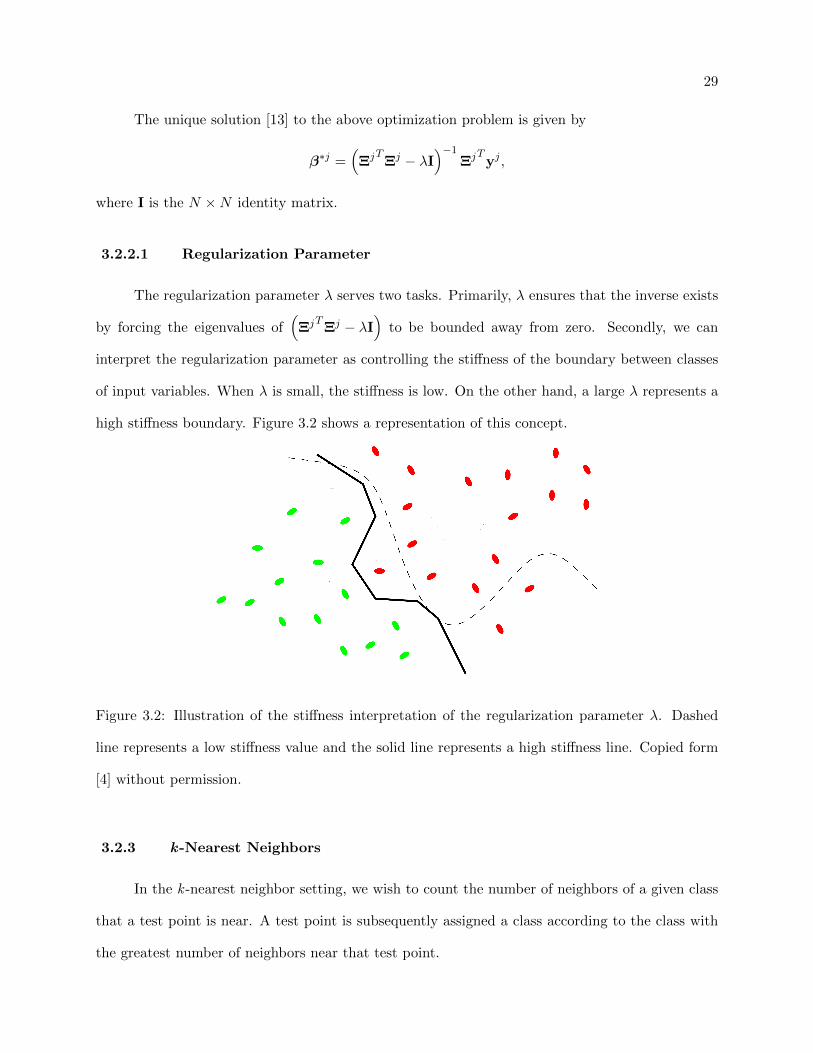
3.2.3 k-Nearest Neighbors

In the k -nearest neighbor setting, we wish to count the number of neighbors of a given class

that a test point is near. A test point is subsequently assigned a class according to the class with

the greatest number of neighbors near that test point.

30

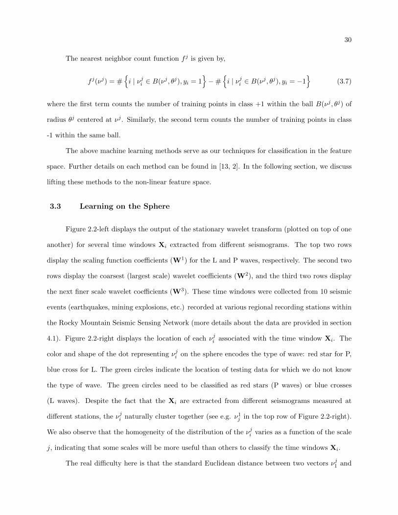
The nearest neighbor count function f j is given by,

f j(νj) = #{i | νji ∈ B(νj , θj), yi = 1

}−#

{i | νji ∈ B(νj , θj), yi = −1

}(3.7)

where the first term counts the number of training points in class +1 within the ball B(νj , θj) of

radius θj centered at νj . Similarly, the second term counts the number of training points in class

-1 within the same ball.

The above machine learning methods serve as our techniques for classification in the feature

space. Further details on each method can be found in [13, 2]. In the following section, we discuss

lifting these methods to the non-linear feature space.

3.3 Learning on the Sphere

Figure 2.2-left displays the output of the stationary wavelet transform (plotted on top of one

another) for several time windows Xi extracted from different seismograms. The top two rows

display the scaling function coefficients (W1) for the L and P waves, respectively. The second two

rows display the coarsest (largest scale) wavelet coefficients (W2), and the third two rows display

the next finer scale wavelet coefficients (W3). These time windows were collected from 10 seismic

events (earthquakes, mining explosions, etc.) recorded at various regional recording stations within

the Rocky Mountain Seismic Sensing Network (more details about the data are provided in section

4.1). Figure 2.2-right displays the location of each νji associated with the time window Xi. The

color and shape of the dot representing νji on the sphere encodes the type of wave: red star for P,

blue cross for L. The green circles indicate the location of testing data for which we do not know

the type of wave. The green circles need to be classified as red stars (P waves) or blue crosses

(L waves). Despite the fact that the Xi are extracted from different seismograms measured at

different stations, the νji naturally cluster together (see e.g. ν1j in the top row of Figure 2.2-right).

We also observe that the homogeneity of the distribution of the νji varies as a function of the scale

j, indicating that some scales will be more useful than others to classify the time windows Xi.

The real difficulty here is that the standard Euclidean distance between two vectors νj1 and

31

νj2, originating from two different time windows X1 and X2, is meaningless in this context. In the

case where points are sampled from a surface, or more generally a manifold, we need to measure

distances using the geodesic distance defined on the manifold. Alternatively, we can construct

an embedding of the manifold into Rm that optimally preserves distances (e.g. bi-Lipschitz), and

measure distances in Rm.

In our case, we have access to a closed-form expression for the geodesic distance and are

therefore able to account for the nonlinear structure of the feature space to classify the vectors νji .

We note that when the true geodesic distance is not accessible, an approximation to the geodesic

distance is usually close to optimal. For instance, Turaga et al. (2008) showed that the Procrustes

approximations to the geodesic distance on the Stiefel and Grassmann manifolds yield results that

are close to optimal for various problems involving the estimation of model parameters in dynamical

systems, activity recognition, and video-based face recognition [35]. However, the computation of

the geodesic distance may prove to be very expensive. Sommer et al. (2010) showed that the gain

in accuracy achieved with the true geodesic did not outweigh the computation cost when the exact

geodesic was compared to a linear approximation in the context of Principal Geodesic Analysis

[28].

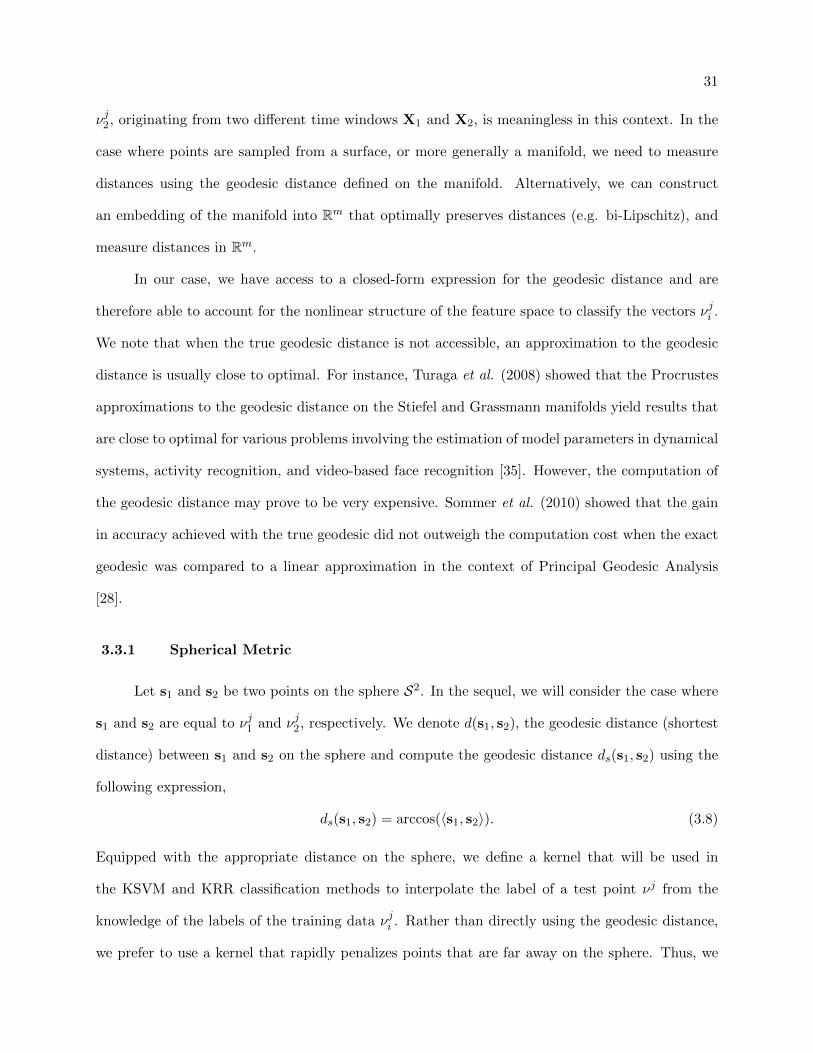
3.3.1 Spherical Metric

Let s1 and s2 be two points on the sphere S2. In the sequel, we will consider the case where

s1 and s2 are equal to νj1 and νj2, respectively. We denote d(s1, s2), the geodesic distance (shortest

distance) between s1 and s2 on the sphere and compute the geodesic distance ds(s1, s2) using the

following expression,

ds(s1, s2) = arccos(〈s1, s2〉). (3.8)

Equipped with the appropriate distance on the sphere, we define a kernel that will be used in

the KSVM and KRR classification methods to interpolate the label of a test point νj from the

knowledge of the labels of the training data νji . Rather than directly using the geodesic distance,

we prefer to use a kernel that rapidly penalizes points that are far away on the sphere. Thus, we

32

introduce two nonlinearities in the following way,

κ(s1, s2) = exp

(− ds(s1, s2)

σ (π − ds(s1, s2))

). (3.9)

The presence of the denominator in the argument of the exponential enforces arbitrarily small

distance between points that are polar opposites on the sphere. A scaling factor σ is adjusted

according to the sampling density (see discussion in section 4.4 for more details on the choice of

σ). The following section discuss our classification procedure.

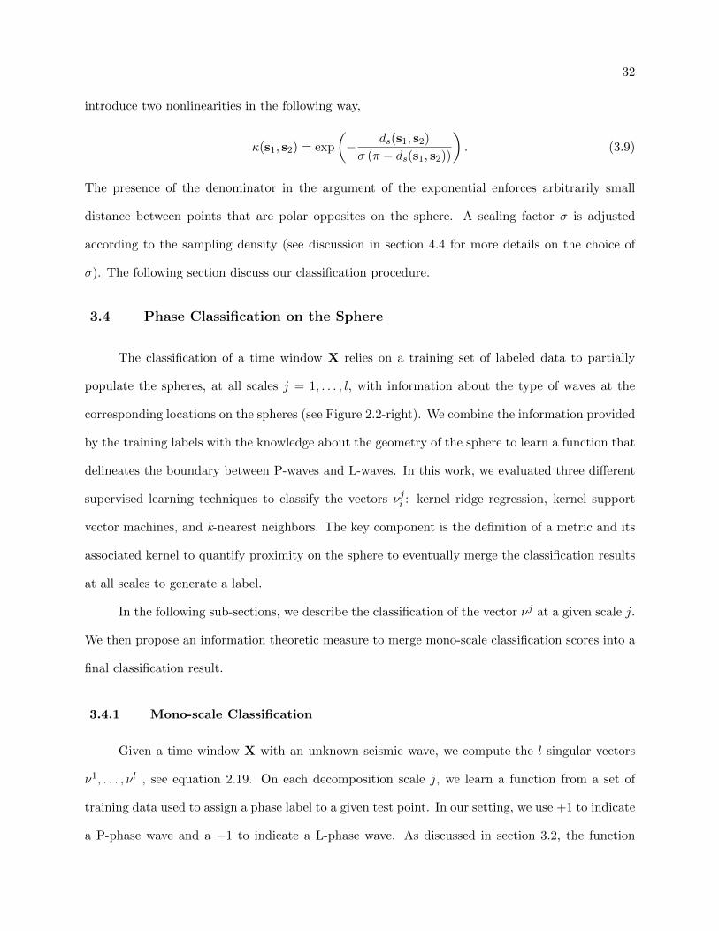
3.4 Phase Classification on the Sphere

The classification of a time window X relies on a training set of labeled data to partially

populate the spheres, at all scales j = 1, . . . , l, with information about the type of waves at the

corresponding locations on the spheres (see Figure 2.2-right). We combine the information provided

by the training labels with the knowledge about the geometry of the sphere to learn a function that

delineates the boundary between P-waves and L-waves. In this work, we evaluated three different

supervised learning techniques to classify the vectors νji : kernel ridge regression, kernel support

vector machines, and k-nearest neighbors. The key component is the definition of a metric and its

associated kernel to quantify proximity on the sphere to eventually merge the classification results

at all scales to generate a label.

In the following sub-sections, we describe the classification of the vector νj at a given scale j.

We then propose an information theoretic measure to merge mono-scale classification scores into a

final classification result.

3.4.1 Mono-scale Classification

Given a time window X with an unknown seismic wave, we compute the l singular vectors

ν1, . . . , νl , see equation 2.19. On each decomposition scale j, we learn a function from a set of

training data used to assign a phase label to a given test point. In our setting, we use +1 to indicate

a P-phase wave and a −1 to indicate a L-phase wave. As discussed in section 3.2, the function

33

learned on scale j is given by f j(νj).

On the decomposition scale j, the unlabeled feature vector νj is assigned a phase class

according to the following rule,

P wave if f j(νj) > 0,

L wave if f j(νj) < 0,

No Solution if f j(νj) = 0.

(3.10)

A situation may arise when a test point is near an equal number of training points from each

class. In this case, the classification may become unresolvable. To help understand the homogeneity

of the training points near the test point, we employ an information theoretic measure to help

identify areas of low and high classification confidence.

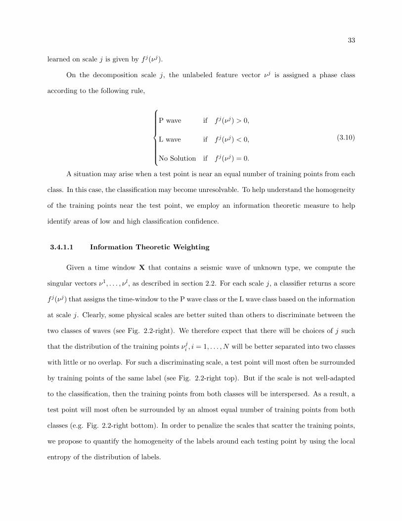
3.4.1.1 Information Theoretic Weighting

Given a time window X that contains a seismic wave of unknown type, we compute the

singular vectors ν1, . . . , νl, as described in section 2.2. For each scale j, a classifier returns a score

f j(νj) that assigns the time-window to the P wave class or the L wave class based on the information

at scale j. Clearly, some physical scales are better suited than others to discriminate between the

two classes of waves (see Fig. 2.2-right). We therefore expect that there will be choices of j such

that the distribution of the training points νji , i = 1, . . . , N will be better separated into two classes

with little or no overlap. For such a discriminating scale, a test point will most often be surrounded

by training points of the same label (see Fig. 2.2-right top). But if the scale is not well-adapted

to the classification, then the training points from both classes will be interspersed. As a result, a

test point will most often be surrounded by an almost equal number of training points from both

classes (e.g. Fig. 2.2-right bottom). In order to penalize the scales that scatter the training points,

we propose to quantify the homogeneity of the labels around each testing point by using the local

entropy of the distribution of labels.

34

Figure 3.3: Example of two test points νj1 and νj2 in green. The point on the left has a low local

entropy and therefore, a higher confidence in correct classification. The test point on the right has

a high local entropy and thus a low confidence in correct classification.

Given a scale j, we define the entropy of the distribution of labels yi within the ball B(s, θ) of

radius θ centered at s as follows,

hj(s) = −P j+1(s) log2 Pj+1(s)− P j−1(s) log2 P

j−1(s), (3.11)

where P j+1(s) and P j−1(s) are the probabilities that the label of a random training point inside the

ball B(s, θ) be a +1 or −1 respectively,

P j+1(s)) = Pr[νji ∈ B(s), θ) ∩ yi = 1

]and P j−1(s)) = Pr

[νji ∈ B(s), θ) ∩ yi = −1

]. (3.12)

It is useful to examine the two extreme cases: hj(s) = 0 and hj(s) = 1. If P j+1(s) = 0 or

P j−1(s) = 0, then the ball B(s, θ) is centered in a region of the sphere where the distribution of labels

is uniform. This is the most favorable case since the testing point s can reliably use the labels of

the local training points. The other extreme corresponds to the case where P j+1(s) = P j−1(s) = 1/2.

In this case, the training data are useless since there are as many P waves as there are L waves

inside the ball. The label returned by the classifier f j(s) should not be used. Figure 3.3 displays

these two situations: the testing point νj1 on the left of the sphere is surrounded by almost only L

35

waves, and therefore hj(νj1) will be close to 0. On the right side, the testing point νj2 appear to be

encircled by an equal number of L and P waves, and therefore we expect that hj(νj2) ≈ 1.

We propose to use 1−hj(s) as a measure of the quality of the label returned by the classifier

f j(s) at scale j. In rare cases, a testing point νj might be uniformly surrounded by training points

from the opposite class. In such a case, the calculated entropy would be misleading with respect

to the correct label. As a result, one must consider all scales in order to resolve such issues.

3.4.2 Multi-Scale Classification

For each νj , a classifier at scale j returns a label f j(νj) and a measure of the quality of the

label, 1− hj(νj). We combine these results to form the estimate of the label given by

P wave if∑l

j=1[1− hj(νj)]f j(νj) > 0,

L wave if∑l

j=1[1− hj(νj)]f j(νj) < 0,

No Solution if∑l

j=1[1− hj(νj)]f j(νj) = 0.

(3.13)

With the classification methods in hand, the next chapter describes our data set, testing

methodology, and classification results.

Chapter 4

Experimental Results

4.1 Data

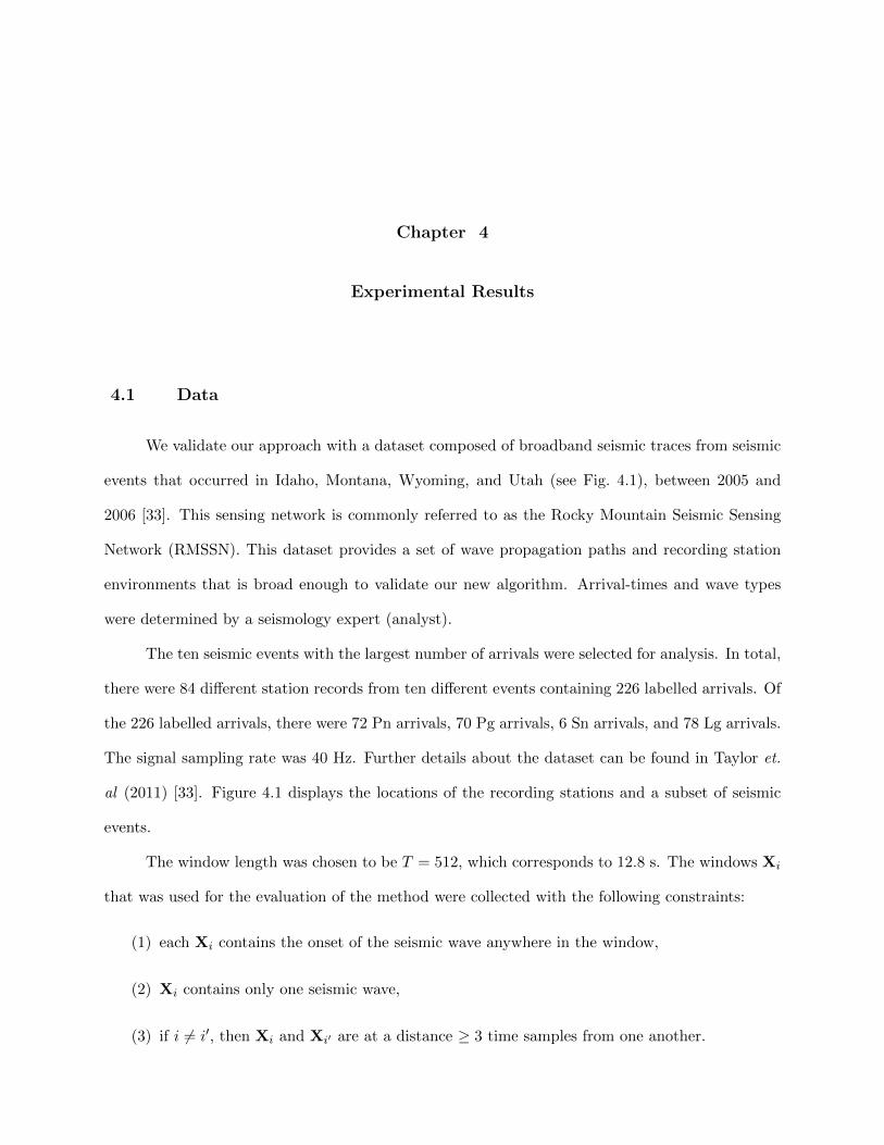
We validate our approach with a dataset composed of broadband seismic traces from seismic

events that occurred in Idaho, Montana, Wyoming, and Utah (see Fig. 4.1), between 2005 and

2006 [33]. This sensing network is commonly referred to as the Rocky Mountain Seismic Sensing

Network (RMSSN). This dataset provides a set of wave propagation paths and recording station

environments that is broad enough to validate our new algorithm. Arrival-times and wave types

were determined by a seismology expert (analyst).

The ten seismic events with the largest number of arrivals were selected for analysis. In total,

there were 84 different station records from ten different events containing 226 labelled arrivals. Of

the 226 labelled arrivals, there were 72 Pn arrivals, 70 Pg arrivals, 6 Sn arrivals, and 78 Lg arrivals.

The signal sampling rate was 40 Hz. Further details about the dataset can be found in Taylor et.

al (2011) [33]. Figure 4.1 displays the locations of the recording stations and a subset of seismic

events.

The window length was chosen to be T = 512, which corresponds to 12.8 s. The windows Xi

that was used for the evaluation of the method were collected with the following constraints:

(1) each Xi contains the onset of the seismic wave anywhere in the window,

(2) Xi contains only one seismic wave,

(3) if i 6= i′, then Xi and Xi′ are at a distance ≥ 3 time samples from one another.

37

Figure 4.1: Map of Rocky Mountain Seismic Sensing Network

0.5 1 1.5 2 2.5 3 3.5 4

x 104

−5

0

5

x 104

BH

Z

0.5 1 1.5 2 2.5 3 3.5 4

x 104

−5

0

5

x 104

BH

N

0.5 1 1.5 2 2.5 3 3.5 4

x 104

−5

0

5

10x 10

4

i

BH

E

Pn−phase

Pg−phase Lg−phase

Figure 4.2: Seismogram captured at “Elk” station in the sensing network. Vertical bars representpredetermined arrival times. The seismic phase has been annotated for each event. The particulararrivals on each channel correspond to the same phase.

38

All algorithms were developed using Matlab r computational software. In the following sections,

we discuss our preprocessing of the seismic data, our evaluation strategy, the techniques we use for

classifier parameter estimation, and provide our experimental results.

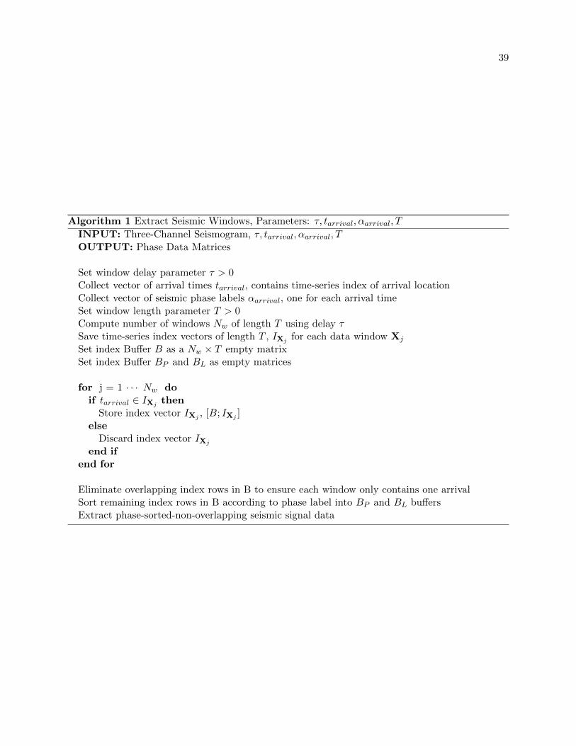
4.2 Preprocessing

Figure 4.1 shows an example of a typical three-channel seismogram measured in the RMSN

with the arrival times and seismic phases labeled. In order to fulfill the constraints noted above,

we first preprocessed each seismogram in our network. The preprocessing follows the steps outlined

in Algorithm 1. For each three-channel seismogram in our data set, we pre-sort and store non-

overlapping seismic windows X according to the predetermined phase label. Having this structure

allows us to evaluate our phase classification algorithms against the ground truth provided by the

analyst.

4.3 Evaluation Strategy

As an earthquake reaches the RMSN, it is recorded stored for future analysis. Over the

network, it may be possible for an earthquake to be sensed at one station but not at another. For

instance, a sensor at a recording station may be down for repairs which subsequently, constitutes

a missed recording opportunity.

In the supervised learning paradigm, one must make sure a specific classifier is not trained

with data that is to be used for testing the given classifier. When data is limited, one must

consider alternative approaches in assessing the effectiveness of an algorithm. In these cases, we

use the methods of cross-validation to evaluate the performance of the learning techniques. These

techniques typically reserve a portion of the overall data for training and then use the remaining

data for testing. The portions reserved for testing and training are alternated, resulting in an n-fold

cross-validation, where n is the number of times the classifier is tested and trained.

For the classification of seismic phases, we employed a cross-validation method that uses

seismic data collected over the full network. In a classification run, we are using a subset of the

39

Algorithm 1 Extract Seismic Windows, Parameters: τ, tarrival, αarrival, T

INPUT: Three-Channel Seismogram, τ, tarrival, αarrival, TOUTPUT: Phase Data Matrices

Set window delay parameter τ > 0Collect vector of arrival times tarrival, contains time-series index of arrival locationCollect vector of seismic phase labels αarrival, one for each arrival timeSet window length parameter T > 0Compute number of windows Nw of length T using delay τSave time-series index vectors of length T , IXj for each data window Xj

Set index Buffer B as a Nw × T empty matrixSet index Buffer BP and BL as empty matrices

for j = 1 · · · Nw doif tarrival ∈ IXj then

Store index vector IXj , [B; IXj ]else

Discard index vector IXj

end ifend for

Eliminate overlapping index rows in B to ensure each window only contains one arrivalSort remaining index rows in B according to phase label into BP and BL buffersExtract phase-sorted-non-overlapping seismic signal data

40

data set, where each recording station in the network was used in collecting the data. The only

constraint for a given run is that data from a earthquake is not collected at multiple recording

stations in the network. In a classification run, we work with 10 distinct earthquakes measured

somewhere in the network. During cross-validation, we leave one earthquake seismogram out and

use the remaining 9 seismograms to train our classifier. For example, if we were to have the

same earthquake appear twice at different sensing stations in our network, this classification would

be considered as cheating because an earthquake emanating from some source measured at two

different stations will differ only by a linear transformation. The linear transformation would be

induced on the signal as a result of the local topography of the recording station. An alternative

approach for cross-validation would be to use data only collected at a given station. Although this

would be a valid approach, it is not feasible in our study due to data quantity limitations.

In our research, we use two classification regimes. First, we train a classifier per test point.

Alternatively, we train a classifier for a batch of test points. These strategies are distinct in that the

former allows each point to be classified to have its own set of system parameter, while the latter

forces a full set of testing data to be classified using common system parameter. Comparisons of

experimental results under each regime are discussed in section 4.5.

4.4 Parameter Selection

The classifiers discussed in chapter 3 each have their own set of parameters to tune. In

particular, the SVM method has multiple parameters that can be adjusted during the optimization

stage. In our research, we increase the maximum iterations parameter to help ensure convergence

to a solution. Some parameters may be found during cross-validation. Typical machine learning

methods for parameter selection are to use the parameters that lead to the best results. In fact,

we choose the regularization parameter λ in kernel ridge regression using this approach.

When parameters have a physical interpretation or are related to physical properties of the

data, one has a better starting point for parameter selection. In our case, the kernel ridge regression

and support vector machine classifier employ the modified Gaussian kernel discussed in section 3.3.1.

41

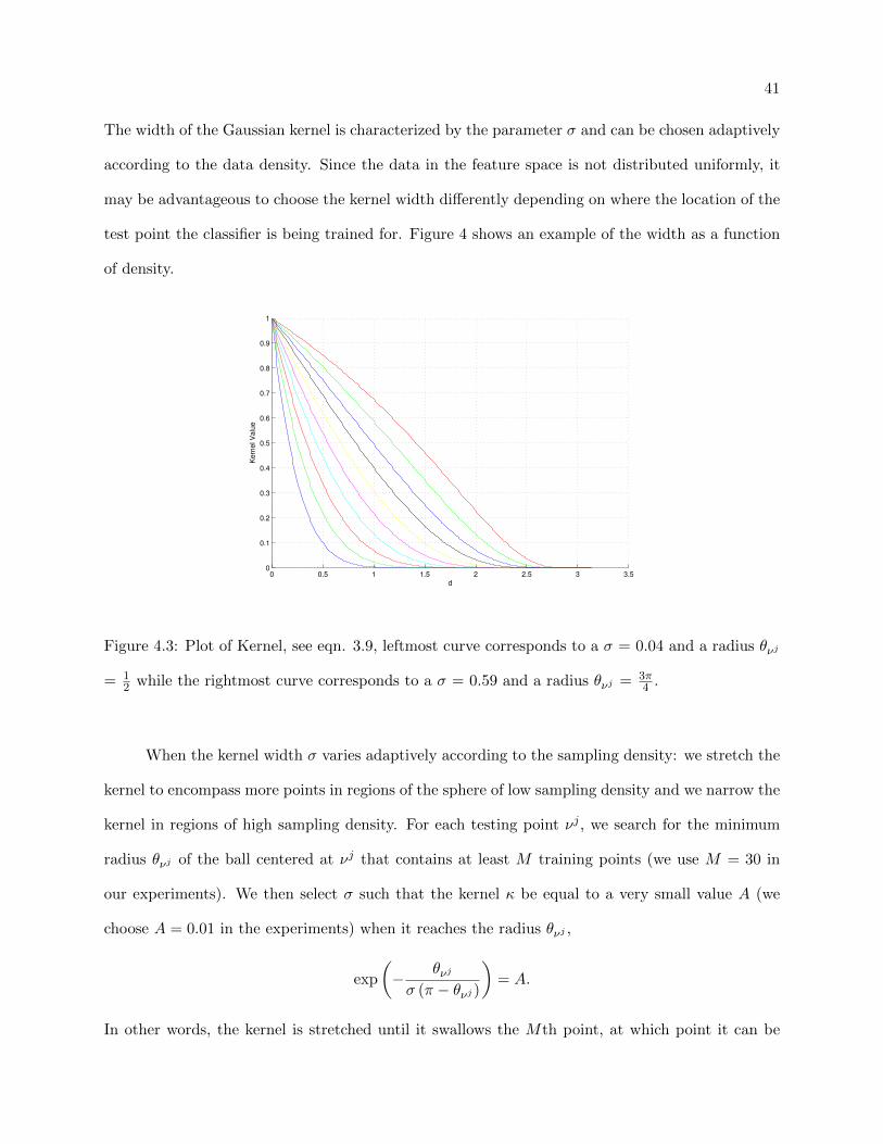
The width of the Gaussian kernel is characterized by the parameter σ and can be chosen adaptively

according to the data density. Since the data in the feature space is not distributed uniformly, it

may be advantageous to choose the kernel width differently depending on where the location of the

test point the classifier is being trained for. Figure 4 shows an example of the width as a function

of density.

0 0.5 1 1.5 2 2.5 3 3.50

0.1

0.2

0.3

0.4

0.5

0.6

0.7

0.8

0.9

1

d

Kern

el V

alu

e

Figure 4.3: Plot of Kernel, see eqn. 3.9, leftmost curve corresponds to a σ = 0.04 and a radius θνj

= 12 while the rightmost curve corresponds to a σ = 0.59 and a radius θνj = 3π

4 .

When the kernel width σ varies adaptively according to the sampling density: we stretch the

kernel to encompass more points in regions of the sphere of low sampling density and we narrow the

kernel in regions of high sampling density. For each testing point νj , we search for the minimum

radius θνj of the ball centered at νj that contains at least M training points (we use M = 30 in

our experiments). We then select σ such that the kernel κ be equal to a very small value A (we

choose A = 0.01 in the experiments) when it reaches the radius θνj ,

exp

(− θνj

σ (π − θνj )

)= A.

In other words, the kernel is stretched until it swallows the Mth point, at which point it can be

42

very small. This requirement leads to the following expression for σ,

σνj = − θνj

ln(A)(π − θνj ). (4.1)

Using this approach to account for the sampling density at each test point allows us to train

a classifier for each test point on each decomposition scale j. For each testing point, we search for

the appropriate value of σ and then train the respective classifier for that test point. An alternative

approach is to set the level of σ and apply the same kernel to each test point. We have implemented

each of these regimes for selecting the kernel width.

4.5 Classification Results

Our experiments consist of two binary classification scenarios: (1) Pn wave vs. Lg wave, and

(2) Pg wave vs. Lg wave. In each scenario, we classify two different types of seismic waves: primary

compressional (P) waves and surface (L) waves. The distinctions between a Pn and Pg wave are

related to the path along which the wave travels from the source to the observation point and the

type of reflections it experiences. For instance, a Pn wave travels along the boundary between the

crust and the mantle, while a Pg wave travels only through the crust. The Lg wave is a surface

wave that only travels through the crust.

We compared two different approaches for combining the classification results at all scales j:

entropy weighted and uniformly weighted. The general weighted model is given by

l∑j=1

wjfj(νj), (4.2)

where wj = (1 − hj(νj)) corresponds to the entropy weighted case and wj = 1 is the uniformly

weighted case. We report the classification accuracy for the three classification methods and several

choices of the wavelet filters. We also employ two strategies for selecting the kernel width parameter

(1) holding σ constant and (2) selecting σ adaptively according the sample density. Tables 4.1 - 4.4

show the classification results for both weightings and kernel width selection methods. Note that

the use of the kernel does not affect the k -NN method. However, equation 4.1 may be solved for

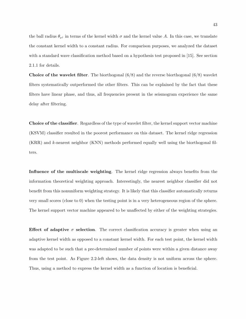
43

the ball radius θνj in terms of the kernel width σ and the kernel value A. In this case, we translate

the constant kernel width to a constant radius. For comparison purposes, we analyzed the dataset

with a standard wave classification method based on a hypothesis test proposed in [15]. See section

2.1.1 for details.

Choice of the wavelet filter. The biorthogonal (6/8) and the reverse biorthogonal (6/8) wavelet

filters systematically outperformed the other filters. This can be explained by the fact that these

filters have linear phase, and thus, all frequencies present in the seismogram experience the same

delay after filtering.

Choice of the classifier. Regardless of the type of wavelet filter, the kernel support vector machine

(KSVM) classifier resulted in the poorest performance on this dataset. The kernel ridge regression

(KRR) and k-nearest neighbor (KNN) methods performed equally well using the biorthogonal fil-

ters.

Influence of the multiscale weighting. The kernel ridge regression always benefits from the

information theoretical weighting approach. Interestingly, the nearest neighbor classifier did not

benefit from this nonuniform weighting strategy. It is likely that this classifier automatically returns

very small scores (close to 0) when the testing point is in a very heterogeneous region of the sphere.

The kernel support vector machine appeared to be unaffected by either of the weighting strategies.

Effect of adaptive σ selection. The correct classification accuracy is greater when using an

adaptive kernel width as opposed to a constant kernel width. For each test point, the kernel width

was adapted to be such that a pre-determined number of points were within a given distance away

from the test point. As Figure 2.2-left shows, the data density is not uniform across the sphere.

Thus, using a method to express the kernel width as a function of location is beneficial.

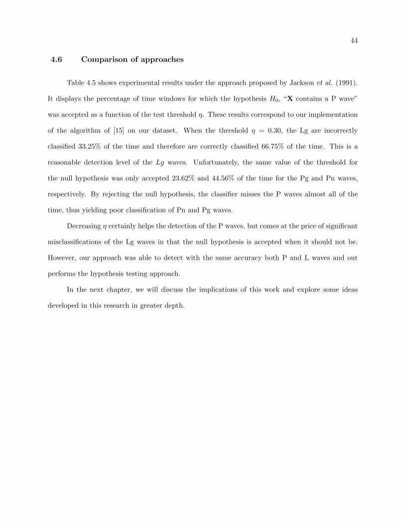
44

4.6 Comparison of approaches

Table 4.5 shows experimental results under the approach proposed by Jackson et al. (1991).

It displays the percentage of time windows for which the hypothesis H0, “X contains a P wave”

was accepted as a function of the test threshold η. These results correspond to our implementation

of the algorithm of [15] on our dataset. When the threshold η = 0.30, the Lg are incorrectly

classified 33.25% of the time and therefore are correctly classified 66.75% of the time. This is a

reasonable detection level of the Lg waves. Unfortunately, the same value of the threshold for

the null hypothesis was only accepted 23.62% and 44.56% of the time for the Pg and Pn waves,

respectively. By rejecting the null hypothesis, the classifier misses the P waves almost all of the

time, thus yielding poor classification of Pn and Pg waves.

Decreasing η certainly helps the detection of the P waves, but comes at the price of significant

misclassifications of the Lg waves in that the null hypothesis is accepted when it should not be.

However, our approach was able to detect with the same accuracy both P and L waves and out

performs the hypothesis testing approach.

In the next chapter, we will discuss the implications of this work and explore some ideas

developed in this research in greater depth.

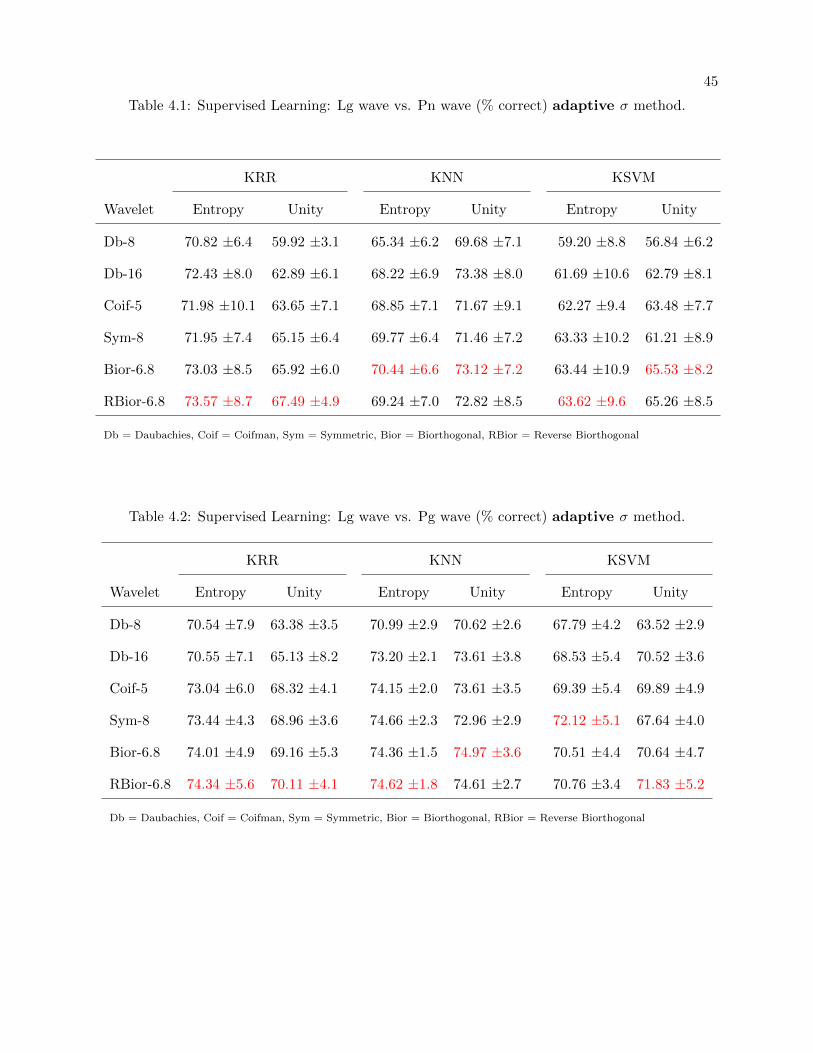
45

Table 4.1: Supervised Learning: Lg wave vs. Pn wave (% correct) adaptive σ method.

KRR KNN KSVM

Wavelet Entropy Unity Entropy Unity Entropy Unity

Db-8 70.82 ±6.4 59.92 ±3.1 65.34 ±6.2 69.68 ±7.1 59.20 ±8.8 56.84 ±6.2

Db-16 72.43 ±8.0 62.89 ±6.1 68.22 ±6.9 73.38 ±8.0 61.69 ±10.6 62.79 ±8.1

Coif-5 71.98 ±10.1 63.65 ±7.1 68.85 ±7.1 71.67 ±9.1 62.27 ±9.4 63.48 ±7.7

Sym-8 71.95 ±7.4 65.15 ±6.4 69.77 ±6.4 71.46 ±7.2 63.33 ±10.2 61.21 ±8.9

Bior-6.8 73.03 ±8.5 65.92 ±6.0 70.44 ±6.6 73.12 ±7.2 63.44 ±10.9 65.53 ±8.2

RBior-6.8 73.57 ±8.7 67.49 ±4.9 69.24 ±7.0 72.82 ±8.5 63.62 ±9.6 65.26 ±8.5

Db = Daubachies, Coif = Coifman, Sym = Symmetric, Bior = Biorthogonal, RBior = Reverse Biorthogonal

Table 4.2: Supervised Learning: Lg wave vs. Pg wave (% correct) adaptive σ method.

KRR KNN KSVM

Wavelet Entropy Unity Entropy Unity Entropy Unity

Db-8 70.54 ±7.9 63.38 ±3.5 70.99 ±2.9 70.62 ±2.6 67.79 ±4.2 63.52 ±2.9

Db-16 70.55 ±7.1 65.13 ±8.2 73.20 ±2.1 73.61 ±3.8 68.53 ±5.4 70.52 ±3.6

Coif-5 73.04 ±6.0 68.32 ±4.1 74.15 ±2.0 73.61 ±3.5 69.39 ±5.4 69.89 ±4.9

Sym-8 73.44 ±4.3 68.96 ±3.6 74.66 ±2.3 72.96 ±2.9 72.12 ±5.1 67.64 ±4.0

Bior-6.8 74.01 ±4.9 69.16 ±5.3 74.36 ±1.5 74.97 ±3.6 70.51 ±4.4 70.64 ±4.7

RBior-6.8 74.34 ±5.6 70.11 ±4.1 74.62 ±1.8 74.61 ±2.7 70.76 ±3.4 71.83 ±5.2

Db = Daubachies, Coif = Coifman, Sym = Symmetric, Bior = Biorthogonal, RBior = Reverse Biorthogonal

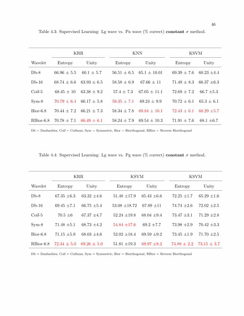
46

Table 4.3: Supervised Learning: Lg wave vs. Pn wave (% correct) constant σ method.

KRR KNN KSVM

Wavelet Entropy Unity Entropy Unity Entropy Unity

Db-8 66.96 ± 5.5 60.1 ± 5.7 56.51 ± 6.5 65.1 ± 10.01 69.39 ± 7.6 60.23 ±4.4

Db-16 68.74 ± 6.6 63.93 ± 6.5 58.58 ± 6.9 67.66 ± 11 71.49 ± 8.3 66.37 ±6.3

Coif-5 68.45 ± 10 63.38 ± 9.2 57.4 ± 7.3 67.05 ± 11.1 72.69 ± 7.2 66.7 ±5.3

Sym-8 70.79 ± 6.4 66.17 ± 5.8 59.35 ± 7.1 69.24 ± 9.9 70.72 ± 6.1 65.3 ± 6.1

Bior-6.8 70.44 ± 7.2 66.21 ± 7.3 58.34 ± 7.8 69.84 ± 10.1 72.43 ± 6.1 68.29 ±5.7

RBior-6.8 70.78 ± 7.1 66.49 ± 6.1 58.24 ± 7.9 69.54 ± 10.3 71.91 ± 7.6 68.1 ±6.7

Db = Daubachies, Coif = Coifman, Sym = Symmetric, Bior = Biorthogonal, RBior = Reverse Biorthogonal

Table 4.4: Supervised Learning: Lg wave vs. Pg wave (% correct) constant σ method.

KRR KSVM KSVM

Wavelet Entropy Unity Entropy Unity Entropy Unity

Db-8 67.35 ±6.3 63.32 ±4.6 51.48 ±17.9 65.43 ±6.6 72.25 ±1.7 65.29 ±1.6

Db-16 69.45 ±7.1 66.75 ±5.4 53.08 ±18.72 67.89 ±11 74.74 ±2.6 72.02 ±2.5

Coif-5 70.5 ±6 67.37 ±4.7 52.24 ±19.8 68.04 ±9.4 73.47 ±3.1 71.29 ±2.8

Sym-8 71.48 ±5.1 68.73 ±4.2 54.84 ±17.6 69.2 ±7.7 73.98 ±2.9 70.42 ±3.3

Bior-6.8 71.15 ±5.9 68.03 ±4.6 52.02 ±18.4 69.59 ±9.2 73.45 ±1.9 71.70 ±2.5

RBior-6.8 72.34 ± 5.0 69.26 ± 5.0 51.81 ±19.3 69.97 ±8.2 74.88 ± 2.2 73.15 ± 3.7

Db = Daubachies, Coif = Coifman, Sym = Symmetric, Bior = Biorthogonal, RBior = Reverse Biorthogonal

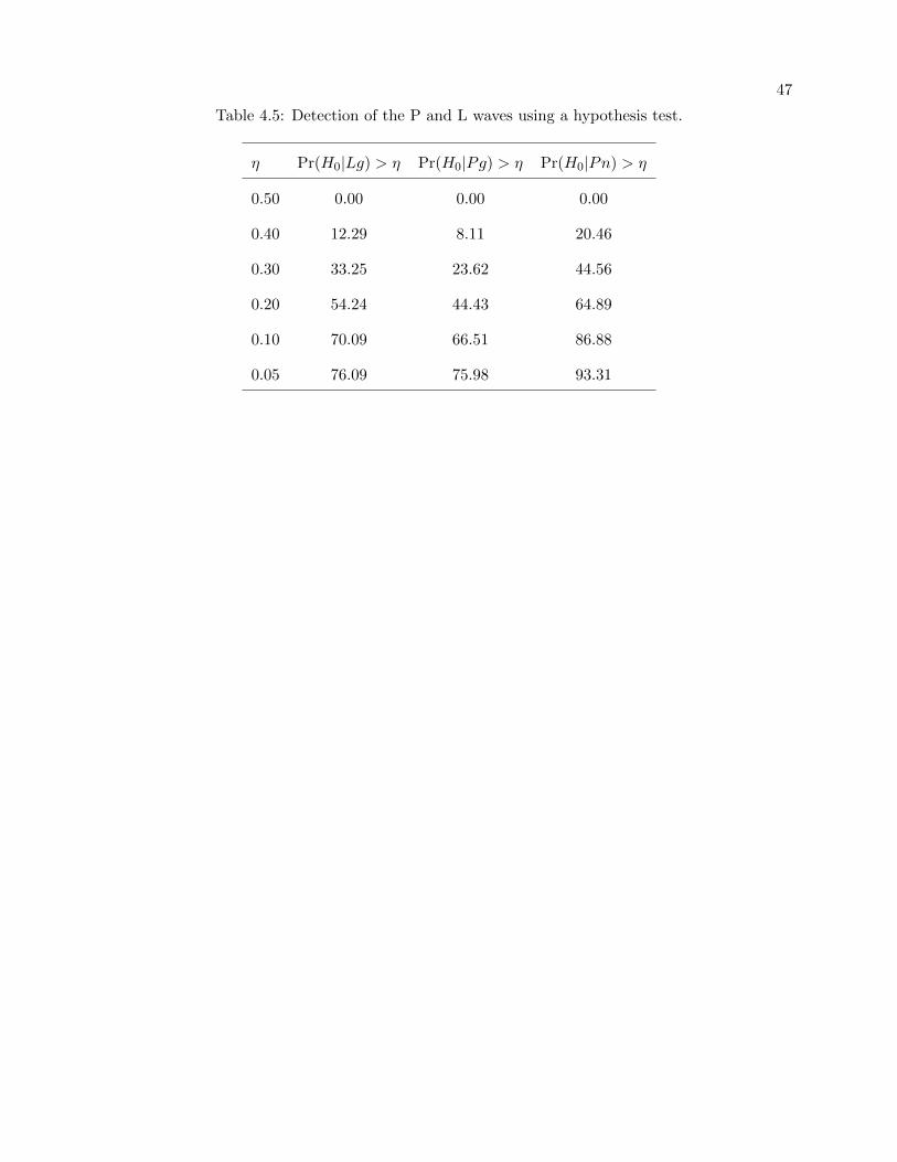
47

Table 4.5: Detection of the P and L waves using a hypothesis test.

η Pr(H0|Lg) > η Pr(H0|Pg) > η Pr(H0|Pn) > η

0.50 0.00 0.00 0.00

0.40 12.29 8.11 20.46

0.30 33.25 23.62 44.56

0.20 54.24 44.43 64.89

0.10 70.09 66.51 86.88

0.05 76.09 75.98 93.31

Chapter 5

Discussion and Conclusion

5.1 Discussion

Our approach to seismic phase classification consisted of two major parts: feature extraction

and supervised phase learning. In the first part, we are concerned with extracting the most con-

densed form phase describing features from the raw seismic signal. The second part focused is on

utilizing the structure in the feature space for phase classification.

The motivating factor for our approach is our initial hypothesis on seismic phases, which

states that in given segments of three-channel seismic signal where the waves in the windows are

of common phase, the waves in the window should share common features. The basis for this

hypothesis stems from the physics of seismic waves. Since natural seismic events occur from the

same underlying process, a slip at a fault in the Earth’s lithosphere, it is reasonable to infer

that phases share characterizing features. Phases represent motion in different directions. Our

experimental results suggest that we are on the right track since we see clustering among waves of

common phase in the feature space. Given the clustering in the multi-scale feature spaces (Figure

2.2-Left), we see that to some extent we are extracting a characterizing feature from the seismic

data. The polarization vector characterized the direction of dominant polarization. The remainder

of this chapter is dedicated to providing an understanding for the methods employed for phase

classification and ideas for extending this research.

The feature extraction stage can be thought of as a manifold learning step, where we seek a

low-dimensional parameterization of the data. In fact, our method achieves a dramatic reduction of

49

dimensionality. We map each 512×3 matrix of seismic data to a set of n+1 three-dimensional vectors

that captures different frequency content of the signal. These vectors each reside on a different

spherical manifold. This nonlinear transformation can be viewed as a non-linear dimensionality

reduction from the space of T × 3 matrices to multi-scale feature manifolds embedded in R3. As

seen in Figure 2.2-Left, the embedding seems to extracts a parameterization that describes the

phase of the seismic wave.

In the supervised phase learning stage, we have seen that despite the reduction in dimen-

sionality, enough physical information about each type of wave is preserved for the purpose of

classification. Since the manifold that is used to describe the data is a sphere, the real task was

to move classic supervised learning to this space. To accomplish this, we injected the geodesic

distance into the learning techniques where a distance measure was used. In our setting, we have a

closed form expression for this metric. In cases where the closed form is not accessible, the metric

would need to be exchanged with a procedure to estimate the geodesic distance. Extensions of

this work include the general problem of classifying points on a manifold. In general, one would

need to embed the manifold, using a bi-Lipschitz embedding, or estimate numerically the geodesic

distance.

Our experimental results show that even though we train our classifiers using seismic data

observed across a variety of regional recording stations, we are still able to distinguish between P

and L waves. These results suggest that the intrinsic physical differences that exist between the

P and L waves can be learned from a small set of regional recordings. Furthermore, the influence

of the local structure of the Earth surrounding the recording stations does not significantly reduce

our ability to learn the differences between P and L waves. Irrespective of the station from which

they were recorded, waves of the same type (P or L) form well-defined clusters in the feature space.

This is shown in Figure 2.2 and quantitatively verified by our experimental results.

The wavelet transform was the primary tool used for signal analysis. As the seismic signal is

of short duration, an accurate representation of this type of signal is achieved with a wavelet. The

motivating factor in using a wavelet transform is that it allows us to analyze a signal at multiple

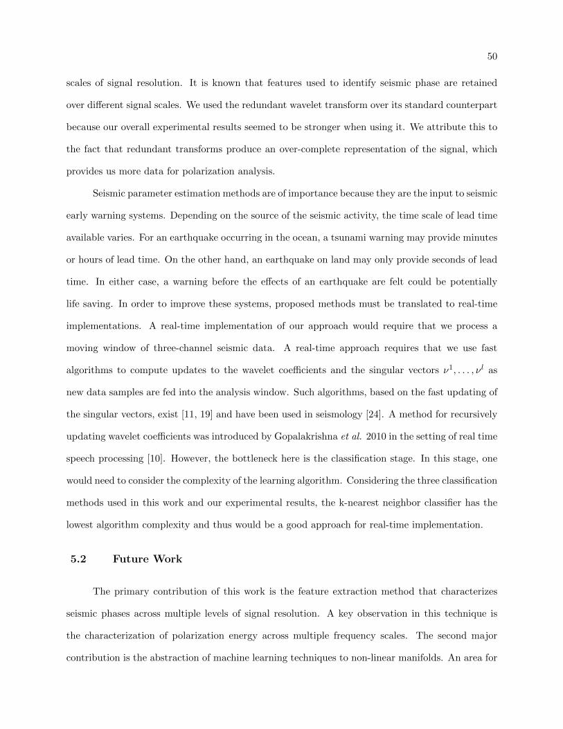
50

scales of signal resolution. It is known that features used to identify seismic phase are retained

over different signal scales. We used the redundant wavelet transform over its standard counterpart

because our overall experimental results seemed to be stronger when using it. We attribute this to

the fact that redundant transforms produce an over-complete representation of the signal, which

provides us more data for polarization analysis.

Seismic parameter estimation methods are of importance because they are the input to seismic

early warning systems. Depending on the source of the seismic activity, the time scale of lead time

available varies. For an earthquake occurring in the ocean, a tsunami warning may provide minutes

or hours of lead time. On the other hand, an earthquake on land may only provide seconds of lead

time. In either case, a warning before the effects of an earthquake are felt could be potentially

life saving. In order to improve these systems, proposed methods must be translated to real-time

implementations. A real-time implementation of our approach would require that we process a

moving window of three-channel seismic data. A real-time approach requires that we use fast

algorithms to compute updates to the wavelet coefficients and the singular vectors ν1, . . . , νl as

new data samples are fed into the analysis window. Such algorithms, based on the fast updating of

the singular vectors, exist [11, 19] and have been used in seismology [24]. A method for recursively

updating wavelet coefficients was introduced by Gopalakrishna et al. 2010 in the setting of real time

speech processing [10]. However, the bottleneck here is the classification stage. In this stage, one

would need to consider the complexity of the learning algorithm. Considering the three classification

methods used in this work and our experimental results, the k-nearest neighbor classifier has the

lowest algorithm complexity and thus would be a good approach for real-time implementation.

5.2 Future Work

The primary contribution of this work is the feature extraction method that characterizes

seismic phases across multiple levels of signal resolution. A key observation in this technique is

the characterization of polarization energy across multiple frequency scales. The second major

contribution is the abstraction of machine learning techniques to non-linear manifolds. An area for

51

further work is in the analysis of the distribution of data in the feature space.

The data exhibits structure in the locations of different classes over the sphere. An area of

extension may be to perform a statistical analysis in the areas of class density in the feature space.

This may provide a better understanding in the directions of maximum polarization characterized

during feature extraction.

In addition, we have demonstrated several supervised learning techniques over the feature

space. However, we did not perform an exhaustive survey of all the supervised learning techniques.

To extend this work, an analysis including stochastic learning methods, as well as alternate kernel

methods, could provide more examples to compare against our initial experimental results.

Overall, we set the groundwork for machine learning methods in the field of seismology. As

examples of the application areas become more apparent, the impact machine learning can have to

solve interesting problems will increase.

5.3 Conclusion

Our goal in this work was to explore the use of machine learning as it applies to seismology.

In particular, we discovered a transformation that takes windows of three-channel seismic data

and embeds them on the unit sphere across multiple frequency scales such that the location of

the embedding describes the seismic phase content in the wave. The utility of this transformation

is centered on the phase clustering in the feature space. Essentially, windows of seismic data

corresponding to the same seismic phase class tend to be physically located near each other in

the feature space. Having this type of structure over the feature space at different levels of signal

resolution provides a strong foundation for the application of supervised learning techniques for

phase classification. In addition, the simple geometric structure of the feature space allows for

supervised learning techniques to be translated directly to the feature space. In essence, we have

shown how to “lift” learning techniques to a non-linear manifold.

Bibliography

[1] R.V. Allen. Automatic phase pickers: Their present use and future prospects. Bull. Seism.Soc. Am., 68:1521–1532, 1982.

[2] E. Alpaydin. Introduction to machine learning. The MIT Press, 2004.

[3] K. S. Anant and F. U. Dowla. Wavelet Transform Methods for Phase Identification in Three-Component Seismograms. Bulletin of the Seismological Society of America, 87(6):1598–1612,1997.

[4] A. Bonfiglio. Wearable Monitoring Systems. Springer Verlag, 2010.

[5] K. Bullen and B. Bolt. An introduction to the theory of seismology. Cambridge UniversityPress, 1985.

[6] C. Burrus, R. Gopinath, and H. Guo. Introduction to Wavelets and Wavelet Transforms: APrimer. Prentice Hall, 1998.

[7] L. D’Auria, F. Giudicepietro, M. Martini, M. Orazi, R. Peluso, and G. Scarpato. Polarizationanalysis in the discrete wavelet domain: An application to volcano seismology. Bulletin of theSeismological Society of America, 100(2):670, 2010.

[8] R. Di Stefano, F. Aldersons, E. Kissling, P. Baccheschi, C. Chiarabba, and D. Giardini. Au-tomatic seismic phase picking and consistent observation error assessment: application to theItalian seismicity. Geophys. J. Intern., 165(1):121–134, 2006.

[9] P. Gendron, J. Ebel, and D. Manolakis. Rapid joint detection and classification with waveletbases via Bayes theorem. Bull. Seism. Soc. Am., 90(3):764, 2000.

[10] V. Gopalakrishna, N. Kehtarnavaz, and P.C. Loizou. A recursive wavelet-based strategy forreal-time cochlear implant speech processing on pda platforms. Biomedical Engineering, IEEETransactions on, 57(8):2053–2063, 2010.

[11] M. Gu and S.C. Eisenstat. A stable and fast algorithm for updating the singular value decom-position. New Haven: Yale University Department of Computer Science. RR-939, 1993.

[12] L. Hamber. Mr. lee geography and biology : http://mrleehamber.fusedfiber.com/unit%202.htm,April 2012.

[13] T. Hastie, R. Tibshirani, and J. Friedman. The Elements of Statistical Learning. SpringerVerlag, 2009.

53

[14] A.J. Izenman. Modern multivariate statistical techniques: regression, classification, andmanifold learning. Springer Verlag, 2008.

[15] G. M. Jackson, I. M. Mason, and S. A. Greenhalgh. Principle Component Transforms ofTriaxial Recordings by Singular Value Decomposition. Geophysics, 56(4):528–533, 1991.

[16] E. R. Kanasewich. Time Sequence Analysis In Geophysics. The University of Alberta Press,1985.

[17] P. Kumar and E. Foufoula-Georgiou. Wavelet Analysis for Geophysical Applications. Reviewsof Geophysics, 35(4):385–412, 1997.

[18] S. Mallat. A Wavelet Tour of Signal Processing. Academic Press, 1999.

[19] M. Moonen, P. Van Dooren, and J. Vandewalle. A singular value decomposition updatingalgorithm for subspace tracking. SIAM Journal on Matrix Analysis and Applications, 13:1015,1992.

[20] DTAM Project Team NASA. Seismicity:http://denali.gsfc.nasa.gov/dtam/seismic/.

[21] C. Panagiotakis, E. Kokinou, and F. Vallianatos. Automatic P -Phase Picking Based on Local-Maxima Distribution. IEEE Trans. Geosci. Remote Sens., 46(8):2280–2287, 2008.

[22] J. Park, F. L. Vernon III, and C. R. Lindburg. Frequency Dependent Polarization of High-Frequency Seismograms. Journal of Geophysical Research, 92(B12):12,664–12,674, 1987.

[23] J. Ramirez Jr and F.G. Meyer. Machine learning for seismic signal processing: Phase classifica-tion on a manifold. In Proceedings of the 10th International Conference on Machine Learningand Applications, pages 382–388. IEEE, 2011.

[24] A. Rosenburg. Real-Time Ground-Motion Analysis: Distinguishing P and S Arrivals in a NoisyEnvironment. Bulletin of the Seismological Society of America, 100(3):1252–1262, 2010.

[25] C.D. Saragiotis, L.J. Hadjileontiadis, and S.M. Panas. A higher-order statistics-based phaseidentification of three-component seismograms in a redundant wavelet transform domain. InHigher-Order Statistics, 1999. Proceedings of the IEEE Signal Processing Workshop on, pages396–399. IEEE, 1999.

[26] P. Shearer. Introduction to Seismology. Cambridge University Press, 2006.

[27] M.J. Shensa. The discrete wavelet transform: Wedding the a trous and Mallat algorithms.IEEE Trans. on Signal Processing, 40(10):2464–2482, 1992.

[28] S. Sommer, F. Lauze, S. Hauberg, and M. Nielsen. Manifold valued statistics, exact principalgeodesic analysis and the effect of linear approximations. Computer Vision–ECCV 2010, pages43–56, 2010.

[29] S. Stein and M. Wysession. An Introduction to Seismology Earthquakes and Earth Structure.Blackwell Publishing, 2003.

[30] United States Geographical Survey. Tectonic plates:http://pubs.usgs.gov/publications/text/slabs.htm, February 1996.

54

[31] United States Geographical Survey. Inside the earth:http://pubs.usgs.gov/gip/dynamic/inside.html, May 1999.

[32] United States Geographical Survey. Earthquake hazards program:http://earthquake.usgs.gov/earthquakes/eqarchives/year/eqstats.php, April 2012.

[33] K. M. Taylor, M. J. Procopio, C. J. Young, and F. G. Meyer. Estimation of arrival times fromseismic waves: a manifold based approach. Geophysical Journal International, 185:435–452,2011.

[34] I. M. Tibuleac, E. T. Herrin, J. M. Britton, R. Shumway, and A. C. Rosca. Automatic Sec-ondary Seismic Phase Picking Using the Wavelet Transform. Seismological Research Letters,74(6):884–892, 2003.

[35] P. Turaga, A. Veeraraghavan, and R. Chellappa. Statistical analysis on stiefel and grassmannmanifolds with applications in computer vision. In Computer Vision and Pattern Recognition,2008. CVPR 2008. IEEE Conference on, pages 1–8. IEEE, 2008.

[36] K. Walker. Science and technology review, sleuthing seismic signals. Technical report,Lawrence Livermore National Lab., CA (US), 2009.

[37] Wikipedia. Learning: http://en.wikipedia.org/wiki/learning, April 2012.

[38] M. Withers, R. Aster, C. Young, J. Beiriger, M. Harris, S. Moore, and J. Trujillo. A comparisonof select trigger algorithms for automated global seismic phase and event detection. Bull. seism.Soc. Am., 88(1):95–106, Feb. 1998.

[39] H. Zhang, C. Thurber, and C. Rowe. Automatic P-wave arrival detection and picking withmultiscale wavelet analysis for single-component recordings. Bull. Seism. Soc. Am., 93(5):1904,2003.

[40] M. N. Zhizhin, D. Rouland, J. Bonnin, A. D. Gvishiani, and A. Burtsev. Rapid Estimation ofEarthquake Source Parameters from Patter Analysis of Waveforms Recorded at a Single Three-Component Broadband Station. Bulletin of the Seismological Society of America, 96(6):2329–2347, 2006.