Josué Diwambuena, Francesco Ravazzolo

BEMPS –Bozen Economics & ManagementPaper Series

NO 86/ 2021

Identification of Labour Market Shocks

Josué Diwambuena, Francesco Ravazzolo

Identification of Labour Market Shocks*

Josué Diwambuena † Francesco Ravazzolo ‡

June 15, 2021

Abstract

We propose a structural VAR model using sign restriction identification to disentangle sup-

ply, demand, and shocks originating from the labour market, and to quantify their relevance

for economic fluctuations. We estimate our model on Italy’s data from 2000Q1 to 2018Q4

using Bayesian techniques. Our results are as follows. First, wage bargaining and labour sup-

ply shocks are among the largest drivers of output and labour market fluctuations both at short

and long horizons. Second, matching efficiency and automation shocks are critical drivers

of labour market fluctuations but they have limited relevance for business cycle fluctuations.

Our results are robust across many alternative specifications including a large SVAR model

using a factor-based sign restriction identification estimated with a computationally efficient

algorithm recently proposed by Korobilis (2020). Given the burgeoning significance of labour

market shocks, we suggest that policies aimed at improving the flexibility of Italy’s labour

market should be strengthened.

JEL Codes: C11, C32, E32.

Keywords: Labour market shocks, SVAR, Sign restriction.

*We are grateful to Massimiliano Pisani for his detailed comments on the preliminary version of this paper duringhis discussion at the 8th SIdE-IEA Workshop for PhD Students in Econometrics and Empirical Economics. We havebenefited from discussions with Francesco Furlanetto, Luca Gambetti, Emanuele Bacchiocchi and Marco Lombardi.Finally, we would like to thank participants at the 9th Italian Congress of Econometrics and Empirical Economics;the 8th SIdE Workshop for PhD students in Econometrics and Empirical Economics; and various conferences andresearch seminars for their useful comments.

†Corresponding author. Address: Free University of Bozen-Bolzano. Building E-511. Piazza Università 1,Bolzano, Italy. E-mail: [email protected]

‡Free University of Bozen-Bolzano, CAMP, BI Norwegian Business School, RCEA. Building E-207. PiazzaUniversità 1, Bolzano, Italy. E-mail: [email protected]

1

[email protected]

[email protected]

1 Introduction

In this paper, we propose a structural vector autoregressive (SVAR) model using sign restriction identifi-

cation to disentangle supply, demand, and shocks originating from the labour market and to measure their

significance for economic fluctuations. Previous studies in the literature mainly identify productivity shocks

within the context of dynamic stochastic general equilibrium (DSGE) and or SVAR models relying on re-

cursive identification methods.

Seminal papers by Gali (1999), Christiano, Eichenbaum & Vigfusson (2004); Francis & Ramey (2005)

construct small SVAR models and rely on long-run identification as in Blanchard & Quah (1989) to examine

the response of hours to productivity shocks in the US. Fisher (2006) studies the behaviour of hours to neutral

and investment-specific productivity shocks in the US using the same identification method. Recently,

Galí & Gambetti (2009) and Cantore, Ferroni & Leon-Ledesma (2017) document time-varying patterns in

hours in the US post-war era and setup a Time-Varying parameter VAR model (TVP-VAR) using the same

identification strategy to assess the response of hours to productivity shocks.

In the last two decades, empirical studies have greatly relied on sign restriction identification strategy to

identify many shocks. For example, Faust (1998) and Uhlig (2005) identify monetary policy shocks. Gam-

betti (2006) and Peersman & Straub (2009) disentangle the impact of productivity shocks. Mountford &

Uhlig (2009) and Pappa (2009) study the effects of government spending shocks. Fujita (2011) and Foroni,

Furlanetto & Lepetit (2018) mainly examine the relevance of labour market shocks for economic fluctua-

tions. Furlanetto & Robstad (2019) scrutinize the contribution of immigration shocks for economic volatility

in Norway. Baumeister & Peersman (2013) and Kilian & Murphy (2012) assess how oil price shocks influ-

ence output fluctuations. Gambetti & Musso (2017) and Furlanetto, Ravazzolo & Sarferaz (2019) evaluate

the role of financial shocks for economic variability. Benati & Lubik (2014) develop a TVP-VAR models

with stochastic volatility to investigate the interaction between Beveridge curve dynamics and the macroe-

conomy in the US.

For Italy, we find very few studies that document the macroeconomic effects of shocks on labour market

dynamics using SVAR models.1 Previous studies that quantify the primacy of labour market shocks for eco-

nomic fluctuations within the context of SVAR models using sign restriction identification are rather small

or medium-scaled models and identify too few shocks (i.e. at most four shocks). In the recent literature,

we find very few many papers that identify several shocks (i.e. at least five shocks) using sign restriction

identification.2 Furlanetto, Ravazzolo & Sarferaz (2019) and Foroni, Furlanetto & Lepetit (2018) are the

most relevant studies for this paper.

The contribution of this paper is as follows. First, we offer a methodological contribution to the busi-

ness cycle literature that evaluates the effects of shocks on labour market dynamics within the context of

1Gambetti & Pistoresi (2004) and Di Giorgio & Giannini (2012) are the rare exception in the literature and mainlyrely on recursive identification methods. Gambetti & Pistoresi (2004) estimate a small SVAR model to identify theeffects of productivity, demand and markup shocks in Italy. Di Giorgio & Giannini (2012) apply a Vector ErrorCorrection (VECM) model to examine Beveridge curve dynamics between the US and Italy.

2Furlanetto, Ravazzolo & Sarferaz (2019) and Foroni, Furlanetto & Lepetit (2018) are exceptions in the literature.

2

SVAR models using sign restriction identification scheme as in Furlanetto, Ravazzolo & Sarferaz (2019) and

Foroni, Furlanetto & Lepetit (2018). In this regard, we use many alternative SVAR specifications to gauge

the importance of shocks for economic fluctuations and to check the robustness of our results. Second, we

disentangle the macroeconomic effects of supply, demand and labour market shocks and we quantify their

contributions for economic fluctuations. Our identification strategy assumes no a priori strong contribution

of productivity shocks as in Gali (1999). Third, we estimate our model on Italy’s data using Bayesian tech-

niques and we derive our robust sign restrictions from the DSGE literature3 and numerous SVAR studies4

that examine the interaction between labour market dynamics and the business cycle. Fourth, given recent

promising labour market trends on the Italian labour force participation (cf. De Philippis 2017) and job

matching efficiency (see Pinelli et al. 2017), we identify shocks that mimic these changes and we study their

macroeconomic effects on labour market dynamics as in Foroni, Furlanetto & Lepetit (2018).

Our results are as follows. First, we confirm that wage bargaining and labour supply shocks are among the

greatest drivers of output and labour market fluctuations both at short and long horizons. Second, matching

efficiency and automation shocks are significant contributors to labour market fluctuations but they have

limited relevance for output fluctuations. Third, although we stress the relevance of labour market shocks, we

also discover that productivity, demand and investment shocks are also key drivers of economic fluctuations

across horizons. Our results are robust across several alternative SVAR specifications including a large

SVAR model using a factor-based sign restriction identification estimated with a computationally efficient

algorithm recently proposed by Korobilis (2020).

The remainder of this paper is structured as follows. Section 2 reviews the stylized facts of the Italian

labour market. Section 3 explains the structural VAR model and the sign restriction identification strategy.

Section 4 presents the results of the baseline model and those of the robustness check. Section 5 analyzes

the response of Italy’s labour force participation to shocks. Section 6 uses data on vacancies to identify

a matching efficiency shock. In section 7, we disentangle an automation shock from other labour market

shocks. Section 8 estimates a large SVAR using a factor-based sign restriction identification. Section 9

provides concluding remarks and formulates some policy suggestions.

2 Stylized facts of the Italian Labour Market

Italy has experienced several episodes of slowdown in labour productivity growth during the last two decades

(Daveri et al. 2005; Hall et al. 2009). Figure 1 plots the evolution of labour productivity per hours worked

(labour productivity) indices in Italy and the US from 2000Q1 to 2018Q4. These series are taken from

Eurostat and FRED and are defined as the ratio of real output per total number of hours worked. The grey

shaded area denotes the 2008-2009 recession period in the US. This figure shows that labour productivity in

3Furlanetto, Ravazzolo & Sarferaz (2019); Furlanetto & Groshenny (2016), Zhang (2017), Galí, Smets & Wouters(2012), Justiniano, Primiceri & Tambalotti (2013).

4Diamond & Blanchard (1989), Chang & Schorfheide (2003), Peersman & Straub (2009), Canova & Paustian(2011), Benati & Lubik (2014), Foroni, Furlanetto & Lepetit (2018), Furlanetto, Ravazzolo & Sarferaz (2019), Furlan-etto & Robstad (2019).

3

Italy has been higher than in the US in the pre-Great Recession (GR) era (2000-2006). In the post-GR era,

labour productivity in Italy remains slightly below the US level but converges. We observe a peculiar trend

during the GR era. In fact, during this period, labour productivity in Italy has significantly declined below

the US level. A number of studies in the literature try to explain this drop in labour productivity growth

using a microeconometric approach (e.g. Daveri et al. 2005; Pianta & Vaona 2007; Brandolini et al. 2007;

European Commission 2006).

Daveri et al. (2005) attribute the plunge in labour productivity growth to the decline in total factor pro-

ductivity (TFP). Pianta & Vaona (2007) think that the exhaustion of capital deepening is responsible for

this slowdown. For Brandolini et al. (2007), this deceleration is triggered by resource reallocation arising

from labour market reforms which have changed the relative price of labour with respect to capital. The

European Commission (2006) identifies insufficient research and development (R&D) investment by Italian

firms as a potential source of this plummet. The Italian labour market is mostly known for its dualistic

nature. Italy’s labour market is characterized by a low level of employment for women and the youth; great

disparity between the Northern and the Southern regions; high skill mismatch and a highly centralized rigid

wage collective bargaining mechanism (Ciccarone et al. 2016; Adda et al. 2017; Schrader & Ulivelli 2017).

To mitigate these shortcomings and create conditions that are conducive to high labour productivity, Italy

undertook several reforms (Schrader & Ulivelli 2017; Pinelli et al. 2017).5

The Job Act, which builds from the Fornero reform, is the most recent reform executed in 2015 and was

aimed at improving job matching efficiency (Pinelli et al. 2017). Pinelli et al. (2017) support that after the

enactment of the Job Act, the number of permanent jobs positions rose substantially in 2015, labour market

duality was reduced and job matching efficiency was significantly enhanced.

Despite these promising labour market trends, the slowdown in labour productivity growth remains a great

concern for policymakers. While microeconomic evidence offers insightful explanations on this puzzle, we

think that a macroeconometric approach is needed in order to evaluate the response of labour productivity to

shocks, to quantify their relevance for economic fluctuations and eventually to derive possible implications

for macroeconomic policies. In the business cycle literature for Italy, previous studies analyze the effects of

shocks on labour productivity and quantify their significance by applying recursive identification strategies

(e.g. Gavosto & Pellegrini 1999; Gambetti & Pistoresi 2004; Di Giorgio & Giannini 2012). As an example,

Gambetti & Pistoresi (2004) identify productivity, demand and markup shocks and show that demand and

markup shocks are the most significant drivers of output fluctuations. They find out that the productivity

shock only accounts for a marginal share of output fluctuations. Di Giorgio & Giannini (2012) evaluate

Beveridge curve dynamics in the US and Italy through a cointegrated VAR model. They discover that the

labour supply shock is the major driver of unemployment fluctuations in the US in the long-run whereas this

role is played by reallocation shocks in Italy. They also find the productivity shock to be an important driver

of unemployment variability in both countries.

5Labour market reforms include among others the collective bargaining framework and wage indexation; the TreuPackage (1997); the 2003 Biagi Law; the Fornero reform and lately the Job Act.

4

2000 2002 2004 2006 2008 2010 2012 2014 2016 2018

Year

95

96

97

98

99

100

101

Lab

or

Pro

du

ctiv

ity

Ind

ex

70

75

80

85

90

95

100

105

110

ItalyUS

Figure 1 – Labour Productivity in Italy and US (2000Q1-2018Q4).

3 The VAR Model and the Identification Strategy

We consider the following reduced-form VAR representation:

Yt =CA +P

∑i=1

AiYt−i + εt (1)

where Yt is a (N× 1) vector containing all N endogenous variables, CA is a (N× 1) vector of constants,

Ai for i = 1, ...,P are (N×N) matrices of parameters. P denotes the optimal number of lags and εt is a

(N × 1) vector of reduced form residuals with εt ∼ N (0,Σ) where Σ is a (N ×N) variance-covariance

matrix. Given large parameter uncertainty, we estimate our model parameters with Bayesian techniques.

Our model is specified and estimated in level since Bayesian methods can be applied regardless of the

presence of non-stationarity in data (Sims et al. 1990). We specify diffuse priors so that the information

in the likelihood function becomes dominant. Our priors lead a Normal-Inverse Wishart posterior with the

mean and variance parameters corresponding to OLS estimates. To recover the effects of structural shocks,

we map our reduced-form innovations εt to be written as a linear combination of structural disturbances ηt

such that:

εt = Sηt (2)

5

where ηt denotes a (N × 1) vector of structural-form disturbances with ηt ∼ N (0,Ω) and Ω = I. The

variance-covariance matrix in (2) admits the following structure Σ = SS′. Applying a Cholesky decompo-

sition restricts S to be lower triangular, thereby implying a recursive identification procedure. Recently, the

sign-restriction identification has gained popularity in identifying structural shocks (Faust 1998, Canova &

De Nicolo 2002, Peersman 2005, Uhlig 2005, Fry & Pagan 2011). To identify our structural shocks using

the sign restriction identification strategy, we use the algorithm proposed by Rubio-Ramirez, Waggoner &

Zha (2010). Further details regarding the Bayesian estimation and the sign restriction identification can be

found in the appendix A.1. We impose restrictions on impact only since these are sufficient to separately

identify many shocks (Canova & De Nicolo 2002).

Table 1 summarizes the restrictions imposed in our baseline model. In this specification, we disentangle

supply and demand shocks from labour market shocks. We identify one supply shock (productivity shock),

two demand shocks6 and two labour market shocks. Our baseline model includes six endogenous variables

and five identified shocks. Our identifying restrictions are taken from the literature that evaluates the in-

teraction between labour market dynamics and the business cycle (Canova & Paustian 2011; Furlanetto &

Robstad 2019; Foroni, Furlanetto & Lepetit 2018; Furlanetto, Ravazzolo & Sarferaz 2019).

Table 1 – Sign restrictions

Supply Demand Wage Barg. Labour Supply InvestmentGDP + + + + +Labour Productivity NA NA NA NA NAPrices - + - - +Real Wages + NA - - NAUnemployment NA - - + -Investment/GDP NA - + NA +

Table describes the restrictions used for each variable (in rows) to identified shocks (in columns) in our VAR. + and - denote positive and negative restriction respectively. NA denotesunrestricted.

We normalize the response of output to all shocks to be positive across horizons. We impose that a positive

productivity shock has a positive effect on real wages and generates countercylical co-movement of output

and prices. We leave unrestricted the responses of unemployment and investment to productivity shocks

since their effects are not clear in the literature. A positive demand shock is a disturbance that pushes up

output and prices but diminishes unemployment and investment. Demand and investment shocks are sepa-

rately identified by imposing opposite signs on the response of investment. We assume that our investment

shock is the only demand disturbance that drives up investment. All other restrictions for our demand shock

remain applicable for an investment shock. We leave unrestricted the response of real wages to demand and

investment shocks as their effects are not clear in the literature. The response of labour productivity to a pro-

ductivity shock depends on how hours are specified in the VAR model (Gali 1999; Christiano, Eichenbaum

& Vigfusson 2004).7 Due to this ambiguity, we leave its response unrestricted to all shocks.

6Our demand shock triggers an increase in any component of aggregate demand except investment. Furlanetto,Ravazzolo & Sarferaz (2019) interpret this as a fiscal shock, a shock to consumption or a foreign shock.

7Gali (1999) specifies growth hours and finds that labour productivity increases after a positive productivity shock.

6

Our expansionary wage bargaining shock is a disturbance that reduces worker’s bargaining power in the

Nash-bargaining wage negotiation and as a result, it shrinks real wages. This reduction is expected to

bring down prices as marginal costs are cut. We restrict unemployment to go down as we expect firms

to post more unfilled vacancies which enhances the job finding rate. In addition, we expect investment to

rise up as firms use the employment surplus to purchase physical capital, thereby expanding productivity

capacities. We disentangle a labour supply shock from a wage bargaining shock by using different sign

on the response of unemployment (Foroni, Furlanetto & Lepetit 2018). We impose that our labour supply

shock raises the number of unemployed people searching for jobs in the labour market, hence augmenting

labour force participation rate. A large share of job seekers make it hard to hire all unemployed people and

so unemployment hikes (Diamond & Blanchard 1989). The rise in the number of unemployed people allows

firms to cut marginal costs and to boost production since they fill up vacancies at much cheaper hiring costs.

We remain agnostic about the response of investment to the labour supply shock. To have a fully identified

model, we add a residual shock which is left unrestricted.

4 Empirical Results

In this section, we present the results obtained from the estimation of our baseline model. Our model

is estimated in level using Bayesian estimation techniques on Italy’s data from 2000Q1 to 2018Q4. Our

baseline model is estimated using five lags and six variables, i.e. real GDP, labour productivity, GDP deflator

as a measure of prices, unemployment rate, real wages and investment. All variables are expressed in natural

logs except unemployment rate. Data sources are described in Appendix A.3.

4.1 Baseline Model

Table 2, we show the forecast error variance decomposition of five identified shocks at three different hori-

zons. The forecast error variance decompositions are computed at each horizon on the median draw that

satisfies our sign restrictions.8

Our findings are as follows. Our identified labour market shocks explain a great share of economic fluctu-

ations across horizons. They account for more than 50 percent of output fluctuations at short and medium

horizons and 40 percent at long horizons. They represent more than 20 percent of labour productivity

variability at medium and long horizons. The investment shock is a major driver of labour productivity

Christiano et al. (2004) show that hours increase when specified in level while they decrease when they enter as growth.In the DSGE literature, a permanent productivity shock may exert either a positive or a negative effect on hours (Gali1999, Gambetti 2006, Cantore, Ferroni & Leon-Ledesma 2017). The RBC view supports that a positive productivityshock induces people to work more and consequently firms respond by raising hours. In contrast, the NK-DSGEview suggests that in the short-run, because output is demand constrained due to price and wage rigidities, the shockgenerates a fall in hours as firms lay off some workers.

8As highlighted by Fry & Pagan (2011), variance decompositions based on the median of impulse responsescombines the information coming from different models and does not necessarily sum to one across all shocks. As inFurlanetto, Ravazzolo & Sarferaz (2019), our variance decompositions are re-scaled so that the variance accounts forall shocks.

7

fluctuations. Labour market shocks are among the largest drivers of real wages and unemployment. They

explain at least 60 percent of volatility in unemployment at short horizons and 10 percent at long horizons.

Their contribution represent 50 percent of real wages volatility at short horizons and 40 percent at long

horizons. At least 30 percent of investment and prices volatility are driven by these shocks. The produc-

tivity shock explains only 20 percent of business cycle volatility at short horizons and around 30 percent at

medium and long horizons. It accounts for 20 percent of variability in labour productivity and 40 percent

of unemployment fluctuations at short horizons. The demand shock has a significant role on labour market

dynamics. It describes around 30 percent of labour productivity and real wages volatility at short horizons.

Table 2 – Median Forecast Error Variance Decomposition for the Baseline Model

Horizon Supply Demand Wage Barg Lab Supply Investment

GDP 1 0.17 0.10 0.26 0.28 0.195 0.32 0.05 0.14 0.34 0.1520 0.29 0.12 0.16 0.21 0.22

Labour Productivity 1 0.05 0.27 0.01 0.00 0.675 0.07 0.14 0.11 0.11 0.1520 0.17 0.10 0.11 0.15 0.46

Prices 1 0.29 0.13 0.32 0.12 0.145 0.23 0.20 0.22 0.11 0.2420 0.21 0.18 0.25 0.12 0.24

Wages 1 0.28 0.24 0.20 0.29 0.005 0.30 0.06 0.11 0.54 0.0020 0.15 0.17 0.18 0.24 0.26

Unemployment 1 0.08 0.12 0.33 0.34 0.125 0.45 0.05 0.16 0.09 0.2420 0.30 0.06 0.07 0.05 0.53

Investment 1 0.18 0.05 0.29 0.05 0.415 0.41 0.04 0.16 0.14 0.2620 0.29 0.06 0.09 0.09 0.47

Figures 2-3 present the impulse responses for these two labour market shocks. The labour supply shock

has a positive and significant effect on output. The rise in output is hump-shaped and temporary. This

shock triggers a permanent decline in labour productivity and real wages and a temporary fall in prices. The

decrease in real wages is statistically significant. The shock generates a temporary increase in unemployment

and in investment. Unemployment turns negative at long horizons. An expansionary labour supply shock

triggers procyclical co-movement of output and unemployment. It also generates a positive co-movement

of real wages and labour productivity. Our findings are consistent with previous evidence by Galí, Smets &

Wouters (2012) and Justiniano, Primiceri & Tambalotti (2013).9 The wage bargaining shock has a positive

and persistent effect on output. It generates a negative and persistent reduction in labour productivity, real

wages and unemployment for many quarters but leads to a temporary fall in prices.

9Galí et al. (2012) and Justiniano et al. (2013) argue that any shock that generates macroeconomic dynamics similarto a wage markup shock is a major driver of economic fluctuations across horizons.

8

1 5 10 15 20 25 30 35-5

0

5

10-3 GDP

1 5 10 15 20 25 30 35-0.01

0

0.01 Labor Productivity

1 5 10 15 20 25 30 35-2

0

210-3 Prices

1 5 10 15 20 25 30 35

-2

0

2

10-3 Wage

1 5 10 15 20 25 30 35

-0.2

0

0.2

Unemployment

1 5 10 15 20 25 30 35-0.02

0

0.02 Investment

Figure 2 – Impulse responses to a labour supply shock in the baseline model. The blue line represents the posterior median at each horizon and theshaded area indicates the 16th and 84th percentiles of the impulse responses.

The decline in unemployment is statistically significant before turning positive shortly at medium horizons

and then negative at long horizons. The collapse in real wages is also statistically significant before turning

positive at medium horizons. Our expansionary wage bargaining shock leads to a temporary and statistically

significant increase in investment.

Similar to the labour supply shock, our wage bargaining shock drives real wages and labour productivity in

the same direction. The fact that labour market shocks exert prolonged effects on labour productivity is at

odds with the idea that productivity shocks are the only source of long-run fluctuations in labour productivity

as stressed in Gali (1999).

9

1 5 10 15 20 25 30 35-5

0

510-3 GDP

1 5 10 15 20 25 30 35-0.01

0

0.01 Labor Productivity

1 5 10 15 20 25 30 35

-2

0

210-3 Prices

1 5 10 15 20 25 30 35

-2

0

2

10-3 Wage

1 5 10 15 20 25 30 35

-0.2

0

0.2 Unemployment

1 5 10 15 20 25 30 35-0.02

0

0.02 Investment

Figure 3 – Impulse responses to the wage bargaining shock in the baseline model. The blue line represents the posterior median at each horizon andthe shaded area indicates the 16th and 84th percentiles of the impulse responses.

Figure 4 plots the historical decomposition of labour productivity in which we exhibit the contribution of

each structural shock to the total forecast error variance at each point in time. Labour market shocks are

among the drivers that contribute to the increase in labour productivity over the entire sample period. The

role of the productivity shock in improving labour productivity is more pronounced in the pre-GR period.

During the GR period, labour markets shocks explain the large decline in labour productivity. In the post-GR

era, labour market shocks contribute to enhance labour productivity.

10

2002 2004 2006 2008 2010 2012 2014 2016-0.025

-0.02

-0.015

-0.01

-0.005

0

0.005

0.01

0.015

0.02

SupplyResidualDemandWage BargainingLabor SupplyInvestmentLabor Productivity Growth (w/o Baseline)

Figure 4 – Historical decomposition for the baseline model. The blue line denotes the deviation in productivity Growth from its Baseline Forecastfor the Period 2000–2018.

4.2 Baseline-Robustness Checks

In this sub-section, we check the robustness of our baseline results to a battery of sensitivity analysis. We

check the robustness of our results by (i) replacing labour productivity with hours, (ii) replacing aggregate

unemployment with unemployment by education levels and gender (iii) estimating our baseline model with

a different lag specification, (iv) using a large sample, and finally (v) using an alternative measure of central

tendency (i.e. the modal model suggested by Inoue & Kilian 2013). All our identifying restrictions imposed

on the baseline model remain unchanged. For the sake of exposition, we only present the results emerging

from the forecast error variance decompositions of all these specifications in Tables 11-22.

We replace labour productivity with hours to analyze the response of the latter to shocks. Since there is

no consensus in the literature on the macroeconomic effects of productivity shocks on hours, we choose to

leave its response unrestricted to all shocks. Table 11, we show the forecast error variance decomposition

of shocks in the baseline model including hours. We confirm that our labour market shocks are among the

greatest drivers of output and labour market dynamics across horizons. They account for more than half of

11

output volatility at short and long horizons. They explain at least 20 percent of fluctuations in hours at short

horizons and more than 30 percent at long horizons. Our baseline model is previously estimated with data

on aggregate unemployment. We now replace the latter with more disaggregate measures of unemployment.

Adda et al. (2017) document great disparities in unemployment rates in Italy between men and women and

for high-skilled, middle-skilled and low-skilled individuals. They show that on average that unemployment

is higher for women than men and that less educated individuals are prone to high unemployment level

compared to the other groups. Hence, we study the responses of unemployment for three educational levels:

(a) less than primary, primary and lower secondary education, (b) upper secondary and post-secondary non-

tertiary education and (c) tertiary education. We proxy these groups as low-skill, middle-skill and high-skill

respectively. Then, we examine the responses of unemployment by gender (men and women). We check the

robustness of our baseline results by introducing disaggregate measures of unemployment one after another.

Tables 12-14 summarize the findings of the forecast error variance decomposition for three proxy groups

respectively. Once more, we show that labour market shocks remain major contributors of economic and

labour market volatility. We notice that our labour market shocks explain a significant share of unemploy-

ment fluctuations for highly-skilled, middle-skilled and low-skilled individuals at short horizons. While its

contribution amplifies over time for low-skilled unemployment, it shrinks for high-skill and middle-skill

unemployment. The role of the wage bargaining shock remains considerable for unemployment for all our

proxy groups. Its significance magnifies for high-skill unemployment across horizons whereas it diminishes

for the middle-skill and low-skill unemployment. We report the forecast error variance decomposition of

shocks for the baseline model including unemployment for men and women in Tables 15-16 respectively.

Labour market shocks remain significant drivers of economic and labour market volatility in both specifi-

cations. Our labour market shocks account for about 70 percent of unemployment variability for men and

women at short horizons. At medium and long horizons, they matter less for unemployment for men but

their contribution remains sizable for unemployment for women. The wage bargaining shock matters a lot

for unemployment for women at medium and long horizons while the labour supply shock has a marginal

role for unemployment for men over time.

Our baseline model specified in Table 1 is estimated using 5 lags. We now re-estimate it with 2 lags and

report the results of the forecast error variance decomposition of shocks in Table 17. Our results confirm

again the primacy of labour market shocks in driving output and labour market dynamics. We notice that

labour market shocks now explain more than 50 percent of volatility in labour productivity, real wages and

unemployment across horizons. We re-estimate our baseline model with a large sample spanning the pe-

riod 1996Q1-2018Q4 and we summarize the results of the forecast error variance decomposition of shocks

in Table 18. Our findings show the supremacy of labour market shocks in driving output and labour mar-

ket fluctuations. They account for at least 40 percent of labour productivity variability across horizons. Our

results in Table 19 which are computed based on the modal model proposed by Inoue & Kilian (2013) recon-

firm the pertinence of labour market shocks. Although we mainly discuss the role of labour market shocks,

we stress that supply, demand and investment shocks are also crucial drivers of economic fluctuations.

12

5 SVAR Including Participation and Markup Shock

In a recent study, De Philippis (2017) shows a sharp rise in Italy’s labour force participation rate (partici-

pation rate) of 2.6 percentage points between 2011 and 2016 and supports that variations in labour supply

largely contributed to raise the unemployment rate in Italy since 2011. According to De Philippis (2017),

the main drivers of a rise in Italy’s participation rate are structural and long-lasting, and are related to the up-

surge in the population’s share of highly-educated individuals (more strongly attached to the labour market),

and the positive labour supply effects of the recent pension reforms.

In this section, we aim to shed light on the macroeconomic effects of shocks on Italy’s participation rate.

Previous business cycle studies that gauge the response of participation to shocks include among others Galí,

Smets & Wouters (2012); Arseneau & Chugh (2012), Brückner & Pappa (2012), Christiano, Eichenbaum

& Trabandt (2016), Gali (2011), Christiano, Trabandt & Walentin (2010), Foroni, Furlanetto & Lepetit

(2018).10 Table 3 presents the restrictions imposed in the modified model including aggregate participation

rate. In our baseline model, we disentangle a wage bargaining shock from a labour supply shock by imposing

contradictory signs on the response of unemployment.

We now take advantage of data on Italy’s participation rate and further disentangle our two labour market

shocks by imposing contrasting signs on the response of participation (Foroni, Furlanetto & Lepetit 2018).

Our wage bargaining shock is restricted to lead to a counter-cyclical co-movement of output and participa-

tion. Our reasoning comes from the idea that a decline in the workers’s bargaining power drops real wages

and the latter discourages job seekers to actively search for employment, thereby making participation in the

labour market less attractive.

In contrast, we impose that our labour supply shock has a procyclical co-movement of output and partici-

pation. We assume that a labour supply shock is a disturbance that stimulates job search and participation

in the labour market. Consequently, it raises the probability of finding employment and the probability of

filling up vacancies.


Supply Demand Wage Barg. Labour Supply Investment MarkupGDP + + + + + +Price - + - - + -Wage + NA - - NA +Unemployment NA - - + - NAInvestment/GDP NA - + NA + NAParticipation - NA NA NA NA +

We now introduce a price markup shock that triggers an increase in competition among firms (Forni et al.

2010; Gerali et al. 2018). In an interesting paper, Forni, Gerali & Pisani (2010) evaluate the macroeconomic

effects of increasing competition in the service sector in Italy using a two-country DSGE model. Italy

is an interesting case because it has the largest markups in nonmanufacturing industries among OECD

10Gali (2011) studies the behaviour of US participation to productivity and monetary shocks. Foroni, Furlanetto &Lepetit (2018) use a sign restriction identification scheme to assess the response of participation to shocks.

13

countries (Forni, Gerali & Pisani 2010, p. 1). In fact, Gerali, Locarno, Notarpietro & Pisani (2018) show

that liberalization measures in the service sector, which represent the lion share of the 2012 reform packages,

sustain Italy’s potential output. In this paper, our interpretation of the price markup shock is more general

and captures a disturbance that enhances competition both in tradable and nontradable sectors.

Our price markup shock is restricted to be a supply disturbance that generates a procyclical co-movement

of output and participation. We expect an increase in competition to lead to a fall in prices and an in-

crease in aggregate demand. To separately identify our price markup shock from our productivity shock, we

impose that the latter triggers a countercyclical co-movement of output and participation. This restriction

is consistent with Tuzemen & Van Zandweghe (2018) who demonstrate that a positive productivity shock

may discourage participation in the short-run under a reasonable calibration. Similar to the supply shock,

we remain agnostic about the effects of the price markup shock on unemployment and investment, thereby

leaving their responses restricted.

Table 4 exhibits the forecast error variance decomposition of shocks in the modified model including par-

ticipation and the markup shock. The relevance of labour market shocks in driving economic fluctuations

remain substantial across horizons. They explain half of output and labour market fluctuations both at short

and long horizons. Our labour market shocks explain at least 50 percent of output fluctuations, 60 per-

cent of real wages volatility, 70 percent of unemployment fluctuations in the short-run, and 30 percent of

participation variability both at short and long horizons.

The labour supply shock is a major driver of labour market fluctuations at medium and long horizons while

the significance of the wage bargaining shock is considerable at short horizons. Investment, demand and

productivity shocks are also important drivers of economic fluctuations. Productivity and price markup

shocks explain a lion’s share of participation volatility. They explain 70 percent of participation fluctuations

at short horizons and 40 percent at long horizons. The price markup shock explains 10 percent of output and

real wages fluctuations at short horizons. It accounts for one-third of output, unemployment and investment

fluctuations at medium horizons.

Figures 5-6 show the impulse responses for our two labour market shocks. An expansionary labour supply

shock generates a positive and temporary effect on output, unemployment and investment. It triggers a

temporary drop in prices and a persistent decline in real wages. A positive labour supply shock leads

to a persistent upsurge in participation. An expansionary wage bargaining shock produces a positive and

temporary effect on output. It generates a positive and persistent effect on investment. It triggers a temporary

fall in prices and participation. The drop in participation becomes permanent in the middle-run. It produces

a significant and prolonged contractions in real wages and unemployment.

In the appendix A.2, we check the robustness of our results by replacing the price markup shock with

a residual shock which is left unrestricted. Table 23 presents the restrictions when a residual shock is

introduced. We restrict the investment shock to stimulate participation in the labour market as firms are

expected to fill up many vacancies. We leave the response of participation unrestricted to the remaining

shocks as we have already sufficient restrictions. The remaining shocks are identified as before. Our model

includes five shocks and six variables.

14

Table 24 summarizes the forecast error variance decomposition of shocks for this amended specification.

Our results show that labour market shocks remain significant drivers of output and labour market fluctua-

tions. Wage bargaining and labour supply shocks explain more than 50 percent of output, real wages, and

participation fluctuations both at short and long horizons. They explain 75 percent of unemployment fluc-

tuations at short horizons. Supply, demand, and investment shocks remain important drivers of economic

fluctuations.

Based on De Philippis (2017)’s evidence that the increase in the population’s share of highly educated

individuals is a major contributor driving the surge in Italy’s participation rate, we conduct a robustness

analysis on the responses of participation rates for different levels of education. Eurostat provides quarterly

data on the participation rate for three education levels: (a) less than primary, primary and lower secondary

education, (b) upper secondary and post-secondary non-tertiary education and (c) tertiary education. We use

these groups as a proxy for low, middle and high-skilled workers respectively. We use the same restrictions

laid down in Table 23 and we replace total participation with each of these proxies one after the other. We

summarize the results of the forecast error variance decompositions in Tables 20-22. Our results confirm

the primacy of labour market shocks in explaining economic and labour market fluctuations for all proxies.

They explain around 40 percent of output volatility for the model including high-skilled participation and at

least 60 percent for those including middle-skilled and low-skilled participation at short horizons.

Regarding labour market dynamics, they represent at least 60 percent of variability for high-skilled partic-

ipation in short-run and 50 percent and 40 percent in the long-run. Labour supply shocks constitute alone

40 percent of fluctuations for high-skilled participation at short horizons and 20 percent at long horizons.

Wage bargaining shocks amount to 20 percent of volatility for high-skilled participation at short horizons

and around 10 percent at long horizons. More than 60 percent of variability for middle-skilled participation

are driven by labour supply shocks both at short and long horizons.

Labour supply shocks explain 40 percent of volatility for middle-skilled participation across horizons. Wage

bargaining shocks represent 10 percent of fluctuations for middle-skilled participation at short horizons

and 30 percent at long horizons. Labour market shocks amount to 70 percent of fluctuations for low-

skilled participation at short horizons, 60 percent and 40 percent at long horizons. Labour supply and wage

bargaining shocks explain 30 percent of fluctuations for low-skilled participation at short horizons. In the

long-run, they respectively account 30 percent and 10 percent of volatility for low-skilled participation.

Labour market shocks explain around 40 percent of real wages fluctuations in the model including high-

skilled participation at short horizons and 60 percent at long horizons. They account for most of unemploy-

ment fluctuations in this specification. In the model including middle-skilled participation, they represent

60 percent of real wages volatility both at short and long horizons. They amount to 80 percent of unemploy-

ment fluctuations at short horizons and 30 percent at long horizons in this model. In the model including

low-skilled participation, they account for more than a third of real wages volatility at short horizons and 60

percent at long horizons. More than half of unemployment variability are driven by labour market shocks at

short horizons and 20 percent at long horizons.

15

Table 4 – Median Forecast Error Variance Decomposition for the Model Including Participation and Markup Shock

Horizon Supply Demand Wage Barg Lab Supply Investment Markup

GDP 1 0.09 0.12 0.14 0.32 0.25 0.095 0.19 0.06 0.04 0.26 0.13 0.31

20 0.24 0.16 0.40 0.06 0.06 0.11

Prices 1 0.21 0.16 0.40 0.06 0.06 0.115 0.20 0.23 0.27 0.06 0.12 0.12

20 0.21 0.21 0.18 0.12 0.16 0.13

Wages 1 0.13 0.11 0.16 0.45 0.03 0.135 0.25 0.09 0.04 0.49 0.03 0.10

20 0.17 0.13 0.21 0.33 0.05 0.12

Unemployment 1 0.20 0.06 0.57 0.12 0.05 0.005 0.39 0.04 0.15 0.04 0.14 0.25

20 0.44 0.03 0.04 0.04 0.24 0.23

Investment 1 0.02 0.08 0.22 0.09 0.51 0.005 0.23 0.05 0.12 0.07 0.24 0.29

20 0.32 0.04 0.05 0.04 0.27 0.28

Participation 1 0.35 0.01 0.03 0.25 0.02 0.355 0.19 0.11 0.02 0.47 0.03 0.17

20 0.23 0.10 0.04 0.29 0.17 0.17

6 Disentangling Matching Efficiency Shocks

In this section, we use data on Italy’s job vacancies to identify a matching efficiency shock. Recent labour

market reforms in Italy show an improvement in job matching efficiency and a reduction in labour market

segmentation (Pinelli et al. 2017; Cirillo et al. 2017). Previous studies in the literature that investigate the

importance of matching efficiency shocks include among others Furlanetto & Groshenny (2016), Zhang

(2017) and Foroni, Furlanetto & Lepetit (2018).11

The matching efficiency shock is a disturbance that captures improvement in job matching efficiency and

thus reflects structural changes that originate from the labour market. Since the seminal paper of Andol-

fatto (1996), matching efficiency shocks are interpreted as reallocation shocks inasmuch as they shift the

Beveridge curve occasioning unemployment and vacancies to move in the same direction. Albeit the recent

literature (cf. Furlanetto & Groshenny 2016) shows that the co-movement of unemployment and vacancies

depends on the model’s parameterization (mainly on the degree of price stickiness), Foroni, Furlanetto &

Lepetit (2018) reaffirm that unemployment and vacancies move in the same direction following a matching

efficiency shock. Our expansionary matching efficiency shock is interpreted in the same way. Moreover, it

11Furlanetto & Groshenny (2016) analyze the interaction between the matching efficiency shock and unemploymentdynamics in during the Great Recession (GR) in the US. They confirm that the matching efficiency shock accounts fora marginal share of output fluctuations but it is a major driver of unemployment volatility during the GR era. Zhang(2017) disentangles matching efficiency shocks from unemployment benefits shocks in the US and finds that the for-mer is a significant driver of economic fluctuations in the absence of unemployment benefit shocks. Foroni, Furlanetto& Lepetit (2018) identify labour supply factors driving economic fluctuations in the US using sign-restriction identi-fication. They discover the matching efficiency shock to be among the key contributors of economic fluctuations.

16

imposes a countercyclical co-movement between output, vacancies and unemployment as in Foroni, Furlan-

etto & Lepetit (2018). We also impose that our matching efficiency shock improves participation. This

is consistent with recent reforms goal to improve participation for women and the youth. We leave unre-

stricted the response of vacancies to the remaining shocks as their effects are not clear in the literature. To

disentangle our matching efficiency shock from our labour supply shock, we restrict that the latter triggers

a procyclical co-movement between output, vacancies and unemployment. The remaining restrictions are

the same as before. Our extended model is estimated over the period 2004Q1-2018Q4 and includes five

identified shocks. The sample is restricted because data on vacancies only start from 2004Q1. We consider

a sixth shock which does not satisfy any identifying restrictions but helps us have a fully identified model.

Table 5 summarizes the restrictions for our extended model.


Supply Demand Matching Lab Supply InvestmentGDP + + + + +Price - + - - +Vacancies NA NA - + NAUnemployment NA - - + -Investment/GDP NA - NA NA +Participation NA NA + + NA

Table 6 displays the forecast error variance decomposition of shocks for our extended model. The contri-

bution of labour market shocks remain almost unchanged. They represent 60 percent of output fluctuations

at short horizons and 70 percent at long horizons. The matching efficiency shock is the major driver of

vacancies volatility both at short and long horizons. Labour market shocks amount to at least 30 percent of

unemployment fluctuations at short horizons and 50 percent at long horizons. More than a third of partic-

ipation fluctuations are driven by labour market shocks at short horizons and 60 percent at long horizons.

Our identified matching efficiency shock explains a non negligible share of variability in output (30 per-

cent), unemployment (10 percent) and participation (10 percent) at short horizons but its contribution varies

substantially at medium and long horizons.

Figures 7-8 present the impulse responses to our two labour market shocks. Our expansionary labour supply

shock generates a positive and prolonged effect on output, investment, vacancies and participation. It triggers

a temporary decline in prices and unemployment. Our expansionary matching efficiency shock has a positive

and persistent effect on output and investment. It leads to a short-lived decrease in vacancies. The response

of vacancies turns positive for few quarters before returning negative permanently. The wage bargaining

shock has has an adverse and protracted effect on unemployment while its effect on participation is positive

on impact but statistically insignificant. Despite the positive restriction on the response of participation, it

turns negative in the middle-run and lasts for many quarters.

17

Table 6 – Median Forecast Error Variance Decomposition for the Model Including Vacancies

Horizon Supply Demand Matching Lab Supply Investment

GDP 1 0.16 0.10 0.26 0.30 0.185 0.12 0.03 0.30 0.45 0.1020 0.08 0.03 0.54 0.18 0.17

Prices 1 0.41 0.07 0.35 0.09 0.085 0.30 0.06 0.45 0.07 0.1220 0.18 0.16 0.35 0.21 0.10

Unemployment 1 0.43 0.11 0.11 0.22 0.125 0.31 0.02 0.41 0.04 0.2220 0.13 0.01 0.48 0.03 0.36

Vacancies 1 0.00 0.00 0.47 0.49 0.035 0.04 0.09 0.17 0.56 0.1520 0.06 0.11 0.39 0.29 0.15

Investment 1 0.13 0.07 0.17 0.13 0.515 0.14 0.04 0.33 0.19 0.2920 0.08 0.03 0.42 0.06 0.40

Participation 1 0.40 0.13 0.08 0.33 0.065 0.35 0.05 0.08 0.50 0.0220 0.21 0.06 0.16 0.39 0.17

7 Identifying Automation Shocks

In this section, we analyze the macroeconomic effects of an automation or robotization shock on labour

market dynamics in Italy. Italy is an interesting case because it is constantly ranked as second after Ger-

many among European countries for operational stock of industrial robots (IFR 2020). There are recent

studies in the literature using a micro-focused approach (cf.Acemoglu & Restrepo 2017a and Acemoglu &

Restrepo 2017b for the US; Dottori 2020 for Italy; and Dauth, Findeisen, Suedekum, Woessner et al. 2018

for Germany) that investigate the effects of robotization on labour market dynamics (especially employment

and wages). The macroeconomic literature, within the context of DSGE and VAR models, on the possible

effects of automation shocks on the US labour market dynamics is burgeoning and includes among others

Leduc & Liu (2020), Bergholt, Furlanetto & Faccioli (2019), Fueki, Maehashi et al. (2019) and Berg, Buffie

& Zanna (2018). We fill up the gap by studying the macroeconomic consequences of robotization for Italy.

In the model outlined in Table 7, we modify the baseline model by replacing labour productivity with hours.

Data on hours enable us to separately identify automation shocks from wage bargaining shocks. We disen-

tangle the two labour market shocks by imposing opposite signs on the response of hours. Our identifying

restrictions are consistent with Leduc & Liu (2020) and Bergholt, Furlanetto & Faccioli (2019), business cy-

cle studies that analyze the relevance of automation shocks for economic fluctuations. Our automation shock

captures shifts in labour demand schedule. More precisely, we define our expansionary automation shock

as a disturbance that increases the use of robotization in the production process of goods and consequently

18

reduces the need to hire additional workers, thereby acting as a negative labour demand shock (Bergholt,

Furlanetto & Faccioli 2019). Hence, it triggers a fall in hours. We disentangle our automation shock from

our labour supply shock by imposing asymmetric signs on the response of unemployment. Leduc & Liu

(2020) argue that the threat of automation offers to firms an outside option in wage negotiation that boosts

their bargaining power. The automation threat generates a source of stickiness in real wages that mutes the

latter to rise during economic booms while expanding employment. Hence, we impose that real wages and

unemployment drop after an automation shock. The remaining restrictions are the same as before. Our

extended model includes six identified shocks.


Supply Demand Wage Barg. Lab Supply Investment AutomationGDP + + + + + +Hours NA NA + NA NA -Prices - + - - + -Real Wage + NA - - NA -Unemployment NA - - + - -Investment/GDP NA - + NA + NA

Table 8 summarizes the forecast error variance decomposition of six shocks for our extended model. The

contribution of labour market shocks remain significant in our extended model. They account for more than

half of output fluctuations at short horizons and 40 percent at long horizons. For labour market dynamics,

our labour market shocks represent around 50 percent of hours volatility both at short and long horizons.

They explain 40 percent of real wages fluctuations both at short and long horizons. They amount to 70

percent of unemployment fluctuations at short horizons and 20 percent at long horizons.

Our identified automation shock represents 5 percent of output volatility in the short-run and 7 percent in

the long-run. It explains 7 percent of hours variability both at short and long horizons. It represents 10

percent of real wages volatility at short horizons and only 4 percent at long horizons. It constitutes only 10

percent of unemployment fluctuations at short horizons and 5 percent at long horizons. Figures 9-11 exhibit

the impulse responses to our labour market shocks. A positive labour supply has a positive and persistent

effect on output, hours and investment. It triggers a temporary rise in unemployment in the short-run but

turns negative and prolonged in the middle-run. It leads to a temporary fall in prices and a persistent drop

in real wages for at least 15 quarters. An expansionary wage bargaining shock has a positive and prolonged

effect on output, hours and investment. It triggers a temporary decrease in prices and a prolonged decline in

real wages and unemployment. A positive automation shock has a positive and short-lived effect on output

and investment. It triggers a temporary decrease in hours, prices, unemployment and real wages.

19

Table 8 – Median Forecast Error Variance Decomposition for the Model Including Automation Shock

Horizon Supply Demand Wage Barg. Lab Supply Investment Automation

GDP 1 0.12 0.09 0.18 0.38 0.19 0.055 0.27 0.04 0.10 0.45 0.12 0.02

20 0.25 0.11 0.10 0.29 0.19 0.07

Hours 1 0.09 0.17 0.28 0.09 0.31 0.075 0.11 0.09 0.16 0.32 0.31 0.01

20 0.17 0.08 0.11 0.26 0.30 0.07

Prices 1 0.32 0.19 0.15 0.06 0.11 0.185 0.25 0.21 0.14 0.09 0.23 0.08

20 0.21 0.19 0.16 0.12 0.23 0.09

Wages 1 0.44 0.14 0.09 0.23 0.00 0.115 0.37 0.03 0.06 0.51 0.01 0.03

20 0.17 0.16 0.10 0.27 0.26 0.04

Unemployment 1 0.10 0.08 0.18 0.41 0.11 0.135 0.46 0.04 0.19 0.10 0.20 0.03

20 0.27 0.08 0.07 0.09 0.44 0.06

Investment 1 0.18 0.03 0.17 0.15 0.44 0.035 0.37 0.03 0.15 0.22 0.23 0.01

20 0.25 0.07 0.07 0.17 0.37 0.08

8 Large SVAR Using Factor-based Sign Restriction

In this section, we test the robustness of our baseline results by jointly estimating parameters of the reduced-

form VAR and associated sign restrictions of structural shocks using a new Bayesian Markov chain Monte

Carlo (MCMC) algorithm proposed by Korobilis (2020). This new algorithm relies on a static factor model

structure of the reduced-form VAR residuals to implement the sign restriction identification. We check

the validity of our results within the context of a large SVAR. In what follows, we briefly explain the

identification method and the estimation strategy. Let the reduced-form VAR disturbances in equation (1)

be decomposed using the following static factor form:

εt = Γ ft +µt (3)

where Γ is a (N×R) matrix of factor loadings, ft is a (R × 1) vector of factors, µt is a (N ×1) vector of

idiosyncratic shocks. The main assumption is that N is large and that R<N (not necessarily R N as

assumed in the factor literature). Keeping up with the exact factor model literature, let µt be ∼N (0,Φ)

with Φ denoting a diagonal covariance matrix. Letting ft be ∼ N (0,I) imposes the reduced-form VAR

disturbances εt in equation (3) admits the following covariance matrix:

Σ = Γ′Γ+Φ (4)

This factor model decomposition of Σ suggests that as long as Φ is a diagonal matrix, sign restriction identifi-

cation can be achieved by imposing the desired signs on Γ. To obtain the reduced-rank SVAR representation,

20

we multiply the reduced-form VAR implied by equations (1) and (3) with the generalized inverse of Γ which

results in the following:

DYt = BXt + ft +(Γ′Γ)−1

Γ′εt (5)

where X = (1,Yt−1, . . . ,Yt−P) is a K× 1 vector (with K=NP+1) containing constants and P lags of Y . The

SVAR matrix D is equivalent to the generalized inverse (Γ′Γ)−1Γ

′. B = (Γ

′Γ)−1Γ

′A where A is a (N×K)

matrix of coefficients. In the exact factor literature, Bai (2003) shows that for each t and for N → ∞, it

follows that (Γ′Γ)−1Γ

′εt → 0, thereby making this term asymptotically negligible. Hence, ft in equation

(5) can be regarded as a projection of structural disturbances into a lower dimensional space Rr (Korobilis

2020, p. 7).

Because of substantial parameter uncertainty, we estimate our large SVAR model in equation (5) with

Bayesian techniques using informative priors (horseshoe priors) and our factor-based sign restriction on

Γ are implemented using the new computationally efficient algorithm proposed by Korobilis (2020). We

refer the reader to Korobilis (2020) for further details regarding this methodology. Similar to the base-

line model, sign restriction are imposed on impact only since this is sufficient to disentangle many shocks

(Canova & De Nicolo 2002). Our large SVAR model is a collection of all endogenous variables and all

structural shocks used throughout this paper. It includes eight variables and eight shocks, thereby making it

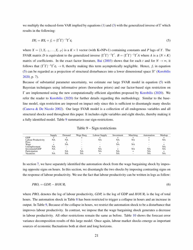
a fully identified model. Table 9 summarizes our sign-restrictions.


Supply Demand Wage Barg. Labour Supply Investment Matching Automation MarkupGDP + + + + + + + +Labour Productivity NA NA - NA NA NA + NAPrice - + - - + - - -Wage + NA - - NA NA - +Unemployment NA - - + - - - NAInvestment/GDP NA - + NA + NA NA NAParticipation - NA NA NA NA + NA +Vacancies NA NA NA + NA - NA NA

In section 7, we have separately identified the automation shock from the wage bargaining shock by impos-

ing opposite signs on hours. In this section, we disentangle the two shocks by imposing contrasting signs on

the response of labour productivity. We use the fact that labour productivity can be written in logs as follow:

PROt = GDPt −HOURt (6)

where PROt denotes the log of labour productivity, GDPt is the log of GDP and HOURt is the log of total

hours. The automation shock in Table 8 has been restricted to trigger a collapse in hours and an increase in

output. In Table 9, Because of the collapse in hours, we restrict the automation shock to be a disturbance that

improves labour productivity. In contrast, we impose that the wage bargaining shock generates a decrease

in labour productivity. All other restrictions remain the same as before. Table 10 shows the forecast error

variance decomposition results of this large model. Once again, labour market shocks emerge as important

sources of economic fluctuations both at short and long horizons.

21

The wage bargaining and labour supply shocks account for the largest share of output, investment and labour

market fluctuations across horizons. The matching efficiency and automation shocks contribute marginally

to business cycle fluctuations but they explain altogether a quite sizable fraction of labour productivity, real

wages and vacancies fluctuations. The supply and investment shocks remain significant drivers of economic

fluctuations. The contribution of the price markup to economic fluctuations is limited in this specification.

Figures 12-13 show the impulses responses to the labour supply and the wage bargaining shock respectively.

The impulse responses of macroeconomic dynamics from the two shocks are statistically significant.

Table 10 – Median Forecast Error Variance Decomposition for the Large Model

Horizon Supply Demand Wage Barg. Lab Supply Investment Matching Automation Markup

GDP 1 0.09 0.02 0.26 0.40 0.08 0.06 0.04 0.045 0.13 0.02 0.27 0.35 0.09 0.05 0.03 0.05

20 0.14 0.02 0.21 0.32 0.13 0.06 0.04 0.07

Labour Productivity 1 0.01 0.08 0.23 0.11 0.42 0.02 0.14 0.005 0.01 0.11 0.31 0.25 0.31 0.00 0.02 0.00

20 0.02 0.09 0.34 0.28 0.23 0.02 0.01 0.01

Prices 1 0.27 0.11 0.12 0.07 0.14 0.09 0.12 0.085 0.24 0.12 0.18 0.07 0.14 0.08 0.10 0.08

20 0.17 0.10 0.33 0.11 0.11 0.05 0.08 0.06

Wages 1 0.12 0.10 0.15 0.30 0.03 0.05 0.14 0.115 0.13 0.10 0.15 0.29 0.04 0.07 0.12 0.11

20 0.06 0.07 0.24 0.22 0.06 0.07 0.19 0.09

Unemployment 1 0.40 0.04 0.33 0.14 0.02 0.02 0.04 0.015 0.44 0.02 0.35 0.05 0.06 0.05 0.02 0.02

20 0.29 0.04 0.23 0.09 0.22 0.04 0.05 0.04

Investment 1 0.19 0.02 0.40 0.22 0.12 0.04 0.01 0.025 0.22 0.01 0.39 0.18 0.12 0.05 0.01 0.02

20 0.16 0.04 0.29 0.20 0.23 0.03 0.03 0.03

Participation 1 0.32 0.02 0.17 0.38 0.03 0.02 0.02 0.055 0.34 0.01 0.13 0.42 0.05 0.01 0.01 0.03

20 0.34 0.01 0.23 0.34 0.04 0.01 0.01 0.03

Vacancies 1 0.00 0.09 0.31 0.33 0.08 0.13 0.05 0.015 0.05 0.05 0.36 0.35 0.09 0.05 0.05 0.01

20 0.11 0.04 0.26 0.39 0.10 0.04 0.05 0.02

9 Conclusion

We apply a structural VAR with sign restriction identification to disentangle supply, demand, and labour

market shocks and to quantify their relevance for economic fluctuations. We estimate our model on Italy’s

data with Bayesian techniques. Given promising labour market trends on labour force participation and

job matching efficiency, we identify shocks that capture these changes and we evaluate their significance

for labour market fluctuations. Our results are as follows. First, we confirm that wage bargaining and

labour supply shocks are among the largest drivers of economic fluctuations both at short and long horizons.

Second, matching efficiency shock and automation shocks are significant drivers of labour market dynamics

but have limited role for output. Third, productivity, demand and investment shocks are also important

contributors of economic and labour market volatility. Our results are consistent with Foroni, Furlanetto &

Lepetit (2018) and Di Giorgio & Giannini (2012) who confirm that the primacy of labour market shocks.

Our findings have appealing policy implications. First, given the burgeoning role of labour market shocks,

we suggest that reforms aimed at improving the flexibility of Italy’s labour market should be strengthened.

22

Second, since investment and labour market shocks explain a lion’s share of labour productivity fluctuations,

we urge policymakers to create favourable conditions that help to stimulate both domestic investment and

marginal efficiency of investment as the latter contributes to improving labour productivity (Justiniano et al.

2010). Third, our results attribute the slowdown in labour productivity growth to a mix of factors including

the lack of adequate investment in R&D activities by Italian firms and stringent labour market policies.

23

References

Acemoglu, D. & Restrepo, P. (2017a), ‘Robots and jobs: Evidence from the us’, NBER Working Paper No

23285.

Acemoglu, D. & Restrepo, P. (2017b), ‘Secular stagnation? the effect of aging on economic growth in the

age of automation’, American Economic Review 107(5), 174–79.

Adda, J., Monti, P., Pellizzari, M., Schivardi, F. & Trigari, A. (2017), ‘Unemployment and skill mismatch in

the italian labour market’. IGIER Bocconi.

Andolfatto, D. (1996), ‘Business cycles and labor-market search’, The american economic review pp. 112–

132.

Arseneau, D. M. & Chugh, S. K. (2012), ‘Tax smoothing in frictional labor markets’, Journal of Political

Economy 120(5), 926–985.

Bai, J. (2003), ‘Inferential theory for factor models of large dimensions’, Econometrica 71(1), 135–171.

Baumeister, C. & Peersman, G. (2013), ‘Time-varying effects of oil supply shocks on the us economy’,

American Economic Journal: Macroeconomics 5(4), 1–28.

Benati, L. & Lubik, T. A. (2014), The time-varying beveridge curve, in ‘Advances in Non-linear Economic

Modeling’, Springer, pp. 167–204.

Berg, A., Buffie, E. F. & Zanna, L.-F. (2018), ‘Should we fear the robot revolution?(the correct answer is

yes)’, Journal of Monetary Economics 97, 117–148.

Bergholt, D., Furlanetto, F. & Faccioli, N. M. (2019), The decline of the labor share: new empirical evi-

dence, Norges Bank.

Blanchard, O. J. & Quah, D. (1989), ‘The dynamic effects of aggregate demand and aggregate supply’, The

American Economic Review 79(4), 655–73.

Brandolini, A., Casadio, P., Cipollone, P., Magnani, M., Rosolia, A. & Torrini, R. (2007), Employment

growth in italy in the 1990s: institutional arrangements and market forces, in ‘Social pacts, employment

and growth’, Springer, pp. 31–68.

Brückner, M. & Pappa, E. (2012), ‘Fiscal expansions, unemployment, and labor force participation: Theory

and evidence’, International Economic Review 53(4), 1205–1228.

Caldara, D., Fuentes-Albero, C., Gilchrist, S. & Zakrajšek, E. (2016), ‘The macroeconomic impact of finan-

cial and uncertainty shocks’, European Economic Review 88, 185–207.

24

Canova, F. & De Nicolo, G. (2002), ‘Monetary disturbances matter for business fluctuations in the g-7’,

Journal of Monetary Economics 49(6), 1131–1159.

Canova, F. & Paustian, M. (2011), ‘Business cycle measurement with some theory’, Journal of Monetary

Economics 58(4), 345–361.

Cantore, C., Ferroni, F. & Leon-Ledesma, M. A. (2017), ‘The dynamics of hours worked and technology’,

Journal of Economic Dynamics and Control 82, 67–82.

Chang, Y. & Schorfheide, F. (2003), ‘Labor-supply shifts and economic fluctuations’, Journal of Monetary

economics 50(8), 1751–1768.

Christiano, L. J., Eichenbaum, M. S. & Trabandt, M. (2016), ‘Unemployment and business cycles’, Econo-

metrica 84(4), 1523–1569.

Christiano, L. J., Eichenbaum, M. & Vigfusson, R. (2004), ‘The response of hours to a technology shock:

Evidence based on direct measures of technology’, Journal of the European Economic Association 2(2-

3), 381–395.

Christiano, L. J., Trabandt, M. & Walentin, K. (2010), Involuntary unemployment and the business cycle,

Technical report, National Bureau of Economic Research.

Ciccarone, G., Dente, G. & Rosini, S. (2016), ‘Labour market and social policy in italy: challenges and

changes’, Sim Europe. Policy Brief 2016/02.

Cirillo, V., Fana, M. & Guarascio, D. (2017), ‘Labour market reforms in italy: evaluating the effects of the

jobs act’, Economia Politica 34(2), 211–232.

Dauth, W., Findeisen, S., Suedekum, J., Woessner, N. et al. (2018), ‘Adjusting to robots: Worker-level

evidence’, Opportunity and Inclusive Growth Institute Working Papers 13.

Daveri, F., Jona-Lasinio, C. & Zollino, F. (2005), ‘Italy’s decline: Getting the facts right [with discussion]’,

Giornale degli economisti e annali di economia pp. 365–421.

De Philippis, M. (2017), ‘The dynamics of the italian labour force participation rate: determinants and

implications for the employment and unemployment rate’, Bank of Italy Occasional Paper (396).

Di Giorgio, C. & Giannini, M. (2012), ‘A comparison of the beveridge curve dynamics in italy and usa’,

Empirical Economics 43(3), 945–983.

Diamond, P. & Blanchard, O. (1989), ‘The beveridge curve’, Brookings Papers on Economic Activity 1, 1–

76.

Dottori, D. (2020), ‘Robots and employment: evidence from italy’, Bank of Italy Occasional Paper (572).

25

European Commission (2006), European trend chart on innovation. country report, italy., Technical report,

Enterprise Directorate-General.

Faust, J. (1998), The robustness of identified var conclusions about money, in ‘Carnegie-Rochester Confer-

ence Series on Public Policy’, Vol. 49, Elsevier, pp. 207–244.

Fisher, J. D. (2006), ‘The dynamic effects of neutral and investment-specific technology shocks’, Journal of

political Economy 114(3), 413–451.

Forni, L., Gerali, A. & Pisani, M. (2010), ‘Macroeconomic effects of greater competition in the service

sector: The case of italy’, Macroeconomic Dynamics 14(5), 677.

Foroni, C., Furlanetto, F. & Lepetit, A. (2018), ‘Labor supply factors and economic fluctuations’, Interna-

tional Economic Review 59(3), 1491–1510.

Francis, N. & Ramey, V. A. (2005), ‘Is the technology-driven real business cycle hypothesis dead? shocks

and aggregate fluctuations revisited’, Journal of Monetary Economics 52(8), 1379–1399.

Fry, R. & Pagan, A. (2011), ‘Sign restrictions in structural vector autoregressions: A critical review’, Journal

of Economic Literature 49(4), 938–60.

Fueki, T., Maehashi, K. et al. (2019), Inflation dynamics in the age of robots: Evidence and some theory,

Technical report, Bank of Japan.

Fujita, S. (2011), ‘Dynamics of worker flows and vacancies: evidence from the sign restriction approach’,

Journal of Applied Econometrics 26(1), 89–121.

Furlanetto, F. & Groshenny, N. (2016), ‘Mismatch shocks and unemployment during the great recession’,

Journal of Applied Econometrics 31(7), 1197–1214.

Furlanetto, F., Ravazzolo, F. & Sarferaz, S. (2019), ‘Identification of financial factors in economic fluctua-

tions’, The Economic Journal 129(617), 311–337.

Furlanetto, F. & Robstad, Ø. (2019), ‘Immigration and the macroeconomy: Some new empirical evidence’,

Review of Economic Dynamics 34, 1–19.

Gali, J. (1999), ‘Technology, employment, and the business cycle: do technology shocks explain aggregate

fluctuations?’, American economic review 89(1), 249–271.

Gali, J. (2011), ‘Monetary policy and unemployment, chapter 10, handbook of monetary economics, volume

3a’.

Galí, J. & Gambetti, L. (2009), ‘On the sources of the great moderation’, American Economic Journal:

Macroeconomics 1(1), 26–57.

26

Galí, J., Smets, F. & Wouters, R. (2012), ‘Unemployment in an estimated new keynesian model’, NBER

macroeconomics annual 26(1), 329–360.

Gambetti, L. (2006), Technology shocks and the response of hours worked: time-varying dynamics matter,

Università degli studi di Modena e Reggio Emilia, Dipartimento di Economia . . . .

Gambetti, L. & Musso, A. (2017), ‘Loan supply shocks and the business cycle’, Journal of Applied Econo-

metrics 32(4), 764–782.

Gambetti, L. & Pistoresi, B. (2004), ‘Policy matters. the long run effects of aggregate demand and mark-up

shocks on the italian unemployment rate’, Empirical Economics 29(2), 209–226.

Gavosto, A. & Pellegrini, G. (1999), ‘Demand and supply shocks in italy:: An application to industrial

output’, European Economic Review 43(9), 1679–1703.

Gerali, A., Locarno, A., Notarpietro, A. & Pisani, M. (2018), ‘The sovereign crisis and italy’s potential

output’, Journal of Policy Modeling 40(2), 418–433.

Hall, B. H., Lotti, F. & Mairesse, J. (2009), ‘Innovation and productivity in smes: empirical evidence for

italy’, Small Business Economics 33(1), 13–33.

IFR (2020), World robotics industrial robots 2020, Technical report, International Federation of Robotics.

Inoue, A. & Kilian, L. (2013), ‘Inference on impulse response functions in structural var models’, Journal

of Econometrics 177(1), 1–13.

Justiniano, A., Primiceri, G. E. & Tambalotti, A. (2010), ‘Investment shocks and business cycles’, Journal

of Monetary Economics 57(2), 132–145.

Justiniano, A., Primiceri, G. E. & Tambalotti, A. (2013), ‘Is there a trade-off between inflation and output

stabilization?’, American Economic Journal: Macroeconomics 5(2), 1–31.

Kilian, L. & Murphy, D. P. (2012), ‘Why agnostic sign restrictions are not enough: understanding the

dynamics of oil market var models’, Journal of the European Economic Association 10(5), 1166–1188.

Korobilis, D. (2020), ‘A new algorithm for sign restrictions in vector autoregressions’, Available at SSRN .

Leduc, S. & Liu, Z. (2020), Robots or workers? a macro analysis of automation and labor markets, Federal

Reserve Bank of San Francisco.

Mountford, A. & Uhlig, H. (2009), ‘What are the effects of fiscal policy shocks?’, Journal of applied

econometrics 24(6), 960–992.

Pappa, E. (2009), ‘The effects of fiscal shocks on employment and the real wage’, International Economic

Review 50(1), 217–244.

27

Peersman, G. (2005), ‘What caused the early millennium slowdown? evidence based on vector autoregres-

sions’, Journal of Applied Econometrics 20(2), 185–207.

Peersman, G. & Straub, R. (2009), ‘Technology shocks and robust sign restrictions in a euro area svar’,

International Economic Review 50(3), 727–750.

Pianta, M. & Vaona, A. (2007), ‘Innovation and productivity in european industries’, Economics of Innova-

tion and New Technology 16(7), 485–499.

Pinelli, D., Torre, R., Pace, L., Cassio, L., Arpaia, A. et al. (2017), The recent reform of the labour market

in italy: A review, Technical report, Directorate General Economic and Financial Affairs (DG ECFIN),

European Commission.

Rubio-Ramirez, J. F., Waggoner, D. F. & Zha, T. (2010), ‘Structural vector autoregressions: Theory of

identification and algorithms for inference’, The Review of Economic Studies 77(2), 665–696.

Schrader, K. & Ulivelli, M. (2017), Italy: A crisis country of tomorrow? insights from the italian labor

market, Technical report, Kiel Policy Brief.

Sims, C. A., Stock, J. H., Watson, M. W. et al. (1990), ‘Inference in linear time series models with some

unit roots’, Econometrica 58(1), 113–144.

Tuzemen, D. & Van Zandweghe, W. (2018), ‘The cyclical behavior of labor force participation’, Federal

Reserve Bank of Kansas City Working Paper No. RWP pp. 18–08.

Uhlig, H. (2005), ‘What are the effects of monetary policy on output? results from an agnostic identification

procedure’, Journal of Monetary Economics 52(2), 381–419.

Zhang, J. (2017), ‘Unemployment benefits and matching efficiency in an estimated DSGE model with labor

market search frictions’, Macroeconomic Dynamics 21(8), 2033–2069.

28

Table 11 – Median Forecast Error Variance Decomposition for the Model Including Hours


GDP 1 0.16 0.09 0.24 0.33 0.175 0.31 0.04 0.15 0.37 0.12

20 0.29 0.11 0.16 0.24 0.21

Hours 1 0.10 0.24 0.11 0.09 0.465 0.14 0.09 0.13 0.26 0.38

20 0.21 0.10 0.12 0.18 0.39

Prices 1 0.27 0.15 0.33 0.10 0.145 0.23 0.19 0.22 0.09 0.27

20 0.20 0.18 0.25 0.11 0.26

Wages 1 0.33 0.19 0.17 0.30 0.005 0.30 0.04 0.10 0.55 0.01

20 0.14 0.17 0.17 0.23 0.29

Unemployment 1 0.07 0.16 0.33 0.31 0.135 0.42 0.06 0.19 0.08 0.25

20 0.27 0.05 0.09 0.05 0.55

Investment 1 0.14 0.05 0.32 0.06 0.435 0.37 0.05 0.20 0.15 0.24

20 0.27 0.06 0.10 0.10 0.48

Table 12 – Median Forecast Error Variance Decomposition Including High-Skill Unemployment


GDP 1 0.16 0.08 0.25 0.40 0.125 0.32 0.04 0.14 0.43 0.07

20 0.25 0.08 0.40 0.19 0.07

Labour Productivity 1 0.08 0.09 0.10 0.00 0.725 0.06 0.09 0.15 0.23 0.47

20 0.21 0.12 0.12 0.26 0.29

Prices 1 0.26 0.10 0.41 0.11 0.125 0.31 0.12 0.25 0.12 0.21

20 0.25 0.11 0.25 0.23 0.16

Wages 1 0.22 0.28 0.25 0.29 0.015 0.16 0.20 0.23 0.27 0.14

20 0.10 0.13 0.46 0.21 0.11

Unemployment-High Skill 1 0.01 0.21 0.33 0.32 0.125 0.15 0.15 0.40 0.19 0.11

20 0.25 0.09 0.43 0.14 0.10

Investment 1 0.16 0.07 0.30 0.06 0.405 0.38 0.08 0.18 0.20 0.15

20 0.30 0.08 0.34 0.13 0.15

29

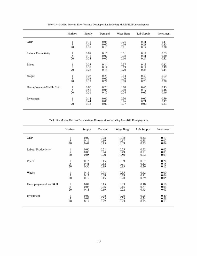
Table 13 – Median Forecast Error Variance Decomposition Including Middle-Skill Unemployment


GDP 1 0.15 0.08 0.25 0.41 0.115 0.37 0.07 0.16 0.28 0.1320 0.31 0.13 0.11 0.17 0.28


Prices 1 0.25 0.14 0.37 0.13 0.125 0.35 0.14 0.19 0.14 0.1920 0.26 0.14 0.20 0.26 0.14

Wages 1 0.28 0.26 0.14 0.30 0.025 0.38 0.07 0.06 0.47 0.0120 0.17 0.27 0.08 0.20 0.28

Unemployment-Middle Skill 1 0.00 0.20 0.20 0.46 0.135 0.51 0.06 0.10 0.17 0.1620 0.31 0.15 0.04 0.05 0.46

Investment 1 0.14 0.09 0.30 0.09 0.395 0.44 0.03 0.16 0.21 0.1720 0.32 0.09 0.07 0.09 0.43

Table 14 – Median Forecast Error Variance Decomposition Including Low-Skill Unemployment


GDP 1 0.09 0.28 0.08 0.42 0.135 0.19 0.19 0.17 0.38 0.07

20 0.47 0.15 0.09 0.25 0.04


20 0.05 0.20 0.50 0.22 0.03

Prices 1 0.15 0.15 0.39 0.07 0.245 0.41 0.12 0.21 0.12 0.15

20 0.30 0.19 0.13 0.26 0.12

Wages 1 0.15 0.08 0.35 0.42 0.005 0.17 0.09 0.29 0.41 0.04

20 0.12 0.15 0.28 0.39 0.05

Unemployment-Low Skill 1 0.02 0.15 0.33 0.40 0.105 0.08 0.06 0.15 0.67 0.04

20 0.11 0.19 0.22 0.43 0.05

Investment 1 0.07 0.02 0.26 0.25 0.405 0.09 0.23 0.23 0.24 0.21

20 0.12 0.27 0.23 0.25 0.13

30

Table 15 – Median Forecast Error Variance Decomposition Including Men Unemployment


GDP 1 0.13 0.08 0.23 0.41 0.155 0.31 0.04 0.18 0.34 0.13

20 0.29 0.11 0.13 0.19 0.28


20 0.12 0.11 0.19 0.11 0.47

Prices 1 0.30 0.14 0.36 0.08 0.125 0.22 0.22 0.19 0.09 0.29

20 0.18 0.20 0.21 0.12 0.28

Wages 1 0.32 0.21 0.19 0.28 0.005 0.35 0.07 0.13 0.45 0.01

20 0.14 0.19 0.16 0.16 0.36

Unemployment-Men 1 0.06 0.13 0.31 0.35 0.145 0.42 0.06 0.18 0.04 0.30

20 0.23 0.14 0.07 0.02 0.53

Investment 1 0.15 0.04 0.31 0.12 0.395 0.36 0.03 0.22 0.16 0.23

20 0.25 0.10 0.11 0.06 0.48

Table 16 – Median Forecast Error Variance Decomposition Including Women Unemployment


GDP 1 0.15 0.10 0.27 0.30 0.185 0.34 0.04 0.10 0.39 0.12

20 0.25 0.08 0.33 0.20 0.14


20 0.17 0.09 0.09 0.19 0.45

Prices 1 0.26 0.11 0.39 0.11 0.135 0.24 0.14 0.29 0.08 0.24

20 0.21 0.16 0.25 0.13 0.24

Wages 1 0.21 0.27 0.19 0.32 0.005 0.18 0.09 0.18 0.52 0.03

20 0.11 0.14 0.35 0.26 0.14

Unemployment-Women 1 0.04 0.13 0.44 0.27 0.125 0.36 0.08 0.23 0.14 0.19

20 0.27 0.05 0.32 0.10 0.25

Investment 1 0.11 0.04 0.30 0.03 0.515 0.39 0.05 0.13 0.15 0.27

20 0.26 0.05 0.25 0.10 0.33

31

Table 17 – Median Forecast Error Variance Decomposition Including Two Lags


GDP 1 0.10 0.25 0.09 0.43 0.135 0.12 0.28 0.07 0.44 0.0920 0.26 0.32 0.05 0.20 0.17


Prices 1 0.20 0.37 0.30 0.07 0.065 0.19 0.36 0.27 0.12 0.0620 0.11 0.32 0.18 0.35 0.04

Wages 1 0.25 0.09 0.23 0.43 0.005 0.14 0.01 0.13 0.70 0.0320 0.13 0.01 0.10 0.69 0.07

Unemployment 1 0.02 0.09 0.14 0.67 0.075 0.06 0.04 0.02 0.83 0.0520 0.10 0.02 0.02 0.79 0.07

Investment 1 0.23 0.15 0.24 0.25 0.135 0.25 0.14 0.23 0.25 0.1320 0.23 0.13 0.23 0.28 0.13

Table 18 – Median Forecast Error Variance Decomposition Including Large Sample


GDP 1 0.40 0.14 0.10 0.26 0.105 0.64 0.15 0.10 0.08 0.0320 0.34 0.43 0.15 0.08 0.01


Prices 1 0.30 0.12 0.32 0.13 0.135 0.32 0.13 0.31 0.12 0.1220 0.24 0.20 0.36 0.10 0.09

Wages 1 0.64 0.05 0.15 0.14 0.025 0.43 0.06 0.38 0.03 0.1120 0.30 0.22 0.36 0.04 0.08

Unemployment 1 0.05 0.18 0.39 0.24 0.135 0.05 0.27 0.19 0.24 0.2420 0.25 0.58 0.03 0.09 0.05

Investment 1 0.01 0.30 0.34 0.04 0.315 0.26 0.31 0.23 0.08 0.1420 0.21 0.61 0.05 0.11 0.03

32

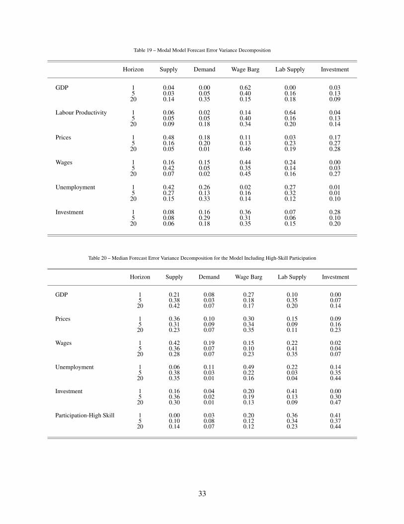
Table 19 – Modal Model Forecast Error Variance Decomposition


GDP 1 0.04 0.00 0.62 0.00 0.035 0.03 0.05 0.40 0.16 0.1320 0.14 0.35 0.15 0.18 0.09


Prices 1 0.48 0.18 0.11 0.03 0.175 0.16 0.20 0.13 0.23 0.2720 0.05 0.01 0.46 0.19 0.28

Wages 1 0.16 0.15 0.44 0.24 0.005 0.42 0.05 0.35 0.14 0.0320 0.07 0.02 0.45 0.16 0.27

Unemployment 1 0.42 0.26 0.02 0.27 0.015 0.27 0.13 0.16 0.32 0.0120 0.15 0.33 0.14 0.12 0.10

Investment 1 0.08 0.16 0.36 0.07 0.285 0.08 0.29 0.31 0.06 0.1020 0.06 0.18 0.35 0.15 0.20

Table 20 – Median Forecast Error Variance Decomposition for the Model Including High-Skill Participation


GDP 1 0.21 0.08 0.27 0.10 0.005 0.38 0.03 0.18 0.35 0.07

20 0.42 0.07 0.17 0.20 0.14

Prices 1 0.36 0.10 0.30 0.15 0.095 0.31 0.09 0.34 0.09 0.16

20 0.23 0.07 0.35 0.11 0.23

Wages 1 0.42 0.19 0.15 0.22 0.025 0.36 0.07 0.10 0.41 0.04

20 0.28 0.07 0.23 0.35 0.07

Unemployment 1 0.06 0.11 0.49 0.22 0.145 0.38 0.03 0.22 0.03 0.35

20 0.35 0.01 0.16 0.04 0.44

Investment 1 0.16 0.04 0.20 0.41 0.005 0.36 0.02 0.19 0.13 0.30

20 0.30 0.01 0.13 0.09 0.47

Participation-High Skill 1 0.00 0.03 0.20 0.36 0.415 0.10 0.08 0.12 0.34 0.37

20 0.14 0.07 0.12 0.23 0.44

33

Table 21 – Median Forecast Error Variance Decomposition for the Model Including Middle Skill-Participation


GDP 1 0.15 0.15 0.24 0.37 0.105 0.12 0.07 0.06 0.60 0.16

20 0.07 0.19 0.26 0.34 0.14

Prices 1 0.31 0.12 0.29 0.20 0.085 0.16 0.29 0.32 0.15 0.08

20 0.09 0.24 0.23 0.15 0.30

Wages 1 0.22 0.07 0.24 0.33 0.145 0.11 0.02 0.43 0.34 0.10

20 0.04 0.32 0.40 0.15 0.09

Unemployment 1 0.02 0.08 0.48 0.32 0.095 0.14 0.05 0.13 0.09 0.60

20 0.05 0.10 0.15 0.11 0.58

Investment 1 0.08 0.11 0.36 0.05 0.405 0.08 0.05 0.08 0.28 0.51

20 0.04 0.08 0.10 0.22 0.56

Participation-Middle Skill 1 0.01 0.31 0.14 0.41 0.135 0.07 0.26 0.20 0.37 0.10

20 0.07 0.22 0.25 0.38 0.09

Table 22 – Median Forecast Error Variance Decomposition for the Model Including Low Skill-Participation


GDP 1 0.19 0.11 0.30 0.27 0.125 0.30 0.05 0.12 0.39 0.1320 0.26 0.06 0.13 0.25 0.29

Prices 1 0.36 0.11 0.33 0.11 0.105 0.26 0.10 0.48 0.08 0.0820 0.24 0.07 0.39 0.12 0.17

Wages 1 0.42 0.12 0.10 0.29 0.085 0.34 0.02 0.09 0.42 0.1320 0.22 0.08 0.32 0.26 0.12

Unemployment 1 0.18 0.10 0.41 0.19 0.135 0.48 0.02 0.28 0.04 0.1820 0.37 0.01 0.16 0.05 0.41

Investment 1 0.14 0.05 0.38 0.00 0.435 0.33 0.02 0.24 0.06 0.3620 0.22 0.01 0.15 0.05 0.56

Participation-Low Skill 1 0.03 0.01 0.34 0.32 0.295 0.20 0.04 0.16 0.38 0.2220 0.29 0.05 0.13 0.28 0.26

34

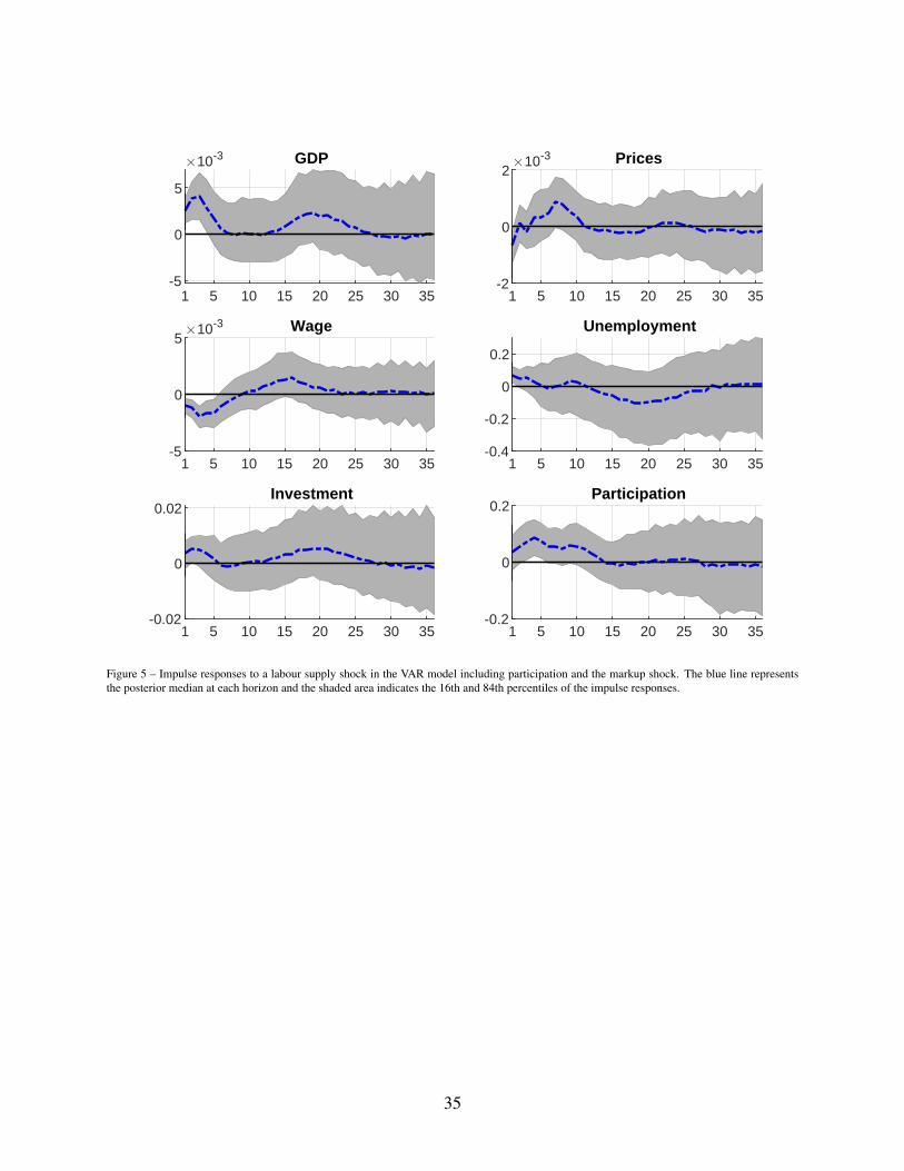
1 5 10 15 20 25 30 35-5

0

5

10-3 GDP

1 5 10 15 20 25 30 35-2

0

210-3 Prices

1 5 10 15 20 25 30 35-5

0

510-3 Wage

1 5 10 15 20 25 30 35-0.4

-0.2

0

0.2

Unemployment

1 5 10 15 20 25 30 35-0.02

0

0.02 Investment

1 5 10 15 20 25 30 35-0.2

0

0.2 Participation

Figure 5 – Impulse responses to a labour supply shock in the VAR model including participation and the markup shock. The blue line representsthe posterior median at each horizon and the shaded area indicates the 16th and 84th percentiles of the impulse responses.

35

1 5 10 15 20 25 30 35-5

0

5

10-3 GDP

1 5 10 15 20 25 30 35

-2

0

210-3 Prices

1 5 10 15 20 25 30 35-5

0

510-3 Wage

1 5 10 15 20 25 30 35

-0.4

-0.2

0

0.2 Unemployment

1 5 10 15 20 25 30 35-0.02

0

0.02

Investment

1 5 10 15 20 25 30 35-0.2

0

0.2 Participation

Figure 6 – Impulse responses to a wage bargaining shock in the VAR model including participation and the markup shock. The blue line representsthe posterior median at each horizon and the shaded area indicates the 16th and 84th percentiles of the impulse responses.

36

1 5 10 15 20 25 30 35-0.01

0

0.01 GDP

1 5 10 15 20 25 30 35

-2

0

2

410-3 Prices

1 5 10 15 20 25 30 35-0.5

0

0.5 Unemployment

1 5 10 15 20 25 30 35-0.1

0

0.1 Vacancies

1 5 10 15 20 25 30 35

-0.02

0

0.02

Investment

1 5 10 15 20 25 30 35-0.2

0

0.2

Participation

Figure 7 – Impulse responses to a labour supply shock in the VAR model including vacancies. The blue line represents the posterior median at eachhorizon and the shaded area indicates the 16th and 84th percentiles of the impulse responses.

37

1 5 10 15 20 25 30 35-0.01

0

0.01

GDP

1 5 10 15 20 25 30 35

-4

-2

0

210-3 Prices

1 5 10 15 20 25 30 35-1

-0.5

0

0.5 Unemployment

1 5 10 15 20 25 30 35

-0.1

0

0.1 Vacancies

1 5 10 15 20 25 30 35-0.05

0

0.05 Investment

1 5 10 15 20 25 30 35-0.4

-0.2

0

0.2 Participation

Figure 8 – Impulse responses to a matching efficiency shock in the VAR model including vacancies. The blue line represents the posterior medianat each horizon and the shaded area indicates the 16th and 84th percentiles of the impulse responses.

38

1 5 10 15 20 25 30 35

-5

0

5

1010-3 GDP

1 5 10 15 20 25 30 35-0.02

0

0.02 Hours

1 5 10 15 20 25 30 35

-2

0

210-3 Prices

1 5 10 15 20 25 30 35

-2

0

2

10-3 Wage

1 5 10 15 20 25 30 35-0.4

-0.2

0

0.2

Unemployment

1 5 10 15 20 25 30 35-0.02

0

0.02 Investment

Figure 9 – Impulse responses to a labour Supply shock in the VAR including hours. The blue line represents the posterior median at each horizonand the shaded area indicates the 16th and 84th percentiles of the impulse responses.

39

1 5 10 15 20 25 30 35-5

0

510-3 GDP

1 5 10 15 20 25 30 35-0.01

0

0.01

Hours

1 5 10 15 20 25 30 35

-2

0

210-3 Prices

1 5 10 15 20 25 30 35-2

0

2

10-3 Wage

1 5 10 15 20 25 30 35

-0.2

0

0.2 Unemployment

1 5 10 15 20 25 30 35-0.01

0

0.01

0.02 Investment

Figure 10 – Impulse responses to a wage bargaining shock in the VAR including hours. The blue line represents the posterior median at each horizonand the shaded area indicates the 16th and 84th percentiles of the impulse responses.

40

1 5 10 15 20 25 30 35-5

0

510-3 GDP

1 5 10 15 20 25 30 35-0.01

0

0.01 Hours

1 5 10 15 20 25 30 35

-2

0

210-3 Prices

1 5 10 15 20 25 30 35

-2

0

210-3 Wage

1 5 10 15 20 25 30 35-0.2

0

0.2 Unemployment

1 5 10 15 20 25 30 35

-0.01

0

0.01 Investment

Figure 11 – Impulse responses to an automation shock in the VAR including hours. The blue line represents the posterior median at each horizonand the shaded area indicates the 16th and 84th percentiles of the impulse responses.

41

GDP

10 20 30-1

0

1

2

3

410-3 Labor Productivity

10 20 30-8

-6

-4

-2

0

2

410-3 Prices

10 20 30-1.5

-1

-0.5

0

0.5

110-3 Wage

10 20 30-2

-1.5

-1

-0.5

0

0.5

1

1.510-3

Unemployment

10 20 30-0.15

-0.1

-0.05

0

0.05

0.1

0.15Investment

10 20 30-2

0

2

4

6

8

1010-3 Participation

10 20 30-0.05

0

0.05

0.1

Responses to an Lab Supply shock

Vacancies

10 20 30-0.02

-0.01

0

0.01

0.02

0.03

0.04

0.05

Figure 12 – Impulse responses to a labour supply shock in the large VAR. The blue line represents the posterior median at each horizon, and the shaded area shows their 90 percent bands.

42

GDP

10 20 30-2

-1

0

1

2

3

410-3 Labor Productivity

10 20 30-8

-6

-4

-2

0

2

410-3 Prices

10 20 30-1.5

-1

-0.5

0

0.5

110-3 Wage

10 20 30-2

-1.5

-1

-0.5

0

0.5

110-3

Unemployment

10 20 30-0.15

-0.1

-0.05

0

0.05Investment

10 20 30-4

-2

0

2

4

6

8

10

1210-3 Participation

10 20 30-0.1

-0.08

-0.06

-0.04

-0.02

0

0.02

Responses to a Wage Barg shock

Vacancies

10 20 30-0.02

-0.01

0

0.01

0.02

0.03

0.04

0.05

Figure 13 – Impulse responses to a wage bargaining shock in the large VAR. The blue line represents the posterior median at each horizon, and the grey shaded area shows their 90 percent bands.

43

A Appendix

A.1 The Model and the Identification Strategy

In this appendix, we explain thoroughly the econometric procedure we apply for the estimation of our model.

We consider the following reduced-form VAR representation:

Yt =CA +P

∑i=1

AiYt−i + εt (7)

where Yt is a (N×1) vector containing all N endogenous variables, CA is a (N×1) vector of constants, Ai

for i = 1, ...,P are (N×N) matrices of parameters. P denotes the number of lags and εt is a (N×1) vector

of reduced form residuals with εt ∼ N (0,Σ) where Σ is the (N×N) variance-covariance matrix. Since

we account for large parameter uncertainty, we use the Bayesian estimation methods to estimate our model

parameters. The model is specified and estimated in level given that Bayesian estimation methods can be

applied irrespective of non-stationarity in data (Sims et al. 1990).

Bayesian Estimation

We can write our model in (7) in seemingly unrelated regression (SUR) representation as follows:

Y = XA+E (8)

where Y = [yp+1 . . .yT ]′, A = [CA A1 . . .Ap]

′, E = [ε1...εT ]

′and

X =

1 y

′0 . . . y

′−p

......

......

1 y′T−1 . . . y

′T−p

By vectorizing (8), we obtain the following:

y = (In⊗X)α + ε (9)

where y = vec(Y ), α = vec(A), ε = vec(E) and vec() denotes columwise vectorization. Given the normality

assumption of the error term ε with a mean zero and variance-covariance Σ⊗ IT−p, the likelihood function

conditional on the parameters of the model α and Σ and the regressors X can be written as follows:

L(y|X ,α,Σ) ∝ |Σ⊗ IT−p|−T−p

2 exp

12(y− In⊗Xα)

′(Σ⊗ IT−p)

−1(y− In⊗Xα)

(10)

where y denotes the available data. Denoting α = vec(A) where A = (X′X)−1X

′Y denotes the OLS estimate

and letting Λ = (Y −XA)′(Y −XA) be the sum of squared errors, then the likelihood function in (10) can be

44

rewritten as follows:

L(y|X ,α,Σ) ∝ |Σ⊗ IT−p|−T−p

2 exp

12(α− α)

′(Σ−1⊗X

′X)(α− α)

exp−1

2tr(Σ−1

Λ)

(11)

We then specify diffuse priors for α and Σ that are proportional to |Σ|− n+12 namely:

p(A|Σ) ∝ 1

p(Σ) ∝ |Σ|−n+1

2

By combining our diffuse priors with the likelihood function using Bayes rule, we then obtain Normal-

Inverse Wishart posterior:

L(α,Σ|y,X) ∝ L(y|X ,α,Σ)p(A|Σ)p(Σ)

= |Σ|−T−p+n+1

2 exp

12(α− α)

′(Σ−1⊗X

′X)(α− α)

exp−1

2tr(Σ−1

Λ)

(12)

The likelihood function in (12) is a product of a normal distribution for α given Σ and an inverse Wishart

distribution for Σ. Thus, we draw α conditional on Σ from

α|Σ,y,X ∼N (α,Σ⊗ (X′X)−1

and Σ from

Σ|y,X ∼I W (Λ,v)

where v = T − p− (np+1)−n−1; I W denotes an inverse-Wishart distribution.

Sign Identification

In order to recover the impact of structural shocks from our reduced-form forecast errors, we assume that

the forecast error εt is a linear combination of structural disturbances ηt such that:

εt = Sηt (13)

where ηt ∼N (0,Ω) denotes the (N×N) variance-covariance matrix of structural form innovations and

Ω = I. The variance-covariance matrix in (13) is given by Σ = SS′. Σ has N(N+1)

2 distinct parameters while

S has N2 independent parameters. Thus, in order to identify structural shocks, we need to impose N(N−1)2

restrictions on S. In the Cholesky decomposition, S is restricted to be lower triangular, thereby implying

a recursive identification procedure. However, in the Cholesky decomposition, the covariance matrix is

assumed as Σ = SINS′

where IN = QQ′

and Q denotes an orthonormal matrix. To obtain identification

through sign restrictions, we need to specify a set of admissible Q matrices (Caldara et al. 2016). To

45

accomplish this task, we follow the procedure proposed by Rubio-Ramirez, Waggoner & Zha (2010). This

procedure works as follows. Firstly, we draw from a MN (0N ,IN) and perform a QR decomposition of

S with the diagonal of R normalized to be positive, where QQ′= IN . Secondly, we impose the Cholesky

decomposition on S such that Σ = SS′ where S denotes a Cholesky factor. We then compute candidate

impulse responses from SQ′and Ai for i = 1, . . . ,P and check if the generated impulse responses satisfy the

sign restrictions or not. If they do satisfy the sign restrictions, store them, otherwise, discard them and return

to the initial step. We repeat the same procedure until we obtain 500 impulse responses which satisfy our

sign restrictions.

A.2 VAR Including Participation


Supply Demand Wage Barg. Lab Supply InvestmentGDP + + + + +Price - + - - +Real Wage + NA - - NAUnemployment NA - - + -Investment/GDP NA - + NA +Participation NA NA - + +

Table 24 – Median Forecast Error Variance Decomposition for the Model Including Participation


GDP 1 0.14 0.12 0.23 0.35 0.165 0.32 0.06 0.11 0.39 0.12

20 0.34 0.10 0.32 0.13 0.07

Prices 1 0.37 0.11 0.32 0.13 0.075 0.28 0.16 0.34 0.08 0.15

20 0.23 0.18 0.27 0.16 0.17

Wages 1 0.31 0.13 0.20 0.33 0.025 0.34 0.03 0.06 0.47 0.09

20 0.20 0.21 0.23 0.30 0.05

Unemployment 1 0.07 0.09 0.51 0.24 0.095 0.41 0.05 0.25 0.06 0.23

20 0.42 0.03 0.11 0.05 0.40

Investment 1 0.07 0.06 0.41 0.04 0.425 0.34 0.05 0.22 0.07 0.33

20 0.28 0.05 0.14 0.04 0.49

Participation 1 0.00 0.06 0.22 0.52 0.195 0.04 0.05 0.10 0.57 0.25

20 0.17 0.09 0.14 0.41 0.20

46

A.3 Data sources

In this subsection, we summarize the data sources for our variables. When the original data series is in an

annual frequency, we transform into a quarterly frequency using the Quadratic-Match Average interpolation

method from Eviews. When the original series is in monthly frequency, we take quarterly averages of

monthly data. All data are seasonally adjusted and expressed in logs except unemployment, vacancies and

participation.

• Output: seasonally adjusted quarterly gross domestic product(GDP) at market prices taken national

accounts, Code namq_10_gd p. Source: Eurostat.

• Prices: seasonally adjusted quarterly GDP deflator computed by taking the change in GDP at market

prices in the current period and GDP in market prices in the previous period multiply by 100. Source:

Istat.

• Real wages: seasonally adjusted quarterly domestic wages and salaries per employee in hours worked

adjusted for harmonised consumer price index (HCPI), base year 2015=100, code prc_hicp_midx.

Sources: Istat and Eurostat. Annual real wages data are converted into quarterly frequencies using

the Quadratic-Match Average method from Eviews 8.

• Hours: seasonally adjusted total hours computed by taking the product of quarterly employment rate

(15-64 years old) in percent of labour force from labour force survey and the volume of work done

(hours worked) industry, base year 2015=100. Sources: Istat and Eurostat.

• Unemployment rate: seasonally adjusted quarterly unemployment rate aged 15-64 out of labour force

from labour force survey. Source: Istat.

• Unemployment by gender: seasonally adjusted quarterly unemployment rate (15-64 years old) out of

labour force from labour force survey. Source: Istat.

• Unemployment rate by education level: quarterly unemployment rate (15-64 years old) out of labour

force from labour force survey, code l f squrgaed. Source: eurostat. It is seasonally adjusted using a

default implementation of X-12 triggered from Demetra 2.2.3.

• Participation rate: seasonally adjusted quarterly activity rate (15-64 years old) from labour force

survey. Source: Istat.

• Participation rate by education level: quarterly activity rate (15-64 years old) from labour force sur-

vey, code l f sqargaed. Source: eurostat. It is seasonally adjusted using a default implementation of

X-12 obtained from Demetra 2.2.3.

• Vacancies: seasonally adjusted quarterly job vacancy rate taken from Istat.

• Investment: seasonally adjusted quarterly gross fixed capital formation, current prices, million euro

taken national accounts, Code namq_10_gd p. Source: Eurostat.

• Labour Productivity: This is computed as the log difference of output and hours.

47

Documents

Josué Diwambuena, Francesco Ravazzolo