ISTANBUL TECHNICAL UNIVERSITY F GRADUATE SCHOOL OF SCIENCE

ENGINEERING AND TECHNOLOGY

DIRAC SYSTEMS IN TERMS OF THE BERRY GAUGE FIELDSAND EFFECTIVE FIELD THEORY OF A TOPOLOGICAL INSULATOR

Ph.D. THESIS

Elif YUNT

Department of Physics Engineering

Physics Engineering Programme

DECEMBER 2014

ISTANBUL TECHNICAL UNIVERSITY F GRADUATE SCHOOL OF SCIENCE

ENGINEERING AND TECHNOLOGY

DIRAC SYSTEMS IN TERMS OF THE BERRY GAUGE FIELDSAND EFFECTIVE FIELD THEORY OF A TOPOLOGICAL INSULATOR

Ph.D. THESIS

Elif YUNT(509062102)

Department of Physics Engineering

Physics Engineering Programme

Thesis Advisor: Prof. Dr. Ömer F. DAYI

DECEMBER 2014

ISTANBUL TEKNIK ÜNIVERSITESI F FEN BILIMLERI ENSTITÜSÜ

BERRY AYAR ALANLARI CINSINDEN DIRAC SISTEMLERIVE BIR TOPOLOJIK YALITKANIN ETKIN ALAN KURAMI

DOKTORA TEZI

Elif YUNT(509062102)

Fizik Mühendisligi Anabilim Dalı

Fizik Mühendisligi Programı

Tez Danısmanı: Prof. Dr. Ömer F. DAYI

ARALIK 2014

Elif YUNT, a Ph.D. student of ITU Graduate School of Science Engineering andTechnology with student ID 509062102 has successfully defended the thesis entitled“DIRAC SYSTEMS IN TERMS OF THE BERRY GAUGE FIELDS AND EF-FECTIVE FIELD THEORY OF A TOPOLOGICAL INSULATOR”, which sheprepared after fulfilling the requirements specified in the associated legislations, beforethe jury whose signatures are below.

Thesis Advisor : Prof. Dr. Ömer F. DAYI ..............................Istanbul Technical University

Jury Members : Assoc. Prof. Dr. Ali Yıldız ..............................Istanbul Technical University

Assoc. Prof . Dr. Levent Subası ..............................Istanbul Technical University

Prof. Dr. Ersan Demiralp ..............................Bogaziçi University

Prof. Dr. Kayhan Ülker ..............................Mimar Sinan Fine Arts University

Date of Submission : 24 November 2014Date of Defense : 12 December 2014

v

vi

FOREWORD

I would like to thank my supervisor, Prof. Dr. Ömer Faruk Dayı who has agreed toteach me and encouraged me all throughout this long period of research with his raresense of responsibility and respect for his profession and the student. I would like tothank my family who have not only inspired me for higher education but also tookpride in my work, supporting all along patiently. I would like to thank all contributorsof the so-called Fizik Haftaları which took place through the span of last five yearsproviding me the opportunity to communicate to dozens of physicists, to teach physicsand to discuss physics, for the inspiration. I would like to dedicate this thesis to all intheir naive pursuit of understanding existence through science, especially to all womenin this pursuit in the hope that they have faith in their authentic merits and eventuallybring them more and more to the science arena.

December 2014 Elif YUNT

vii

viii

TABLE OF CONTENTS

Page

FOREWORD........................................................................................................... viiTABLE OF CONTENTS........................................................................................ ixABBREVIATIONS ................................................................................................. xiLIST OF FIGURES ................................................................................................ xiiiSUMMARY ............................................................................................................. xvÖZET .......................................................................................................................xvii1. INTRODUCTION .............................................................................................. 12. DIRAC HAMILTONIAN, FOLDY-WOUTHUYSEN TRANSFORMA-TION, AND THE BERRY GAUGE FIELDS IN D-DIMENSIONS.................. 7

2.1 Derivation of Dirac Hamiltonian on graphene à la Semenoff ........................ 82.2 Derivation of Dirac Hamiltonian on graphene à la Novoselov et al............... 112.3 Derivation of Dirac Hamiltonian on graphene à la Gusynin et al .................. 132.4 Foldy-Wouthuysen transformation and Berry gauge fields ............................ 16

3. RELATION BETWEEN THE SPIN HALL CONDUCTIVITY AND THESPIN CHERN NUMBER FOR DIRAC-LIKE SYSTEMS................................. 19

3.1 Wave-packet dynamics ................................................................................... 213.2 Semiclassical formalism................................................................................. 243.3 Anomalous Hall effect.................................................................................... 273.4 Spin Hall conductivity vs spin Chern number................................................ 283.5 Kane-Mele Model........................................................................................... 293.6 Kane-Mele model without the Rashba spin-orbit interaction term ............... 303.7 Kane-Mele model with Rashba spin-orbit interaction term ........................... 34

4. EFFECTIVE FIELD THEORY OF TIME-REVERSAL INVARIANTTOPOLOGICAL INSULATORS.......................................................................... 37

4.1 2+1 Dimensional topological insulator and dimensional reduction to 1+1dimension ...................................................................................................... 37

4.1.1 A model for 2+1-dimensional topological insulator ........................... 394.1.2 Dimensional reduction to 1+1 dimensions .......................................... 41

4.2 4+1 Dimensional topological insulator and dimensional reduction to 3+1and 2+1 dimensions ....................................................................................... 43

4.2.1 Dimensional reduction to 3+1 dimensions .......................................... 444.2.2 A hypothetical model for 3+1 dimensional topological insulators ..... 464.2.3 Dimensional reduction to 2+1-dimensions........................................... 48

5. CONCLUSIONS................................................................................................. 51REFERENCES........................................................................................................ 53APPENDICES......................................................................................................... 59

APPENDIX A : Kubo Formula Derivation of Spin Hall Conductivity................ 61

ix

APPENDIX B : Berry Gauge Field and Curvature in 4+1 Dimensions............. 63APPENDIX C : Eigenstates of Kane-Mele Hamiltonian in the Presence of

Spin-orbit Coupling ....................................................................................... 64CURRICULUM VITAE......................................................................................... 65

x

ABBREVIATIONS

TRI : Time Reversal InvariantSO : Spin-OrbitSOI : Spin-Orbit InteractionTRB : Time Reversal BreakingQHE : Quantum Hall EffectSQHE : Spin Quantum Hall Effect

xi

xii

LIST OF FIGURES

Page

Figure 2.1 : Honeycomb lattice 1. ........................................................................ 8Figure 2.2 : Brillouin zone 1 and degeneracy points............................................ 9Figure 2.3 : Honeycomb lattice 2. ........................................................................ 11Figure 2.4 : Brillouin zone 2 and degeneracy points............................................ 12Figure 2.5 : Honeycomb lattice 3. ........................................................................ 14Figure 2.6 : Brillouin zone 3 and degeneracy points............................................ 14

xiii

xiv

DIRAC SYSTEMS IN TERMS OF THE BERRY GAUGE FIELDSAND EFFECTIVE FIELD THEORY OF A TOPOLOGICAL INSULATOR

SUMMARY

Dirac systems in terms the of Berry gauge fields and the effective field theory ofa time-reversal invariant topological insulator are investigated. Dirac systems orDirac-like systems are non-relativistic systems, e.g. condensed matter systems, wherethe description of the physical system is given by either the massive or masslessDirac Hamiltonian. The Dirac systems investigated in this thesis are the time-reversalinvariant topological insulators. A topological insulator is a bulk insulator withconducting edge states characterized by a topological number. The first theoreticalmodel of the time-reversal invariant topological insulators is the Kane-Mele modelof graphene where the intrinsic spin-orbit interaction and time-reversal symmetry ispredicted to cause a quantized spin Hall current at the edges , leading to a quantizedspin Hall conductivity given by the the topological Chern number.As the theoretical background, the explicit derivation of 2+ 1 dimensional masslessDirac Hamiltonian on graphene is given. The Berry gauge field and the correspondingBerry curvature are defined for massive free Dirac Hamiltonian in arbitrary dimensionsemploying the Foldy-Wouthuysen transformation of the Dirac Hamiltonian. Thedefinitions of the first and second Chern numbers in terms of Berry curvature are given.In the first part of the thesis, a semiclassical formulation of the quantum spin Halleffect for physical systems satisfying Dirac-like equation is introduced. Quantumspin Hall effect is essentially a phenomenon in two space dimensions. In thesemiclassical formulation adopted in the thesis, the position and momenta are classicalphase space variables, and spin is not considered as a dynamical degree of freedom.The derivation of the matrix-valued one-form lying at the heart of the semiclassicalformulation adopted is made explictly using a wave-packet constructed from thepositive energy eigenstates of free Dirac equation. Defining the symplectic two-formand employing Liouville equation, the semiclassical matrix-valued equations of motionare obtained. The phase space measure, w1/2, and time evolutions of phase spacevariables, ˙xiw1/2 and ˙piw1/2, are obtained in terms of the phase space variables. As anintroductory example, the formalism is displayed through the anamolous Hall effect.The anamolous Hall conductivity is established from the term linear in the electricfield and the Berry curvature in ˙xiw1/2. The semiclassical formulation adopted is thenillustrated within the Kane-Mele model of graphene in the absence and in the presenceof the Rashba spin-orbit coupling term. The spin Hall current is defined with the aidof the equations for the time evolutions of phase space variables in terms of phasespace variables. The spin Hall conductivity is established from the term linear inthe elctric field and the Berry curvature in ˙xiw1/2. It is shown that if one adopts thecorrect definition of the spin current in two space dimensions, the essential part ofthe spin Hall conductivity is always given by the spin Chern number whether thespin is conserved or not at the quantum level. In the absence of Rashba spin-orbitcoupling, the third component of spin is conserved, and the definition of the spin Hall

xv

current is straightforward. In the presence of Rashba spin-orbit coupling, the thirdcomponent of spin is not conserved so that a suitable base of spin eigenstates needto be employed to define spin Hall current. The anomalous velocity term survives inany d+1 spacetime dimension, since independent of the spacetime dimension and theorigin of the Berry curvature in the time evolution of the coordinates there is alwaysa term which is linear in both electric field and the Berry field strength. In the basiswhere a certain component of spin is diagonal this term will be diagonal.In the second part of the thesis, a field theoretic investigation of topological insulatorsin 2+ 1 and 4+ 1 dimensions is presented using Chern-Simons theory and a methodof dimensional reduction. Chern-Simons actions emerge as the effective field theoriesfrom the actions describing Dirac fermions in the presence of external gauge fields. Atime-reversal invariant topological insulator model in 2+1 dimensions is discussed andby means of a dimensional reduction the 1+ 1 dimensional descendant is presented.The field strength of the Berry gauge field corresponding to the 4+ 1 dimensionalDirac theory is explicitly derived through the Foldy-Wouthuysen transformation.Acquainted with it, the second Chern number is calculated for specific choices ofthe integration domain. The Foldy-Wouthuysen transformation which diagonalizesthe Dirac Hamiltonian is proven to be a powerful tool to perform calculations inthe effective field theory of the 4+ 1 dimensional time-reversal invariant topologicalinsulator. A method is proposed to obtain 3+1 and 2+1 dimensional descendants ofthe effective field theory of the 4+ 1 dimensional time reversal invariant topologicalinsulator. Inspired by the spin Hall effect in graphene, a hypothetical model of the timereversal invariant spin Hall insulator leading to a dissipationless spin current in 3+ 1dimensions is proposed. In terms of the explicit constructions presented in this thesis,one can discuss Z2 topological classification of TRI insulators in a tractable fashion.In principle, the approach presented can be generalized to interacting Dirac particleswhere the related Foldy-Wouthuysen transformation at least perturbatively exists.

xvi

BERRY AYAR ALANLARI CINSINDEN DIRAC SISTEMLERIVE BIR TOPOLOJIK YALITKANIN ETKIN ALAN KURAMI

ÖZET

Berry ayar alanları cinsinden Dirac sistemleri ve zaman tersinmesi altında degismezbir topolojik yalıtkanın etkin alan kuramı incelenmistir. Dirac sistemleri ya da digerbir ismi ile Dirac-benzeri sistemler, kütleli ve ya kütlesiz Dirac Hamilton fonksiyonuile betimlenen yogun madde sistemleridir. Tezde incelenen Dirac sistemleri zamantersinmesi altında degismez kalan topolojik yalıtkanlardır. Topolojik yalıtkanlar, içkısımlarında yalıtkan olmalarına ragmen iletken kenar durumlarına sahip olan vetopolojik degismezler ile karakterize edilen sistemlerdir.Maddenin simetri kırılması ile sınıflandırılması bilinmektedir. Katı-sıvı- gaz sistemleriöteleme simetrisinin kırılması ile, manyetik malzemeler, dönme simetrisinin kırılmasıile ve süperiletkenlik ayar simetrisinin kırılması ile betimlenmektedir. Topolojikyalıtkanın betimlemesi simetri kırılması ile verilememektir ve böylece topolojikyalıtkan, topolojik olarak betimlenen maddenin yeni bir fazı olarak ortaya çıkmıstır.Sıradan yalıtkan topolojik olarak bakıldıgında trivial bir yapıda olmasına ragmentopolojik yalıtkan trivial olmayan bir yapıdadır. Topolojik yalıtkan kavramının ortayaçıkması esas olarak kuantum Hall olayının topolojik bir faz oldugunun anlasılması ilebaslamıstır.Klasik Hall olayında dıs bir manyetik alan içerisinde ilerleyen yüklü parçacıklar,manyetik alana ve ilerleme yönüne dik bir elektrik alan ve yük akımı olustururlar.Olusan yük akımı ile dik elektrik alanın oranı Hall iletkenligi ile verilir. Halliletkenligi, dıs manyetik alan ile sürekli ve dogru orantılı olarak artar. Iki boyutluetkilesmeyen elektron sisteminde düsük sıcaklık ve yüksek manyetik alan altındameydana gelen kuantum Hall olayında ise kuantum Hall iletkenligi e2

h′ nin tamsayı

katları olacak sekilde kuantize degerler almaktadır. Enine iletkenlikteki bu kuan-tizasyon 109 mertebesinde hassastır. Safsızlıklardan etkilenmemektedir. KuantumHall sisteminin olusumu herhangi bir simetri kırılması ilkesi ile verilememistir.Kuantum Hall iletkenligini betimleyen kuantize tamsayının topolojik bir degismezoldugunun gösterilmesi ile beraber kuantum Hall sistemi topolojik fazların ilk örnegiolarak ortaya çıkmıstır. Topolojik degismezler, ilgili topolojik uzaya ait olan vesürekli deformasyonlar altında degismez kalan sayılardır. Kuantum Hall olayının,topolojik fazların ilk örnegi olarak ortaya çıkması ile yogun madde sistemlerininincelenmesinde geometri ve topoloji önem kazanmaya baslamıstır. Iki boyutlubir sistem olan grafen yapraklarında yük tasıyıcıların etkin olarak kütlesiz Diracdenklemini sagladıgının gösterilmesi de bu gelismede önemli bir asama olmustur. Zira,Dirac Hamilton fonksiyonunun topolojik özellikleri, yankı uyandıran bu gelismeleroldugunda halihazırda önemli bir arastırma konusuydu. Berry ayar alanları, DiracHamilton fonksiyonu ile betimlenen yogun madde sistemlerinin topolojik yapısınıincelemek için kullanılmıstır. Berry ayar alanından elde edilen Berry egriligi topolojikbir degismez olan Chern sayısının hesaplanmasını saglar. Zaman tersinmesine sahip

xvii

bir topolojik yalıtkanın Chern sayısı sıfırdan farklı çıkmaktadır.Teorik altyapıyı olusturmak icin öncelikle graphene üzerindeki kütlesiz 2+1 boyutluDirac Hamilton fonksiyonunun çıkarımı verilmistir. En yakın komsu etkilesmesiiçeren sıkı baglanma Hamilton yogunlugundan baslayarak, Dirac noktaları etrafındave sürekli limitte kütlesiz 2+1 boyutlu Dirac Hamilton fonksiyonu elde edilir. Grafen,karbon atomlarından olusan iki boyutlu altıgen bir örgü yapısına sahiptir. AltıgenBrillouin bölgesinin kenar noktaları Dirac noktaları olarak adlandırılır. Grafeninkuramsal açıdan önemi, enerji dagınım bagıntısının Dirac noktaları civarında lineerolması ve bu noktalar civarında yapılan yaklasıklık ile elektronların grafen üzerindeetkin olarak 2+1 boyutlu kütlesiz Dirac denklemini saglamasıdır. Foldy-Wouthuysendönüsümü, Dirac Hamilton fonksiyonunu kösegenlestirmeye yarayan bir dönüsümdür.Foldy-Wouthuysen dönüsümü kullanılarak bir ayar alanı tanımlanabilir. Bu saf birayar alanıdır ve ilgili egrilik özdes olarak sıfırdır. Foldy- Wouthuysen dönüsümü ileedilen ayar alanının pozitif enerji özdurumları üzerine izdüsümü alınırak Berry ayaralanı ve Berry ayar alanı kullanılarak ilgili Berry egriligi tanımlanır. Bu sekilde Berryayar alanı ve Berry egriligi herhangi bir boyutta tanımlanabilir. 2+ 1 boyutta Berryegriliginin entegrali birinci Chern sayısını verir. 4+1 boyutta Berry egriligi uygun birsekilde entegre edilerek ikinci Chern sayısı elde edilir.Dirac-benzeri denklem saglayan fiziksel sistemler için kuantum spin Hall etkisininincelemesi yarı klasik bir formulasyon ile yapılmıstır. Bu incelemede diferansiyelformlar kullanılmıstır. Kullanılan yarı klasik formulasyonda, klasik faz uzayıdegiskenleri olan konum ve momentum dinamik serbestlik degiskenleri iken spindinamik bir serbestlik derecesi olarak alınmamıstır. Spin, kullanılan yarı klasikformulasyonun matris degerli büyüklükler içermesinde kendini göstermektedir.Herhangi bir boyutta Dirac denkleminin pozitif enerji çözümleri kullanılarak kurulandalga paketi yoluyla dalga paketinin dinamigini betimleyen 1-form elde edilmistir.Bu 1-form kullanılarak herhangi bir boyuttaki simplektik 2-form elde edilmistir.2 + 1 boyutlu simplektik 2-form ve Liouville denklemi kullanılarak, yarı klasikhareket denklemleri elde edilmistir. Bu hareket denklemlerinin yardımıyla, faz uzayıölçüsü, konum ve momentumun zaman evrimleri için klasik faz uzayı degiskenlerikonum ve momentum cinsinden yarı klasik denklemler elde edilmistir. Spin Hallakımı faz uzayı ölçüsü ve konumun zaman evrimi ile tanımlanmıstır. Formulasyon,anomal kuantum Hall etkisi, Rashba spin yörünge etkilesmesi içeren ve içermeyenKane-Mele modeli üzerinden örneklenmistir. Rashba spin yörünge etkilesmesi içerenve içermeyen Kane-Mele modeli örneklerinde kuantum seviyesinde spinin korunupkorunmadıgından bagımsız olarak spin Hall iletkenligine gelen temel katkının spinChern sayısı ile verildigi gösterilmistir. Spin Chern sayısı, yukarı spin tasıyıcıları ileilgili Chern sayısı ile asagı spin tasıyıcıları ile ilgili Chern sayısının farkının yarısıolark tanımlanır.Kane-Mele modeli, zaman tersinmesi simetrisine sahip 2 + 1 boyutlu içsel spinyörünge etkilesmesi içeren grafen modelidir. Bu teorik model, grafende spinyörünge etkilesmesi sayesinde spin Hall olayının gerçeklesebilecegini öngörmektedir.Kane-Mele modeli, zaman tersinmesi simetrisine sahip topolojik yalıtkanlarınilk örnegidir. Matematiksel olarak, spin yörünge etkilesmesi Dirac Hamiltonyogunlugunda kütle benzeri bir terim olarak ortaya çıkmıstır. Bu kütle benzeriterim Dirac noktaları için ters isaretli olarak gelmektedir. Ayrıca her Diracnoktasında, yukarı spin tasıyıcıları ve asagı spin tasıyıcıları için iki ayrı Hamiltonfonksiyonu mevcuttur. Spin yörünge teriminin yol açtıgı enerji aralıgını geçenkenar durumları kuantum spin Hall olayının olusmasını saglar. Kuantum spin

xviii

Hall iletkenligi, topolojik olarak korunan kenar durumları vasıtasıyla tasınan tersspin akımlarının zıt yönlü ilerlemesi ile gerçeklesmektedir ve sistemin Hamiltonyogunlugunun zaman tersinmesi simetrisine sahip olmasını gerektirmektedir. Bumodel, grafendeki içsel spin yörünge etkilesmesinin çok küçük olmasından dolayıfiziksel olarak gerçeklenebilir olmamasına ragmen, zaman tersinmesi altında degismezkalan topolojik yalıtkanların teorisinin olusmasını saglamıstır. Kane-Mele modeliiçin Foldy-Wouthuysen dönüsümleri kullanılarak Berry ayar alanı ve ilgili Berryegriligi hesabı yapılmıstır. Ayrıca Rashba spin yörünge etkilesmesi içeren Kane-Melemodeli incelenmistir. Rashba spin yörünge etkilesmesi ilgilenilen spin yönündekikorunumunu bozar. Sadece içsel spin yörünge etkilesmeli Kane-Mele modelindenen büyük farkı budur. Rashba spin yörünge etkilesmesi içeren Kane-Mele modeliiçin hem enerji özdurumları bazında hem de ilgilenilen spin bileseninin özdurumlarıbazında Berry ayar alanı hesabı ve ilgili Berry egriligi hesabı yapılmıstır. Bumodel için, ilgilenilen spin bileseninin kösegen oldugu bazda Berry egriligi dekösegendir. Dolayısıyla spin Hall iletkenligi hesaplanabilmistir. Kullanılan yarı klasikformulasyon ile, 2+ 1 boyutta spin Hall iletkenligi hem elektrik alanda hem Berryegriliginde lineer olan konumun zaman evriminden elde edilmistir. Bu anomal hızterimi herhangi bir d +1 boyutta mevcuttur.Ayrıca, 2+ 1 ve 4+ 1 boyutta Chern-Simons kuramı ve bir boyut indirgeme yöntemiile topolojik yalıtkanların alan kuramsal bir incelemesi sunulmustur. Chern-Simonseylemleri, dıs ayar alanları içeren Dirac eylemlerinin etkin alan kuramları olarak ortayaçıkar. Etkin alan kuramı, ilgili yol entegralinde fermiyon serbestlik dereceleri entegreedilerek elde edilir. Öncellikle, 2 + 1 boyutta zaman tersinme simetrisi içermeyenkuantum Hall olayının topolojik alan kuramı incelenmistir. 2 + 1 boyutlu zamantersinmesi simetrisine sahip bir topolojik yalıtkanın etkin alan kuramı 2+ 1 boyutluChern-Simons kuramı ile verilmistir. 2 + 1 boyutlu Chern-Simons kuramı birinciChern sayısı ile orantılıdır ve 2 + 1 boyutlu Chern-Simons eyleminden elde edilenakım ifadesinde birinci Chern sayısı yer alır. Boyutsal indirgeme yöntemi kullanılarakve yük kutuplanması açıkca elde edilerek 2+ 1 boyutlu Chern-Simons kuramındanelde edilen 1+1 boyutlu bir kuram sunulmustur. Daha sonra temel topolojik yalıtkanıbetimledigi gösterilen 4 + 1 boyutlu Chern-Simons kuramı incelenmistir. 4 + 1boyutlu kütle benzeri terim içeren Dirac kuramının Foldy-Wouthuysen dönüsümükullanılarak elde edilen Berry ayar alanı ve ilgili Berry egriliginin hesabı ayrıntılıolarak sunulmustur. Bu Berry ayar alanı Abelyen olmayan bir ayar alanıdır.Ilgili Berry egriligi kullanılarak ikinci Chern sayısı hesaplanmıstır. 4 + 1 boyutluzaman tersinmesi simetrisine sahip bir topolojik yalıtkanın etkin alan kuramı 4 +1 boyutlu Chern-Simons kuramı ile verilmistir. 4 + 1 boyutlu Chern-Simonskuramının katsayısı ikinci Chern sayısı ile orantılıdır ve 4+ 1 boyutlu Chern-Simonseyleminden elde edilen akım ifadesinde ikinci Chern sayısı yer alır. Bu etkin alankuramından boyut indirgeme yöntemi kullanılarak 3+ 1 ve 2+ 1 boyutlu kuramlarelde edilmistir. Grafendeki kuantum spin Hall olayından esinlenerek, 3+ 1 boyuttayitimsiz spin Hall akımına yol açan, zaman tersinme simetrisine sahip kuramsalbir topolojik yalıtkan modeli öne sürülmüstür. 2 + 1 boyutlu indirgenmis eylemdeyer alan ayar alanlarının açık formu elde edilmistir. Modelin zaman tersinmesimetrisi açıkca gösterilmistir. Sunulan ayrıntılı çıkarımlar topolojik yalıtkanların Z2sınıflandırılmasını takip edilebilir bir sekilde tartısılmasını saglamaktadır. Bu bölümdesunulan yaklasımın Foldy-Wouthuysen dönüsümünün pertürbatif olarak geçerli olduguetkilesim içeren Dirac sistemlerine de genellestirilmesi prensipte mümkündür.

xix

xx

1. INTRODUCTION

Dirac-like systems in terms of Berry gauge fields and the effective field theory of a

time-reversal invariant topological insulator is investigated in this thesis. Dirac-like

systems (Dirac systems) arise in non-relativistic condensed matter systems, where

charge carriers effectively obey either the massless or the massive Dirac-like equation.

Polyacetylene is one of the first examples of such systems [1–3], where Dirac

Hamiltonian in 1 + 1 dimensions arises. Graphene, with its honeycomb structure

of carbon atoms, is an example of Dirac systems in 2 + 1 spacetime dimensions

[4]. The Dirac Hamiltonian in two space dimensions was derived starting from the

tight-binding model with on-site and nearest neighbor interactions for electrons in a

planar honeycomb lattice in [5]. The on-site interaction was chosen such that it led to

masses with opposite signs for the two sublattices of the hexagonal lattice. Inspecting

the energy band structure, one finds that there are two inequivalent degeneracy points

in the Brilliuon zone where the conduction and valance bands meet. These points

are named Dirac points because by an expansion around these points and dealing

with the the low-energy or the continuum limit, the massive Dirac Hamiltonian is

obtained. However, considering only the nearest neighbor interaction, massless Dirac

Hamiltonian is obtained, yielding a linear energy dispersion. The Dirac equation was

shown to emerge for the electrons on planar graphene also in [6]. In section 2 of

the thesis, derivation of Dirac Hamiltonian on graphene for three different choices of

lattice vectors are given based on [4, 5, 7].

The Kane-Mele model of graphene [8] is a quantum mechanical model of the electrons

on graphene which comprises of all the contributions coming from the sublattices, the

Dirac points and the spin degrees of freedom by introducing an intrinsic spin-orbit

interaction which acts as a mass term in the Dirac-like Hamiltonian. The time-reversal

invariant intrinsic spin orbit interaction introduced by Kane-Mele induces masses

with opposite signs on the two Dirac points. The model predicts the formation of

dissipationless quantized spin current perpendicular to an external in-plane electric

field, namely the quantum spin Hall effect. The model also predicts that the

1

quantum spin Hall insulator state, characterized by the quantum spin Hall current, is

topologically distinct from a band insulator state. Quantum spin Hall effect, introduced

by Kane-Mele is based on Haldane’s model of quantum Hall effect without Landau

levels [9], where a periodic magnetic field with zero net flux through the unit cell

of the honeycomb lattice was introduced. Thus, this spinless model of Haldane

necessarily breaks time reversal symmetry. Haldane’s model takes into consideration

on-site interaction, nearest neighbor and the next nearest neighbor interactions on the

honeycomb lattice, the last of which violates particle-hole symmetry.

The topological nature of the quantum Hall effect was first pointed out by Thouless

et al in [10] using linear response theory where it was shown that the quantum Hall

conductivity, calculated by the Kubo formula, is characterized by an integer. Then,

in [11] the connection between the Berry phase and the quantized integer of the

quantum Hall conductivity was discovered. In [12], it was explictly demonstrated

that this integer is the first Chern number within differential geometry employing fiber

bundle theory. Since the wavefunctions in the magnetic Brillouin zone (reciprocal

crystal momentum space) have non-trival topological character, the associated gauge

field induces a non-zero topological number.

Topological nature of the Hall effect is well exhibited in terms of the Berry phases.

In [13], Berry describes how a quantum mechanical system which has a parameter

evolving adiabatically around a cyclic path acquires a geometrical phase besides the

dynamical phase. The concept of geometrical phase was already discussed in the

context of classical mechanics using parallel transport and holonomy. Some of the

prominent examples from classical mechanics are Hannay’s angle and Foucault’s

pendulum and Pancharatnam’s angle in optics. A brief review of geometrical phases

in physics can be found in [14]. In section 2 of the thesis, the Berry gauge fields and

field strengths obtained through the Foldy-Wouthuysen transformation of the Dirac

Hamiltonian are introduced.

The semiclassical equations of motion are altered drastically in the presence of the

Berry gauge fields. For a formulation, see [15] and the references therein. For

electrons, the semiclassical equations yield an anomalous velocity term which leads

to the anomalous Hall conductivity. In fact, ignoring the spin of electrons the Hall

conductivity can be written in terms of the Berry curvature on the Fermi surface

as described in [16, 17]. A complete list of references for the Berry phase effects

2

in this context can be found in the review [18]. Considering the electrons with

spin, a generalization to the spin Hall effect was discussed in [19]. The spin Chern

number was introduced in [20]. In [21, 22], the Berry gauge field was derived using a

wavepacket constructed from Bloch wavefunctions.

In Section 3, a semiclassical formulation of the quantum spin Hall effect for

physical systems satisfying a Dirac-like equation is presented [23]. The semiclassical

formulation is carried out using differential forms. Quantum spin Hall effect is

essentially a phenomena in two space dimensions. In the semiclassical formulation

adopted, the position and momenta are classical phase space variables. Spin is

not considered as a dynamical degree of freedom, however it shows up in the

matrix-valuedness of the equations of motion. The derivation of the matrix-valued

one-form lying at the heart of our semiclassical formulation is established by a

wave-packet constructed from the positive energy eigenstates of free Dirac equation.

Then, we define the symplectic two-form and employ the Liouville equation to derive

the semiclassical matrix-valued equations of motions in arbitrary dimensions. The

investigation of chiral kinetic theory within this semiclassical approximation was given

in [24]. We define the spin current with the aid of these equations and obtain the

spin Hall conductivity. It is demonstrated that the main contribution to the spin Hall

conductivity is given by the spin Chern number whether the related spin component

is conserved or not at the quantum level. The formulation is illustrated within the

Kane-Mele model of graphene in the absence and presence of the Rashba spin-orbit

coupling term. The presence of the Rashba spin-orbit coupling term depicts itself in

the non-conservation of the third component of spin which is conserved in its absence.

The Kane-Mele model of spin Hall effect in 2+ 1 dimensions is the first theoretical

model of time-reversal invariant topological insulators. A time-reversal invariant

topological insulator is a bulk insulator with conducting edge states characterized by

topological numbers [25–27]. In the Kane-Mele model of graphene, a quantized spin

Hall current at the edges is predicted due to the intrinsic spin-orbit coupling and the

time-reversal symmetry. It furnishes a quantized spin Hall conductivity given by the

topological Chern number. The Kane-Mele model paved the way to the theoretical

prediction of the topological insulator phase in 3d materials [28] which was observed

for the first time in [29]. They can be classified by a new topological invariant called

Z2 [30]. As discussed, the role of topological invariants were already investigated

3

in the context of quantum Hall effect. Moreover, in 2+ 1 dimensions a topological

gauge theory is generated by integrating out the massive Dirac fermion fields coupled

to Abelian gauge fields in the related path integral [31–33]. It is described by the

2 + 1 dimensional Chern-Simons action whose coefficient is the winding number

of the noninteracting massive fermion propagator which is equal to the first Chern

number resulting from the Berry gauge field [13, 18] of the quantum Hall states. One

can also derive the time reversal invariant spin Hall current of the Kane-Mele model

by calculating the related first Chern numbers [34]. Therefore, the Hall current can

be acquired from a topological field theory which manifestly violates time reversal

symmetry [35, 36].

In 4+1 dimensions, Chern-Simons action generated by the massive fermions coupled

to Abelian gauge fields, is manifestly time-reversal invariant. Qi-Hughes-Zhang [37]

designated it as the effective topological field theory of the fundamental time-reversal

invariant topological insulator in 4 + 1 dimensions. They demonstrated that for

the band insulators which can be deformed adiabatically to a flat band model, the

coefficient of the effective action is equal to the second Chern number given by

the related non-Abelian Berry vector fields. The equivalence of the coefficients

of the induced Chern-Simons actions with the Chern numbers is presented in [38]

in a straightforward manner by employing the Foldy-Wouthuysen transformation.

The 3+ 1 and 2+ 1 dimensional descendant theories are generated by dimensional

reduction from the 4+ 1 dimensional action of the massive Dirac fields coupled to

external gauge fields.

In Section 4, a field theoretic investigation of topological insulators in 2 + 1 and

4 + 1 dimensions is provided by employing Chern-Simons theory. It is based on

the approach of [37] but applied to the continuous Dirac theory and also a slightly

modified method is proposed to introduce the descendant theories which permits

us to derive explicitly the related physical objects like polarizations. Moreover, a

hypothetical model of time-reversal invariant spin Hall effect in 3+ 1 dimensions is

positted which may be useful to understand some aspects of physically realizable three

dimensional topological insulators described in [39–41]. We introduce the Berry gauge

fields corresponding to Dirac fermions through the Foldy-Wouthuysen transformation.

The 2+ 1 dimensional topological field theory of the integer quantum Hall effect is

recalled. It guides us to construct the time-reversal invariant spin quantum Hall effect

4

in graphene which is a model of 2+ 1 dimensional topological insulator. Then, the

dimensional reduction to 1+ 1 dimensions by obtaining the one dimensional charge

polarization is presented explicitly. The 4+1 dimensional Chern-Simons field theory

which was shown to describe the fundamental topological insulator is introduced. The

field strengths of the related Berry gauge fields needed to provide the second Chern

number are derived and dimensional reduction to 3+ 1 dimensions is discussed. By

imitating the approach of [8], a hypothetical model in 4+ 1 dimensions is theorized

which yields a time reversal invariant spin Hall current in 3+1 dimensions by means

of the dimensional reduction. A dimensional reduction procedure to 2+1 dimensions

which provides explicit forms of the gauge field components which take part in the

descendant action is presented. In the last section, the results which we obtained are

discussed.

5

6

2. DIRAC HAMILTONIAN, FOLDY-WOUTHUYSEN TRANSFORMATION,AND THE BERRY GAUGE FIELDS IN D-DIMENSIONS

Graphene is a single layer of graphite. Its structure consists of hexagons arranged as

a honeycomb with carbon atoms sitting at every corner of the hexagonal structure.

The honeycomb lattice is a superposition of two triangular sublattices . The carbon

atoms in the first sublattice are named type A atoms and the carbon atoms in the

second sublattice are named type B atoms. In the following discussion, the sublattices

will be briefly refered to as sublattice A and sublattice B. The derivation of the Dirac

Hamiltonian will be presented for three different choices of the unit cell basis vectors.

Starting from the tight-binding Hamiltonian which has only the nearest-neighbor

hopping term, the massless Dirac-like Hamiltonian will be derived. The bonds

formed by 2pz orbital electrons are called π bonds. They occur perpendicular to the

two-dimensional graphene plane. The hopping in the tight-binding Hamiltonian results

from the overlap of 2pz orbital wavefunctions of spinless electrons in the hexagonal

lattice. The nearest-hopping term refers to hopping between nearest atoms in the

hexagonal lattice, therefore it actually relates the two sublattices of the graphene sheet.

Passing to the reciprocal momentum space (k-space), the energy dispersion is obtained.

The roots of the energy dispersion relation are where the conduction and valence bands

meet. These points in k-space are called degenarcy points. They occur at the corners

of the hexagonal Brillouin zone. Two of these points are inequivalent and their choice

depends on the choice of unit cell basis vectors. In the continuum limit, only states

around the degenarcy points contribute to the dynamics and an expansion around these

points yields the Dirac-like Hamiltonians. Therefore, these degenarcy points are also

refered to as Dirac points. The energy dispersion is linear around the Dirac points

and is usually referred to as the Dirac cone. As will be apparent in the derivation,

the Dirac-like Hamiltonians do not actually incorporate spin like the relativistic Dirac

Hamiltonian. It incorporates sublattice degrees of freedom in the context of graphene.

The sublattice degrees of freedom are therefore refered to as pseudo-spin.

7

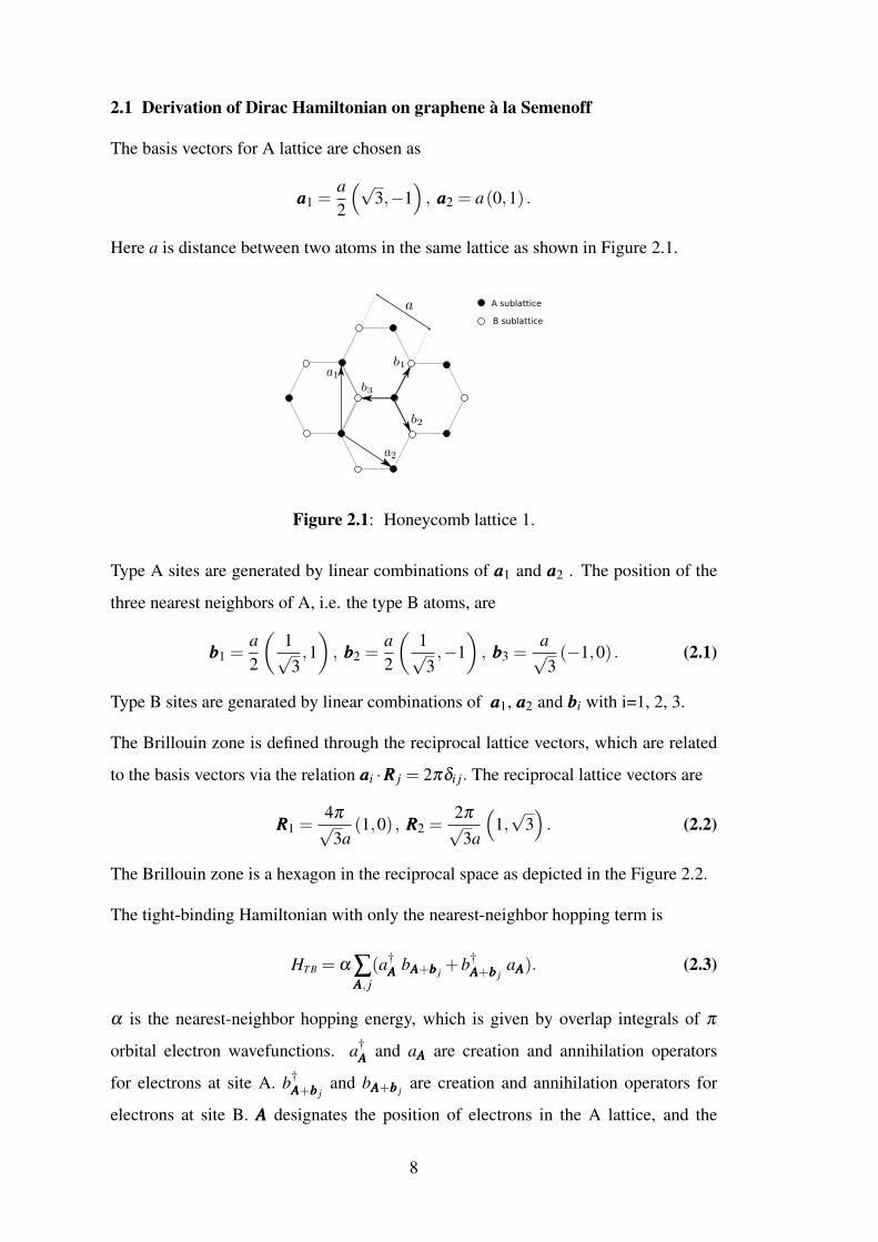
2.1 Derivation of Dirac Hamiltonian on graphene à la Semenoff

The basis vectors for A lattice are chosen as

aaa1 =a2

(√3,−1

), aaa2 = a(0,1) .

Here a is distance between two atoms in the same lattice as shown in Figure 2.1.

A sublattice

B sublattice

Figure 2.1: Honeycomb lattice 1.

Type A sites are generated by linear combinations of aaa1 and aaa2 . The position of the

three nearest neighbors of A, i.e. the type B atoms, are

bbb1 =a2

(1√3,1), bbb2 =

a2

(1√3,−1

), bbb3 =

a√3(−1,0) . (2.1)

Type B sites are genarated by linear combinations of aaa1, aaa2 and bbbi with i=1, 2, 3.

The Brillouin zone is defined through the reciprocal lattice vectors, which are related

to the basis vectors via the relation aaai ·RRR j = 2πδi j. The reciprocal lattice vectors are

RRR1 =4π√3a

(1,0) , RRR2 =2π√3a

(1,√

3). (2.2)

The Brillouin zone is a hexagon in the reciprocal space as depicted in the Figure 2.2.

The tight-binding Hamiltonian with only the nearest-neighbor hopping term is

HT B = α ∑AAA, j

(a†AAA bAAA+bbb j +b†

AAA+bbb jaAAA). (2.3)

α is the nearest-neighbor hopping energy, which is given by overlap integrals of π

orbital electron wavefunctions. a†AAA and aAAA are creation and annihilation operators

for electrons at site A. b†AAA+bbb j

and bAAA+bbb j are creation and annihilation operators for

electrons at site B. AAA designates the position of electrons in the A lattice, and the

8

Figure 2.2: Brillouin zone 1 and degeneracy points.

position of electrons in the B lattice are given by AAA+bbb j. The Fourier transformations

of these operators are

a†AAA =

∫BZ

d2k(2π)2 e−ikkk·AAAa†

kkk, b†AAA+bbb j

=∫

BZ

d2k(2π)2 e−ikkk·(AAA+bbb j)b†

kkk. (2.4)

Using these Fourier transformations, the tight-binding Hamiltonian in k-space

becomes

HT B = α

∫BZ

d2k(2π)2

(a†

kkk b†kkk

)( 0 α ∑ j eikkk·bbb j

α ∑ j e−ikkk·bbb j 0

)(akkkbkkk

). (2.5)

The energy eigenvalues are obtained as

E(k) =±α2∣∣∣ei~k·~b1 + ei~k·~b2 + ei~k·~b3

∣∣∣ . (2.6)

The negative energy states corresponds to states in the valence band and the positive

energy states correspond to states in the conduction band. Degenarcy points

correspond to the roots of (2.6) where the conduction and valence bands meet. There

are two inequivalent degenarcy points, named most commonly as K and K′ points.

The degenarcy points of graphene occur at corners of the Brillouin zone. These two

inequivalent points can be chosen following [5] as

KKK =2π√3a

(1,

1√3

), KKK′ =−KKK. (2.7)

In Figure 2.2, the Brillouin zone and the degeneracy points are shown.

The continuum limit is where a, the distance between two atoms in the same lattice,

goes to zero. In this limit, only states around the degeneracy points contribute to

the dynamics. Hence, in the continuum limit, one is interested in the off-diagonal

9

componens of the Hamiltonian density for the K and K′ valleys:

lima→0

ei(kkk+KKK)·bbb j =

√3a2

(ik1− k2)ei π

3 , lima→0

e−i(kkk+KKK)·bbb j =

√3a2

(−ik1− k2)e−i π

3 ,

lima→0

ei(kkk−KKK)·bbb j =

√3a2

(ik1 + k2)e−i π

3 , lima→0

e−i(kkk−KKK)·bbb j =

√3a2

(−ik1 + k2)ei π

3 .

For the K valley, (2.5) becomes

HK1 = α

√3a2

∫ d2k(2π)2

(a†

kkk−KKK b†kkk−KKK

)( 0 (−ik1− k2)ei 2π

3

(ik1− k2)e−i 2π

3 0

)(akkk−KKKbkkk−KKK

)= α

√3a2

∫ d2k(2π)2

(a†

kkk−KKK b†kkk−KKK

)ei π

3 σ3

(0 −ik1− k2

ik1− k2 0

)e−i π

3 σ3

(akkk−KKKbkkk−KKK

)≡ α

√3a2

d2k(2π)2 Ψ1(−iσ1k1− iσ2k2)Ψ1. (2.8)

Thus, the Dirac Hamiltonian density for the K valley is

HK = vFγµkµ , (2.9)

with the following definition of the spinor and its Dirac conjugate:

Ψ1 =

√√3aα

2e−i σ3π

3

(akkk−KKKbkkk−KKK

), Ψ1 =

√√3aα

2

(a†

kkk−KKK b†kkk−KKK

)ei σ3π

3 γ0. (2.10)

The gamma matrices are chosen as γµ = (σ3, iσ1, iσ2), with µ = 0,1,2. They satisfy

the Clifford algebra with the anti-commutation relation γµ ,γν= 2gµν . The metric is

Minkowski with signature (+,−,−). Here kµ =(0,−kkk), since in this derivation on-site

interaction which would give rise to a mass is not included in the initial tight-binding

Hamiltonian. vF is the effective velocity with which electrons on graphene travel and

is given in terms of α and a as vF = α

√3a2 . For the K′ valley, (2.5) becomes

HK′2 = α

√3a2

∫ d2k(2π)2

(a†

kkk+KKK b†kkk+KKK

)( 0 (−ik1 + k2)e−i 2π

3

(ik1 + k2)ei 2π

3 0

)(akkk+KKKbkkk+KKK

)= α

√3a2

∫ d2k(2π)2

(a†

kkk−KKK b†kkk−KKK

)e−i π

3 σ3

(0 −ik1− k2

ik1− k2 0

)ei π

3 σ3

(akkk−KKKbkkk−KKK

)It is observed that σ1e−i π

3 σ3σ1 = ei π

3 σ3 .

HK′2 = α

√3a2

∫ d2k(2π)2

(a†

kkk−KKK b†kkk−KKK

)σ1ei π

3 σ3

(0 ik1 + k2

−ik1 + k2 0

)e−i π

3 σ3σ1

(akkk−KKKbkkk−KKK

)≡ α

√3a2

∫ d2k(2π)2 Ψ2(iσ1k1 + iσ2k2)Ψ2

Thus, the Dirac Hamiltonian density for the K′ valley is

HK′ =−vFγµkµ , (2.11)

10

with the following definition of the spinor and its Dirac conjugate:

Ψ2 =

√√3aα

2e−i σ3π

3 σ1

(akkk−KKK′

bkkk−KKK′

), Ψ2 =

√√3aα

2

(a†

kkk−KKK′ b†kkk−KKK′

)σ1ei σ3π

3 γ0.

Hence, the Dirac-like Hamiltonian on graphene in the continuum limit takes the form

H =∫ d2k

(2π)2 [Ψ1HKΨ1 + Ψ2HK′

Ψ2]. (2.12)

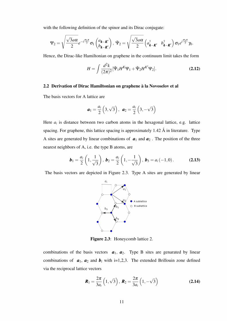
2.2 Derivation of Dirac Hamiltonian on graphene à la Novoselov et al

The basis vectors for A lattice are

aaa1 =al

2

(3,√

3), aaa2 =

al

2

(3,−√

3)

Here al is distance between two carbon atoms in the hexagonal lattice, e.g. lattice

spacing. For graphene, this lattice spacing is approximately 1.42 Å in literature. Type

A sites are generated by linear combinations of aaa1 and aaa2 . The position of the three

nearest neighbors of A, i.e. the type B atoms, are

bbb1 =al

2

(1,

1√3

), bbb2 =

al

2

(1,− 1√

3

), bbb3 = al (−1,0) . (2.13)

The basis vectors are depicted in Figure 2.3. Type A sites are generated by linear

A sublattice

B sublattice

Figure 2.3: Honeycomb lattice 2.

combinations of the basis vectors aaa1, aaa2. Type B sites are genarated by linear

combinations of aaa1, aaa2 and bbbi with i=1,2,3. The extended Brillouin zone defined

via the reciprocal lattice vectors

RRR1 =2π

3al

(1,√

3), RRR2 =

2π

3al

(1,−√

3)

(2.14)

11

is a hexagon. The extended Brillouin zone is a rhombus. The degeneracy points reside

at the corners of the hexagonal Brillouin zone, and can be chosen following [4] as

KKK =2π√3al

(1,

1√3

), KKK′′′ =

2π√3al

(1,− 1√

3

). (2.15)

The Brillouin zone and the degeneracy points are depicted in Figure 2.4.

Figure 2.4: Brillouin zone 2 and degeneracy points.

The tight-binding Hamiltonian with the only the nearest-neighbor hopping term is

HT B =−α ∑AAA, j

(a†AAA bAAA+bbb j +b†

AAA+bbb jaAAA). (2.16)

α is the nearest-neighbor hopping energy. The k-space Hamiltonian is obtained

through the Fourier transformations (2.4).

HT B =−α

∫BZ

d2k(2π)2

(a†

kkk b†kkk

)( 0 α ∑ j eikkk·bbb j

α ∑ j e−ikkk·bbb j 0

)(akkkbkkk

). (2.17)

The off-diagonal componens of the Hamiltonian density for the K and K′ valleys in the

continuum limit yield

limal→0

ei(kkk−KKK)·bbb j =3al

2(k1− ik2)ei π

6 , limal→0

e−i(kkk−KKK)·bbb j =3al

2(k1 + ik2)e−i π

6 ,

limal→0

ei(kkk−KKK′′′)·bbb j =3al

2(k1 + ik2)ei π

6 , limal→0

e−i(kkk−KKK′′′)·bbb j =3al

2(k1− ik2)e−i π

6 .

For the K valley, (2.17) becomes

HK1 =

3alα

2

∫ d2k(2π)2

(a†

kkk−KKK b†kkk−KKK

)ei π

12 σ3

(0 k1− ik2

k1 + ik2 0

)e−i π

12 σ3

(akkk−KKKbkkk−KKK

),

≡ 3alα

2

∫ d2k(2π)2 Ψ

†kkk−KKK(σ1k1 +σ2k2)Ψkkk−KKK.

Then, the Dirac-like Hamiltonian density for the K valley is

Hkkk−KKK = vF(σ1k1 +σ2k2) (2.18)

12

with vF = 3alα2 and the spinor

Ψkkk−KKK = e−i π

12 σ3

(akkk−KKKbkkk−KKK

).

For the K′ valley, (2.17) becomes

HK′2 =

3alα

2

∫ d2k(2π)2

(a†

kkk−KKK′ b†kkk−KKK′

)e−i π

12 σ3

(0 k1 + ik2

k1− ik2 0

)ei π

12 σ3

(akkk−KKK′

bkkk−KKK′

),

≡ 3alα

2

∫ d2k(2π)2 Ψ

†kkk−KKK′(σ1k1−σ2k2)Ψkkk−KKK′.

Then, the Dirac-like Hamiltonian density for the K′ valley is

Hkkk−KKK′ = vF(σ1k1−σ2k2) (2.19)

with vF = 3alα2 and the spinor

Ψkkk−KKK′ = ei π

12 σ3

(akkk−KKK′

bkkk−KKK′

).

vF is the Fermi velocity which is estimated to be on the order 106m/s. The interesting

feature about this Fermi velocity is that it is a constant like the velocity of light, it

does not depend on momentum or energy. It is given in terms of the lattice spacing

and the nearest-neighbor hopping parameter. As a result, the effective Hamiltonian on

graphene takes the form

H =∫ d2k

(2π)2 [Ψ†kkk−KKKHkkk−KKKΨkkk−KKK +Ψ

†kkk−KKK′Hkkk−KKK′Ψkkk−KKK′]. (2.20)

2.3 Derivation of Dirac Hamiltonian on graphene à la Gusynin et al

The basis vectors for A lattice are chosen as [7]

aaa1 =a2

(1,√

3), aaa2 =

a2

(1,−√

3).

Here a is distance between two carbon atoms in the same lattice. It is√

3 times the

lattice spacing, al. Type A sites are generated by linear combinations of aaa1 and aaa2 .

The position of the three nearest neighbors of A, i.e. the type B atoms, are

bbb1 = a(

0,1√3

), bbb2 =−

a2

(−1,

1√3

), bbb3 =−

a2

(1,

1√3

). (2.21)

Type B sites are genarated by linear combinations of aaa1, aaa2 and bbbi with i=1, 2, 3. The

basis vectors are depicted in the Figure 2.5.

13

A sublattice

B sublattice

Figure 2.5: Honeycomb lattice 3.

The extended Brillouin zone defined via the reciprocal lattice vectors

RRR1 =2π

a

(1,

1√3

), RRR2 =

2π

a

(1,− 1√

3

)(2.22)

is a rhombus. The Brillouin zone is a hexagon.

The degeneracy points reside at the corners of the hexagonal Brillouin zone, and can

be chosen following [7] as

KKK =4π

3a(1,0) , KKK′′′ =−4π

3a(1,0) . (2.23)

The Brillouin zone and the choice of degeneracy points are depicted in the Figure 2.6.

The tight-binding Hamiltonian in momentum space is

Figure 2.6: Brillouin zone 3 and degeneracy points.

HT B =−t∫

BZ

d2k(2π)2

(a†

kkk b†kkk

)( 0 ∑ j eikkk·bbb j

∑ j e−ikkk·bbb j 0

)(akkkbkkk

). (2.24)

where the nearest-neigbor hopping parameter t comes with a minus sign. The

off-diagonal componens of the Hamiltonian density for the K and K′ valleys yield

14

in the continuum limit

lima→0

ei(kkk+KKK)·bbb j =a√

32

(−k1 + ik2), lima→0

e−i(kkk+KKK)·bbb j =a√

32

(−k1− ik2),

lima→0

ei(kkk+KKK′′′)·bbb j =a√

32

(k1 + ik2), lima→0

e−i(kkk+KKK′′′)·bbb j =a√

32

(k1− ik2).

For the K valley, (2.24) becomes

Hk+K =at√

32

∫ d2k(2π)2

(a†

kkk+KKK b†kkk+KKK

)( 0 k1− ik2k1 + ik2 0

)(akkk+KKKbkkk+KKK

),

≡ at√

32

∫ d2k(2π)2 Ψ

†kkk+KKK(σ1k1 +σ2k2)Ψkkk+KKK.

Then, the Dirac-like Hamiltonian density for the K valley is

Hkkk+KKK = vF(σ1k1 +σ2k2) (2.25)

with vF = at√

32 and the spinor

Ψkkk+KKK =

(akkk+KKKbkkk+KKK

).

For the K′ valley, (2.24) becomes

Hk+K′ =at√

32

∫ d2k(2π)2

(a†

kkk+KKK′ b†kkk+KKK′

)( 0 −k1− ik2−k1 + ik2 0

)(akkk+KKK′

bkkk−KKK′

),

≡ at√

32

∫ d2k(2π)2 Ψ

†kkk+KKK′(−σ1k1 +σ2k2)Ψkkk+KKK′.

Then, the Dirac-like Hamiltonian density for the K′ valley is

Hkkk+KKK′ = vF(−σ1k1 +σ2k2), (2.26)

with vF = at√

32 and the spinor

Ψkkk+KKK′ =

(akkk+KKK′

bkkk+KKK′

).

As a result, the effective Hamiltonian on graphene takes the form

H =∫ d2k

(2π)2 [Ψ†kkk+KKKHkkk+KKKΨkkk+KKK +Ψ

†kkk+KKK′Hkkk+KKK′Ψkkk+KKK′]. (2.27)

Investigating the Hamiltonian densities (2.25) and (2.26), one can observe that they

can elegantly be treated in one Hamiltonian density in the form

HG = vF(σ1⊗ τ3k1 +σ2⊗111τk2), (2.28)

15

incorporating all degrees of freedom discussed in this section. The Pauli matrices σi

describe the two sublattices A and B and τ3 = diag(1,−1) describes the K and K′

valleys. Then, the corresponding Hamiltonian is

H ≡∫ d2k

(2π)2 Ψ†GHGΨG, (2.29)

with four-component spinors Ψ†G =

(a†

kkk+KKK b†kkk+KKK a†

kkk+KKK′ b†kkk+KKK′

).

There are numerous articles on graphene, where the derivation of the Dirac-like

Hamiltonian is presented. In this section, three of the most prominent ones were

presented. The point is that the choice of unit cell basis vectors determines the position

of Dirac points in the k-space and therefore affects the representation of Dirac matrices.

Semenoff’s derivation was originally done to comment on the parity anomaly in 2+1

quantum field theory, therefore it is relativistic. The derivation of Novoselov et al was

discussed in this section to present another perspective and because of the fact that the

discussion of electronic properties of graphene usually is based on this derivation. The

result of the derivation of Gusynin et al enables one to smoothly relate to Kane-Mele

model on graphene, which will be broadly investigated in the rest of the thesis.

2.4 Foldy-Wouthuysen transformation and Berry gauge fields

In this section, the Foldy-Wouthuysen transformation of the Dirac Hamiltonian and

Berry gauge field in terms of Foldy-Wouthuysen transformation will be presented.

Relativistic electrons of charge e > 0 with a characteristic velocity like the velocity

of light c or the effective velocity vF as in graphene will be considered. To retain the

formulation general, h= c= vF = 1, as well as e= 1. The constants will be recuperated

when needed. The free, massive electrons are described by the Dirac Hamiltonian

H = ααα · kkk+βm. (2.30)

In this section vectors are d-dimensional, like the momentum kkk whose components are

denoted kI; I = 1, · · · ,d. The Hamiltonian (2.30) can be diagonalized as

UHU† = Eβ , (2.31)

where E is the total energy

E =√

k2 +m2, (2.32)

16

and U is the unitary Foldy-Wouthuysen transformation

U =βH +E√2E(E +m)

.

Through the transformation U a pure gauge field can be introduced as

A U = iU(kkk)∂U†(kkk)

∂kkk. (2.33)

Pure gauge field is a gauge field whose curvature vanishes. The Berry gauge field

A is obtained by projecting (2.33) onto the positive energy eigenstates of the Dirac

Hamiltonian (2.30). One can be convinced that eliminating the negative energy states

is equivalent to the adiabatic approximation by revoking its similarity to suppression

of the interband interactions in molecular problems [42]. Thus, we define the Berry

gauge field as

AAA≡ PA UP, (2.34)

where P is the projection operator onto the positive energy subspace. This definition of

the Berry gauge field is valid irrespective of the dimensions of the Hamiltonian (2.30).

In order to derive AAA explicitly let us adopt the following 2N×2N ; N = [d2 ], dimensional

realizations of ααα and β

ααα =

(0 ρρρ

ρρρ† 0

), β =

(1 00 −1

). (2.35)

Here ρρρ and the unit matrix 1 are 2N−1×2N−1 dimensional. In the representation (2.35)

the gauge field (2.33) becomes

A UI =

i2E2(E +m)

[E(E +m)αIβ +βααα · kkkkI− iEσIJkJ] , (2.36)

where σIJ ≡− i2 [αI,αJ]. Therefore, the Berry gauge field (2.34) results to be

AI =−i

4E(E +m)(ρIρ

†J −ρJρ

†I )kJ. (2.37)

Although the field strength of (2.36) vanishes because of being a pure gauge field, the

Berry curvature

GIJ =∂AJ

∂kI− ∂AI

∂kJ− i[AI,AJ], (2.38)

is non-vanishing in general.

When in 2n+1 dimensional space-time where n = 1,2 · · · , the Berry curvature (2.38)

can be employed to define the Chern number which is the integrated Chern character,

as [43]

Nn =1

(4π)nn!

∫M2n

d2nk εI1I2···I2ntr

GI1I2 · · ·GI2n−1I2n

. (2.39)

17

For 2 + 1 dimensional systems the Berry gauge field is Abelian, so that Gab =

∂Ab/∂ka−∂Aa/∂kb, where a,b = 1,2, and the first Chern number is

N1 =1

4π

∫d2kεabtrGab. (2.40)

In 4+1 dimensions one introduces the second Chern number as

N2 =1

32π2

∫d4kεi jkltrGi jGkl, (2.41)

where i, j,k, l = 1,2,3,4.

18

3. RELATION BETWEEN THE SPIN HALL CONDUCTIVITY AND THESPIN CHERN NUMBER FOR DIRAC-LIKE SYSTEMS

In ferromagnets, in response to the electric field a spontaneous Hall current can be

generated. A semiclassical formulation of this anomalous Hall effect was given in [16]

within the Fermi liquid theory. There, the anomalous Hall conductivity was calculated

considering the equations of motion in the presence of the Berry gauge fields derived

from the Bloch wave function. When this system is subjected to an external magnetic

field, the definition of the particle density and the electric current should be made

appropriately. Nevertheless, the computed value of the anomalous Hall conductivity

remains unaltered [17,44,45]. Hall currents without a magnetic field can be generated

also in fermionic systems described by Dirac-like Hamiltonians [9]. Taking into

account the spin of electrons, these systems yield Hall currents due to the spin transport

which is known as the spin Hall effect [8] or Chern insulator. We would like to

present a semiclassical formulation of the spin Hall conductivity using a differential

form formalism for fermions which are described by Dirac-like Hamiltonians.

In semiclassical kinetic theory, the spin degrees of freedom can be considered by

treating them as dynamical variables. However to calculate the spin Hall conductivities

it would be more appropriate to keep the Hamiltonian and the related Berry gauge

fields as matrices in “spin indices". In this respect a differential form formalism

was presented in [24]. Dynamical variables in this semiclasical formalism are the

usual space coordinates and momenta but the symplectic form is matrix valued. We

will show that this formalism is suitable to calculate the spin Hall conductivity for

Dirac-like systems. We deal with electrons, so that without loss of generality we

consider the third component of spin denoted by Sz, whose explicit form depends on

the details of the underlying Dirac-like Hamiltonian. When the third component of

spin is conserved at the quantum level, constructing the spin current is straightforward.

However, spin Hall effect can persist even if the third component of spin is not

conserved. In the latter case semiclassical definition of the spin Hall conductivity is not

very clear. Within the Kane-Mele model of graphene (2+ 1 dimensional topological

19

insulator) [8] it was argued that one cannot anymore use the Berry curvature to obtain

the main contribution to the spin Hall effect when the spin nonconserving Rashba

term is present [46]. We will show that even for the systems where the spin is not

a good quantum number, it is always possible to establish the leading contribution

to the spin Hall effect in terms of the Berry field strength derived in the appropriate

basis. Moreover, we will demonstrate that it is always given in terms of the spin Chern

number which is defined to be one half the difference of the Chern numbers of spin-up

and spin-down sectors [20]. A similar claim was made in [47] by employing the Green

function within the Kubo formalism.

The formulation will be illustrated within the Kane-Mele model of graphene:

When only the intrinsic spin-orbit coupling is present, the third component of the

spin is a good quantum number and the spin Hall conductivity can be acquired

straightforwardly in terms of the Berry curvature [34]. When the Rashba term is

switched on, the third component of spin ceases to be conserved. Nevertheless, we will

show that by choosing the correct basis one can still establish the leading contribution

to the spin Hall conductivity by the Berry curvature. It is given by the spin Chern

number calculated in [48].

The starting point of the method is the matrix valued symplectic form [15, 24]. We

will show that it can be obtained in terms of the wave packets formed by the positive

energy solutions of Dirac-like equations adapting the formalism of [21, 22]. The

formalism of deriving the velocities of phase space variables in terms of the phase

space variables themselves will be presented in Section 3.2. It leads to the anomalous

Hall effect straightforwardly as we will discuss briefly in Section 3.3. Definition of

the spin current is presented in Section 3.4. It is shown that if one adopts the correct

definition of the spin current in two space dimensions the essential part of the spin Hall

conductivity is always given by the spin Chern number. We will illustrate the method

by applying it to the Kane-Mele model first in the absence and then in the presence of

Rashba coupling.

20

3.1 Wave-packet dynamics

Dirac equation possesses negative and positive energy solutions. Obviously one

can form a wave packet by superposing only positive energy solutions. However,

relativistic invariance of the Dirac theory demands to superpose both positive and

negative solutions. Nevertheless by ignoring the relativistic momenta one can deal

with only a wave packet composed of positive energy solutions. Indeed this is the

starting point of the semiclassical approximation. We denote the spinor corresponding

to a positive energy solution of Dirac equation by u(α)(ppp,xxxc), which is a function of

the momentum ppp, and the position of the wave packet center in coordinate space xxxc :

H0(ppp)u(α)(ppp,xxxc) = Eαu(α)(ppp,xxxc); Eα > 0.

The normalization is

u†(α)(ppp,xc)u(β )(ppp,xc) = δαβ . (3.1)

Let us consider the following wave packet obtained by superposing only positive

energy solutions labeled by the superscript α ,

Ψxxx ≡Ψxxx(pppc,xxxc) =∫[d p]|a(ppp, t)|e−iγ(ppp,t)

∑α

ξαψ(α)xxx (ppp,xxxc), (3.2)

where [d p] denotes the measure of the d dimensional momentum space. The

distribution |a(ppp, t)|e−iγ(ppp,t) has a peak at the wave packet center pppc and satisfies∫|a|2[d p] = 1. The expansion coefficients ξα are also normalized, ∑α |ξα |2 = 1.

ψ(α)xxx (ppp,xxxc) is composed of two parts

ψ(α)xxx (ppp,xxxc) = u(α)(ppp,xxxc)φxxx(ppp), (3.3)

with

φxxx(ppp) =1

(2π)d/2 e−ippp·xxx.

The normalization is ∫[d p]φ?

xxx (ppp)φyyy(ppp) = δ (xxx− yyy).

When the position operator, xxx acts on φxxx(ppp) we get

xxxφxxx(ppp) = i∂

∂ pppφxxx(ppp) = xxxφxxx(ppp).

21

and the completeness relation is∫[dx]φ?

xxx (ppp)φxxx(qqq) = δ (ppp− qqq). As a result of these

definitions, (3.3) has the following normalization∫[dx]ψ†(α)

xxx (ppp,xxxc)ψ(β )xxx (qqq,xxxc) = δαβ δ (ppp−qqq). (3.4)

We would like to calculate the expectation value of the position operator over the wave

packet (3.2). The calculation proceeds as follows; we first calculate xΨxxx, in which we

use

xxxψ(α)xxx = u(α)(ppp,xxxc)xxxφxxx(ppp) = u(α)(ppp,xxxc)xxxφxxx(ppp) = u(α)(ppp,xxxc)(i

∂

∂ ppp)φxxx(ppp).

Integrating by parts, we obtain

xxxΨxxx = −i∫[d p]

∂ |a(ppp, t)|∂ ppp

e−iγ(ppp,t)∑α

ξαu(α)(ppp,xxxc)φxxx(ppp)

−∫[d p]|a(ppp, t)|∂γ(ppp, t)

∂ pppe−iγ(ppp,t)

∑α

ξαu(α)(ppp,xxxc)φxxx(ppp)

− i∫[d p]|a(ppp, t)|e−iγ(ppp,t)

∑α

ξα

∂u(α)(ppp,xxxc)

∂ pppφxxx(ppp).

Then we reach the following result∫[dx]Ψ†

xxxxΨxxx = −i∫[d p]|a(ppp, t)|∂ |a(ppp, t)|

∂ ppp(3.5)

−∫[d p]|a(ppp, t)|2 ∂γ(ppp, t)

∂ ppp− i∫[d p]|a(ppp, t)|2 ∑

α,β

ξ∗β

u†(β )(ppp,xxxc)∂u(α)(ppp,xxxc)

∂ pppξα .

The first term vanishes since∫|a|2[d p] = 1. The second and the third terms are

obtained using (3.4). The distribution has the mean momentum, pppc defined through

pppc =∫[d p]ppp|a(ppp, t)|2.

Thus, for any function f (ppp), we get

f (pppc) =∫[d p] f (ppp)|a(ppp, t)|2. (3.6)

Using the definition (3.6) in (3.5), and observing that the expectation value of the

position operator over the wave packet (3.2) is xxxc, which is the center of the wave

packet in coordinate space, xxxc =∫[dx]Ψ†

xxxxΨxxx, we obtain

xxxccc =−∂γc

∂ pppc− i ∑

α,β

ξ∗β

u†(β )(pppc,xxxc)∂

∂ pppcu(α)(pppc,xxxc)ξα . (3.7)

22

We define γc ≡ γ(pppc, t). We would like to define the one-form η through dS ,

dS =∫[dx]Ψ†

xxx (id−H0dt)Ψxxx = dγc +∑αβ

ξ∗αη

αβξβ .

We start by computing

dΨxxx = dt∂Ψxxx

∂ t+dxxxc

∂Ψxxx

∂xxxc

= dt∫[d p]

∂

∂ t|a(ppp, t)|e−iγ(ppp,t)

∑α

ξαu(α)(ppp,xxxc)φxxx(ppp)

− idt∫[d p]|a(ppp, t)|∂γ(ppp, t)

∂ te−iγ(ppp,t)

∑α

ξαu(α)(ppp,xxxc)φxxx(ppp)

+ dxxxc

∫[d p]|a(ppp, t)|e−iγ(ppp,t)

∑α

ξα

∂

∂xxxcu(α)(ppp,xxxc)φxxx(ppp).

So that we obtain∫[dx]Ψ†

xxxidΨxxx = dt∂γc

∂ t+ idxxxc ∑

αβ

ξ∗β

u†(β )(pppc,xxxc)∂

∂xxxcu(α)(pppc,xxxc)ξα .

To transform the first term, we use dγc = dt ∂γc∂ t +d pppc

∂γc∂ pppc

and (3.7). Then∫[dx]Ψ†

xxxidΨxxx = dγc+d pppc ·xxxc+id pppc ∑αβ

ξ∗β

u†(β ) ∂

∂ pppcu(α)

ξα +idxxxc ∑αβ

ξ∗β

u†(β ) ∂

∂xxxcu(α)

ξα

This is a convenient point to define the following matrix valued Berry gauge fields

iu†(α)(pppc,xxxc)∂

∂xxxcu(β )(pppc,xxxc) = aaaαβ , (3.8)

iu†(α)(pppc,xxxc)∂

∂ pppcu(β )(pppc,xxxc) = AAAαβ . (3.9)

The Dirac-like free Hamiltonian only depends on the derivatives with respect to xxx, so

that we get ∫[dx]Ψ†

xxxH0(∂

∂xxx)Ψxxx = ∑

αβ

ξ∗αEα(pppc)δ

αβξβ .

Thus, by defining Hαβ

0 = Eαδ αβ , we obtain

dS =∫[dx]Ψ†

xxx (id−H0dt)Ψxxx = dγc+∑αβ

ξ∗α

(d pppc ·xxxcδ

αβ +dxxxcaaaαβ +d pppcAAAαβ−Hαβ

0 dt)

ξβ .

Then we can define the matrix valued one-form ηαβ as,

ηαβ = δ

αβ xxxc ·d pppc +aaaαβ ·dxxxc +AAAαβ ·d pppc−Hαβ

0 dt, (3.10)

which governs dynamics of the wave-packet.

Before moving onto the semiclassical formalism stemming from the matrix valued

23

one-form, ηαβ . Here, an alternative derivation will be presented. The derivation starts

from the following wave-packet

Ψxxx ≡ Ψxxx(pppc,xxxc, t) = ∑α

ξα(pppc, t)u(α)(pppc,xxxc)e−ipppc·xxx, (3.11)

The normalization of u(α)(pppc,xxxc) is given by (3.1). The one-form η is defined through

dS ,

dS =∫[dx]δ (xxx− xxxc)Ψ

†xxx (id−H0dt)Ψxxx = i∑

α

ξ∗αdξα +∑

αβ

ξ∗αη

αβξβ .

The exact derivative of (3.11) yields

dΨxxx = dt∂ Ψxxx

∂ t+dxxxc

∂ Ψxxx

∂xxxc+d pppc

∂ Ψxxx

∂ pppc

= dt ∑α

∂ξα

∂ tu(α)e−ipppc·xxx +dxxxc ∑

α

ξα

∂u(α)

∂xxxce−ipppc·xxx +d pppc ∑

α

∂ξα

∂ pppcu(α)e−ipppc·xxx

+ d pppc ∑α

ξα

∂u(α)

∂ pppce−ipppc·xxx +d pppc ∑

α

ξαu(α)(−ixxx)e−ipppc·xxx.

Thus,∫[dx]δ (xxx− xxxc)Ψ

†xxxidΨxxx = idt ∑

α

ξ∗α

∂ξα

∂ t+ idxxxc ∑

αβ

ξ∗αu†(α)∂u(β )

∂xxxcξβ +d pppcxxxc

+ id pppc ∑α

ξ∗α

∂ξα

∂ pppc+ id pppc ∑

αβ

ξ∗αu†(α)∂u(β )

∂ pppcξβ

Using the definitions of Berry gauge fields given in (3.8), (3.9), and defining Hαβ

0 =

Eαδ αβ , the following expression is obtained

dS = i∑α

ξ∗αdξα +∑

αβ

ξ∗α

(δ

αβ id +d pppc · xxxcδαβ +dxxxcaaaαβ +d pppcAAAαβ −Hαβ

0 dt)

ξβ .

Ignoring the time dependence, (3.10) is obtained straightforwardly.

3.2 Semiclassical formalism

In the previous section, the semiclassical theory established in terms of the wave

packet composed of positive energy solutions is presented. It yields a semiclassical

description of the system whose dynamics is governed by gauge fields which are

matrices labeled by “spin indices". It is so called because the basis of the wave packets

are solutions of a Dirac-like Hamiltonian. Obviously range of this index depends on

the spacetime dimension as well as on the intrinsic properties of the system considered.

24

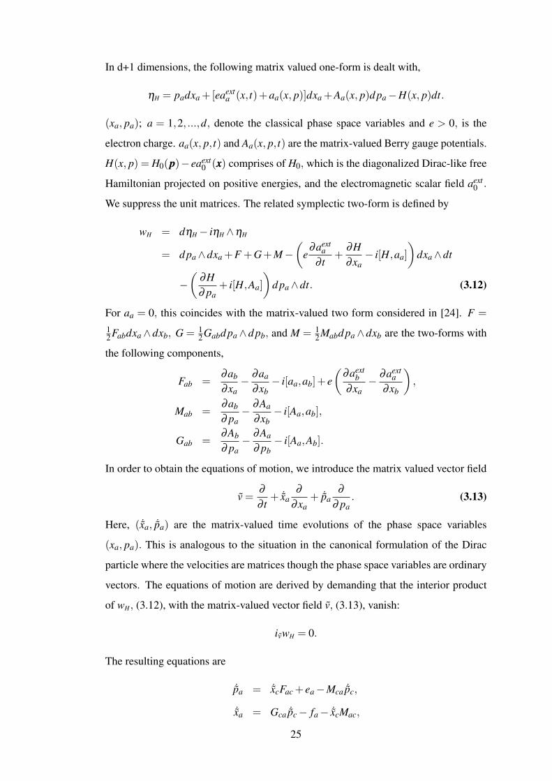
In d+1 dimensions, the following matrix valued one-form is dealt with,

ηH = padxa +[eaexta (x, t)+aa(x, p)]dxa +Aa(x, p)d pa−H(x, p)dt.

(xa, pa); a = 1,2, ...,d, denote the classical phase space variables and e > 0, is the

electron charge. aa(x, p, t) and Aa(x, p, t) are the matrix-valued Berry gauge potentials.

H(x, p) = H0(ppp)−eaext0 (xxx) comprises of H0, which is the diagonalized Dirac-like free

Hamiltonian projected on positive energies, and the electromagnetic scalar field aext0 .

We suppress the unit matrices. The related symplectic two-form is defined by

wH = dηH− iηH ∧ηH

= d pa∧dxa +F +G+M−(

e∂aext

a∂ t

+∂H∂xa− i[H,aa]

)dxa∧dt

−(

∂H∂ pa

+ i[H,Aa]

)d pa∧dt. (3.12)

For aa = 0, this coincides with the matrix-valued two form considered in [24]. F =

12Fabdxa∧dxb, G = 1

2Gabd pa∧d pb, and M = 12Mabd pa∧dxb are the two-forms with

the following components,

Fab =∂ab

∂xa− ∂aa

∂xb− i[aa,ab]+ e

(∂aext

b∂xa

− ∂aexta

∂xb

),

Mab =∂ab

∂ pa− ∂Aa

∂xb− i[Aa,ab],

Gab =∂Ab

∂ pa− ∂Aa

∂ pb− i[Aa,Ab].

In order to obtain the equations of motion, we introduce the matrix valued vector field

v =∂

∂ t+ ˙xa

∂

∂xa+ ˙pa

∂

∂ pa. (3.13)

Here, ( ˙xa, ˙pa) are the matrix-valued time evolutions of the phase space variables

(xa, pa). This is analogous to the situation in the canonical formulation of the Dirac

particle where the velocities are matrices though the phase space variables are ordinary

vectors. The equations of motion are derived by demanding that the interior product

of wH, (3.12), with the matrix-valued vector field v, (3.13), vanish:

ivwH = 0.

The resulting equations are

˙pa = ˙xcFac + ea−Mca ˙pc,

˙xa = Gca ˙pc− fa− ˙xcMac,

25

where we defined

ea ≡ eEa + i[H0,aa],

fa ≡ −∂H0

∂ pa+ i[H0,Aa],

in terms of the external electric field Ea = ∂aext0 /∂xa−∂aext

a /∂ t.

The Lie derivative of the volume form Ωd+1 = (−1)[d2 ]

d! wdH ∧ dt can be used to attain

the matrix-valued velocities ( ˙xa, ˙pa) in terms of the phase space variables (xa, pa). It

will be illustrated for d = 2, due to the fact that basically we are interested in 2+ 1

spacetime dimensional Dirac-like systems. In 2+ 1 dimensions, where the extended

phase space is 5 dimensional, the volume form reads

Ω2+1 =−12

wH ∧wH ∧dt. (3.14)

We express it through the canonical volume element of the phase space dV , as

Ω2+1 = w1/2dV ∧dt, (3.15)

where w1/2 is the Pfaffian of the following 4×4 matrix,(Fi j −δi j−Mi j

δi j +Mi j −Gi j

).

We do not treat the spin indices on the same footing with the phase space indices

(xi, pi); i = 1,2. Thus the Pfaffian w1/2 is a matrix in spin indices. The Lie derivative

associated with the vector field (3.13) of the volume form (3.15) can be expressed

formally as

LvΩ2+1 =(ivd+div)(w1/2dV ∧dt)=(

∂

∂ tw1/2 +

∂

∂xi( ˙xiw1/2)+

∂

∂ pi(w1/2 ˙pi)

)dV ∧dt.

(3.16)

Actually, to obtain it explicitly one should employ the definition (3.14) yielding

LvΩ2+1 =−12

dw2H.

Comparing the exterior derivative of

wH ∧wH = d pi∧dxi∧d p j∧dx j +2M∧d pi∧dxi +2eidxi∧dt ∧d p j∧dx j

+ (F fi + fiF)∧d pi∧dt +(Mei + eiM)∧dxi∧dt

+ 2 fid pi∧dt ∧d p j∧dx j +F ∧G+G∧F +(M fi + fiM)∧d pi∧dt

+ (Gei + eiG)∧dxi∧dt,

26

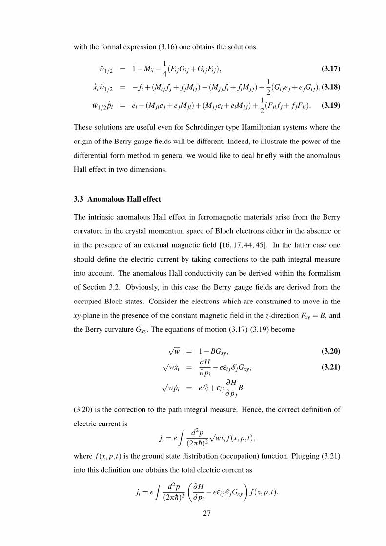
with the formal expression (3.16) one obtains the solutions

w1/2 = 1−Mii−14(Fi jGi j +Gi jFi j), (3.17)

˙xiw1/2 = − fi +(Mi j f j + f jMi j)− (M j j fi + fiM j j)−12(Gi je j + e jGi j), (3.18)

w1/2 ˙pi = ei− (M jie j + e jM ji)+(M j jei + eiM j j)+12(Fji f j + f jFji). (3.19)

These solutions are useful even for Schrödinger type Hamiltonian systems where the

origin of the Berry gauge fields will be different. Indeed, to illustrate the power of the

differential form method in general we would like to deal briefly with the anomalous

Hall effect in two dimensions.

3.3 Anomalous Hall effect

The intrinsic anomalous Hall effect in ferromagnetic materials arise from the Berry

curvature in the crystal momentum space of Bloch electrons either in the absence or

in the presence of an external magnetic field [16, 17, 44, 45]. In the latter case one

should define the electric current by taking corrections to the path integral measure

into account. The anomalous Hall conductivity can be derived within the formalism

of Section 3.2. Obviously, in this case the Berry gauge fields are derived from the

occupied Bloch states. Consider the electrons which are constrained to move in the

xy-plane in the presence of the constant magnetic field in the z-direction Fxy = B, and

the Berry curvature Gxy. The equations of motion (3.17)-(3.19) become

√w = 1−BGxy, (3.20)

√wxi =

∂H∂ pi− eεi jE jGxy, (3.21)

√wpi = eEi + εi j

∂H∂ p j

B.

(3.20) is the correction to the path integral measure. Hence, the correct definition of

electric current is

ji = e∫ d2 p

(2π h)2

√wxi f (x, p, t),

where f (x, p, t) is the ground state distribution (occupation) function. Plugging (3.21)

into this definition one obtains the total electric current as

ji = e∫ d2 p

(2π h)2

(∂H∂ pi− eεi jE jGxy

)f (x, p, t).

27

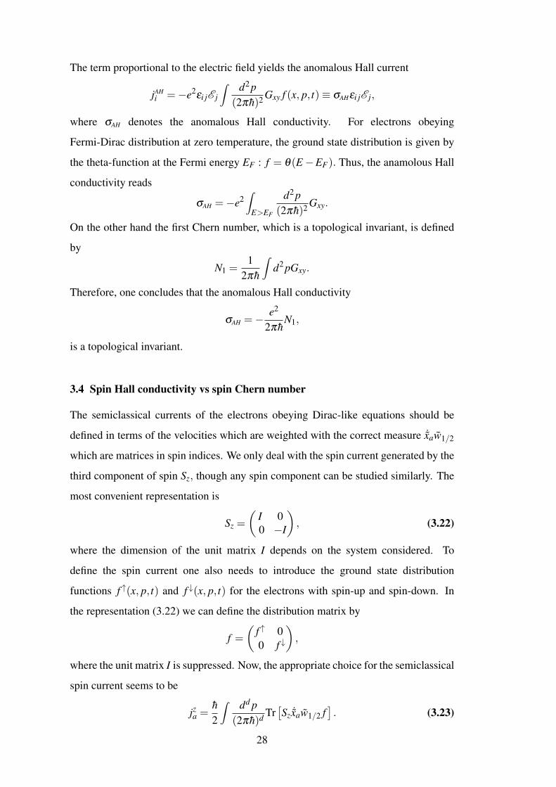
The term proportional to the electric field yields the anomalous Hall current

jAHi =−e2

εi jE j

∫ d2 p(2π h)2 Gxy f (x, p, t)≡ σAHεi jE j,

where σAH denotes the anomalous Hall conductivity. For electrons obeying

Fermi-Dirac distribution at zero temperature, the ground state distribution is given by

the theta-function at the Fermi energy EF : f = θ(E−EF). Thus, the anamolous Hall

conductivity reads

σAH =−e2∫

E>EF

d2 p(2π h)2 Gxy.

On the other hand the first Chern number, which is a topological invariant, is defined

by

N1 =1

2π h

∫d2 pGxy.

Therefore, one concludes that the anomalous Hall conductivity

σAH =− e2

2π hN1,

is a topological invariant.

3.4 Spin Hall conductivity vs spin Chern number

The semiclassical currents of the electrons obeying Dirac-like equations should be

defined in terms of the velocities which are weighted with the correct measure ˙xaw1/2

which are matrices in spin indices. We only deal with the spin current generated by the

third component of spin Sz, though any spin component can be studied similarly. The

most convenient representation is

Sz =

(I 00 −I

), (3.22)

where the dimension of the unit matrix I depends on the system considered. To

define the spin current one also needs to introduce the ground state distribution

functions f ↑(x, p, t) and f ↓(x, p, t) for the electrons with spin-up and spin-down. In

the representation (3.22) we can define the distribution matrix by

f =(

f ↑ 00 f ↓

),

where the unit matrix I is suppressed. Now, the appropriate choice for the semiclassical

spin current seems to be

jza =

h2

∫ dd p(2π h)d Tr

[Sz ˙xaw1/2 f

]. (3.23)

28

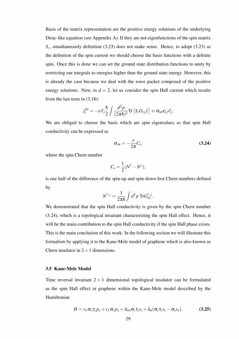
Basis of the matrix representation are the positive energy solutions of the underlying

Dirac-like equation (see Appendix A). If they are not eigenfunctions of the spin matrix

Sz, simultaneously definition (3.23) does not make sense. Hence, to adopt (3.23) as

the definition of the spin current we should choose the basis functions with a definite

spin. Once this is done we can set the ground state distribution functions to unity by

restricting our integrals to energies higher than the ground state energy. However, this

is already the case because we deal with the wave packet composed of the positive

energy solutions. Now, in d = 2, let us consider the spin Hall current which results

from the last term in (3.18):

jSHi =−eE j

h2

∫ d2 p(2π h)2 Tr

[SzGi j f

]≡ σSHεi jE j.

We are obliged to choose the basis which are spin eigenvalues so that spin Hall

conductivity can be expressed as

σSH =− e2π

Cs, (3.24)

where the spin Chern number

Cs =12(N↑−N↓),

is one half of the difference of the spin-up and spin-down first Chern numbers defined

by

N↑,↓ =1

2π h

∫d2 p TrG↑,↓xy .

We demonstrated that the spin Hall conductivity is given by the spin Chern number

(3.24), which is a topological invariant characterizing the spin Hall effect. Hence, it

will be the main contribution to the spin Hall conductivity if the spin Hall phase exists.

This is the main conclusion of this work. In the following section we will illustrate this

formalism by applying it to the Kane-Mele model of graphene which is also known as

Chern insulator in 2+1 dimensions.

3.5 Kane-Mele Model

Time reversal invariant 2 + 1 dimensional topological insulator can be formulated

as the spin Hall effect in graphene within the Kane-Mele model described by the

Hamiltonian

H = vFσxτz px + vFσy py +∆SOσzτzsz +λR(σxτzsy−σysx). (3.25)

29

It is the effective theory of electrons on graphene with the Fermi velocity vF .

The intrinsic and Rashba spin-orbit coupling constants are denoted by ∆SO and λR,

respectively. σx,y,z are the Pauli matrices in the representation σz = diag(1,−1), which

act on the states of sublattices. τz = diag(1,−1), labels the states at the Dirac points

(valleys) K and K′, and the Pauli matrices, sx,y,z act on the real spin space in the

representation where the third component is diagonal sz = diag(1,−1).

The main difference between the Kane-Mele model with and without the Rashba

spin-orbit coupling term lies in whether the third component of spin is a good quantum

number or not. In the former case sz is conserved and application of the semiclassical

approach is straightforward. However, also in the latter case the spin Hall conductivity

is non-vanishing with the condition ∆SO > λR. We will illustrate how the semiclassical

formulation can be applied in both cases and demonstrate that main contribution to the

spin Hall conductivity is always given by the spin Chern number defined in [20].

3.6 Kane-Mele model without the Rashba spin-orbit interaction term

In this case the Hamiltonian is

HSO = vFσxτz px + vFσy py +∆SOσzτzsz. (3.26)

In fact, there are four different two dimensional Hamiltonians stemming from (3.26):

HSO =

H↑+ 0 0 0

0 H↑− 0 00 0 H↓+ 00 0 0 H↓−

.

These two dimensional Hamiltonians corresponding to the ↑, ↓ spin and the K, K′

valley are

H↑+ = vF(σx px +σy py)+∆SOσz, H↑− = vF(−σx px +σy py)−∆SOσz, (3.27)

H↓+ = vF(σx px +σy py)−∆SOσz, H↓− = vF(−σx px +σy py)+∆SOσz. (3.28)

The effect of the spin-orbit term is to create a gap in the energy band structure of the

Hamiltonians. In terms of the eigenvalues of the momenta hkkk, (3.27) and (3.28) yield

the same energy distribution

E =±√

v2F h2k2 +∆2

SO, (3.29)

30

corresponding to particle and antiparticle (hole) states.

Note that in this section ppp is not a quantum operator but denotes the classical phase

space variable.

We deal with four different two dimensional Dirac-like theories (3.27), (3.28), thus

we should take into account the contributions arising from each of them separately.

We adopt the formulation of [42] to derive the Berry gauge fields arising from

each one of the two dimensional Hamiltonians (3.27), (3.28). Therefore, we should

start with giving the unitary Foldy-Wouthuysen transformations (U↑+,U↑−,U↓+,U↓−)

corresponding to the Dirac-like Hamiltonians (H↑+,H↑−,H↓+,H↓−). We would like

to present them in the unified notation:

U ≡ diag(U↑+,U↑−,U↓+,U↓−).

The unitary Foldy-Wouthuysen transformation U can be engaged to define the gauge

field [42, 50]

A ≡ diag(A ↑+,A ↑−,A ↓+,A ↓−) = ihU(ppp)∂U†(ppp)

∂ ppp.

Exploring the Dirac-like Hamiltonians (3.27), (3.28), we introduce the following

Foldy-Wouthuysen transformation

U =1√

2E(E +∆SO)

σzH↑++E 0 0 0

0 −σzH↑−+E 0 00 0 −σzH↓++E 00 0 0 σzH↓−+E

,

(3.30)

where E is the positive energy depending on ppp as E =√

v2F ppp2 +∆2

SO. Observe that

(3.30) is defined to satisfy

HSO =UHU† = Eσzτzsz. (3.31)

One can study each entry of (3.30) as in [42] and show that they lead to the gauge

potential

A U =ih

2E2(E +∆SO)

[vFE(E +∆SO)ααασzτzsz + v3

Fσzτzsz(ααα · ppp)ppp+ v2FE(ααα · ppp)ααα− v2

F pppE].

Its components can be written explicitly as [34]

A Ux =

h(vFE(E +∆SO)σysz− v3F(σy px−σxτz py)sz px + v2

FEσzτz py)

2E2(E +∆SO), (3.32)

A Uy =

h(−vFE(E +∆SO)σxτzsz− v3F(σy px−σxτz py)sz py− v2

FEσzτz px)

2E2(E +∆SO).(3.33)

31

Because of being a pure gauge potential the field strength of A U vanishes. However,

one can consider the adiabatic approximation by projecting on the positive energy

states:

AAA≡ PA UP. (3.34)

By inspecting the positive eigenvalues of the (3.31) one can deduce that the projection

operator P is

P≡ diag(P↑+,P↑−,P

↓+,P

↓−) = diag(1,0,0,1,0,1,1,0).

It should be noted that when projected on positive energy states only the last terms in

(3.32) and (3.33) make nonvanishing contributions, so that the Abelian Berry gauge

field is

Ai =hv2

F

2E(E +∆SO)εi j p j111τsz, (3.35)

where the unit matrix 111τ in the τz space is exhibited explicitly. It is worth emphasizing

that in A negative energy states are present, thus it possesses twice the matrix elements

of A B. The nonvanishing component of the Berry curvature is given as

G = h(

∂Ay

∂ px− ∂Ax

∂ py

)≡ diag(G↑+,G

↑−,G

↓+,G

↓−) =−

h2v2F∆SO

2E3 111τsz. (3.36)

The spin Hall effect in graphene can be given as [19] as

σSH =−e2

∫ E(2)F d2 p

(2π h)2

[(G↑++G↑−)− (G↓++G↓−)

]. (3.37)

E(2)F denotes the highest energy level occupied in the two dimensional system. Thus,

inserting (3.36) into the definition (3.37) leads to

σSH = −e2

∫ E(2)F

−∞

d2 p(2π h)2

(−2h2v2

F∆SO

E3

)= − e

2π

∆SO

E(2)F

. (3.38)

This in accord with the calculation of the spin Hall conductivity obtained by employing

the Kubo formula which is presented in Appendix B.

We let the Fermi energy level of graphene lie in the gap, so that in (3.38) we set

E(2)F = ∆SO and obtain the spin Hall conductivity as

σSH =− e2π

.

32

This is the value established in [8]. Based on the above derivation of spin Hall

conductivity, in the rest of the section the semiclassical treatment presented before

will be employed. U can be employed to acquire the eigenfunctions of (3.26) as

u(α)(p) =U†v(α),

where v(1) = (1,0 · · · ,0)T , · · · ,v(8) = (0,0 · · · ,1)T . The Hamiltonian projected on

positive energy eigenstates in the presence of the external electric field E is

HSO0 = (E + eE · xxx)111τ111s.

In the rest of this section we will keep the unit matrices explicit. The Berry gauge field

is given by (3.35). Hence, the corresponding Berry curvature is given by (3.36). In the

absence of a magnetic field the phase space measure (3.17) is trivial: w1/2 = 1. Thus,

the equations of motion (3.18)-(3.19) yield

˙xi = −v2F pi

Eτzsz− eεi jE jGxy,

˙pi = eEi111τ111s.

In the representation which we adopted the third component of spin becomes

Sz = 111τsz. (3.39)

Note that u(α) are also the eigenstates of the spin matrix (3.39). Therefore, the

distribution matrix f = 111τdiag( f ↑, f ↓) is adequate to define the spin current by

jzi =

h2

∫ d2 p(2π h)2 Tr

[Sz√

w ˙xi f].

It yields the spin Hall current jSHi = σSHεi jE j, where the spin Hall conductivity is given

by

σSH =−eh2

∫ d2 p(2π h)2 Tr [SzGxy] . (3.40)

Let us decompose (3.40) such that the contributions arising from spin subspace and K,

K′ valleys become apparent. One can easily observe that

σSH = −eh2

∫ d2 p(2π h)2 (G

↑Kxy −G↓Kxy +G↑K

′xy −G↓K

′xy )

= − e4π

(N↑K1 −N↓K1 +N↑K′

1 −N↓K′

1 ).

Each contribution is associated with the first Chern number of the related subspace.

This has been observed in [34] where the related Chern numbers were calculated. We

33

conclude that the spin Hall conductivity is proportional to the sum of the spin Chern

number of the K valley, CKs and the spin Chern number of the K′ valley, CK′

s :

σSH =− e2π

(CKs +CK′

s ) =− e2π

Cs =−e

2π.

In the absence of Rashba term we defined the spin current straightforwardly since the

Hamiltonian (3.26) commutes with sz.

3.7 Kane-Mele model with Rashba spin-orbit interaction term

Although, in the presence of the Rashba term sz does not commute with the

Hamiltonian (3.25), the spin Hall effect still exists for ∆SO > λR [8, 49, 51]. However,

the semiclassical calculation is not clear as we discussed in Section 3.4. There we also

discussed the correct definition of spin current. Nevertheless, before proceeding as

indicated in Section 3.4 let us carry on with the computation of the Berry gauge field

naively using the positive energy eigenfunctions of (3.25).

The K and K′ subspaces corresponding to τz = ±1 yield the same energy eigenvalues

and eigenstates which are presented in Appendix B. Thus, it is sufficient to consider

only the 4×4 Hamiltonian in K subspace denoted by HK :

HKΦα = EαΦα ,

where α = 1, ..,4 and the energy eigenvalues Eα are

E1 = λ +

√(∆SO−λ )2 + v2

F p2, E2 =−λ +

√(∆SO +λ )2 + v2

F p2,

E3 = λ −√(∆SO−λ )2 + v2

F p2, E4 =−λ −√

(∆SO +λ )2 + v2F p2. (3.41)

We deal with the coupling constants satisfing ∆SO > 2λR, so that E1,E2 and E3,E4 are

positive and negative, respectively.

The diagonalized Hamiltonian is H ΦK = diag(E1,E2,E3,E4). When we project on the

positive energy eigenstates and take both of the contributions coming from the K and

K′ subspaces, the Hamiltonian becomes

HΦ0 = 111τ

(E1 00 E2

)+ eE · xxx111τ111s.

The Berry gauge field turns out to be Abelian:

AΦi = hεi j

p j

p2 111τ

(−1 2N1N2

2N1N2 −1

).

34

The corresponding Berry curvature GΦxy = (∂xAφ

y −∂yAφx ), can easily be computed as

GΦxy = 111τ

(0 −2h

p ∂p(N1N2)

−2hp ∂p(N1N2) 0

).

According to (3.17)-(3.19) the equations of motion calculated in the energy

eigenfunction basis are

˙xi = −111τv2F pi

(1

E1−λ0

0 1E2+λ

)+2

N1N2

p2 εi j p j(E1−E2)111τsy− eεi jE j111τGΦxy,

˙pi = eEi111τ111s,

where we set w1/2 = 1.

The spin current cannot be defined by (3.23) with a diagonal f . Choosing it diagonal

would lead to a vanishing spin Hall current due to the fact that

Tr[SzGΦ

xy]= 0.

The difficulty stems from the fact that energy eigenfunctions are not simultaneously

eigenstates of the spin operator Sz = diag(sz,sz). In K subspace eigenstates of the spin

operator Sz, constructed from the energy eigenstates Φα , are

Ψ1 =1√2(Φ1 +Φ2), Ψ2 =

1√2(Φ1−Φ2),

Ψ3 =1√2(Φ3 +Φ4), Ψ4 =

1√2(Φ3−Φ4).

Ψ1,Ψ2 and Ψ3,Ψ4 correspond to positive and negative energy sectors, respectively.

They satisfy

SzΨ1,3 = Ψ1,3, SzΨ2,4 =−Ψ2,4.

The Hamiltonian in Ψα basis is obtained by the transformation

H ΨK =UΨHKU†

Ψ,

where U†Ψ

=(Ψ1 Ψ2 Ψ3 Ψ4

). Notice that UΨ is related to the unitary

transformation that diagonalizes HK, denoted by UΦ, via UΨ = RUΦ, where R =(R 00 R

)with

R =1√2

(1 11 −1

).

35

Thus we acquired

H Ψ = (111τR)H Φ(R111τ)

=12

E1 +E2 E1−E2 0 0E1−E2 E1 +E2 0 0

0 0 E3 +E4 E3−E40 0 E3−E4 E3 +E4

111τ .

The Hamiltonian in Ψα basis projected on positive energy eigenstates in the presence

of external electric field E , is

HΨ0 = (E1 +E2)111τ111s +(E1−E2)111τsx + eE · xxx111τ111s.

The basis transformation R sustains the connection between AAAΨ and AAAΦ via the relation

AAAΨ = (111τ R)AAAΦ(R111τ), so that

AΨi = hεi j

p j

p2 111τ

(−1+2N1N2 0

0 −1+2N1N2

)≡ 111τ

(A↑i 00 A↓i

).

The corresponding Berry curvature GΨxy = (111τ R)GΦ

xy(R111τ) is calculated as

GΨxy =−

2hp

∂ (N1N2)

∂ p111τsz ≡ 111τ

(G↑xy 0

0 G↓xy

).

Hence, the equations of motion are

˙xi = −111τv2F pi

(1

E1−λ+ 1

E2+λ

1E1−λ

− 1E2+λ

1E1−λ

− 1E2+λ

1E1−λ

+ 1E2+λ

)−2

N1N2

p2 εi j p j(E1−E2)111τsy− eεi jE jGΨxy,

˙pi = eEi111τ111s.

The spin Hall current can now be written as

jSHi =−eh

2εi jE j

∫ d2 p(2π h)2 Tr

[SzGΨ

xy f],

where f = 111τdiag( f ↑, f ↓). Therefore, f restricts the integral to positive energies and

the spin Hall conductivity becomes

σSH =−eh2

∫ d2 p(2π h)2

(GK↑

xy −GK↓xy )+(GK′↑

xy −GK′↓xy )=− e

2π(CK

s +CK′s ) =− e

2πCs.

In [48] this spin Chern number is calculated as Cs = 1. Therefore, we conclude that

σSH =− e2π

.

Indeed, in [8] it was argued that the value of the spin Hall conductivity sligtly differs

from this value which is confirmed either in terms of numerical methods [49] or

deriving the related effective theory [51].

36

4. EFFECTIVE FIELD THEORY OF TIME-REVERSAL INVARIANTTOPOLOGICAL INSULATORS

The 2+ 1 dimensional topological field theory of the integer quantum Hall effect is

considered in Section 4.1 in order to recall how to construct the TRI spin quantum

Hall effect in graphene which is a model of 2+ 1 dimensional topological insulator.

Then, the dimensional reduction to 1+1 dimensions by obtaining the one dimensional

charge polarization explicitly is presented. In Section 4.2, the 4 + 1 dimensional

Chern-Simons field theory which was shown to describe the fundamental topological

insulator is considered. The field strengths of the related Berry gauge fields are derived

to obtain the second Chern number and dimensional reduction to 3+ 1 dimensions is

studied. By imitating the approach of [8] a hypothetical model is theorized in 4+ 1

dimensions which yields a TRI spin Hall current in 3+ 1 dimensions by means of

the dimensional reduction. Slightly modifying the approach of [37], a dimensional

reduction procedure to 2+1 dimensions is proposed which provides explicit forms of

the gauge field components which take part in the descendant action.

4.1 2+1 Dimensional topological insulator and dimensional reduction to 1+1

dimension

Field theory of electrons interacting with the external Abelian gauge field Aα is given

by the Dirac Lagrangian density

L (ψ, ψ,A) = ψ [γα (pα +Aα)−m]ψ, (4.1)

where α = 0,1 · · ·d. By integrating out the fermionic degrees of freedom in the related

path integral one formally gets the action of the external fields as

S[A] =−i lndet[iγα(∂α − iAα)−m]. (4.2)

For d = 2n one of the terms which it gives rise to is [38]

T [An+1] =∫[dq1] · · · [dqn+1]Aα1(q1) · · ·Aαn+1(qn+1)πα1···αn+1(q1 · · ·qn+1).

37

[dq] denotes the integral over the related phase space. At the order of first loop

πα1···αn+1(q1 · · ·qn+1)=∫ d2n+1k

(2π)2n+1 trG(k)λα1(k,k−q1)G(k−q1) · · ·λαn+1(k+qn+1,k),

where G(k) is the one particle Green function of the free Dirac field and λα is the

photon vertex. T [An+1] generates the 2n+1 dimensional Chern-Simons term

S2n+1e f f [A] =Cn

∫d2n+1xε

α1···α2n+1Aα1∂α2Aα3 · · ·∂α2nAα2n+1, (4.3)

which can be taken as the effective topological action in the low energy limit.

In 2 + 1 dimensions integration of the massive Dirac fermions in the related path

integral with the Lagrangian density (4.1) leads to the effective topological action

S2+1e f f [A] =C1

∫d3xε

µνρAµ∂νAρ , (4.4)

where µ,ν ,ρ = 0,1,2.

On the other hand, plugging the field strength (2.38) of the Abelian Berry gauge field

(2.34) into (2.40) leads to

N1 =i

2π

∫d2kεabtrP∂aU∂bU†P.

Therefore, we conclude that

C1 =N1

4π. (4.5)

One can observe that by employing (4.5) in (4.4) the effective topological action of

external gauge fields coupled to massive Dirac electrons living in 2+ 1 dimensions

becomes

S2+1e f f =

N1

4π

∫d3xε

µνρAµ∂νAρ . (4.6)

To calculate the related first Chern number (2.40), let us choose the representation

ααα = (σx,σy), where σa are the Pauli spin matrices. This corresponds to set ρa = (1,−i)

in (2.37). Thus, the Abelian Berry gauge field can be written as

Aa =εabkb

2E(E +m). (4.7)

It yields the Berry curvature

F12 =

(∂A2

∂k1− ∂A1

∂k2

)=− m

2E3 . (4.8)

38

We plug (4.8) into (2.40) and perform the change of variable by (3.41) to express the

related first Chern number as

N1 =−m2

∫D

dEE2 , (4.9)

where the domain of integration D will be specified according to the model considered.

If it is required to treat the E > 0 and E < 0 domains on the same footing, we can deal

with

N1 =−m2

∫ m

−∞

dEE2 −

m2

∫∞

−m

dEE2 = 1. (4.10)

4.1.1 A model for 2+1-dimensional topological insulator

Before presenting the graphene model of [8], let us briefly recall the interconnection

between the quantum Hall effect and the Chern-Simons action in 2+ 1 dimensions.

For electrons moving on a surface in the presence of the external in-plane electric field

EEE = (Ex,Ey,0) and the perpendicular magnetic field B = (0,0,Bz) the Hall current is

given by

ja = σHεabEb. (4.11)

Ignoring the spin of electrons the Hall conductivity is a topological invariant [10, 60]:

σH =e2

hN1. (4.12)

Here N1 is the first Chern number resulting from the field strength FB of the Berry

gauge field obtained from the single particle Bloch wave functions which are solutions

of the Schrödinger equation in the presence of the external magnetic field Bz,

integrated over the states up to the Fermi level EF as

N1 =∫ EF d2k

(2π)2 FB. (4.13)

A field theoretic description is possible in terms of the Chern-Simons action (4.6) with

the definition (4.13). In fact, the current obtained from the topological field theory

(4.6),

jµ =N1

2πεµνρ∂

νAρ ,

gives for Ea = ∂aA0−∂0Aa the Hall current (4.11). It also leads to the charge density

j0 = σHB, where the induced magnetic field is B = ∂xAy− ∂yAx. Note that B would

also be generated by the Hall current (4.11) through the current conservation condition

∂a ja = −∂t j0. We would like to emphasize the fact that the field theory (4.6) is not

39

aware of the external magnetic field Bz. External magnetic field is responsible of

creating the energy spectrum whose consequences are encoded in the calculation of

the first Chern number (4.13).

By employing the Berry gauge field derived from the Dirac equation (4.7), we can

still get the Hall conductivity as in (4.12) by an appropriate choice of the domain of

integration D in (4.9). This construction does not necessitate an external magnetic

field. For the first time in [9] Haldane described how to obtain the quantum Hall

effect without a magnetic field (vanishing in the average) through a Dirac like theory.

To calculate the Hall conductivity following from the Dirac equation we let all the

negative energy levels be occupied up to the Fermi level EF = m in (4.9), so that

σH =e2

h

(−m

2

∫ m

−∞

dEE2

)=

e2

2h. (4.14)

In [8] Kane and Mele incorporated the spin of electrons into the Haldane model [9]

and proposed the following Hamiltonian for graphene

HG = σxτzkx +σyky +mσzτzsz, (4.15)

which leads to a TRI spin current. The mass term is generated by a spin-orbit

coupling. The Pauli spin matrices σx,y,z act on the states of sublattices. The matrix

τz = diag(1,−1) denotes the Dirac points K, K′ which should be interchanged under

the time reversal transformation. The other Pauli matrix sz = diag(1,−1) describes

the third component of the spin of electrons which should also be inverted under time

reversal transformation. Thus the time reversal operator is given by T = UK where

we can take U = τysy and K takes the complex conjugation as well as maps kkk→−kkk.

Therefore (4.15) is TRI:

T HGT−1 = HG.

The Abelian Berry gauge field obtained from the Hamiltonian (4.15) can be written

as [34]

Aa =1

2E(E +m)εabkb1τsz, (4.16)

where 1τ is the unit matrix in the τz space. The corresponding field strength is

F12 ≡ diag(F ↑+,F

↑−,F

↓+,F

↓−) =−

m2E3 1τsz. (4.17)

The indices ↑↓ and ± label, respectively, the third component of the spin and τz. The

spin current defined as

jjjs = jjj↑++ jjj↑−− jjj↓+− jjj↓−,

40

leads to the spin Hall current

jsa = σSHεabEb.

The difference of the related first Chern numbers

∆N1 =1

2π

∫ E=m

E=−∞

d2k[(F ↑

++F ↑−)− (F ↓

++F ↓−)]

= (12+

12)− (−1

2− 1

2) = 2, (4.18)

gives the spin Hall conductivity σSH as

σSH =e

4π∆N1 =

e2π

. (4.19)

4.1.2 Dimensional reduction to 1+1 dimensions

We would like to discuss dimensional reduction from 2+ 1 to 1+ 1 dimensions by

slightly modifying the procedure described in [37]. The dimensionally reduced theory

can be defined through the 1+1 dimensional Lagrangian density

L1+1 (ψ, ψ,A) = ψ [γr (pr +Ar)+ γ2ζy−m]ψ,

where r = t,x and the external field ζy(t,x) is the reminiscent of the gauge field Ay. We

define ζy = ky +ζ , where ky is a parameter which permits us to deal with one particle

Green function of the 2+ 1 dimensional theory to derive the effective action of the

external fields. In fact, integrating out the spinor fields ψ, ψ in the related path integral

yields the effective action

S1+1e f f = G1D(ky)

∫dxdtζ (x, t)εrs∂rAs.

The coefficient G1D(ky) is required to satisfy∫G1D(ky)dky = N1, (4.20)

where the first Chern number N1 is given by (4.9). Instead of the Cartesian coordinates

we prefer to work with the polar coordinates k, θ , where kx = k cosθ , ky = k sinθ .

Similar to (4.20) we would like to introduce G(θ) satisfying∫ 2π

0G(θ)dθ = N1, (4.21)

and define the (1+1)-dimensional effective action as

S1+1 = G(θ)∫

dxdtζ (x, t)εrs∂rAs. (4.22)

41

Although it can be deduced directly from the definition (4.21), we can also obtain G(θ)

by writing the components of the Abelian Berry gauge field (4.16) in polar coordinates:

Aθ =− k2E(E +m)

, Ak = 0.

The Berry curvature remains the same

Fkθ =1k

[∂ (kAθ )

∂k− ∂Ak

∂θ

]=− m

2E3 ,

and allows us to calculate explicitly G(θ) as

G(θ) =1

2π

∫kdkFkθ

= − m4π

∫D

dEE2 =

N1

2π.

Now, one can define the one dimensional charge polarization [52, 53] P(θ) by

∂P(θ)∂θ

≡ G(θ). (4.23)

Adopting the first Chern number calculated in (4.10), N1 = 1, we solve (4.23) by

P(θ) =θ

2π. (4.24)

The physical observable is not directly the charge polarization given by P(θ) but the

adiabatic change in P(θ) along a loop, which is equal to

∆P = P(2π)−P(0) = 1.

The (1+1)-dimensional action (4.22) becomes

S1+1 =1

2π

∫dxdtArεrs∂sζ (x, t), (4.25)

for N1 = 1. The action (4.25) leads to the current

jr =1

2πεrs∂sζ (x, t),

known as the Goldstone-Wilczek formula [54] and gives the charge

Q =1

2π

∫∂ζ (x, t)

∂xdx =

12π

∆ζ .

In fact, it corresponds to solitons on polyacetylene with charge Q= 1/2 for ζ changing

from 0 to π and Q = 1/3 for ∆ζ = 2π/3 as it was obtained in [54].

42

4.2 4+1 Dimensional topological insulator and dimensional reduction to 3+1 and

2+1 dimensions

The topological field theory

S4+1e f f [A] =

N2

24π2

∫d5xε

ABCDEAA∂BAC∂DAE , (4.26)

is designated as the effective action of the 4+1 dimensional TRI topological insulators

in [37]. It follows from (4.3). To derive the related second Chern number N2 we

deal with the 4+ 1 dimensional realization of the Dirac Hamiltonian (2.30) which is

provided by

α1,2,3 =

(0 iσ1,2,3

−iσ1,2,3 0

), α4 =

(0 −1−1 0

), β =

(1 00 −1

). (4.27)

Observing that ρi = (iσ1, iσ2, iσ3,−1), the non-Abelian Berry gauge fields can be

obtained from (2.37) as

A1 =σ3k2−σ2k3−σ1k4

2E(E +m), A2 =

−σ3k1 +σ1k3−σ2k4

2E(E +m), (4.28)

A3 =σ2k1−σ1k2−σ3k4

2E(E +m), A4 =

σ1k1 +σ2k2 +σ3k3

2E(E +m). (4.29)

By definition the Berry gauge field corresponding to the 4 + 1 dimensional Dirac

Hamiltonian can also be derived by considering the explicit solutions of the Dirac

equation as it was done in [55]. They work in the chiral representation, so that the

Berry gauge field components which they obtain differ from (4.28),(4.29).

One can show that the field strength components Fi j = ∂A j/∂ki − ∂Ai/∂k j −

i[Ai,A j], are

F12 =1

2E3(E +m)

[σ3(−E(E +m)+ k2

1 + k22)+σ2(k1k4− k2k3)−σ1(k2k4 + k1k3)

],

F13 =1

2E3(E +m)

[σ2(E(E +m)− k2

1− k23)+σ1(k1k2− k3k4)+σ3(k1k4 + k2k3)

],

F14 =1

2E3(E +m)

[σ1(E(E +m)− k2

1− k24)−σ2(k1k2 + k3k4)−σ3(k1k3− k2k4)

],

F23 =1

2E3(E +m)

[σ1(−E(E +m)+ k2

2 + k23)−σ2(k1k2 + k3k4)−σ3(k1k3− k2k4)

],

F24 =1

2E3(E +m)

[σ2(E(E +m)− k2

2− k24)−σ1(k1k2− k3k4)−σ3(k1k4 + k2k3)

],

F34 =1

2E3(E +m)

[σ3(E(E +m)− k2

3− k24)+σ2(k1k4− k2k3)−σ1(k2k4 + k1k3)

].

43

Plugging them into (2.41) and taking the trace yield

N2 =3

4π2

∫(− m

2E5 )d4k. (4.30)

To calculate it explicitly, we would like to deal with the four dimensional polar

coordinates given by k1 = k cosφ1, k2 = k sinφ1 cosφ2, k3 = k sinφ1 sinφ2 cosφ3 and

k4 = k sinφ1 sinφ2 sinφ3, where the angles φ1,φ2,φ3, respectively, take values in the in-

tervals [0,π], [0,π], [0,2π]. The volume element is d4k = k3 sin2φ1 sinφ2dkdφ1dφ2dφ3.

Hence, after the change of variable by (3.41), one can show that (4.30) can be written

as

N2 =3m4

∫D

m2−E2

E4 dE. (4.31)

When D is taken to be an overlap of the E > 0 and E < 0 domains, we may deal with

N2 =3m4

∫ m

−∞

m2−E2

E4 dE +3m4

∫∞

−m

m2−E2

E4 dE = 1. (4.32)

4.2.1 Dimensional reduction to 3+1 dimensions

Dimensional reduction of the 4+1 dimensional effective action given by (4.1) to 3+1

dimensions can be described by the Lagrangian density

L3+1[ψ, ψ,A] = ψ[γ

α (pα +Aα)+ γ4θ −m]

ψ, (4.33)

where α = 0, · · · ,3. The external field θ(xα) is the reminiscent of the gauge field

A4. ψ, ψ fields can be integrated out through the one particle Green function of 4+1

dimensional theory introducing the parameter k4 by setting θ = k4+θ(xα). By keeping

track of the phase space volume one can obtain the 3+1 dimensional effective action

as

S3+1e f f =

G3D(k4)

4π

∫d4xθε

αβγη∂αAβ ∂γAη , (4.34)

where the coefficient is given through the condition∫G3D(k4)dk4 = N2. (4.35)

We would like to modify this construction by working with the four dimensional polar

coordinates and proposing that the action describing the descendant theory is given by

S3+1 =G3(φ3)

4π

∫d4xθε

αβγη∂αAβ ∂γAη ,

44

whose coefficient, like (4.35), is required to satisfy the condition∫ 2π

0G3(φ3)dφ3 = N2.

Thus, the coefficient G3(φ3) can be obtained as

G3(φ3) =1

32π2

∫εi jkltr(Fi jFkl)k3 sin2

φ1 sinφ2dkdφ1dφ2 =N2

2π, (4.36)

with the definition (4.31) of the second Chern number N2.

Similar to the one-dimensional charge polarization (4.23) one can associate the

coefficient G3(φ3) to P3(φ3) through the relation [37]∫ 2π

0

∂P3(φ3)

∂φ3dφ3 ≡

∫ 2π

0G3(φ3)dφ3 = N2.

Hence the “magnetoelectric polarization" can be obtained as

P3(φ3) =N2

2πφ3. (4.37)

Observe that like the one-dimensional case, for ∆φ3 = 2π it changes by ∆P3 = 1 if

we choose N2 = 1 as it is calculated in (4.32). P3(φ3) depends linearly on φ3 due to

the fact that the second Chern character corresponding to free Dirac particle depends

only on k. Interacting Dirac particles may give rise to polarizations which would not

be linearly dependent on φ3.

By inserting the definition (4.36) into (4.34) the effective action becomes

S3+1 =N2

8π2

∫d4xθε

αβγη∂αAβ ∂γAη . (4.38)

It can be written equivalently as

S3+1 =1

4π

∫d4xP3(θ)ε

αβγη∂αAβ ∂γAη ,

where P3(θ) = N2θ/2π. This describes the axion electrodynamics which is invariant

under the shift θ → θ +2π [3, 56].

45

4.2.2 A hypothetical model for 3+1 dimensional topological insulators

In spite of the fact that the underlying topological gauge theory (4.26) is manifestly

TRI, the theory given by the descendant action (4.38) is TRB except for the values

θ = 0,π. Nevertheless, we may deal with the TRB action (4.38) but introduce a TRI

hypothetical model generalizing the spin Hall effect for graphene [8]. The current

following from the action (4.38) is

jα =N2

(2π)2 εαβγη

∂β θ∂γAη .

Assuming θ = θ(z) and considering the in-plane electric field Ea(x,y); a = 1,2, we

obtain the current [57]

ja =N2

(2π)2 ∂zθ(z)εabEb(x,y). (4.39)

The Hall current can be introduced by integrating (4.39) along the coordinate z as

Ja(x,y)≡∫

jadz = σHεabEb(x,y). (4.40)

It leads to the surface Hall conductivity σH [27, 37]

σH =e2

hN2

(2π)2

∫∂zθdz =

e2

hN2

(2π)2 ∆θ . (4.41)

Obviously we defined ∆θ = θ(∞)− θ(−∞), which is non-vanishing for an adequate

domain wall or at an interface plane between two samples.

Now we should define the second Chern number (4.31) appropriately. We suppose that

all negative energy states are occupied till the Fermi level taken as the first positive

energy value EF = m, so that we get

N2 =3m4

∫ m

−∞

m2−E2

E4 dE = 1/2. (4.42)

Considering a plane of interface which yields ∆θ = 2π the Hall conductivity becomes

σH =e2

2h.

In the representation (4.27) the 4+ 1 dimensional Dirac Hamiltonian (2.30) is TRI

where the time reversal operator can be taken as T4+1 = α2α4K. However, the

Hamiltonian corresponding to the action (4.33) for Aα = 0,

H3+1 = ααα · kkk+α4θ +mβ , (4.43)

46

violates time reversal symmetry. We will present a hypothetical model which is time

reversal invariant emulating the spin Hall effect for graphene. Let αi act on sublattices

with two Dirac points. Assume that around these points which are interchanged under

time reversal transformation, electrons are described by the Hamiltonians as in (4.43).

Moreover the third component of the spin given by the Pauli matrix sz = diag(1,−1)

is included and conserved. Thus, we propose to consider the Hamiltonian

H3+1 = ααα · kkk+ α4θ + τzszβm, (4.44)

where τz = diag(1,−1) and in terms of αi and β given by (4.27) we defined

αi = (α1,τzα2,α3,α4).

Now, as in Section 4.1.1, the time reversal operator interchanging the Dirac points and

the third components of the spin can be defined by T = τysyK, so that (4.44) is TRI.

Obviously, we can obtain (4.44) through the dimensional reduction from the 4 + 1

dimensional action corresponding to the following free Hamiltonian

H = αi · ki + τzszβm≡ diag(H↑+, H↑−, H↓+, H↓−). (4.45)

As we show in Appendix B, the four dimensional Hamiltonians defined by (4.45)

correspond to the second Chern numbers

N↑+2 = N↑−2 =−N↓+2 =−N↓−2 = N2,

where N2 is given by (4.31). Repeating the procedure yielding (4.40)-(4.42) in the

presence of a domain wall we can obtain the dissipationless spin current as

Jsa = J↑+a + J↑−a − J↓+a − J↓−a = σSHεabEb(x,y),

with the spin Hall conductivity

σSH =e

4π

(N↑+2 +N↑−2 −N↓+2 −N↓−2

)=

e2π

.

for ∆θ = 2π . It is equal to the spin Hall conductivity for graphene (4.19).

47

4.2.3 Dimensional reduction to 2+1-dimensions

The 2+1 dimensional Lagrangian density

L2+1[ψ, ψ,A] = ψ[γ

µ(

pµ +Aµ

)+ γ3ζ3 + γ4ζ4−m

]ψ,

describes the dimensionally reduced theory. The fields ζ3(xµ),ζ4(xµ) are the

reminiscent of the gauge fields A3,A4, of the 4+1 dimensionally theory whose action

is given by (4.1) for d = 4. By setting ζ3(xµ) = k3 + φ(xµ) and ζ4(xµ) = k4 + θ(xµ),

where k3,k4 are parameters playing the role of the momentum components in one

particle Green functions. 2+1 dimensional effective action is derived as as

S2+1e f f = G2D(k3,k4)

∫d3xε

µνρAµ∂ν φ∂ρ θ .

Its coefficient should fulfill the condition∫G2D(k3,k4)dk3dk4 = N2. (4.46)

As in Section 4.2.1, we consider the four dimensional polar coordinates and propose

that the action

S2+1 = G2(φ2,φ3)∫

d3xεµνρAµ∂ν φ∂ρ θ , (4.47)

describes the 2+1 dimensional descendant theory. Obviously, like (4.46) we pose the

condition ∫π

0

∫ 2π

0dφ2dφ3G2(φ2,φ3) = N2.

This can be solved by

G2(φ2,φ3) =N2

4πsinφ2.

Proceeding as in [37] we introduce the vector field

Ωµ ≡Ωθ ∂µθ +Ωφ ∂µφ ,

however by adopting the definitions

Ωθ =−N2

4cosφ , Ωφ =−N2

4θ sinφ .

The field strength of the field Ωµ is

∂µΩν −∂νΩµ =N2

2sinφ

(∂νθ∂µφ −∂µθ∂νφ

).

48

Let us define φ = φ2 + φ and θ = φ3 + θ as slowly varying fields, so that at the first

order in derivatives we can write G2(φ ,θ)∂µθ∂νφ ≈ G2(φ2,φ3)∂µ θ ∂ν φ . Therefore,

the action (4.47) can be written in the form

S2+1 =1

2π

∫d3xε

µνρAµ∂νΩρ . (4.48)

The current generated by the field Ωa, a = 1,2, is

jΩa =

e2π

εabEb,

where the electric field is given by Ea = ∂aA0− ∂0Aa. It can be interpreted as the

spin current yielding the spin Hall conductivity σSH = e/2π. Hence, by attributing

the adequate time reversal transformation properties to the gauge field Ωµ , the action

(4.48) corresponds to the TRI 2+ 1 dimensional model of [8] which we discussed in

Section 4.1.1,

The action (4.48) generates the electric current

jµ =1

2πε

µνρ∂νΩρ .

For fields satisfying φ = φ(x), θ = θ(y) it gives the total charge

Q = eN2

4π

∫dxdysinφ∂xφ∂yθ = e

N2

4π

∫π

0sinφdφ

∫ 2π

0dθ = eN2.

On the other hand the three dimensional Skyrmion field nnn coupled to Dirac fermion in

2+1 dimensions yields the current [58]

jTµ =

18π

εµνρnnn ·∂ νnnn×∂ρnnn.

The Skyrmion field configuration discussed in [59] satisfying nnn2 = 1 possesses the

charge QT = 2e. Hence, if we deal with N2 = 1, the Skyrmion theory can be described

for the field configurations satisfying

sinφ(∂νθ∂µφ −∂µθ∂νφ

)=

14

nnn ·∂νnnn×∂µnnn,

which leads to jTµ = 2 jµ . In principle this condition can be solved to obtain nnn in terms

of the fields φ and θ .

Observe also that for the field configurations φ = φ(t), θ = θ(y) the net charge flow

in x direction is ∫dtdy jx =−N2. (4.49)

49

Moreover, we can introduce the magnetoelectric polarization in the form given (4.37)

by defining it as

P3(θ) =−∫

π

0dφΩφ/π =

N2

2πθ .

Then the pumped charge (4.49) can also be written as ∆Q =∫

dP3 = N2 which gives

∆Q = 1/2 for N2 = 1/2, as it is given for the Hall effect (4.42).

50

5. CONCLUSIONS

One of the main topics addressed was the consequences of incorporating spin into the

semiclassical formalism which is described in Section 3. A differential form formalism

was employed. In our semiclassical formalism, acting in the classical phase space

where position and momentum are dynamical variables, but spin comes into play

in the matrix-valuedness of the symplectic 1-form and the Berry gauge fields. This

leads to matrix-valued time evolutions of position and momentum variables. It was

demonstrated that our formalism is suitable to calculate the spin Hall conductivity

for Dirac-like systems. The spin Hall current, thus the spin Hall conductivity was

defined through the time evolutions of position and momentum variables. Dealing with

electrons, without loss of generality the third component of spin was considered whose

explicit matrix form depends on the details of the underlying Dirac-like Hamiltonian.

When the third component of spin is conserved at the quantum level, constructing the

spin current is not intriguing. However, the spin Hall effect can persist even if the

third component of spin is not conserved. Within the Kane-Mele model of graphene, it

was shown in Section 3 that even for the systems where the spin is not a good quantum

number, it is always possible to establish the leading contribution to the spin Hall effect

in terms of the Berry field strength derived in the appropriate basis. Moreover, it was

demonstrated that it is always given in terms of the spin Chern number which is defined

to be one half the difference of the Chern numbers of spin-up and spin-down sectors.

To investigate the Kane-Mele model in 2+ 1 dimensions and topological insulators

in 4+ 1 dimensions, we mainly employ the Foldy-Wouthuysen transformation of the

Dirac Hamiltonian. The Foldy-Wouthuysen transformation diagonalizes the Dirac

Hamiltonian. In order to define the Berry gauge field, the adiabaticity condition

dictates that one should operate within either the positive energy eigenstate states or the

negative energy eigenstates. Thus, the Foldy-Wouthuysen transformation turns out to

be a powerful tool in the investigation of a physical system with topological properties

related to a Dirac-like Hamiltonian. Topological properties are characterized through

the related Chern numbers: The first Chern number in 2+1 dimensions and the second

51

Chern number in 4+1 dimensions acquired by the Berry field strengths.

In Section 4, we deal with the effective field theory of the 4 + 1 dimensional

time-reversal invariant topological insulator. The Foldy-Wouthuysen transformation

was employed to obtain the Berry gauge fields of Dirac Hamiltonian and the first

and second Chern numbers were derived explicitly. In the line of the Kane-Mele

model, a hypothetical model was introduced that yields a dissipationless spin current

in 3 + 1-dimensions. This can be helpful in understanding some aspects of the

three dimensional time-reversal invariant topological insulators if its relation to some

realistic models can be demonstrated. Moreover, in terms of our explicit constructions

one can discuss Z2 topological classification of time-reversal invariant insulators in a

tractable fashion.

In principle our approach can be generalized to the interacting Dirac particles where

the related Foldy-Wouthuysen transformation at least perturbatively exists, where the

inverse of rest energy of the particle is the perturbation parameter. However, it is also

possible to employ h as the perturbation parameter [61]. Recently, the latter approach

attracted considerable interest in the kinetic theory of the chiral particles [62, 63]. We

believe that it suits well in developing our approach to more complicated interacting

Dirac-like systems which can be useful in either condensed matter or high energy

systems.

52

REFERENCES

[1] Jackiw, R. and Rebbi, C. (1976).Solitons with fermion number 12 , Phys. Rev. D,

13(12), 3398–3409.

[2] Su, W. P. , Schrieffer, J. R. and Heeger, A. J. (1979). Solitons in Polyacetylene,Phys. Rev. Lett., 42(25), 1698–1701.

[3] Wilczek, Frank (1987). Two applications of axion electrodynamics, Phys. Rev.Lett., 58(18), 1799–1802.

[4] Castro Neto, A. H., Guinea, F, Peres, N. M. R., Novoselov, K. S. and Geim,A. K. (2009). The electronic properties of graphene, RevModPhys.81.109,81(1), 109–162.

[5] Semenoff, Gordon W. (1984). Condensed-Matter Simulation of aThree-Dimensional Anomaly, Phys. Rev. Lett., 53(26), 2449–2452.

[6] DiVincenzo, D. P. and Mele, E. J. (1984). Self-consistent effective-mass theoryfor intralayer screening in graphite intercalation compounds, Phys. Rev. B,29(4), 1685–1694.

[7] Gusynin, V. P. , Sharapov, S. G. and Carbotte, J. P. (2007). AC Conductivityof graphene:From tight-binding model to 2 + 1-Dimensional quantumelectrodynamics, International Journal of Modern Physics B, 21(27),4611–4658.

[8] Kane, C. L. and Mele, E. J. (2005). Quantum Spin Hall Effect in Graphene, Phys.Rev. Lett., 95(22), 226801.

[9] Haldane, F. D. M. (1988). Model for a Quantum Hall Effect without LandauLevels: Condensed-Matter Realization of the "Parity Anomaly", Phys.Rev. Lett., 61(18), 2015–2018.

[10] Thouless, D. J., Kohmoto, M., Nightingale, M. P.and den Nijs, M. (1982).Quantized Hall Conductance in a Two-Dimensional Periodic Potential,Phys. Rev. Lett., 49(6), 405–408.

[11] Simon, B. (1983). Holonomy,the Quantum Adiabatic Theorem and Berry’s PhasePhys. Rev. Lett., 51(24), 2167–2170.

[12] Kohmoto, M. (1985). Topological Invariant and the Quantization of the HallConductance, Annals of Physics, 160(2), 343 – 354.

[13] Berry, M. V. (1984). Quantal Phase Factors Accompanying Adiabatic Changes,Proc. R. Soc. A, 392(1852), 45–57.

53

[14] Shapere, Aand Wilczek, F (1989) Geometric Phases in Physics (Advanced Seriesin Mathematical Physics), World Scientific.

[15] Dayi, Ö. F. (2008). Spin dynamics with non-Abelian Berry gauge fields as asemiclassical constrained Hamiltonian system , J. Phys. A: Math. Theor.41 (2), 315204.

[16] Haldane, F. D. M. (2004). Berry Curvature on the Fermi Surface: Anomalous HallEffect as a Topological Fermi-Liquid Property, Phys. Rev. Lett., 93(20),206602.

[17] Xiao, Di Shi, Junren and Niu, Qian (2005).Berry Phase Correction to ElectronDensity of States in Solids, Phys. Rev. Lett., 95(13),137204.

[18] Xiao, Di,Chang, M-C. and Niu, Q. (2010). Berry phase effects on electronicproperties, Rev. Mod. Phys., 82(3), 1959–2007.

[19] Chuu, Chih-Piao,Chang, Ming-Che. and Niu, Qian (2009). Semiclassicaldynamics and transport of the Dirac spin, Solid State Communications,150, 533.

[20] Prodan, Emil (2009). Robustness of the spin-Chern number, Phys. Rev. B, 80(12),125327.

[21] Sundaram, Ganesh and Niu, Qian (1999). Wave-packet dynamics in slowlyperturbed crystals: Gradient corrections and Berry-phase effects, Phys.Rev. B, 59(23), 14915.

[22] Culcer, Dimitrie, Yao, Yugui and Niu, Qian (2005). Coherent wave-packetevolution in coupled bands, Phys. Rev. B, 72(8), 085110.

[23] Dayi, Ö. F. and Yunt, E. (2014). Relation between Spin Hall Conductivity andspin Chern Number for Dirac-Like Systems, arXiv: 1408.1596

[24] Dayi, Ö. F. and Elbistan, M. (2014). A Semiclassical Formulation of the ChiralMagnetic Effect and Chiral Anomaly in Even d + 1 Dimensions, arXiv:1402.4727

[25] Hasan, M. Z. and Kane, C. L. (2010). Colloquium, Rev. Mod. Phys., 82(4),3045–3067.

[26] Qi, X-L. and Zhang, S-C. (2011). Topological insulators and superconductors,Rev. Mod. Phys., 83(4), 1057–1110.

[27] Hasan, M. Z. and Moore, Joel E. (2011). Three-Dimensional TopologicalInsulators, Annual Review of Condensed Matter Physics, 2(1), 55–78.

[28] Bernevig, B. A. , Hughes, T. L. and Zhang, S-C. (2006). Quantum Spin HallEffect and Topological Phase Transition in HgTe Quantum Wells, Science,314(5806), 1757–1761.

[29] König, M. , Wiedmann, S. , Wiedmann, S. , Brüne, C., Roth, A., Buhmann, H.,Molenkamp, L.W.,Qi,X-L. and Zhang, S-C. (2007). Quantum Spin HallInsulator State in HgTe Quantum Wells, Science, 318(5851), 766–770.

54

[30] Hasan, M. Z. and Kane, C. L. (2010). Z2 Topological Order and the QuantumSpin Hall Effect, Phys. Rev. Lett., 95(14), 146802.

[31] Niemi, A. J. and Semenoff, G. W. (1983). Axial-Anomaly-Induced FermionFractionization and Effective Gauge-Theory Actions in Odd-DimensionalSpace-Times, Phys. Rev. Lett., 51(23), 2077–2080.

[32] Redlich, A. N. (1984). Gauge Noninvariance and Parity Nonconservation ofThree-Dimensional Fermions, Phys. Rev. Lett., 52(1), 18–21.

[33] Redlich, A. N. (1984). Parity violation and gauge noninvariance of the effectivegauge field action in three dimensions, Phys. Rev. D, 29(10), 2366–2374.

[34] Dayi, Ö. F. and Yunt, E. (2011). Gauge potential formulations of the spin Halleffect in graphene , Physics Letters A, 375(25), 2484.

[35] Zhang, S. C., Hansson, T. H. and Kivelson, S. (1989). Effective-Field-TheoryModel for the Fractional Quantum Hall Effect, Phys. Rev. Lett., 62(1),82–85.

[36] Zhang, S-C. (1992). The Chern-Simons-Landau-Ginzburg Theory of theFractional Quantum Hall Effect Int. J. Mod. Phys. B 6 (01), 25–58.

[37] Qi, X-L. , Hughes, T. L. and Zhang, S-C. (2008). Topological field theory oftime-reversal invariant insulators, Phys. Rev. B, 78(19), 195424.

[38] Dayi, Ö. F., Elbistan, M. and Yunt, E. (2012). Effective field theory of atopological insulator and the Foldy–Wouthuysen transformation, Annalsof Physics, 327(3), 935–951.

[39] Fu, Liang, Kane, C. L. and Mele, E. J. (2007). Topological Insulators in ThreeDimensions, Phys. Rev. Lett., 98(10), 106803.

[40] Moore, J. E. and Balents, L. (2007).Topological invariants oftime-reversal-invariant band structures, Phys. Rev. B, 75(12), 121306.

[41] Roy, Rahul (2009).Topological phases and the quantum spin Hall effect in threedimensions, Phys. Rev. B, 79(19), 195322.

[42] Bérard, A. and Mohrbach, H. (2006). Spin Hall effect and Berry phase ofspinning particles , Physics Letters A, 352(3), 190–195.

[43] Nakahara, M. (1990) Geometry, Topology and Physics, Adam Hilger, Bristol.

[44] Duval, C., Horváth, Z, Horváthy, P. A., Martina, L., and Stichel, P. C..(2006).Comment on “Berry Phase Correction to Electron Density of States inSolids”, Phys. Rev. Lett 96(9), 099701.

[45] Xiao, Di, Shi, Junren and Niu, Qian (2006).Xiao et al. Reply:, Phys. Rev. Lett.,96(9), 099702.

[46] Culcer, Dimitrie, Sinova, Jairo, Sinitsyn, N. A, Jungwirth, T., Mac-Donald, A. H and Niu, Q.. (2004)Semiclassical Spin Transport inSpin-Orbit-Coupled Bands, Phys. Rev. Lett., 93(4), 046602

55

[47] Ezawa, Motohiko (2014).Symmetry protected topological charge in symmetrybroken phase: Spin-Chern, spin-valley-Chern and mirror-Chern numbers,Physics Letters A, 378(16-17), 1180.

[48] Yang, Y., Xu, Z., Sheng, L., Wang, B., Xing, D. Y. and Sheng, D. N. (2011).Time-Reversal-Symmetry-Broken Quantum Spin Hall Effect, Phys. Rev.Lett., 107(6), 066602.

[49] Sheng, L., Sheng, D. N., Ting, C. S.and Haldane, F. D. M. (2005). NondissipativeSpin Hall Effect via Quantized Edge Transport, Phys. Rev. Lett., 95(13),136602.

[50] Murakami, S., Nagaosa, N. and Zhang, S-C. (2003). Dissipationless QuantumSpin Current at Room temperature. Science, 301, 1348.

[51] Dayi, Ö. F. and Elbistan, M.(2013). The effective field theory of (2 +1)-dimensional topological insulator in the presence of Rashba spin–orbitinteraction, J. Phys. A: Math. Theor. 46, 435001.

[52] King-Smith, R. D. and Vanderbilt, David(1993). Theory of polarization ofcrystalline solids, Phys. Rev. B 47(3), 1651.

[53] Ortiz, Gerardo and Martin, Richard M.(1994). Macroscopic polarization as ageometric quantum phase: Many-body formulation, Phys. Rev. B 49(20),14202–14210.

[54] Goldstone, Jeffrey and Wilczek, Frank(1981). Fractional Quantum Numbers onSolitons, Phys. Rev. Lett. 47(14), 986–989.

[55] Ryu, S., Schnyder, A.P., Furusaki, A. and Ludwig, A. W. W. (2010). NewJournal of Physics, 12, 065010.

[56] Vazifeh, M. M. and Franz, M.(2010). Quantization and 2π periodicity of theaxion action in topological insulators, Phys. Rev. B 82(23), 233103.

[57] Boyanovsky, Daniel, Dagotto, Elbio and Fradkin, Eduardo (1987).Anomalouscurrents, induced charge and bound states on a domain wall of asemiconductor, Nuclear Physics B, 285, 340 – 362.

[58] Jaroszewicz, T. (1984). Induced fermion current in the σ model in (2 + 1)dimensions, Physics Letters B, 146(5), 337 – 340.

[59] Grover, T. and Senthil, T. (2008). Topological Spin Hall States, ChargedSkyrmions, and Superconductivity in Two Dimensions, Phys. Rev. Lett.,100(15), 156804.

[60] Avron, J. E., Seiler, R. and Simon, B. (1983). Homotopy and Quantization inCondensed Matter Physics, Phys. Rev. Lett., 51(1), 51–53.

[61] Gosselin, P.,Bérard, A. and Mohrbach, H. (2007). Semiclassical diagonalizationof quantum Hamiltonian and equations of motion with Berry phasecorrections, Eur. Phys. J. B, 58, 137– 148.

56

[62] Manuel, Cristina and Torres-Rincon, Juan M. (2014). Chiral transport equationfrom the quantum Dirac Hamiltonian and the on-shell effective fieldtheory, Phys. Rev. D, 90(7), 076007.

[63] Dwivedi, V. and Stone, M. (2014). Classical chiral kinetic theory and anomaliesin even space-time dimensions, J. Phys. A: Math. Theor. 47 (2), 125401.

57

58

APPENDICES

APPENDIX A: Kubo Formula Derivation of Spin Hall ConductivityAPPENDIX B: Berry Gauge Field and Curvature in 4+1 DimensionsAPPENDIX C: Eigenstates of Kane-Mele Hamiltonian in the Presence of RashbaSpin-orbit Coupling

59

60

APPENDIX A : Kubo Formula Derivation of Spin Hall Conductivity

Introducing the label I =(↑+,↑−,↓+,↓−) corresponding to each of the two dimensionalDirac-like Hamiltonians given in (3.27), (3.28),

|pI〉 and |aI〉 denote, respectively, the positive energy E =√

v2F h2k2 +∆2

SO and thenegative energy −E eigenspinors of the related Dirac-like Hamiltonians. For instance,let us consider the Hamiltonian for the spin up carriers in the K valley, H↑+, whoseeigenspinors can be written in the chiral basis as

|p↑+〉 =

(cos(θ

2 )

sin(θ

2 )eiφ

), (A.1)

|a↑+〉 =

(sin(θ

2 )

−cos(θ

2 )eiφ

), (A.2)

where cosθ = ∆SOE and tanφ =

kykx

. When the Fermi level of graphene is in the gapgenerated by the spin orbit interaction we should set kkk = 0, hence cosθ = 1

we need to consider their eigenspinors. In fact, for the spin up carriers in the K′ valleydescribed with H↑− the eigenspinors are

|p↑−〉 =

(sin(θ

2 )

−cos(θ

2 )e−iφ

), (A.3)

|a↑−〉 =

(cos(θ

2 )

sin(θ

2 )e−iφ

). (A.4)

Similarly, for the spin down carriers in the K valley, we can show that the eigenspinorsof the Hamiltonian H↓+ are

|p↓+〉 =

(sin(θ

2 )

cos(θ

2 )eiφ

), (A.5)

|a↓+〉 =

(cos(θ

2 )

−sin(θ

2 )eiφ

). (A.6)

The eigenspinors of the Hamiltonian H↓− corresponding to the spin down carriers inthe K′ valley are

|p↓−〉 =

(cos(θ

2 )

−sin(θ

2 )e−iφ

), (A.7)

|a↓−〉 =

(sin(θ

2 )

cos(θ

2 )e−iφ

). (A.8)

Kubo formula corresponding to the Hamiltonians (3.27), (3.28) can be written in thenotation introduced as [10]

(σ SH)

I=

eh2

2

∫ E(2)F d2k

(2π)2

2Im[〈aI|y|pI〉〈pI|x|aI〉

]4E2 , (A.9)

61

where x, y are the related velocity operators which can be read from (??) and

E(2)F =

√v2

F h2k2F +∆2

SO.

For H↑+ the velocity operators are x = vFσx, y = vFσy and the eigenspinors |p↑+〉 and|a↑+〉 are given in (A.1) and (A.2). Employing them in (A.9) leads to [?]

(σ SH)↑+ =− e

8π

∆SO

E(2)F

. (A.10)

For the spin up carriers in the K′ valley, we set x =−vFσx, y = vFσy and deal with theeigenspinors (A.3),(A.4). We obtain the same conductivity

(σ SH)↑− =− e

8π

∆SO

E(2)F

. (A.11)

The contributions arising from the spin down carriers in the K and K′ valleys are alsoequal but differ in sign with the spin up contributions:

(σ SH)↓+ = (σ S

H)↓− =

e8π

∆SO

E(2)F

. (A.12)

To obtain the spin Hall conductivity we should take the difference of the spin up andspin down contributions as

σSH = ((σ S

H)↑++(σ S

H)↑−)− ((σ S

H)↓++(σ S

H)↓−). (A.13)

Inserting (A.10), (A.11) and (A.12) into (A.13) leads to the spin Hall conductivity

σSH =− e

2π

∆SO

E(2)F

.

This is the same with the result obtained in terms of the Berry phase (3.38).

62

APPENDIX B : Berry Gauge Field and Curvature in 4+1 Dimensions

The Hamiltonian (4.45) which comprises τz and spin degrees of freedom denoted ±and ↑↓, respectively, yields the 4+1 dimensional Dirac Hamiltonians

H↑+ = α1k1 +α2k2 +α3k3 +α4k4 +mβ , H↑− = α1k1−α2k2 +α3k3 +α4k4−mβ ,(A.14)

H↓+ = α1k1 +α2k2 +α3k3 +α4k4−mβ , H↓− = α1k1−α2k2 +α3k3 +α4k4 +mβ .(A.15)

Let us first consider the two spin up Hamiltonians (A.14). They yield slightly differentnon-Abelian Berry gauge fields

A ↑±1 =

12E(E +m)

(±σ3k2−σ2k3∓σ1k4), A ↑±2 =

12E(E +m)

(∓σ3k1±σ1k3−σ2k4),

A ↑±3 =

12E(E +m)

(σ2k1∓σ1k2∓σ3k4), A ↑±4 =

12E(E +m)

(±σ1k1 +σ2k2±σ3k3).

The corresponding field strengths can be calculated as

F ↑±12 =

12E3(E +m)

[∓σ3(E(E +m)− k2

1− k22)+σ2(k1k4− k2k3)∓σ1(k2k4 + k1k3)

],

F ↑±13 =

12E3(E +m)

[σ2(E(E +m)− k2

1− k23)±σ1(k1k2− k3k4)±σ3(k1k4 + k2k3)

],

F ↑±14 =

12E3(E +m)

[±σ1(E(E +m)− k2

1− k24)−σ2(k1k2 + k3k4)∓σ3(k1k3− k2k4)

],

F ↑±23 =

12E3(E +m)

[∓σ1(E(E +m)− k2

2− k23)−σ2(k1k2 + k3k4)∓σ3(k1k3− k2k4)

],

F ↑±24 =

12E3(E +m)

[σ2(E(E +m)− k2

2− k24)∓σ1(k1k2− k3k4)∓σ3(k1k4 + k2k3)

],

F ↑±34 =

12E3(E +m)

[±σ3(E(E +m)− k2

3− k24)+σ2(k1k4− k2k3)∓σ1(k2k4 + k1k3)

].

Although they are different, they generate the same second Chern number equal to(4.30):

N↑±2 =1

32π2

∫d4kεi jkltr

[F ↑±

i j F ↑±kl

]=

34π2

∫(− m

2E5 )d4k. (A.16)

The non-Abelian Berry gauge fields corresponding to the two spin down Hamiltonians(A.15) can be shown to satisfy

A ↓±i (k1,k2,k3,k4) = (−1)δ4iA ↑±

i (k1,k2,k3,−k4),

without summation over the repeated indices. Thus, the components of the relatedBerry curvature are

F ↓±i j (k1,k2,k3,k4) = (−1)δ4i+δ4 jF ↑±

i j (k1,k2,k3,−k4).

They yield the same second Chern number which is given by (A.16) up to a minussign: N↓±2 =−N↑±2 .

63

APPENDIX C : Eigenstates of Kane-Mele Hamiltonian in the Presence ofSpin-orbit Coupling

The Hamiltonian for the K subspace is obtained from (3.25) by setting τz = 1 :

HK =

(∆SOsz 111svF(px− ipy)+λR(sy + isx)

111svF(px + ipy)+λR(sy− isx) −∆SOsz

).

The eigenstates of HK corresponding to the energy eigenvalues (3.41) can be shown tobe

Φ1 = N1

i px−ipy

px+ipyE1−∆SO

vF (px+ipy)

−i E1−∆SOvF (px+ipy)

1

,Φ2 = N2

−i px−ipy

px+ipyE2−∆SO

vF (px+ipy)

−i E2−∆SOvF (px+ipy)

1

,

Φ3 = N3

i px−ipy

px+ipy(E3−∆SO)

vF (px+ipy)

−i (E3−∆SO)vF (px+ipy)

1

,Φ4 = N4

−i px−ipy

px+ipy(E4−∆SO)

vF (px+ipy)

i (E4−∆SO)vF (px+ipy)

1

,

where the normalizations are Nα(p) = vF p√2(v2

F p2+(Eα−∆SO)2).

When τz =−1 is taken in (3.25), the Hamiltonian for the K′ valley is obtained:

HK′ =

(−∆SOsz −111svF(px + ipy)−λR(sy− isx)

−111svF(px− ipy)−λR(sy + isx) ∆SOsz

).

The eigenstates of HK′ are as follows,

Φ5 = N1

−i E1−∆SO

vF (px+ipy)

1i px−ipy

px+ipy

− E1−∆SOvF (px+ipy)

,Φ6 = N2

i E2−∆SO

vF (px+ipy)

1−i px−ipy

px+ipy

− E2−∆SOvF (px+ipy)

,

Φ7 = N3

−i E3−∆SO

vF (px+ipy)

1i px−ipy

px+ipy

− E3−∆SOvF (px+ipy)

,Φ8 = N4

i E4−∆SO

vF (px+ipy)

1−i px−ipy

px+ipy

− E4−∆SOvF (px+ipy)

.

The corresponding energy eigenvalues are given by (3.41) since E5 = E1, E6 = E2,E7 = E3, E8 = E4.

64

CURRICULUM VITAE

Name Surname: Elif Yunt

Place and Date of Birth: Stuttgart, Germany, 15.07.1981

Adress: Physics Engineering Department, Faculty of Science and Letters, IstanbulTechnical University, TR-34469, Maslak–Istanbul, Turkey

E-Mail: yunt@itu.edu.tr

B.Sc.: Istanbul Technical University, Physics Engineering Department

M.Sc.: Istanbul Technical University, Physics Engineering Department

Professional Experience and Rewards:Eleventh Marcel Grosmann Meeting on General Ralativity, oral presentationTUBITAK Doktora Sırası Yurtdısı Arastırma BursiyeriCalifornia Institute of Technology, Visiting Researcher

PUBLICATIONS/PRESENTATIONS ON THE THESIS

Ö.F. Dayi and E. Yunt, Gauge Potential Formulations of the Spin Hall Effect inGraphene, Phys. Lett. A 375 (2011) 2484.

Ö.F. Dayi, M. Elbistan and E. Yunt , Effective Field Theory of Topological Insulatorand the Foldy-Wouthuysen Transformation, Annals of Physics 327 (2012) 935

Ö.F. Dayi and E. Yunt, Relation Between the Spin Hall Conductivity and the SpinChern Number for Dirac-like Systems, arXiv:1408.1596, submitted

65