Disclosure to Promote the Right To Information

Whereas the Parliament of India has set out to provide a practical regime of right to information for citizens to secure access to information under the control of public authorities, in order to promote transparency and accountability in the working of every public authority, and whereas the attached publication of the Bureau of Indian Standards is of particular interest to the public, particularly disadvantaged communities and those engaged in the pursuit of education and knowledge, the attached public safety standard is made available to promote the timely dissemination of this information in an accurate manner to the public.

इंटरनेट मानक

“!ान $ एक न' भारत का +नम-ण”Satyanarayan Gangaram Pitroda

“Invent a New India Using Knowledge”

“प0रा1 को छोड न' 5 तरफ”Jawaharlal Nehru

“Step Out From the Old to the New”

“जान1 का अ+धकार, जी1 का अ+धकार”Mazdoor Kisan Shakti Sangathan

“The Right to Information, The Right to Live”

“!ान एक ऐसा खजाना > जो कभी च0राया नहB जा सकता है”Bhartṛhari—Nītiśatakam

“Knowledge is such a treasure which cannot be stolen”

“Invent a New India Using Knowledge”

है”ह”ह

IS 14976 (2012): Calibration of Fibre Optic Power Meters[LITD 11: Fibre Optics, Fibers, Cables, and Devices]

Hkkjrh; ekud

çdkf'kr rarq ikoj ehVjksa dk va'k'kksèku(igyk iqujh{k.k )

Indian StandardCALIBRATION OF FIBRE-OPTIC POWER METERS

( First Revision )

ICS 33.140; 33.180.10

© BIS 2012

August 2012 Price Group 12

B U R E A U O F I N D I A N S T A N D A R D SMANAK BHAVAN, 9 BAHADUR SHAH ZAFAR MARG

NEW DELHI 110002

IS 14976 : 2012IEC 61315 : 2005

Fibre Optics, Fibres, Cables and Devices Sectional Committee, LITD 11

NATIONAL FOREWORD

This Indian Standard (First Revision) which is identical with IEC 61315 : 2005 ‘Calibration of fibre-optic power meters’ issued by the International Electrotechnical Commission (IEC) was adopted bythe Bureau of Indian Standards on the recommendation of the Fibre Optics, Fibres, Cables andDevices Sectional Committee and approval of the Electronics and Information Technology DivisionCouncil.

This standard was originally published in 2001 which was identical to IEC 61315 : 1995 and has nowbeen revised to align it with the latest version of IEC 61315 : 2005.

The text of IEC Standard has been approved as suitable for publication as an Indian Standard withoutdeviations. Certain conventions are, however, not identical to those used in Indian Standards. Attentionis particularly drawn to the following:

a) Wherever the words ‘International Standard’ appear referring to this standard, they should beread as ‘Indian Standard’.

b) Comma (,) has been used as a decimal marker while in Indian Standards, the current practiceis to use a point (.) as the decimal marker.

The technical committee has reviewed the provisions of the following International Standards/OtherPublications referred in this adopted standard and has decided that they are acceptable for use inconjunction with this standard:

International Standard/ Title Other Publication

IEC 60050-300 International Electrotechnical Vocabulary — Electrical and electronicmeasurements and measuring instruments —Part 311: General terms relating to measurementsPart 312: General terms relating to electrical measurementsPart 313: Types of electrical measuring instrumentsPart 314: Specific terms according to the type of instrument

IEC 60359 Electrical and electronic measurement equipment — Expression ofperformance

IEC 60793-2 Optical fibres — Part 2: Product specifications — General

IEC 61300-3-12 Fibre optic interconnecting devices and passive components — Basictest and measurement procedures — Part 3-12: Examinations andmeasurements — Polarization dependence of attenuation of a single-mode fibre optic component : Matrix calculation method

IEC 61930 Fibre optic graphical symbology

IEC 61031 Fibre optic — Terminology

ISO/IEC 17025 General requirements for the competence of testing and calibrationlaboratories

BIPM, IEC, IFCC, ISO, International vocabulary of basic terms in metrology (VIM)IUPAC, IUPAP, andOIML : 1993

(Continued on third cover)

INTRODUCTION

Fibre-optic power meters are designed to measure optical power from fibre-optic sources as accurately as possible. This capability depends largely on the quality of the calibration process. In contrast to other types of measuring equipment, the measurement results of fibre-optic power meters usually depend on many conditions of measurement. The conditions of measurement during the calibration process are called calibration conditions. Their precise description must therefore be an integral part of the calibration.

This International Standard defines all of the steps involved in the calibration process: establishing the calibration conditions, carrying out the calibration, calculating the uncertainty, and reporting the uncertainty, the calibration conditions and the traceability.

The absolute power calibration describes how to determine the ratio between the value of the input power and the power meter's result. This ratio is called correction factor. The measurement uncertainty of the correction factor is combined following Annex A from uncertainty contributions from the reference meter, the test meter, the setup and the procedure.

The calculations go through detailed characterizations of individual uncertainties. It is important to know that:

a) estimations of the individual uncertainties are acceptable; b) a detailed uncertainty analysis is only necessary once for each power meter type under

test, and all subsequent calibrations can be based on this one-time analysis, using the appropriate type A measurement contributions evaluated at the time of the calibration;

c) some of the individual uncertainties can simply be considered to be part of a checklist, with an actual value which can be neglected.

Calibration according to Clause 5 is mandatory for reports referring to this standard.

Clause 6 describes the evaluation of the measurement uncertainty of a calibrated power meter operated within reference conditions or within operating conditions. It depends on the calibration uncertainty of the power meter as calculated in 5.3, the conditions and its dependence on the conditions. It is usually performed by manufacturers in order to establish specifications and is not mandatory for reports referring to this standard. One of these dependences, the nonlinearity, is determined in a separate calibration (Clause 7).

NOTE Fibre-optic power meters measure and indicate the optical power in the air, at the end of an optical fibre. It is about 3,6 % lower than in the fibre due to Fresnel reflection at the glass-air boundary (with N = 1,47). This should be kept in mind when the power in the fibre has to be known.

IS 14976 : 2012IEC 61315 : 2005

i

1 Scope

This international standard is applicable to instruments measuring radiant power emitted from sources which are typical for the fibre-optic communications industry. These sources include laser diodes, light emitting diodes (LEDs) and fibre-type sources. The radiation may be divergent or collimated. The standard describes the calibration of power meters to be performed by calibration laboratories or by power meter manufacturers.

2 Normative references

The following referenced documents are indispensable for the application of this document. For dated references, only the edition cited applies. For undated references, the latest edition of the referenced document (including any amendments) applies.

IEC 60050-300, International Electrotechnical Vocabulary – Electrical and electronic measurements and measuring instruments – Part 311: General terms relating to measurements – Part 312: General terms relating to electrical measurements – Part 313: Types of electrical measuring instruments – Part 314: Specific terms according to the type of instrument

IEC 60359, Electrical and electronic measurement equipment – Expression of performance

IEC 60793-2, Optical fibres – Part 2: Product specifications – General

IEC 61300-3-12, Fibre optic interconnecting devices and passive components – Basic test and measurement procedures – Part 3-12: Examinations and measurements – Polarization dependence of attenuation of a single-mode fibre optic component: Matrix calculation method

IEC 61930, Fibre optic graphical symbology

IEC 61931, Fibre optic – Terminology

ISO/IEC 17025, General requirements for the competence of testing and calibration laboratories

BIPM, IEC, IFCC, ISO, IUPAC, IUPAP, and OIML:1993, International vocabulary of basic terms in metrology (VIM)

BIPM, IEC, IFCC, ISO, IUPAC, IUPAP, and OIML:1995, Guide to the expression of uncertainty in measurement (GUM)

Indian StandardCALIBRATION OF FIBRE-OPTIC POWER METERS

( First Revision )

IS 14976 : 2012IEC 61315 : 2005

1

3 Terms and definitions

For the purposes of this International Standard, the definitions contained in IEC 61931 and the following definitions apply.

3.1 accredited calibration laboratory a calibration laboratory authorized by the appropriate national organization to issue calibration certificates with a minimum specified uncertainty, which demonstrate traceability to national standards

3.2 adjustment set of operations carried out on an instrument in order that it provides given indications corresponding to given values of the measurand

[IEV 311-03-16; see also VIM 4.30]

NOTE When the instrument is made to give a null indication corresponding to a null value of the measurand, the set of operations is called zero adjustment

3.3 calibration set of operations that establish, under specified conditions, the relationship between the values of quantities indicated by a measuring instrument and the corresponding values realized by standards

[VIM, 6.11, modified]

NOTE 1 The result of a calibration permits either the assignment of values of measurands to the indications or the determination of corrections with respect to indications.

NOTE 2 A calibration may also determine other metrological properties such as the effect of influence quantities.

NOTE 3 The result of a calibration may be recorded in a document, sometimes called a calibration certificate or a calibration report.

3.4 calibration conditions conditions of measurement in which the calibration is performed

3.5 centre wavelength λcentre the power-weighted mean wavelength of a light source in vacuum.

For a continuous spectrum the centre wavelength is defined as:

λcentre = ∫ ×× λλλ dpP

)(1

total

and the total power is:

Ptotal = ∫ × λλ dp )(

where p(λ) is the power spectral density of the source, for example in W/nm.

IS 14976 : 2012IEC 61315 : 2005

2

For a spectrum consisting of discrete lines, the centre wavelength is defined as:

λcentre = ∑∑ ×

i

ii

P

P λ

where

Pi is the power of the ith discrete line, for example in W, and

λ i is the vacuum wavelength of the ith discrete line. NOTE The above integrals and summations theoretically extend over the entire spectrum of the light source, however it is usually sufficient to perform the integral or summation over the spectrum where the spectral density p(λ ) or power Pi is higher than 0,1 % of the maximum spectral density p(λ ) or power Pi.

3.6 correction factor CF numerical factor by which the uncorrected result of a measurement is multiplied to compensate for systematic error

[VIM, 3.16]

3.7 decibel dB submultiple of the bel (1 dB = 0,1 B), unit used to express values of power level on a logarithmic scale. The power level is always relative to a reference power P0:

×=

010/ log100 P

PL PP (dB)

where P and P0 are expressed in the same linear units.

The reference power must always be reported, for example, the power level of 200 µW relative to 1 mW can be noted LP/1 mW = –7 dB or LP(re 1 mW) = –7 dB.

The linear ratio, Rlin, of two radiant powers, P1 and P2, can alternatively be expressed as a power level difference in decibels (dB):

∆LP = 10 log10(Rlin) = 10 log10(P1/P2) = 10 log10(P1) – 10 log10(P2).

Similarly, relative uncertainties, Ulin, or relative deviations, can be alternatively expressed in decibels:

linlindB 34,410ln

10 UUU ×≅= (dB)

NOTE ISO 31-2 and IEC 60027-3 should be consulted for further details. The rules of IEC 60027-3 do not permit attachments to unit symbols. However, the unit symbol dBm is widely used to indicate power levels relative to 1 mW and often displayed by fibre-optic power meters.

3.8 detector the element of the power meter that transduces the radiant optical power into a measurable, usually electrical, quantity. In this standard, the detector is assumed to be connected with the optical input port by an optical path

[see IEC 61931 and VIM, 4.15]

IS 14976 : 2012IEC 61315 : 2005

3

3.9 deviation D for the purpose of this standard, the relative difference between the power measured by the test meter PDUT and the reference power Pref

ref

refDUTP

PPD

−=

3.10 excitation (fibre) a description of the distribution of optical power between the modes in the fibre. In context with multimode fibres, the fibre excitation is described by:

a) the spot diameter on the surface of the fibre end, and b) the numerical aperture of the radiation emitted from the fibre. Full excitation means radiation characterized by a spot diameter which is approximately equal to the fibre's core diameter, and by a numerical aperture which is approximately equal to the fibre's numerical aperture.

Single mode fibres are generally assumed to be excited by only one mode (the fundamental mode)

3.11 instrument state set of parameters that can be chosen on an instrument

NOTE Typical parameters of the instrument state are the optical power range, the wavelength setting, the display measurement unit and the output from which the measurement result is obtained (for example display, interface bus, analogue output).

3.12 irradiance the quotient of the incremental radiant power ∂P incident on an element of the reference plane by the incremental area ∂A of that element:

APE

∂∂= (W/m²)

[IEC 61931, definition 2.1.15, modified]

3.13 measurement result y (displayed or electrical) output of a power meter (or standard), after completing all actions suggested by the operating instructions, for example warm-up, zeroing and wavelength-correction, expressed in watts (W). For the purpose of uncertainty analysis, measurement results in other units, for example volts, should be converted to watts. Measurement results in decibels (dB) should also be converted to watts, because the entire uncertainty accumulation is based on measurement results expressed in watts.

3.14 measuring range set of values of measurands for which the error of a measuring instrument is intended to lie within specified limits

[VIM, 5.4]

IS 14976 : 2012IEC 61315 : 2005

4

NOTE In this standard, the measuring range is the range of radiant power (part of the operating range), for which the uncertainty at operating conditions is specified. The term "dynamic range" should be avoided in this context.

3.15 national (measurement) standard standard recognized by a national decision to serve, in a country, as the basis for assigning values to other standards of the quantity concerned

[VIM, 6.3]

3.16 national standards laboratory laboratory which maintains the national standard

3.17 nonlinearity NL relative difference between the response at a given power P and the response at a reference power P0:

10

P/P0 −=)r(P

r(P)nl

If expressed in decibels, the nonlinearity is:

)()(log10

010P/P0 Pr

PrNL ×= (dB)

NOTE 1 The nonlinearity is equal to zero at the reference power.

NOTE 2 The term "local nonlinearity" is used for the relative difference between the responses at two different power levels (separated by 3,01 dB) obtained during the nonlinearity calibration. The term "global nonlinearity" is used for the result of summing up the local nonlinearities; it is identical to the nonlinearity defined here.

3.18 numerical aperture description of the beam divergence of an optical source. In this standard, the numerical aperture is the sine of the (linear) half-angle at which the irradiance is 5 % of the maximum irradiance.

NOTE This definition was adopted from the definition of the numerical aperture of multimode graded-index fibres in IEC 60793-1-43. In this standard, the definition is used to describe the divergence of all divergent beams.

3.19 operating conditions appropriate set of specified ranges of values of influence quantities usually wider than the reference conditions for which the uncertainties of a measuring instrument are specified (see VIM, 5.5)

NOTE The operating conditions and uncertainty at operating conditions are usually specified by manufacturer for the convenience of the user.

3.20 operating range specified range of values of one of a set of operating conditions

IS 14976 : 2012IEC 61315 : 2005

5

3.21 optical input port physical input of the power meter (or standard) to which the radiant power is to be applied or to which the optical fibre end is to be connected. An optical path (path of rays with or without optical elements like lenses, diaphragms, light guides, etc.) is assumed to connect the optical input port with the power meter's detector.

3.22 optical reference plane plane on or near the optical input port which is used to define the beam's spot diameter

NOTE The optical reference plane is usually assumed to be perpendicular to the beam propagation, and it should be described by appropriate mechanical dimensions relative to the power meter's optical input port.

3.23 polarization dependent response PDR variation in response of a power meter with respect to all possible polarization states of the input light, expressed in decibels:

×=

min

max10log10

rr

PDR (dB)

where rmax and rmin are the maximum and minimum response taken over all polarization states.

3.24 power meter (fibre-optic) in this standard, instrument capable of measuring radiant power from sources which are typical for the fibre-optic communications industry. These sources include laser diodes, LEDs and fibres. The radiation may be divergent or collimated. The radiation is assumed to be incident on the optical reference plane within the specified conditions. A power meter may consist either of a single instrument or a main instrument and a separate sensing head. In the case of a separate sensing head, the head may be calibrated without the main instrument.

NOTE 1 The measurement result may be influenced by the main instrument, particularly if any analog electronics is used in the main instrument. In such cases, the sensing head must be calibrated together with the main instrument.

NOTE 2 A fibre-optic power meter is usually capable of measuring the time-average of modulated optical power. An increased uncertainty may be observed, which depends on the duty cycle and the peak power of modulated optical power.

NOTE 3 All of the standards in this standard are power meters.

3.25 radiant power P power emitted, transferred, or received in the form of optical radiation [1]1). Unit: W.

3.26 reference conditions conditions of use prescribed for testing the performance of a measuring instrument or for intercomparison of results of measurements

[VIM, 5.7]

___________ 1) Figures in square brackets refer to the Bibliography.

IS 14976 : 2012IEC 61315 : 2005

6

NOTE The reference conditions generally include reference values or reference ranges for the influence quantities affecting the measuring instrument.

3.27 reference meter standard which is used as the reference for the calibration of a test meter

3.28 reference standard standard, generally having the highest metrological quality available at a given location or in a given organization, from which measurements made there are derived

[VIM, 6.6]

3.29 response r measurement result of a power meter, y, divided by the radiant power on the power meter's optical reference plane, P, at a given condition of measurement:

Pyr = (W/W, dimensionless)

NOTE An ideal power meter exhibits a response of 1 for all operating conditions.

3.30 (spectral) responsivity R quotient of the detector output current I by the incident monochromatic optical power P:

PIR = (A/W)

NOTE The responsivity depends on the conditions (wavelength, temperature, etc.).

0,0

0,2

0,4

0,6

0,8

1,0

1,2

400 500 600 700 800 900 1 000 1 100 1 200 1 300 1 400 1 500 1 600 1 700

Wavelength nm

Res

pons

ivity

A

/W

Si

InGaAs

Ge

Key Si: silicon

Ge: germanium

InGaAs: indium gallium arsenide

Figure 1 – Typical spectral responsivity of photoelectric detectors

IS 14976 : 2012IEC 61315 : 2005

7

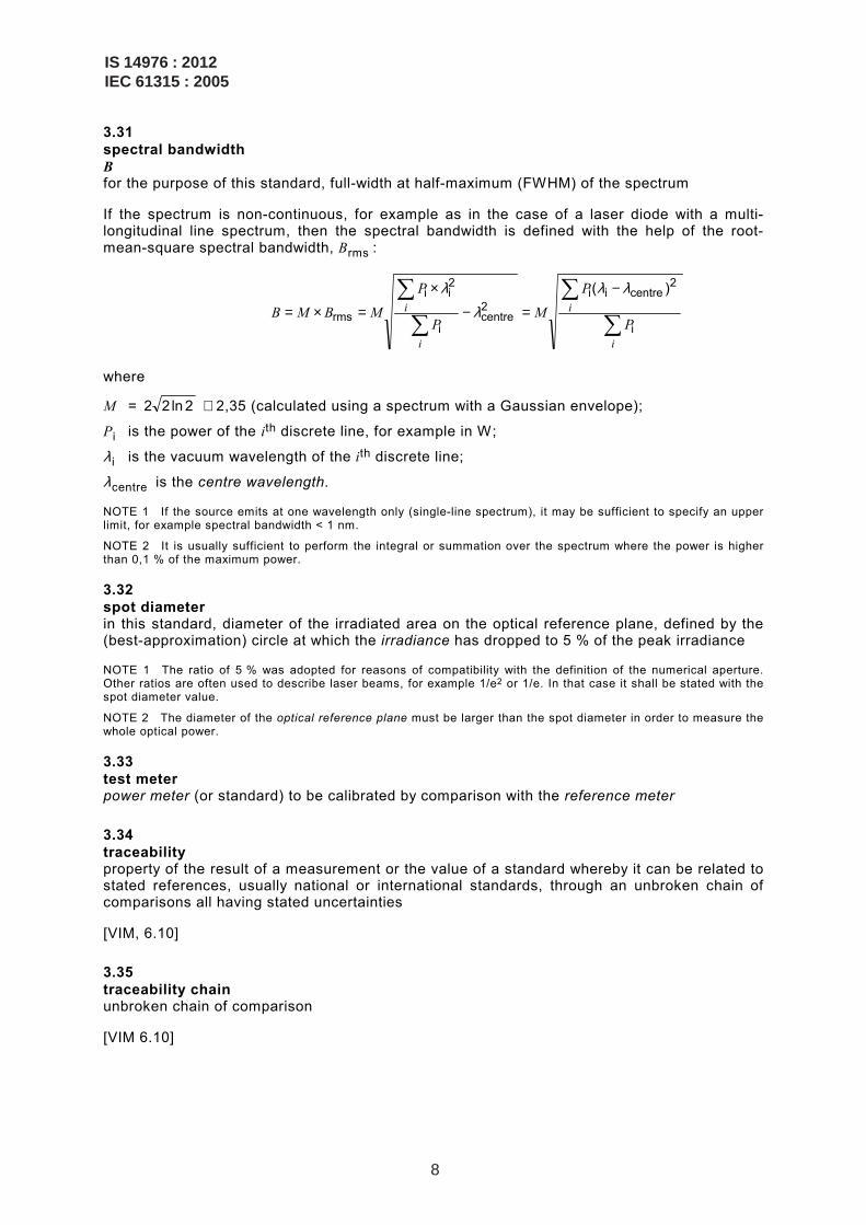
3.31 spectral bandwidth B for the purpose of this standard, full-width at half-maximum (FWHM) of the spectrum

If the spectrum is non-continuous, for example as in the case of a laser diode with a multi-longitudinal line spectrum, then the spectral bandwidth is defined with the help of the root-mean-square spectral bandwidth, Brms :

∑

∑∑

∑ −

=−

×

=×=

i

i

i

iP

PM

P

PMBMB

i

2centreii

2centre

i

2ii

rms

)( λλλ

λ

where

M = 2ln22 ≅ 2,35 (calculated using a spectrum with a Gaussian envelope);

Pi is the power of the ith discrete line, for example in W;

λ i is the vacuum wavelength of the ith discrete line;

λcentre is the centre wavelength.

NOTE 1 If the source emits at one wavelength only (single-line spectrum), it may be sufficient to specify an upper limit, for example spectral bandwidth < 1 nm.

NOTE 2 It is usually sufficient to perform the integral or summation over the spectrum where the power is higher than 0,1 % of the maximum power.

3.32 spot diameter in this standard, diameter of the irradiated area on the optical reference plane, defined by the (best-approximation) circle at which the irradiance has dropped to 5 % of the peak irradiance

NOTE 1 The ratio of 5 % was adopted for reasons of compatibility with the definition of the numerical aperture. Other ratios are often used to describe laser beams, for example 1/e2 or 1/e. In that case it shall be stated with the spot diameter value.

NOTE 2 The diameter of the optical reference plane must be larger than the spot diameter in order to measure the whole optical power.

3.33 test meter power meter (or standard) to be calibrated by comparison with the reference meter

3.34 traceability property of the result of a measurement or the value of a standard whereby it can be related to stated references, usually national or international standards, through an unbroken chain of comparisons all having stated uncertainties

[VIM, 6.10]

3.35 traceability chain unbroken chain of comparison

[VIM 6.10]

IS 14976 : 2012IEC 61315 : 2005

8

Nationalstandard

Transfer standard

Working standard

Workingstandard

Test Meter

National standards laboratory

Accredited calibration laboratory

Calibration laboratory of company

Figure 2 – Example of a traceability chain

3.36 working standard standard that is used routinely to calibrate or check measuring instruments

[VIM, 6.7]

NOTE A working standard is usually calibrated against a reference standard.

3.37 zero error measurement result of a power meter without irradiation of the optical input port

(VIM, 5.23)

4 Preparation for calibration

4.1 Organization

The calibration laboratory should satisfy requirements of ISO/IEC 17025.

There should be a documented measurement procedure for each type of calibration performed, giving step-by-step operating instructions and equipment to be used.

4.2 Traceability

The requirements of ISO/IEC 17025 should be met.

All standards used in the calibration process shall be calibrated according to a documented program with traceability to national standards laboratories or to accredited calibration laboratories. It is advisable to maintain more than one standard on each hierarchical level, so that the performance of the standard can be verified by comparisons on the same level. Make sure that any other test equipment which has a significant influence on the calibration results is calibrated. Upon request, specify this test equipment and its traceability chain(s). The re-calibration period(s) shall be defined and documented.

IS 14976 : 2012IEC 61315 : 2005

9

4.3 Advice for measurements and calibrations

This subclause gives general advice for all measurements and calibrations of optical and fibre-optic power meters.

The calibration should be made in a temperature-controlled room if non-temperature-controlled detectors are used. The recommended temperature is 23 °C. Humidity control may be necessary if humidity-sensitive optical detectors are used, or if there is the possibility of condensation on the components. A change of the laboratory's humidity may change the absorption of air and thereby change the power. This effect is relatively strong between 1 360 nm and 1 410 nm, especially when a sequential-type, open-beam calibration is used and the humidity changes between the steps. In parallel-type calibrations with open-beam paths of approximately the same lengths, the measurement results of both the reference meter and the test meter will change at approximately the same time, with negligible effect on the calibration result.

The laboratory should be kept clean. Connectors and optical input ports should always be cleaned before measurement. The quality and cleanness of the connector in front of the detector should be checked. All fibres should be moved as little as possible during the measurements; they can be fixed to the work bench if necessary. Sensors should be moved to the fibre rather than the fibre to the sensor.

The optical source which is used for the excitation of the power meter should be characterized for centre wavelength and spectral bandwidth. The spectral bandwidth should be narrow enough to avoid averaging over a wide range of wavelengths. Means to ensure the stability of the source, for example with the help of independent power monitoring, may be advisable.

Laser diodes are sensitive to back reflections. To improve the stability, it is advisable to use an optical attenuator or an optical isolator between the laser diode and the test meter. Because of their narrow spectral bandwidths, the combination of laser diode and multimode fibre is also capable of producing speckle patterns on the optical reference plane, with the result of an increased measurement uncertainty.

Fibre connectors and connector adapters are likely to produce errors in the measurement result [2], because of multiple reflections between the optical input port (or detector) and the connector-adapter combination (as part of the source). Therefore, connectors and adapters with low reflectivity are recommended for the calibration. Otherwise, a correction factor and an increased uncertainty may have to be taken into account.

It is advisable to use reference meters with detector diameters of ≥ 3 mm, because they can easily be irradiated with an open beam, and they are less susceptible to contamination (dirt and dust). The reference meter's surface reflections should be as small as possible. If the source emits a divergent beam, then a reference meter with an integrating sphere may be advisable. It is also acceptable to use meters with "flat" detectors and mathematical correction, based on multiplying the emitted far field distribution with the measured angle-dependence of the detector of the reference meter, and integrating over the range of far-field angles.

Temperature control of the detectors should be considered for highly accurate calibrations, because detectors exhibit strong temperature dependence over some wavelength ranges.

IS 14976 : 2012IEC 61315 : 2005

10

4.4 Recommendations to customers It is recommended that the customer (user of the power meter) maintain at least one reference power meter, which allows comparison of the meters for confidence. These comparisons are particularly important before and after the meter is sent to re-calibration, because they will allow the user to determine whether or not his scale has changed – for example due to transport – after the meter returns. Scale changes due to adjustment (see IEV 311-03-16 and VIM 4.30) will be reported on the calibration certificate.

A regular comparison of the correction factors, or of the deviations, will allow the user to screen out excessive ageing, and to possibly adjust the recalibration intervals.

5 Absolute power calibration

The calibration of a power meter is usually achieved by exposing both the meter under test and a calibrated power meter with known uncertainty (the reference meter) to an optical radiation, and by transferring the reference meter's measurement result to the test meter.

The allowable spectral bandwidth depends on the test meter's spectral responsivity; the stronger its wavelength dependence, the narrower the spectral bandwidth. Usual bandwidths are <15 nm, which excludes the possibility of calibrating with wider-bandwidth LEDs. Therefore, either laser diodes or combinations of "white" sources and narrow-bandwidth filters (for example monochromators) are typically used in optical power meter calibrations.

Depending on the type of source and the exciting beam geometry, four most frequent calibration methods can be distinguished:

Table 1 – Typical calibration methods and correspondent power

Radiation source Open-beam calibration Fibre beam calibration

"White" with filter P ≈ 10 µW P ≈ 10 nW to 0,3 µW (MM)

P ≈ 2 nW (SM)

Laser diode P ≈ 10 µW to 1 mW P ≈ 10 µW to 1 mW (SM and MM)

MM: multimode fibre (usually graded-index fibre)

SM: single-mode fibre

One can distinguish between the sequential and the parallel measurement method. When reference meter and test meter are sequentially exposed to the source, then the radiated power should be kept as constant as possible, for example by appropriate stabilization. For the parallel-type calibration, a beam splitter or a branching device is used to generate two beams which excite both the reference meter and the test meter simultaneously. In this case, the beam splitter or branching device ratio should be determined as accurately as possible, and its stability should be investigated.

As an example, a measurement setup for sequential, fibre-based calibration is illustrated in Figure 3. A launching device, for removal of the cladding modes and creation of an appropriate modal excitation, is included in the setup.

IS 14976 : 2012IEC 61315 : 2005

11

S dB

Attenuator (optional) Power meter

under test

Source Cladding mode

stripper

Reference power meter

Figure 3 – Measurement setup for sequential, fibre-based calibration

5.1 Establishing the calibration conditions

The calibration conditions are the measurement conditions during the calibration process. Establishing and maintaining the calibration conditions is an important part of the calibration, because any change of these conditions is capable of producing erroneous measurement results. The calibration conditions should be a close approximation to the intended operating conditions. This ensures that the (additional) uncertainty in the operating environment is as small as possible. The calibration conditions should be specified in the form of nominal values with uncertainties when applicable. In order to meet the requirements of this standard, the calibration conditions shall at least consist of:

a) the date of calibration; b) the ambient temperature with uncertainty, for example 23 °C ± 1 °C; c) the ambient relative humidity, if it has an influence, otherwise a relative humidity below the

condensation point is assumed; d) the nominal radiant power on the optical reference plane; e) the beam geometry:

1) an open (for example collimated) beam, described by the spot diameter on the optical reference plane, the beam's numerical aperture and the irradiance distribution in the beam. Typical irradiance distributions are: uniform, Gaussian or even irregular (speckled);

2) the type of fibre and, if applicable, its degree of excitation (for example fully excited); f) the connector-adapter combination: the connector type, polishing and adapter as part of the

exciting source (if applicable); g) the centre wavelength of the exciting source with its uncertainty; h) the spectral bandwidth of the exciting source with its uncertainty; i) the state of polarization: "unpolarized light" or "polarized light, undefinite state". If the latter

is chosen, the uncertainty due to polarization dependent response shall be taken into account in 5.3.2 and 5.3.4.

The above conditions may not be exhaustive. There may be other parameters which have a significant influence on the calibration uncertainty and therefore shall be reported, too.

In the calibration with an open-beam, the power meter's optical reference plane should be centrally irradiated with a beam diameter smaller than the active area of the optical reference plane.

IS 14976 : 2012IEC 61315 : 2005

12

In the calibration with a fibre, a single-mode fibre or a multimode fibre may be used. A single-mode fibre may be advantageous because of its reproducible beam characteristics, but may not be available for all wavelengths. If a multimode fibre is used, then full excitation is preferred because this excitation can be more easily reproduced. A launching device may be necessary to create the appropriate excitation. Note that multimode fibres will emit irregular beam patterns (speckle patterns) when driven by a laser diode; this will result in an increased calibration uncertainty. Optical power in the cladding (cladding modes) should be removed with an appropriate mode stripper or launching device, if necessary.

A connector-adapter combination should only be reported if the power meter is calibrated with a fibre, that is not with an open beam. It is recommended to use a combination of connector and adapter with sufficiently low reflections back to the power meter.

5.2 Calibration procedure (1) Establish and record the appropriate calibration conditions (5.1). Switch on all

instrumentation and wait for enough time to stabilize. (2) Set up the instrument state of the reference meter and test meter according to the

instruction manual. Set the wavelength on all instruments for the source wavelength. Select appropriate power ranges. Record the instrument states of both meters. Adjust the zero of both meters if applicable.

(3) Measure the optical power with the reference meter Pstd,1. Multiply the measurement result by the correction factor of the reference meter CFstd reported in its calibration certificate if it has not been adjusted. Multiply by the correction factor CFchange calculated in 5.3.3 if necessary. Record the measurement result, Pref,1 = Pstd,1 x CFstd x CFchange. This is the best estimate of the true power.

(4) Measure the optical power with the test meter. Apply necessary corrections as suggested by the operating instructions. Record the measurement result, PDUT,1.

(5) Calculate the first of a series of correction factors:

DUT,1

ref,11,comparison P

PCF = . (1)

(6) Repeat steps (3) through (5) several times, with the result of obtaining several correction factors, CFcomparison,1 to CFcomparison,n.

(7) Calculate and record the average correction factor, CFDUT from the individual correction factors:

∑=

⋅=n

iCF

nCF

1i,comparisonDUT

1 (2)

If desired the deviation D can be calculated from the correction factor:

11

DUT−=

CFD (3)

In later use of the test meter, the measurement results shall be multiplied with CFDUT. Alternatively, an adjustment of the test meter can be made so that the correction factor is changed to 1. In this case, the comparison should be repeated for verification.

IS 14976 : 2012IEC 61315 : 2005

13

5.3 Calibration uncertainty

The calibration uncertainty is the measurement uncertainty of the correction factor CFDUT. Calculate the combined standard uncertainty from:

2DUT

2ref

2setupDUT uuuCFu ++=)( (4)

where

usetup = uncertainty due to the setup, (5.3.1);

uref = uncertainty of the reference meter, (5.3.2);

uDUT = uncertainty due to the test meter, (5.3.4).

NOTE Equation (4) is valid only if the input quantities are independent or uncorrelated. If some input quantities are significantly correlated, the correlation must be taken into account. See GUM for more detail.

Then calculate the expanded uncertainty from:

)()( DUTDUT CFukCFU ×= , (5)

where k is the coverage factor. See Annexe A for more detail.

5.3.1 Uncertainty due to the setup

The following uncertainties may come from the setup.

a) Uncertainty due to the source power instability. In addition to the intrinsic variation of output power versus time, a laser source may react with unstable power to variations of back-reflections and variations of the state of polarisation of back-reflected light.

b) Uncertainty due to the beam splitter or branching device ratio (for parallel method), for example due to their polarization dependence.

c) Depending on the setup and method, other uncertainties may have to be taken into account.

Instability of the source power, of the beam splitter or branching device ratio (for parallel method) will cause a scatter in the measurement of the correction factor. The uncertainty due to these instabilities can be calculated from the experimental standard deviation of the correction factors CFcomparison,1 to CFcomparison,n measured during the calibration (Equation (1)). The number of comparisons should be large to reduce this uncertainty. See Annex A for more detail on type A evaluation of uncertainty.

n

CFsu

)( comparisontypeAsetup, = (6)

where: s(CFcomparison) is the experimental standard deviation of the correction factors;

n is the number of measurement cycles during the calibration process.

IS 14976 : 2012IEC 61315 : 2005

14

This uncertainty can also be calculated from a standard deviation evaluated once from measurements and used for all calibrations or from a type B evaluation. The instability should therefore not vary too much from one calibration to the next and not depend on the test meter. The number n in Equation (6) is always the number of measurement cycles during the current calibration process.

This type A evaluated uncertainty will also be influenced by the repeatability of the connection when using a sequential measurement method or by slight changes in the measurement conditions during the calibration process. It can (partially) take into account some of the uncertainties due to the reference meter (5.3.2) or test meter (5.3.4). Uncertainty components should not be taken twice into account but also not be forgotten.

Calculate the uncertainty due to the setup by combining all partial uncertainties described in this subclause:

∑=

=m

iuu

1

2isetup,setup (7)

5.3.2 Uncertainty of the reference meter

The uncertainty of the reference meter is mainly due to its calibration, to the uncertainties of the current calibration conditions and to the dependence of the reference meter on these conditions.

The following uncertainties shall be evaluated. The evaluation can be made on the basis of measurements or estimations, or a mixture of both. The calculation of uncertainties is described in Annex A. The measurement of dependence on conditions is described in 6.2.1.

a) calibration uncertainty of the reference meter. It shall be obtained from its calibration certificate;

b) uncertainty due to the change from the conditions in which the reference meter was calibrated and the current calibration conditions uchange as calculated in 5.3.3;

c) uncertainty due to temperature dependence of the reference meter; d) uncertainty due to dependence on relative humidity of the reference meter. Power meters

with integrating sphere are particularly sensitive to absorption peaks of water when using narrow laser sources;

e) uncertainty due to dependence on the beam geometry of the reference meter; f) uncertainty due to dependence on multiple reflections. Multiple reflections may exist

between the optical input port and the radiation source (for example a connector-adapter combination). Different artefacts will change the measured power;

g) uncertainty due to wavelength dependence of the reference meter; h) uncertainty due to dependence on source spectral bandwidth of the reference meter; i) uncertainty due to dependence on state of polarization of the reference meter, except if

unpolarized or depolarized light is used for calibration; j) uncertainty due to optical interference. Fabry-Perot cavities can occur between the surface

of the detector, of the window and the end of the connector, if used;

IS 14976 : 2012IEC 61315 : 2005

15

k) uncertainty due to the resolution of the reference meter. If the resolution of the reference meter is δyref, the standard uncertainty is (see GUM, F.2.2.1):

refresolutionref,32

1 yu δ= (8)

l) uncertainties due to other dependences of the reference meter. Depending on the type of reference meter, there may be other uncertainties of the reference meter. These should also be measured or estimated.

Note that ageing is considered as a change of condition, with the time being the influencing condition. The elapsed time ∆t between the calibration of the reference meter and its usage in the calibration of the test meter is known and its uncertainty is u(∆t) = 0. The uncertainty due to ageing of the reference meter is calculated in 5.3.3.1 and is taken into account in point b).

Then calculate the combined standard uncertainty of the reference meter from the n above standard uncertainties:

2change

1

2iref,ref uuu

n

i+= ∑

= (9)

where uchange is the uncertainty due to the change of conditions, as determined from 5.3.3.

5.3.3 Correction factors and uncertainty caused by the change of conditions

The reference meter may exhibit a different response because it was calibrated under conditions different from the current calibration conditions. Examples for differences between the two sets of measurement conditions are: Parallel beam versus divergent beam, different source spectra, a non-reflecting setup versus a setup with multiple reflections, or a large time span between the two reference dates resulting in ageing of the standard.

If the conditions under which the reference meter was calibrated are nominally identical to the current calibration conditions (their uncertainties can be different) and if the ageing of the reference meter is negligible, this clause can be skipped (CFchange = 1).

As indicated in Figure 4, each change comprises the nominal change of condition and the change of uncertainty.

IS 14976 : 2012IEC 61315 : 2005

16

Condition in which the reference was calibrated (“previous” condition)

“Current” measurement condition

Nominal change of condition (generates the correction factor)

"Previous” uncertainty

"Current” uncertainty

"Current" uncertainty ifcorrection factor = 1

Alternative A

Alternative B

Figure 4 – Change of conditions and uncertainty

For each of the potential error contributions (5.3.3.1 to 5.3.3.8) one should decide if it is sensible to calculate a correction factor or not. Alternative A includes the calculation of a correction factor with the result of a relatively small uncertainty. Alternative B means waiving the correction factors (or CFchange = 1) and taking larger uncertainties into account to embrace the worst-case conditions.

If the alternative A is chosen, the (cumulative) correction factor is:

current

previouschange r

rCF = (10)

or rCF ∆−= 1change (11)

where

rprevious is the response of the reference with excitation at the conditions at which it was calibrated;

rcurrent is the response of the reference with excitation at the current calibration conditions;

∆r is the relative change of response ∆r = (rprevious – rcurrent) / rcurrent.

Calculate the (cumulative) reference meter's change-related correction factor by accumulating the partial correction factors, CFchange,i , outlined in 5.3.3.1 to 5.3.3.8. For each influencing quantity Xi, start with the calculation of the partial correction factor:

iichange, 1 rCF ∆−= (12)

IS 14976 : 2012IEC 61315 : 2005

17

The relative change of response ∆ri can be directly measured by changing the influencing quantity from the “previous” to the “current” calibration conditions or calculated from the nominal change of the influencing quantity ∆xi, and the reference meter's nominal relative dependence on this quantity:

iiichange, 1 xcCF ∆×−= (13)

where ci is the partial derivate of the relative response on the influence quantity Xi, called sensitivity coefficient:

i0

i xr1

∂∂=

rc (14)

If the sensitivity coefficient is not known very well, the following type B uncertainty has to be taken into account:

iiichange, )( xcuu ∆×= (15)

where u(ci) is the standard uncertainty of the sensitivity coefficient. The measurement of the dependences is discussed in 6.2.

Finally, calculate the reference meter's cumulative correction factor from the above contributions:

ichange,1

change CFCFn

i=Π= (16)

and the combined standard uncertainty due to the change of calibration conditions:

∑=

=n

iuu

1

2ichange,change (17)

This correction factor corresponds to a known change of response of the reference meter caused by the two different sets of measurement conditions. It is a correction factor to apply to the power read by the reference meter (see 5.2).

5.3.3.1 Ageing

As mentioned in 5.3.2 the ageing is a change of condition. A correction factor is usually not calculated (CF = 1) except if the ageing coefficient of the reference meter is well known and stable and over a long time. The uncertainty should be calculated by multiplying the elapsed time ∆t between the calibration of the reference meter and its use in the calibration of the test meter with the reference meter's ageing coefficient uncertainty u(ct).

tcuu ∆×= )( ttchange, (18)

Example: Only limits of ageing are known: ± 0,1 %/year. Following annex A, the ageing coefficient is ct = 0 %/year and its uncertainty u(ct) = 0,1/ 3 %/year.

The uncertainty due to ageing of the reference meter one year after its calibration is then

=∆×= tcuu )( ttchange, 0,1/ 3 %/year x 1 year = 0,06 % (19)

IS 14976 : 2012IEC 61315 : 2005

18

5.3.3.2 Correction factor due to temperature change

The correction factor CFchange,Θ should be calculated with the help of the nominal change between the "previous" and the "current" temperature ∆Θ and the temperature sensitivity coefficient cΘ of the reference meter (for example in %/°C).

∆Θ×−= ΘΘchange, 1 cCF (20)

5.3.3.3 Correction factor due to change of power level

The uncertainty should be calculated from the nonlinearity of the reference meter between the "previous" and the "current" power level. If necessary, a correction factor can be calculated from:

10NLchange, 10

NL

CF−

= (21)

where NL is the nonlinearity, expressed in decibels (dB). Measurement of nonlinearity is described in Clause 7.

5.3.3.4 Correction factor due to change of beam geometry

The correction factor should be calculated from the change of response measured when changing the beam geometry.

5.3.3.5 Correction factor due to dependence on multiple reflections

The reference meter's optical input port should generally be assumed to be reflective. Such a reflection will travel back to the radiation source, be reflected again, and finally increase the displayed optical power level. This effect will give rise to a correction factor (usually < 1) and an increased uncertainty.

If, for example, the source used in the calibration of the reference meter was non-reflective and the source used in the calibration of the test meter is reflective (caused by an optical connector), then the total power indicated by the reference meter is erroneous by the secondary reflection. If one assumes that the secondary reflection contributes an additional 5 % of the total power, then the individual correction factor is 0,95. This type of error can be reduced by using sources with highly absorptive enclosures, respectively sources with low-reflectivity connector-adapter combinations.

5.3.3.6 Correction factor due to wavelength change

The correction factor should be calculated with the help of the nominal change of wavelength ∆λ and the reference meter's nominal wavelength dependence cλ .

λλλ ∆×−= cCF 1change, (22)

5.3.3.7 Correction factor due to spectral bandwidth change

The correction factor should be calculated with the help of the nominal change of spectral bandwidth and the reference meter's nominal dependence on the spectral bandwidth. Note that the correction factor remains 1 as long as the (uncorrected) wavelength-dependence is linear within the spectral bandwidth of the source. In the case that the wavelength dependence is

IS 14976 : 2012IEC 61315 : 2005

19

curved, the correction factor can be computed with the help of the wavelength-dependence of the reference meter and the spectra of the two sources used in the calibration of the reference meter and in the calibration of the test meter.

5.3.3.8 Other correction factors

Depending on the type of reference meter and the calibration conditions, there may be other correction factors. These should also be measured or estimated as outlined above.

5.3.4 Uncertainty due to the test meter

Uncertainties arising from the test meter are mainly due to the uncertainties of the calibration conditions and the dependence of the test meter on the conditions. The following uncertainties shall be evaluated. Their determination is similar to 5.3.2. The calculation of uncertainties is described in Annex A, the measurement of dependence on conditions is described in 6.2.1.

a) Uncertainty due to temperature dependence of the test meter. b) Uncertainty due to dependence on relative humidity of the test meter. Power meters with

integrating sphere are particularly sensitive to absorption peaks of water when using narrow laser sources.

c) Uncertainty due to dependence on beam geometry. This uncertainty comes from non-uniformity and angle-dependence of the test meter's optical input port.

d) Uncertainty due to dependence on multiple reflections. Multiple reflections may exist between the optical input port and the radiation source (for example a connector-adapter combination). Different artefacts will change the measured power.

e) Uncertainty due to wavelength dependence of the test meter. f) Uncertainty due to dependence on source spectral bandwidth of the test meter. g) Uncertainty due to dependence on state of polarization of the test meter, except if

unpolarized or depolarized light is used for calibration. h) Uncertainty due to optical interference. Fabry-Perot cavities can occur between the surface

of the detector, of the window and the end of the connector, if used. i) Uncertainty due to the resolution of the test meter. If the resolution of the test meter is

δyDUT, the standard uncertainty is (see GUM, F.2.2.1):

DUTresolutionDUT,32

1 yu δ= (23)

j) Uncertainties due to other dependences of the test meter. Depending on the type of test meter and on the calibration process, there may be other conditions causing uncertainties.

Then calculate the combined standard uncertainty contribution of the test meter from the n above standard uncertainties:

∑=

=n

iuu

1

2iDUT,DUT (24)

IS 14976 : 2012IEC 61315 : 2005

20

5.4 Reporting the results

The results of each calibration should be reported as required by ISO/IEC 17025. Calibration certificates or calibration reports referring to this standard shall at least include the following information:

a) all calibration conditions as described in 5.1; b) the test meter's correction factor(s) or deviation(s), if the test meter was not adjusted;

c) on receipt correction factors or deviations and after adjustment correction factors or deviations in the case that an adjustment was carried out;

d) the calibration uncertainty in the form of an expanded uncertainty as described in 5.3; e) the instrument state of the test meter during the calibration; f) evidence that the measurements are traceable (see ISO/IEC 17025:1999, 5.10.4.1 c)).

6 Measurement uncertainty of a calibrated power meter

The measurement uncertainty of a calibrated power meter is greater than its calibration uncertainty. It is the combination of the calibration uncertainty and of uncertainty contributions due to the dependence of the power meter on the conditions of measurement.

The determination of the measurement uncertainty of a calibrated power meter used at reference conditions or at operating conditions is not part of the calibration process. It is performed for example by manufacturers of power meters in order to establish specifications. It is not mandatory for calibration certificates or calibration reports referring to this standard.

6.1 Uncertainty at reference conditions

Reference conditions are used for testing the performance of a power meter or for intercomparisons. They are usually defined by manufacturers in order to specify the smallest uncertainty of a measuring instrument; therefore they are often identical or close to its calibration conditions.

The uncertainty at reference conditions is the uncertainty on the result of a measurement taken by the calibrated and adjusted power meter when operated at reference conditions. It depends on the calibration uncertainty of the power meter, the reference conditions and the dependence of the power meter on the reference conditions. This is the reason why the uncertainty at reference conditions is always larger than the calibration uncertainty. Even when the reference conditions are identical with the calibration conditions (no uncertainty due to change of conditions), the test (power) meter’s dependences on the reference conditions have to be added (in quadrature) to the calibration uncertainty for a second time. Calculating the uncertainty at reference conditions of the calibrated test meter is similar to calculating the measurement uncertainty at calibration conditions of the reference meter described in 5.3.2:

2DUTDUT

2ionsref_conditDUT, uCFuu += )( (25)

where

u(CFDUT) is the calibration uncertainty of the test meter, as determined from 5.3, and

uDUT is the uncertainty due to the dependence of the test meter on the reference conditions, as determined from 5.3.4.

The description of the reference conditions should be made in the same way as the calibration conditions described in 5.1.

IS 14976 : 2012IEC 61315 : 2005

21

6.2 Uncertainty at operating conditions

The uncertainty at operating conditions (or operating uncertainty, see 2.2.11 of IEC 60359) is the uncertainty on the result of a measurement taken by the calibrated and adjusted power meter when operated within a range of operating conditions. It depends on the calibration uncertainty, the operating conditions and the dependence of the power meter on the operating conditions:

2extensionDUT

2operatingDUT, uCFuu += )( (26)

where

u(CFDUT) is the calibration uncertainty of the test meter, as determined from 5.3, and

uextension is the extension uncertainty, due to the dependence of the meter on the operating conditions, as determined from Equation (27).

On the contrary to the calibration conditions described in 5.1, each operating condition should be described by a range when possible. The set of operating conditions are specified by:

a) the maximum time span between recalibrations; b) the range of ambient temperatures; c) the range of power levels (measuring range); d) the range of beam geometries described by their spot diameter and numerical aperture, or

the range of fibre types; e) the applicable connector-adapter combinations, if any; f) the range of wavelengths of the source; g) the maximum spectral bandwidth of the source.

All possible polarization states are included in the operating conditions by default. A relative humidity below the condensation point is also assumed.

The above conditions may be defined either by the power meter manufacturer or by the calibration laboratory in charge of the calibration for operating conditions.

To calculate the extension uncertainty, combine all uncertainties due to the dependences on the conditions:

∑=

=n

iuu

1

2iextension,extension (27)

where:

uextension,i are contributions to the extension uncertainty;

n is the total number of contributions.

6.2.1 Determination of dependences on conditions

Each individual dependence should be recorded as relative change of the meter's response, caused by changing the relevant condition within its operating range. During the test, all other conditions should be kept at the calibration conditions. The zero point is defined by the response at calibration conditions. This way, each dependence can be specified by a range which is defined by the maximum positive and negative changes of the response. An asymmetric range about the zero-point is the usual result as shown in Figure 5.

IS 14976 : 2012IEC 61315 : 2005

22

Operating condition

Specified range of operating parameter

∆r (%)

Calibrationcondition

Actual set of limits

0

Dependence on operating condition

xi

Figure 5 – Determining and recording an extension uncertainty

In order to obtain good measurement accuracy, the guidelines in Clause 4 should be observed. Uncertainties in the measurements should be as small as possible, because the measurement results shall include these uncertainties. It is acceptable to use estimations, instead of measurements, if these estimations are based on known physical relations or on a sufficiently large number of characterizing measurements of the same type of test meter.

For the determination of the combined standard uncertainty of the test meter at operating conditions, the limits quantifying the individual dependences shall be converted to standard uncertainties using Equation (A.6).

The individual uncertainties are usually assumed to be independent. However, in some instances an uncertainty may be strongly dependent on more than one condition. Examples are outlined in 6.2.4, 6.2.6 and 6.2.7. If the extension uncertainty is substantially increased by changing the other conditions (within their specified operating ranges), then this larger uncertainty shall be recorded. The calculation of the uncertainty shall then be based on these larger uncertainties.

6.2.2 Ageing

Ageing is the relative change of response during a period. It can be determined from the results of successive calibrations of the meter at the same conditions or from indications of the manufacturer.

For a manufacturer, the relative change of response during a period shall be determined with the assumption of careful use of the instrument. It is recommended to expose the power meter to its typical environmental conditions, for example ambient temperature (23 ± 1) °C for a laboratory-type instrument, optical input port non-irradiated, continuously repetitive cycles of power-on 12 hours, power-off 12 hours, with a total test time equal to the period. The change of response should be measured by comparison with a working standard. Regular and traceable recalibration of the working standard will be necessary, in order to exclude ageing of the working standard. As always, the measurement uncertainty, in this case mostly the uncertainty of the working standard, shall be taken into account.

It is recommended to calculate the ageing uncertainty from a rectangular distribution obtained as described above (see Clause A.2). If, for example, a detector is known to increase its response by a maximum of 0,1 % per year at a certain wavelength, then the ageing uncertainty is characterized by a rectangle which extends from 0 % (at time 0) to +0,1 % (at time 1 year).

IS 14976 : 2012IEC 61315 : 2005

23

6.2.3 Dependence on temperature

The relative change of response against the response at the calibration conditions should be measured by changing the temperature within the operating temperature range. The rectangular uncertainty distribution is then defined by the most negative and the most positive relative changes of the response. Only the extremes of the response as function of the temperature are relevant, not the responses at the extremes of the temperature (see Figure 5).

Note that the temperature dependence of the spectral responsivity of semiconductor detectors depends on the wavelength.

6.2.4 Dependence on the power level (nonlinearity)

The relative change of response against the response at the calibration power level should be measured following Clause 7.

6.2.5 Dependence on the type of fibre or on the beam geometry

Fibre-optic power meters may be designed to accept fibres or open beams. It is assumed that the response of the power meter depends on the geometry of the light beam because, for example, of non-uniformity and angle-dependence of the meter's optical input port.

The relative change of response should be measured with a working standard that exhibits:

− negligible angle-dependence,

− negligible surface reflections, and

− a sufficiently large active area to capture the fibre beams or the open beams.

A good choice of working standard may be a well-characterized power meter with an integrating sphere.

Figure 6 – Possible subdivision of the optical reference plane into 10 x 10 squares, for the measurement of the spatial response

Active area of opticalreference plane

(10 × 10) squares

IS 14976 : 2012IEC 61315 : 2005

24

Another possibility is evaluating the uncertainties with a mathematical analysis, based on the assumption that all uncertainties are caused by non-uniform spatial responses of the test meter's reference plane. In preparation of this, the active area of the optical reference plane should be subdivided into an array of squares, for example 10 x 10 squares as in Figure 6.

Then two types of measurements should be carried out:

a) measurements of the spatial power density, together with the angles of incidence, on the optical reference plane as generated by the applicable beam geometries;

b) measurements of the test meter's spatial response, weighted with appropriate multipliers which characterize the meter's dependence on oblique incidence (angle dependence), on the test meter's reference plane. The spatial response should be measured with a beam diameter equal to the length of the square.

The change of response upon changing the beam parameters can then be evaluated on the basis of modelling the necessary measurement results, by multiplying the (spatial) power levels with the spatial responses and adding all products. Note that the spatial responses are usually wavelength-dependent.

6.2.5.1 Measurement of the fibre dependence

In the test of fibre-related uncertainties, the fibres under test should be fully excited, both in terms of the core diameter and of the numerical aperture. An approximate fibre length of 2 m is recommended. Optical power in the cladding (cladding modes) should be removed with appropriate mode strippers if necessary. The fibres should be terminated by the connector-adapter combination defined by the calibration conditions. Both the connector and the adapter should exhibit a low reflectivity, so that multiple reflections between the connector-adapter combination and the detector do not influence the measurement results. The spectral bandwidth of the source should be narrow enough to avoid averaging over a wide range of wavelengths.

Step 1: the output of the reference fibre is measured with both the working standard and the test meter, and the difference is (mathematically) adjusted to zero.

Step 2: the above procedure is applied to:

a) a standard single-mode fibre as defined by IEC 60793-2, and b) the (specified) fibre with the largest core diameter, the fibre with the largest

numerical aperture or both.

The intention of the test is to measure the dependence of the test meter on the type of fibre and on the mode volume. The largest relative change of response against step 1 (positive and negative) should be used to determine the fibre-related uncertainty. The uncertainty shall also include the uncertainty in measuring the fibre outputs with the working standard, caused for example by the effects of non-uniformity, beam divergence and multiple reflections on the working standard.

In these measurements, a significant type A uncertainty may be caused by "speckles", in conjunction with the non-uniformity of the optical input port. Speckles are irregular irradiance distributions which are caused by interference between different modes in a multimode fibre. This effect occurs particularly when the fibre is excited by the (highly coherent) radiation from a laser diode. This uncertainty can be reduced by averaging a series of measurement results, in which each sample is taken after a slight movement of the fibre. Fibre movement will change the speckle pattern. Note this may be accompanied by a change of the total radiant power, because of a change of the reflected power and the laser diode sensitivity to reflected power.

IS 14976 : 2012IEC 61315 : 2005

25

Speckles do not exist in single-mode fibres when the exciting wavelength is sufficiently longer than the fibre's cut-off wavelength. Another possibility of eliminating the speckle pattern is using a less coherent source, such as an LED or (filtered) "white" radiation source.

6.2.5.2 Measurement of open-beam dependence

Similar to measuring the fibre dependence, the dependence on the spot diameter and the numerical aperture of an open beam can be evaluated by comparison with a working standard which exhibits a uniform large area detector and negligible angle dependence.

To address the problem of combined dependence on spot diameter and numerical aperture, it may be sufficient to evaluate:

a) the relative change of response (against the response at calibration conditions) due to excitation with the specified smallest spot diameter – smallest numerical aperture; and

b) the relative change of response due to excitation with the specified largest spot diameter- largest numerical aperture.

6.2.6 Dependence on the connector-adapter combination

This subclause discusses the test meter's dependence on multiple reflections between the optical input port and the radiation source (for example an optical connector or other mechanical parts in the beam path between the source and the optical input port). Note that the reflections may be specular or diffuse.

The relative change of response should be measured with the help of a working standard which exhibits negligible angle-dependence and surface reflections. The fibre should be the one of the calibration conditions. It is advisable to hold the fibre end in place during the measurement, in order to avoid any bending-induced changes of the power level.

Step 1: the reference beam geometry (respectively the reference fibre), together with the reference connector-adapter combination, is measured with both the working standard and the test meter, and the difference is (mathematically) adjusted to zero.

Step 2: the above procedure is applied to all specified connector-adapter combinations, by repeating each connection several times to reduce type A uncertainties. The largest relative change of response against step 1 (positive and negative) should be used to determine the uncertainty. The uncertainty shall also include the type B uncertainty in measuring the various combinations with the working standard, caused for example by multiple reflections on the working standard.

Referring to the last paragraph of 6.2.1, it may be necessary to additionally measure the dependence with the highest-order fibre, as listed in 6.2.5.1. A high-order fibre will create a larger image on the optical reference plane, and therefore make limitations in the positioning accuracy more obvious. In this case, an increased dependence should be recorded.

IS 14976 : 2012IEC 61315 : 2005

26

6.2.7 Dependence on wavelength

The relative change of spectral response against the response at the calibration wavelength should be measured. These measurements will normally be carried out using a spectrally continuous source imaged through a spectrally discriminating instrument, for example a monochromator or a number of spectral filters. The stray light, that is light not at the selected wavelength, should be evaluated, in order to ensure accurate measurement results. The centre wavelength(s) and the spectral bandwidth(s) should also be measured. The bandwidth should be narrow, because a wide bandwidth in conjunction with a strong curvature of the test meter's wavelength dependence is capable of producing erroneous measurement results. Note that extremely narrow spectral bandwidth may cause optical interference problems, that is comb-like wavelength dependence, when the beam path contains one or more optical resonators.

The beam geometry should be one of the calibration conditions. It may be possible to substitute a fibre beam using a combination of lenses and apertures. In this case, care should be taken to match the irradiated spot diameter and position on the optical reference plane with those achieved using a fibre input. Care should also be taken to ensure that back reflections from the optical input port do not add uncertainties to the measurement results.

The measurement should be carried out by direct comparison with a working standard by using the substitution technique. The working standard should have been calibrated for relative spectral response.

Because of the relatively low power levels in these measurements, zero adjustment of both power meters is essential. If the instrument comprises means of correction, for example a calibration curve or a table stored in a memory, the relative change of response from the corrected response has to be measured.

Changing the temperature may strongly influence the wavelength-dependence. For example, the wavelength-dependence of a germanium photodiode at 1 550 nm is much stronger at 0 °C than at room temperature. In general, the wavelength uncertainty shall be calculated on the basis of the largest wavelength-dependence, in this case the one at 0 °C.

6.2.7.1 Dependence on wavelength due to Fabry-Perot type interference

When using a narrow spectral bandwidth laser (B << 1 nm), the spectral response can sometimes vary rapidly with respect with wavelength as depicted in Figure 7. This is usually caused by Fabry-Perot cavity(ies) in the optical path to the detector. Fabry-Perot cavities can occur between the two faces of the window in the detector cap, between one face of the window and the detector itself, or, if a fibre is used, between the end of the fibre and any of the other surfaces.

IS 14976 : 2012IEC 61315 : 2005

27

0,000,050,100,150,200,250,30

1 535 1 540 1 545 1 550 1 555 1 560

Wavelength nm

Rel

ativ

e re

spon

se

dB

Figure 7 − Wavelength dependence of response due to Fabry-Perot type interference

In Figure 7, the peak-to-peak variation reaches ∆dB = 0,2 dB (∆% = 4,6 %) which is very important. The standard uncertainty due to optical interference is the standard deviation of the sine pattern.

%6,122

1 %int =

∆×=u (28)

6.2.8 Dependence on spectral bandwidth

This dependence increases with the curvature of the detector's wavelength dependence. The relative change of response as a function of the spectral bandwidth of the source has to be tested within the specified range of spectral bandwidths. A monochromator can be used to generate a variable spectral bandwidth; the actual power level should be measured with a working standard with negligible wavelength-dependence. The spectral-bandwidth dependence can also be evaluated by mathematical analysis, based on the known spectral response of the test meter and on the known spectral characteristics of the source.

6.2.9 Dependence on polarization

A method of evaluation of the polarization dependent response (PDR) of the test meter is to measure the response of the meter multiple times at different states of polarization. A stable light source polarized to nearly 100 % should be used, otherwise use a polarizer after the source as shown in Figure 8. A polarization controller is used to convert the fixed input polarization state to all possible output states.

S

Power meterSource Polarization

controller Polarizer

Figure 8 – Measurement setup of polarization dependent response

The source power instability and the loss variation of the polarization controller should be far smaller than the polarization dependence of the test meter. This should be verified by replacing the test meter with a detector with very low polarisation dependent response.

IS 14976 : 2012IEC 61315 : 2005

28

NOTE The laser sources may react with unstable power when light with varying polarization state is back-reflected, therefore an attenuator or isolator may have to be inserted between the source and the polarization controller.

Another PDR measurement method, the matrix method, can be adapted from the polarization dependent loss (PDL) measurement method in IEC 61300-3-12, as described in [3].

6.2.10 Other dependences

Depending on the type of test meter, there may be dependences on other parameters. These should also be characterized as relative changes of response against the response at the calibration conditions.

One example may be including intensity-modulated optical signals into the operating conditions, in the form of specifying a range of modulation frequencies and duty cycles, and evaluating the type B uncertainty due to the modulation. Be aware that extreme duty cycles are capable of saturating the detector, the electronics or both.

7 Nonlinearity calibration

The nonlinearity of the power meter should be calibrated to ensure accurate measurements at power levels away from the calibration level and for relative measurements such as loss and gain measurements. The calibration should be made by increasing and decreasing the power level to detect nonlinearities at the boundaries of each amplifier range or, whenever possible, to include measurement results at both sides of each range boundaries, in order to include nonlinearities at these boundaries. Be aware that the detector nonlinearity is dependent on the wavelength. As an example, an InGaAs detector that is linear at 1 310 nm and 1 550 nm may be nonlinear at 850 nm.

Several methods are possible. The superposition method is the reference method, as it is the most accurate and does not require a reference standard (self-calibrating method). However, the used power steps of 2 (about 3 dB) might be too large to detect nonlinearities that might appear at amplifier range boundaries. This limitation may be avoided by starting the calibration from several reference powers, or by taking separate measurements of the same power level on both sides of the amplifier range boundaries.

All methods use sources with selectable power level, for example (stabilized) laser diode sources and variable attenuators. The generated power levels should cover the specified measuring range. During the test, the maximum permissible irradiance of the input port should be defined by the optical power at the upper end of the measuring range and by single-mode fibre excitation.

The power level saturating the detector is dependent on the beam geometry. A small spot diameter may saturate the detector at lower power than a larger spot diameter.

NOTE Extreme ambient temperatures may increase the nonlinearity. Referring to the statement on "dependence on more than one operating condition" in 6.2, it may be necessary to additionally measure the nonlinearity at the extremes of the operating temperature range, and to record an increased uncertainty at operating conditions.

IS 14976 : 2012IEC 61315 : 2005

29

7.1 Nonlinearity calibration based on superposition

Highly accurate nonlinearity calibration is possible with the superposition method (also known as the addition method). A “fibred” version of the open-beam double aperture method [6] may be used with single-mode fibres. A possible setup is illustrated in Figure 9. The power is split into two different paths where shutters are located and then recombined on the power meter under test.

Power meterunder test

Reference power meter

dB

dB

AttenuatorSource Branching

device dB

Attenuator

Attenuator

Shutter

Shutter

S

Branching device

Figure 9 – Nonlinearity calibration based on superposition

Stable, optically-isolated (to reduce sensitivity to reflections) DFB lasers can be used, provided that the linewidth is broadened to yield an optimized coherence, as with the procedure for the absolute calibration. The two paths of the setup should have different lengths (around 100 m for DFB lasers) to avoid (Mach-Zehnder-type) interference fluctuations, and unused branches of branching devices must be terminated. The drawback of this method is its higher insertion loss: typically around 1,5 dB for the first attenuator, 0,5 dB for the first branching device, 1,5 dB for the second attenuators and about 3,5 dB for the combining branching device for a total of about 7 dB. For higher power measurements, an optional optical amplifier (like an EDFA for the 1,55 µm band) can be inserted between the source and the first attenuator.

7.1.1 Procedure (1) Set the attenuators in the two paths so that the power measured on the meter is the same

when light is coming from one path or from the other path. (2) Open both shutters and measure the total power from both paths simultaneously: Pab,i.

(3) Close the shutter on path b and measure the power from the path a: Pa,i.

(4) Close the shutter on path a, open the shutter on path b and measure the power from the path b: Pb,i.

(5) If the sum of the individual powers is not equal to the total power, there is a nonlinearity:

ib,ia,

iab,10i log10

PPP

NL+

×= (dB) (29)

(6) Using the first attenuator, attenuate the total power by a factor 2 (10 log10 2 ≅ 3,01 dB) to the level of the individual powers of the preceding step.

IS 14976 : 2012IEC 61315 : 2005

30

(7) Repeat steps (2) to (6) through all the desired range. (8) At the end, the global nonlinearity is the sum of all the local nonlinearities expressed in

decibels (dB), starting calculations from the reference power level where the nonlinearity is zero (higher order terms are neglected).

∑+

=−=

1

0inglobal )(

n

iNLPNL for n = –1, –2, –3, etc. (30)

0)( 0global =PNL (reference power)

∑=

+=n

iNLPNL

1inglobal )( for n = 1, 2, 3, etc.

where n < 0 indicates power levels lower than the reference power;

n > 0 indicates power levels higher than the reference power;

NLi is the local nonlinearity for the ith step (i = 0 for the step where Pab is the reference power).

The result is a list of global nonlinearities for the whole power range in steps of 3,01 dB:

Table 2 – Nonlinearity

i Pa,i (W)

Pb,i (W)

Pa,i + Pb,i (W)

Pab,i (W)

NLi (dB)

NLglobal(Pab,i)

(dB)

2 NL2 NL1 + NL2

1 NL1 NL1

0 P0 NL0 0

-1 NL–1 –NL0

-2 NL–2 –NL0 – NL–1

The largest nonlinearity relative to the reference power is:

NLmax = ±max(|NLglobal|) (dB) (31)

This result of the nonlinearity calibration can be included in the test meter’s calibration certificate or calibration report described in 5.4. If desired, NLmax may be separately reported together with its applicable uncertainty as calculated in the next subclause.

7.1.2 Uncertainties

Typical possible uncertainties of this method include all possible power fluctuations during a set of the three measurements such as source fluctuations due to drifts or sensitivity to changing reflections, instabilities due to interference if the coherence length of the laser is too large, polarization sensitivity and resolution of the power meter. These errors for each step are cumulative, and will add to the errors of the preceding steps.

IS 14976 : 2012IEC 61315 : 2005

31

Another uncertainty is the inequivalence between the individual powers of each step and also with the total power of the next step. If the individual powers are not properly balanced, the result will not be reliable. For this last reason, the use of the optional attenuator in each path is recommended, as showed in Figure 9 (the shutter is usually included in the attenuator). They allow the power in each path to be balanced at the beginning of the measurements. Another version of the setup uses this approach, but employs two separate laser sources directly connected to the second and third attenuators respectively. It has the advantage to start measurements at higher powers but it requires communication with the test meter to adjust the attenuators at each step.

Calculate first the combined standard uncertainty for the local nonlinearity (one step) u(NLi) by root-sum-squaring all relevant standard uncertainty contribution. Then calculate the standard uncertainty of the global nonlinearity with:

)()( iglobal NLunNLu ×= (dB) (32)

where n is the number of 3,01 dB steps counted from the reference level.

7.2 Nonlinearity calibration based on comparison with a calibrated power meter

One possible measurement method is direct comparison of the test meter with a reference meter by using the substitution technique. The reference meter is used to determine the output power. Then the reference meter is replaced by the test meter. The measurement results of both meters are recorded. In this case, errors can be due to the repeatability of the attenuator, its PDL, the source power stability and the nonlinearity of the reference meter. The nonlinearity of the reference meter should have been calibrated using a more accurate method.

It is advisable to repeat the measurements with the working standard to check for drifts in the measurement. In order to extend the measurements to low power levels it is recommended that the reference meter incorporates a low noise detector.

Instead of the substitution, simultaneous excitation of both the standard and the test meter, with the help of an appropriate beam splitter or branching device is also possible. A beam splitter/branching device with an asymmetric ratio, or the use of a second attenuator, will allow an extension of the dynamic range of the measurement into both directions. The dependence of the ratio to the power level and polarization has to be investigated.

Power meter under test

Reference power meter

dB

Attenuator(optional)

dB

Attenuator Branching

device (optional)

Source

S

Figure 10 – Measurement setup for nonlinearity calibration by comparison

IS 14976 : 2012IEC 61315 : 2005

32

7.2.1 Procedure

(1) Set the desired reference power with the help of the first attenuator. (2) Measure the radiant power with the reference meter Pref,0 and with the test meter PDUT,0 .

(3) Increase (or decrease) the power with the help of the first attenuator and record the power measured with the reference meter Pref,i and with the test meter PDUT,i .

(4) Calculate the nonlinearity:

ref,0

iref,10

DUT,0

iDUT,10i log10log10

PP

PP

NL ×−×= (dB) (33)

(5) Repeat steps (3) to (4) to cover the measurement range.

7.2.2 Uncertainties

Possible sources of measurement uncertainties are given in the following list, it may not be complete. Additional contributions may have to be taken into account, depending on the measurement setup and procedure. The mathematical basis, Annex A, should be used to calculate and state the uncertainties.

a) Nonlinearity of the linearity standard (usually calibrated by the superposition method). b) Source instability (back-reflections may cause source instability). c) Optical interference (the coherence length of the source should be smaller than the

distance between reflection points). d) Polarization dependence of the components. e) Resolution of the test meter. f) Stability of the ratio of the beam splitter or the branching device if used. g) Depending on the procedure, the repeatability of the attenuator.

7.3 Nonlinearity calibration based on comparison with an attenuator

The simplest but least accurate method to measure the nonlinearity, is based on varying the power level with a calibrated attenuator. The traceability chain of the attenuator shall be determined. Care shall be taken in the calculation of the uncertainty since the calibration of the attenuator is itself based on the linearity of a calibrated power meter. This method does not require a second power meter; instead the reference power levels can then be calculated with the known attenuation of the attenuator. The main errors arise from the nonlinearity of the variable attenuator, its PDL in the case of singlemode fibres and the source power stability. Be also aware of the attenuator's repeatability and wavelength-dependence. This method is nevertheless useful when high accuracy is not necessary because it is simple and because the low insertion loss (only the loss of the attenuator) permits to measure at higher power than other methods (up to the maximum input power at which the attenuator remains linear).

7.4 Calibration of power meter for high power measurement

Most photoelectric detectors become nonlinear above an optical power of about 10 mW. Sensors designed to measure power at higher power usually incorporate an attenuator in front of the detector.

IS 14976 : 2012IEC 61315 : 2005

33

Absolute power calibration at high power is not always possible. It is then necessary to calibrate the nonlinearity of the power meter up to high power. In this context, high power is defined as powers greater than 10 mW. It is not straightforward to use the same setup as described in the previous clauses since several components may exhibit nonlinear effects. The behaviour at high power of all elements in the calibration setup (connectors, attenuators, branching devices, etc.) should be investigated. The superposition method is the preferred method, since it does not rely on a reference standard, but notice that the use of a long length of fibre in one path of the superposition system is not desirable at high powers due to the possibility of nonlinear effects causing apparent nonlinearity of the power meter.

IS 14976 : 2012IEC 61315 : 2005

34

Annex A (normative)

Mathematical basis

This annex summaries the form of evaluating, combining and reporting the uncertainty of measurement. It is based on the "Guide to the expression of uncertainty in measurement” (GUM). It does not relieve the need to consult this guide for more advice.

This standard distinguishes two types of evaluation of uncertainty of measurement. Type A is the method of evaluation of uncertainty by the statistical analysis of a series of measurements on the same measurand. Type B is the method of evaluation of uncertainty based on other knowledge.

A.1 Type A evaluation of uncertainty

The type A evaluation of standard uncertainty can be applied when several independent observations have been made for a quantity under the same conditions of measurement.

For a quantity X estimated from n independent repeated observations Xk, the arithmetic mean is:

∑=

=n

kX

nX

1k

1 (A.1)

This mean is used as the estimate of the quantity, that is x = X . The experimental standard deviation of the observations is given by:

( )2/1

2

1k1

1)(

−

−= ∑

=

n

kXX

nXs (A.2)

where:

X is the arithmetic mean of the observed values; Xk are the measurement samples of a series of measurements;

n is the number of measurements; it is assumed to be large, for example, n ≥ 10.

The type A standard uncertainty utypeA(x) associated with the estimate x is the experimental standard deviation of the mean:

nXsXsxu )()()(typeA == (A.3)

A.2 Type B evaluation of uncertainty

The type B evaluation of standard uncertainty is the method of evaluating the uncertainty by means other than the statistical analysis of a series of observations. It is evaluated by scientific judgement based on all available information on the variability of the quantity.

IS 14976 : 2012IEC 61315 : 2005

35

If the estimate x of a quantity X is taken from a manufacturer’s specification, calibration certificate, handbook, or other source and its quoted uncertainty U(x) is stated to be a multiple k of a standard deviation, the standard uncertainty u(x) is simply the quoted value divided by the multiplier.

u(x) = U(x) / k (A.4)

If only upper and lower limit Xmax and Xmin can be estimated for the value of the quantity X (for example a manufacturer’s specifications or a temperature range), a rectangular probability distribution is assumed, the estimated value is

)(21

minmax XXx += (A.5)

and the standard uncertainty is

)(32

1)( minmax XXxu −= (A.6)

The contribution to the standard uncertainty associated with the output estimate y resulting from the standard uncertainty associated with the input estimate x is

u(y) = c x u(x) (A.7)

where c is the sensitivity coefficient associated with the input estimate x, that is the partial derivative of the model function y(x), evaluated at the input estimate x.

xyc

∂∂= (A.8)

The sensitivity coefficient c describes the extent to which the output estimate y is influenced by variations of the input estimate x. It can be evaluated by Equation (A.8) or by using numerical methods, that is by calculating the change in the output estimate y due to a change in the input estimate x from a model function. Sometimes it may be more appropriate to find the change in the output estimate y due to the change of x from an experiment.

A.3 Determining the combined standard uncertainty

The combined standard uncertainty is used to collect a number of individual uncertainties into a single number. The combined standard uncertainty is based on statistical independence of the individual uncertainties, it is calculated by root-sum-squaring all standard uncertainties obtained from type A and type B evaluation:

∑=

=n

ii yuyu

1

2c )()( (A.9)

where

i is the current number of individual contribution;

ui(y) are the standard uncertainty contributions;

n is the number of uncertainties.

NOTE It is acceptable to neglect uncertainty contributions to this equation that are smaller than 1/10 of the largest contribution, because squaring them will reduce their significance to 1/100 of the largest contribution.

IS 14976 : 2012IEC 61315 : 2005

36

When the quantities above are to be used as the basis for further uncertainty computations, then the combined standard uncertainty, uc, can be re-inserted into Equation (A.9). Despite its partially type A origin, uc should be considered as describing an uncertainty of type B.

A.4 Reporting

In calibration reports and technical data sheets, combined standard uncertainties shall be reported in the form of expanded uncertainties, together with the applicable level of confidence. Correction factors or deviations shall be reported. The expanded uncertainty U is obtained by multiplying the standard uncertainty uc(y) by a coverage factor k:

U = k x uc(y) (A.10)

For a level of confidence of approximately 95 %, the default level, then k = 2. If a level of confidence of approximately 99 % is chosen, then k = 3. The above values for k are valid under some conditions, see GUM; if these conditions are not met, larger coverage factors are to be used to reach these levels of confidence.

IS 14976 : 2012IEC 61315 : 2005

37

Bibliography

[1] IEC 61040:1990, Power and energy measuring detectors, instruments and equipment for laser radiation

[2] VAYSHENKER, I., LI, X., KEENAN, DA., and SCOTT, TR. Errors due to connectors in optical fiber power meters. Technical Digest, Symposium on Optical Fiber Measurement, 1996, pp. 49-52.

[3] IVES, DJ. Measurement of Polarisation Dependent Responsivity of optical fibre power meters and optical spectrum analysers. Technical digest of the 6th Optical Fibre Measurement Conference, pp. 13-16, 2001.

[4] BUDDE W. Multidecade linearity measurements on Si photodiodes. Applied Optics, 15 May 1979, Vol. 18, No. 10, pp. 1555-1558.

[5] BOIVIN, LP. Automated Absolute and Relative Spectral Linearity Measurements on Photovoltaic detectors. Metrologia, 1993, 30, pp. 355-360.

[6] VAYSHENKER, I., YANG, S., LI, X., SCOTT, TR. and CROMER, CL. Optical Fiber Power Meter Nonlinearity Calibrations at NIST. NIST Special Publication, August 2000, 250-56.

[7] CORREDERA, P., HERNÁNZ, ML., CAMPOS, J., FONTECHA, JL., PONS, A. and CORRÓNS, A. Application of an addition method to obtain the non-linearity of optical fibre instrumentation. Technical Digest of the 4th Optical Fibre Measurement Conference, 1997, pp. 146-149.

[8] HALL, SRG., JONES, TCE., and RODDIE, AG. Traceability for high power fibre optic measurements. Technical Digest of the 6th Optical Fibre Measurement Conference, 2001, pp. 77-80.

[9] IEC 60825-1:2001, Safety of laser products – Part 1: Equipment classification, requirements and user’s guide

[10] IEC 60825-2:2004, Safety of laser products – Part 2: Safety of optical fibre communication systems

[11] IEC 60050-731:1991, International Electrotechnical Vocabulary (IEV) – Chapter 731: Optical fibre communication

[12] IEC 60793-1-1, Optical fibres – Part 1-1: Measurement methods and test procedures – General and guidance

___________

IS 14976 : 2012IEC 61315 : 2005

38

International Standard/ Title Other Publication

BIPM, IEC, IFCC, ISO, Guide to the expression of uncertainty in measurement (GUM)IUPAC, IUPAP, andOIML : 1995

Only the English language text has been retained while adopting it in this Indian Standard, and assuch the page numbers given here are not the same as in the IEC Standard.

For the purpose of deciding whether a particular requirement of this standard is complied with, thefinal value, observed or calculated, expressing the result of a test or analysis, shall be rounded off inaccordance with IS 2 : 1960 ‘Rules for rounding off numerical values (revised )’. The number ofsignificant places retained in the rounded off value should be the same as that of the specified valuein this standard.

(Continued from second cover)

Bureau of Indian Standards

BIS is a statutory institution established under the Bureau of Indian Standards Act, 1986 to promoteharmonious development of the activities of standardization, marking and quality certification of goodsand attending to connected matters in the country.

Copyright

BIS has the copyright of all its publications. No part of these publications may be reproduced in any formwithout the prior permission in writing of BIS. This does not preclude the free use, in course of imple-menting the standard, of necessary details, such as symbols and sizes, type or grade designations.Enquiries relating to copyright be addressed to the Director (Publications), BIS.

Review of Indian Standards

Amendments are issued to standards as the need arises on the basis of comments. Standards are alsoreviewed periodically; a standard along with amendments is reaffirmed when such review indicates thatno changes are needed; if the review indicates that changes are needed, it is taken up for revision. Usersof Indian Standards should ascertain that they are in possession of the latest amendments or edition byreferring to the latest issue of ‘BIS Catalogue’ and ‘Standards: Monthly Additions’.

This Indian Standard has been developed from Doc No.: LITD 11 (3156).

Amendments Issued Since Publication______________________________________________________________________________________

Amendment No. Date of Issue Text Affected______________________________________________________________________________________

______________________________________________________________________________________

______________________________________________________________________________________

______________________________________________________________________________________

______________________________________________________________________________________

BUREAU OF INDIAN STANDARDSHeadquarters:

Manak Bhavan, 9 Bahadur Shah Zafar Marg, New Delhi 110002Telephones: 2323 0131, 2323 3375, 2323 9402 Website: www.bis.org.in

Regional Offices: Telephones

Central : Manak Bhavan, 9 Bahadur Shah Zafar Marg 2323 7617NEW DELHI 110002 2323 3841

Eastern : 1/14, C.I.T. Scheme VII M, V.I.P. Road, Kankurgachi 2337 8499, 2337 8561KOLKATA 700054 2337 8626, 2337 9120

Northern : SCO 335-336, Sector 34-A, CHANDIGARH 160022 260 3843260 9285

Southern : C.I.T. Campus, IV Cross Road, CHENNAI 600113 2254 1216, 2254 14422254 2519, 2254 2315

Western : Manakalaya, E9 MIDC, Marol, Andheri (East) 2832 9295, 2832 7858MUMBAI 400093 2832 7891, 2832 7892

Branches: AHMEDABAD. BANGALORE. BHOPAL. BHUBANESHWAR. COIMBATORE. DEHRADUN.FARIDABAD. GHAZIABAD. GUWAHATI. HYDERABAD. JAIPUR. KANPUR. LUCKNOW.NAGPUR. PARWANOO. PATNA. PUNE. RAJKOT. THIRUVANATHAPURAM. VISAKHAPATNAM.

Published by BIS, New Delhi

{

{{

{{