Embed Size (px)
Citation preview

ASSOCIATIVE GEOMETRIES. I: TORSORS, LINEARRELATIONS AND GRASSMANNIANS
WOLFGANG BERTRAM AND MICHAEL KINYON
Abstract. We define and investigate a geometric object, called an associativegeometry, corresponding to an associative algebra (and, more generally, to anassociative pair). Associative geometries combine aspects of Lie groups and ofgeneralized projective geometries, where the former correspond to the Lie productof an associative algebra and the latter to its Jordan product. A further develop-ment of the theory encompassing involutive associative algebras will be given insubsequent work [BeKi09].
Introduction
What is the geometric object corresponding to an associative algebra? The ques-tion may come as a bit of a surprise: the philosophy of Noncommutative Geometryteaches us that, as soon as an algebra becomes noncommutative, we should stoplooking for associated point-spaces, such as manifolds or varieties. Nevertheless, weraise this question, but aim at something different than Noncommutative Geome-try: we do not try to generalize the relation between, say, commutative associativealgebras and algebraic varieties, but rather look for an analog of the one betweenLie algebras and Lie groups. Namely, every associative algebra A gives rise to a Liealgebra A− with commutator bracket [x, y] = xy−yx, and thus can be seen as a “Liealgebra with some additional structure”. Since the geometric object correspondingto a Lie algebra should be a Lie group (the unit group A×, in this case), the objectcorresponding to the associative algebra, called an “associative geometry”, shouldbe some kind of “Lie group with additional structure”. To get an idea of what thisadditional structure might be, consider the decomposition
xy =xy + yx
2+xy − yx
2=: x • y +
1
2[x, y]
of the associative product into its symmetric and skew-symmetric parts. The sym-metric part is a Jordan algebra, and the additional structure will be related to thegeometric object corresponding to the Jordan part. As shown in [Be02], the “geo-metric Jordan object” is a generalized projective geometry. Therefore, we expectan associative geometry to be some sort of mixture of projective geometry and Liegroups. Another hint is given by the notion of homotopy in associative algebras:
2000 Mathematics Subject Classification. 20N10, 17C37, 16W10.Key words and phrases. associative algebras and pairs, torsor (heap, groud, principal homo-
geneous space), semitorsor, linear relations, homotopy and isotopy, Grassmannian, generalizedprojective geometry.
1

2 WOLFGANG BERTRAM AND MICHAEL KINYON
an associative product xy really gives rise to a family of associative products
x ·a y := xay
for any fixed element a, called the a-homotopes. Therefore we should rather expectto deal with a whole family of Lie groups, instead of looking just at one groupcorresponding to the choice a = 1.
0.1. Grassmannian torsors. The following example gives a good idea of the kindof geometries we have in mind. Let W be a vector space or module over a com-mutative field or ring K, and for a subspace E ⊂ W , let CE denote the set of allsubspaces of W complementary to E. It is known that CE is, in a natural way, anaffine space over K. We prove that a similar statement is true for arbitrary inter-sections CE ∩ CF (Theorem 1.2): they are either empty, or they carry a natural“affine” group structure. By this we mean that, after fixing an arbitrary elementY ∈ CE ∩ CF , there is a natural (in general noncommutative) group structure onCE ∩ CF with unit element Y . The construction of the group law is very simple:for X,Z ∈ CE ∩CF , we let X ·Z := (PE
X −PZF )(Y ), where, for any complementary
pair (U, V ), PUV is the projector onto V with kernel U . Since X ·Z indeed depends
on X,E, Y, F, Z, we write it also in quintary form
(0.1) Γ(X,E, Y, F, Z) := (PEX − PZ
F )(Y ).
The reader is invited to prove the group axioms by direct calculations. The proofsare elementary, however, the associativity of the product, for example, is not obviousat a first glance.
Some special cases, however, are relatively clear. If E = F , and if we then identifya subspace U with the projection PE
U , then it is straightforward to show that theexpression Γ(X,E, Y,E, Z) in CE is equivalent to the expression PE
X − PEY + PE
Z
in the space of projectors with kernel E, and we recover the classical affine spacestructure on CE (see Theorem 1.2). On the other hand, if E and F happen tobe mutually complementary, then any common complement of E and F may beidentified with the graph of a bijective linear map E → F , and hence CE ∩ CF isidentified with the set Iso(E,F ) of linear isomorphisms between E and F . Fixingan origin Y in this set fixes an identification of E and F , and thus identifies CE∩CF
with the general linear group GlK(E).Summing up, the collection of groups CE ∩ CF , where (E,F ) runs through
Gras(W ) × Gras(W ), the direct product of the Grassmannian of W with itself,can be seen as some kind of interpolation, or deformation between general lineargroups and vector groups, encoded in Γ. The quintary map Γ has remarkableproperties that will lead us to the axiomatic definition of associative geometries.
0.2. Torsors and semitorsors. To eliminate the dependence of the group struc-tures CE ∩CF on the choice of unit element Y , we now recall the “affine” or “basepoint free” version of the concept of group. There are several equivalent versions,going under different names such as heap, groud, flock, herd, principal homogeneousspace, abstract coset, pregroup or others. We use what seems to be the most cur-rently fashionable term, namely torsor. The idea is quite simple (see Appendix A

ASSOCIATIVE GEOMETRIES. I 3
for details): if, for a given group G with unit element e, we want to “forget the unitelement”, we consider G with the ternary product
G×G×G→ G; (x, y, z) 7→ (xyz) := xy−1z.
As is easily checked, this map has the following properties: for all x, y, z, u, v ∈ G,
(xy(zuv)) = ((xyz)uv) ,(G1)
(xxy) = y = (yxx) .(G2)
Conversely, given a set G with a ternary composition having these properties, forany element x ∈ G we get a group law on G with unit x by letting a ·x b := (axb)(the inverse of a is then (xax)) and such that (abc) = ab−1c in this group. (Thisobservation is stated explicitly by Certaine in [Cer43], based on earlier work Prufer,Baer, and others.) Thus the affine concept of the group G is a set G with a ternarymap satisfying (G1) and (G2); this is precisely the structure we call a torsor.
One advantage of the torsor concept, compared to other, equivalent notions men-tioned above, is that it admits two natural and important extensions. On the onehand, a direct check shows that in any torsor the relation
(G3) (xy(zuv)) = (x(uzy)v) = ((xyz)uv) ,
called the para-associative law, holds (note the reversal of arguments in the middleterm). Just as groups are generalized by semigroups, torsors are generalized bysemitorsors which are simply sets with a ternary map satisfying (G3). It is alreadyknown that this concept has important applications in geometry and algebra. Theidea can be traced back at least as far work of V.V. Vagner, e.g. [Va66],.
On the other hand, restriction to the diagonal in a torsor gives rise to an inter-esting product m(x, y) := (xyx). The map σx : y 7→ m(x, y) is just inversion in thegroup (G, x). If G is a Lie torsor (defined in the obvious way), then (G,m) is asymmetric space in the sense of Loos [Lo69].
0.3. Grassmannian semitorsors. One of the remarkable properties of the quin-tary map Γ defined above is that it admits an “algebraic continuation” from thesubset D(Γ) ⊂ X 5 of 5-tuples from the Grassmannian X = Gras(W ) where it wasinitially defined to all of X 5. The definition given above requires that the pairs(E,X) and (F,Z) are complementary. On the other hand, fixing an arbitrary com-plementary pair (E,F ), there is another natural ternary product: with respect tothe decomposition W = E ⊕ F , subspaces X, Y, Z, . . . of W can be considered aslinear relations between E and F , and can be composed as such: ZY −1X is againa linear relation between E and F . Since ZY −1X depends on E and on F , we getanother map
Γ(X,E, Y, F, Z) := XY −1Z.
Looking more closely at the definition of this map, one realizes that there is a naturalextension of its domain for all pairs (E,F ), and that on D(Γ) this new definitionof Γ coincides with the earlier one given by (0.1) (Theorem 2.3). Moreover, for anyfixed pair (E,F ), the ternary product
(XY Z) := Γ(X,E, Y, F, Z)
4 WOLFGANG BERTRAM AND MICHAEL KINYON
turns the Grassmannian X into a semitorsor. The list of remarkable properties ofΓ does not end here – we also have symmetry properties with respect to the Klein4-group acting on the variables (X,E, F, Z), certain interesting diagonal values re-lating the map Γ to lattice theoretic properties of the Grassmannian (Theorem 2.4)as well as self-distributivity of the product, reflecting the fact that all partial mapsof Γ are structural, i.e., compatible with the whole structure (Theorem 2.7). To-gether, these properties can be used to give an axiomatic definition of an associativegeometry (Chapter 3).
0.4. Correspondence with associative algebras and pairs. Taking the Liefunctor for Lie groups as model, we wish to define a multilinear tangent objectattached to an associative geometry at a given base point. A base point in X is afixed complementary (we say also transversal) pair (o+, o−). The pair of abeliangroups (A+,A−) := (Co− , Co+
) then plays the role of a pair of “tangent spaces”,and the role of the Lie bracket is taken by the following pair of maps:
f± : A± × A∓ × A± → A±; (x, y, z) 7→ Γ(x, o+, y, o−, z).
One proves that f± are trilinear (Theorem 3.4). Since the maps f± come from asemitorsor, they form an associative pair, i.e., they satisfy the para-associative law(see Appendix B). Conversely, one can construct, for every associative pair, an asso-ciative geometry having the given pair as tangent object (Theorem 3.5). The proto-type of an associative pair are operator spaces, (A+,A−) = (Hom(E,F ),Hom(F,E)),with trilinear products f+(X, Y, Z) = XY Z, f−(X, Y, Z) = ZY X. They corre-spond precisely to Grassmannian geometries X = Gras(E ⊕ F ) with base point(o+, o−) = (E,F ).
Associative unital algebras are associative pairs of the form (A,A); in the exam-ple just mentioned, this corresponds to the special case E = F . In this example,the unit element e of A corresponds to the diagonal ∆ ⊂ E⊕E, and the subspaces(E,∆, F ) are mutually complementary. On the geometric level, this translates tothe existence of a transversal triple (o+, e, o−). Thus the correspondence betweenassociative geometries and associative pairs contains as a special case the one be-tween associative geometries with transversal triples and unital associative algebras(Theorem 3.7).
0.5. Further topics. Since associative algebras play an important role in modernmathematics, the present work is related to a great variety of topics and leads tomany new problems located at the interface of geometry and algebra. We mentionsome of them in the final chapter of this work, without attempting to be exhaus-tive. In particular, in part II of this work ([BeKi09]) we will extend the theory toinvolutive associative algebras (topic (2) mentioned in Chapter 4).
Acknowledgment. We would like to thank Boris Schein for enlightening us as to thehistory of the torsor/groud concept. The second named author would like to thank
the Institut Elie Cartan Nancy for hospitality when part of this work was carriedout.
Notation. Throughout this work, K denotes a commutative unital ring and B anassociative unital K-algebra, and we will consider right B-modules V,W, . . .. We
ASSOCIATIVE GEOMETRIES. I 5
think of B as “base ring”, and the letter A will be reserved for other associativeK-algebras such as EndB(W ). For a first reading, one may assume that B = K; onlyin Theorem 3.7 the possibility to work over non-commutative base rings becomescrucial.
When viewing submodules as elements of a Grassmannian, we will frequently uselower case letters to denote them, since this matches our later notation for abstractassociative geometries. However, we will also sometimes switch back to the uppercase notation we have already used whenever it adds clarity.
1. Grassmannian torsors
The Grassmannian of a right B-module W is the set X = Gras(W ) = GrasB(W )of all B-submodules of W . If x ∈ X and a ∈ X are complementary (W = x ⊕ a),we will write x>a and call the pair (x, a) transversal. We write Ca := a> := {x ∈X | x>a} for the set of all complements of a and
Cab := a> ∩ b>
for the set of common complements of a, b ∈ X . We think of a> and Cab (whichmay or may not be empty) as “open chart domains” in X . The following discussionmakes this more precise.
1.1. Connected components and base points.
Connectedness. We define an equivalence relation in X : x ∼ y if there is a finitesequence of “charts joining x and y”, i.e.: ∃a0, a1, . . . , ak such that a0 = x, ak = yand
∀i = 0, . . . , k − 1 : Cai,ai+16= ∅.
The equivalence classes of this relation are called connected components of X . Wesay that x ∈ X is isolated if its connected component is a singleton. If B = K andK is a field, then connected components are never reduced to a point (unless x = 0or x = W ). For instance, the connected components of Gras(Kn) are the Grass-mannians Grasp(Kn) of subspaces of a fixed dimension p (indeed, two subspaces ofthe same dimension p in Kn always admit a common complement, hence sequencesof length 1 always suffice in the above condition.
Base points and pair geometries. A base pair or base point in X is a fixed transversalpair, often denoted by (o+, o−). If (o+, o−) is a base point, then in general o+ ando− belong to different connected components, which we denote by X+ and X−. Forinstance, in the Grassmann geometry Gras(Kn) over a field K, if o+ is of dimensionp, then o− has to be of dimension q = n − p, and hence they belong to differentcomponents unless p = q = n
2.
More generally, we may consider certain subgeometries of X , namely pairs (X+,X−)of sets X± ⊂ X such that, for every x ∈ X±, the set x> is a nonempty subset ofX∓. We refer to (X+,X−) as a pair geometry.
For instance, if W = B, then X is the space of right ideals in B. Fix an idempotente ∈ B and let o+ := eB, o− = (1− e)B and X± the set of all right ideals in B thatare isomorphic to o± and have a complement isomorphic to o∓. Then (X+,X−) isa pair geometry.

6 WOLFGANG BERTRAM AND MICHAEL KINYON
Transversal triples and spaces of the first kind. We say that X is of the first kind ifthere exists a triple (a, b, c) of mutually transversal elements, and of the second kindelse. Clearly, a, b, c then all belong to the same connected component of X ; taking(a, c) as base point (o+, o−), we thus have X+ = X−. Note that W = a ⊕ c witha ∼= b ∼= c, so W is “of even dimension”. For instance, the Grassmann geometryGras(Kn) over a field K is of the first kind if and only if n is even, and the precedingexample of a pair geometry of right ideals is of the first kind if and only if o+ ando− are isomorphic as B-modules. In other words, B is a direct sum of two copiesof some other algebra, and X+ = X− is the projective line over this algebra, cf.[BeNe05].
1.2. Basic operators and the product map Γ. If x and a are two complemen-tary B-submodules, let P a
x : W → W be the projector onto x with kernel a. Sincea and x are B-modules, this map is B-linear. The relations
P ax ◦ P a
z = P ax , P a
x ◦ P bx = P b
x , P zb ◦ P a
z = 0
will be constantly used in the sequel. For a B-linear map f : W → W , we denote by[f ] := f mod K× be its projective class with respect to invertible scalars from K.By 1 we denote the (class of) the identity operator on W . We define the followingoperators : if a>x and z>b, define the middle multiplication operator (motivationfor this terminology will be given below)
Mxabz := [P ax − P z
b ],
and if a>x and y>b, define the left multiplication operator
Lxayb := [1− P xa P
by ]
and if a>y and z>b, define the right multiplication operator
Raybz := Lzbya = [1− P zb P
ay ].
For a scalar s ∈ K and a transversal pair (x, a), the dilation operator is defined by
δ(s)xa := [sP x
a + P ax ] = [1− (1− s)P x
a ] = [s1 + (1− s)P ax ].
Note that the dilation operator for the scalar −1 is also a middle multiplicationoperator:
δ(−1)xa = [−P x
a + P ax ] = Mxaax,
and it is induced by a reflection with respect to a subspace. Also, δ(1)xa = 1 and
δ(0)xa = [P a
x ].
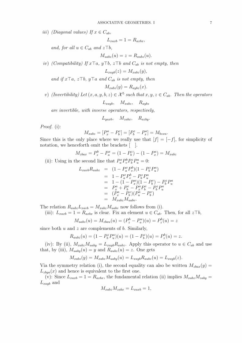
Proposition 1.1.
i) (Symmetry) Mxabz is invariant under permutations of indices by the Klein4-group:
Mxabz = Maxzb = Mbzxa = Mzbax.
ii) (Fundamental Relation) Whenever u, x>a and v, z>b,
RaubzLxavb = MxabzMuabv = LxavbRaubz.
ASSOCIATIVE GEOMETRIES. I 7
iii) (Diagonal values) If x ∈ Cab,
Lxaxb = 1 = Raxbx,
and, for all u ∈ Cab and z>b,Muabz(u) = z = Raubz(u).
iv) (Compatibility) If x>a, y>b, z>b and Cab is not empty, then
Lxayb(z) = Mxabz(y),
and if x>a, z>b, y>a and Cab is not empty, then
Mxabz(y) = Raybz(x).
v) (Invertibility) Let (x, a, y, b, z) ∈ X 5 such that x, y, z ∈ Cab. Then the operators
Lxayb, Mxabz, Raybz
are invertible, with inverse operators, respectively,
Lyaxb, Mzabx, Razby.
Proof. (i):Mxabz = [P a
x − P zb ] = [P z
b − P ax ] = Mbzxa.
Since this is the only place where we really use that [f ] = [−f ], for simplicity ofnotation, we henceforth omit the brackets [ ].
Mzbax = P bz − P x
a = (1− P zb )− (1− P a
x ) = Mxabz
(ii): Using in the second line that P xa P
bvP
zb P
au = 0:
LxavbRaubz = (1− P xa P
bv )(1− P z
b Pau )
= 1− P xa P
bv − P z
b Pau
= 1− (1− P ax )(1− P v
b )− P zb P
au
= P ax + P v
b − P axP
vb − P z
b Pau
= (P ax − P z
b )(P au − P v
b )= MxabzMuabv.
The relation RaubzLxavb = MxabzMuabv now follows from (i).(iii): Lxaxb = 1 = Raxbx is clear. Fix an element u ∈ Cab. Then, for all z>b,
Muabz(u) = Mzbau(u) = (P bz − P u
a )(u) = P bz (u) = z
since both u and z are complements of b. Similarly,
Raubz(u) = (1− P zb P
au )(u) = (1− P z
b )(u) = P bz (u) = z.
(iv): By (ii), MxabzMuaby = LxaybRaubz. Apply this operator to u ∈ Cab and usethat, by (iii), Muaby(u) = y and Raubz(u) = z. One gets
Mxabz(y) = MxabzMuaby(u) = LxaybRaubz(u) = Lxayb(z).
Via the symmetry relation (i), the second equality can also be written Mzbax(y) =Lzbya(x) and hence is equivalent to the first one.
(v): Since Lxaxb = 1 = Raxbx, the fundamental relation (ii) implies MxabzMzaby =Lxayb and
MxabzMzabx = Lxaxb = 1,

8 WOLFGANG BERTRAM AND MICHAEL KINYON
hence Mxabz is invertible with inverse Mzabx. The other relations are proved simi-larly. �
Remark. We will prove in Chapter 2 by different methods that the assumptionCab 6= ∅ in (iv) is unnecessary.
Definition (of the product map Γ). We define a map Γ : D(Γ) → X on thefollowing domain of definition: let
DL := {(x, a, y, b, z) ∈ X 5 | x>a and y>b}DR := {(x, a, y, b, z) ∈ X 5 | y>a and z>b}DM := {(x, a, y, b, z) ∈ X 5 | x>a, z>b and Cab 6= ∅}D(Γ) := DL ∪DR ∪DM ,
and define Γ : D(Γ)→ X by
Γ(x, a, y, b, z) :=
Lxayb(z) if (x, a, y, b, z) ∈ DL
Raybz(x) if (x, a, y, b, z) ∈ DR
Maxbz(y) if (x, a, y, b, z) ∈ DM .
This is well-defined: if (x, a, y, b, z) ∈ DL ∩ DR, then y ∈ Cab, hence Cab is notempty and the preceding proposition implies that
Lxayb(z) = Mxabz(y) = Raybz(x).
Similar remarks apply to the cases (x, a, y, b, z) ∈ DL ∩DM or (x, a, y, b, z) ∈ DR ∩DM . The quintary map Γ explains our terminology and notation: Lxayb is the leftmultiplication operator, acting on the last argument z, and similarly R and Mdenote right and middle multiplication operators. ¿From the definition it followseasily that the symmetry relation
Γ(x, a, y, b, z) = Γ(z, b, y, a, x)
holds for all (x, a, y, b, z) ∈ D(Γ). On the other hand, the relation
Γ(x, a, y, b, z) = Γ(a, x, y, z, b)
holds if (x, a, y, z, b) ∈ DM ; but at present it is somewhat complicated to show thatthis relation is valid on all of D(Γ) (this will follow from the results of Chapter 2).As to the “diagonal values”, for x ∈ Cab we have
Γ(x, a, x, b, z) = z = Γ(z, b, x, a, x) .
If we assume just a>x and b>z, then we can only say in general that
Γ(x, a, x, b, z) = (1− P zb P
ax )(x) = P b
z (x) ⊂ z .
If a, b>x and b>z, then, thanks to the symmetry relation Mxabz = Maxzb,
(1.1) Mxabz(a) = Γ(x, a, a, b, z) = Γ(a, x, a, z, b) = b .
Definition (of the dilation map Πs). Fix s ∈ K. Let
D(Πs) := {(x, a, z) ∈ X 3 | x>a or z>a}

ASSOCIATIVE GEOMETRIES. I 9
and define a ternary map Πs : D(Πs)→ X by
Πs(x, a, z) :=
{δ
(s)xa (z) if x>aδ
(1−s)za (x) if z>a.
As above, this map is well-defined. The symmetry relation
Πs(x, a, y) = Π1−s(y, a, x)
follows easily from the definition. Note that, if s is invertible in K and x>a, then
the dilation operator δ(s)xa is invertible with inverse δ
(s−1)xa .
1.3. Grassmannian torsors and their actions. Recall from §0.2 and AppendixA the definition and elementary properties of torsors.
Theorem 1.2. The Grassmannian geometry (X ; Γ,Πr) defined in the precedingsubsection has the following properties:
i) For a, b ∈ X fixed, Cab with product
(xyz) := Γ(x, a, y, b, z)
is a torsor (which will be denoted by Uab). In particular, for a triple (a, y, b)with y ∈ Cab, Cab is a group with unit y and multiplication xz = Γ(x, a, y, b, z).
ii) The map Γ is symmetric under the permutation (15)(24) (reversal of argu-ments):
Γ(x, a, y, b, z) = Γ(z, b, y, a, x)
In other words, Uab is the opposite torsor of Uba (same set with reversed prod-uct). In particular, the torsor Ua := Uaa is commutative.
iii) The commutative torsor Ua is the underlying additive torsor of an affine space:for any a ∈ X , Ua is an affine space over K, with additive structure given by
x+y z = Γ(x, a, y, a, z),
(sum of x and z with respect to the origin y), and action of scalars given by
sy + (1− s)x = Πs(x, y)
(multiplication of y by s with respect to the origin x).
Proof. (i) Let us show first that Cab is stable under the ternary map (xyz). Letx, y, z ∈ Cab and consider the bijective linear map g := Mxabz. We show thatg(y) ∈ Cab. By equation (1.1), we have the “diagonal values” Mxabz(a) = b andMxabz(b) = a. Thus, if y is complementary to a and b, g(y) is complementary bothto g(a) = b and to g(b) = a, which means that g(y) ∈ Cab.
The associativity follows immediately from the “fundamental relation” (Proposi-tion 1.1(ii)):
(xv(yuz)) = LxavbRaubz(y) = RaubzLxavb(y) = ((xvy)uz),
and the idempotent laws from
(xxy) = Lxaxb(y) = 1(y) = y, (yxx) = Raxbx(y) = 1(y) = y.
Thus Cab is a torsor.(ii) This has already been shown in the preceding section.
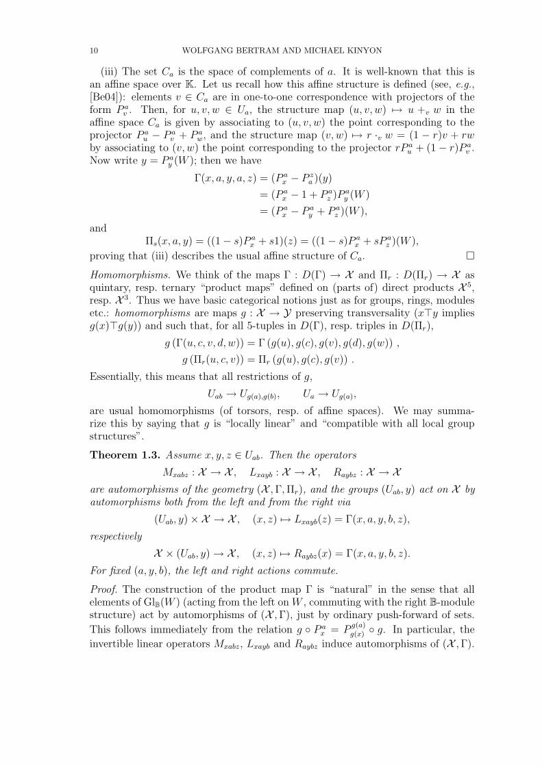
10 WOLFGANG BERTRAM AND MICHAEL KINYON
(iii) The set Ca is the space of complements of a. It is well-known that this isan affine space over K. Let us recall how this affine structure is defined (see, e.g.,[Be04]): elements v ∈ Ca are in one-to-one correspondence with projectors of theform P a
v . Then, for u, v, w ∈ Ua, the structure map (u, v, w) 7→ u +v w in theaffine space Ca is given by associating to (u, v, w) the point corresponding to theprojector P a
u − P av + P a
w, and the structure map (v, w) 7→ r ·v w = (1 − r)v + rwby associating to (v, w) the point corresponding to the projector rP a
u + (1− r)P av .
Now write y = P ay (W ); then we have
Γ(x, a, y, a, z) = (P ax − P z
a )(y)
= (P ax − 1 + P a
z )P ay (W )
= (P ax − P a
y + P az )(W ),
andΠs(x, a, y) = ((1− s)P a
x + s1)(z) = ((1− s)P ax + sP a
z )(W ),
proving that (iii) describes the usual affine structure of Ca. �
Homomorphisms. We think of the maps Γ : D(Γ) → X and Πr : D(Πr) → X asquintary, resp. ternary “product maps” defined on (parts of) direct products X 5,resp. X 3. Thus we have basic categorical notions just as for groups, rings, modulesetc.: homomorphisms are maps g : X → Y preserving transversality (x>y impliesg(x)>g(y)) and such that, for all 5-tuples in D(Γ), resp. triples in D(Πr),
g (Γ(u, c, v, d, w)) = Γ (g(u), g(c), g(v), g(d), g(w)) ,
g (Πr(u, c, v)) = Πr (g(u), g(c), g(v)) .
Essentially, this means that all restrictions of g,
Uab → Ug(a),g(b), Ua → Ug(a),
are usual homomorphisms (of torsors, resp. of affine spaces). We may summa-rize this by saying that g is “locally linear” and “compatible with all local groupstructures”.
Theorem 1.3. Assume x, y, z ∈ Uab. Then the operators
Mxabz : X → X , Lxayb : X → X , Raybz : X → Xare automorphisms of the geometry (X ,Γ,Πr), and the groups (Uab, y) act on X byautomorphisms both from the left and from the right via
(Uab, y)×X → X , (x, z) 7→ Lxayb(z) = Γ(x, a, y, b, z),
respectively
X × (Uab, y)→ X , (x, z) 7→ Raybz(x) = Γ(x, a, y, b, z).
For fixed (a, y, b), the left and right actions commute.
Proof. The construction of the product map Γ is “natural” in the sense that allelements of GlB(W ) (acting from the left on W , commuting with the right B-modulestructure) act by automorphisms of (X ,Γ), just by ordinary push-forward of sets.
This follows immediately from the relation g ◦ P ax = P
g(a)g(x) ◦ g. In particular, the
invertible linear operators Mxabz, Lxayb and Raybz induce automorphisms of (X ,Γ).

ASSOCIATIVE GEOMETRIES. I 11
Now fix y ∈ Uab and consider it as the unit in the group (Uab, y). The claim onthe left action amounts to the identities Lyayb = id (which we already know) and,for all x, x′ ∈ Uab and all z ∈ X ,
Γ(x, a, y, b,Γ(x′, a, y, b, z)) = Γ(Γ(x, a, y, b, x′), a, y, b, z).
First, note that, if z is “sufficiently nice”, i.e., such that the fundamental relation(Proposition 1.1(ii)) applies, then this holds indeed. We will show in Chapter 2that the identity in question holds very generally, and this will prove our claim.Therefore we leave it as a (slighly lengthy) exercise to the interested reader toprove the claim in the present framework. The claims concerning the right actionare proved in the same way, and the fact that both actions commute is preciselythe content of the fundamental relation (Proposition 1.1(ii)) �
Inner automorphisms. We call automorphisms of the geometry defined by the pre-ceding theorem inner automorphisms, and the group generated by them the innerautomorphism group. Note that middle multiplications Mxabz are honest automor-phisms of the geometry (X ,Γ), although they are anti -automorphisms of the torsorUab; this is due to the fact that they exchange a and b. On the other hand, Lxayb
and Raybz are automorphisms of the whole geometry and of Uab.Note also that the action of the groups Uab is of course very far from being regular
on its orbits, except on Uab itself. For instance, a and b are fixed points of theseactions, since Γ(x, a, y, b, b) = b and Γ(x, a, y, b, a) = a.
Finally, the statements of the preceding two theorems amount to certain algebraicidentities for the multiplication map Γ. This will be taken up in Chapter 2, wherewe will not have to worry about domains of definition.
1.4. Affine picture of the torsor Uab. It is useful to have “explicit formulas” forour map Γ. Such formulas can be obtained by introducing “coordinates” on X inthe following way (see [Be04]). First of all, choose a base point (o+, o−) and considerthe pair geometry (X+,X−), where X± is the space of all submodules isomorphicto o± and having a complement isomorphic to o∓. We identify X+ with injectionsx : o+ → W of B right-modules, modulo equivalence under the action of the groupG := Gl(o+) (x ∼= x ◦ g, where g acts on o+ on the left), and X− with B-linearsurjections a : W → o+ (modulo equivalence a ∼= g ◦ a for g ∈ G). Equivalenceclasses are denoted by [x], resp. [a].
Proposition 1.4. The following explicit formulae hold for x, y, z ∈ X+, a, b ∈ X−.
i) if x>a and z>b (middle multiplication), then
(1.2) Γ(
[x], [a], [y], [b], [z])
=[x(ax)−1ay − y + z(bz)−1by
],
ii) if a>x and b>y (left multiplication), then
(1.3) Γ(
[x], [a], [y], [b], [z])
=[x(ax)−1ay(by)−1(bz)− y(by)−1(bz) + z
],
iii) if a>y and b>z (right multiplication), then
(1.4) Γ(
[x], [a], [y], [b], [z])
=[x− y(ay)−1ax+ z(bz)−1za(ay)−1ax
].

12 WOLFGANG BERTRAM AND MICHAEL KINYON
Proof. The right hand side of (1.2) is a well-defined element of X , as is seen bereplacing x by x ◦ g, resp. y by y ◦ g, z by z ◦ g and a by g ◦ a, b by g ◦ b. Notethat [x] and [a] are transversal if and only if ax : o+ → o+ is invertible. Now, theoperator
x(ax)−1a : W → o+ → W
has kernel a and image x and is idempotent, therefore it is P ax . Similarly, we
see that z(bz)−1b is P bz , and hence the right hand side is induced by the operator
P ax − 1 + P b
z = Mxabz. Similarly, we see that the right hand side of (1.3) is inducedby the linear operator
P axP
by − P b
y + 1 = (P ax − 1)P b
y + 1 = 1− P xa P
by = Laxby
and the one of (1.4) by 1− P ay + P b
zPay = 1 + (P b
z − 1)P ay = 1− P z
b Pay = Rzbya. �
As usual in projective geometry, the projective formulas from the preceding resultmay be affinely re-written: if y>b, we may affinize by taking ([y], [b]) as base point(o+, o−): we write W = o− ⊕ o+; then injections x : o+ → W , z : o+ → W that aretransversal to the first factor can be identified with column vectors (by normalizingthe second component to be the identity operator on o+)
x =
(X1
), z =
(Z1
)(columns with X,Z ∈ Hom(o+, o−)). In other terms, x and z are graphs of linearoperators X,Z : o+ → o−. Surjections a : W → o+ that are transversal to thesecond factor correspond to row vectors (A, 1) (row with A ∈ Hom(o−, o+)). Note,however, that the kernel of (A, 1) is determined by the condition Au + v = 0,i.e., v = −Au, and hence a is the graph of −A : o− → o+. Therefore we writea = (−A, 1). The base point y = o+ is the column (0, 1)t, and the base point b = o−
is the row (0, 1). Since ax = (−A, 1)(X, 1)t = 1 − AX, a and x are transversal iff1−AX : o+ → o+ is an invertible operator (in Jordan theoretic language: the pair(X,A) is quasi-invertible, cf. [Lo75]). Using this, any of the three formulas from thepreceding proposition leads to the “affine picture”:
Γ(x, a, y, b, z) =
[(X1
)(1− AX)−1 −
(01
)+
(Z1
)]=
[(−ZAX +X + Z
1
)].
Finally, identifying x with X, y with Y and so on, we may write
Γ(X,A,O+, O−, Z) = X − ZAX + Z .
This formula is interesting in many respects: it is affine in all three variables, andthe product ZAX from the associative pair
(Hom(o+, o−),Hom(o−, o+)
)shows up.
We will give conceptual explanations of these facts later on. Also, it is an easyexercise to check directly that (X,Z) 7→ X − ZAX + Z defines an associativeproduct on Hom(o+, o−) and induces a group structure on the set of elements Xsuch that 1− AX is invertible.

ASSOCIATIVE GEOMETRIES. I 13
Other “rational” formulas. More generally, having fixed (o+, o−), we may write a, bas row-, and x, y, z as column vectors, and then we get the general formula
Γ(X,A, Y,B, Z) =[(X1
)(1− AX)−1(1− AY )−
(Y1
)+
(Z1
)(1−BZ)−1(1−BY )
],
which is (the class of) a vector with second component (“denominator”)
D := (1− AX)−1(1− AY )− 1 + (1−BZ)−1(1−BY ),
and first component (“numerator”)
N := X(1− AX)−1(1− AY )− Y + Z(1−BZ)−1(1−BY ),
so that the affine formula is Γ(X,A, Y,B, Z) = ND−1. Besides the above choice(Y = O+, B = O−), another reasonable choice is just B = O−, leading to
Γ(X,A, Y,O−, Z) = X − (Y − Z)(1− AY )−1(1− AX) .
Similarly, for Y = O+ we get formulas that, in case A = B, correspond to well-known Jordan theoretic formulas for the quasi-inverse. Such formulas show that, ifwe work in finite dimension over a field, Γ is a rational map in the sense of algebraicgeometry, and if we work in a topological setting over topological fields or rings,then Γ will have smoothness properties similar to the ones described in [BeNe05].
Case of a geometry of the first kind. Assume there is a transversal triple, say,(o+, e, o−). We may assume that e is the diagonal in W = o− ⊕ o+. Take, inthe formulas given above, a = 0 = (0, 1), b = ∞ = (1, 0), y = (1, 1)t, ax =(0, 1)(X, 1)t = 1, bz = (1, 0)(Z, 1)t = Z, ay = 1, by = 1, so we get
Γ(X, 0, e,∞, Z) =
[(X1
)−(
11
)+
(Z1
)Z−1
]=
[(XZ−1
)]=
[(XZ
1
)],
and hence the affine picture is the algebra EndB(o+) with its usual product. Takinga =∞, b = 0 gives the opposite of the usual product. Replacing e by y = {(v, Y v) |Y : o+ → o−} (graph of an invertible linear map Y ), we get the affine picture
Γ(X, 0, Y,∞, Z) =
[(XY −1Z
1
)].
1.5. Affinization: the transversal case. If a and b are arbitrary, then in generalthe torsor Uab will be empty. Therefore we look at the pair (Ua, Ub).
Theorem 1.5. For all a, b ∈ X , we have
Γ(Ua, a, Ub, b, Ua) ⊂ Ua, Γ(Ub, a, Ua, b, Ub) ⊂ Ub .
In other words, the maps
Ua × Ub × Ua → Ua; (x, y, z) 7→ (xyz)+ := Lxayb(z) = Γ(x, a, y, b, z) ,
Ub × Ua × Ub → Ub; (x, y, z) 7→ (xyz)− := Raybz(x) = Γ(x, a, y, b, z)

14 WOLFGANG BERTRAM AND MICHAEL KINYON
are well-defined. If, moreover, a>b, then both maps are trilinear, and they form anassociative pair, i.e., they satisfy the para-associative law (cf. Appendix B)
(xy(uvw)±)± = ((xyu)±vw)± = (x(vuy)∓w)±.
Proof. Assume that x>a and y>b. By a direct calculation, we will show thatLxayb(Ua) ⊂ Ua. Let us write Lxayb in matrix form with respect to the decompositionW = a⊕ x. The projectors P x
a and P by can be written
P xa =
(1 00 0
), P b
y =
(α βγ δ
)whith α ∈ End(a), β ∈ Hom(x, a), etc. Thus
Lxayb = 1−(
1 00 0
)(α βγ δ
)=
(1− α −β
0 1
).
Let z ∈ Ua; it can be written as the graph {(Zv, v)| v ∈ x} of a linear operatorZ : x→ a. Since
Lxayb
(Zvv
)=
(1− α −β
0 1
)(Zvv
)=
((1− α)Zv − βv
v
),
Lxayb(z) is the graph of the linear operator (1 − α)Z − β : x → a, and hence isagain transversal to a, so ( )+ is well-defined. By symmetry, it follows that ( )−
is well-defined. Moreover, the calculation shows that z 7→ (xyz)+ is affine (we willsee later that this map is actually affine with respect to all three variables, seeCorollary 2.9).
Now assume that a>b, and write Lxayb in matrix form with respect to the de-composition W = a⊕ b. The projectors P a
x and P by can be written
P ax =
(0 X0 1
), P b
y =
(1 0Y 0
)where X ∈ Hom(b, a) and Y ∈ Hom(a, b). We get
Lxayb = 1−(
1−(
0 X0 1
))(1 0Y 0
)= 1−
(1−XY 0
0 0
)=
(XY 0
0 1
)and, writing z ∈ Ua as a graph {(Zv, v)|v ∈ b}, we get
Lxayb
(Zvv
)=
(XY 0
0 1
)(Zvv
)=
(XY Zvv
),
hence Lxayb(z) is the graph of XY Z : b → a. Thus, with V + = Ua∼= Hom(b, a),
V − = Ub∼= Hom(a, b), the first ternary map is given by
V + × V − × V + → V +, (X, Y, Z) 7→ XY Z.
Similarly, one shows that the second ternary map is given by
V − × V + × V − → V −, (X, Y, Z) 7→ ZY X.
This pair of maps is the prototype of an associative pair (see Appendix B). �

ASSOCIATIVE GEOMETRIES. I 15
At this stage, the appearance of the trilinear expression ZY X, resp. ZAX, bothin the affine pictures of the map from the preceding theorem and in the precedingsection, related by the identity
(1.5) X − (X − ZAX + Z) + Z = ZAX,
looks like a pure coincidence. A conceptual explanation will be given in Chapter 3(Lemma 3.2).
2. Grassmannian semitorsors
In this chapter we extend the definition of the product map Γ onto all of X 5, andwe show that the most important algebraic identities extend also. We use notationand general notions explained in the first section of the preceding chapter.
2.1. Composition of relations. Recall that, if A,B,C, . . . are any sets, we cancompose relations : for subsets x ⊂ A×B, y ⊂ B × C,
y ◦ x := yx := {(u,w) ∈ A× C | ∃v ∈ B : (u, v) ∈ x, (v, w) ∈ y} .Composition is associative: both (z ◦ y) ◦ x and z ◦ (y ◦ x) are equal to
(2.1) z ◦ y ◦ x = {(u,w) ∈ A×D | ∃(v1, v2) ∈ y : (u, v1) ∈ x, (v2, w) ∈ z} .If x and y are graphs of maps X, resp. Y (v = Xu, w = Y v) then y ◦x is the graphof Y X (w = Y v = Y Xu). The reverse relation of x is
x−1 := {(w, v) ∈ B × A | (v, w) ∈ x}.We have (yx)−1 = x−1y−1, and if x is the graph of a bijective map, then x−1 is thegraph of its inverse map. For x, y, z ⊂ A × B, we get another relation between Aand B by zy−1x. Obviously, this ternary composition satisfies the para-associativelaw, and hence relations between A and B form a semitorsor. Letting W := A×B,we have the explicit formula
zy−1x =
{ω = (α′, β′) ∈ W
∣∣∣ ∃η = (α′′, β′′) ∈ y :(α′, β′′) ∈ x, (α′′, β′) ∈ z
}=
{ω ∈ W
∣∣∣ ∃α′, α′′ ∈ A,∃β′, β′′ ∈ B, ∃η ∈ y,∃ξ ∈ x,∃ζ ∈ z :ω = (α′, β′), η = (α′′, β′′), ξ = (α′, β′′), ζ = (α′′, β′)
}2.2. Composition of linear relations. Now assume that A,B,C, . . . are linearspaces over B (i.e., right modules) and that all relations are linear relations (i.e.,submodules of A ⊕ B, etc.). Then zy−1x is again a linear relation. Identifying Awith the first and B with the second factor in W := A ⊕ B, the description ofzy−1x given above can be rewritten, by introducing the new variables α := α′−α′′,β := β′ − β′′,
zy−1x =
{ω ∈ W
∣∣∣ ∃α′, α′′ ∈ a,∃β′, β′′ ∈ b,∃η ∈ y,∃ξ ∈ x,∃ζ ∈ z :ω = α′ + β′, η = α′′ + β′′, ξ = α′ + β′′, ζ = α′′ + β′
}=
{ω ∈ W
∣∣∣ ∃α′, α ∈ a,∃β′, β ∈ b,∃η ∈ y,∃ξ ∈ x,∃ζ ∈ z :ω = α′ + β′, η = ω − α− β, ξ = ω − β, ζ = ω − α
}.
In order to stress that the product xy−1z depends also on A and B, we will hence-forth use lowercase letters a and b and write W = a⊕ b.
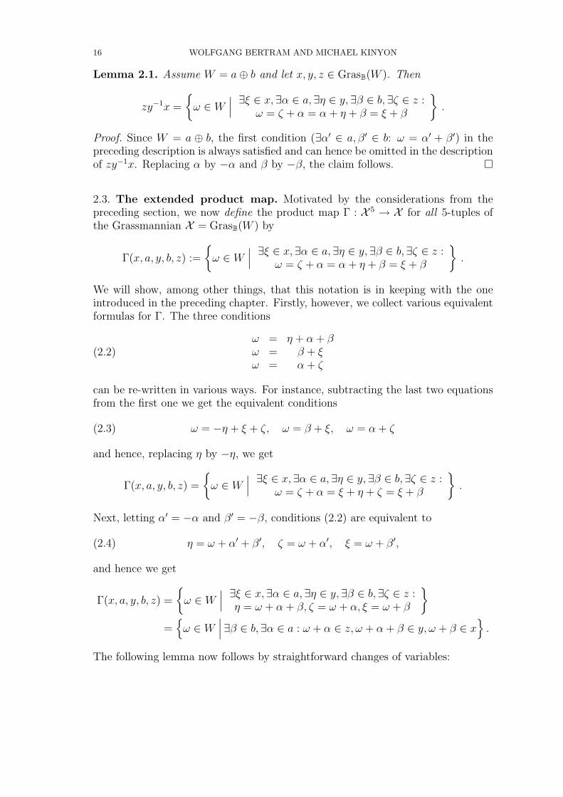
16 WOLFGANG BERTRAM AND MICHAEL KINYON
Lemma 2.1. Assume W = a⊕ b and let x, y, z ∈ GrasB(W ). Then
zy−1x =
{ω ∈ W
∣∣∣ ∃ξ ∈ x,∃α ∈ a,∃η ∈ y,∃β ∈ b, ∃ζ ∈ z :ω = ζ + α = α + η + β = ξ + β
}.
Proof. Since W = a ⊕ b, the first condition (∃α′ ∈ a, β′ ∈ b: ω = α′ + β′) in thepreceding description is always satisfied and can hence be omitted in the descriptionof zy−1x. Replacing α by −α and β by −β, the claim follows. �
2.3. The extended product map. Motivated by the considerations from thepreceding section, we now define the product map Γ : X 5 → X for all 5-tuples ofthe Grassmannian X = GrasB(W ) by
Γ(x, a, y, b, z) :=
{ω ∈ W
∣∣∣ ∃ξ ∈ x,∃α ∈ a,∃η ∈ y,∃β ∈ b, ∃ζ ∈ z :ω = ζ + α = α + η + β = ξ + β
}.
We will show, among other things, that this notation is in keeping with the oneintroduced in the preceding chapter. Firstly, however, we collect various equivalentformulas for Γ. The three conditions
(2.2)ω = η + α + βω = β + ξω = α + ζ
can be re-written in various ways. For instance, subtracting the last two equationsfrom the first one we get the equivalent conditions
(2.3) ω = −η + ξ + ζ, ω = β + ξ, ω = α + ζ
and hence, replacing η by −η, we get
Γ(x, a, y, b, z) =
{ω ∈ W
∣∣∣ ∃ξ ∈ x,∃α ∈ a,∃η ∈ y,∃β ∈ b, ∃ζ ∈ z :ω = ζ + α = ξ + η + ζ = ξ + β
}.
Next, letting α′ = −α and β′ = −β, conditions (2.2) are equivalent to
(2.4) η = ω + α′ + β′, ζ = ω + α′, ξ = ω + β′,
and hence we get
Γ(x, a, y, b, z) =
{ω ∈ W
∣∣∣ ∃ξ ∈ x,∃α ∈ a,∃η ∈ y,∃β ∈ b,∃ζ ∈ z :η = ω + α + β, ζ = ω + α, ξ = ω + β
}={ω ∈ W
∣∣∣ ∃β ∈ b, ∃α ∈ a : ω + α ∈ z, ω + α + β ∈ y, ω + β ∈ x}.
The following lemma now follows by straightforward changes of variables:

ASSOCIATIVE GEOMETRIES. I 17
Lemma 2.2. For all x, a, y, b, z ∈ X ,
Γ(x, a, y, b, z) ={ω ∈ W
∣∣∣ ∃ξ ∈ x,∃ζ ∈ z : ζ + ω ∈ a, ζ + ω + ξ ∈ y, ω + ξ ∈ b}
={ω ∈ W
∣∣∣ ∃ξ ∈ x,∃α ∈ a : ω − α ∈ z, ξ − α ∈ y, ω − ξ ∈ b}
={ω ∈ W
∣∣∣ ∃β ∈ b, ∃ζ ∈ z : ζ − ω ∈ a, ζ − β ∈ y, ω − β ∈ x}
={ω ∈ W
∣∣∣ ∃η ∈ y,∃β ∈ b : ω − η − β ∈ a, β + η ∈ z, ω − β ∈ x}
={ω ∈ W
∣∣∣ ∃η ∈ y,∃ζ ∈ z : ω + ζ ∈ a, ζ + η ∈ b, ω + ζ + η ∈ x}
We refer to the descriptions of the lemma as the “(x, z)-”, “(x, a)-description”,and so on. The (a, b)-description is particularly useful for the proof of the theorembelow. One may note that the only pairs of variables that cannot be used for sucha description are (a, z) and (x, b), and that the signs in the terms appearing inthese descriptions can be chosen positive if the pair is “homogeneous” (a subpairof (x, y, z) or of (a, b)), whereas for “mixed” pairs we cannot get rid of signs.
Theorem 2.3. The map Γ : X 5 → X extends the product map defined in thepreceding chapter, and has the following properties:
(1 ) It is symmetric under the Klein 4-group:
Γ(x, a, y, b, z) = Γ(z, b, y, a, x) ,(a)
Γ(x, a, y, b, z) = Γ(a, x, y, z, b) .(b)
(2 ) For any pair (a, b) ∈ X 2, the product (xyz) := Γ(x, a, y, b, z) on X 3 satisfies theproperties of a semitorsor, that is,
Γ(x, a, u, b,Γ(y, a, v, b, z)
)= Γ
(x, a,Γ(v, a, y, b, u), b, z
)= Γ
(Γ(x, a, u, b, y), a, v, b, z
).
We will write Xab for X equipped with this semitorsor structure. Then the semi-torsor Xba is the opposite semitorsor of Xab; in particular, Xaa is a commutativesemitorsor, for any a.
Proof. (1) The symmetry relation (a) is obvious from the definition of Γ. Exchang-ing x and a amounts in the (x, a)-description to exchanging simultaneously z andb, hence the symmetry relation (b) follows.
For (2), we use the (a, b)-description: on the one hand,
Γ(x, a, u, b,Γ(y, a, v, b, z)
)=
=
{ω ∈ W
∣∣∣ ∃α ∈ a,∃β ∈ b :ω + α ∈ Γ(y, a, v, b, z), ω + α + β ∈ u, ω + β ∈ x
}
=
ω ∈ W ∣∣∣ ∃α ∈ a,∃β ∈ b,∃α′ ∈ a,∃β′ ∈ b :ω + α + β ∈ u, ω + β ∈ x, ω + α + α′ ∈ z,
ω + α + α′ + β′ ∈ v, ω + α + β′ ∈ y
On the other hand,

18 WOLFGANG BERTRAM AND MICHAEL KINYON
Γ(x, a,Γ(u, b, y, a, v), b, z
)=
=
{ω ∈ W
∣∣∣ ∃α′′ ∈ a,∃β′′ ∈ b :ω + α′′ ∈ z, ω + α′′ + β′′ ∈ Γ(u, b, y, a, v), ω + β′′ ∈ x
}
=
ω ∈ W ∣∣∣ ∃α′′ ∈ a, ∃β′′ ∈ b, ∃α′′′ ∈ a,∃β′′′ ∈ b :ω + α′′ ∈ z, ω + β′′ ∈ x, ω + α′′ + β′′ + α′′′ ∈ u,
ω + α′′ + β′′ + β′′′ ∈ v, ω + α′′ + β′′ + α′′′ + β′′′ ∈ y
Via the change of variables α′′ = α + α′, α′′′ = α′, β′′ = β, β′′′ = β, we see thatthese two subspaces of W are the same. The remaining equality is equivalent tothe one just proved via the symmetry relation (a).
Next, we show that the new map Γ coincides with the old one on D(Γ). Let usassume that (x, a, y, b, z) ∈ DL, so x>a and y>b. We use the (y, b)-description andlet ζ := η + β, whence η = P b
y ζ and β = P yb ζ. We get
Γ(x, a, y, b, z) ={ω ∈ W
∣∣∣∃η ∈ y,∃β ∈ b : ω − η − β ∈ a, β + η ∈ z, ω − β ∈ x}
={ω ∈ W
∣∣∣∃ζ ∈ z : ω − P yb (ζ) ∈ x, ω − ζ ∈ a
}={ω ∈ W
∣∣∣∃ζ ∈ z : P ax (ω − ζ) = 0, P a
x (ω − P yb (ζ)) = ω − P y
b (ζ)}
={ω ∈ W
∣∣∣∃ζ ∈ z : P ax ζ = P a
xω, ω = P yb ζ + P a
xω − P axP
yb ζ}
={ω ∈ W
∣∣∣∃ζ ∈ z : ω = (P yb + P a
x − P axP
yb )ζ}
and a straightforward calculation shows that
P yb + P a
x − P axP
yb = 1− P x
a Pby = Lxayb
so that Γ(x, a, y, b, z) = Lxayb(z). This proves that the old and new definitions ofΓ coincide on DL, and hence also on DR by the symmetry relation. Now we showthat the new map Γ coincides with the old one on DM : assume a>x and b>z anduse the (x, z)-description; let η := ζ−ω+ ξ and observe that P a
x η = P ax ξ = ξ (since
ζ − ω ∈ a), and similarly P bz η = ζ, whence ω = ζ − η + ξ = (P b
z − 1 + P ax )η, and
thus
Γ(x, a, y, b, z) ={ω ∈ W
∣∣∣ ∃ξ ∈ x,∃ζ ∈ z : ζ − ω ∈ a, ζ − ω + ξ ∈ y, ω − ξ ∈ b}
={ω ∈ W
∣∣∣ ∃η ∈ y : ω = (P bz − 1 + P a
x )η},
that is, ω = −Mxabzη, and hence Γ(x, a, y, b, z) = Mxabz(y). �
2.4. Diagonal values. We call diagonal values the values taken by Γ on the subsetof X 5 where at least two of the five variables x, a, y, b, z take the same value. Thereare two different kinds of behavior on such diagonals: for the diagonal a = b (or,equivalently, x = z), we still have a rich algebraic theory which is equivalent to theJordan part of our associative products; this topic is left for subsequent work (cf.Chapter 4). The three remaining diagonals (x = y, resp. a = z, resp. b = z) havean entirely different behavior: the algebraic operation Γ restricts in these cases tolattice theoretic operations, that is, can be expressed by intersections and sums of

ASSOCIATIVE GEOMETRIES. I 19
subspaces. We will use the lattice theoretic notation x∧y = x∩y and x∨y = x+y.It is remarkable that two important aspects of projective geometry (the latticetheoretic and the Jordan theoretic) arise as a sort of “contraction” of the full mapΓ, or, put differently, that they have a common “deformation”, given by Γ.
Theorem 2.4. The map Γ : X 5 → X takes the following diagonal values:
(1 ) values on the “diagonal x = y”: for all (x, a, b, z) ∈ X 4,
Γ(x, a, x, b, z) = (z ∨ (x ∧ a)) ∧ (b ∨ x).
In particular, we get the following “subdiagonal values”: for all x, a, y, b, z,(i) subdiagonal x = y = z: Γ(x, a, x, b, x) = x (law (xxx) = x in Xab),
(ii) subdiagonal x = y = a: Γ(x, x, x, b, z) = (z ∨ x) ∧ (b ∨ x)(iii) subdiagonal x = y = a and b = z: Γ(x, x, x, z, z) = z ∨ x(iv) subdiagonal x = y = b: Γ(x, a, x, x, z) = (z ∨ (x ∧ a)) ∧ x.(v) subdiagonal x = y = b and a = z: Γ(x, a, x, x, a) = a ∧ x
(vi) subdiagonal x = y, a = z: Γ(x, a, x, b, a) = a ∧ (b ∨ x)(vii) subdiagonal x = y, a = b: Γ(x, a, x, a, z) = (z ∨ (x ∧ a)) ∧ (x ∨ a)
(viii) subdiagonal x = y, z = b: Γ(x, a, x, z, z) = z ∨ (x ∧ a)(2 ) diagonal a = z: for all (x, a, y, b) ∈ X 4,
Γ(x, a, y, b, a) = a ∧ (b ∨ (x ∧ (y ∨ a)))
In particular, on the subdiagonal x = z = b, we have, for all x, a, y ∈ X ,
Γ(x, a, y, x, a) = a ∧ x.(3 ) diagonal b = z: for all (x, a, y, b) ∈ X 4,
Γ(x, a, y, b, b) = b ∨ (a ∧ (x ∨ (y ∧ b)))In particular, on the subdiagonal b = z, x = a, we have, for all a, y, b ∈ X ,
Γ(a, a, y, b, b) = b ∨ a,and on a = b = az: for all x, a, y, Γ(x, a, y, a, a) = a.
Proof. In the following proof, in order to avoid unnecessary repetitions, it is alwaysunderstood that α ∈ a, ξ ∈ x, β ∈ b, η ∈ y, ζ ∈ z. In all three items, thedetermination of the “subdiagonal values” is a straightforward consequence, usingthe absorption laws u ∨ (u ∧ v) = u, u ∧ (u ∨ v) = u.
Now we prove (1) (diagonal x = y). Let ω ∈ Γ(x, a, x, b, z), then ω = ξ+β, henceω ∈ (x ∨ b), and ω = η + ξ + ζ with v := ω − ζ = η + ξ ∈ x (since x = y). On theother hand, v = ω − ζ = α ∈ a, whence ω = v + ζ with v ∈ (x ∧ a), proving oneinclusion.
Conversely, let ω ∈ (z∨(x∧a))∧(b∨x). Then ω = β+ξ = α+ζ with α ∈ (x∧a).Let η := ξ − α. Then η ∈ x, and ω = ξ + β = η + α + β, hence ω ∈ Γ(x, a, x, b, z).
Next we prove (2) (diagonal a = z). Let ω ∈ Γ(x, a, y, b, a), then ω = ζ + α withζ, α ∈ z = a, whence ω ∈ a. Moreover, ω = ξ + β = η + α + β, with η + α = ξ ∈ xand η + α ∈ y ∨ a, whence ω ∈ b ∨ (x ∧ (y ∨ a)).
Conversely, let ω ∈ a ∧ (b ∨ (x ∧ (y ∨ a))). Then ω ∈ b ∨ (x ∧ (y ∨ a)), that is,ω = β + (η + α) with ξ := η + α ∈ x. Letting ζ := ω − α ∈ a (here we use thatω ∈ a), we have ω = ζ + α, proving that ω ∈ Γ(x, a, y, b, a).

20 WOLFGANG BERTRAM AND MICHAEL KINYON
The proof for (3) (diagonal z = b) is “dual” to the preceding one and will be leftto the reader. �
Remark. By arguments of the same kind as above, one can show that the diagonalvalue for x = y (part (1)) admits also another, kind of “dual”, expression:
(2.5) Γ(x, a, x, b, z) = (z ∧ (x ∨ b)) ∨ (a ∧ x).
The equality of these two expressions is equivalent to the modular law
(2.6) Γ(x, a, x, x, z) = (z ∧ x) ∨ (a ∧ x) = ((z ∧ x) ∨ a) ∧ x.It is known [PR09] that any (finitely based) variety of lattices can be axiomatized
by a single quaternary operation q(·, ·, ·, ·) given in terms of the lattice operationsby q(x, b, z, a) = (z ∧ (x ∨ b)) ∨ (a ∧ x). That is, one may start with a quarternaryoperation q satisfying certain identities (which we omit), define x∨ y = q(y, x, x, y)and x ∧ y = q(y, y, x, x), and the resulting structure will be a lattice. From thepreceding paragraph, we see that in our setting, q(x, b, z, a) = Γ(x, a, x, b, z). Thusthe quaternary approach to lattices emerges from the present theory in a completelynatural way.
Corollary 2.5. (1 ) If b ∨ x = W and a ∧ x = 0, then Γ(x, a, x, b, z) = z.(2 ) If a ∨ y = W and b ∨ x = W , then Γ(x, a, y, b, a) = a.(3 ) If x ∧ a = 0 and y ∧ b = 0, then Γ(x, a, y, b, b) = b.
Proof. Straightforward consequences of the theorem, again using the absorptionlaws. �
2.5. Structural transformations and self-distributivity. Homomorphisms be-tween sets with quintary product maps Γ, Γ′ are defined in the usual way, and mayserve to define the category of Grassmannian geometries with their product mapsΓ. We call this the “usual” category. There is another and often more useful wayto turn them into a category which we call “structural”:
Definition. Let W,W ′ be two right B-modules and (X ,Γ), (X ′,Γ′) their Grass-mannian geometries. A structural or adjoint pair of transformations between Xand X ′ is a pair of maps f : X → X ′, g : X ′ → X such that, for all x, a, y, b, z ∈ X ,x′, a′, y′, b′, z′ ∈ X ′,
f(Γ(x, g(a′), y, g(b′), z)
)= Γ′(f(x), a′, f(y), b′, f(z)),
g(Γ′(x′, f(a), y′, f(b), z′)
)= Γ(g(x′), a, g(y′), b, g(z′)) .
In other words, for fixed a, b, resp. a′, b′, the restrictions
f : Xg(a′),g(b′) → X ′a′,b′ , g : X ′f(a),f(b) → Xa,b
are homomorphisms of semitorsors. We will sometimes write (f, f t) for a structuralpair (although g need not be uniquely determined by f).
It is easily checked that the composition of structural pairs gives again a struc-tural pair, and Grassmannian geometries with structural pairs as morphisms forma category. Isomorphisms, and, in particular, the automorphism group of (X ,Γ),are essentially the same in the usual and in the structural categories, but the en-domorphism semigroups may be very different. Roughly speaking, Grassmannian
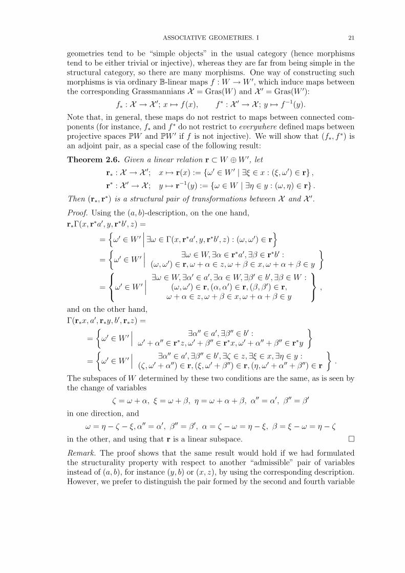
ASSOCIATIVE GEOMETRIES. I 21
geometries tend to be “simple objects” in the usual category (hence morphismstend to be either trivial or injective), whereas they are far from being simple in thestructural category, so there are many morphisms. One way of constructing suchmorphisms is via ordinary B-linear maps f : W → W ′, which induce maps betweenthe corresponding Grassmannians X = Gras(W ) and X ′ = Gras(W ′):
f∗ : X → X ′; x 7→ f(x), f ∗ : X ′ → X ; y 7→ f−1(y).
Note that, in general, these maps do not restrict to maps between connected com-ponents (for instance, f∗ and f ∗ do not restrict to everywhere defined maps betweenprojective spaces PW and PW ′ if f is not injective). We will show that (f∗, f
∗) isan adjoint pair, as a special case of the following result:
Theorem 2.6. Given a linear relation r ⊂ W ⊕W ′, let
r∗ : X → X ′; x 7→ r(x) := {ω′ ∈ W ′ | ∃ξ ∈ x : (ξ, ω′) ∈ r} ,r∗ : X ′ → X ; y 7→ r−1(y) := {ω ∈ W | ∃η ∈ y : (ω, η) ∈ r} .
Then (r∗, r∗) is a structural pair of transformations between X and X ′.
Proof. Using the (a, b)-description, on the one hand,
r∗Γ(x, r∗a′, y, r∗b′, z) =
={ω′ ∈ W ′
∣∣∣∃ω ∈ Γ(x, r∗a′, y, r∗b′, z) : (ω, ω′) ∈ r}
=
{ω′ ∈ W ′
∣∣∣ ∃ω ∈ W,∃α ∈ r∗a′,∃β ∈ r∗b′ :(ω, ω′) ∈ r, ω + α ∈ z, ω + β ∈ x, ω + α + β ∈ y
}
=
ω′ ∈ W ′∣∣∣ ∃ω ∈ W,∃α′ ∈ a′,∃α ∈ W,∃β′ ∈ b′,∃β ∈ W :
(ω, ω′) ∈ r, (α, α′) ∈ r, (β, β′) ∈ r,ω + α ∈ z, ω + β ∈ x, ω + α + β ∈ y
,
and on the other hand,
Γ(r∗x, a′, r∗y, b
′, r∗z) =
=
{ω′ ∈ W ′
∣∣∣ ∃α′′ ∈ a′, ∃β′′ ∈ b′ :ω′ + α′′ ∈ r∗z, ω′ + β′′ ∈ r∗x, ω′ + α′′ + β′′ ∈ r∗y
}=
{ω′ ∈ W ′
∣∣∣ ∃α′′ ∈ a′,∃β′′ ∈ b′,∃ζ ∈ z, ∃ξ ∈ x, ∃η ∈ y :(ζ, ω′ + α′′) ∈ r, (ξ, ω′ + β′′) ∈ r, (η, ω′ + α′′ + β′′) ∈ r
}.
The subspaces of W determined by these two conditions are the same, as is seen bythe change of variables
ζ = ω + α, ξ = ω + β, η = ω + α + β, α′′ = α′, β′′ = β′
in one direction, and
ω = η − ζ − ξ, α′′ = α′, β′′ = β′, α = ζ − ω = η − ξ, β = ξ − ω = η − ζin the other, and using that r is a linear subspace. �
Remark. The proof shows that the same result would hold if we had formulatedthe structurality property with respect to another “admissible” pair of variablesinstead of (a, b), for instance (y, b) or (x, z), by using the corresponding description.However, we prefer to distinguish the pair formed by the second and fourth variable

22 WOLFGANG BERTRAM AND MICHAEL KINYON
in order to have the interpretation of structural transformations in terms of torsorhomomorphisms, for fixed (a, b).
Remark. The construction from the theorem is functorial. In particular, the semi-group of linear relations on W ×W (to be more precise: a quotient with respect toscalars) acts by structural pairs on X .
Theorem 2.7. We define operators of left-, middle- and right multiplication on Xby
Lxayb(z) := Raybz(x) := Mxabz(y) := Γ(x, a, y, b, z).
Then, for all x, a, y, b, z ∈ X , the pairs
(Lxayb, Lyaxb), (Mxabz,Mzabx), (Raybz, Razby)
are structural transformations of the Grassmannian geometry X .
Proof. Let lx,a,y,b ⊂ W ⊕W be the linear relation defined by
lx,a,y,b := {(ζ, ω) ∈ W ⊕W | ∃ξ ∈ x : ω + ζ ∈ a, ω + ζ + ξ ∈ y, ω + ξ ∈ b}.Then it follows immediately by using the (x, z)-description that
(lx,a,y,b)∗(z) = {ω ∈ W | ∃ζ ∈ z : (ζ, ω) ∈ lx,a,y,b} = Γ(x, a, y, b, z) = Lxayb(z).
On the other hand,
(lx,a,y,b)∗(z) = {ω ∈ W | ∃ζ ∈ z : (ω, ζ) ∈ lx,a,y,b}
={ω ∈ W
∣∣∣ ∃ζ ∈ z, ∃ξ ∈ x : ω + ζ ∈ a, ω + ζ + ξ ∈ y, ζ + ξ ∈ b}
= Γ(y, a, x, b, z) = Lyaxb(z) ,
where the third equality follows by using the (y, z)-description with permuted vari-ables. This proves that (Lxayb, Lyaxb) is a structural pair; the claim for right multipli-cations is just an equivalent version of this, and the claim for middle multiplicationsis proved in the same way as above. �
Remark. We have proved that, in terms of inverses of linear relations,
(2.7) (lx,a,y,b)−1 = ly,a,x,b.
If x>a and y>b, then lxaby is the graph of the linear operator Lxayb ∈ End(W ); forx, y ∈ Uab, this operator is invertible and the preceding formula holds in the senseof an operator equation.
Corollary 2.8. The multiplication map satisfies the following “self-distributivity”identities:
Γ(x, a,Γ
(u,Γ(a, z, c, x, b), v,Γ(a, z, d, x, b), w
), b, z
)=
Γ(
Γ(x, a, u, b, z), c,Γ(x, a, v, b, z), d,Γ(x, a, w, b, z))
Γ(x, a, y, b,Γ
(u,Γ(y, a, x, b, c), v,Γ(y, a, x, b, d), w
))=
Γ(
Γ(x, a, y, b, u), c,Γ(x, a, y, b, v), d,Γ(x, a, y, b, w))
ASSOCIATIVE GEOMETRIES. I 23
Proof. The first identity follows by applying the adjoint pair (f, f t) = (Mxabz,Mzabx)to Γ(u, c, v, d, w) (and using the symmetry property), and similarly the second byusing the pair (f, f t) = (Lxayb, Lyaxb). �
Corollary 2.9. For all a, b ∈ X , the maps ( )+ : Ua × Ub × Ua → Ua and( )− : Ub × Ua × Ub → Ub defined in Theorem 1.5 are tri-affine (i.e., affine in allthree variables) and satisfy the para-associative law
(xy(uvw)±)± = ((xyu)±vw)± = (x(vuy)∓w)±.
Proof. Let us show that Mxabz induces an affine map Ub → Ua, y 7→ (xyz)+, forfixed x, z ∈ Ua. We know already that this map is well-defined (Theorem 1.5).Since (f, g) = (Mxabz,Mzabx) is structural, the map f : Ug(a) → Ua is affine, where(according to Corollary 2.5, (1)),
g(a) = Mzabx(a) = Γ(z, a, a, b, x) = Γ(a, z, a, x, b) = b.
By the same kind of argument, using Corollary 2.5, (2) and (3), wee see that theother partial maps are affine. The corresponding statements for ( )− follow bysymmetry, and the para-associative law follows by restriction of the para-associativelaw in the semitorsor Xab. �
Remark. For a = b, we get the additive torsor Ua, and if Uab 6= ∅, then we get a sortof “triaffine extension” of the torsor Uab. If a>b, then we have base points a in Ub
and b in Ua, and obtain a trilinear product (Theorem 1.5).
2.6. The extended dilation map. Next we (re-)define, for r ∈ K, the dilationmap Πr : X × X × X → X by the following equivalent expressions
Πr(x, a, z) :={ω ∈ W
∣∣∣∃α ∈ a,∃ζ ∈ z,∃ξ ∈ x : ω − rα = ξ = ζ − α}
={ω ∈ W
∣∣∣ ∃α ∈ a,∃ζ ∈ z,∃ξ ∈ x : ω + (1− r)α = ζ = α + ξ}
={ω ∈ W
∣∣∣ ∃α ∈ a,∃ζ ∈ z,∃ξ ∈ x : ω = (1− r)ξ + rζ, ζ − ξ = α}
We refer to the last expression as the “(x, z)-description”, and we define partialmaps X → X by
λrxa(z) := ρr
az(x) := µrxz(a) := Πr(x, a, z)
(where λ reminds us of “left”, ρ “right” and µ “middle”).
Theorem 2.10. The map Πr : X 3 → X extends the ternary map defined in thepreceding chapter (and denoted by the same symbol there), and it has the followingproperties:
(1 ) Symmetry: µrxz = µ1−r
zx , that is, λrxa = ρ1−r
ax or
Πr(x, a, z) = Π1−r(z, a, x).
(2 ) Multiplicativity: if x>a and r, s ∈ K,
Πr(x, a,Πs(x, a, y)) = Πrs(x, a, y),
(3 ) Diagonal values:
Πr(x, a, x) = x, Π0(x, a, z) = Π1(z, a, x) = x ∧ (z ∨ a) = Γ(a, x, x, a, z).
24 WOLFGANG BERTRAM AND MICHAEL KINYON
(4 ) Structurality: if r(1− r) ∈ K×, then, for all x, a, z ∈ X , the pairs
(λrxa, λ
rax), (µr
xz, µrzx)
are structural transformations of (X ,Γ).
Proof. The symmetry relation (1) follows directly from the (x, z)-description.Next we show that Πr coincides with the dilation map from the preceding chapter.
Assume first that x>a. We show that Πr(x, a, z) = (rP xa + P a
x )(z):
(rP xa + P a
x )(z) ={e ∈ W
∣∣∣ ∃ζ ∈ z : e = rP xa (ζ) + P a
x (ζ)}
={e ∈ W
∣∣∣ ∃α ∈ a,∃ζ ∈ z,∃ξ ∈ x : e− rα = ζ − α = ξ}
= Πr(x, a, z)
writing ζ = P xa (ζ) + P a
x (ζ) = α + ξ. For z>a, the claim follows now from thesymmetry relation (1).
(3) With ω = (1− r)ξ + rζ, it follows for x = z that Πr(x, a, x) ⊂ x. Conversely,we get x ⊂ Πr(x, a, x) by letting α = 0 and ζ = ξ, given ξ ∈ x. The other relationsare proved similarly.
(2) Under the assumption x>a, the claim amounts to the operator identity
(rP xa + P a
x )(sP xa + P a
x ) = (rsP xa + P a
x )
which is easily checked.(4) Fix x, a ∈ X , r ∈ K and define the linear subspace r ⊂ W ⊕W by
r := rxa :={
(ζ, ω) ∈ W ⊕W | ∃α ∈ a,∃ξ ∈ x : ω = ζ − (1− r)α, ζ − α = x}
Then
r∗(z) = {ω ∈ W | ∃ζ ∈ z : (ζ, ω) ∈ r} = Πr(x, a, z).
On the other hand, by a straightforward change of variables (which is bijective sincer is assumed to be invertible), one checks that
r∗(z) = {ω ∈ W | ∃ζ ∈ z : (ω, ζ) ∈ r} = Πr(a, x, z).
Hence (λrxa, λ
rax) = (r∗, r
∗) is structural. The calculation for the middle multiplica-tions is similar. �
Remarks. 1. If r is invertible, then Πr(a, x, z) = Πr−1(x, a, z). Combining with(1), we see that Π has the same behaviour under permutations as for the classicalcross-ratio.
2. If x>a and r ∈ K an arbitrary scalar, we still have structurality in (4). Thesituation is less clear if x, a, r are all arbitrary.
3. One can define structurality with respect to Πr in the same way as for Γ, byconditions of the form
f(Πr(x, g(a′), z
)= Π′r(f(x), a′, f(z)), g
(Π′r(x
′, f(a), z′)
= Πr(g(x′), a, g(z′)).
Then partial maps of Γ are structural for Πr, and partial maps of Πs are structuralfor Πr (this property has been used in [Be02] to characterize generalized projectivegeometries). The proofs are similar to the ones given above.

ASSOCIATIVE GEOMETRIES. I 25
3. Associative geometries
In this chapter we give an axiomatic definition of associative geometry, and weshow that, at a base point, the corresponding “tangent object” is an associativepair. Conversely, given an associative pair, one can reconstruct an associative ge-ometry. The question whether these constructions can be refined to give a suitableequivalence of categories will be left for future work.
3.1. Axiomatics.
Definition. An associative geometry over a commutative unital ring K is given bya set X which carries the following structures: X is a complete lattice (with joindenoted by x ∨ y and meet denoted by x ∧ y), and maps (where s ∈ K)
Γ : X 5 → X , Πs : X 3 → X ,such that the following holds. We use the notation
Lxaby(z) := Mxabz(y) := Raybz(x) := Γ(x, a, y, b, z)
for the partial maps of Γ, and call x and y transversal, denoted by x>y, if x∧y = 0and x ∨ y = 1, and we let
Ca := a> := {x ∈ X | x>a}, Cab := Ca ∩ Cb
for sets of elements transversal to a, resp. to a and b.
( 1) The semitorsor property: for all x, y, z, u, v, a, b ∈ X :
Γ(Γ(x, a, y, b, z), a, u, b, v) = Γ(x, a,Γ(u, a, z, b, y), b, v) = Γ(x, a, y, b,Γ(z, a, u, b, v)).
In other words, for fixed a, b, the product (xyz) := Γ(x, a, y, b, z) turns X intoa semitorsor, which will be denoted by Xab.
( 2) Invariance of Γ under the Klein 4-group in (x, a, b, z): for all x, a, y, b, z ∈ X ,( i) Γ(x, a, y, b, z) = Γ(z, b, y, a, x)
( ii) Γ(x, a, y, b, z) = Γ(a, x, y, z, b)In particular, Xba is the opposite semitorsor of Xab.
( 3) Structurality of partial maps: for all x, a, y, b, z ∈ X , the pairs
(Lxayb, Lyaxb), (Mxabz,Mzabx), (Raybz, Razby)
are structural transformations (see definition below).( 4) Diagonal values:
( i) for all a, b, y ∈ X , Γ(a, a, y, b, b) = a ∨ b,( ii) for all a, b, y ∈ X , Γ(a, b, y, a, b) = a ∧ b,
( iii) if x ∈ Cab, then Γ(x, a, x, b, z) = z = Γ(z, b, x, a, x),( iv) if a>x and y>b, then Γ(x, a, y, b, b) = b,( v) if a>y and b>x, then Γ(x, a, y, b, a) = a.
( 5) The affine space property: for all a ∈ X and r ∈ K, Ca is stable under thedilation map Πr, and Ca becomes an affine space with additive torsor structure
x− y + x = Γ(x, a, y, a, z)
and scalar action given for x, y ∈ Ca by
r ·x y = (1− r)x+ ry = Πr(x, a, y).
26 WOLFGANG BERTRAM AND MICHAEL KINYON
( 6) The semitorsored pairs: for all a, b ∈ X ,
Γ(Ua, a, Ub, b, Ua) ⊂ Ua, Γ(Ub, a, Ua, b, Ub) ⊂ Ub.
Definition. The opposite geometry of an associative geometry (X ,>,Γ,Π), de-noted by X op, is X with the same dilation map Π, the opposite quintary productmap
Γop(x, a, y, b, z) := Γ(z, a, y, b, x) ,
(which by (4) induces the dual lattice structure) and transversality relation > de-termined by the lattice structure. A base point in X is a fixed transversal pair(o+, o−), and the dual base point in X is then (o−, o+).
Definition. Homomorphisms of associative geometries are maps φ : X → Y suchthat
φ(Γ(x, a, y, b, z)
)= Γ(φx, φa, φy, φb, φz)
φ(Πr(x, a, y)) = Πr(φx, φa, φy)
)It is clear that associative geometries over K with their homomorphisms form acategory. Antihomomorphisms are homomorphisms into the opposite geometry.Note that, by (4), homomorphisms are in particular lattice homomorphisms, andantihomomorphisms are in particular lattice antihomomorphisms. Involutions areantiautomorphims of order two; they play an important role which will be discussedin subsequent work ( [BeKi09]). For a fixed base point (o+, o−), we define thestructure group as the group of automorphisms of X that preserve (o+, o−).
An adjoint or structural pair of transformations is a pair g : X → Y , h : Y → Xsuch that
g(Γ(x, h(u), y, h(v), z)
)= Γ(g(x), u, g(y), v, g(z))
g(Πr(x, h(u), y
)= Πr(g(x), u, g(y))
and vice versa. Clearly, this also defines a category.
3.2. Consequences. We are going to derive some easy consequences of the axioms.Let us rewrite the semitorsor property in operator form:
RaubvLxayb = MxabvMuaby = LxaybRaubv
LxaybLzaub = Lx,a,Lybza(u),b = LLxayb(z),a,y,b
MΓ(x,a,y,b,z),a,b,v = MxabvLybza = LxaybMzabv
Assume that x, y ∈ Uab and z ∈ X . Then, according to (4), Lxaxb = idX = Lybyb,whence LxabbLyaxb = Lx,a,Lybyb(x),b = Lxaxb = idX , and Lxayb : X → X is invertiblewith inverse
(Lxayb)−1 = Lyaxb.
By (2), this is equivalent to (Raybx)−1 = Raxby, and in the same way one shows thatMxaby is invertible with inverse
(Mxaby)−1 = Mxbay.
It follows that Lxayb, Raybx and Mxaby are automorphisms of the geometry. Inparticular, Mxaay and Mxabx are of automorphisms of order two.

ASSOCIATIVE GEOMETRIES. I 27
Proposition 3.1. For all a, b ∈ X , Cab is stable under the ternary map (x, y, z) 7→Γ(x, a, y, b, z), which turns it into a torsor denoted by Uab. For any y ∈ Uab, thegroup (Uab, y) acts on X from the left and from the right by the formulas given inTheorem 1.3, and both actions commute.
Proof. As remarked above, Lxayb is an automorphism of the geometry. It stabilizesa and b and hence also Ca and Cb. Thus Cab is stable under the ternary map, andthe para-associative law and the idempotent law hold by (1) and (4) (iii). Theremaining statements follow easily from (1). �
In part II ([BeKi09]) we will also describe the “Lie algebra” of Uab, thus givinga relatively simple description of the group structure of Uab. – Next we give thepromised conceptual interpretation of Equation (1.5).
Lemma 3.2. For all z ∈ Ub, x ∈ Uab, and all y ∈ X ,
Γ(x, b,Γ(x, a, y, b, z), b, z
)= Γ(z, b, a, y, x).
Proof. Using that Rxaxb = idX for a, b ∈ Ux, we have, for all x, z ∈ Ub,
Γ(x, b,Γ(x, a, y, b, z), b, z
)= MxbbzMxabz(y)= MbzxbMbzxa(y)= LbzaxRzbxb(y)= Lbzax(y) = Γ(b, z, a, x, y) = Γ(z, b, a, y, x).
�
Since the operator Mxbbz is invertible with inverse Mzbbx, we have, equivalently,
Γ(x, a, y, b, z) = Γ(z, b,Γ(z, b, a, y, x), b, x).
If a and b are transversal, we may rewrite the lemma in the form (1.5): with b = o−,y = o+: for all x, z ∈ V +,
Γ(z, o−, a, o+, x) = Γ(x, o−,Γ(x, a, o+, o−, z), o−, z) = x− Γ(x, a, o+, o−, z) + z.
We will see in the following result that Γ(z, o−, a, o+, x) is trilinear in (z, a, x),and hence Γ(x, a, o+, o−, z) is tri-affine in (x, a, z), and both expressions can beconsidered as geometric interpretations of the associative pair attached to (o+, o−)(see §0.4). More generally, the lemma implies the following analog of Axiom (6):for all b, y ∈ X (transversal or not), the map
Ub × Uy × Ub → Ub, (x, a, z) 7→ Γ(x, a, y, b, z)
is well-defined and affine in all three variables.
3.3. From geometries to associative pairs. See Appendix B for the notion ofassociative pair.
Theorem 3.3. Let (X ,>,Γ,Πr) be an associative geometry over K.
i) Assume X admits a transversal pair, which we take as base point (o+, o−).Then, letting A+ := Uo− and A− := Uo+, the pair of linear spaces (A+,A−)with origins o+, resp. o−, becomes an associative pair when equipped with
〈xbz〉+ := Γ(x, o−, b, o+, z), 〈ayc〉− := Γ(a, o−, y, o+, c).
This construction is functorial (in the “usual” category).
28 WOLFGANG BERTRAM AND MICHAEL KINYON
ii) Assume X admits a transversal triple (a, b, c). Then, letting B := Uc, the K-module B with origin o+ := a becomes an associative unital algebra with unitu := b and product map
A× A→ A, (x, z) 7→ xz := Γ(x, a, u, c, z).
This construction is functorial (in the “usual” category) .
Proof. (i) By the “semi-torsored pair axiom” (6), the maps A±×A∓×A± → A± arewell-defined. By restriction from Xo+,o− , they satisfy the para-associative law. Theyare tri-affine: the proof is exactly the same as the one of Corollary 2.9. Thus it onlyremains to be shown that they are trilinear, with respect to the origins o± ∈ A±.Let x, z ∈ A+ and b ∈ A−. Then
〈xbo+〉+ = Γ(x, o−, b, o+, o+) = o+, 〈o+bz〉+ = Γ(o+, o−, b, o+, z) = o+
〈xo−z〉+ = Γ(x, o−, o−, o+, z) = Γ(o−, x, o−, z, o+) = o+.
by the Diagonal Value Axiom (4). If φ : X → Y is a base-point preserving ho-momorphism, then restriction of φ yields, by definition of a homomorphism, a pairof K-linear maps A± → (A′)±, which commutes with the product maps Γ,Γ′ andhence is a homomorphism of associative pairs.
(ii) With notation from (i), we have xz = 〈xuz〉+, and hence the product is well-defined, bilinear and associative A×A→ A. We only have to show that u is a unitelement: but this is immediate from xu = Γ(x, a, u, b, u) = x = Γ(u, a, u, b, x) =ux. �
Example. For any B-module W , the Grassmannian geometry X is an associativegeometry, by the results of Chapter 2. For a decomposition W = o+⊕o−, the corre-sponding associative pair is (A+,A−) = (HomB(o+, o−),HomB(o−, o+)), by Theorem1.7. In case W is a topological module over a topological ring K, we may also workwith subgeometries of the whole Grassmannian, such as Grassmannians of closedsubspaces with closed complement. For K = R or C, if W is, e.g., a Banach space,the associated associative pair is a pair of spaces of bounded linear operators.
Remark. There is a natural definition of structural transformations of associativepairs. They are induced by structural pairs (f, g) satisfying f(o+) = o+, g(o−) = o−
and f(A+) ⊂ A+, g(A−) ⊂ A−. With respect to such pairs, the constructionobtained from the theory is still functorial.
3.4. From associative pairs to geometries.
Theorem 3.4. i) For every associative pair (A+,A−) there exists an associativegeometry X with base point (o+, o−) having (A+,A−) as associated pair.
ii) For every unital associative algebra (A, 1) there exists an associative geometryX with transversal triple (o+,∆, o−) having (A, 1) as associated algebra.
Proof. (ii) Let W = A ⊕ A, o+ the first and o− the second factor and ∆ thediagonal. Then (o+,∆, o−) is a transversal triple in the Grassmannian geometryX = GrasA(W ), and its associated algebra is A ∼= HomA(A,A) (see the precedingexample, with o+ ∼= o− ∼= A). Note that the connected component of o+ can beinterpreted as the projective line over A, cf. [BeNe05], [Be08].

ASSOCIATIVE GEOMETRIES. I 29
(i) Consider any algebra imbedding (A, e) of the pair (A+,A−), for instance, itsstandard imbedding (see Appendix B). Let e denote the idempotent giving the
grading of A and set f = 1− e. Then A = A00⊕A01⊕A10⊕A11 where A00 = fAf ,A01 = A− = fAe, A10 = A+ = eAf and A11 = eAe. Let X = GrasA(A) be the
Grassmannian of all right ideals in A. As base point in X we choose
o+ := eA = A11 ⊕ A10, o− := fA = A00 ⊕ A01 .
The associative pair corresponding to (X ; o+, o−) is (see example at the end of thelast section)
(HomA(o−, o+),HomA(o+, o−)).
But this pair is naturally isomorphic to (A+,A−). Indeed,
HomA(eA, fA)→ A01 = fAe, f 7→ f(e)
is K-linear, well-defined (since f(e)e = f(ee) = f(e), f being right A-linear) andhas as inverse mapping c 7→ (x 7→ cx), hence is a K-isomorphism. Identifying bothpairs of K-modules in this way, a direct check shows that the triple products alsocoincide, thus establishing the desired isomorphism of associative pairs. �
Remark. It is of course also possible to see (ii) as a special case of (i). In thiscase we may work with the algebra imbedding of (A,A) into the matrix algebra
A = M(2, 2; A), cf. Appendix B.
Remark (Functoriality). Is the construction from the preceding theorem functo-rial, or can it be modified such that it becomes functorial? In the present form,the construction depends on the chosen algebra imbedding and hence is not func-torial (even if we always chose the standard imbedding the construction would notbecome functoriel, see [Ca04]). However, motivated by corresponding results fromJordan theory ([Be02]), we conjecture that the geometry generated by the connectedcomponent depends functorially on the associative pair, thus leading to an equiva-lence of categories between associative pairs and certain associative geometries withbase point (whose algebraic properties reflect “connectedness and simple connect-edness”).
4. Further topics
(1) Jordan geometries revisited. The present work sheds new light on geometriesassociated to Jordan algebraic structures : in the same way as associative pairs giverise to Jordan pairs by restricting to the diagonal (Q(x)y = 〈xyx〉; see Appendix B),associative geometries give rise to “Jordan geometries”. The new feature is that weget two diagonal restrictions Γ(x, a, y, b, x) and Γ(x, a, y, a, z) which are equivalent.They can be used to give a new axiomatic foundation of “Jordan geometries”.Unlike the theory developed in [Be02], this new foundation will be valid also in caseof characteristic 2 and hence corresponds to general quadratic Jordan pairs. In thistheory, the torsors from the associative theory will be replaced by symmetric spaces(the diagonal (xyx)).

30 WOLFGANG BERTRAM AND MICHAEL KINYON
(2) Involutions, Jordan-Lie algebras, classical groups. From a Lie theoretic point ofview, the present work deals with classical groups of type An (the “general linear”family). The other classical series (orthogonal, unitary and symplectic families)can be dealt with by adding an involution to an associative geometry. This will bediscussed in detail in [BeKi09]. From a more algebraic point of view, this amountsto looking at Jordan-Lie or Lie-Jordan algebras instead of associative pairs (andhence is closely related to (1)), and asking for the geometric counterpart. In [Be08],it is advocated that this might also be interesting in relation with foundationalissues of quantum mechanics.
(3) Tensor Products. In the associative and in the Jordan-Lie categories, tensorproducts exist (cf. [Be08] for historical remarks on this subject in relation withfoundations of Quantum Mechanics). What is the geometric interpretation of thisremarkable fact?
(4) Alternative Geometries. The geometric object corresponding to alternative pairs(see [Lo75]) should be a collection of Moufang loops, interacting among each otherin a similar way as the torsors Uab do in an associative geometry.
(5) Classical projective geometry revisted. The torsors Uab show already up in or-dinary projective spaces, and their alternative analogs will show up in octonionprojective planes. It should be interesting to review classical approaches from thispoint of view.
(6) Invariant Theory. The problem of classifying the torsors Uab in a given ge-ometry X is very close to classifying orbits in X × X under the automorphismgroup. Invariants of torsors (“rank”) give rise to invariants of pairs. Similarly, in-variants of groups (Uab, y) give rise to invariants of triples (“rank and signature”),and invariants (conjugacy class) of projective endomorphisms Lxayb to invarinats ofquadrupels (“cross-ratio”).
(7) Structure theory: ideals and intrinsic subspaces. We ask to translate featuresof the structure theory of associative pairs and algebras to the level of associativegeometries: what are the geometric notions corresponding to left-, right- and innerideals? See [BeL08] for the Jordan case.
(8) Positivity and convexity: case of C∗-algebras. C∗-algebras and related triplesystems (“ternary rings of operators”, see [BM04]) are distinguished among generalones by properties involving “positivity” and “convexity”. What is their geometriccounterpart on the level of associative geometries? Note that these properties reallybelong to the involution ∗, so these questions can be seen to fall in the realm oftopic (2).
Appendix A: torsors and semitorsors
Definition. A torsor (G, (·, ·, ·)) is a set G together with a ternary operationG3 → G; (x, y, z) 7→ (xyz) satisfying the identities (G1) and (G2) discussed inthe Introduction (§0.2).
ASSOCIATIVE GEOMETRIES. I 31
An early term for this notion, due to Prufer, was Schar. This was translatedby Suschkewitsch into Russian as grud. This was later somewhat unfortunatelytranslated into English as “heap”. Other terms that have been used are “flock” and“herd”. B. Schein, in various publications (e.g., [Sch62]) and in private communi-cation, suggested adapting the Russian term directly into English as “groud” (thisrhymes with “rude”, not “crowd”). In earlier drafts of this paper, we followed hissuggestion. However, we found that in talks on this subject, the general audiencereaction to the term was negative, and the referee noted that it is hard to pronouncein an English sentence. The other terms noted above are not appropriate, either. Inthe follow-up [BeKi09] to this paper, we wish to write of “classical” objects just aswe speak of classical groups, and “classical heap” or “classical herd”, for instance,do not seem suitable.
In the end, we decided to go with torsor. This term is usually used in a geo-metric sense to mean principal homogeneous space, and is now generally accepted,largely due to the popularizing efforts of Baez [Ba09]. Using the same term for theequivalent algebraic notion seemed to us a quite reasonable step.
For more on the history of the concept, as well as of what we call semitorsorsdefined below, we refer the reader to the work of Schein, e.g., [Sch62].
In a torsor (G, (·, ·, ·), introduce left-, right- and middle multiplications by
(xyz) =: `x,y(z) =: ry,z(x) =: mx,z(y) .
Then the axioms of a torsor can be rephrased as follows:
`x,y ◦ ru,v = ru,v ◦ `x,y(G1’)
`x,x = rx,x = id(G2’)
or, in yet another way,
`x,y ◦ `z,u = ``x,y(z),u(G1”)
`x,y(y) = ry,x(y) = x .(G2”)
Taking y = z in (G1”), and using (G2”), we get what one might call “Chasle’srelation” for left translations
`x,y ◦ `y,u = `x,u
which for u = x shows that the inverse of `x,y is `y,x. Similarly, we have a Chasle’srelation for right translations, and the inverse of rx,y is ry,x. Unusual, comparedto group theory, is the role of the middle multiplications. Namely, fixing for themoment a unit e, we have
(x(uyw)z) = x(uy−1w)−1z = xw−1yu−1z = ((xwy)uz) = (xw(yuz))
(the para-associative law, cf. relation (G3), Introduction), i.e.,
(G3’) mx,z ◦mu,w = `x,w ◦ ru,z = ru,z ◦ `x,w.
Taking x = w, resp. u = z, we see that all left and right multiplications can beexpressed via middle multiplications:
ru,z = mx,z ◦mu,x, `x,w = mx,z ◦mz,w.
32 WOLFGANG BERTRAM AND MICHAEL KINYON
Taking u = z, resp. x = w, we see that mx,z◦mz,x = id, hence middle multiplicationsare invertible. In particular m2
x,x = id, which reflects the fact that mx,x is inversionin the group (G, x). Also, (G3’) implies that
mx,e ◦mx,e = rx,e ◦ `x,e = `x,e ◦ (re,x)−1,
which means that conjugation by x in the group with unit e is equal to (mx,e)2.
Since a torsor can be viewed as an equational class in the sense of universalalgebra (G, (·, ·, ·)), all of the usual notions apply. For instance, a homomorphismof torsors is a map φ : G → H such that φ
((xyz)
)= (φ(x)φ(y)φ(z)), and an
anti-homomorphism of torsors is a homomorphism to the opposite torsor (same setwith product (x, y, z) 7→ (zyx)). Homomorphisms enjoy similar properties as usualaffine maps. It is easily proved that left and right multiplications are automorphisms(called inner), whereas middle multiplications are inner anti-automorphisms. Othernotions, such as subtorsors, products, congruences and quotients follow standardpatterns.
Definition. A semitorsor (G, (·, ·, ·)) is a set G with a ternary operation G3 →G; (x, y, z) 7→ (xyz) satisfying the para-associative law (G3) from the Introduction.
The basic example is the symmetric semitorsor on sets A and B, the set of allrelations between A and B with (rst) = r ◦ s−1 ◦ t, where ◦ is the composition ofrelations.
Clearly, fixing the middle element in a semitorsor gives rise to a semigroup; but,in contrast to the case of groups, not all semigroups are obtained in this way. Formore on semitorsors, see, e.g. [Sch62] and the references therein.
Appendix B: Associative pairs
Definition. An associative pair (over K) is a pair (A+,A−) of K-modules togetherwith two trilinear maps
〈·, ·, ·〉± : A± × A∓ × A∓ → A±
such that〈xy〈zuv〉±〉± = 〈〈xyz〉±uv〉± = 〈x〈uzy〉∓v〉±.
Note that we follow here the convention of Loos [Lo75]. Other authors (e.g. [MMG])use a modified identity, replacing the last term by 〈x〈yzu〉∓v〉±. But both versionsare equivalent: it suffices to replace 〈 〉− by the trilinear map (x, y, z) 7→ 〈z, y, x〉−.We prefer the definition given by Loos since it takes the same form as the para-associative law in a semitorsor. We should mention, however, that for associativetriple systems, i.e., K-modules A with a trilinear map A3 → A, (x, y, z) 7→ 〈xyz〉these two versions of the defining identity have to be distinguished, leading to twodifferent kinds of associative triple systems (“ternary rings”, cf. [Li71], and asso-ciative triple systems [Lo72]; all this is best discussed in the context of associativepairs, resp. geometries, with involution, see topic (2) in Chapter 4 and [BeKi09].)In any case, for fixed a ∈ A−, A+ with
x ·a y := 〈xay〉is an associative algebra, called the a-homotope and denoted by A+
a .

ASSOCIATIVE GEOMETRIES. I 33
Examples of associative pairs.
(1) Every associative algebra A gives rise to an associative pair A+ = A− = A via〈xyz〉+ = xyz, 〈xyz〉− = zyx.
(2) For K-modules E and F , let A+ = Hom(E,F ), A− = Hom(F,E),
〈XY Z〉+ = X ◦ Y ◦ Z 〈XY Z〉− = Z ◦ Y ◦X.
(3) Let A be an associative algebra with unit 1 and idempotent e and f := 1 − e.Let
A = fAf ⊕ fAe⊕ eAe⊕ eAf = A00 ⊕ A01 ⊕ A11 ⊕ A10
with Aij = {x ∈ A | ex = ix, xe = jx} the associated Peirce decomposition.Then
(A+,A−) := (A01,A10), 〈xyz〉+ := xyz, 〈xyz〉− := zyx
is an associative pair.
The standard imbedding. It is not difficult to show that every associative pair arisesfrom an associative algebra A with idempotent e in the way just described (see[Lo75], Notes to Chapter II). We call this an algebra imbedding for (A+,A−). Thereare several such imbeddings (see [Ca04] for a comparison of some of them). Amongthese is a minimal choice called the standard imbedding of the associative pair. Forinstance, in Example (2) we may take A = End(E ⊕ F ) with e the projector ontoE along F (but this choice will in general not be minimal). In Example (1), take
A := EndA(A⊕ A) = M(2, 2; A) and e the projector onto the first factor.
The associated Jordan pair. Formally, associative pairs give rise to Jordan pairs inexactly the same way as torsors give rise to symmetric spaces: the Jordan pair is(V +, V −) := (A+,A−) with the quadratic map Q±(x)y := 〈xyx〉± and its polarizedversion
T±(x, y, z) := Q±(x+ z)y −Q±(x)y −Q±(z)y = 〈xyz〉± + 〈zyx〉±.
Associative pairs with invertible elements. We call x ∈ A± invertible if
Q(x) : A∓ → A±, y 7→ 〈xyx〉is an invertible operator. As shown in [Lo75], associative pairs with invertibleelements correspond to unital associative algebras: namely, x is invertible if andonly if the algebra Ax has a unit (which is then x−1 := Q(x)−1x).
References
[Ba09] J. Baez, Torsors made easy, http://math.ucr.edu/home/baez/torsors.html.[Be02] W. Bertram, Generalized projective geometries: general theory and equivalence with
Jordan structures, Adv. Geom. 2 (2002), 329–369 (electronic version: preprint 90 athttp://homepage.uibk.ac.at/~c70202/jordan/index.html).
[Be03] W. Bertram, The geometry of null systems, Jordan algebras and von Staudt’s Theorem,Ann. Inst. Fourier 53 (2003) fasc. 1, 193–225.
[Be04] W. Bertram, From linear algebra via affine algebra to projective algebra, Linear Algebraand its Applications 378 (2004), 109–134.
[Be08b] W. Bertram, Homotopes and conformal deformations of symmetric spaces. J. Lie Theory18 (2008), 301–333; arXiv: math.RA/0606449.
34 WOLFGANG BERTRAM AND MICHAEL KINYON
[Be08] W. Bertram, On the Hermitian projective line as a home for the geometry of quantumtheory. In Proceedings XXVII Workshop on Geometrical Methods in Physics, Bia lowieza2008 ; arXiv: math-ph/0809.0561.
[Be10] W. Bertram, Jordan structures and non-associative geometry. In Trends and Develop-ments in Infinite Dimensional Lie Theory, Progress in Math., Birkhaeuser, to appear2010; arXiv: math.RA/0706.1406.
[BeKi09] W. Bertram and M. Kinyon, Associative Geometries. II: Involutions, the classical tor-sors, and their homotopes, J. Lie Theory, to appear; arXiv: 0909.4438.
[BeL08] W. Bertram and H. Loewe, Inner ideals and intrinsic subspaces, Adv. in Geometry 8(2008), 53–85; arXiv: math.RA/0606448.
[BeNe05] W. Bertram and K.-H. Neeb, Projective completions of Jordan pairs. II: Manifoldstructures and symmetric spaces, Geom. Dedicata 112 (2005), 73 – 113; arXiv:math.GR/0401236.
[BM04] D. P. Blecher and C. Le Merdy, Operator algebras and their modules – an operator spaceapproach, Clarendon Press, Oxford, 2004.
[Cer43] J. Certaine, The ternary operation (abc) = ab−1c of a group, Bull. Amer. Math. Soc.49 (1943), 869–877.
[Ca04] I. de las Penas Cabrera, A note on the envelopes of an associative pair, Comm. Algebra32 (2004), 4133–4140.
[Li71] W. G. Lister, Ternary rings, Trans. Amer. Math. Soc. 154 (1971), 37–55.[Lo69] O. Loos, Symmetric Spaces I, Benjamin, New York, 1969.[Lo72] O. Loos, Assoziative Tripelsysteme, Manuscripta Math. 7 (1972), 103–112.[Lo75] O. Loos, Jordan Pairs, Lecture Notes in Math. 460, Springer, New York, 1975.[MMG] J. A. Cuenca Mira, A. Garcıa Martın and C. Martın Gonzalez, Jacobson density for
associative pairs and its applications, Comm. Algebra 17 (1989), 2595–2610.[PR09] R. Padmanabhan and S. Rudeanu, Axioms for Lattices and Boolean Algebras, World
Scientific, 2009.[Sch62] B. Schein, On the theory of inverse semigroups and generalized grouds, in Twelve papers
in logic and algebra, AMS Translations, Ser. 2, 113, 1979, pp. 89–123.[Va66] V. V. Vagner, On the algebraic theory of coordinate atlases. (Russian) Trudy Sem.
Vektor. Tenzor. Anal. 13 (1966), 510–563.
Institut Elie Cartan Nancy, Nancy-Universite, CNRS, INRIA,, Boulevard desAiguillettes, B.P. 239,, F-54506 Vandœuvre-les-Nancy, France
E-mail address: [email protected]
Department of Mathematics, University of Denver, 2360 S Gaylord St, Denver,Colorado 80208 USA
E-mail address: [email protected]

![On topological cyclic homology - International Pressof an associative and unital ring spectrum A, i.e. an E 1-algebra in the 1-category of spectra Sp in the language of [71]. An example](https://img.dokumen.tips/doc/110x75/5f700a69104f5f4238051c4c/on-topological-cyclic-homology-international-press-of-an-associative-and-unital.jpg)

![Z arXiv:1809.09386v2 [math.GR] 4 Sep 20192.1. Generalities about rings. Throughout the article, all rings are associative and unital, and the multiplicative unit 1 is not allowed to](https://img.dokumen.tips/doc/110x75/602ba9e62bde8b0fc13adb48/z-arxiv180909386v2-mathgr-4-sep-2019-21-generalities-about-rings-throughout.jpg)