Introduction to Physical Layer Properties, MAC and the IEEE 802.15.4 Lecture 6 September 26, 2006 EENG 460a / CPSC 436 / ENAS 960 Networked Embedded Systems

Introduction to Physical Layer Properties, MAC and the IEEE 802.15.4

Lecture 6 September 26, 2006

EENG 460a / CPSC 436 / ENAS 960 Networked Embedded Systems &

Sensor Networks

Andreas [email protected]

Office: AKW 212Tel 432-1275

Course Websitehttp://www.eng.yale.edu/enalab/courses/2006f/eeng460a

mailto:[email protected]

Medium Access Control

Control access to the shared medium (radio channel) avoid interference between transmissions mitigate effects of collisions (retransmit)

Approaches contention-based: no coordination schedule-based: central authority (access point)

Collision-based MAC protocols

ALOHA : packet radio networks send when ready 18-35% channel utilization

CSMA (Carrier Sense Multiple Access): “listen before talk” 50-80% channel utilization

CSMA/CA: Collision Avoidance

MACA: Request To Send Clear To Send DATA

MACAW (Wireless) additional ACK

Tim

e

A B C

cs

DATA

RTSCTS

Blo

cked

ACK

Hidden terminal problem

Tim

e

A B C

cs

DATA

cs

DATA

Carrier sense at sender

may not preventcollision at receiver

Exposed terminal problem

A B C D

Tim

ecs

DATA

RTSCTSParallel CSMA transfers

are synchronized byCSMA/CA

Collision avoidance canbe too restrictive!

Blo

cked

ACK

IEEE 802.11

Operation infrastructure mode (access point) ad-hoc mode

Power save mechanism; not for multi-hop networks

Protocol carrier sense collision avoidance (optional)

IEEE 802.11

Network Allocation Vector (NAV) collision avoidance overhearing avoidance: other nodes may sleep

RTS DATA

Contention Window

Sender

Receiver

OthersNAV(RTS)NAV(CTS)

SIFS

SIFS

SIFS DIFS

DIFS

CTS ACK

Schedule-based MAC protocols

Communication is scheduled in advance no contention no overhearing support for delay-bound traffic (voice)

Time-Division Multiple Access time is divided into slotted frames access point broadcasts schedule coordination between cells required

TDMA

Typical WLAN setup no direct communication between nodes access point broadcast Traffic Control (TC) map (new) nodes signal needs in Contention Period (CP)

TC CP

Frame n Frame n+2Frame n+1

downlink uplink

Why is MAC critical to Wireless Sensor Networks

Power, power & powerHandle scarce resources CPU: 1 – 10 MHz memory: 2 – 4 KB RAM radio: ~100 Kbps energy: small batteries

Unattended operation plug & play, robustness long lifetime

Transceiver Processor SensorsLED

0

5

10

15

20

25

Energy consumption (mW)

Tra

nsm

it

Rec

eive

Sle

ep

5 M

Hz

1 M

Hz

Sta

ndby

LED

Com

pass

Acc

eler

omet

er

Ligh

t

[Hoesel:2004]

OK, so we need to worry about power…

Let’s look into the radio propagation first…

Friss Free Space Propagation Model22

44

d

cGG

dGG

P

PRTRT

T

R

er transmittandreceiver between distance -

light of speed -

metersin h wavelengt-

antenna receiving and ing transmittfor the gainspower theare and

(in watts) antennas ing transmittand receiving at the espower valu - and

d

c

GG

PP

RT

RT

Same formula in dB path loss form (with Gain constants filled in):

kmMHzB dfdBL 1010 log20log2044.32)( How much is the range for a 0dBm transmitter 2.4 GHz band transmitterand pathloss of 92dBm?

Friss Free Space Propagation Model22

44

d

cGG

dGG

P

PRTRT

T

R

er transmittandreceiver between distance -

light of speed -

metersin h wavelengt-

antenna receiving and ing transmittfor the gainspower theare and

(in watts) antennas ing transmittand receiving at the espower valu - and

d

c

GG

PP

RT

RT

Same formula in dB path loss form:

kmMHzB dfdBL 1010 log20log2044.32)( How much is the range for a 0dBm transmitter 2.4 GHz band transmitterand pathloss of 92dBm?

Highly idealized model. It assumes:• Free space, Isotropic antennas• Perfect power match & no interference• Represent the theoretical max transmission range

A more realistic model: Log-Normal Shadowing Model

XdnfndBL kmMHzB 1010 log10log1044.32)(

• Model typically derived from measurements

dB)(in deviation

standard with dB)(in r.vGaussian mean -zero is

X

• Statistically describes random shadowing effects• values of n and σ are computed from measured data using linear regression

• Log normal model found to be valid in indoor environments!!!

IEEE 802.15.4 Radio Characteristics

Power output• The standard does not specify a power output limit.

• Devices should be able to transmit -3dBmo In US 1Watt limit in Europe 10mW for 2.4GHz band

Receiver should be able to decode a packet with receive power of• -85dBm in 2.4GHz and -92dBm in the lower frequency

bands

What does that mean in terms of range?

Going from Watts to dBm

1mW

mW)P(in 10logdBm)P(in

+20dBm=100mW

+10dBm=10mW

+7dBm=5mW

+6dBm = 4mW

+4dBm=2.5mW

+3dBm=2mW

0dBm=1mW

-3dBm=.5mW

-10dBm=.1mW

Frequency Bands and Data Rates

In 2.4GHz band 62.5 ksymbols/second• 1 symbol is 4 bits• 1 symbol is encoded into a 32-bit pseudorandom sequence the chip

chip rate = 62.5 x 32 = 2000 kchips/sRaw data rate = Symbol rate * chips per symbol = 62.5 * 4 = 250kb/s• In 868/915 MHz bands

1 bit symbol (0 or 1) is represented by a 15-chip sequence

Physical Layer Transmission Process

Binary Data fromPPDU

Bit to Symbol Conversion

O-QPSKModulator

Symbol to Chip Conversion

RF Signal

Propagation Mechanisms in Space with Objects

Reflection • Radio wave impinges on an object >> λ (30 cm @1 GHz)• Earth surface, walls, buildings, atmospheric layers

Diffraction• Radio path is obstructed by an impenetrable surface with sharp

irregularities (edges)• Secondary waves “bend” arounf the obstacle• Explains how RF energy can travel without LOS

Scattering• When medium has large number of objects < λ (30cm @1 GHz)• Similar principles as diffraction, energy reradiated in many directions• Rough surfaces, small objects (e.g foliage, lamp posts, street signs)

Other: Fading and multipath

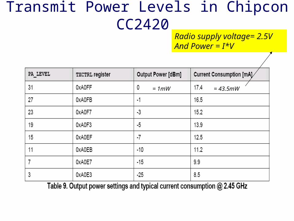
Transmit Power Levels in Chipcon CC2420

= 1mW = 43.5mW

Radio supply voltage= 2.5VAnd Power = I*V

An Experiment at Yale

XYZ sensor node designed at Yale (http://www.eng.yale.edu/enalab/XYZ)

CC2420 wireless radio from Chipcon

2.4 GHz IEEE 802.5.14/Zigbee-ready RF transceiver

DSSS modem with 9 dB spreading gain

Effective data rate: 250 Kbps

8 discrete power levels: 0, -1, -3, -5 , -7, -10, -15 and -25 dBm

Power consumption: 29mW – 52mW

Monopole antenna with length equal to 1.1inch.

EWSN 2006 February 15th Dimitrios Lymberopoulos

Received Signal Strength Indicator (RSSI)

P = RSSI + RSSIOFFSET [dBm]

The power P at the input RF pins can be obtained directly from RSSI:

RSSI is an 8-bit value computed by the radio over 8 symbols (128μs)

RSSIOFFSET is determined experimentally based on the front-end gain. It is equal to -45dbm for the CC2420 radio

Sources of RSSI Variability

Intrinsic

Radio transmitter and receiver calibration

Extrinsic

Antenna orientation

Multipath, Fading, Shadowing


Path Loss Prediction Model

Log-normal shadowing signal propagation model:

RSSI(d) = PT – PL(d0) – 10ηlog10(d/d0) + Xσ

0 5 10 15 20 25-45

-40

-35

-30

-25

-20

Distance(feet)

RS

SI

(db

m)

Averaged RSSI valueslog-fit

RSSI(d) is the RSSI value recorded at distance d

PT is the transmission power

PL(d0) is the path loss for a reference distance d0

η is the path loss exponent

Xσ is a gaussian random variable with zero mean and σ2 variance

Model verification using data from a basketball court


Radio Calibration

0-90-180-270-

0-90-180-270-

0-90-180-270-

0-90-180-270-

0-90-180-270-

0-90-180-270-

0-90-180-270-

0-90-180-270-

Receiver

1.31ftTransmitter

For each location and orientation 20 packets were sent @ -15dBm


Tra

nsm

itter

Radio Calibration

0-90-180-270-

0-90-180-270-

0-90-180-270-

0-90-180-270-

0-90-180-270-

0-90-180-270-

0-90-180-270-

0-90-180-270-

Receiver

1.31ft



Radio Calibration

0-90-180-270-

0-90-180-270-

0-90-180-270-

0-90-180-270-

0-90-180-270-

0-90-180-270-

0-90-180-270-

0-90-180-270-

Receiver

1.31ft

Transmitter



Radio Calibration

0-90-180-270-

0-90-180-270-

0-90-180-270-

0-90-180-270-

0-90-180-270-

0-90-180-270-

0-90-180-270-

0-90-180-270-

Receiver

1.31ft

Tra

nsm

itter



Radio Calibration

Experiment in an empty room

TX calibration: 9 different transmitters

RX calibration: 6 different receivers

1 2 3 4 5 6 7 8 90

5

10

15

20

25

30

350 Degrees

Transmitter ID

RSSI(

dbm

)

1 2 3 4 5 6 7 8 90

5

10

15

20

25

30

3590 Degrees

Transmitter ID

RSSI(

dbm

)

1 2 3 4 5 6 7 8 90

5

10

15

20

25

30

35180 Degrees

Transmitter ID

RSSI(

dbm

)

1 2 3 4 5 6 7 8 90

5

10

15

20

25

30

35270 Degrees

Transmitter ID

RSSI(

dbm

)

1 2 3 4 50

5

10

15

20

25

300 Degrees

Receiver ID

RSSI(

dbm

)

1 2 3 4 50

5

10

15

20

25

3090 Degrees

Receiver ID

RSSI(

dbm

)

1 2 3 4 50

5

10

15

20

25

30180 Degrees

Receiver ID

RSSI(

dbm

)

1 2 3 4 50

5

10

15

20

25

30270 Degrees

Receiver ID

RSSI(

dbm

)

TX Standard Deviation: 2.24dBm RX Standard Deviation: 1.86dBm


Antenna Characterization

Side View

8ft6.5ft

3.5ft1.25ft

Top View

2ft

2ft

2ft

: measurement point


Experiment took place in a basketball court

Minimize multipath effect

At each measurement point 20 packets @ -15dBm were received


0 2 4 6 8 10 12 14 16-50

-45

-40

-35

-30

-25

-20

-15

-10

-5

Distance (ft)

RS

SI

(db

m)

Optimal AntennaSuboptimal Antenna

Optimal antenna length-1.1inch

Random RSSI values due to multipath

Large communication range

Suboptimal antenna with 2.9inch length



5 10 15 20 25 30-48

-46

-44

-42

-40

-38

-36

-34

Distance(feet)

RS

SI

(db

m)

04590135180225270315

0 5 10 15 20 25 30-48

-46

-44

-42

-40

-38

-36

-34

-32

-30

Distance(feet)

RS

SI

(db

m)

04590135180225270315

0 5 10 15 20 25-45

-40

-35

-30

-25

-20

Distance(feet)

RS

SI

(db

m)

04590135180225270315

Similar distances (<1ft difference) can produce very different RSSI values (even up to 11dBm)

Very different distances ( even >18ft) can produce the same RSSI values


1.25ft 3.5ft 6.5ft


0 5 10 15 20 25-45

-40

-35

-30

-25

-20

Distance(feet)

RS

SI

(db

m)

6.5ft3.5ft1.5ft

0 5 10 15 20 25-50

-45

-40

-35

-30

-25

Distance(feet)

RS

SI

(db

m)

6.5ft3.5ft1.5ft

Best antenna orientation Worst antenna orientation


Antenna orientation effect

For a given height of the receiver very different RSSI values are recorded for different antenna orientations

Antenna Radiation Pattern

Side View Top View

Communication rangeSymmetric Region Antenna orientation

independent regions

Communication range

Antenna Effects in Indoor Environments

The basketball court experiment was performed inside our lab

We focused on the best antenna orientation

0 2 4 6 8 10 12 14 16-50

-45

-40

-35

-30

-25

-20

Distance (ft)

RS

SI

(db

m)

6.17ft 5.65ft 4.6ft 1.25ft


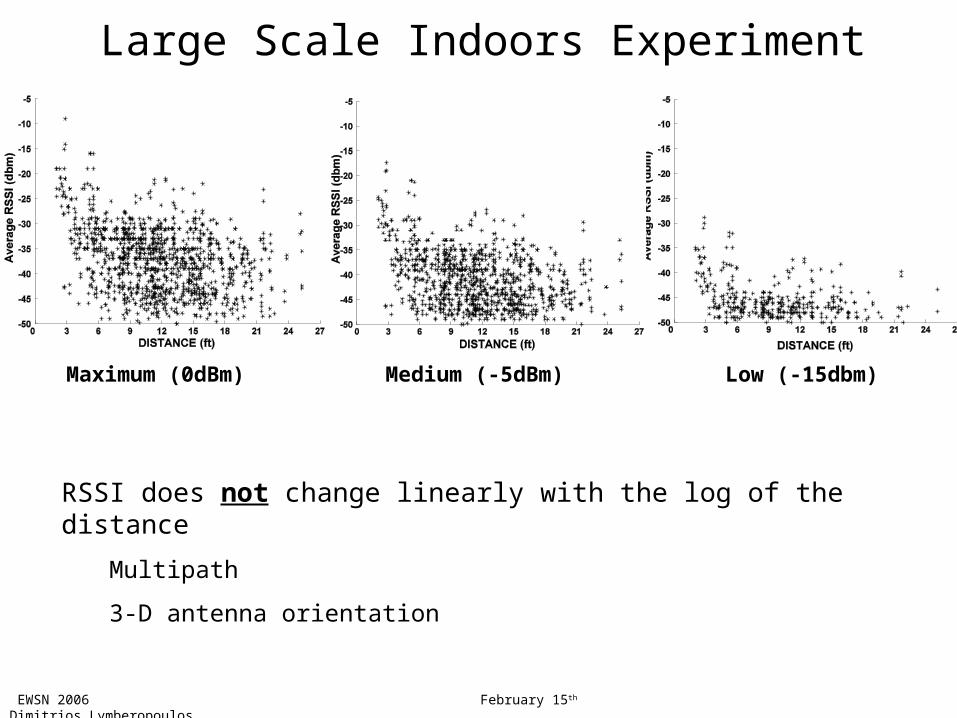
Large Scale Indoors Experiment

40 nodes were placed on the testbed (15ft (W) x 20ft(L) x 10ft(H))

Each node transmitted 10 packets at each one of the 8 power levels. The recorded RSSI values were transmitted to a base station for logging.

01

23

45

6

0

1

2

3

4

50

0.5

1

1.5

2

2.5

7

8

9

6

27

10

5

28

12

X coordinate

42

33

4

30

35

29

11

13

14

3

34

32

37

36

17

31

Connectivity at Power Level 7

41

25

15

1

2

3839

18

26

24

16

Y coordinate

40

19

22

23

20

21

Z c

oo

rdin

ate

01

23

45

6

0

1

2

3

4

50

0.5

1

1.5

2

2.5

7

8

9

6

27

10

5

28

12

X coordinate

42

33

4

30

35

29

11

13

14

3

34

32

37

36

17

31

Connectivity at Power Level 4

41

25

15

1

2

38

39

18

26

24

16

Y coordinate

40

19

22

23

20

21

Z c

oo

rdin

ate

Placement and Connectivity


Large Scale Indoors Experiment

RSSI does not change linearly with the log of the distance

Multipath

3-D antenna orientation


Maximum (0dBm) Medium (-5dBm) Low (-15dbm)

Link Asymmetry

Asymmetric link between nodes A and B

RSSI(A) ≠ RSSI(B)

1 2 3 4 5 6 7 820

22

24

26

28

30

32

34

36

Power Level (1= Maximum)

Per

cen

tag

e o

f O

ne-

Way

Lin

ks

One way Links

1 2 3 4 5 6 7 820

25

30

35

40

45

50

55

Power Level (1 = Maximum)

Per

cen

tag

e o

f as

sym

etri

c li

nks

>=2 >=3 >=4 >=5 >=6

One way links Asymmetric links


What else can we do?

More than 30% of the links are affected by human presence or motion

Detection of:

Human presence

Human motion


Experiment Lessons

3-D space is very different than 2-D space

Antenna orientation effects are dominant in 3-D deployments

3-D deployments are a more realistic for evaluating RSSI localization methods

RSSI distance prediction in 3-D deployments is almost impossible

Ordering of the RSSI values is not helpful

Even if antenna orientation is known!

Probabilistic approaches

A probabilistic model of RSSI exists for the symmetric region of the antenna

Generalizing this model to 3-D deployments is extremely difficult if not impossible.

Radio calibration has minimal effect on localization


The IEEE 802.15.4 MAC Protocol

Based on an IEEE standard for WPAN• Goal: Ultra-low cost, low power radios• Support multiple configurations (e.g point-to-point, groups,

ad-hoc etc)• CSMA-CA based protocol

o Each packet can be individually acknowledged

Key features• Three types of node functionalities

o PAN Coordinator, Coordinator and Device

• Two device types o FFD – Full Function Deviceo RFD – Reduced Function Device

Frequencies and Data Rates

BAND COVERAGE DATA RATE # OF CHANNEL(S)

2.4 GHz ISM Worldwide 250 kbps 16

868 MHz Europe 20 kbps 1

915 MHz ISM Americas 40 kbps 10

Now Back to IEEE 802.15.4 MAC

MAC supports 2 topology setups: star and peer-to-peer Star topology supports beacon and no-beacon structure

• All communication done through PAN coordinator

Start Topology: The PAN Coordinator

Any FFD may establish its own network by becoming the PAN coordinator

After formation, STAR networks operate independently from neighboring networks

PAN coordinate starts sending beacons• Other devices can associate with the network

by sending an association request

Peer-to-Peer Topology

Any FFD can communicate with any other FFD, can use multihop communication• i.e this is ad-hoc networking

RFDs can participate only as peripherals• Do not have the capabilities of forwarding packets

Each device responsible for proactively searching for other devices• Once a device is found, then they can exchange

information about what devices form

Star: Optional Beacon Structure

Beacon packet transmitted by PAN Coordinator to help Synchronization of network devices. It includes:Network identifier, beacon periodicity and superframe structure

Generic Superframe Structure

GTS: Guaranteed timeSlots assigned by PANcoordinator

Star Network: Communicating with a Coordinator

Star Network: Communicating from a Coordinator

Beacon packet indicates that thereis data pending for a network device

Device sends request on a data slot

Network device has to ask coordinator if there is data pending.If there is no data pending the Coordinator will respond with a zeroLength data packet

Peer-to-Peer Data Transfer

Peer-to-peer data transfer governed by the network layer – not specified by the standard

Four types of frames the standard can use• Beacon frame – only needed by a coordinator

• Data frame – used for all data transfers

• ACK frame – confirm successful frame reception

• A MAC Command Frame – MAC peer entity controltransfers

Beacon Frame

ACK & Data Frames

ACK Frame

Data Frame

MAC Command Frame

Radio Energy Model: the Deeper Story….

Wireless communication subsystem consists of three components with substantially different characteristics

Their relative importance depends on the transmission range of the radio

Tx: Sender Rx: Receiver

ChannelIncominginformation

Outgoinginformation

TxelecE Rx

elecERFETransmit

electronicsReceive

electronicsPower

amplifier

Energy Implication

Active transceiver power consumption more related to symbol rate rather than raw data rate

To minimize power consumption:• Minimize Ton - maximize data rate• Also minimize Ion by minimizing symbol rate

Conclusion: Multilevel or M-ary signalling should be employed in the physical layer of sensor networks• i.e need to send more than 1-bit per symbol

Energy-efficient MAC protocols

WSN-specific protocols starting from 2000 (1 paper) exponential growth (2004, 16+ papers)

Classification (up to May 2004, 20 papers) the number of channels used the degree of organization between nodes the way in which a node is notified of an incoming msg

Protocol classification

Protocol Channels Organization Notification

2000

SMACS [34] FDMA frames schedule

2001

PACT [28] single frames schedule

PicoRadio [10] CDMA+tone random wakeup

2002

STEM [33] data+ctrl random wakeup

Preamble sampling [6] single random listening

Arisha [2] single frames schedule

S-MAC [36] single slots listening

PCM [18] single random listening

Low Power Listening [13] single random listening

Protocol classification

2003

Sift [17] single random listening

EMACs [15] single frames schedule

T-MAC [5] single slots listening

TRAMA [30] single frames schedule

WiseMAC [7] single random listening

2004

BMA [24] single frames schedule

Miller [27] data+tone random wakeup+list

DMAC [26] single slots listening

SS-TDMA [23] single frames schedule

LMAC [14] single frames listening

B-MAC [29] single random listening

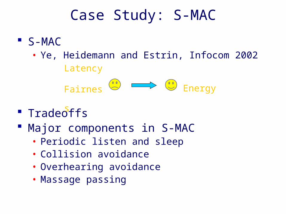
Case Study: S-MAC

S-MAC• Ye, Heidemann and Estrin, Infocom 2002

Tradeoffs Major components in S-MAC

• Periodic listen and sleep• Collision avoidance• Overhearing avoidance• Massage passing

Latency

FairnessEnergy

Coordinated Sleeping

Problem: Idle listening consumes significant energy

Solution: Periodic listen and sleep

• Turn off radio when sleeping• Reduce duty cycle to ~ 10% (120ms

on/1.2s off)

sleeplisten listen sleep

Latency Energy


Schedules can differ

• Prefer neighboring nodes have same schedule— easy broadcast & low control overhead

Border nodes: two schedules

or broadcast twice

Node 1

Node 2



Schedule 2

Schedule 1


Schedule Synchronization • New node tries to follow an existing schedule

• Remember neighbors’ schedules — to know when to send to them

• Each node broadcasts its schedule every few periods of sleeping and listening

• Re-sync when receiving a schedule update

Periodic neighbor discovery• Keep awake in a full sync interval over long periods


Adaptive listening• Reduce multi-hop latency due to periodic sleep• Wake up for a short period of time at end of each

transmission

41 2 3

CTS

RTS

CTS

Reduce latency by at least half

listen listenlisten

t1 t2

Collision Avoidance

S-MAC is based on contention Similar to IEEE 802.11 ad hoc mode (DCF)

• Physical and virtual carrier sense• Randomized backoff time• RTS/CTS for hidden terminal problem• RTS/CTS/DATA/ACK sequence

Overhearing Avoidance

Problem: Receive packets destined to others Solution: Sleep when neighbors talk

• Basic idea from PAMAS (Singh, Raghavendra 1998)• But we only use in-channel signaling

Who should sleep?• All immediate neighbors of sender and receiver

How long to sleep?• The duration field in each packet informs other

nodes the sleep interval

Message Passing

Problem: Sensor net in-network processing requires entire message

Solution: Don’t interleave different messages• Long message is fragmented & sent in burst• RTS/CTS reserve medium for entire message• Fragment-level error recovery — ACK

— extend Tx time and re-transmit immediately Other nodes sleep for whole message time

FairnessEnergy

Msg-level latency

Implementation on Testbed Nodes

Platform• Mica Motes (UC Berkeley)

o 8-bit CPU at 4MHz,o 128KB flash, 4KB RAMo 20Kbps radio at 433MHz

• TinyOS: event-driven Configurable S-MAC options

• Low duty cycle with adaptive listen• Low duty cycle without adaptive listen• Fully active mode (no periodic sleeping)

Experiments: two-hop network Topology and measured energy consumption on

source nodes

Source 1

Source 2

Sink 1

Sink 2

• S-MAC consumes much less energy than 802.11-like protocol w/o sleeping

• At heavy load, overhearing avoidance is the major factor in energy savings

• At light load, periodic sleeping plays the key role 0 2 4 6 8 10

200

400

600

800

1000

1200

1400

1600

1800Average energy consumption in the source nodes

Message inter-arrival period (second)

Ene

rgy

cons

umpt

ion

(mJ)

802.11-like protocolwithout sleep

Overhearing avoidance

S-MAC w/o adaptive listen

0 2 4 6 8 100

5

10

15

20

25

30

Message inter-arrival period (S)

En

erg

y co

nsu

mp

tion

(J)

10% duty cycle without adaptive listen

No sleep cycles

10% duty cycle with adaptive listen

Energy consumption at different traffic load

Energy Consumption over Multi-Hops

Ten-hop linear network at different traffic load

3 configurations of S-MAC

At light traffic load, periodic sleeping has significant energy savings over fully active mode

Adaptive listen saves more at heavy load by reducing latency

Latency as Hops Increase Adaptive listen significantly reduces latency

causes by periodic sleeping

0 2 4 6 8 100

2

4

6

8

10

12Latency under highest traffic load

Number of hops

Ave

rag

e m

essa

ge la

tenc

y (S

)

10% duty cycle withoutadaptive listen


No sleep cycles

0 2 4 6 8 100

2

4

6

8

10

12Latency under lowest traffic load

Number of hops

Ave

rag

e m

essa

ge la

tenc

y (S

)


10% duty cycle withadaptive listen

No sleep cycles

Throughput as Hops Increase Adaptive listen significantly increases

throughput

0 2 4 6 8 100

20

40

60

80

100

120

140

160

180

200

220Effective data throughput under highest traffic load

Number of hops

Eff

ectiv

e da

ta t

hrou

ghp

ut (

Byt

e/S

)

No sleep cycles


10% duty cycle without adaptive listen

• Using less time to pass the same amount of data

Combined Energy and Throughput

Periodic sleeping provides excellent performance at light traffic load

With adaptive listening, S-MAC achieves about the same performance as no-sleep mode at heavy load 0 2 4 6 8 10

0

0.5

1

1.5

2

2.5

3

Message inter-arrival period (S)

Ene

rgy-

time

prod

uct

per

byte

(J*

S/b

yte)

Energy-time cost on passing 1-byte data from source to sink

No sleep cycles



Documents

Introduction to Physical Layer Properties, MAC and the IEEE 802.15.4 Lecture 6 September 26, 2006 EENG 460a / CPSC 436 / ENAS 960 Networked Embedded Systems