Introduction to PDEs and Numerical Methods Lecture 11 … of lower order: subparametric functions of higher order: superparametric 𝜉= 𝑁1𝜉+ +1𝑁2𝜉=𝑁1𝜉 𝑁2𝜉

Platzhalter für Bild, Bild auf Titelfolie hinter das Logo einsetzen

Dr. Noemi Friedman, 20,27. 01. 2016.

Introduction to PDEs and Numerical Methods

Lecture 11-12.

The finite element method: assembling the matrices,

isoparametric mapping

20,27. 01 2016. | Dr. Noemi Friedman | PDE lecture| Seite 2

RECAP: How to solve PDE with

FEM with nodal basis, piecewise linear shape functions

Finite Element method with piecewise linear functions in 1D, hom DBC

1) Weak formulation of the PDE, definition of the ‚energy’ inner product (the bilinear

functional, 𝑎) and and the linear functional (𝐹)𝑎 𝑢, 𝑣 = 𝐹 𝑣

2) Define approximating subspace by definition of a mesh (nodes 0,1,..N, with coordinates,

elements) and setup the hat functions on them

3) Compute the elements of the stiffness matrix (Grammian) – evaluation of integrals

𝐾𝑖𝑗 = 𝑎 𝑁𝑖(𝑥), 𝑁𝑗(𝑥) = 𝑁𝑖(𝑥), 𝑁𝑗(𝑥) 𝐸𝑖, 𝑗 = 1. . 𝑁 − 1

4) Compute the elements of the vector of the right hand side – evaluation of integrals

𝑓𝑖 = 𝐹 𝑁𝑖 , 𝑖 = 1. . 𝑁 − 15) Solve the system of equations:

for 𝐮, which gives the solution at the nodes.

The solution in between the nodes can be calculated from:

Φ𝑖 𝑥 = Ni x =

𝑥 − 𝑥𝑖−1𝑙

𝑥 ∈ [𝑥𝑖−1, 𝑥𝑖]

𝑥𝑖+1 + 𝑥

𝑙𝑥 ∈ [𝑥𝑖 , 𝑥𝑖+1]

0 else

𝐊𝐮 = 𝐟

𝑢 x ≈

𝑖=1

𝑁

𝑢𝑖 𝑁𝑖(x)

𝑖 = 1. . 𝑁 − 1

20,27. 01 2016. | Dr. Noemi Friedman | PDE lecture | Seite 3

1D Example with linear nodal basis

𝑢 𝐱 ≈

𝑖=1

4

𝑢𝑖 𝜓𝑖(𝐱)

𝑝 𝑥 = 𝑎𝑥

Strong form:

𝑝(𝑥)

𝑙

𝑙/5 𝑙/5 𝑙/5

𝑢 0 = 𝑢 𝑙 = 0

Weak form:

0

𝑙

𝐸𝐴𝑑𝑢

𝑑𝑥

𝑑𝜓

𝑑𝑥𝑑𝑥 =

0

𝑙

𝑝 𝑥 𝜓 𝑥 𝑑𝑥

Discretisation of the weak form:

𝑖=1

4

𝑢𝑗 𝐸𝐴 𝑙

𝜕𝜓𝑖(𝑥)

𝜕𝑥

𝜕𝜓𝑗(𝑥)

𝜕𝑥𝑑𝑥 =

𝑙

𝑝(𝑥)𝜓𝑗(𝑥)𝑑𝑥

𝐾𝑖𝑗 𝑓𝑗

𝑙/5 𝑙/5

Not efficient to calculate all the

elements of the stiffness

matrix one by one!

Calculate element stiffness matrices and assemble

𝜓4 𝜓5𝜓3𝜓2



𝑝(𝑥)

𝑙

𝑙/5 𝑙/5 𝑙/5𝑙/5 𝑙/5

instead:

Compute stiffness matrix elementwisely and

then assemble

𝐊 𝐟𝐮

Global stiffness matrix

1 2 3 4 5 6

𝐾4𝑒 =

1 2 3 4 5 6

1

2

3

4

5

6

𝑢1

𝑢2

𝑢3

𝑢4

𝑢5

𝑢6

0

𝑓2

𝑓3

𝑓4

𝑓5

0

=

4 5

4

5

𝐾4𝑒 1,1 = 𝐸𝐴

Ω4

𝜕𝜓4(𝑥)

𝜕𝑥

𝜕𝜓4(𝑥)

𝜕𝑥𝑑𝑥

𝐾4𝑒(1,1) 𝐾4

𝑒(1,2)

𝐾4𝑒(2,1) 𝐾4

𝑒(2,2)


𝐾4𝑒 1,2 = 𝐸𝐴

Ω4

𝜕𝜓4(𝑥)

𝜕𝑥

𝜕𝜓5(𝑥)

𝜕𝑥𝑑𝑥

𝐾4𝑒 2,1 = 𝐸𝐴

Ω4

𝜕𝜓5(𝑥)

𝜕𝑥

𝜕𝜓4(𝑥)

𝜕𝑥𝑑𝑥

𝐾4𝑒 2,2 = 𝐸𝐴

Ω4

𝜕𝜓5(𝑥)

𝜕𝑥

𝜕𝜓5(𝑥)

𝜕𝑥𝑑𝑥

𝐾4𝑒(1,2)𝐾4

𝑒(1,1)

𝐾4𝑒(2,1) 𝐾4

𝑒(2,2)𝐾5𝑒(1,1)

𝐾3𝑒(2,2)

𝐾3𝑒 1,1𝐾2𝑒(2,2)

𝐾2𝑒 1,1𝐾1𝑒(2,2)

1

1

𝐾3𝑒(1,2)

𝐾2𝑒(1,2)

𝐾3𝑒(2,1)

𝐾2𝑒(2,1)



𝑝(𝑥)

𝑙

𝑙/5 𝑙/5 𝑙/5𝑙/5 𝑙/5

instead:

Compute stiffness matrix elementwisely and

then assemble

𝐊 𝐟𝐮

1 2 3 4 5 6

𝑓4𝑒 =

1 2 3 4 5 6

1

2

3

4

5

6

𝑢1

𝑢2

𝑢3

𝑢4

𝑢5

𝑢6

0

0

=

4

5

𝑓4𝑒 1 =

Ω4

𝑝(𝑥)𝜓4(𝑥)𝑑𝑥

𝑓4𝑒 1

𝑓4𝑒 2


𝑓4𝑒 2 =

Ω4


𝐾4𝑒(1,2)𝐾4

𝑒(1,1)

𝐾4𝑒(2,1) 𝐾4

𝑒(2,2)𝐾5𝑒(1,1)

𝐾3𝑒(2,2)

𝐾3𝑒 1,1𝐾2𝑒(2,2)

𝐾2𝑒 1,1𝐾1𝑒(2,2)

1

1

𝐾3𝑒(1,2)

𝐾2𝑒(1,2)

𝐾3𝑒(2,1)

𝐾2𝑒(2,1)

𝑓4𝑒 1

𝑓4𝑒 2

𝑓2𝑒 1

𝑓1𝑒 2

𝑓3𝑒 1

𝑓2𝑒 2

𝑓3𝑒 2

𝑓5𝑒 1

20,27. 01 2016. | Dr. Noemi Friedman | PDE lecture| Seite 6

The same but elementwisely: How to solve PDE with

FEM with nodal basis, piecewise linear shape functions

Finite Element method with piecewise linear functions in 1D, hom DBC

1) Weak formulation of the PDE, definition of the ‚energy’ inner product (the bilinear

functional, 𝑎) and and the linear functional (𝐹)𝑎 𝑢, 𝑣 = 𝐹 𝑣

2) a.) Define reference element, define maping between global and local coordinate systems

ξ 𝑥 𝑥(𝜉)

b.) Define reference linear shape functions

3) Compute the ‚element stiffness’ matrix – evaluation of integrals

𝐾𝑖𝑗 = 𝑎 𝑁𝑖(𝑥), 𝑁𝑗(𝑥) = 𝑁𝑖(𝑥), 𝑁𝑗(𝑥) 𝐸𝑖, 𝑗 = 1. . 2

4) Compute the right hand side elementwisely 𝑓𝑖𝑒 = 𝐹 𝑁𝑖 , 𝑖 = 1,2

5) Compile ‚global stiffness’ matrix

6) Solve the system of equations:

for 𝐮, which gives the solution at the nodes.

The solution in between the nodes can be calculated from:

𝐊𝐮 = 𝐟

𝑢 x ≈

𝑖=1

𝑁

𝑢𝑖 𝑁𝑖(x)

N1 ξ = 1 − ξ N2 ξ = ξ

𝐾 𝑒 = 𝐾4𝑒(1,1) 𝐾4𝑒(1,2)

𝐾4𝑒(2,1) 𝐾4

𝑒(2,2)

𝑓4𝑒 = 𝑓4

𝑒 1

𝑓4𝑒 2


Local/global coordinate system 1D

𝐾4𝑒 𝑘, 𝑙 = 𝐸𝐴

Ω4

𝜕𝑁𝑘(𝜉)

𝜕𝜉

𝜕𝜉

𝜕𝑥

𝜕𝑁𝑙(𝜉)

𝜕𝜉

𝜕𝜉

𝜕𝑥𝑑𝑥 =

𝐸𝐴

𝑙4𝑒 2

Ω4

𝜕𝑁𝑘(𝜉)

𝜕𝜉

𝜕𝑁𝑙(𝜉)

𝜕𝜉𝑑𝑥

𝜉 = [0,1]

1

𝑙𝑒

1

𝑙𝑒

𝐾4𝑒 𝑘, 𝑙 =

𝐸𝐴

𝑙 𝑒 2 0

1 𝜕𝑁𝑘(𝜉)

𝜕𝜉

𝜕𝑁𝑙(𝜉)

𝜕𝜉

𝑑𝑥(𝜉)

𝑑𝜉𝑑𝜉 =𝐸𝐴

𝑙 𝑒 0

1 𝜕𝑁𝑘(𝜉)

𝜕𝜉

𝜕𝑁𝑙(𝜉)

𝜕𝜉𝑑𝜉

𝑙 𝑒

Idea:

coordinate transformation to have unit length elements element stiffnes matrix is the same for each element

𝜕𝜉

𝜕𝑥=1

𝑙 𝑒


Ω4

𝜕𝜓4(𝑥)

𝑥

𝜕𝜓5(𝑥)

𝜕𝑥𝑑𝑥

𝑘, 𝑙 ∈ [1,2]

𝑖, 𝑗 ∈ [4,5]


Local/global coordinate system 1D

𝑓4𝑒 𝑙 =

Ω4


Ω4

𝑝(𝑥)𝜓5(𝑥)𝑑𝑥= 0

1

𝑝(𝜉)𝑁𝑙(𝜉)𝑑𝑥(𝜉)

𝑑𝜉𝑑𝜉 = 𝑙 𝑒

0

1

𝑝(𝜉)𝑁𝑙(𝜉)𝑑𝜉

𝑙 ∈ [1,2]


Local/ coordinate system, isoparametric mapping 1D

coordinate transformation

using the ansatzfunctions isoparametric mapping

functions of lower order: subparametric

functions of higher order: superparametric

𝑥 𝜉 = 𝑥𝑖𝑁1 𝜉 + 𝑥𝑖+1𝑁2 𝜉 = 𝑁1 𝜉 𝑁2 𝜉𝑥𝑖𝑥𝑖+1

local coordinate

global coordinate

𝜉 = 0 𝜉 = 1

𝑥𝑖 𝑥2

Shape functions:

Transformation from local to global coordinates:

Stiffness matrix with isoparametric elements:

𝜉 = [0,1]𝑥

𝑁1 𝜉 = 1 − 𝜉

𝑁2 𝜉 = 𝜉


Ω4

𝜕𝜓𝑖(𝑥)

𝑥

𝜕𝜓𝑗(𝑥)

𝜕𝑥𝑑𝑥 = 𝐸𝐴

Ω4

𝜕𝑁𝑘(𝜉)

𝜕𝜉

𝜕𝜉

𝜕𝑥

𝜕𝑁𝑙(𝜉)

𝜕𝜉

𝜕𝜉

𝜕𝑥𝑑𝑥

𝑘, 𝑙 ∈ [1,2]

𝑖, 𝑗 ∈ [4,5]


0

1 𝜕𝑁𝑘(𝜉)

𝜕𝜉

𝑑𝑥

𝑑𝜉

−1𝜕𝑁𝑙(𝜉)

𝜕𝜉

𝑑𝑥

𝑑𝜉

−1𝑑𝑥(𝜉)

𝑑𝜉𝑑𝜉

𝑑𝑥

𝑑𝜉= 𝑥𝑖𝑑𝑁1 𝜉

𝑑𝜉+ 𝑥𝑖+1

𝑑𝑁2 𝜉

𝑑𝜉

𝑑𝑥

𝑑𝜉=𝑑𝑁1 𝜉

𝑑𝜉

𝑑𝑁2 𝜉

𝑑𝜉

𝑥𝑖𝑥𝑖+1

𝑑𝑥

𝑑𝜉

−1 𝑑𝑥

𝑑𝜉

−1


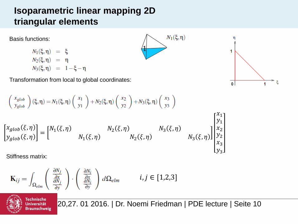
Isoparametric linear mapping 2D

triangular elements

Basis functions:

Transformation from local to global coordinates:

Stiffness matrix:

1

𝑖, 𝑗 ∈ [1,2,3]

𝑥𝑔𝑙𝑜𝑏 𝜉, 𝜂

𝑦𝑔𝑙𝑜𝑏 𝜉, 𝜂=𝑁1 𝜉, 𝜂 𝑁2 𝜉, 𝜂

𝑁1 𝜉, 𝜂

𝑁3 𝜉, 𝜂

𝑁2 𝜉, 𝜂 𝑁3 𝜉, 𝜂

𝑥1𝑦1𝑥2𝑦2𝑥3𝑦3



triangular elements

Stiffness matrix:

Stiffness matrix with local coordinates:

where:

substitution rule

determinant should not be negative or zero!

𝐉 =

𝑖=1

3𝜕𝑁𝑖 𝜉, 𝜂

𝜕𝜉𝑥𝑖

𝑖=1


𝜕𝜂𝑥𝑖

𝑖=1


𝜕𝜉𝑦𝑖

𝑖=1


𝜕𝜂𝑦𝑖

𝑖, 𝑗 ∈ [1,2,3]

𝑖, 𝑗 ∈ [1,2,3]𝑲𝑖𝑗 =

0

1

0

1−𝜂

𝑱−𝑻

𝜕𝑁𝑗

𝜕𝜉𝜕𝑁𝑗

𝜕𝜂

∙ 𝑱−𝑻

𝜕𝑁𝑖𝜕𝜉𝜕𝑁𝑖𝜕𝜂

𝑱 𝑑𝜉𝑑𝜂



triangular elements, example

𝑥 𝜉, 𝜂

𝑦 𝜉, 𝜂=1 − 𝜉 − 𝜂 𝜉

1 − 𝜉 − 𝜂

𝜂𝜉 𝜂

237197

Transformation from local to global coordinates (isoparametric mapping):

𝑥𝑔𝑙𝑜𝑏 𝜉, 𝜂

𝑦𝑔𝑙𝑜𝑏 𝜉, 𝜂=𝑁1 𝜉, 𝜂 𝑁2 𝜉, 𝜂

𝑁1 𝜉, 𝜂

𝑁3 𝜉, 𝜂

𝑁2 𝜉, 𝜂 𝑁3 𝜉, 𝜂

𝑥1𝑦1𝑥2𝑦2𝑥3𝑦3

1 2

3

4

5 6




Stiffness matrix with local coordinates:

𝑖, 𝑗 ∈ [1,2,3]𝑲𝑖𝑗 = 0

1

0

1−𝜂

𝑱−𝑻

𝜕𝑁𝑗


𝜕𝜂

∙ 𝑱−𝑻






𝑱𝑻 = 𝑱𝑻 = 𝑱 = 34𝑱 =𝟓 𝟕−𝟐 𝟒

𝑱−𝑻 =𝟏

𝑱𝑻𝟒 𝟐−𝟕 𝟓

𝑲𝑖𝑗𝑒= 0

1

0

1−𝜂 1

344 2−7 5

𝜕𝑁𝑗


𝜕𝜂

∙1

344 2−7 5


34𝑑𝜉𝑑𝜂

𝑲21𝑒= 01 01−𝜂 1

34

4 2−7 5

−1−1∙1

34

4 2−7 5

1034𝑑𝜉𝑑𝜂 == 0

1 −11−𝜂 1

34

−62∙4−7𝑑𝜉𝑑𝜂

𝑲21𝑒==−1.118 0

1 01−𝜂𝑑𝜉𝑑𝜂 = −1.118 ⋅

1

2= −0.559

𝑲𝑖𝑗𝑒= 0

1

0

1−𝜂

𝑱−𝑻

𝜕𝑁𝑗


𝜕𝜂

∙ 𝑱−𝑻



𝑲11𝑒𝑲12𝑒𝑲13𝑒






𝑱𝑻 = 𝑱 = 34𝑲11𝑒𝑲12𝑒𝑲13𝑒



𝑓𝑒 =

Ω𝑒

𝑝(𝑥)𝑁1(𝑥, 𝑦)𝑑𝑥

Ω𝑒


Ω𝑒


=

0

1

0

1−𝜂

𝑝(𝜉)𝑁1(𝜉, 𝜂) 𝑱 𝑑𝜉𝑑𝜂

0

1

0

1−𝜂


0

1

0

1−𝜂


𝑢1𝑒

𝑢2𝑒

𝑢3𝑒

𝑓1𝑒

𝑓2𝑒

𝑓3𝑒

=







𝑢1𝑒

𝑢2𝑒

𝑢3𝑒

𝑓1𝑒

𝑓2𝑒

𝑓3𝑒

=

1 2

3

4

5

local 1 2 3global 4 3 6

6

𝑲22𝑒𝑲21𝑒

𝑲23𝑒


𝑲13𝑒


𝑲33𝑒

𝑢1

𝑢2

𝑢3

𝑢4

𝑢5

𝑢6

𝑓2𝑒

𝑓1𝑒

𝑓3𝑒

4

3

6

1

2

3

4

5

6

1

2

3

1 2 3 4 5 6

=

4

3

6

Documents

Introduction to PDEs and Numerical Methods Lecture 11 … of lower order: subparametric functions of higher order: superparametric 𝜉= 𝑁1𝜉+ +1𝑁2𝜉=𝑁1𝜉 𝑁2𝜉