Embed Size (px)
Citation preview

Introduction to Computational Linguisyicshttp://www-rohan.sdsu.edu/~gawron/compling
Naive Bayes
Gawron
Department of Linguistics, San Diego State University
2011-04-08
Jean Mark Gawron ( San Diego State University )Jean Mark Gawron: Naive Bayes 2011-04-08 1 / 33

Overview
1 Sense disambiguation
2 Naive Bayes
3 NB theory
Jean Mark Gawron ( San Diego State University )Jean Mark Gawron: Naive Bayes 2011-04-08 2 / 33

An ambiguous word
Jean Mark Gawron ( San Diego State University )Jean Mark Gawron: Naive Bayes 2011-04-08 3 / 33

Examples
He plays the bass well.
He caught a huge bass.
They served fried bass for lunch.
She carried her bass clarinet into class.
Charlie is the bass in a barbershop quartet.
Jean Mark Gawron ( San Diego State University )Jean Mark Gawron: Naive Bayes 2011-04-08 4 / 33

The Naive Bayes classifier
The Naive Bayes classifier is a probabilistic classifier.
We will estimate the probability of a word like bass in a document dbeing a use of word sense s as follows:
P(s | d) ∝ P(s)∏
1≤k≤nd
P(tk | s)
where nd is the number of context features in document d , takenfrom a set of context features (words) for disambiguating bass.
P(tk |s) is the conditional probability of context feature tk occurringin the same document with sense s.
P(tk |s) as a measure of how much evidence tk contributes that s isthe correct sense.
P(s) is the prior probability of sense s.
If a context does not provide clear evidence for one sense vs. another,we choose the s with highest P(s).
Jean Mark Gawron ( San Diego State University )Jean Mark Gawron: Naive Bayes 2011-04-08 5 / 33
Maximum a posteriori class
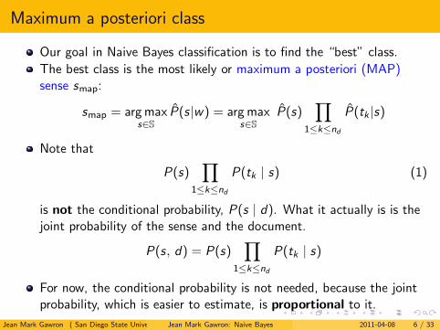
Our goal in Naive Bayes classification is to find the “best” class.
The best class is the most likely or maximum a posteriori (MAP)sense smap:
smap = argmaxs∈S
P̂(s|w) = arg maxs∈S
P̂(s)∏
1≤k≤nd
P̂(tk |s)
Note that
P(s)∏
1≤k≤nd
P(tk | s) (1)
is not the conditional probability, P(s | d). What it actually is is thejoint probability of the sense and the document.
P(s, d) = P(s)∏
1≤k≤nd
P(tk | s)
For now, the conditional probability is not needed, because the jointprobability, which is easier to estimate, is proportional to it.
Jean Mark Gawron ( San Diego State University )Jean Mark Gawron: Naive Bayes 2011-04-08 6 / 33
Taking the log
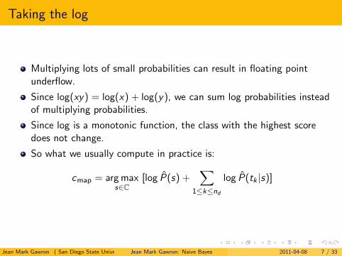
Multiplying lots of small probabilities can result in floating pointunderflow.
Since log(xy) = log(x) + log(y), we can sum log probabilities insteadof multiplying probabilities.
Since log is a monotonic function, the class with the highest scoredoes not change.
So what we usually compute in practice is:
cmap = argmaxs∈C
[log P̂(s) +∑
1≤k≤nd
log P̂(tk |s)]
Jean Mark Gawron ( San Diego State University )Jean Mark Gawron: Naive Bayes 2011-04-08 7 / 33

Naive Bayes classifier
Jean Mark Gawron ( San Diego State University )Jean Mark Gawron: Naive Bayes 2011-04-08 8 / 33

Naive Bayes classifier
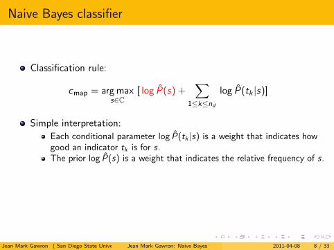
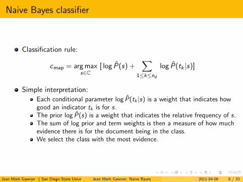
Classification rule:
cmap = argmaxs∈C
[ log P̂(s) +∑
1≤k≤nd
log P̂(tk |s)]
Jean Mark Gawron ( San Diego State University )Jean Mark Gawron: Naive Bayes 2011-04-08 8 / 33

Naive Bayes classifier
Classification rule:
cmap = argmaxs∈C
[ log P̂(s) +∑
1≤k≤nd
log P̂(tk |s)]
Simple interpretation:
Jean Mark Gawron ( San Diego State University )Jean Mark Gawron: Naive Bayes 2011-04-08 8 / 33

Naive Bayes classifier
Classification rule:
cmap = argmaxs∈C
[ log P̂(s) +∑
1≤k≤nd
log P̂(tk |s)]
Simple interpretation:
Each conditional parameter log P̂(tk |s) is a weight that indicates howgood an indicator tk is for s.
Jean Mark Gawron ( San Diego State University )Jean Mark Gawron: Naive Bayes 2011-04-08 8 / 33
Naive Bayes classifier
Classification rule:
cmap = argmaxs∈C
[ log P̂(s) +∑
1≤k≤nd
log P̂(tk |s)]
Simple interpretation:
Each conditional parameter log P̂(tk |s) is a weight that indicates howgood an indicator tk is for s.The prior log P̂(s) is a weight that indicates the relative frequency of s.
Jean Mark Gawron ( San Diego State University )Jean Mark Gawron: Naive Bayes 2011-04-08 8 / 33

Naive Bayes classifier
Classification rule:
cmap = argmaxs∈C
[ log P̂(s) +∑
1≤k≤nd
log P̂(tk |s)]
Simple interpretation:
Each conditional parameter log P̂(tk |s) is a weight that indicates howgood an indicator tk is for s.The prior log P̂(s) is a weight that indicates the relative frequency of s.The sum of log prior and term weights is then a measure of how muchevidence there is for the document being in the class.
Jean Mark Gawron ( San Diego State University )Jean Mark Gawron: Naive Bayes 2011-04-08 8 / 33
Naive Bayes classifier
Classification rule:
cmap = argmaxs∈C
[ log P̂(s) +∑
1≤k≤nd
log P̂(tk |s)]
Simple interpretation:
Each conditional parameter log P̂(tk |s) is a weight that indicates howgood an indicator tk is for s.The prior log P̂(s) is a weight that indicates the relative frequency of s.The sum of log prior and term weights is then a measure of how muchevidence there is for the document being in the class.We select the class with the most evidence.
Jean Mark Gawron ( San Diego State University )Jean Mark Gawron: Naive Bayes 2011-04-08 8 / 33

Parameter estimation take 1: Maximum likelihood
Jean Mark Gawron ( San Diego State University )Jean Mark Gawron: Naive Bayes 2011-04-08 9 / 33

Parameter estimation take 1: Maximum likelihood
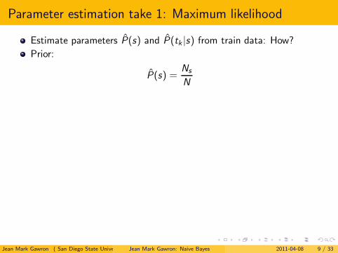
Estimate parameters P̂(s) and P̂(tk |s) from train data: How?
Jean Mark Gawron ( San Diego State University )Jean Mark Gawron: Naive Bayes 2011-04-08 9 / 33
Parameter estimation take 1: Maximum likelihood
Estimate parameters P̂(s) and P̂(tk |s) from train data: How?
Prior:
P̂(s) =Ns
N
Jean Mark Gawron ( San Diego State University )Jean Mark Gawron: Naive Bayes 2011-04-08 9 / 33

Parameter estimation take 1: Maximum likelihood
Estimate parameters P̂(s) and P̂(tk |s) from train data: How?
Prior:
P̂(s) =Ns
N
Ns : number of tokens of word w using sense s; N: total number oftokens of word w .
Conditional probabilities:
P̂(t|s) =Tst∑
t′∈V Tst′
Tst is the number of tokens of t in training data with sense s
(includes multiple occurrences)
We’ve made a Naive Bayes independence assumption here:
P̂(tj , tk |s) = P̂(tj |s)P̂(tk |s, tj ) = P̂(tj |s)P̂(tk |s)
Jean Mark Gawron ( San Diego State University )Jean Mark Gawron: Naive Bayes 2011-04-08 9 / 33

The problem with maximum likelihood estimates: Zeros
Jean Mark Gawron ( San Diego State University )Jean Mark Gawron: Naive Bayes 2011-04-08 10 / 33

The problem with maximum likelihood estimates: Zeros
S=bassfish
X1=play X2=play X3=salmon X4=fry X5=hook
P(bassfish|d) ∝ P(bassfish) · P(play|bassfish) · P(play|bassfish)
· P(salmon|bassfish) · P(fry|bassfish) · P(hook|bassfish)
If hook never occurs with sense bassfish in the training set:
P̂(hook|bassfish) =Tbassfish,hook∑t′∈V Tbassfish,t′
=0∑
t′∈V Tbassfish,t′= 0
Jean Mark Gawron ( San Diego State University )Jean Mark Gawron: Naive Bayes 2011-04-08 10 / 33
The problem with maximum likelihood estimates: Zeros
(cont)
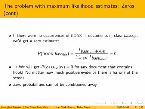
If there were no occurrences of hook in documents in class bassfish,we’d get a zero estimate:
P̂(hook|bassfish) =Tbassfish,hook∑t′∈V Tbassfish,t′
= 0
→ We will get P(bassfish|w) = 0 for any document that containshook! No matter how much positive evidence there is for one of thesenses.
Zero probabilities cannot be conditioned away.
Jean Mark Gawron ( San Diego State University )Jean Mark Gawron: Naive Bayes 2011-04-08 11 / 33

To avoid zeros: Add-one smoothing
Jean Mark Gawron ( San Diego State University )Jean Mark Gawron: Naive Bayes 2011-04-08 12 / 33

To avoid zeros: Add-one smoothing
Before:
P̂(t|s) =Tst∑
t′∈V Tst′
Jean Mark Gawron ( San Diego State University )Jean Mark Gawron: Naive Bayes 2011-04-08 12 / 33

To avoid zeros: Add-one smoothing
Before:
P̂(t|s) =Tst∑
t′∈V Tst′
Now: Add one to each count to avoid zeros:
P̂sm(t|s) =Tst + 1∑
t′∈Vw(Tct′ + 1)
=Tst + 1
(∑
t′∈V Tst′) + |Vw |
Jean Mark Gawron ( San Diego State University )Jean Mark Gawron: Naive Bayes 2011-04-08 12 / 33

To avoid zeros: Add-one smoothing
Before:
P̂(t|s) =Tst∑
t′∈V Tst′
Now: Add one to each count to avoid zeros:
P̂sm(t|s) =Tst + 1∑
t′∈Vw(Tct′ + 1)
=Tst + 1
(∑
t′∈V Tst′) + |Vw |
Vw is the set of context features for w (bass, the word we aredisambiguating), and |Vw | is the number of such features.
Jean Mark Gawron ( San Diego State University )Jean Mark Gawron: Naive Bayes 2011-04-08 12 / 33

Naive Bayes: Summary
Jean Mark Gawron ( San Diego State University )Jean Mark Gawron: Naive Bayes 2011-04-08 13 / 33

Naive Bayes: Summary
Estimate parameters from the training corpus using add-onesmoothing
Jean Mark Gawron ( San Diego State University )Jean Mark Gawron: Naive Bayes 2011-04-08 13 / 33

Naive Bayes: Summary
Estimate parameters from the training corpus using add-onesmoothing
For a new document, for each class, compute sum of (i) log of priorand (ii) logs of conditional probabilities of the terms
Assign the document to the class with the largest score
Jean Mark Gawron ( San Diego State University )Jean Mark Gawron: Naive Bayes 2011-04-08 13 / 33

Naive Bayes: Training
TrainMultinomialNB(S,D,w)1 V ← ExtractFeatures(D,w)2 N ← CountOccurrences(D,w)3 for each s ∈ S
4 do Ns ← CountOccurrencesOfSense(D, s)5 prior [s]← Ns/N6 texts ← ConcatTextOfAllContextsWithSense(D, s)7 for each t ∈ V
8 do Tst ← CountTokensOfTerm(texts , t)9 for each t ∈ V
10 do condprob[t][s]← Tst+1∑t′ (Tst′+1)
11 return V , prior , condprob
Jean Mark Gawron ( San Diego State University )Jean Mark Gawron: Naive Bayes 2011-04-08 14 / 33

Naive Bayes: Testing
ApplyMultinomialNB(S,V , prior , condprob, d)1 W ← ExtractFeatureTokensFromDoc(V , d)2 for each s ∈ S
3 do score[c]← log prior [s]4 for each t ∈W
5 do score[s]+ = log condprob[t][s]6 return argmaxs∈S score[s]
Jean Mark Gawron ( San Diego State University )Jean Mark Gawron: Naive Bayes 2011-04-08 15 / 33

Exercise
For our feature set, we often choose the n most frequent content words in ourdocument set, retaining duplicates, leaving out w (bass). Here we choose fry, play,
clarinet, salmon, hook, and guitar. Note that guitar occurs in neither the test set nortraining set. Assume the context window for training
docID words in context in s = bassfish?
training set 1 fry fry yes2 play play clarinet no3 salmon fry yes4 play yes
test set 5 play play fry hook play play play play play ?
Estimate parameters of Naive Bayes classifierClassify test document
Jean Mark Gawron ( San Diego State University )Jean Mark Gawron: Naive Bayes 2011-04-08 16 / 33
Unsmoothed Example: Parameter estimates
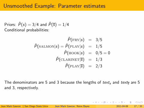
Priors: P̂(s) = 3/4 and P̂(s) = 1/4Conditional probabilities:
P̂(fry|s) = 3/5
P̂(salmon|s) = P̂(play|s) = 1/5
P̂(hook|s) = 0/5 = 0
P̂(clarinet|s) = 1/3
P̂(play|s) = 2/3
The denominators are 5 and 3 because the lengths of texts and texts are 5and 3, respectively.
Jean Mark Gawron ( San Diego State University )Jean Mark Gawron: Naive Bayes 2011-04-08 17 / 33

Smoothing Example: Parameter estimates
Priors: P̂(s) = 3/4 and P̂(s) = 1/4Conditional probabilities:
P̂sm(fry|s) = (3 + 1)/(5 + 6) = 4/11
P̂sm(salmon|s) = P̂sm(play|s) = (1 + 1)/(5 + 6) = 2/11
P̂sm(hook|s) = (0 + 1)/(5 + 6) = 1/11
P̂sm(clarinet|s) = (1 + 1)/(3 + 6) = 2/9
P̂sm(play|s) = (2 + 1)/(3 + 6) = 3/9 = 1/3
The denominators are (5 + 6) and (3 + 6) because the lengths of texts andtexts are 5 and 3, respectively, and because the constant |Vw | is 6 as thefeature set consists of six terms.
Jean Mark Gawron ( San Diego State University )Jean Mark Gawron: Naive Bayes 2011-04-08 18 / 33

Example: Classification
P̂sm(s|d5) ∝ 3/4 · (2/11)7 · 4/11 · 1/11 ≈ 1.643 ∗ 10−7
P̂sm(s |d5) ∝ 1/4 · (1/3)7 · 1/9 · 1/9 ≈ 2.389 ∗ 10−7
Thus, the classifier assigns the test document to s = bassfish.The reason for this classification decision is that the seven occurrences ofthe negative indicator play in d5 outweigh the occurrence the positiveindicator fry.Note: the terms to the right of ∝ are what we were referring to as jointprobabilities in first few slides.
Jean Mark Gawron ( San Diego State University )Jean Mark Gawron: Naive Bayes 2011-04-08 19 / 33

Normalizing Joint probabilities
To get from joint probability P̂(s1, t1,nd ) to the conditional probabilityP̂(s1 | t1,nd ) we must normalize:
(a) P̂(s1, t1,nd ) = P̂(s)∏
1≤k≤ndP̂(tk |s1) = 0.00099
(b) P̂(s1|t1,nd ) = P̂(s1, t1,nd )/P̂(d)
(c) P̂(s2, t1,nd ) = P̂(s)∏
1≤k≤ndP̂(tk |s1) = 0.00001
(d) P̂(s2|t1,nd ) = P̂(s2, t1,nd )/P̂(d)
(e) P̂(s1|t1,nd ) + P̂(s2|t1,nd ) =P̂(s1,t1,nd )+P̂(s2,t1,nd )
P̂(d)= 1.0
(f) P̂(s1, t1,nd ) + P̂(s2, t1,nd ) = P̂(d) = 0.0001
(g) P̂(s1|t1,nd ) = 0.99, P̂(s2|t1,nd ) = 0.01.
Jean Mark Gawron ( San Diego State University )Jean Mark Gawron: Naive Bayes 2011-04-08 20 / 33

How to normalize
P̂(s1|t1,nd ) =P̂(s1, t1,nd )∑i P̂(si , t1,nd )
In our example there are only two senses, so:
P̂(s1|t1,nd ) =P̂(s1, t1,nd )
P̂(s1, t1,nd ) + P̂(s2, t1,nd )=
.00099
.00099 + .00001=
.00099
.001= .99.
SinceP̂)(t1,nd ) =
∑
si
P̂(si , t1,nd ) = P̂(s1, t1,nd ) + P̂(s2, t1,nd )
this is just a rewrite of our definition of conditional probability:
P̂(s1|t1,nd ) =P̂(s1, t1,nd )
P̂(t1,nd )
Jean Mark Gawron ( San Diego State University )Jean Mark Gawron: Naive Bayes 2011-04-08 21 / 33

Time complexity of Naive Bayes
Jean Mark Gawron ( San Diego State University )Jean Mark Gawron: Naive Bayes 2011-04-08 22 / 33

Time complexity of Naive Bayes
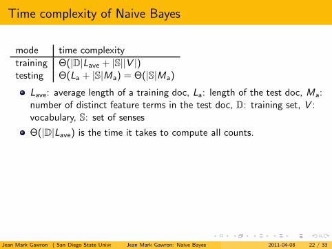
mode time complexity
training Θ(|D|Lave + |S||V |)testing Θ(La + |S|Ma) = Θ(|S|Ma)
Lave: average length of a training doc, La: length of the test doc, Ma:number of distinct feature terms in the test doc, D: training set, V :vocabulary, S: set of senses
Jean Mark Gawron ( San Diego State University )Jean Mark Gawron: Naive Bayes 2011-04-08 22 / 33
Time complexity of Naive Bayes
mode time complexity
training Θ(|D|Lave + |S||V |)testing Θ(La + |S|Ma) = Θ(|S|Ma)
Lave: average length of a training doc, La: length of the test doc, Ma:number of distinct feature terms in the test doc, D: training set, V :vocabulary, S: set of senses
Θ(|D|Lave) is the time it takes to compute all counts.
Jean Mark Gawron ( San Diego State University )Jean Mark Gawron: Naive Bayes 2011-04-08 22 / 33

Time complexity of Naive Bayes
mode time complexity
training Θ(|D|Lave + |S||V |)testing Θ(La + |S|Ma) = Θ(|S|Ma)
Lave: average length of a training doc, La: length of the test doc, Ma:number of distinct feature terms in the test doc, D: training set, V :vocabulary, S: set of senses
Θ(|D|Lave) is the time it takes to compute all counts.
Θ(|S||V |) is the time it takes to compute the parameters from thecounts.
Generally: |S||V | < |D|Lave
Test time is also linear (in the length of the test document).
Thus: Naive Bayes is linear in the size of the training set (training)and the test document (testing). This is optimal.
Jean Mark Gawron ( San Diego State University )Jean Mark Gawron: Naive Bayes 2011-04-08 22 / 33

Naive Bayes: Analysis
Jean Mark Gawron ( San Diego State University )Jean Mark Gawron: Naive Bayes 2011-04-08 23 / 33

Naive Bayes: Analysis
Now we want to gain a better understanding of the properties ofNaive Bayes.
Jean Mark Gawron ( San Diego State University )Jean Mark Gawron: Naive Bayes 2011-04-08 23 / 33

Naive Bayes: Analysis
Now we want to gain a better understanding of the properties ofNaive Bayes.
We will formally derive the classification rule . . .
Jean Mark Gawron ( San Diego State University )Jean Mark Gawron: Naive Bayes 2011-04-08 23 / 33

Naive Bayes: Analysis
Now we want to gain a better understanding of the properties ofNaive Bayes.
We will formally derive the classification rule . . .
. . . and state the assumptions we make in that derivation explicitly.
Jean Mark Gawron ( San Diego State University )Jean Mark Gawron: Naive Bayes 2011-04-08 23 / 33

Derivation of Naive Bayes rule
Jean Mark Gawron ( San Diego State University )Jean Mark Gawron: Naive Bayes 2011-04-08 24 / 33

Derivation of Naive Bayes rule
We want to find the class that is most likely given the document:
cmap = argmaxs∈C
P(s|d)
Apply Bayes rule P(A|B) = P(B|A)P(A)P(B) :
cmap = argmaxs∈C
P(d |s)P(s)
P(d)
Drop denominator since P(d) is the same for all classes:
cmap = argmaxs∈C
P(d |s)P(s)
Jean Mark Gawron ( San Diego State University )Jean Mark Gawron: Naive Bayes 2011-04-08 24 / 33

Too many parameters / sparseness
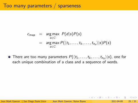
cmap = argmaxs∈C
P(d |s)P(s)
= argmaxs∈C
P(〈t1, . . . , tk , . . . , tnd 〉|s)P(s)
Jean Mark Gawron ( San Diego State University )Jean Mark Gawron: Naive Bayes 2011-04-08 25 / 33
Too many parameters / sparseness
cmap = argmaxs∈C
P(d |s)P(s)
= argmaxs∈C
P(〈t1, . . . , tk , . . . , tnd 〉|s)P(s)
There are too many parameters P(〈t1, . . . , tk , . . . , tnd 〉|s), one foreach unique combination of a class and a sequence of words.
Jean Mark Gawron ( San Diego State University )Jean Mark Gawron: Naive Bayes 2011-04-08 25 / 33

Too many parameters / sparseness
cmap = argmaxs∈C
P(d |s)P(s)
= argmaxs∈C
P(〈t1, . . . , tk , . . . , tnd 〉|s)P(s)
There are too many parameters P(〈t1, . . . , tk , . . . , tnd 〉|s), one foreach unique combination of a class and a sequence of words.
We would need a very, very large number of training examples toestimate that many parameters.
This is the problem of data sparseness.
Jean Mark Gawron ( San Diego State University )Jean Mark Gawron: Naive Bayes 2011-04-08 25 / 33

Naive Bayes conditional independence assumption
To reduce the number of parameters to a manageable size, we make theNaive Bayes conditional independence assumption:
P(d |s) = P(〈t1, . . . , tnd 〉|s) =∏
1≤k≤nd
P(Xk = tk |s)
We assume that the probability of observing the conjunction of attributesis equal to the product of the individual probabilities P(Xk = tk |s).Recall from earlier the estimates for these priors and conditionalprobabilities: P̂(s) = Nc
Nand P̂(t|c) = Tct+1
(∑
t′∈V Tct′)+B
Jean Mark Gawron ( San Diego State University )Jean Mark Gawron: Naive Bayes 2011-04-08 26 / 33

Generative Model
S=bassfish
X1=play X2=clarinet X3=salmon X4=fry X5=hook
P(s|d) ∝ P(s)∏
1≤k≤|nd |P(tk |c)
Jean Mark Gawron ( San Diego State University )Jean Mark Gawron: Naive Bayes 2011-04-08 27 / 33

Generative Model
S=bassfish
X1=play X2=clarinet X3=salmon X4=fry X5=hook
P(s|d) ∝ P(s)∏
1≤k≤|nd |P(tk |c)
Generate a sense with probability P(s)
Jean Mark Gawron ( San Diego State University )Jean Mark Gawron: Naive Bayes 2011-04-08 27 / 33

Generative Model
S=bassfish
X1=play X2=clarinet X3=salmon X4=fry X5=hook
P(s|d) ∝ P(s)∏
1≤k≤|nd |P(tk |c)
Generate a sense with probability P(s)
Generate each of the context words, conditional on the sense, butindependent of each other, with probability P(tk |s)
To classify docs, we “simulate” the generative process and find thesense that is most likely to have generated the doc.
Jean Mark Gawron ( San Diego State University )Jean Mark Gawron: Naive Bayes 2011-04-08 27 / 33

Second independence assumption
Jean Mark Gawron ( San Diego State University )Jean Mark Gawron: Naive Bayes 2011-04-08 28 / 33

Second independence assumption
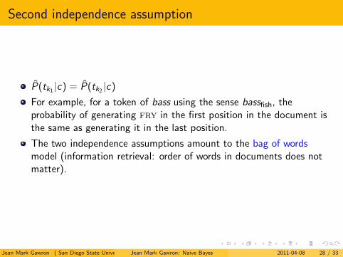
P̂(tk1 |c) = P̂(tk2 |c)
Jean Mark Gawron ( San Diego State University )Jean Mark Gawron: Naive Bayes 2011-04-08 28 / 33

Second independence assumption
P̂(tk1 |c) = P̂(tk2 |c)
For example, for a token of bass using the sense bassfish, theprobability of generating fry in the first position in the document isthe same as generating it in the last position.
Jean Mark Gawron ( San Diego State University )Jean Mark Gawron: Naive Bayes 2011-04-08 28 / 33
Second independence assumption
P̂(tk1 |c) = P̂(tk2 |c)
For example, for a token of bass using the sense bassfish, theprobability of generating fry in the first position in the document isthe same as generating it in the last position.
The two independence assumptions amount to the bag of wordsmodel (information retrieval: order of words in documents does notmatter).
Jean Mark Gawron ( San Diego State University )Jean Mark Gawron: Naive Bayes 2011-04-08 28 / 33

A different Naive Bayes model: Bernoulli model
Uplay=0 Uclarinet=1 Usalmon=0 U fry=1 Uhook=1
C=bassfish
multinomial cmap = argmaxs∈C [log P̂(s) +∑
1≤k≤|nd |log P̂(tk |s)]
bernoulli cmap = argmaxs∈C [log P̂(s) +∑
1≤k≤|Vw |log P̂(tk |s)]
Jean Mark Gawron ( San Diego State University )Jean Mark Gawron: Naive Bayes 2011-04-08 29 / 33

Violation of Naive Bayes independence assumptions
Jean Mark Gawron ( San Diego State University )Jean Mark Gawron: Naive Bayes 2011-04-08 30 / 33
Violation of Naive Bayes independence assumptions
The independence assumptions do not really hold of documentswritten in natural language.
Jean Mark Gawron ( San Diego State University )Jean Mark Gawron: Naive Bayes 2011-04-08 30 / 33

Violation of Naive Bayes independence assumptions
The independence assumptions do not really hold of documentswritten in natural language.
Conditional independence:
P(〈t1, . . . , tnd 〉|s) =∏
1≤k≤nd
P(Xk = tk |s)
Positional independence: P̂(tk1 |c) = P̂(tk2 |c)
Exercise
Examples for why conditional independence assumption is not reallytrue?
Jean Mark Gawron ( San Diego State University )Jean Mark Gawron: Naive Bayes 2011-04-08 30 / 33

Violation of Naive Bayes independence assumptions
The independence assumptions do not really hold of documentswritten in natural language.
Conditional independence:
P(〈t1, . . . , tnd 〉|s) =∏
1≤k≤nd
P(Xk = tk |s)
Positional independence: P̂(tk1 |c) = P̂(tk2 |c)
Exercise
Examples for why conditional independence assumption is not reallytrue?Examples for why positional independence assumption is not reallytrue?
How can Naive Bayes work if it makes such inappropriateassumptions?
Jean Mark Gawron ( San Diego State University )Jean Mark Gawron: Naive Bayes 2011-04-08 30 / 33
Why does Naive Bayes work?
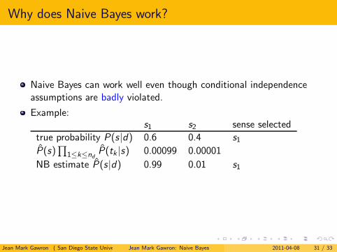
Naive Bayes can work well even though conditional independenceassumptions are badly violated.
Example:s1 s2 sense selected
true probability P(s|d) 0.6 0.4 s1
P̂(s)∏
1≤k≤ndP̂(tk |s) 0.00099 0.00001
NB estimate P̂(s|d) 0.99 0.01 s1
Jean Mark Gawron ( San Diego State University )Jean Mark Gawron: Naive Bayes 2011-04-08 31 / 33

Illustration
Suppose the featues are NOT independent, causing, say,underestimation P(s2 | d) = 0.01).
P(s2|tk , tj) > P̂(s1|tk)P̂(s2|tj)
Then P(s1|tk , tj) will be overestimated (0.99):
P(s1|tk , tj) < P̂(s1|tk)P̂(s1|tj)
As long as NB overestimates the larger prob, it will still make correctclassification decisions. Even if NB overestimates the smaller prob,the decision might still be right.
Classification is about predicting the correct class and not aboutaccurately estimating probabilities.
Correct estimation ⇒ accurate prediction.
But not vice versa!
Jean Mark Gawron ( San Diego State University )Jean Mark Gawron: Naive Bayes 2011-04-08 32 / 33

Naive Bayes is not so naive
Naive Bayes has won some bakeoffs (e.g., KDD-CUP 97)
More robust to nonrelevant features than some more complex learningmethods
More robust to concept drift (changing of definition of class overtime) than some more complex learning methods
Better than methods like decision trees when we have many equallyimportant features
A good dependable baseline for text classification (but not the best)
Optimal if independence assumptions hold (never true for text, buttrue for some domains)
Very fast
Low storage requirements
Jean Mark Gawron ( San Diego State University )Jean Mark Gawron: Naive Bayes 2011-04-08 33 / 33