Introduction to Computational Fluid Dynamics:

Governing Equations, Turbulence Modeling Introduction and

Finite Volume Discretization Basics.

Joel Guerrero

February 13, 2014

Contents

1 Notation and Mathematical Preliminaries 2

2 Governing Equations of Fluid Dynamics 72.1 Simplification of the Navier-Stokes System of Equations: Incompressible Viscous

Flow Case . . . . . . . . . . . . . . . . . . . . . . . . . . . . . . . . . . . . . . . . 11

3 Turbulence Modeling 133.1 Reynolds Averaging . . . . . . . . . . . . . . . . . . . . . . . . . . . . . . . . . . 143.2 Incompressible Reynolds Averaged Navier-Stokes Equations . . . . . . . . . . . . 163.3 Boussinesq Approximation . . . . . . . . . . . . . . . . . . . . . . . . . . . . . . . 173.4 Two-Equations Models. The κ− ω Model . . . . . . . . . . . . . . . . . . . . . . 18

4 Finite Volume Method Discretization 204.1 Discretization of the Solution Domain . . . . . . . . . . . . . . . . . . . . . . . . 214.2 Discretization of the Transport Equation . . . . . . . . . . . . . . . . . . . . . . . 22

4.2.1 Approximation of Surface Integrals and Volume Integrals . . . . . . . . . 234.2.2 Convective Term Spatial Discretization . . . . . . . . . . . . . . . . . . . 254.2.3 Diffusion Term Spatial Discretization . . . . . . . . . . . . . . . . . . . . . 274.2.4 Evaluation of Gradient Terms . . . . . . . . . . . . . . . . . . . . . . . . . 314.2.5 Source Terms Spatial Discretization . . . . . . . . . . . . . . . . . . . . . 324.2.6 Temporal Discretization . . . . . . . . . . . . . . . . . . . . . . . . . . . . 334.2.7 System of Algebraic Equations . . . . . . . . . . . . . . . . . . . . . . . . 354.2.8 Boundary Conditions and Initial Conditions . . . . . . . . . . . . . . . . . 35

4.3 Discretization Errors . . . . . . . . . . . . . . . . . . . . . . . . . . . . . . . . . . 364.3.1 Taylor Series Expansions . . . . . . . . . . . . . . . . . . . . . . . . . . . 364.3.2 Accuracy of the Upwind Scheme and Central Differencing Scheme . . . . 394.3.3 Mean Value Approximation . . . . . . . . . . . . . . . . . . . . . . . . . . 404.3.4 Gradient Approximation . . . . . . . . . . . . . . . . . . . . . . . . . . . . 414.3.5 Spatial and Temporal Linear Variation . . . . . . . . . . . . . . . . . . . . 424.3.6 Mesh Induced Errors . . . . . . . . . . . . . . . . . . . . . . . . . . . . . . 424.3.7 Mesh Spacing . . . . . . . . . . . . . . . . . . . . . . . . . . . . . . . . . . 46

5 The Finite Volume Method for Diffusion and Convection-Diffusion Problems 505.1 Steady One-Dimensional Diffusion . . . . . . . . . . . . . . . . . . . . . . . . . . 505.2 Steady One-Dimensional Convection-Diffusion . . . . . . . . . . . . . . . . . . . . 505.3 Steady one-dimensional convection-diffusion working example . . . . . . . . . . . 525.4 Unsteady One-Dimensional Diffusion . . . . . . . . . . . . . . . . . . . . . . . . . 555.5 Unsteady One-Dimensional Convection-Diffusion . . . . . . . . . . . . . . . . . . 55

6 Finite Volume Method Algorithms for Pressure-Velocity Coupling 56

1

Chapter 1

Notation and MathematicalPreliminaries

When presenting the fluid flow equations, as well as throughout this manuscript, we make useof the following vector/tensor notation and mathematical operators.

From now on we are going to refer to a zero rank tensor as a scalar. A first rank tensor willbe referred as a vector. And a second rank tensor will associated to a tensor. Vectors willbe denoted by minuscule bold letters, whereas tensors by majuscule bold letters or bold greeksymbols. Scalars will be represented by normal letters or normal greek symbols.

Hereafter, the vector is almost always a column vector and a row vector is expressed as atranspose of a column vector indicated by the superscript T. Vectors a = a1i + a2j + a3k andb = b1i + b2j + b3k are expressed as follows

a =

a1

a2

a3

, b =

b1b2b3

,the transpose of the column vectors a and b are represented as follows

aT = [a1, a2, a3] , bT = [b1, b2, b3] ,

The magnitude of a vector a is defined as |a| = (a · a)12 = (a1

2 + a22 + a3

2)12 .

A tensor is represented as follows

A =

A11 A12 A13

A21 A22 A23

A31 A32 A33

, AT =

A11 A21 A31

A12 A22 A32

A13 A23 A33

.If A = AT, the tensor is said to be symmetric, that is, its components are symmetric about thediagonal.

The dot product of two vectors a and b (also known as scalar product of two vectors), yields toa scalar quantity and is given by

aT · b = a · b =[a1, a2, a3

] b1b2b3

= a1b1 + a2b2 + a3b3.

2

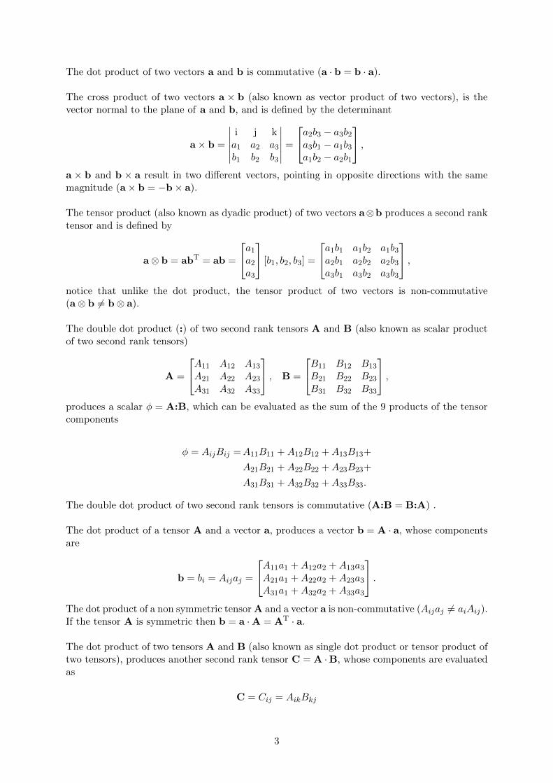
The dot product of two vectors a and b is commutative (a · b = b · a).

The cross product of two vectors a × b (also known as vector product of two vectors), is thevector normal to the plane of a and b, and is defined by the determinant

a× b =

∣∣∣∣∣∣i j ka1 a2 a3

b1 b2 b3

∣∣∣∣∣∣ =

a2b3 − a3b2a3b1 − a1b3a1b2 − a2b1

,a × b and b × a result in two different vectors, pointing in opposite directions with the samemagnitude (a× b = −b× a).

The tensor product (also known as dyadic product) of two vectors a⊗b produces a second ranktensor and is defined by

a⊗ b = abT = ab =

a1

a2

a3

[b1, b2, b3] =

a1b1 a1b2 a1b3a2b1 a2b2 a2b3a3b1 a3b2 a3b3

,notice that unlike the dot product, the tensor product of two vectors is non-commutative(a⊗ b 6= b⊗ a).

The double dot product (:) of two second rank tensors A and B (also known as scalar productof two second rank tensors)

A =

A11 A12 A13

A21 A22 A23

A31 A32 A33

, B =

B11 B12 B13

B21 B22 B23

B31 B32 B33

,produces a scalar φ = A:B, which can be evaluated as the sum of the 9 products of the tensorcomponents

φ = AijBij =A11B11 +A12B12 +A13B13+

A21B21 +A22B22 +A23B23+

A31B31 +A32B32 +A33B33.

The double dot product of two second rank tensors is commutative (A:B = B:A) .

The dot product of a tensor A and a vector a, produces a vector b = A · a, whose componentsare

b = bi = Aijaj =

A11a1 +A12a2 +A13a3

A21a1 +A22a2 +A23a3

A31a1 +A32a2 +A33a3

.The dot product of a non symmetric tensor A and a vector a is non-commutative (Aijaj 6= aiAij).If the tensor A is symmetric then b = a ·A = AT · a.

The dot product of two tensors A and B (also known as single dot product or tensor product oftwo tensors), produces another second rank tensor C = A ·B, whose components are evaluatedas

C = Cij = AikBkj

3

The dot product of two tensors is non-commutative (A ·B 6= B ·A).

Note that our definitions of the tensor-vector dot product and tensor-tensor dot-product areconsistent with the ordinary rules of matrix algebra.

The trace of a tensor A is a scalar, evaluated by summing its diagonal components

tr A = Atr = A11 +A22 +A33.

The gradient operator ∇ (read as nabla) in Cartesian coordinates is defined by

∇ =∂

∂xi +

∂

∂yj +

∂

∂zk =

(∂

∂x,∂

∂y,∂

∂z

)T

.

The gradient operator ∇ when applied to a scalar quantity φ(x, y, z) (where x,y, z are the spatialcoordinates), yields to a vector defined by

∇φ =

(∂φ

∂x,∂φ

∂y,∂φ

∂z

)T

.

The notation grad for ∇ may be also used as the gradient operator, so that, grad φ ≡ ∇φ. Thegradient of a vector a produces a second rank tensor

grada = ∇a =

∂a1

∂x

∂a1

∂y

∂a1

∂z∂a2

∂x

∂a2

∂y

∂a2

∂z∂a3

∂x

∂a3

∂y

∂a3

∂z

.The gradient can operate on any tensor field to produce a tensor field that is one rank higher.

The dot product of vector a and the operator ∇ is called the divergence (div) of the vector field;the output of this operator is a scalar and is defined as

div a = ∇ · a =∂a1

∂x+∂a2

∂y+∂a3

∂z.

The divergence of a tensor A, div A or ∇ ·A, yields to a vector and is defined as

divA = ∇ ·A =

∂A11

∂x+∂A12

∂y+∂A13

∂z∂A21

∂x+∂A22

∂y+∂A23

∂z∂A31

∂x+∂A32

∂y+∂A33

∂z

.The divergence can operate on any tensor field of rank 1 and above to produce a tensor that isone rank lower.

The curl operator of a vector a produces another vector. This operator is defined by

curl a = ∇× a =

∣∣∣∣∣∣∣∣i j k∂

∂x

∂

∂y

∂

∂za1 a2 a3

∣∣∣∣∣∣∣∣ =

(∂a3

∂y− ∂a2

∂z,∂a1

∂z− ∂a3

∂x,∂a2

∂x− ∂a1

∂y

)T

.

The divergence of the gradient is called the Laplacian operator and is denoted by ∆. TheLaplacian of a scalar φ(x, y, z) yields to another scalar field and is defined as

4

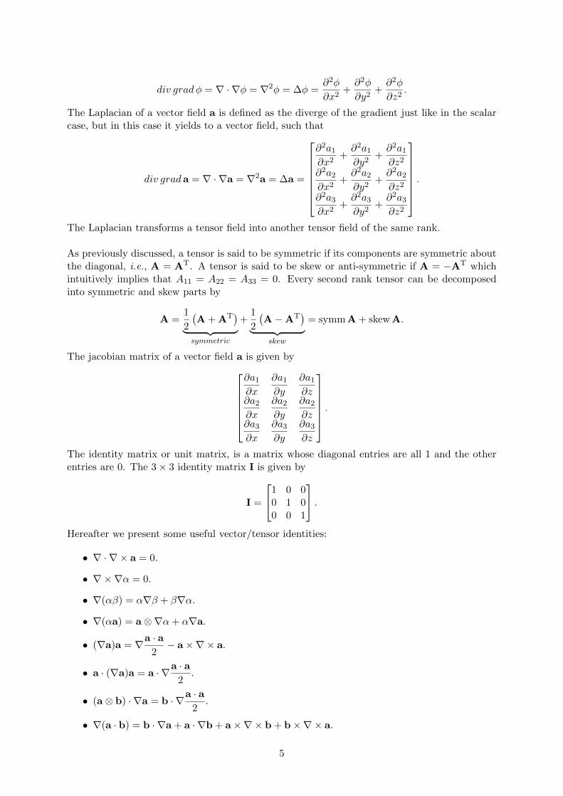
div grad φ = ∇ · ∇φ = ∇2φ = ∆φ =∂2φ

∂x2+∂2φ

∂y2+∂2φ

∂z2.

The Laplacian of a vector field a is defined as the diverge of the gradient just like in the scalarcase, but in this case it yields to a vector field, such that

div grada = ∇ · ∇a = ∇2a = ∆a =

∂2a1

∂x2+∂2a1

∂y2+∂2a1

∂z2

∂2a2

∂x2+∂2a2

∂y2+∂2a2

∂z2

∂2a3

∂x2+∂2a3

∂y2+∂2a3

∂z2

.

The Laplacian transforms a tensor field into another tensor field of the same rank.

As previously discussed, a tensor is said to be symmetric if its components are symmetric aboutthe diagonal, i.e., A = AT. A tensor is said to be skew or anti-symmetric if A = −AT whichintuitively implies that A11 = A22 = A33 = 0. Every second rank tensor can be decomposedinto symmetric and skew parts by

A =1

2

(A + AT

)︸ ︷︷ ︸symmetric

+1

2

(A−AT

)︸ ︷︷ ︸

skew

= symm A + skew A.

The jacobian matrix of a vector field a is given by∂a1

∂x

∂a1

∂y

∂a1

∂z∂a2

∂x

∂a2

∂y

∂a2

∂z∂a3

∂x

∂a3

∂y

∂a3

∂z

.The identity matrix or unit matrix, is a matrix whose diagonal entries are all 1 and the otherentries are 0. The 3× 3 identity matrix I is given by

I =

1 0 00 1 00 0 1

.Hereafter we present some useful vector/tensor identities:

• ∇ · ∇ × a = 0.

• ∇ ×∇α = 0.

• ∇(αβ) = α∇β + β∇α.

• ∇(αa) = a⊗∇α+ α∇a.

• (∇a)a = ∇a · a2− a×∇× a.

• a · (∇a)a = a · ∇a · a2.

• (a⊗ b) · ∇a = b · ∇a · a2.

• ∇(a · b) = b · ∇a + a · ∇b + a×∇× b + b×∇× a.

5

• ∇ · (αa) = α∇ · a + a · ∇α.

• ∇ · ∇a = ∇(∇ · a)−∇× (∇× a).

• ∇ · (a× b) = b · ∇ × a− a · ∇ × b.

• ∇ · (a⊗ b) = b · ∇a + a∇ · b.

• a · ∇ · (b⊗ c) = (a · b)∇ · c + (a⊗ b) · ∇b.

• ∇ · (αA) = A∇α+ α∇ ·A.

• ∇ · (Ab) = (∇ ·AT) · b + AT · ∇b.

• ∇ × (αa) = α∇× a +∇α× a.

• ∇ × (a× b) = a∇ · b + b · ∇a− (∇ · a)b− a · ∇b.

• a · (Ab) = A · (a⊗ b).

• a · (Ab) = (Aa) · b if A is symmetric.

• ab:A = a · (b ·A)

• A:ab = (A · a) · b

where α and β are scalars; a, b and c are vectors; and A is a tensor.

6

Chapter 2

Governing Equations of FluidDynamics

The starting point of any numerical simulation are the governing equations of the physics of theproblem to be solved. Hereafter, we present the governing equations of fluid dynamics and theirsimplification for the case of an incompressible viscous flow.

The equations governing the motion of a fluid can be derived from the statements of the conser-vation of mass, momentum, and energy [1, 2, 3]. In the most general form, the fluid motion isgoverned by the time-dependent three-dimensional compressible Navier-Stokes system of equa-tions. For a viscous Newtonian, isotropic fluid in the absence of external forces, mass diffusion,finite-rate chemical reactions, and external heat addition; the conservation form of the Navier-Stokes system of equations in compact differential form and in primitive variable formulation(ρ, u, v, w, et) can be written as

∂ρ

∂t+∇ · (ρu) = 0,

∂ (ρu)

∂t+∇ · (ρuu) = −∇p+∇ · τ ,

∂ (ρet)

∂t+∇ · (ρetu) = ∇ · q −∇ · (pu) + τ :∇u,

(2.0.1)

where τ is the viscous stress tensor and is given by

τ =

τxx τxy τxzτyx τyy τyzτzx τzy τzz

. (2.0.2)

For the sake of completeness, let us recall that in the conservation form (or divergence form)[4], the momentum equation can be written as

∂ (ρu)

∂t+∇ · (ρuu) = −∇p+∇ · τ , (2.0.3)

where the tensor product of the vectors uu in eq. 2.0.3 is equal to

uu =

uvw

[u v w]

=

u2 uv uwvu v2 vwwu wv w2

. (2.0.4)

Let us recall the following identity

7

∇ · (uu) = u · ∇u + u(∇ · u), (2.0.5)

and from the divergence-free constraint (∇ · u = 0) it follows that u(∇ · u) is zero, therefore∇ · (uu) = u · ∇u. Henceforth, the conservation form of the momentum equation eq. 2.0.3 isequivalent to

ρ

(∂ (u)

∂t+ u · ∇ (u)

)= −∇p+∇ · τ ,

which is the non-conservation form or advective/convective form of the momentum equation.

The set of equations 2.0.1 can be rewritten in vector form as follows

∂q

∂t+∂ei∂x

+∂fi∂y

+∂gi

∂z=∂ev∂x

+∂fv∂y

+∂gv

∂z, (2.0.6)

where q is the vector of the conserved flow variables given by

q =

ρρuρvρwρet

, (2.0.7)

and ei, fi and gi are the vectors containing the inviscid fluxes (or convective fluxes) in the x, yand z directions and are given by

ei =

ρu

ρu2 + pρuvρuw

(ρet + p)u

, fi =

ρvρvu

ρv2 + pρvw

(ρet + p) v

, gi =

ρwρwuρwv

ρw2 + p(ρet + p)w

, (2.0.8)

where u is the velocity vector containing the u, v and w velocity components in the x, y andz directions and p, ρ and et are the pressure, density and total energy per unit mass respectively.

The vectors ev, fv and gv contain the viscous fluxes (or diffusive fluxes) in the x, y and zdirections and are defined as follows

ev =

0τxxτxyτxz

uτxx + vτxy + wτxz − qx

,

fv =

0τyxτyyτyz

uτyx + vτyy + wτyz − qy

,

gv =

0τzxτzyτzz

uτzx + vτzy + wτzz − qz

,

(2.0.9)

8

where the heat fluxes qx, qy and qz are given by the Fourier’s law of heat conduction as follows

qx = −k ∂T∂x

,

qy = −k ∂T∂y

,

qz = −k ∂T∂z

,

(2.0.10)

and the viscous stresses τxx, τyy, τzz, τxy, τyx, τxz, τzx, τyz and τzy, are given by the followingrelationships

τxx =2

3µ

(2∂u

∂x− ∂v

∂y− ∂w

∂z

),

τyy =2

3µ

(2∂v

∂y− ∂u

∂x− ∂w

∂z

),

τzz =2

3µ

(2∂w

∂z− ∂u

∂x− ∂v

∂y

),

τxy = τyx = µ

(∂u

∂y+∂v

∂x

),

τxz = τzx = µ

(∂u

∂z+∂w

∂x

),

τyz = τzy = µ

(∂v

∂z+∂w

∂y

),

(2.0.11)

In equations 2.0.9-2.0.11, T is the temperature, k is the thermal conductivity and µ is the laminarviscosity. In order to derive the viscous stresses in eq. 2.0.11 the Stokes’s hypothesis was used [5].

Examining closely equations 2.0.6-2.0.11 and counting the number of equations and unknowns,we clearly see that we have five equations in terms of seven unknown flow field variables u, v,w, ρ, p, T , and et. It is obvious that two additional equations are required to close the system.These two additional equations can be obtained by determining relationships that exist betweenthe thermodynamic variables (p, ρ, T, ei) through the assumption of thermodynamic equilibrium.Relations of this type are known as equations of state, and they provide a mathematical rela-tionship between two or more state functions (thermodynamic variables). Choosing the specificinternal energy ei and the density ρ as the two independent thermodynamic variables, thenequations of state of the form

p = p (ei, ρ) , T = T (ei, ρ) , (2.0.12)

are required. For most problems in aerodynamics and gasdynamics, it is generally reasonableto assume that the gas behaves as a perfect gas (a perfect gas is defined as a gas whose inter-molecular forces are negligible), i.e.,

p = ρRgT, (2.0.13)

where Rg is the specific gas constant and is equal to 287 m2

s2Kfor air. Assuming also that the

working gas behaves as a calorically perfect gas (a calorically perfect gas is defined as a perfectgas with constant specific heats), then the following relations hold

ei = cvT, h = cpT, γ =cpcv, cv =

Rgγ − 1

, cp =γRgγ − 1

, (2.0.14)

9

where γ is the ratio of specific heats and is equal to 1.4 for air, cv the specific heat at constantvolume, cp the specific heat at constant pressure and h is the enthalpy. By using eq. 2.0.13 andeq. 2.0.14, we obtain the following relations for pressure p and temperature T in the form of eq.2.0.12

p = (γ − 1) ρei, T =p

ρRg=

(γ − 1) eiRg

, (2.0.15)

where the specific internal energy per unit mass ei = p/(γ − 1)ρ is related to the total energyper unit mass et by the following relationship,

et = ei +1

2

(u2 + v2 + w2

). (2.0.16)

In our discussion, it is also necessary to relate the transport properties (µ, k) to the thermody-namic variables. Then, the laminar viscosity µ is computed using Sutherland’s formula

µ =C1T

32

(T + C2), (2.0.17)

where for the case of the air, the constants are C1 = 1.458× 10−6 kg

ms√K

and C2 = 110.4K.

The thermal conductivity, k, of the fluid is determined from the Prandtl number (Pr = 0.72 for air)which in general is assumed to be constant and is equal to

k =cpµ

Pr, (2.0.18)

where cp and µ are given by equations eq. 2.0.14 and eq. 2.0.17 respectively.

When dealing with high speed compressible flows, it is also useful to introduce the Mach number.The mach number is a non dimensional parameter that measures the speed of the gas motionin relation to the speed of sound a,

a =

[(∂p

∂ρ

)S

] 12

=

√γp

ρ=√γRgT . (2.0.19)

Then the Mach number M∞ is given by,

M∞ =U∞a

=U∞√γ(p/ρ)

=U∞√γRgT

(2.0.20)

Another useful non dimensional quantity is the Reynold’s number, this quantity represents theratio of inertia forces to viscous forces and is given by,

Re =ρ∞U∞L

µ∞, (2.0.21)

where the subscript ∞ denotes freestream conditions, L is a reference length (such as the chordof an airfoil or the length of a vehicle), and µ∞ is computed using the freestream temperatureT∞ according to eq 2.0.17.

The first row in eq. 2.0.6 corresponds to the continuity equation. Likewise, the second, thirdand fourth rows are the momentum equations, while the fifth row is the energy equation in termsof total energy per unit mass.

The Navier-Stokes system of equations 2.0.6-2.0.9, is a coupled system of nonlinear partial differ-ential equations (PDE), and hence is very difficult to solve analytically. In fact, to the date there

10

is no general closed-form solution to this system of equations; hence we look for an approximatesolution of this system of equation in a given domain D with prescribed boundary conditions∂D and given initial conditions Dq.

If in eq. 2.0.6 we set the viscous fluxes ev = 0, fv = 0 and gv = 0, we get the Euler system ofequations, which governs inviscid fluid flow. The Euler system of equations is a set of hyperbolicequations while the Navier-Stokes system of equations is a mixed set of hyperbolic (in the inviscidregion) and parabolic (in the viscous region) equations. Therefore, time marching algorithmsare used to advance the solution in time using discrete time steps.

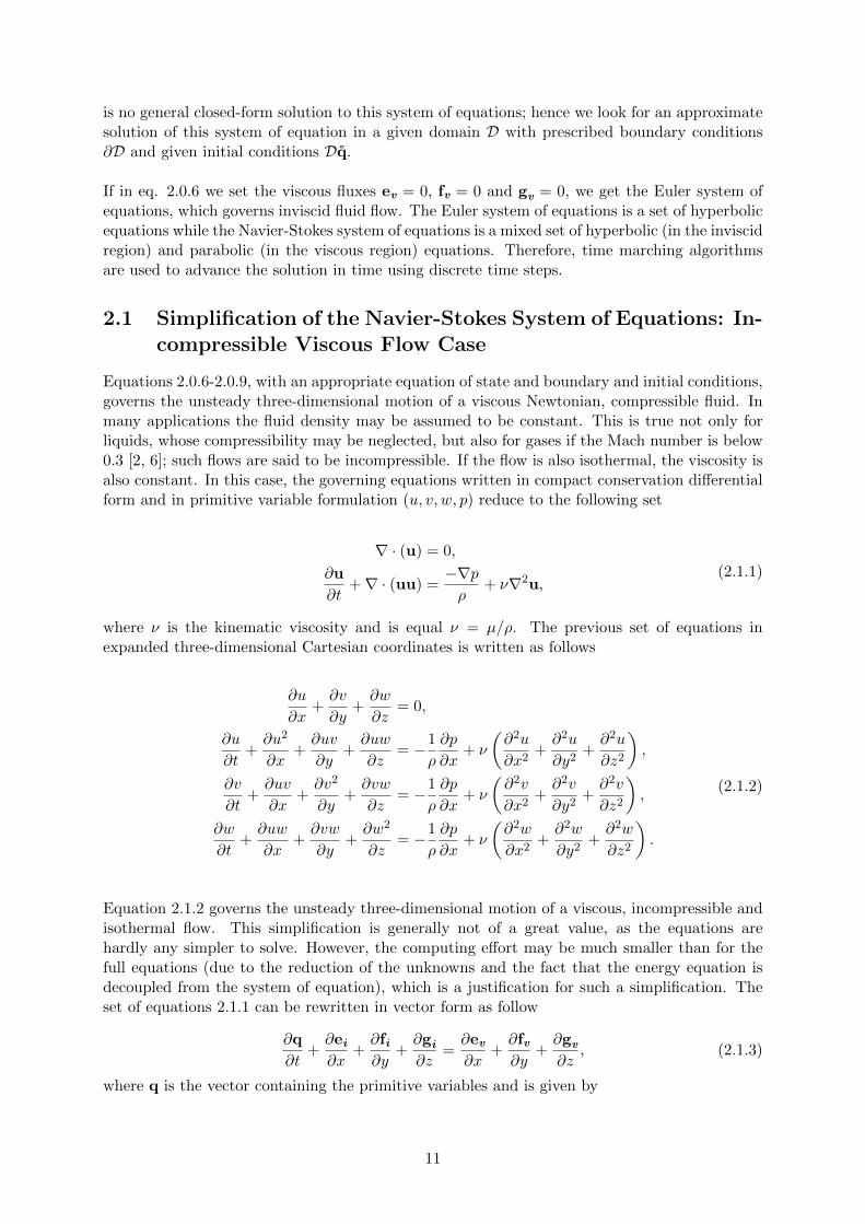
2.1 Simplification of the Navier-Stokes System of Equations: In-compressible Viscous Flow Case

Equations 2.0.6-2.0.9, with an appropriate equation of state and boundary and initial conditions,governs the unsteady three-dimensional motion of a viscous Newtonian, compressible fluid. Inmany applications the fluid density may be assumed to be constant. This is true not only forliquids, whose compressibility may be neglected, but also for gases if the Mach number is below0.3 [2, 6]; such flows are said to be incompressible. If the flow is also isothermal, the viscosity isalso constant. In this case, the governing equations written in compact conservation differentialform and in primitive variable formulation (u, v, w, p) reduce to the following set

∇ · (u) = 0,

∂u

∂t+∇ · (uu) =

−∇pρ

+ ν∇2u,(2.1.1)

where ν is the kinematic viscosity and is equal ν = µ/ρ. The previous set of equations inexpanded three-dimensional Cartesian coordinates is written as follows

∂u

∂x+∂v

∂y+∂w

∂z= 0,

∂u

∂t+∂u2

∂x+∂uv

∂y+∂uw

∂z= −1

ρ

∂p

∂x+ ν

(∂2u

∂x2+∂2u

∂y2+∂2u

∂z2

),

∂v

∂t+∂uv

∂x+∂v2

∂y+∂vw

∂z= −1

ρ

∂p

∂x+ ν

(∂2v

∂x2+∂2v

∂y2+∂2v

∂z2

),

∂w

∂t+∂uw

∂x+∂vw

∂y+∂w2

∂z= −1

ρ

∂p

∂x+ ν

(∂2w

∂x2+∂2w

∂y2+∂2w

∂z2

).

(2.1.2)

Equation 2.1.2 governs the unsteady three-dimensional motion of a viscous, incompressible andisothermal flow. This simplification is generally not of a great value, as the equations arehardly any simpler to solve. However, the computing effort may be much smaller than for thefull equations (due to the reduction of the unknowns and the fact that the energy equation isdecoupled from the system of equation), which is a justification for such a simplification. Theset of equations 2.1.1 can be rewritten in vector form as follow

∂q

∂t+∂ei∂x

+∂fi∂y

+∂gi

∂z=∂ev∂x

+∂fv∂y

+∂gv

∂z, (2.1.3)

where q is the vector containing the primitive variables and is given by

11

q =

0uvw

, (2.1.4)

and ei, fi and gi are the vectors containing the inviscid fluxes (or convective fluxes) in the x, yand z directions and are given by

ei =

u

u2 + puvuw

, fi =

vvu

v2 + pvw

, gi =

wwuwv

w2 + p

. (2.1.5)

The viscous fluxes (or diffusive fluxes) in the x, y and z directions, ev, fv and gv respectively,are defined as follows

ev =

0τxxτxyτxz

, fv =

0τyxτyyτyz

, gv =

0τzxτzyτzz

. (2.1.6)

Since we made the assumptions of an incompressible flow, appropriate expressions for shearstresses must be used, these expressions are given as follows

τxx = 2µ∂u

∂x,

τyy = 2µ∂v

∂y,

τzz = 2µ∂w

∂z,

τxy = τyx = µ

(∂u

∂y+∂v

∂x

),

τxz = τzx = µ

(∂w

∂x+∂u

∂z

),

τyz = τzy = µ

(∂w

∂y+∂v

∂z

),

(2.1.7)

where we used Stokes’s hypothesis [5] in order to derive the viscous stresses in eq. 2.1.7.

Equation 2.1.7 can be written in compact vector form as τ = 2µD, where D = 12

[∇u +∇uT

]is the symmetric tensor of the velocity gradient tensor ∇u = [D + S], and where D representsthe strain-rate tensor and S represents the spin tensor (vorticity). The skew or anti-symmetricpart of the velocity gradient tensor is given by S = 1

2

[∇u−∇uT

].

Equations 2.1.3-2.1.6, are the governing equations of an incompressible, isothermal, viscous flowwritten in conservation form. Hence, we look for an approximate solution of this set of equationsin a given domain D with prescribed boundary conditions ∂D and given initial conditions Dq.

12

Chapter 3

Turbulence Modeling

All flows encountered in engineering applications, from simple ones to complex three-dimensionalones, become unstable above a certain Reynolds number (Re = UL/ν where U and L are char-acteristic velocity and length scales of the mean flow and ν is the kinematic viscosity). At lowReynolds numbers flows are laminar, but as we increase the Reynolds number, flows are observedto become turbulent. Turbulent flows are characterize by a chaotic and random state of motionin which the velocity and pressure change continuously on a broad range of time and lengthscales (from the smallest turbulent eddies characterized by Kolmogorov micro-scales, to the flowfeatures comparable with the size of the geometry).

There are several possible approaches for the numerical simulation of turbulent flows. The firstand most intuitive one, is by directly numerically solving the governing equations over the wholerange of turbulent scales (temporal and spatial). This deterministic approach is referred as Di-rect Numerical Simulation (DNS) [15, 16, 17, 10, 22, 23]. In DNS, a fine enough mesh and smallenough time-step size must be used so that all of the turbulent scales are resolved. Althoughsome simple problems have been solved using DNS, it is not possible to tackle industrial prob-lems due to the prohibitive computer cost imposed by the mesh and time-step requirements.Hence, this approach is mainly used for benchmarking, research and academic applications.

Another approach used to model turbulent flows is Large Eddy Simulation (LES) [18, 19, 15,22, 23]. Here, large scale turbulent structures are directly simulated whereas the small turbulentscales are filtered out and modeled by turbulence models called subgrid scale models. Accordingto turbulence theory, small scale eddies are more uniform and have more or less common char-acteristics; therefore, modeling small scale turbulence appears more appropriate, rather thanresolving it. The computational cost of LES is less than that of DNS, since the small scaleturbulence is now modeled, hence the grid spacing is much larger than the Kolmogorov lengthscale. In LES, as the mesh gets finer, the number of scales that require modeling becomessmaller, thus approaching DNS. Thanks to the advances in computing hardware and parallelalgorithms, the use of LES for industrial problems is becoming practical.

Today’s workhorse for industrial and research turbulence modeling applications is the ReynoldsAveraged Navier-Stokes (RANS) approach [20, 21, 22, 10, 12, 23]. In this approach, the RANSequations are derived by decomposing the flow variables of the governing equations into time-mean (obtained over an appropriate time interval) and fluctuating part, and then time averagingthe entire equations. Time averaging the governing equations gives rise to new terms, these newquantities must be related to the mean flow variables through turbulence models. This pro-cess introduces further assumptions and approximations. The turbulence models are primarilydeveloped based on experimental data obtained from relatively simple flows under controlledconditions. This in turn limits the range of applicability of the turbulence models. That is, no

13

single RANS turbulence model is capable of providing accurate solutions over a wide range offlow conditions and geometries.

Two types of averaging are presently used, the classical Reynolds averaging which gives riseto the RANS equations and the mass-weighted averaging or Favre averaging which is used toderive the Favre-Averaged Navier-Stokes equations (FANS) for compressible flows applications.In both statistical approaches, all the turbulent scales are modeled, hence mesh and time-steprequirements are not as restrictive as in LES or DNS. Hereafter, we limit our discussion toReynolds averaging.

3.1 Reynolds Averaging

The starting point for deriving the RANS equations is the Reynolds decomposition [20, 3, 22,10, 12, 23] of the flow variables of the governing equations. This decomposition is accomplishedby representing the instantaneous flow quantity φ by the sum of a mean value part (denoted bya bar over the variable, as in φ) and a time-dependent fluctuating part (denoted by a prime, asin φ′). This concept is illustrated in figure 3.1 and is mathematically expressed as follows,

φ(x, t) = φ(x)︸︷︷︸mean value

+ φ′(x, t)︸ ︷︷ ︸fluctuating part

. (3.1.1)

Figure 3.1: Time averaging for a statistically steady turbulent flow (left) and time averaging for anunsteady turbulent flow (right).

Hereafter, x is the vector containing the Cartesian coordinates x, y, and z in N = 3 (whereN is equal to the number of spatial dimensions). A key observation in eq. 3.1.1 is that φ isindependent of time, implying that any equation deriving for computing this quantity must besteady state.

In eq. 3.1.1, the mean value φ is obtained by an averaging procedure. There are three differentforms of the Reynolds averaging:

1. Time averaging: appropriate for stationary turbulence, i.e., statically steady turbulenceor a turbulent flow that, on average, does not vary with time.

φ(x) = limT→+∞

1

T

∫ t+T

tφ(x, t) dt, (3.1.2)

14

here t is the time and T is the averaging interval. This interval must be large comparedto the typical time scales of the fluctuations; thus, we are interested in the limit T →∞.As a consequence, φ does not vary in time, but only in space.

2. Spatial averaging: appropriate for homogeneous turbulence.

φ(t) = limCV→∞

1

CV

∫CVφ(x, t) dCV, (3.1.3)

with CV being a control volume. In this case, φ is uniform in space, but it is allowed tovary in time.

3. Ensemble averaging: appropriate for unsteady turbulence.

φ(x, t) = limN→∞

1

N

N∑i=1

φ(x, t), (3.1.4)

where N , is the number of experiments of the ensemble and must be large enough toeliminate the effects of fluctuations. This type of averaging can be applied to any flow(steady or unsteady). Here, the mean value φ is a function of both time and space (asillustrated in figure 3.1).

We use the term Reynolds averaging to refer to any of these averaging processes, applying any ofthem to the governing equations yields to the Reynolds-Averaged Navier-Stokes (RANS) equa-tions. In cases where the turbulent flow is both stationary and homogeneous, all three averagingare equivalent. This is called the ergodic hypothesis.

If the mean flow φ varies slowly in time, we should use an unsteady approach (URANS); then,equations eq. 3.1.1 and eq. 3.1.2 can be modified as

φ(x, t) = φ(x, t) + φ′(x, t), (3.1.5)

and

φ(x, t) =1

T

∫ t+T

tφ(x, t)dt, T1 << T << T2, (3.1.6)

where T1 and T2 are the characteristics time scales of the fluctuations and the slow variationsin the flow, respectively (as illustrated in figure 3.1). In eq. 3.1.6 the time scales should differby several order of magnitude, but in engineering applications very few unsteady flows satisfythis condition. In general, the mean and fluctuating components are correlated, i.e., the timeaverage of their product is non-vanishing. For such problems, ensemble averaging is necessary.An alternative approach to URANS is LES, which is out of the scope of this discussion but theinterested reader should refer to references [18, 19, 15, 22, 23].

Before deriving the RANS equations, we recall the following averaging rules,

15

φ′ = 0,

φ = φ,

φ = φ+ φ′ = φ,

∂φ

∂x=∂φ

∂x,

φ+ ϕ = φ+ ϕ ,

φϕ = φϕ = φϕ,

φϕ = φϕ,

φϕ′ = φϕ′ = 0,

φϕ = (φ+ φ′)(ϕ+ ϕ′)

= φϕ+ φϕ′ + ϕφ′ + φ′ϕ′

= φϕ+ φϕ′ + ϕφ′ + φ′ϕ′

= φϕ+ φ′ϕ′,

φ′2 6= 0,

φ′ϕ′ 6= 0.

(3.1.7)

3.2 Incompressible Reynolds Averaged Navier-Stokes Equations

Let us recall the Reynolds decomposition for the flow variables of the incompressible Navier-Stokes equations eq. 2.1.1,

u(x, t) = u(x) + u′(x, t),

p(x, t) = p(x) + p′(x, t),(3.2.1)

we now substitute eq. 3.2.1 into the incompressible Navier-Stokes equations eq. 2.1.1 and weobtain for the continuity equation

∇ · (u) = ∇ ·(u + u′

)= ∇ · (u) +∇ ·

(u′)

= 0. (3.2.2)

Then, time averaging this equation results in

∇ · (u) +∇ ·(u′)

= 0, (3.2.3)

and using the averaging rules stated in eq. 3.1.7, it follows that

∇ · (u) = 0. (3.2.4)

We next consider the momentum equation of the incompressible Navier-Stokes equations eq.2.1.1. We begin by substituting eq. 3.2.1 into eq. 2.1.1 in order to obtain,

∂ (u + u′)

∂t+∇ ·

((u + u′

) (u + u′

))=−∇ (p+ p′)

ρ+ ν∇2

(u + u′

), (3.2.5)

by time averaging eq. 3.2.5, expanding and applying the rules set in eq. 3.1.7, we obtain

∂u

∂t+∇ ·

(uu + u′u′

)=−∇pρ

+ ν∇2u. (3.2.6)

16

Grouping equations 3.2.4 and 3.2.6, we obtain the following set of equations,

∇ · (u) = 0,

∂u

∂t+∇ · (uu) =

−∇pρ

+ ν∇2u− 1

ρ∇ · τR.

(3.2.7)

The set of equations eq. 3.2.7 are the incompressible Reynolds-Averaged Navier-Stokes (RANS)equations. Notice that in eq. 3.2.7 we have retained the term ∂u/∂t, despite the fact thatu is independent of time for statistically steady turbulence, hence this expression is equal tozero when time average. In practice, in all modern formulations of the RANS equations thetime derivative term is included. In references [20, 22, 3, 16, 25], a few arguments justifyingthe retention of this term are discussed. For not statistically stationary turbulence or unsteadyturbulence, a time-dependent RANS or unsteady RANS (URANS) approach is required, anURANS computation simply requires retaining the time derivative term ∂u/∂t in the computa-tion. For unsteady turbulence, ensemble average is recommended and often necessary.

The incompressible Reynolds-Averaged Navier-Stokes (RANS) equations eq. 3.2.7 are identicalto the incompressible Navier-Stokes equations eq. 2.1.1 with the exception of the additional termτR = −ρ

(u′u′

), where τR is the so-called Reynolds-stress tensor (notice that by doing a check

of dimensions, it will show that τR it is not actually a stress; it must be multiplied by the densityρ, as it is done consistently in this manuscript, in order to have dimensions corresponding to thestresses. On the other hand, since we are assuming that the flow is incompressible, that is, ρ isconstant, we might set the density equal to unity, thus obtaining implicit dimensional correctness.Moreover, because we typically use kinematic viscosity ν, there is an implied division by ρ inany case). The Reynolds-stress tensor represents the transfer of momentum due to turbulentfluctuations. In 3D, the Reynolds-stress tensor τR consists of nine components

τR = −ρ(u′u′

)= −

ρu′u′ ρu′v′ ρu′w′

ρv′u′ ρv′v′ ρv′w′

ρw′u′ ρw′v′ ρw′w′

. (3.2.8)

However, since u, v and w can be interchanged, the Reynolds-stress tensor forms a symmetricalsecond order tensor containing only six independent components. By inspecting the set ofequations eq. 3.2.7 we can count ten unknowns, namely; three components of the velocity (u, v,w), the pressure (p), and six components of the Reynolds stress

(τR = −ρ

(u′u′

)), in terms of

four equations, hence the system is not closed. The fundamental problem of turbulence modelingbased on the Reynolds-averaged Navier-Stokes equations is to find six additional relations inorder to close the system of equations eq. 3.2.7.

3.3 Boussinesq Approximation

The Reynolds averaged approach to turbulence modeling requires that the Reynolds stressesin eq. 3.2.7 to be appropriately modeled (however, it is possible to derive its own governingequations, but it is much simpler to model this term). A common approach uses the Boussinesqhypothesis to relate the Reynolds stresses τR to the mean velocity gradients such that

τR = −ρ(u′u′

)= 2µT D

R − 2

3ρκI = µT

[∇u + (∇u)T

]− 2

3ρκI, (3.3.1)

where DR

denotes the Reynolds-averaged strain-rate tensor (12(∇u + ∇uT)), I is the identity

matrix, µT is called the turbulent eddy viscosity, and

κ =1

2u′ · u′, (3.3.2)

17

is the turbulent kinetic energy. Basically, we assume that this fluctuating stress is proportionalto the gradient of the average quantities (similarly to Newtonian flows). The second term ineq. 3.3.1 (2

3ρκI), is added in order for the Boussinesq approximation to be valid when traced,that is, the trace of the right hand side in eq. 3.3.1 must be equal to that of the left hand side(−ρ(u′u′)tr = −2ρκ), hence it is consistent with the definition of turbulent kinetic energy (eq.3.3.2). In order to evaluate κ, usually a governing equation for κ is derived and solved, typicallytwo-equations models include such an option.

The turbulent eddy viscosity µT (in contrast to the molecular viscosity µ), is a property of theflow field and not a physical property of the fluid. The eddy viscosity concept was developedassuming that a relationship or analogy exists between molecular and turbulent viscosities. Inspite of the theoretical weakness of the turbulent eddy viscosity concept, it does produce rea-sonable results for a large number of flows.

The Boussinesq approximation reduces the turbulence modeling process from finding the sixturbulent stress components τR to determining an appropriate value for the turbulent eddyviscosity µT .

One final word of caution, the Boussinesq approximation discussed here, should not be associ-ated with the completely different concept of natural convection.

3.4 Two-Equations Models. The κ− ω Model

In this section we present the widely used κ − ω model. As might be inferred from the termi-nology (and the tittle of this section), it is a two-equation model. In its basic form it consistof a governing equation for the turbulent kinetic energy κ, and a governing equation for theturbulent specific dissipation rate ω. Together, these two quantities provide velocity and lengthscales needed to directly find the value of the turbulent eddy viscosity µT at each point in acomputational domain. The κ − ω model has been modified over the years, new terms (suchas production and dissipation terms) have been added to both the κ and ω equations, whichhave improved the accuracy of the model. Because it has been tested more extensively than anyother κ− ω model, we present the Wilcox model [24].

Eddy Viscosity

µT =ρκ

ω(3.4.1)

Turbulent Kinetic Energy

ρ∂κ

∂t+ ρ∇ · (uκ) = τR:∇u− β∗ρκω +∇ · [(µ+ σ∗µT )∇κ] (3.4.2)

Specific Dissipation Rate

ρ∂ω

∂t+ ρ∇ · (uω) = α

ω

κτR:∇u− βρω2 +∇ · [(µ+ σµT )∇ω] (3.4.3)

Closure Coefficients

α =5

9, β =

3

40, β∗ =

9

100, σ =

1

2, σ∗ =

1

2(3.4.4)

18

Auxiliary Relations

ε = β∗ωκ and l =κ

12

ω(3.4.5)

Equations eq. 3.2.7 and eq. 3.4.1-3.4.5, are the governing equations of an incompressible,isothermal, turbulent flow written in conservation form. Hence, we look for an approximatesolution of this set of equations in a given domain D, with prescribed boundary conditions ∂D,and given initial conditions Dq.

19

Chapter 4

Finite Volume Method Discretization

The purpose of any discretization practice is to transform a set of partial differential equations(PDEs) into a corresponding system of discrete algebraic equations (DAEs). The solution ofthis system produces a set of values which correspond to the solution of the original equations atsome predetermined locations in space and time, provided certain conditions are satisfied. Thediscretization process can be divided into two steps, namely; the discretization of the solutiondomain and the discretization of the governing equation.

The discretization of the solution domain produces a numerical description of the computationaldomain (also known as mesh generation). The space is divided into a finite number of discreteregions, called control volumes (CVs) or cells. For transient simulations, the time interval is alsosplit into a finite number of time steps. The governing equations discretization step altogetherwith the domain discretization, produces an appropriate transformation of the terms of the gov-erning equations into a system of discrete algebraic equations that can be solve using any director iterative method.

In this section, we briefly presents the finite volume method (FVM) discretization, with thefollowing considerations in mind:

• The method is based on discretizing the integral form of the governing equations over eachcontrol volume of the discrete domain. The basic quantities, such as mass and momentum,will therefore be conserved at the discrete levels.

• The method is applicable to both steady-state and transient calculations.

• The method is applicable to any number of spatial dimensions (1D, 2D or 3D).

• The control volumes can be of any shape. All dependent variables share the same controlvolume and are computed at the control volume centroid, which is usually called thecollocated or non-staggered variable arrangement.

• Systems of partial differential equations are treated in a segregated way, meaning thatthey are are solved one at a time in a sequential manner.

The specific details of the solution domain discretization, system of equations discretizationpractices and implementation of the FVM are far beyond the scope of the present discussion.Hereafter, we give a brief description of the FVM method. For a detailed discussion, the inter-ested reader should refer to references [7, 3, 10, 11, 12, 9, 13].

20

4.1 Discretization of the Solution Domain

Discretization of the solution domain produces a computational mesh on which the governingequations are solved (mesh generation stage). It also determines the positions of points in spaceand time where the solution will be computed. The procedure can be split into two parts: tem-poral discretization and spatial discretization.

The temporal solution is simple obtained by marching in time from the prescribed initial condi-tions. For the discretization of time, it is therefore necessary to prescribe the size of the time-stepthat will be used during the calculation.

The spatial discretization of the solution domain of the FVM method presented in this manuscript,requires a subdivision of the continuous domain into a finite number of discrete arbitrary con-trol volumes (CVs). In our discussion, the control volumes do not overlap, have a positive finitevolume and completely fill the computational domain. Finally, all variables are computed at thecentroid of the control volumes (collocated arrangement).

Figure 4.1: Arbitrary polyhedral control volume VP . The control volume has a volume V and is con-structed around a point P (control volume centroid), therefore the notation VP . The vector from thecentroid of the control volume VP (point P), to the centroid of the neighboring control volume VN (pointN), is defined as d. The face area vector Sf points outwards from the surface bounding VP and is normalto the face. The control volume faces are labeled as f, which also denotes the face center.

A typical control volume is shown in figure 4.1. In this figure, the control volume VP is boundedby a set of flat faces and each face is shared with only one neighboring control volume. Theshape of the control volume is not important for our discussion, for our purposes it is a generalpolyhedron, as shown in figure 4.1. The control volume faces in the discrete domain can bedivided into two groups, namely; internal faces (between two control volumes) and boundaryfaces, which coincide with the boundaries of the domain. The face area vector Sf is constructedfor each face in such a way that it points outwards from the control volume, is located at theface centroid, is normal to the face and has a magnitude equal to the area of the face (e.g., theshaded face in figure 4.1). Boundary face area vectors point outwards from the computationaldomain. In figure 4.1, the point P represents the centroid of the control volume VP and thepoint N represents the centroid of the neighbor control volume VN . The distance between the

21

point P and the point N is given by the vector d. For simplicity, all faces of the control volumewill be marked with f, which also denotes the face centroid (see figure 4.1).

A control volume VP , is constructed around a computational point P. The point P, by definition,is located at the centroid of the control volume such that its centroid is given by∫

VP

(x− xP ) dV = 0. (4.1.1)

In a similar way, the centroid of the faces of the control volume VP is defined as∫Sf

(x− xf ) dS = 0. (4.1.2)

Finally, let us introduce the mean value theorem for the transported quantity φ over the controlvolume VP , such that

φ =1

VP

∫VP

φ(x)dV. (4.1.3)

In the FVM method discussed in this manuscript, the centroid value φP of the control volumeVP is represented by a piecewise constant profile. That is, we assume that the value of thetransported quantity φ is computed and stored in the centroid of the control volume VP andthat its value is equal to the mean value of φ inside the control volume,

φP = φ =1

VP

∫VP

φ(x)dV. (4.1.4)

This approximation is exact if φ is constant or vary linearly.

4.2 Discretization of the Transport Equation

The general transport equation is used throughout this discussion to present the FVM discretiza-tion practices. All the equations described in sections 2 and 3 can be written in the form ofthe general transport equation over a given control volume VP (as the control volume shown infigure 4.1), as follows∫

VP

∂ρφ

∂tdV︸ ︷︷ ︸

temporal derivative

+

∫VP

∇ · (ρuφ) dV︸ ︷︷ ︸convective term

−∫VP

∇ · (ρΓφ∇φ) dV︸ ︷︷ ︸diffusion term

=

∫VP

Sφ (φ) dV︸ ︷︷ ︸source term

. (4.2.1)

Here φ is the transported quantity, i.e., velocity, mass or turbulent energy and Γφ is the diffusioncoefficient of the transported quantity. This is a second order equation since the diffusionterm includes a second order derivative of φ in space. To represent this term with acceptableaccuracy, the order of the discretization must be equal or higher than the order of the equationto be discretized. In the same order of ideas, to conform to this level of accuracy, temporaldiscretization must be of second order as well. As a consequence of these requirements, alldependent variables are assumed to vary linearly around the point P in space and instant t intime, such that

φ(x) = φP + (x− xP ) · (∇φ)P where φP = φ(xP ). (4.2.2)

φ(t+ δt) = φt + δt

(∂φ

∂t

)twhere φt = φ(t). (4.2.3)

22

Equations 4.2.2 and 4.2.3 are obtained by using Taylor Series Expansion (TSE) around the nodalpoint P and time t, and truncating the series in such a way to obtain second order accurateapproximations.

A key theorem in the FVM method is the Gauss theorem (also know as the divergence or Ostro-gradsky’s theorem), which will be used throughout the discretization process in order to reducethe volume integrals in eq. 4.2.1 to their surface equivalents.

The Gauss theorem states that the volume integral of the divergence of a vector field in a regioninside a volume, is equal to the surface integral of the outward flux normal to the closed surfacethat bounds the volume. For a vector a, the Gauss theorem is given by,

∫V∇ · adV =

∮∂V

ndS · a,(4.2.4)

where ∂V is the surface bounding the volume V and dS is an infinitesimal surface element withthe normal n pointing outward of the surface ∂V . From now on, dS will be used as a shorthandfor ndS.

By using the Gauss theorem, we can write eq. 4.2.1 as follows

∂

∂t

∫VP

(ρφ) dV +

∮∂VP

dS · (ρuφ)︸ ︷︷ ︸convective flux

−∮∂VP

dS · (ρΓφ∇φ)︸ ︷︷ ︸diffusive flux

=

∫VP

Sφ (φ) dV. (4.2.5)

Equation 4.2.5 is a statement of conservation. It states that the rate of change of the transportedquantity φ inside the control volume VP is equal to the rate of change of the convective anddiffusive fluxes across the surface bounding the control volume VP , plus the net rate of creationof φ inside the control volume. Notice that so far we have not introduce any approximation,equation 4.2.5 is exact.

In the next sections, each of the terms in eq. 4.2.1 will be treated separately, starting with thespatial discretization and concluding with the temporal discretization. By proceeding in thisway we will be solving eq. 4.2.1 by using the Method of Lines (MOL). The main advantage ofthe MOL, is that it allows us to select numerical approximations of different accuracy for thespatial and temporal terms. Each term can be treated differently to yield to different accuracies.

4.2.1 Approximation of Surface Integrals and Volume Integrals

In eq. 4.2.5, a series of surface and volume integrals need to be evaluated over the control volumeVP . These integrals must be approximated to at least second order accuracy in order to conformto the same level of accuracy of eq. 4.2.1.

To calculate the surface integrals in eq. 4.2.5 we need to know the value of the transported quan-tity φ on the faces of the control volume. This information is not available, as the variables arecalculated on the control volume centroid, so an approximation must be introduced at this stage.

We now make a profile assumption about the transported quantity φ. We assume that φ varieslinearly over each face f of the control volume VP , so that φ may be represented by its meanvalue at the face centroid f . We can now approximate the surface integral as a product of thetransported quantities at the face center f (which is itself an approximation to the mean value

23

over the surface) and the face area. This approximation to the surface integral is known as themidpoint rule and is of second-order accuracy.

It is worth mentioning that a wide range of choices exists with respect to the way of approximat-ing the surface integrals, e.g., midpoint rule, trapezoid rule, Simpson’s rule, Gauss quadrature.Here, we have used the simplest method, namely, the midpoint rule.

For illustrating this approximation, let us consider the term under the divergence operator ineq. 4.2.4 and recalling that all faces are flat (that is, all vertexes that made up the face arecontained in the same plane), eq. 4.2.4 can be converted into a discrete sum of integrals over allfaces of the control volume VP as follows,

∫VP

∇ · adV =

∮∂VP

dS · a,

=∑f

(∫fdS · a

),

≈∑f

(Sf · af ) =∑f

(Sf · af ) .

(4.2.6)

Using the same approximations and assumptions as in eq. 4.2.6, the surface integrals (or fluxes)in eq. 4.2.5 can be approximate as follow

∮∂VP

dS · (ρuφ)︸ ︷︷ ︸convective flux

=∑f

∫fdS · (ρuφ)f ≈

∑f

Sf ·(ρuφ

)f

=∑f

Sf · (ρuφ)f . (4.2.7)

∮∂VP

dS · (ρΓφ∇φ)︸ ︷︷ ︸diffusive flux

=∑f

∫fdS · (ρΓφ∇φ)f ≈

∑f

Sf ·(ρΓφ∇φ

)f

=∑f

Sf · (ρΓφ∇φ)f . (4.2.8)

To approximate the volume integrals in eq. 4.2.5, we make similar assumptions as for the surfaceintegrals, that is, φ varies linearly over the control volume and φ = φP . Integrating eq. 4.2.2over a control volume VP , it follows

∫VP

φ (x) dV =

∫VP

[φP + (x− xP ) · (∇φ)P ] dV,

= φP

∫VP

dV +

[∫VP

(x− xP ) dV

]· (∇φ)P ,

= φPVP .

(4.2.9)

The second integral in the RHS of eq. 4.2.9 is equal to zero because the point P is the centroidof the control volume (recall eq. 4.1.1). This quantity is easily calculated since all variables atthe centroid of VP are known, no interpolation is needed. The above approximation becomesexact if φ is either constant or varies linearly within the control volume; otherwise, it is a secondorder approximation.

Introducing equations 4.2.7-4.2.9 into eq. 4.2.5 we obtain,

∂

∂tρφVP +

∑f

Sf · (ρuφ)f −∑f

Sf · (ρΓφ∇φ)f = SφVP . (4.2.10)

24

Let us recall that in our formulation of the FVM, all the variables are computed and stored atthe control volumes centroid. The face values appearing in eq. 4.2.10; namely, the convectiveflux FC = S·(ρuφ) through the faces, and the diffusive flux FD = S·(ρΓφ∇φ) through the faces,have to be calculated by some form of interpolation from the centroid values of the neighboringcontrol volumes located at both sides of the faces, this issue is discussed in the following section.

4.2.2 Convective Term Spatial Discretization

The discretization of the convective term in eq. 4.2.1 is obtained as in eq. 4.2.7, i.e.,

∫VP

∇ · (ρuφ) dV =∑f

Sf · (ρuφ)f ,

=∑f

Sf · (ρu)f φf ,

=∑f

F φf ,

(4.2.11)

where F in eq. 4.2.11 represents the mass flux through the face,

F = Sf · (ρu)f . (4.2.12)

Obviously, the flux F depends on the face value of ρ and u, which can be calculated in a similarfashion to φf (as it will be described in the next section), with the caveat that the velocity fieldfrom which the fluxes are derived must be such that the continuity equation is obeyed, i.e.,∫

VP

∇ · udV =

∮∂VP

dS · u =∑f

(∫fdS · u

)=∑f

Sf · (ρu)f =∑f

F = 0. (4.2.13)

Before we continue with the formulation of the interpolation scheme or convection differencingscheme used to compute the face value of the transported quantity φ; it is necessary to examinethe physical properties of the convection term. Irrespective of the distribution of the velocity inthe domain, the convection term does not violate the bounds of φ given by its initial condition.If for example, φ initially varies between 0 and 1, the convection term will never produce valuesof φ that are lower than zero or higher that one. Considering the importance of boundednessin the transport of scalar properties, it is essential to preserve this property in the discretizedform of the term.

4.2.2.1 Convection Interpolation Schemes

The role of the convection interpolation schemes is to determine the value of the transportedquantity φ on the faces f of the control volume VP . Therefore, the value of φf is computed by us-ing the values from the neighbors control volumes. Hereafter, we present two of the most widelyused schemes. For a more detailed discussion on the subject and a presentation of more convec-tion interpolation schemes, the interested reader should refer to references [7, 3, 10, 11, 9, 13, 14].

• Central Differencing (CD) scheme. In this scheme (also known as linear interpo-lation), linear variation of the dependent variables is assumed. The face centered valueis found from a simple weighted linear interpolation between the values of the controlvolumes at points P and N (see figure 4.2), such that

25

φf = fxφP + (1− fx)φN . (4.2.14)

In eq. 4.2.14, the interpolation factor fx, is defined as the ratio of the distances fN andPN (refer to figure 4.2), i.e.,

fx =fN

PN=| xf − xN || d |

. (4.2.15)

A special case arises when the face is situated midway between the two neighboring controlvolumes VP and VN (uniform mesh), then the approximation reduces to an arithmeticaverage

φf =(φP + φN )

2. (4.2.16)

This practice is second order accurate, which is consistent with the requirement of overallsecond order accuracy of the method. It has been noted however, that CD causes non-physical oscillations in the solution for convection dominated problems, thus violating theboundedness of the solution ([7, 3, 10, 11, 9, 13, 14]).

Figure 4.2: Face interpolation. Central Differencing (CD) scheme.

• Upwind Differencing (UD) scheme. An alternative discretization scheme that guar-antees boundedness is the Upwind Differencing (UD). In this scheme, the face value isdetermined according to the direction of the flow (refer to figure 4.3),

φf =

{φf = φP for F ≥ 0,

φf = φN for F < 0.(4.2.17)

This scheme guarantees the boundedness of the solution ([7, 3, 10, 11, 9, 13, 14]). Unfor-tunately, UD is at most first order accurate, hence it sacrifices the accuracy of the solutionby implicitly introducing numerical diffusion.

In order to circumvent the numerical diffusion inherent of UD and unboundedness of CD, linearcombinations of UD and CD, second order variations of UD and bounded CD schemes has beendeveloped in order to conform to the accuracy of the discretization and maintain the bounded-ness and stability of the solution [7, 3, 10, 11, 9, 13, 14].

26

Figure 4.3: Face interpolation. Upwind Differencing (UD) scheme. A) F ≥ 0. B) F < 0.

4.2.3 Diffusion Term Spatial Discretization

Using a similar approach as before, the discretization of the diffusion term in eq. 4.2.1 is obtainedas in eq. 4.2.8, i.e.,

∫VP

∇ · (ρΓφ∇φ) dV =∑f

Sf · (ρΓφ∇φ)f ,

=∑f

(ρΓφ)f Sf · (∇φ)f ,(4.2.18)

4.2.3.1 The Interface Conductivity

In eq. 4.2.18, Γφ is the diffusion coefficient. If Γφ is uniform, its value is the same for allcontrol volumes. The following discussion is, of course, not relevant to situations where the Γφis uniform. For situations of non-uniform Γφ, the interface conductivity (Γφ)f can be found byusing linear interpolation between the control volumes VP and VN (see figure 4.4),

Figure 4.4: Diffusion coefficient Γφ variation in neighboring control volumes.

(Γφ)f = fx(Γφ)P + (1− fx) (Γφ)N where fx =fN

PN=| xf − xN || d |

. (4.2.19)

If the control volumes are uniform (the face f is midway between VP and VN ), then fx is equalto 0.5, and (Γφ)f is equal to the arithmetic mean.

27

However, the method above described suffers from the drawback that if (Γφ)N is equal to zero,it is expected that there would be no diffusive flux across face f . But in fact, eq. 4.2.19approximates a value for (Γφ)f , namely

(Γφ)f = fx(Γφ)P , (4.2.20)

where we normally would have expected zero. Similarly, if (Γφ)N is much less that (Γφ)P , therewould be relatively little resistance to the diffusive flux between VP and face f , compared tothat between VN and the face f . In this case it would be expected that (Γφ)f would depend on(Γφ)N and inversely on fx.

A better model for the variation of Γφ between control volumes is to use the harmonic mean,which is expressed as follows,

(Γφ)f =(Γφ)N (Γφ)P

fx(Γφ)P + (1− fx)(Γφ)Nwhere fx =

fN

PN=| xf − xN || d |

. (4.2.21)

This formulation gives (Γφ)f equal to zero if either (Γφ)N or (Γφ)P is zero. For (Γφ)P >> (Γφ)Ngives

(Γφ)f =(Γφ)Nfx

, (4.2.22)

as required.

4.2.3.2 Numerical Approximation of the Diffusive Term

From the spatial discretization process of the diffusion terms a face gradient arise, namely (∇φ)f(see eq. 4.2.18). This gradient term can be computed as follows. If the mesh is orthogonal, i.e.,the vectors d and S in figure 4.5 are parallel, it is possible to use the following expression

Figure 4.5: A) Vector d and S on an orthogonal mesh. B) Vector d and S on a non-orthogonal mesh.

S · (∇φ)f = |S|φN − φP|d|

. (4.2.23)

By using eq. 4.2.23, the face gradient of φ can be calculated from the values of the control vol-umes straddling face f (VP and VN ), so basically we are computing the face gradient by usinga central difference approximation of the first order derivative in the direction of the vector d.This method is second order accurate, but can only be used on orthogonal meshes.

28

An alternative to the previous method, would be to calculate the gradient of the control volumesat both sides of face f by using Gauss theorem, as follows

(∇φ)P =1

VP

∑f

(Sfφf ) .(4.2.24)

After computing the gradient of the neighboring control volumes VP and VN , we can find theface gradient by using weighted linear interpolation.

Although both of the previously described methods are second order accurate; eq. 4.2.24 uses alarger computational stencil, which involves a larger truncation error and can lead to unboundedsolutions. On the other hand, spite of the higher accuracy of eq. 4.2.23, it can not be used onnon-orthogonal meshes.

Unfortunately, mesh orthogonality is more an exception than a rule. In order to make use ofthe higher accuracy of eq. 4.2.23, the product S · (∇φ)f is split in two parts

S · (∇φ)f = ∆⊥ · (∇φ)f︸ ︷︷ ︸orthogonal contribution

+ k · (∇φ)f︸ ︷︷ ︸non-orthogonal contribution

. (4.2.25)

The two vectors introduced in eq. 4.2.25, namely; ∆⊥ and k, need to satisfy the followingcondition

S = ∆⊥ + k. (4.2.26)

If the vector ∆⊥ is chosen to be parallel with d, this allows us to use eq. 4.2.23 on the orthogonalcontribution in eq. 4.2.25, and the non-orthogonal contribution is computed by linearly interpo-lating the face gradient from the centroid gradients of the control volumes at both sides of facef , obtained by using eq. 4.2.24. The purpose of this decomposition is to limit the error intro-duced by the non-orthogonal contribution, while keeping the second order accuracy of eq. 4.2.23.

To handle the mesh orthogonality decomposition within the constraints of eq. 4.2.26, let usstudy the following approaches ([14, 8, 10]), with k calculated from eq. 4.2.26:

• Minimum correction approach (figure 4.6). This approach attempts to minimize the non-orthogonal contribution by making ∆⊥ and k orthogonal,

∆⊥ =d · Sd · d

d. (4.2.27)

In this approach, as the non-orthogonality increases, the contribution from φP and φNdecreases.

• Orthogonal correction approach (figure 4.7). This approach attempts to maintain thecondition of orthogonality, irrespective of whether non-orthogonality exist,

∆⊥ =d

|d||S|. (4.2.28)

29

Figure 4.6: Non-orthogonality treatment in the minimum correction approach.

Figure 4.7: Non-orthogonality treatment in the orthogonal correction approach.

• Over-relaxed approach (figure 4.8). In this approach, the contribution from φP and φNincreases with the increase in non-orthogonality, such as

∆⊥ =d

d · S|S|2. (4.2.29)

Figure 4.8: Non-orthogonality treatment in the over-relaxed approach.

All of the approaches described above are valid, but the so-called over-relaxed approach seemsto be the most robust, stable and computationally efficient.

Non-orthogonality adds numerical diffusion to the solution and reduces the accuracy of the nu-merical method. It also leads to unboundedness, which in turn can conduct to nonphysicalresults and/or divergence of the solution.

The diffusion term, eq. 4.2.18, in its differential form exhibits a bounded behavior. Hence, itsdiscretized form will preserve only on orthogonal meshes. The non-orthogonal correction poten-tially creates unboundedness, particularly if mesh non-orthogonality is high. If the preservationof boundedness is more important than accuracy, the non-orthogonal correction has got to belimited or completely discarded, thus violating the order of accuracy of the discretization. Hence

30

care must be taken to keep mesh orthogonality within reasonable bounds.

The final form of the discretized diffusion term is the same for all three approaches. Since eq.4.2.23 is used to compute the orthogonal contribution, meaning that d and ∆⊥ are parallel, itfollows

∆⊥ · (∇φ)f = |∆⊥|φN − φP|d|

, (4.2.30)

then eq. 4.2.25 can be written as

S · (∇φ)f = |∆⊥|φN − φP|d|︸ ︷︷ ︸

orthogonal contribution

+ k · (∇φ)f︸ ︷︷ ︸non-orthogonal contribution

. (4.2.31)

In eq. 4.2.31, the face interpolated value of ∇φ of the non-orthogonal contribution is calculatedas follows

(∇φ)f = fx (∇φ)P + (1− fx) (∇φ)N . (4.2.32)

where the gradient of the control volumes VP and VN are computed using eq. 4.2.24.

4.2.4 Evaluation of Gradient Terms

In the previous section, the face gradient arising from the discretization of the diffusion termwas computed by using eq. 4.2.23 (central differencing) in the case of orthogonal meshes, anda correction was introduced to improve the accuracy of this face gradient in the case of non-orthogonal meshes (eq. 4.2.31).

By means of the Gauss theorem, the gradient terms of the control volume VP arising from thediscretization process or needed to compute the face gradients are calculated as follows,

∫VP

∇φdV =

∮∂VP

dSφ,

(∇φ)P VP =∑f

(Sfφf ) ,

(∇φ)P =1

VP

∑f

(Sfφf ) ,

(4.2.33)

where the value φf on face f can be evaluated using the convection central differencing scheme.

After computing the gradient of the control volumes at both sides of face f by using eq. 4.2.33,we can find the face gradient by using weighted linear interpolation,

(∇φ)f = fx (∇φ)P + (1− fx) (∇φ)N , (4.2.34)

and dot it with S. This method is often referred to as Green-Gauss cell based gradient evaluationand is second order accurate.

The Green-Gauss cell based gradient evaluation uses a computational stencil larger than theone used by eq. 4.2.23; hence the truncation error is larger and it might lead to oscillatory

31

solutions (unboundedness), which in turns can lead to nonphysical values of φ and divergence,The advantage of this method is that it can be used in orthogonal and non-orthogonal meshes;whereas eq. 4.2.23, can be only used in orthogonal meshes.

Another alternative, is by evaluating the face gradient by using a Least-Square fit (LSF). Thismethod assumes a linear variation of φ (which is consistent with the second order accuracyrequirement), and evaluates the gradient error at each neighboring control volume N using thefollowing expression,

εN = φN − (φP + d · (∇φ)P ) . (4.2.35)

The objective now is to minimize the least-square error at P given by

ε2P =∑N

w2N ε

2N , (4.2.36)

where the weighting function w is given by wN = 1/|d|. Then, the following expression is usedto evaluate the gradient at the centroid of the control volume VP ,

(∇φ)P =∑N

w2NG−1 · d (φN − φP ) .

G =∑N

w2Ndd.

(4.2.37)

After evaluation the neighbor control volumes gradient, they can be interpolated to the face.Note that G is a symmetric N×N matrix and can easily be inverted (where N is the number ofspatial dimensions). This formulation leads to a second order accurate gradient approximationwhich is independent of the mesh topology.

4.2.5 Source Terms Spatial Discretization

All terms of the transport equation that cannot be written as convection, diffusion or temporalcontributions are here loosely classified as source terms. The source term, Sφ(φ), can be ageneral function of φ. When deciding on the form of the discretization for the source term,its interaction with other terms in the equation and its influence on boundedness and accuracyshould be examined. Some general comments on the treatment of source terms are given inreferences [7, 3, 10, 9, 13]. But in general and before the actual discretization, the source termsneed to be linearized (for instance by using Picard’s method), such that,

Sφ (φ) = Sc + Spφ, (4.2.38)

where Sc is the constant part of the source term and Sp depends on φ. For instance, if the sourceterm is assume to be constant, eq. 4.2.38 reduces to Sφ(φ) = Su.

Following eq. 4.2.9, the volume integral of the source terms is calculated as∫VP

Sφ (φ) dV = ScVP + SpVPφP . (4.2.39)

32

4.2.6 Temporal Discretization

In the previous sections, the discretization of the spatial terms was presented. Let us nowconsider the temporal derivative of the general transport eq. 4.2.1, integrating in time we get

∫ t+∆t

t

[∂

∂t

∫VP

ρφdV +

∫VP

∇ · (ρuφ) dV −∫VP

∇ · (ρΓφ∇φ) dV

]dt

=

∫ t+∆t

t

(∫VP

Sφ (φ) dV

)dt. (4.2.40)

Using equations 4.2.7-4.2.9 and 4.2.39, eq. 4.2.40 can be written as,

∫ t+∆t

t

(∂ρφ∂t

)P

VP +∑f

Sf · (ρuφ)f −∑f

Sf · (ρΓφ∇φ)f

dt=

∫ t+∆t

t(ScVP + SpVPφP ) dt. (4.2.41)

The above expression is usually called the semi-discretized form of the transport equation. Itshould be noted that the order of the temporal discretization of the transient term in eq. 4.2.41does not need to be the same as the order of the discretization of the spatial terms (convection,diffusion and source terms). Each term can be treated differently to yield different accuracies.As long as the individual terms are second order accurate, the overall accuracy of the solutionwill also be second order.

4.2.6.1 Time Centered Crank-Nicolson

Keeping in mind the assumed variation of φ with t (eq. 4.2.3), the temporal derivative and timeintegral can be calculated as follows,

(∂ρφ

∂t

)P

=ρnPφ

nP − ρ

n−1P φn−1

P

∆t,∫ t+∆t

tφ(t)dt =

1

2

(φn−1P + φn

)∆t,

(4.2.42)

where φn = φ(t+ ∆t) and φn−1 = φ(t) represent the value of the dependent variable at the newand previous times respectively. Equation 4.2.42 provides the temporal derivative at a centeredtime between times n− 1 and n. Combining equations 4.2.41 and 4.2.42 and assuming that thedensity and diffusivity do not change in time, we get

ρPφnP − ρPφ

n−1P

∆tVP +

1

2

∑f

F φnf −1

2

∑f

(ρΓφ)f S · (∇φ)nf

+1

2

∑f

F φn−1f − 1

2

∑f

(ρΓφ)f S · (∇φ)n−1f

= SuVP +1

2SpVPφ

nP +

1

2SpVPφ

n−1P . (4.2.43)

This form of temporal discretization is called Crank-Nicolson (CN) method and is second orderaccurate in time. It requires the face values of φ and ∇φ as well as the control volume values for

33

both old (n−1) and new (n) time levels. The face values are calculated from the control volumevalues on each side of the face, using the appropriate differencing scheme for the convection termand eq. 4.2.31 for the diffusion term. The CN method is unconditionally stable, but does notguarantee boundedness of the solution.

4.2.6.2 Backward Differencing

Since the variation of φ in time is assumed to be linear, eq. 4.2.42 provides a second orderaccurate representation of the time derivative at t + 1

2∆t only. Assuming the same value forthe derivative at time t or t+ ∆t reduces the accuracy to first order. However, if the temporalderivative is discretized to second order, the whole discretization of the transport equation willbe second order without the need to center the spatial terms in time. The scheme produced iscalled Backward Differencing (BD) and uses three time levels,

φn−2 = φt−∆t,

φn−1 = φt,

φn = φt+∆t,

(4.2.44)

to calculate the temporal derivative. Expressing time level n− 2 as a Taylor expansion aroundn we get

φn−2 = φn − 2

(∂φ

∂t

)n∆t+ 2

(∂2φ

∂t2

)n∆t2 +O

(∆t3

), (4.2.45)

doing the same for time level n− 1 we obtain

φn−1 = φn −(∂φ

∂t

)n∆t+

1

2

(∂2φ

∂t2

)n∆t2 +O

(∆t3

). (4.2.46)

Combining this equation with eq. 4.2.45 produces a second order approximation of the temporalderivative at the new time n as follows(

∂φ

∂t

)n=

32φ

n − 2φn−1 + 12φ

n−2

∆t. (4.2.47)

By neglecting the temporal variation in the face fluxes and derivatives, eq. 4.2.47 produces afully implicit second order accurate discretization of the general transport equation,

32ρPφ

n − 2ρPφn−1 + 1

2ρPφn−2

∆tVP +

∑f

F φnf −∑f

(ρΓφ)f S · (∇φ)nf

= SuVP + SpVPφnP . (4.2.48)

In the CN method, since the flux and non-orthogonal component of the diffusion term have tobe evaluated using values at the new time n, it means that it requires inner-iterations duringeach time step. Coupled with the memory overhead due to the large number of stored variables,this implies that the CN method is expensive compared to the BD described before. The BDmethod, although cheaper and considerably easier to implement than the CN method, results ina truncation error larger than the latter. This is due to the assumed lack of temporal variationin face fluxes and derivatives. This error manifests itself as an added diffusion. However, if werestrict the Courant number (CFL) to a value below 1, the time step will tend to be very small,keeping temporal diffusion errors to a minimum.

34

4.2.7 System of Algebraic Equations

At this point, after spatial and temporal discretization and by using equations 4.2.43 or 4.2.48in every control volume of the domain, a system of algebraic equations of the form

[A] [φ] = [R] , (4.2.49)

is assembled. In eq. 4.2.49, [A] is a sparse matrix, with coefficients aP on the diagonal andaN off the diagonal, [φ] is the vector of φ for all control volumes and [R] is the source termvector. When this system is solved, it gives a new set of [φ] values (the solution for the newtime step n). The coefficients aP include the contribution from all terms corresponding to [φnP ],that is, the temporal derivative, convection and diffusion terms, as well as the linear part of thesource term. The coefficients aN include the corresponding terms for each of the neighboringcontrol volumes. The summation is done over all the control volumes that share a face withthe current control volume. The source term includes all terms that can be evaluated withoutknowing the new [φ], namely, the constant part of the source term and the parts of the temporalderivative, convection and diffusion terms corresponding to the old time level n−1. This systemof equations can be solved either by direct or iterative methods. Direct methods give the solu-tion of the system of algebraic equations in a finite number of arithmetic operations. Iterativemethods start with an initial guess and then continue to improve the current approximationof the solution until some solution tolerance is met. While direct methods are appropriate forsmall systems, the number of operations necessary to reach the solution raises with the numberof equations squared, making them prohibitively expensive for large systems. Iterative methodsare more economical, but they usually pose some requirements on the matrix.

4.2.8 Boundary Conditions and Initial Conditions

Each control volume provides one algebraic equation. Volume integrals are calculated in thesame way for every interior control volume, but fluxes through control volume faces coincidingwith the domain boundary require special treatment. These boundary fluxes must either beknown, or be expressed as a combination of interior values and boundary data. Since they donot give additional equations, they should not introduce additional unknowns. Since there areno nodes outside the boundary, these approximations must be based on one-sided differences orextrapolations.

Mainly, there are three boundary conditions which are used to close the system of equations,namely:

• Zero-gradient boundary condition, defining the solution gradient to be zero. This conditionis known as a Neumann type boundary condition.

• Fixed-value boundary condition, defining a specified value of the solution. This is a Dirich-let type condition.

• Symmetry boundary condition, treats the conservation variables as if the boundary was amirror plane. This condition defines that the component of the solution gradient normalto this plane should be fixed to zero. The parallel components are extrapolated from theinterior cells,

For example, for an external aerodynamics simulation we might set the following boundaryconditions. At the inflow boundary the velocity is defined as fixed-value and the pressure aszero-gradient. At the outflow boundary, the pressure is defined as a fixed-value and the velocityas a zero-gradient. If symmetry is a concern, symmetrical boundary conditions are used at fixed

35

boundaries. On a fixed wall, we need to ensure a zero flux through the wall or non penetratingcondition. In the case of a no-slip wall, a fixed-value is specified for the velocity (u = 0) incombination with a zero-gradient for the pressure. If the boundary of the wall moves, then theproper boundary condition is a moving-wall velocity which introduces an extra velocity in orderto maintain the no-slip condition and ensures a zero flux through the moving boundary.

Together with suitable boundary conditions we need to impose initial conditions. The initialconditions determine the initial state of the governing equations at the initial time for an un-steady problem (usually at t = 0), or at the first iteration for an iterative scheme. The betterthe initial conditions are (the closer to the real solution), the stable and robust the numericalscheme will be and the faster a converged solution will be reached (locally or globally). A com-mon practice in external aerodynamics consist in setting the freestream values of velocity andpressure as initial conditions in the whole domain.

4.3 Discretization Errors

The discretization errors related to the FVM formulation previously presented, results mainlyfrom two sources. The first source of errors is linked to the truncation errors associated withthe second order approximation of the temporal and spatial terms (profile assumptions). Andthe second source of errors is related to mesh quality issues, where the most important qualitymetrics to consider are non-orthogonality and skewness. In this section, we are going to studythe discretization errors due to the profile assumptions and mesh quality.

4.3.1 Taylor Series Expansions

Figure 4.9: Variation of φ(x) in a uniform mesh.

36

Let us first introduce Taylor Series Expansions (TSE), which we are going to use to determine theorder of the truncation error O of the various approximations presented in the previous sections.

Consider the equally spaced mesh shown in figure 4.9, where ∆WP = ∆PE = ∆x. According toTSE, any continuous differentiable function can be expressed as an infinite sum of terms thatare calculated from the values of the function derivatives at a single point. For φ(x) the TSE atφ(x+ ∆x) is equal to

φ(x+ ∆x) = φ(x) + ∆x

(∂φ

∂x

)x

+(∆x)2

2!

(∂2φ

∂x2

)x

+(∆x)3

3!

(∂3φ

∂x3

)x

+HOT , (4.3.1)

where HOT are the higher order terms. Equation 4.3.1 can be written in a more compact wayas

φ(x+ ∆x) = φ(x) +∞∑n=1

(∆x)n

n!

∂nφ

∂xn. (4.3.2)

Similarly, the TSE of φ(x) at φ(x−∆x) is equal to

φ(x−∆x) = φ(x)−∆x

(∂φ

∂x

)P

+1

2∆x2

(∂2φ

∂x2

)x

− 1

3!∆x3

(∂3φ

∂x3

)x

+HOT , (4.3.3)

which can be written in a more compact way as

φ(x−∆x) = φ(x) +∞∑n=1

[(−1)n

(∆x)n

n!

]∂nφ

∂xn. (4.3.4)

By using TSE, we can obtain approximate expressions for the first and higher derivatives at apoint located in the direction x in terms of the function values at neighboring points.

Let us consider the discrete points W , P and E shown in figure 4.9. The TSE of φE aroundpoint P (for P located midway between points W and E such that ∆WP = ∆PE = ∆x and∆wP = ∆Pe = ∆PE/2 = ∆x/2), is given by

φE = φP + ∆x

(∂φ

∂x

)P

+1

2!∆x2

(∂2φ

∂x2

)P

+1

3!∆x3

(∂3φ

∂x3

)P

+HOT . (4.3.5)

Equation 4.3.5 may be rearranged to give(∂φ

∂x

)P

=φE − φP

∆x− 1

2!∆x

(∂2φ

∂x2

)P

− 1

3!∆x2

(∂3φ

∂x3

)P

+HOT . (4.3.6)

By summing all terms which involve the multiplying factor ∆x and higher and representingthem as O(∆x), yields to (

∂φ

∂x

)P

=φE − φP

∆x+O(∆x), (4.3.7)

which is an approximation for the first derivative of φ with respect to x at the discrete pointP . The term O(∆x)n represents the truncation error of the approximation and determines therate at which the error decreases as the spacing between the points is reduced. The smaller ∆xis, the smaller the error.

Equation 4.3.7 is known as the forward difference approximation of the first derivative and isfirst order accurate because the truncation error is of order one or O(∆x).

37

In our notation we used discrete values φP , φE and φW , by using subscript index notation i torepresent the discrete points (this notation might be more amenable to follow for some readers),eq. 4.3.7 is written as (

∂φ

∂x

)i

=φi+1 − φi

∆x+O(∆x). (4.3.8)

Let us consider the TSE of φW around the discrete point P which is given by

φW = φP −∆x

(∂φ

∂x

)P

+1

2∆x2

(∂2φ

∂x2

)P

− 1

3!∆x3

(∂3φ

∂x3

)P

+HOT . (4.3.9)

Rearranging and grouping eq. 4.3.9 we obtain(∂φ

∂x

)P

=φP − φW

∆x+O(∆x), (4.3.10)

or (∂φ

∂x

)i

=φi − φi−1

∆x+O(∆x). (4.3.11)

Equation 4.3.10 (or eq. 4.3.11) is known as the backward difference approximation of the firstderivative and is first order accurate because the truncation error is of order one or O(∆x).

Now consider the TSE in eq. 4.3.5 and eq. 4.3.9, which are repeated here for convenience

φE = φP + ∆x

(∂φ

∂x

)P

+1

2!∆x2

(∂2φ

∂x2

)P

+1

3!∆x3

(∂3φ

∂x3

)P

+HOT , (4.3.12)

and

φW = φP −∆x

(∂φ

∂x

)P

+1

2∆x2

(∂2φ

∂x2

)P

− 1

3!∆x3

(∂3φ

∂x3

)P

+HOT . (4.3.13)

Subtracting eq. 4.3.13 from eq. 4.3.12, we obtain

φE − φW = 2∆x

(∂φ

∂x

)P

+ 21

3!∆x3

(∂3φ

∂x3

)P

+HOT . (4.3.14)

Rearranging and grouping eq. 4.3.14, we obtain(∂φ

∂x

)P

=φE − φW

2∆x+O(∆x)2, (4.3.15)

or (∂φ

∂x

)i

=φi+1 − φi−1

2∆x+O(∆x)2. (4.3.16)

Equation 4.3.15 (or eq. 4.3.16) is known as the central difference approximation of the firstderivative and is second order accurate because the truncation error is of order two or O(∆x)2.Approximations for the derivatives in the other directions are obtained in exactly the same fash-ion.

38

4.3.2 Accuracy of the Upwind Scheme and Central Differencing Scheme

Let us study the truncation error associated with the upwind and central differencing schemespresented in section 4.2.2. Consider the equally spaced mesh shown in figure 4.9, such that∆WP = ∆PE = ∆x and ∆Pe = ∆eE = ∆PE/2 = ∆x/2. Using TSE about face e, we obtain

φP = φe −(

∆x

2

)(∂φ

∂x

)e

+1

2!

(∆x

2

)2(∂2φ

∂x2

)e

− 1

3!

(∆x

2

)3(∂3φ

∂x3

)e

+HOT , (4.3.17)

φE = φe +

(∆x

2

)(∂φ

∂x

)e

+1

2!

(∆x

2

)2(∂2φ

∂x2

)e

+1

3!

(∆x

2

)3(∂3φ

∂x3

)e

+HOT . (4.3.18)

Truncating equations 4.3.17-4.3.18 at the first order derivative we get

φP = φe +O(∆x), (4.3.19)

φE = φe +O(∆x), (4.3.20)

and recalling eq. 4.2.17, which we rewrite here for convenience

φe =

{φe = φP for F ≥ 0,

φe = φN for F < 0.(4.3.21)

From equations 4.3.19-4.3.21 we see that the upwind differencing scheme is first order accuratebecause the truncation error is of order one or O(∆x).

Adding equations 4.3.17-4.3.18, rearranging and manipulating we obtain

φe =φP + φE

2− (∆x)2

8

(∂2φ

∂x2

)e

+HOT , (4.3.22)

which is a central differencing approximation of φ at face e. Truncating eq. 4.3.22 at the secondorder derivative yields to

φe =φP + φE

2+O(∆x)2, (4.3.23)

hence the central differencing scheme is second order accurate because the truncation error is oforder two or O(∆x)2.

Equation 4.3.23 is second order accurate only on uniform meshes (when ∆WP = ∆PE = ∆x and∆Pe = ∆eE = ∆PE/2 = ∆x/2). On non uniform meshes we need to use equations 4.2.14-4.2.15.

Consider the mesh shown in figure 4.9 and let us say that ∆WP 6= ∆PE and ∆Pe 6= ∆eE

(non-uniform mesh). The interpolated face value e can be found by using a weighted linearinterpolation as follows

φe = exφP + (1− ex)φE , (4.3.24)

where the interpolation factor ex, is defined as the ratio of the distances eE and PE, i.e.,

ex =eE

PE=| xe − xE || ∆PE |

. (4.3.25)

39

Let us find the truncation error of eq. 4.3.24. The TSE of φP around the discrete point E isgiven by

φP = φE− (xE−xP )

(∂φ

∂x

)E

+(xE − xP )2

2!

(∂2φ

∂x2

)E

− (xE − xP )3

3!

(∂3φ

∂x3

)E

+HOT . (4.3.26)

Solving for ∂φ/∂x in eq. 4.3.26 and truncating in the second order derivative, we obtain(∂φ

∂x

)E

=φE − φP

(xE − xP ). (4.3.27)

The TSE of φe about the discrete point E is expressed as follows

φe = φE − (xE − xe)(∂φ

∂x

)E

+(xE − xe)2

2!

(∂2φ

∂x2

)E

− (xE − xe)3

3!

(∂3φ

∂x3

)E

+HOT . (4.3.28)

Substituting eq. 4.3.27 into eq. 4.3.28 in order to eliminate the first order derivative, we obtain

φe = φE− (xE−xe)φE − φP

(xE − xP )+

(xE − xe)2

2!

(∂2φ

∂x2

)E

− (xE − xe)3

3!

(∂3φ

∂x3

)E

+HOT . (4.3.29)

Notice that the truncation error of the first order derivative in eq. 4.3.26 and eq. 4.3.28 is ofthe same order. Rearranging and manipulating eq. 4.3.29 yields to

φe = (1− ex)φE + exφP +(xE − xe)(xe − xP )

2!

(∂2φ

∂x2

)E

−(xE − xe)3(xe − xP )

3!(xE − xe)

(∂3φ

∂x3

)E

+HOT . (4.3.30)

where the interpolation factor ex is given by

ex =xE − xexE − xP

(4.3.31)

The truncation error in eq. 4.3.30 is proportional to the product of the mesh spacing, hence thescheme is second order accurate on uniform and non uniform meshes. Notice that when the facee is situated midway between the two neighboring control volumes (uniform mesh), ex is equalto 0.5 and eq. 4.3.30 reduces to eq. 4.3.23.

4.3.3 Mean Value Approximation

Consider the variation of the function φ(x) within the control volume VP (as shown in figure4.9). The TSE of φ(x) about point P is equal to

φ(x) = φP + (x− xP )

(∂φ

∂x

)P

+(x− xP )2

2!

(∂2φ

∂x2

)P

+(x− xP )3

3!

(∂3φ

∂x3

)P

+HOT . (4.3.32)

Integrating eq. 4.3.32 over the control volume VP , yields

∫VP

φ (x) dV =

∫VP

[φP + (x− xP )

(∂φ

∂x

)P

+(x− xP )2

2!

(∂2φ

∂x2

)P

+(x− xP )3

3!

(∂3φ

∂x3

)P

+HOT]. (4.3.33)

40

Assuming that φ(x) varies linearly over the control volume, all derivatives of order higher than∂φ/∂x in eq. 4.3.33 are zero. Also, the term containing the derivative ∂φ/∂x is equal to zerosince the point P is the centroid of the control volume, which is given by∫

VP

(x− xP ) dV = 0. (4.3.34)

Hence eq. 4.3.33 becomes

∫VP

φ (x) dV = φPVP ,(4.3.35)

dividing eq. 4.3.35 by VP we obtain

φ =1

VP

∫VP

φ (x) dV = φP .(4.3.36)

Thus, the centroid value φP represents the mean value φ. Equation 4.3.36 is easily calculatedsince all variables at the centroid of VP are known, no interpolation is needed. The above ap-proximation becomes exact if φ is either constant or varies linearly within the control volume;otherwise, it is a second order approximation. The above analysis can be applied to any variablebeing represented by its volume or face centroid value.

4.3.4 Gradient Approximation

Consider the equally spaced mesh shown in figure 4.9, such that ∆WP = ∆PE = ∆x and∆Pe = ∆eE = ∆PE/2 = ∆x/2. Let us study the truncation error associated in representing theface gradient (∂φ/∂x)e as (

∂φ

∂x

)e

=φE − φP

∆x. (4.3.37)

Using TSE about face e, we obtain

φE = φe +

(∆x

2

)(∂φ

∂x

)e

+1

2!

(∆x

2

)2(∂2φ

∂x2

)e

+1

3!

(∆x

2

)3(∂3φ

∂x3

)e

+HOT . (4.3.38)

φP = φe −(

∆x

2

)(∂φ

∂x

)e

+1

2!

(∆x

2

)2(∂2φ

∂x2

)e

− 1

3!

(∆x

2

)3(∂3φ

∂x3

)e

+HOT , (4.3.39)

Subtracting eq. 4.3.39 from eq. 4.3.38 , rearranging and manipulating we obtain(∂φ

∂x

)e

=φE − φP

∆x− ∆x2

48

(∂3φ

∂x3

)e

+HOT . (4.3.40)

Truncating eq. 4.3.40 at the third order derivative we get(∂φ

∂x

)e

=φE − φP

∆x+O(∆x)2. (4.3.41)

Therefore the assumption of linear variation in eq. 4.3.41 leads to a second order accurate ap-proximation of (∂φ/∂x)e because the truncation error is of order two or O(∆x)2.

41

4.3.5 Spatial and Temporal Linear Variation

Let us study the truncation error associated with the assumption of spatial and temporal linearvariation of φ. Using TSE around the discrete point P (refer to figure 4.9) and time t yields to

φ(x) = φP + (x− xP )

(∂φ

∂x

)P

+(x− xP )2

2!

(∂2φ

∂x2

)P

+

(x− xP )3

3!

(∂3φ

∂x3

)P

+HOT , (4.3.42)

φ(t+ ∆t) = φt + ∆t

(∂φ

∂t

)t+

∆t2

2!

(∂2φ

∂t2

)t+

∆t3

3!

(∂3φ

∂t3

)t+HOT . (4.3.43)

Truncating equations 4.3.42-4.3.43 at the second order derivative we get

φ(x) = φP + (x− xP )

(∂φ

∂x

)P

+O(∆x)2, (4.3.44)

φ(t+ ∆t) = φt + ∆t

(∂φ

∂t

)t+O(∆t)2. (4.3.45)

From equations 4.3.44-4.3.45 we see that the assumption of spatial and temporal linear variationis second order accurate because the truncation error is of order two or O(∆x)2 in space, andO(∆t)2 in time.

4.3.6 Mesh Induced Errors

The influence of mesh non-orthogonality on the solution accuracy has been described in section4.2.3. When the mesh is orthogonal (figure 4.10), the face gradient of the transported quan-tity φ in eq. 4.2.18 can be calculated by using eq. 4.2.23. This equation uses the φ values ofthe control volumes straddling the face f and is second order accurate only on orthogonal meshes.

Figure 4.10: Orthogonal and non-skew mesh. Notice that the vectors d and S are parallel.

For non-orthogonal meshes (figure 4.11), we computed the face gradient of the transported quan-tity φ using eq. 4.2.31. In this equation we introduced a correction to improve the accuracy ofthe face gradient in the case of non-orthogonality. The non-orthogonality affect the solution byadding numerical diffusion to the solution, hence reducing the accuracy. Non-orthogonality canalso lead to oscillatory solutions (unboundedness), which in turn can lead to nonphysical valuesand divergence. The higher the non-orthogonal angle (the angle between the face area vector S

42

and the vector d in figure 4.11), the higher the numerical diffusion, and this in fact reduces theaccuracy of the numerical method.

Figure 4.11: Non-orthogonal and non-skew mesh. Notice that the vectors d and S are not parallel. Theangle between the vector d and S is the non-orthogonal angle.

Let us now study the influence of skewness on the solution accuracy. Skewness can be defined asthe deviation of the face centroid f from the point where the vector d intercepts the face. Thissituation is shown in figure 4.12, where f is the face centroid, fi is the point where the vectord intersects the face f , and ∆i is the vector that represents the deviation of fi from f . Underthese conditions, the face values linearly interpolated from the control volumes VP and VN , nolonger accurately represent the value of the face center.

Figure 4.12: Skewness error in neighboring control volumes; where fi represents the face interpolatedvalue, f the face centroid, and the vector ∆i is the deviation of fi from f .

With reference to figure 4.12, the degree of skewness can be measured ass follows,

ψskew =| ∆i || d |

. (4.3.46)

Skewness adds numerical diffusion to the solution and reduces the accuracy of the numericalmethod. It also leads to unboundedness, which in turn can conduct to nonphysical resultsand/or divergence of the solution.

In some situations, it can happen that the point fi falls outside face f , which leads to even highertruncation errors and more severe unboundedness. This type of scenarios is usually found whendealing with sharp edges or the intersection of two or more surfaces. In general, it is highly

43

advisable to keep the skewness to a minimum.

The error due to mesh skewness can be reduced by correcting the error introduced due to thedeviation of the face interpolated value fi from the face centroid f , by using the following secondorder approximation,

φf = φfi + ∆i · (∇φ)fi (4.3.47)

where φfi and (∇φ)fi are the interpolated values of φ and ∇φ at the point where the vector dintersects the face f (point fi), as shown in figure 4.12. In eq. 4.3.47 φfi and (∇φ)fi can beevaluated by using linear interpolation as follows

φfi = fxφP + (1− fx)φN , (4.3.48)

∇φfi = fx∇φP + (1− fx)∇φN . (4.3.49)

where the interpolation factor fx, is defined as the ratio of the distances fiN and PN (refer tofigure 4.12), i.e.,

fx =fiN

PN=| xfi − xN || d |

. (4.3.50)

Problems can be encountered in the evaluation of the gradients of φ in eq. 4.3.49, as thecalculation of the gradient of the control volumes VP and VN requires the knowledge of the facecentroid gradient at point fi or (∇φ)fi , by using the Gauss theorem (eq. 4.2.33) we obtain,

(∇φ)P =1

VP

∑f

Sfφf =1

VP

∑f

Sf

[φfi + ∆i · (∇φ)fi

]. (4.3.51)

One way to circumvent this problem, is by computing an initial approximation of (∇φ)fi byusing centered differences as follows,

∇φfi =(φN − φP )

|d|. (4.3.52)

Then eq. 4.3.51 is used to compute (∇φ)P and (∇φ)N based on the initial approximation of(∇φ)fi . Once we obtain the new face gradient (∇φ)fi by using eq. 4.3.49, we can improve thisinitial approximation by iterating again using the newly computed value. At the end of the iter-ative process, the corrected value of φf is computed by using eq. 4.3.47 and the corrected valueof∇φf is approximated by linearly interpolating the gradient of the neighboring control volumes.

Alternatively, we can compute the gradient of the control volumes straddling face f by usingGauss theorem (eq. 4.2.33), which we repeat here for convenience

(∇φ)P =1

VP

∑f

(Sfφf ) , (4.3.53)

where the value φf on face f can be evaluated by using linear interpolation (eq. 4.2.14). Oncewe have obtained the gradient of the neighboring control volumes VP and VN (by using eq.4.3.53), we can obtain an initial approximation to the face gradient by using arithmetic averageas follows,

∇φf =(∇φP +∇φN )

2. (4.3.54)

44

Figure 4.13: Orthogonal and skew mesh; where ∆Pf is the vector connecting the centroid of the controlvolume VP with the face center f , and ∆Nf is the vector connecting the centroid of the control volumeVN with the face center f .

This initial approximation of the face interpolated values is then improved by doing a linearreconstruction from the control volumes centroid values to the face f (linear extrapolation). Bylooking at figure 4.13, this approximation is given by

φf =(φP + ∆Pf · ∇φP ) + (φN + ∆Nf · ∇φN )

2. (4.3.55)

Equation 4.3.55 is a second order approximation to the face value φf . We now can use this newapproximation to compute a new control volume gradient value by using eq. 4.3.53. Finally, wefind the face corrected gradient by using linear interpolation as follows,

(∇φ)f = fx (∇φ)P + (1− fx) (∇φ)N . (4.3.56)

Both of the previously presented approaches to treat the skewness suggest an iterative approachfor computing successively better approximations to the face values. In practice, only two orthree iterations are used.

Skewness and non-orthogonality can be presented together, reducing significatively the accuracyof the numerical scheme (refer to figure 4.14). Whenever one of these mesh induced errors arepresented (figures 4.11-4.14), corrections should be applied in order to avoid numerical diffusion,unboundedness, and to maintain second order accuracy. In spite of the fact that the methodspreviously presented to handle non-orthogonality and skewness are second order accurate, theyuse a large computational stencil, which implies larger truncation errors, and can also lead topotential unboundedness.

To approximate the convective fluxes with the highest accuracy by using the approximationspresented in the previous sections (e.g., CD and midpoint rule), the vector d connecting thecentroid of two neighboring control volumes should pass through the center of the commonface f (non-skew mesh). Maximum accuracy for the diffusive flux is obtained when the vectord connecting the centroid of two neighboring control volumes is orthogonal to the face f andpasses through the face center (orthogonal and non-skew mesh). Unfortunately, this type ofmeshes are more an exception than a rule. Hence, mesh generation requires careful user inputand good meshing practices in order to avoid highly skewed and/or awful non-orthogonal meshes.

From our discussion, we have seen the importance of mesh quality in the solution accuracy.Highly skewed and/or awful non-orthogonal meshes, will substantially reduce the accuracy ofthe numerical method and will add numerical diffusion to the solution, which in turn will smearthe gradients of the transported quantity φ. Bad quality meshes can also lead to oscillatory

45

Figure 4.14: Non-orthogonal and skew mesh; where fi represents the face interpolated value, f the facecentroid and the vector ∆i is the deviation of fi from f .

solutions (unboundedness), which in turn can conduct to nonphysical values and therefore di-vergence. In practice, in order to avoid unboundedness when reconstructing the face gradientswe use gradient limiters (also known as slope limiters), to bound the face gradients so as toavoid undershoots and overshoots on the solution. In this manuscript we will not discuss gradi-ent limiters, but the interested reader should refer to references [3, 7, 8, 9, 10, 13, 14, 26, 27].

4.3.7 Mesh Spacing

In the previous sections, we employed TSE to determine the accuracy of the approximationsused to find the face values of φ and ∇φ. It was found that the weighted linear interpolationeq. 4.3.24 is valid on uniform meshes (see figure 4.15) and non-uniform meshes (see figure 4.16).On uniform meshes, eq. 4.3.24 reduces to an arithmetic average between the two neighboringcontrol volumes.

As we assumed that the values of the transported quantity φ are computed and stored in thecentroid of the control volume VP , and at the centroid of the faces of the same control volume;the mean value approximation (eq. 4.3.36), is valid on both uniform and non-uniform meshes.

However, the value of the face gradient approximation, eq. 4.3.37, is only valid on uniformmeshes (refer to section 4.3.4). For non-uniform meshes (see figure 4.16), some of the terms inthe TSE do not cancel, leaving a formal truncation error of order one or O(∆x), this scenariowill be studied hereafter.

Let us consider the unequally spaced mesh shown in figure 4.16, such that ∆WP < ∆PE,∆Ww < ∆wP, and ∆Pe < ∆eE. Using TSE about face e, we obtain

φE = φe + ∆eE

(∂φ

∂x

)e

+1

2!∆2

eE

(∂2φ

∂x2

)e

+1

3!∆3

eE

(∂3φ

∂x3

)e

+HOT , (4.3.57)

φP = φe −∆Pe

(∂φ

∂x

)e

+1

2!∆2

Pe

(∂2φ

∂x2

)e

− 1

3!∆3

Pe

(∂3φ

∂x3

)e

+HOT . (4.3.58)

Subtracting eq. 4.3.58 from eq. 4.3.57, we obtain

46

Figure 4.15: Uniform mesh. Notice that ∆WP = ∆PE = ∆x, ∆wP = ∆Pe, and ∆Ww = ∆Pe = ∆eE =∆PE/2 = ∆x/2.

Figure 4.16: Non-uniform mesh. Notice that ∆WP < ∆PE, ∆Ww < ∆wP, and ∆Pe < ∆eE.

47

φE − φP = (∆eE + ∆Pe)

(∂φ

∂x

)e

+1

2

(∆2

eE −∆2Pe

)(∂2φ

∂x2

)e

+

1

6

(∆3

eE + ∆3Pe

)(∂3φ

∂x3

)e

+HOT . (4.3.59)

Solving for (∂φ/∂x)e in eq. 4.3.59, yields to

(∂φ

∂x

)e

=φE − φP

(∆eE + ∆Pe)− 1

2

(∆2

eE −∆2Pe

)(∆eE + ∆Pe)

(∂2φ

∂x2

)e

−1

6

(∆3

eE + ∆3Pe

)(∆eE + ∆Pe)

(∂3φ

∂x3

)e

+HOT . (4.3.60)

In eq. 4.3.60 the truncation error εt is given by

εt = −1

2

(∆2

eE −∆2Pe

)(∆eE + ∆Pe)

(∂2φ

∂x2

)e

− 1

6

(∆3

eE + ∆3Pe

)(∆eE + ∆Pe)

(∂3φ

∂x3

)e

+HOT . (4.3.61)

By inspecting eq. 4.3.61, we notice that if ∆eE = ∆Pe (uniform mesh), the leading term of εtis equal to zero and we obtain a second order accurate approximation to (∂φ/∂x)e. We canalso infer that the larger the difference between ∆eE and ∆Pe, the larger the error. Hence, itbecomes clear that if we keep the difference between ∆eE and ∆Pe small, the error of the leadingterm in eq. 4.3.61 will tend to zero.

Let us introduce the mesh growth factor Gf , such that

∆eE = Gf∆Pe, (4.3.62)

Gf determines how fast or how slow the mesh expands or contracts between adjacent controlvolumes. Substituting eq. 4.3.62 into 4.3.61, yields to

εt = −1

2

(G2f∆2

Pe −∆2Pe

)(Gf∆Pe + ∆Pe)

(∂2φ

∂x2

)e

, (4.3.63)

where we only show the leading term of the truncation error εt. Manipulating eq. 4.3.63 yieldsto

εt =(1− Gf ) ∆Pe

2

(∂2φ

∂x2

)e

. (4.3.64)

From eq. 4.3.64 we can see that the truncation error of the centered difference approximation isof order one and proportional to the mesh spacing ∆Pe. Similarly, the truncation error of thebackward difference approximation (eq. 4.3.58) is of order one and proportional to the meshspacing ∆Pe and is given by

εt =∆Pe

2

(∂2φ

∂x2

)e

. (4.3.65)

48

However, if we set the value of Gf close to one in eq. 4.3.64, the truncation error of the centereddifference approximation is significatively smaller than the truncation error of the backwarddifference approximation (eq. 4.3.65). It is clear that in order to keep small as possible the errorof the leading term in eq. 4.3.61, we should use a growth factor Gf close to unity.

From the previous discussion, it seems that uniform meshes are desirable. The use of uniformmeshes to represent complex geometries is not an easy task and it is computational expensive,as it will use the same mesh resolution in areas of high gradients (where we concentrate morecontrol volumes in order to better resolve steep gradients or local features), and areas where thesolution change slowly. In practice, we refine the mesh (or concentrate more control volumes),close to walls where we expect boundary layers, in areas of strong gradients, and in zones wherewe want to better resolve some local features. Far from the walls and areas of steep gradients orzones interest, we use a coarse mesh. Non-uniform meshes are the rule rather than the exceptionwhen dealing with complex geometries.

The only thing that we should keep in mind when using non-uniform meshes is that the meshshould be smooth, i.e., there should be no large spacing differences or fast volume transitionsbetween neighboring control volumes (otherwise the solution accuracy will be compromise), andthis is achieved by using local refinement an a suitable value of growth factor Gf .

49

Chapter 5

The Finite Volume Method forDiffusion and Convection-DiffusionProblems

5.1 Steady One-Dimensional Diffusion

WORK ON PROGRESS

5.2 Steady One-Dimensional Convection-Diffusion

In the absence of source terms, steady convection and diffusion of a property φ in a givenone-dimensional flow field is governed by

∂

∂x(ρuφ) =

∂

∂x

(Γ∂φ

∂x

)(5.2.1)

The flow must also satisfy continuity

∂ (ρu)

∂x= 0 (5.2.2)

We consider the one-dimensional control volume shown in figure 5.1. Our attention is focusedin a general node P, the neighboring nodes are identified by W and E and the control volumefaces by w and e.

Figure 5.1: A general nodal point is identified by P and its neighbors in a one-dimensional geometry,the nodes to the west and east, are identified by W and E respectively. The west side face of the controlvolume is referred to by w and the east side control volume face by e. The distances between the nodes Wand P, and between nodes P and E, are identified by ∆xWP and ∆xPE respectively. Similarly distancesbetween face w and point P and between P and face e are denoted by ∆xwP and ∆xPe respectively. Figure6 shows that the control volume width is ∆x = ∆xwe.

Integration of eq. 5.2.1 over the control volume shown in figure 5.1 gives

50

(ρuSφ)e − (ρuSφ)w =

(ΓS

∂φ

∂x

)e

−(

ΓS∂φ

∂x

)w

(5.2.3)

and integration of eq. 5.2.2 yields to

(ρuS)e − (ρuS)w = 0 (5.2.4)

To obtain discretized equations for the convection-diffusion problem we must approximate theterms in eq. 5.2.3. It is convenient to define two variables F and D to represent the convectivemass flux per unit area and diffusion conductance at cell faces

F = ρu,

D =Γ

∆x

(5.2.5)

The cell face values of the variables F and D can be written as

Fw = (ρu)w Fe = (ρu)e ,

Dw =Γ

∆xWPDe =

Γ

∆xPE

(5.2.6)

By employing the central differencing approach to represent the contribution of the diffusionterms on the right hand side of eq. 5.2.3, we obtain

(ΓS

∂φ

∂x

)e

= ΓeSe

(φE − φP∆xPE

)(

ΓS∂φ

∂x

)w

= ΓwSw

(φP − φW∆xWP

) (5.2.7)

for the diffusive terms.

Integrating the convection-diffusion eq. 5.2.3, we obtain

Feφe − Fwφw = De (φE − φP )−Dw (φP − φW ) (5.2.8)

and the integrated continuity eq. 5.2.4 becomes

Fe − Fw = 0 (5.2.9)

In the previous we assumed that Sw = Se = S, so we can divide the left and right hand sides ofeq. 5.2.3 by the area S.

The central differencing approximation has been used to represent the diffusion terms whichappear on the right hand side of eq. 5.2.8, and it seems logical to try linear interpolation tocompute the cell face values for the convective terms on the left hand side of this equation. Fora uniform mesh we can write the cell face values of the quantity φ as

φe =(φP + φE)

2

φw =(φW + φP )

2

(5.2.10)

51

Substitution of the above equations into the convection terms of eq. 5.2.8 yields to

Fe2

(φP + φE)− Fw2

(φW + φP ) = De (φE − φP )−Dw (φP − φW ) (5.2.11)

Rearranging and grouping eq. 5.2.11 yields to

aPφP = aWφW + aEφE (5.2.12)

where

aW = Dw +Fw2

aE = De −Fe2

aP = aW + aE + (Fe − Fw)

(5.2.13)

To solve a one-dimensional convection-diffusion problem we write discretized equations of theform of eq. 5.2.13 for all mesh nodes. This yields to a set of algebraic equations that is solvedto obtain the distribution of the transported property φ. We also need to defined the initial andboundary condition in order to have a well posed problem. Let us now present the previouslydiscussed concepts by means of a working example.

5.3 Steady one-dimensional convection-diffusion working exam-ple

A property φ is transported by means of convection and diffusion through the one-dimensionaldomain sketched in figure 5.2. The governing equation is eq. 5.2.1 and eq. 5.2.2; the boundaryconditions are φ0 = 1 at x = 0 and φL = 0 at x = L. Using five equally spaced cells and thecentral differencing scheme for the convection and diffusion terms, calculate the distribution of φas a function of x for u = 0.1m/s and u = 2.5m/s, and compare the results with the analyticalsolution

φ− φ0

φL − φ0=eρuxΓ − 1

eρuL

Γ − 1(5.3.1)

Figure 5.2: Domain with initial and boundary conditions.

Let us explain step by step the solution method by using the mesh illustrated in figure 5.3. Thedomain has been divided into five control volumes, so as ∆x = 0.2m. Note that L = 1.0m(length), ρ = 0.1 kg/m3, Γ = 0.1 kg/m.s.

Figure 5.3: Grid used for discretization.

52

The discretized eq. 5.2.12 and its coefficients eq. 5.2.13 apply to all internal control volumes(2, 3 and 4). Control volumes 1 and 5 need special treatment since they are boundary cells.Integrating the convection-diffusion equation eq. 5.2.1 and using central differences for boththe convective and diffusive terms, and by applying the boundary and initial conditions we canobtain the solution to our model equation.

The value of φ is given at the west face of cell 1 (φw = φA = 1) so we do not need to make anyapproximation in the convective flux term at this boundary. This yields the following equationfor node 1,

Fe2

(φP + φE)− FAφA = De (φE − φP )−DA (φP − φA) (5.3.2)

For the control volume 5, the φ value at the east face is known (φe = φB = 0). As before, weobtain the following equation

FBφB −Fw2

(φP + φW ) = DE (φB − φP )−Dw (φP − φW ) (5.3.3)

Rearranging and grouping equations 5.3.2 and 5.3.3, we get the discretized equations at bound-aries nodes,

aPφP = aWφW + aEφE + Su (5.3.4)

where

aP = aW + aE + (Fe − Fw)− SP (5.3.5)

Note that DA = DB = 2Γ/∆x = 2D and FA = FB = F .

To introduce the boundary conditions we have suppressed the link to the boundary side andentered the boundary flux as source terms.

Table 5.1: Nodes discretization.

Node aW aE SP Su1 0 D − F/2 −(2D + F ) (2D + F )φA2, 3, 4 D + F/2 D − F/2 0 0

5 D + F/2 0 −(2D − F ) (2D − F )φB

For u = 0.1m/s, F = ρu = 0.1, D = Γ/∆x = 0.5, the coefficient are summarized in table 2.

Table 5.2: Coefficients summary.

Node aW aE SP Su aP = aW + aE − SP1 0 0.45 -1.1 1.1φA 1.55

2 0.55 0.45 0 0 1.0

3 0.55 0.45 0 0 1.0

4 0.55 0.45 0 0 1.0

5 0.55 0 -0.9 0.9φB 1.45

By setting now φA = 1 and φB = 0, we get the following system of equations,

53

1.55 −0.45 0.0 0.0 0.0−0.55 1.0 −0.45 0.0 0.0

0.0 −0.55 1.0 −0.45 0.00.0 0.0 −0.55 1.0 −0.450.0 0.0 0.0 −0.55 1.45

φ1

φ2

φ3

φ4

φ5

=

1.10.00.00.00.0

(5.3.6)

The solution of the previous system yields toφ1

φ2

φ3

φ4

φ5

=

0.94210.80060.62760.41630.1579

(5.3.7)

The numerical and analytical solutions are compared in table 5.3 and in figure 5.4. The analyticalsolution for this problem is,

φ(x) =2.7183− ex

1.7183(5.3.8)

From the results, it can be seen that regardless the coarseness of the mesh, the central differ-encing (CD) scheme gives reasonable agreement with the analytical solution.

Table 5.3: Comparison of the numerical and analytical solutions.

Node Position FVM solution Analytical solution Difference Percentage error

1 0.1 0.9421 0.9387 -0.003 -0.36

2 0.3 0.8006 0.7963 -0.004 -0.53

3 0.5 0.6276 0.6224 -0.005 -0.83

4 0.7 0.4163 0.4100 -0.006 -1.53

5 0.9 0.1579 0.1505 -0.007 -4.91

Figure 5.4: Comparison of the numerical and analytical solutions for u = 0.1m/s.

The cell Peclet number (or cell Reynolds number), is defined as,

Pecell =ρu∆x

Γ(5.3.9)

gives a relation between convection and diffusion. If the local Peclet number is less than 2, it issufficient for boundedness of the solution by using CD for computing the convective terms. But

54

when the Peclet number is higher than 2, the solution obtained by using CD for the convectiveterms shows an oscillatory behavior (unboundedness).

As an exercise, try to compute the cell Peclet number for the previous example.

In the next case (u = 2.5m/s), the cell Peclet number is higher than 2. Let us see the solution,this is let to you as an exercise. You just need to proceed in exactly the same way as we did before.

5.4 Unsteady One-Dimensional Diffusion

WORK ON PROGRESS

5.5 Unsteady One-Dimensional Convection-Diffusion

WORK ON PROGRESS

55

Chapter 6

Finite Volume Method Algorithmsfor Pressure-Velocity Coupling

WORK ON PROGRESS

56

Bibliography

[1] J. D. Anderson, “Computational Fluid Dynamics: The Basics with Applications”, McGraw-Hill, 1995.

[2] J. D. Anderson, “Fundamentals of Aerodynamics”, McGraw-Hill, Fifth Edition, 2010.

[3] D. Drikakis and W. Rider, “High-Resolution Methods for Incompressible and Low-SpeedFlows”, Springer, 2005.

[4] P. M. Gresho, “Incompressible fluid dynamics: some fundamental formulation issues”, An-nual Review of Fluid Mechanics, Vol. 23, 1991, pp. 413-453.

[5] F. M. White, “Viscous Fluid Flow”, McGraw-Hill, Third Edition, 2005.

[6] C. A. J. Fletcher, “Computational Techniques for Fluid Dynamics: Volume 2: SpecificTechniques for Different Flow Categories”, Springer, Second Edition, 1996.

[7] J. H. Ferziger and M. Peric, “Computational Methods for Fluid Dynamics”, Springer, Sec-ond Edition, 2002.

[8] J. Blazek, “Computational Fluid Dynamics: Principles and Applications”, Elsevier, SecondEdition, 2003.

[9] E. F. Toro, “Riemann Solvers and Numerical Methods for Fluid Dynamics”, Springer, ThirdEdition, 2009.

[10] H. Versteeg and W. Malalasekera, “An Introduction to Computational Fluid Dynamics:The Finite Volume Method”, Pearson, Second Edition, 2007.

[11] S. Patankar, “Numerical Heat Transfer and Fluid Flow”, McGraw-Hill, 1980.

[12] R. H. Pletcher, J. C. Tannehill and D. A. Anderson, “Computational Fluid Mechanics andHeat Transfer”, Taylor and Francis, Second Edition, 1997.

[13] R. J. LeVeque, “Finite Volume Methods for Hyperbolic Problems”, Cambridge Texts inApplied Mathematics, 2002.

[14] H. Jasak, “Error Analysis and Estimation for the Finite Volume Method with Applicationfor Fluid Flows”, PhD Thesis, Imperial College London, 1996.

[15] X. Jiang and C-H. Lai, “Numerical Techniques for Direct and Large-Eddy Simulations”,CRC Numerical Analysis and Scientific Computing Series, 2009.

[16] P. A. Durbin and B. A. Pettersson-Reif, “Statistical Theory and Modeling for TurbulentFlows”, Wiley, Second Edition, 2010.

[17] A. Dewan, “Tackling Turbulent Flows in Engineering”, Springer, 2011.

57

[18] P. Sagaut, “Large Eddy Simulation for Incompressible Flows: An Introduction”, Springer,2005.

[19] L. C. Berselli, T. Iliescu and W. J. Layton , “Mathematics of Large Eddy Simulation ofTurbulent Flows”, Springer, 2010.

[20] D. C. Wilcox, “Turbulence Modeling for CFD”, DCW Industries, Third Edition, 2006.

[21] T. Cebeci, “Turbulence Models and Their Application: Efficient Numerical Methods withComputer Programs”, Springer, 2004.

[22] S. B. Pope , “Turbulent Flows”, Cambridge University Press, 2000.

[23] K. A. Hoffmann and S. T. Chiang, “Computational Fluid Dynamics. Volume 3”, EES,Fourth Edition, 2000.

[24] D. C. Wilcox, “Re-assessment of the Scale-Determining Equation for Advanced TurbulenceModels”, AIAA Journal, vol. 26(11), 1988, pp. 1299-1310.

[25] U. Frisch, “Turbulence, the legacy of A. N. Kolmogorov”, Cambridge University Press,Cambridge, 1995.

[26] H. Jasak, “High Resolution NVD Differencing Scheme for Arbitrarily UnstructuredMeshes”, Int. J. Numer. Meth. Fluids, Vol. 31, pp. 431-449, 1999.

[27] C. Laney, “ Computational Gasdynamics”, Cambridge University Press, Cambridge, 1998.

58