Embed Size (px)
Citation preview

International Trade and Financial Integration:
A Weighted Network Analysis
Giorgio Fagiolo∗ Javier Reyes† Stefano Schiavo‡
This version: June, 2007
Abstract
In this paper we compare the patterns of trade and financial integration by exploit-ing network analysis. Our results show that, by combining binary and weightednetwork analysis, it is possible to deliver more precise and thorough insights on thetopological structure and properties of the international trade and financial net-works (ITN and IFN). We find that the ITN is more densely connected than theIFN and that the degree of international financial integration varies with asset type.Our results also indicate that richer countries are better linked and form groups oftightly interconnected nodes. This can be seen as a sign of the persistent relevanceof local relations. Yet, the growing importance of global links is testified by thedisassortative feature of both the ITN and the IFN: poorly connected nodes tendto connect to central ones and use them as hubs to access the rest of the network.
Keywords: International Trade, International Financial Flows, Globalization, ComplexWeighted Networks, Dynamics.
JEL Classification: F10, F36, F40, G15.
∗Laboratory of Economics and Management, Sant’Anna School of Advanced Studies, Pisa – Italy;e-mail: [email protected]
†Department of Economics, Sam M. Walton College of Business, University of Arkansas – U.S.A.;e-mail: [email protected]
‡Corresponding author. Observatoire Francais des Conjonctures Economiques, Departement derecherche sur l’Innovation et la Concurrence, Valbonne – France; e-mail: [email protected].
1
1 Introduction
This paper employs complex-network analysis to explore the dynamical patterns of inter-
national trade and financial integration. We are interested in investigating (i) whether
rich countries are more connected than poor ones in terms of the number and intensity
of their trade and financial relationships; (ii) whether well-connected countries enter-
tain trade and financial relationships with partners that are well-connected as well (i.e.
whether trade and financial centers are strongly connected among themselves or rather
act as hubs to connect peripheral countries to the rest of the world); (iii) whether rich
countries tend to trade or exchange mutual claims only with a restricted and relatively
closed group of partners; (iv) which countries play the most central role in the trade and
financial networks; (v) what has all that to do with the process of globalization.
In the last decades, a large body of empirical contributions has increasingly addressed
the study of socio-economic systems in the framework of network theory. A network is
a mathematical description of the state of a system at a given point in time in terms
of nodes and links. The idea that real-world socio-economic systems can bedescribed as
networks is not new in the academic literature (Wasserman and Faust, 1994). Indeed,
sociologists and psychologists have long been employing social network analysis to explore
the patterns of interactions among people or groups.1 A network approach has been more
recently employed to study international trade (Serrano and Boguna, 2003; Li, Jin, and
Chen, 2003; Garlaschelli and Loffredo, 2004, 2005; Kastelle, Steen, and Liesch, 2006).
Here the idea is to depict trade relations as a network where countries play the role of
nodes and a link indicates the presence of an import/export relation between any two
countries (and possibly the intensity of that flow).
A network approach enhances our understanding of international economics because
it allows one to recover the whole structure of interactions among countries and to explore
connections, paths and circuits. While standard statistics are only able to recover first-
order relationships (e.g. import/exports intensity between any two countries), network
1Well-known examples of such studies include networks of friendship and social acquaintances(Rapoport and Horvath, 1961; Milgram, 1967), marriages (Padgett and Ansell, 1993), and job-marketinteractions (Granovetter, 1974).
2

analysis permits to analyze second- and higher-order relationships. For example, one
can study trade flows between any two (or more) countries that trade with a given one
(i.e., trade relationships which are two-steps away) and to assess the length of trade
chains occurring among a set of countries. Knowledge of such topological properties
is not only important per se (because it improves upon our descriptive knowledge of
the stylized facts pertaining to international integration), but it may also be relevant to
better understand macroeconomic dynamics. As shown in Kali and Reyes (2005, 2007),
the statistical properties of the world-trade networks are able to explain the dynamics of
macroeconomic variables related to globalization, growth and financial contagion.
In this paper, we extend the network approach to the study of international financial
relationships. To the best of our knowledge, this is the first attempt in this direction;
moreover, and this is the second contribution of the paper, we perform a detailed compar-
ison between the international trade and financial networks (ITN and IFN henceforth).
From a purely descriptive perspective, we attempt to single out some robust stylized facts
characterizing the ITN and the IFN in order to assess similarities and differences in goods
and financial markets integration.
A third important contribution of the paper is methodological, as we employ novel
techniques that allow to study the ITN and the IFN as weighted networks (Barrat,
Barthelemy, Pastor-Satorras, and Vespignani, 2004). Almost all the relevant literature
on international trade networks has indeed studied binary versions of the graph where
each link from country i to country j is either in place or not according to whether the
trade flow from i to j is larger than a given threshold. On the contrary, we weight the
importance of each directed link by using the actual amount of trade and asset holding.
As our results show, a weighted network analysis allows one to obtain very different con-
clusions as compared to a binary framework. More specifically, we find that both the
ITN and the IFN are symmetric, and the majority of relationships are reciprocated. The
majority of countries hold (many) weak links; yet, there exists a group of countries (iden-
tifying the core of the network) featuring a large number of strong relationships, thus
hinting to a core-periphery structure. Furthermore, we show that central nodes tend to
3

connect to peripheral ones but are also involved in relatively highly-interconnected trade
triples. In addition, rich countries (in terms of their per capita GDP) form more intense
trade links and tend to be more clustered.
The paper is organized as follows: Section 2 gives a brief overview of network analysis,
while Section 3 reviews the relevant empirical literature both on network analysis and on
financial integration. After a presentation of the data (Section 4), we discuss our results
in Section 5. Finally, Section 6 draws some conclusions and offers suggestions for future
research.
2 Methodology
A socio-economic network is usually described by means of a graph, that is a collection
of N nodes, possibly connected by a set of links2.
The simplest type of graph is binary and undirected. This means that any two nodes
can be either connected by a link or not, and link directions do not count. If two nodes
are connected, we say that they are “partners”. To formally characterize such type of
networks, it is sufficient to provide the so-called adjacency matrix, i.e. a symmetric N×N
binary matrix A whose generic entry aij = aji = 1 if and only if a link between node i
and j exists (and zero otherwise).3
The most immediate statistic in binary undirected network (BUN) analysis is node-
degree (ND), which is simply defined as the number of links that a given node has estab-
lished (i.e., how many connections it holds).
If one is instead interested in a graph-wide measure of the degree of connectivity of
the network, a simple way to proceed is to compute the density of the graph. The latter
is defined as the total number of links that are actually in place (half the sum of all ND)
divided by the maximum number of links that there can exist in an undirected graph
(N(N − 1)/2).
The ND statistics only counts nodes that are directly linked with the one under anal-
2We refer the reader to Appendix A for more formal definitions and notation.3Self-loops, i.e. links connecting i with itself are not typically considered. This means that aii = 0,
for all i.
4
ysis. However, any two nodes with the same ND can acquire a different importance in
the network according to whether their partners are themselves very connected in the
network, i.e. if they also have a high ND. To measure how much the partners of node
i are themselves very connected in the network, one may compute the average nearest-
neighbor degree (ANND), that is the average of ND of all partners of i. Nodes with
the largest degree and ANND are typically the ones holding the most intense interaction
relationships.
A third important feature of network structure concerns the extent to which a given
node is clustered, that is how much the partners of a node are themselves partners.4 This
property can be measured by the clustering coefficient (CC), i.e. the percentage of pairs of
i’s nearest neighbors that are themselves partners. Node clustering is very important, as
highly-clustered networks are typically characterized by a strong geographical structure,
where short-distance links count more than long-distance ones.
So far, we have only considered binary networks, i.e. graphs where what counts is
the mere presence or absence of an interaction between any two nodes. Many researchers
have argued, however, that the majority of socio-economic relationships also involve an
assessment of how much intense is an interaction between two nodes (if any). If one
studies such relationships using a BUN approach, it is likely that a lot of important
information will be disregarded. In many networks (the internet, airline traffic, scientific
citations) links are characterized by a non-reducible heterogeneity, due to the fact that
different links can carry very different interaction flows. If we use a BUN, we run the risk
of considering as equivalent links that instead carry very different flows. In those cases,
we need to move from a BUN perspective to a weighted (undirected) network (WUN)
approach. A WUN is simply defined by means of a symmetric N × N “weight” matrix
W , whose generic entry wij = wji > 0 measures the intensity of the interaction between
the two nodes (and it is zero if no link exists between i and j). The three statistics above
(ND, ANND, and CC) can be easily extended to a WUN approach. For instance, ND
can be replaced by node strength (NS) defined as the sum of weights associated to the
4Network clustering is a well-known concept in sociology, where notions such as “cliques” and “tran-sitive triads” have been widely employed (Wasserman and Faust, 1994)
5

links held by any given node. The larger the NS of a node, the higher the intensity of
interactions mediated by that node. It is easy to see that, given the same ND, any two
nodes can be associated to very different NS levels.
To investigate the extent to which each node is characterized by links with homogenous
strength, one can associate to each node an Herfindahl strength concentration index, which
increases with the heterogeneity in the strength of its relations, i.e. the more across-
weight disparity there exists. Furthermore, one can assess how many of the partners of a
node display themselves high NS by computing the average of nearest-neighbor strengths
(ANNS). Once again, any two nodes with the same ANND can end up having very different
levels of ANNS. In order to extend the notion of clustering, one can straightforwardly
compute a weighted clustering coefficient (WCC) by suitably “weight” each triangle using
weights wij associated to its three edges (see Appendix A).
Another important notion in network analysis concerns the extent to which a given
node is “central” in the graph. However, the meaning of “centrality of a node” is rather
vague and has consequently generated many competing concepts and indicators (Scott,
2000). The two most commonly employed definitions of centrality refer to a local notion
(a node is central if it has a large number of connections) or to a global notion (a node is
central if it has a position of strategic significance in the overall structure of the network).
Local centrality can be easily measured by node degree (in BUNs) or node strength (in
WUNs). As far as global centrality in BUNs is concerned, the most widely used indicator
is node betweenness centrality (BC), defined as the proportion of all shortest paths between
any two nodes that pass through a given node. BC thus measures the extent to which a
given node acts as intermediary or gatekeeper in the network. It is easy to see that low-
ND nodes, which are not locally central) can have a large BC (and therefore be globally
central).
Despite its importance, BC is not easily extendable to WUNs. Therefore, in this paper,
we build on recent works by Newman (2005) and Fisher and Vega-Redondo (2006), who
have put forward a notion of centrality that nicely fits both BUN and WUN analysis.
In a nutshell, they develop an index called random walk betweenness centrality (RWBC),
6

which captures the effects of the magnitude of the relationships that each node has with its
partners as well as the degree of the node in question. Newman (2005) offers an intuitive
explanation of this centrality measure. Assume that a source node sends a message to
a target node. The message is transmitted initially to a neighboring node and then the
message follows an outgoing link from that vertex, chosen randomly, and continues in a
similar fashion until it reaches the target node. The probabilities assigned to outgoing
links can be either all equal (as in BUNs) or can depend on the intensity of the relationship
(i.e., link weights in WUNs), so that links representing stronger ties will be chosen with
higher probability.
Finally, notice that the “undirected” nature of both BUN and WUN approaches re-
quires the adjacency matrices A and W to be symmetric. However, the majority of
interaction relationships that can be captured in network analyses are in principle di-
rected (i.e., not necessary symmetric or reciprocal). Deciding whether one should treat
the observed network as directed or not is an empirical issue. The point is that if the
network is “sufficiently” directed, one has to apply statistics that take into account not
only the binary/weighted dimension, but also the direction of flows. As this analysis can
often become more convoluted, one ought to decide whether the “amount of directed-
ness” of the observed network justifies the use of a more complicated machinery. There
can be several ways to empirically assess if the observed network is sufficiently symmetric
or not (see Fagiolo, 2006). If this happens, the common practice is to symmetrize the
original observed network. In the case of BUN, this means that every aij is replaced by
max{aij, aji}, while in WUN one replaces wij with 0.5(aij + aji).
3 A Glance at the Existing Literature
3.1 Trade and networks
In sociology, there exists a rather long tradition of using social network analysis to investi-
gate international trade relations. Since the seminal paper by Snyder and Kick (1979) an
increasing number of scholars have argued that relational variables are more relevant than
7
(or at least as relevant as) individual country characteristics in explaining the macroe-
conomic dynamics ensuing from import-export patterns. This strand of trade-network
studies has been deeply influenced by the so-called “world system” or “dependency” the-
ories, i.e. the notion that one can distinguish between core and peripheral countries,
with the former appropriating most of the surplus value added produced in the periph-
eral countries, which are thus prevented from developing. For instance Snyder and Kick
(1979) use trade and other criteria to classify countries into one of three groups they iden-
tify (core, periphery and semi-periphery). Results for international trade yield a clear-cut
three-tiered structure with core countries nearly identified by OECD membership. Breiger
(1981) focuses on trade in 4 commodity classes rather than aggregated data. Core coun-
tries trade sophisticated industrial goods, while peripheral states trade commodities and
row materials. Country classification changes quite a bit when data are weighted, with the
emergence of two competing blocks, one dominated by the US (and comprising Canada
and Japan) and the other represented by the then young (and much smaller) European
Economic Community. Smith and White (1992) investigate the dynamics of the trade net-
work by comparing trade flows in three years, 1965, 1970 and 1980. They document an
enlargement of the core over time, a reduction of within-core distance and the progressive
marginalization of very peripheral countries.
A couple of recent papers focus on the issue of globalization from a network perspective.
Kim and Shin (2002) wish to discover the existence of a core/periphery setup focusing
on asymmetric links: core countries are more likely to initiate a trade relation, while
peripheral ones to receive it. Centralization has decreased over time, so that globalization
seems not to be associated with the emerging of a dominant center, but at the same time
the paper highlights that the variance of degrees goes up as globalization is not even
and therefore generates more heterogeneity. Kastelle, Steen, and Liesch (2006) perform
a binary network analysis over the period 1938-2003 and find that the evolution of the
international trade network has not reached any steady-state implying a fully-globalized
pattern. Rather, the WTW has been slowly changing and has the potential to continue
to do so in the future.
8

The study of international trade as a relational network has been recently revived in the
field of econophysics, where a number of contributions have explored the complex nature
of the ITN. Serrano and Boguna (2003) study import and export flows for 179 counties in
2000 and report evidence of a scale-free degree distribution implying high heterogeneity
among actors. There is also a large (0.65) correlation between the number of trade links
and per capita GDP. The clustering coefficient depends strongly on the vertex’s degree,
thus suggesting a hierarchy in the network, a finding that is confirmed by the fact that the
average nearest network degree (ANND) depends also on the vertex’s degree. The power
law distribution of ND is contested by Garlaschelli and Loffredo (2004), who on the other
hand still find both disassortativity and hierarchy in the ITN (a clustering coefficient that
is decreasing in ND).
Kali and Reyes (2005, 2007) make an important step toward the economic interpre-
tation of network properties: they claim that a country’s position in the ITN network
has important implications in terms of economic growth and can also explain episodes of
financial contagion. On the descriptive side Kali and Reyes (2007) also find that the ITN
has a hierarchical structure, notwithstanding a recent increase in the degree of integration
of small countries: globalization and regionalization seem therefore to coexist.
3.2 Financial integration
Another stream of literature that is deeply related with the issues discussed in the present
paper tries to empirically assess international financial integration.
It must be noticed that a clear-cut consensus has not yet emerged on the actual
notion of international financial integration, and above all on its empirical assessment: so
for instance (Bekaert and Harvey, 2003, p. 4) claim that integration occurs only when
‘assets of identical risk command the same expected return irrespective of their domicile’.
This implies that an expected return model is required to pursue a direct measure of
financial integration. Entering this debate is beyond our scope, so in the present section
we limit ourselves to report results from two broad groups of studies, the first using price-
based indices of integration (therefore being closer to the definition given by Bekaert and
9
Harvey, 2003), the second measuring it by means of quantity-based indicators.
For what concerns the first group, Goldberg, Lothian, and Okunev (2003) claim that
interest rate equalization is the most theoretically appealing definition of financial in-
tegration and the one granting the clearer interpretation since it is based on the law
of one price. Therefore, to investigate whether financial integration has increased, they
study the spreads on bond yields for all possible country pairs in a sample of 6 OECD
countries. A more global perspective is taken by Baele, Ferrando, Hordahl, Krylova, and
Monnet (2004) who tackle the issue of European financial integration by studying the
cross-sectional dispersion of interest rate spreads and of asset returns across euro area
members: in this way they manage to check for interest rate equalization on different
markets simultaneously. These works tend to find that different market segments display
different degrees of integration, while sharing a common tendency toward integration.
Still, interest rate equalization is far from achieved even in the case of the EMU where
the disappearance of exchange rate risk should have considerably reduced segmentation.
Moving to those studies using quantity-based measures, the presence of a significant
home-bias in international portfolios tells that integration has still a long way to go,
though the phenomenon is slowly reducing. Recently Milesi-Ferretti and Lane (2006)
have adopted a number of quantity-based indicators to describe financial integration.
These are derived from the ratios of foreign assets and liabilities over GDP. The ratios
are in constant evolution and display a sharp increase since the mid 1990s.
Network analysis clearly belongs to the second family (quantity-based studies), and
therefore provides only an indirect measure of integration. Nonetheless it has the addi-
tional benefit of bridging the gap between bilateral and multilateral studies. In fact, not
only one can infer the total amount of foreign assets (liabilities) held by each country, but
it is possible to study their geographical distribution. To gage the relevance of this fea-
ture, consider two countries with the same stock of foreign assets: it makes a big difference
whether these assets are concentrated among a few partners or rather distributed across
a wide range of issuing countries. In terms of network analysis, knowing simultaneously
node strength and node degree can provide a better picture of financial integration with
10

respect to standard analysis.
4 Data
Financial data are taken from the IMF Coordinated Portfolio Investment Survey (CPIS).
The survey was conducted for the first time in 1997 when only 29 economies participated;
it has since then been replicated 4 times in the years 2001–2004 to include 71 countries
and five data groups: total assets, equities, and total debt, which is further broken down
into long- and short-term debt. We focus our attention on data for the 2001–2004 period,
which grant us a sufficiently large number of countries. Although this dataset does not
allow one to track the evolution of the IFN over a long time span, it nonetheless provides
us with interesting insights on the patterns of financial integration. The CPIS gives
information on the amount of assets issued by all partner countries held by each of the 71
reporting countries participating to the survey. In the context of the BUN setup we start
from original data and build an adjacency matrix with generic entry atkij = 1 if at time t
country i holds a positive amount of asset type k issued by country j.5 When we turn to
WUN, the generic entry wtkij represents the actual stock of assets k issued by country j,
and held by country i at time t.
Trade data have been assembled from the UN Comtrade database with the target of
building a comparable network covering the same period and roughly the same countries
as the CPIS. A perfect matching was not possible to achieve, since the CPIS surveys a
number of very small economies that are important financial centers (e.g. Cayman Islands,
Jersey or Guernsey) but for which no trade data are available. Adjacency matrices are
defined in exactly the same fashion as above, while weight matrices are built using average
trade flows (more details below).
As reported in Appendix B, the actual sample of countries used to generate the ITN
and the IFN varies by year: the number of nodes ranges between 64 and 61 in the case
of trade, and between 65 and 61 for CPIS data.
5This includes also instances where a positive figure is censored, i.e. we know that cross-holding ofthat particular asset is positive but we ignore its magnitude.
11

5 Results
To begin with, we we tested for symmetry of the underlying graphs. First, we measured
the proportion of bilateral links in the network. Second, we used a new index based on the
difference between the adjacency matrix and its transpose (see Fagiolo, 2006). Results
suggest that all networks are sufficiently symmetric not to require a directed analysis.
This is easily verified in the case of the binary trade matrix where more than 96% of links
are bilateral. Rather high percentages are found also in the case of financial data, with
around 75% of connections being reciprocated.6 For what concerns WUN analysis the
asymmetry index is rather low and stable over the period under consideration, confirming
that directed analysis is not called for.7
Therefore, in order to gage the strength of a trade link in the ITN, the generic weight
entry wtij is defined as the average between export from i to j and import by i from j (at
time t).
Both the trade network and the finance network of total asset holdings have a rather
high density (see table 1). In particular the ITN is almost fully connected; this is to
say that countries in the sample have trade relations with almost everybody else. The
percentage of existing links over the maximum possible number of relations reaches 98%
for the ITN and ranges between 61% and 70% for the IFN. In this latter case the density
of the network has increased between 2001 and 2004.
Table 1: Network density
total long shorttrade assets equities debt debt debt
2001 0.986 0.615 0.485 0.557 0.549 0.2522002 0.984 0.631 0.489 0.572 0.564 0.2742003 0.986 0.660 0.515 0.595 0.590 0.2942004 0.991 0.692 0.556 0.626 0.614 0.308
Other asset classes display lower densities, in particular the network made up of short-
term debt contracts has a density of 25–30% only. Cross-holding of equities is also less
6This figure refers to the network generated by total portfolio asset holdings. The minimum proportionof bilateral links (just above 50%) characterizes the IFN generated by short-term debt.
7The full set of results on symmetry is available upon request.
12
pervasive (48–56%), while long-term debt contracts are substantially more widespread.
Also, the density of all financial networks has slightly increased during the period under
scrutiny.
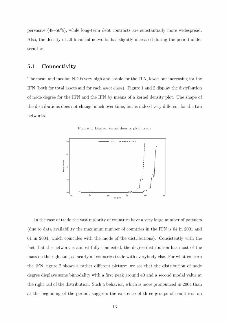
5.1 Connectivity
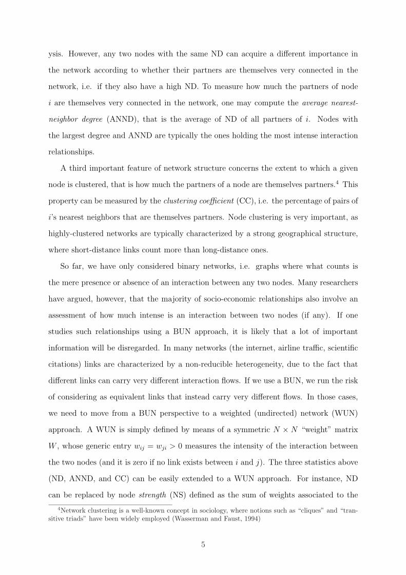
The mean and median ND is very high and stable for the ITN, lower but increasing for the
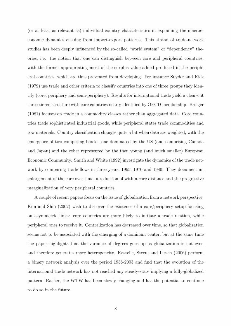
IFN (both for total assets and for each asset class). Figure 1 and 2 display the distribution
of node degree for the ITN and the IFN by means of a kernel density plot. The shape of
the distributions does not change much over time, but is indeed very different for the two
networks.
Figure 1: Degree, kernel density plot: trade
0
.2
.4
.6
.8
Kern
el d
ensi
ty
40 45 50 55 60 65degree
2001 2004
In the case of trade the vast majority of countries have a very large number of partners
(due to data availability the maximum number of countries in the ITN is 64 in 2001 and
61 in 2004, which coincides with the mode of the distributions). Consistently with the
fact that the network is almost fully connected, the degree distribution has most of the
mass on the right tail, as nearly all countries trade with everybody else. For what concern
the IFN, figure 2 shows a rather different picture: we see that the distribution of node
degree displays some bimodality with a first peak around 40 and a second modal value at
the right tail of the distribution. Such a behavior, which is more pronounced in 2004 than
at the beginning of the period, suggests the existence of three groups of countries: an
13

elite of countries connected with everybody else, a larger group of countries with average
connectedness and a periphery of less connected economies.
Figure 2: Degree, kernel density plot: total assets
0
.005
.01
.015
.02
.025Ke
rnel
den
sity
0 20 40 60 80degree
2001 2004
Comparing the distribution of ND in 2001 and 2004, one has the feeling that at least
some peripheral countries have moved to the middle group, which has in fact enlarged
its ranks: in 2004 the distribution is more concentrated around the central peak and the
left-hand tail is thinner. Moreover, the coefficient of variation of node degree is smaller
testifying for a lower dispersion. Yet, given the very short time span of our data, it is very
difficult to assess whether this is the result of a temporary shock or a permanent shift.8
Figure 3: Strength, kernel density plot: trade
0
.5
1
1.5
2
Kern
el d
ensi
ty
0 1 2 3 4strength
2001 2004
8Based on a Kolmogorov-Smirnov test it is not possible to reject the null hypothesis of the twodistributions being equal.
14

The picture changes significantly when we move from BUN to WUN analysis and
weight each link by its intensity. Figure 3 shows that the distribution of node strength for
the ITN is no longer skewed on the left but rather on the right: a majority of countries
holding many weak relationships coexists with a small number of them characterized by
more intense links. This feature gets slightly reduced in subsequent years: in 2004 the
peak is lower and more mass is distributed at higher values of strength.9
Something similar occurs in the case of the IFN (figure 4). As one could possibly
guess, the distribution is even more heavily skewed here than in the case of trade, and
any bimodality disappears.
Figure 4: Strength, kernel density plot: total assets
0
1
2
3
4
Kern
el d
ensi
ty
0 1 2 3 4 5strength
2001 2004
Connectivity as measured by ND and NS has increased for all asset types. Apart for
total assets, it is highest for debt contracts (total debt and long-term one) and lowest for
short-term debt, with cross-border equity holdings somehow in between.
The fact that the ITN is almost fully connected results in the correlation between
ND and NS being not significantly different from zero, as ND varies very little. On the
contrary, the correlation is positive and significant in the case of the IFN. This means
that on average countries with many trading partners tend to hold also more intense
relationships.
In the case of WUN, a further important piece of information is represented by dispar-
9The fact that the number of available countries in the network is smaller in 2004 surely plays a rolein determining the reduction in the peak of the distribution.
15

ity, which tells us whether trade and financial links carry similar weight or rather countries
tend to display few tight links and a large number of feeble ones. Table 2 reports the
mean values of node disparity for the different types of WUN under scrutiny. One can
see that in the case of ITN disparity is low and stable; at the end of the sample period
the IFN based on total assets has reached the same value though it started from a higher
figure. The behavior of disparity for different asset classes is consistent with what we have
found so far, with a higher value for equities, small figures for total and long-term debt
and high disparity for short-term debt, again to testify a rather sparse network populated
by links carrying very different weights.
Table 2: Node disparity
total long shorttrade assets equities debt debt debt
2001 0.13 0.207 0.286 0.203 0.2 0.3562002 0.125 0.215 0.316 0.22 0.215 0.3932003 0.122 0.159 0.265 0.2 0.198 0.3342004 0.117 0.117 0.249 0.172 0.182 0.294
This first set of results allows us to make an important methodological point: if the
study of the ITN and the IFN is carried out from a BUN perspective, one runs the risk of
getting a misleading picture of the underlying phenomena. A weighted network analysis
instead allows one to better appreciate how the intensity of the interaction structure is
distributed across the population.
5.2 Assortativity
Degree and strength statistics are first-order indicators: they only take into account
links to one-step-away partners and do not convey any information on the finer struc-
ture of the network. Indeed, it may well happen that countries having many partners
are only linked with with poorly-connected countries (we call such a network “disassor-
tative”). Conversely, it may be the case that better connected countries also tend to
relate to other well-connected countries (i.e., an “assortative” network). The relation be-
tween average nearest-neighbor degree (ANND) and ND on one side, and between average
16

nearest-neighbor strength (ANNS) and NS on the other allows one to assess the degree
of assortativity that exists within the network. In other words, whether countries choose
as partners nations with the same degree (strength) and whether the relationships with
high/low degree/strength countries follow the magnitude of the interaction.
Table 3: Correlation between node degree (strength) and ANND (ANNS)
total long shorttrade assets equities debt debt debt
BUN: degree – ANND
2001 -0.705 -0.964 -0.916 -0.946 -0.948 -0.5522002 -0.661 -0.957 -0.931 -0.979 -0.976 -0.7242003 -0.572 -0.957 -0.878 -0.948 -0.972 -0.7592004 -0.659 -0.977 -0.922 -0.967 -0.964 -0.830
WUN: strength – ANNS
2001 -0.607 -0.423 -0.401 -0.495 -0.515 -0.3232002 -0.513 -0.392 -0.418 -0.463 -0.488 -0.2772003 -0.494 -0.531 -0.459 -0.596 -0.577 -0.3732004 -0.679 -0.556 -0.485 -0.581 -0.576 -0.376
Table 3 displays the correlation between ND (respectively, NS) and ANND (respec-
tively, ANNS). BUN analysis points toward a strongly disassortative network; this feature
remains evident also in the context of WUN, though weaker in magnitude. Serrano and
Boguna (2003) also find that the ITN is a disassortative network, a result that we can
now extend to the IFN irrespectively of whether one focuses on total assets, bonds or
equities. This implies not only that poorly connected countries preferentially connect
to high degree countries (BUN case), sometimes referred to as hubs, but also that this
core-periphery structure is maintained also in terms of intensity of interactions.
The behavior of financial links, in particular the strong negative correlation for BUN
can probably be explained by the existence of a number of benchmark securities that
enter almost every portfolio. When it comes to measuring the importance of such se-
curities though, assets issued by more peripheral countries become appealing in view of
diversification, so that weighted financial links become more dispersed and the relevance
of hubs diminishes.
17

5.3 Clustering
Clustering measures the local interconnectivity of the network by computing the number
of complete triangles originating from a given country. In other words how many of the
partners of country i are themselves connected to each other. The clustering coefficient
(CC) for BUNs is almost 1 in the case of the ITN, consistently with the previous finding
of a fully connected network, but values are quite high (in the .70–.85 range) for the IFN
as well. The CC is very high in all years and, moreover, it is always larger than network
density: since in a completely random graph the two are equal, our result implies that
the ITN and the IFN are statistically more clustered than if they were random graphs.10
Therefore, countries tend —on average— to establish trade and financial relationships
with partners that are also linked with each other. This sort of “cliquishness” suggests
that regional or local ties still play a very relevant role, where localism has not necessarily
a geographic meaning, but can well be read as the tendency to interact with traditional
partners.11 These can be member of a regional group, countries with similar degree of
development, or simply partners that are historically close.
Does this result hold also if we take into account the intensity or relationships? The
answer is no: the weighted version of the CC (WCC) is not only very low, but also smaller
than its average value in a random graph. Thus, from a weighted perspective, the ITN
and the IFN are on average poorly clustered. Out of the network jargon this implies that
there is some heterogeneity within each group or clique of countries, consistently with
the idea of the existence of a prominent center acting as an hub. It is not difficult to
recognize this portrait in the real world, where in each regional group usually a single
financial center emerges.
A similar mismatch between BUN and WUN results emerges when we look at the
correlation between clustering and node degree or strength. Table 4 shows that while the
CC is negatively related to ND, the WCC and NS display a positive correlation.12 Hence,
10See Appendix A.11Although we have no means to check whether geography plays any role in the game, it is nonetheless
interesting to note that our picture is consistent both with the idea that distance proxies some informa-tion costs (Portes and Rey, 2005), and with the notion that informational asymmetries may depend oninvestors location (Hau, 2001).
12In both cases the correlations are significant at 1%.
18
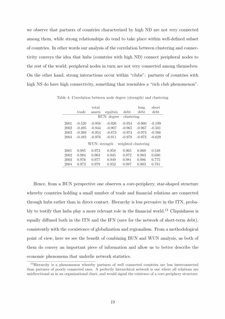
we observe that partners of countries characterized by high ND are not very connected
among them, while strong relationships do tend to take place within well-defined subset
of countries. In other words our analysis of the correlation between clustering and connec-
tivity conveys the idea that hubs (countries with high ND) connect peripheral nodes to
the rest of the world; peripheral nodes in turn are not very connected among themselves.
On the other hand, strong interactions occur within “clubs”: partners of countries with
high NS do have high connectivity, something that resembles a “rich club phenomenon”.
Table 4: Correlation between node degree (strength) and clustering
total long shorttrade assets equities debt debt debt
BUN: degree – clustering
2001 -0.520 -0.958 -0.926 -0.954 -0.960 -0.1992002 -0.495 -0.944 -0.907 -0.965 -0.967 -0.5012003 -0.369 -0.954 -0.873 -0.974 -0.973 -0.5662004 -0.482 -0.976 -0.911 -0.978 -0.972 -0.629
WUN: strength – weighted clustering
2001 0.985 0.973 0.958 0.965 0.969 0.5492002 0.984 0.963 0.945 0.972 0.983 0.6902003 0.976 0.977 0.949 0.981 0.986 0.7752004 0.973 0.979 0.952 0.987 0.983 0.781
Hence, from a BUN perspective one observes a core-periphery, star-shaped structure
whereby countries holding a small number of trade and financial relations are connected
through hubs rather than in direct contact. Hierarchy is less pervasive in the ITN, proba-
bly to testify that hubs play a more relevant role in the financial world.13 Cliquishness is
equally diffused both in the ITN and the IFN (save for the network of short-term debt),
consistently with the coexistence of globalization and regionalism. From a methodological
point of view, here we see the benefit of combining BUN and WUN analysis, as both of
them do convey an important piece of information and allow us to better describe the
economic phenomena that underlie network statistics.
13Hierarchy is a phenomenon whereby partners of well connected countries are less interconnectedthan partners of poorly connected ones. A perfectly hierarchical network is one where all relations areunidirectional as in an organizational chart, and would signal the existence of a core-periphery structure.
19

5.4 Network properties and per capita GDP
An interesting issue to explore concerns the extent to which network-specific indicators
correlate with country wealth. For example, do countries with a higher per-capita GDP
(pcGDP) maintain more and stronger relationships? Are the rich more clustered? To
answer these questions, we study the correlation patterns existing between our network-
specific measures (degree, strength, clustering) and country pcGDP.
Table 5: Correlation between node degree/strength and per capita GDP
total long shorttrade assets equities debt debt debt
BUN: degree – pcGDP
2001 0.156 0.015 -0.043 0.037 0.031 -0.0452002 0.189 -0.027 -0.076 0.008 0.013 -0.0172003 0.197 0.013 -0.072 0.045 0.035 -0.0252004 0.182 0.000 -0.093 0.073 0.076 -0.026
WUN: strength – pcGDP
2001 0.466 0.577 0.551 0.582 0.584 0.5052002 0.452 0.579 0.553 0.573 0.570 0.5092003 0.431 0.569 0.530 0.568 0.569 0.4842004 0.411 0.576 0.534 0.578 0.573 0.506
As far as ND is concerned, its correlation with pcGDP is low and never statistically
significant (not even for the ITN). Yet, concluding that there is not any relation between
the position within the network (connectivity) and pcGDP would be wrong as the latter
displays a positive and significant (at 1%) correlation with NS, as reported in the lower
panel of table 5. This is to say that once we control for the intensity of trade and financial
connections we observe that richer countries are better connected than poorer economies.
The correlation is somewhat smaller in the case of the ITN, while different asset types do
not display marked differences.
Results for clustering-pcGDP correlations mimic those obtained in the case of clus-
tering and ND/NS. Hence, our BUN analysis suggests the existence of a hierarchical
structure in terms of number of partners: rather than on the position within the network
this hierarchy is now based on the degree of economic development as measured by per
capita income. On the contrary, for what concerns the strength of relations (WUN) we
20

observe some sort of cliquishness: partners of countries with a high pcGDP are more
interconnected than those of poorer countries.
5.5 Centrality
So far we have treated nodes as anonymous, not considering which countries display higher
or lower network properties. Now we address the role each country plays in the ITN and
in the IFN by means of a measure of centrality. By doing so we will be able to explicitly
characterize the core and the periphery of the networks, whose existence is hinted at by
our results, and to compare them.
Figure 5: Random Walk Betweenness Centrality, kernel density plot
0
5
10
15
Kern
el d
ensi
ty
0 .2 .4 .6 .8 1Random Walk Betweenness Centrality (2004)
Trade Total Assets
We compute random walk betweenness centrality (RWBC, see Section 2 and Appendix
A) for each of the countries in the ITN and IFN and use the results to classify them as
part of the core or of the periphery. It turns out that —due to the high density that
characterizes both the ITN and the IFN— the binary version of RWBC displays very
little variation and, in addition, it is almost perfectly correlated with ND: as a result, in
what follows we will focus only on the weighted version of RWBC.14
Figure 5 presents the distribution of weighted RWBC for both the ITN and the IFN
of total assets in 2004. The pattern observed for both networks has not changed over the
period considered in the study, so that figure 5 gives a good representation of the overall
14A second reason is that so far weighted indicators seem to give a better representation of the networkstructure, and in particular to hint more directly to a core-periphery structure.
21

behavior. Similarly, there are no discernable differences across asset types and therefore we
focus on the discussion of the results based on total assets. Both distributions are heavily
skewed to the right, confirming the hypothesis of a clear-cut core-periphery structure.
Table 6: Composition of the core
2001 2002 2003 2004Based on Trade
USA USA USA USAUK UK UK UKGermany Germany Germany GermanyFrance France France FranceJapan Netherlands Netherlands JapanItaly Japan Japan ItalyRussia Italy Italy
Based on Total Assets
USA USA USA USAUK UK UK UKGermany Germany Germany GermanyLuxembourg Luxembourg Luxembourg LuxembourgFrance France France FranceJapan Japan Netherlands NetherlandsItaly Italy Japan
To identify the countries actually belonging to the core we (arbitrarily) impose a
threshold at the 90th percentile of RWBC: hence, only countries with a value of the
RWBC index within the top 10% are considered core.15 The number of countries in the
core ranges between 7 (2001–2003) and 6 (2004) and its composition is quite stable (see
table 6). In fact in the core we find all the “usual suspects” with the only a few exceptions:
the presence of Russia in the core of the trade network in 2001 seems occasional as the
country drops out from it in following years and actually never comes close to rejoin the
group. In both the ITN and the IFN the Netherlands switch in and out of the core,
constantly displaying a limit value of centrality. The core of both networks is basically
made up of the same countries, with the notable exception of Luxembourg, which plays
a central node with respect to financial assets, but not with respect to trade flows.
Finally, the analysis of the correlation between per capita GDP and node betweenness
15The same results are obtained once we substitute this relative criterion with an absolute one andattribute core status to those countries displaying values of centrality above the mean plus one standarddeviation.
22

Table 7: Correlation between weighted centrality and per capita GDP
total long shorttrade assets equities debt debt debt
2001 0.446 0.505 0.509 0.517 0.520 0.5152002 0.427 0.500 0.493 0.503 0.505 0.2342003 0.394 0.484 0.463 0.484 0.488 0.4932004 0.366 0.476 0.453 0.490 0.481 0.513
centrality reveals a similar pattern to that observed for the relationship between node
strength and pcGDP.16 It should be noted that even though the correlation is positive
for both networks, it is higher for the IFN, further testifying that international trade
integration is more widespread. The results presented in table 7 show that the correlation
between pcGDP and RWBC is not only higher for the case of the ITN, but also that it has
been steadily declining in the period under scrutiny. This pattern suggests that a higher
degree of international economic integration through capital flows is more likely related
to a higher pcGDP than a high degree of international economic integration through
international trade.
6 Conclusions and Possible Extension
The paper has investigated the properties of the ITN and the IFN using both a binary
and a weighted network approach. From a methodological point of view, our paper is
the first one —to the best of our knowledge— addressing this issue from a weighted
network perspective. Indeed, many findings obtained by only looking at the number of
relationships that any country maintains are completely reversed if one takes into account
the relative intensity of links. Our results show that combining binary and weighted
analysis can deliver more precise and thorough insights as far as the topological structure
and properties of the ITN and the IFN are concerned. Expectedly, the paper finds that
the ITN is more densely connected than the IFN and that the degree of international
financial integration varies with asset type: it is highest for long-term debt contracts,
16This is expected since one of the interpretations of node strength is related to the degree of influencethat a given node has on the network or to what extent other nodes depend on a given node; also, thecorrelation between RWBC and NS is very high.
23

somewhat lower for equities and rather low for short-term debt, which is characterized by
a sparse network.
As compared to standard international-trade statistical investigations, network analy-
sis allows the researcher to explore not only first-order phenomena associated to the pat-
terns of trade and financial integration of any given country (e.g. the degree of openness
to trade or the share of foreign assets in the portfolio), but also second- and higher-order
empirical facts. In particular, we show that richer countries tend to be better linked and
to form groups of tightly connected economies. These cliques are built along the lines of
both connectivity and richness and can be seen as a sign of the persistent relevance of
local relations. However, the growing importance of global links is testified by the disas-
sortative feature of both the ITN and the IFN: poorly connected nodes tend to connect
to central ones and use them as hubs to access the rest of the network.
For what concerns future research, a natural extension of our work entails exploring
the role of geographic proximity in shaping the ITN and the IFN: this might allow us
to better determine the relative importance of global and local links, and whether the
two act as substitutes or rather complement each other. Along this line, an interesting
question concerns the impact of regional integration (trade agreements, but also monetary
integration) on the characteristics of the network. Second, along the line of Kali and Reyes
(2007), we would like to match topological properties with country-specific variables to
see how the structure of the ITN and IFN is shaped by (and shapes) macroeconomic
dynamics.
Acknowledgments
Thanks to Marc Barthelemy, Helmut Elsinger, Diego Garlaschelli, Bertrand Groslam-
bert, Cal Muckley, and participants at the 5th INFINITI Conference for their useful and
insightful comments on earlier drafts of the paper. All usual disclaimers apply.
24

References
Baele, L., A. Ferrando, P. Hordahl, E. Krylova and C. Monnet (2004), “Measuring Euro-
pean Financial Integration”, Occasional Paper 14, ECB.
Barrat, A., M. Barthelemy, R. Pastor-Satorras and A. Vespignani (2004), “The architec-
ture of complex weighted networks”, Proceedings of the National Academy of Sciences,
101: 3747–52.
Bekaert, G. and C. Harvey (2003), “Emerging markets finance”, Journal of Empirical
Finance, 10(1-2): 3–56.
Breiger, R. (1981), “Structure of economic interdependence among nations”, in Blau,
P. M. and R. K. Merton (eds.), Continuities in structural inquiry, pp. 353–80. Sage,
Newbury Park, CA.
Fagiolo, G. (2006), “Directed or Undirected? A New Index to Check for Directionality of
Relations in Socio-Economic Networks”, Economics Bulletin, 3: 1–12, available on-line
at http://economicsbulletin.vanderbilt.edu/2006/volume3/EB-06Z10134A.pdf.
Fisher, E. and F. Vega-Redondo (2006), “The Linchpins of a Modern Economy”, Working
paper, Cal Poly.
Garlaschelli, D. and M. Loffredo (2004), “Fitness-Dependent Topological Properties of
the World Trade Web”, Physical Review Letters, 93: 188701.
Garlaschelli, D. and M. Loffredo (2005), “Structure and evolution of the world trade
network”, Physica A, 355: 138–44.
Goldberg, L., J. Lothian and J. Okunev (2003), “Has International Financial Integration
Increased?”, Open Economies Review, 14: 299–317.
Granovetter, M. (1974), Getting a Job: A Study of Contracts and Careers. Cambridge,
MA, Harvard University Press.
25
Hau, H. (2001), “Location Matters: An Examination of Trading Profits”, Journal of
Finance, 56(5): 1959–83.
Kali, R. and J. Reyes (2005), “Financial contagion on the International Trade Network”,
Unpublished Manuscript.
Kali, R. and J. Reyes (2007), “The Architecture of Globalization: A Network Approach to
International Economic Integration”, Journal of International Business Studies, Forth-
coming.
Kastelle, T., J. Steen and P. Liesch (2006), “Measurig globalisation: an evolutionary
economic approach to tracking the evolution of international trade”, Paper presented
at the DRUID Summer Conference on Knowledge, Innovation and Competitiveness:
Dynamycs of Firms, Networks, Regions and Institutions - Copenhagen, Denemark,
June 18–20.
Kim, S. and E.-H. Shin (2002), “A Longitudinal Analysis of Globalization and Regional-
ization in International Trade: A Social Network Approach”, Social Forces, 81: 445–71.
Li, X., Y. Y. Jin and G. Chen (2003), “Complexity and synchronization of the World
trade Web”, Physica A: Statistical Mechanics and its Applications, 328: 287–96.
Milesi-Ferretti, G. M. and G. M. Lane (2006), “The External Wealth of Nations Mark
II: Revised and Extended Estimates of Foreign Assets and Liabilities, 1970-2004”, IMF
Working Papers 06/69, International Monetary Fund.
Milgram, S. (1967), “The small world problem”, Psychology Today, 2: 60–67.
Newman, M. (2005), “A measure of betweenness centrality based on random walks”,
Social Networks, 27: 39–54.
Onnela, J., J. Saramaki, J. Kertesz and K. Kaski (2005), “Intensity and coherence of
motifs in weighted complex networks”, Physical Review E, 71: 065103.
Padgett, J. and C. Ansell (1993), “Robust action and the rise of the Medici, 1400-1434”,
American Journal of Sociology, 98: 1259–1319.
26

Portes, R. and H. Rey (2005), “The determinants of cross-border equity flows”, Journal
of International Economics, 65: 269–96.
Rapoport, A. and W. Horvath (1961), “A study of a large sociogram”, Behavioral Science,
6: 279–291.
Scott, J. (2000), Social Network Analysis: A Handbook. London, Sage.
Serrano, A. and M. Boguna (2003), “Topology of the World Trade Web”, Physical Review
E, 68: 015101(R).
Smith, D. and D. White (1992), “Structure and Dynamics of the Global Economy: Net-
work Analysis of International Trade, 1965-1980”, Social Forces, 70: 857–93.
Snyder, D. and E. Kick (1979), “Structural position in the world system and economic
growth 1955-70: A multiple network analysis of transnational interactions”, American
Journal of Sociology, 84: 1096–126.
Wasserman, S. and K. Faust (1994), Social Network Analysis. Methods and Applications.
Cambridge, Cambridge University Press.
Appendix A: Statistical Analysis of Binary and Weighted
Networks
In this appendix, we present some more formal definitions of the statistics introduced in
Section 2 for both binary and weighted networks.
Consider a network composed of N nodes. Let W = {wij} be a N ×N weight matrix
(not necessarily symmetric), where wij ∈ [0, 1] and wii = 0 for all i. The binary case will
imply that wij ∈ {0, 1}. We assume that a link from i to j exists if and only if wij > 0.
The adjacency N × N matrix A = {aij}, where aij ∈ {0, 1}, is thus defined from W by
letting aij = 1 iff wij > 0 (and zero otherwise).
In what follows, we will also define X(i) as the i-th row of matrix X, and X [k] as the
matrix obtained from X by raising to k each entry.
27

Binary undirected networks
Let us suppose that the underlying graph is binary and undirected and let A be its
adjacency matrix. The degree of node i (or node degee, ND) is defined as
di =∑
j
aij = A(i)1, (1)
where 1 is the N -vector made of all ones.
Similarly, the average nearest-neighbor degree (ANND) of node i reads:
anndi = d−1i
∑
j
aijdj = d−1i
∑
j
∑
h
aijajh =A(i)A1
A(i)1. (2)
Finally, node i’s clustering coefficient (CC), defined as the ratio of the number of
triangles with i as one vertex, to the maximum number of triangles that node i could
have formed given its degree, is equal to:
Ci(A) =12
∑
j 6=i
∑
h 6=(i,j) aijaihajh
12di(di − 1)
=(A3)ii
di(di − 1). (3)
Notice that in a random graph where links are in place, independently of each other, with
a probability p > 0, the expected value for the CC is equal to p.
Weighted undirected networks
Let us now assume that the underlying graph is weighted and undirected and let W be
its weight matrix. First, node strength of i is defined as:
si =∑
j
wij = W(i)1. (4)
Furthermore, the average nearest-neighbor strength (ANNS) of i is computed as the arith-
metic mean of strengths of i’s neighbors as follows:
annsi = d−1i
∑
j
aijsj = d−1i
∑
j
∑
h
aijwjh =A(i)W1
A(i)1. (5)
28

Sometimes, it is also useful to define “node disparity” among (concentration of) i’s weights
as follows:
hi =(N − 1)
∑
j
(
wij
si
)2
− 1
N − 2=
(N − 1) 1s2i
∑
j w2ij − 1
N − 2=
(N − 1)W
[2](i)
1
(W(i)1)2− 1
N − 2. (6)
As far as the weighted version of the CC for WUN is concerned, we focus here on the
extension of the CC to WUN originally introduced in Onnela, Saramaki, Kertesz, and
Kaski (2005):
Ci(W ) =12
∑
j 6=i
∑
h 6=(i,j) w13ijw
13ihw
13jh
12di(di − 1)
=(W [ 1
3 ])3ii
di(di − 1), (7)
where we define W [ 1k ] = {w
1k
ij}, i.e. the matrix obtained from W by taking the k-th root of
each entry. The index Ci ranges in [0, 1] and reduces to Ci when weights become binary.
Furthermore, it takes into account weights of all edges in a triangle (but does not consider
weights not participating in any triangle) and is invariant to weight permutation for one
triangle. The expected value of the weighted CC in a random graph where links are in
place, independently of each other, with a probability p > 0, is equal to (34)3p.
Random-Walk Betweenness Centrality (RWBC)
Suppose the underlying graph, interpreted as a current circuit, is a WUN and let W be
its weight matrix and s the N × 1 strength vector. Following Newman (2005) and Fisher
and Vega-Redondo (2006), consider a generic node i for which we want to compute the
RWBC and an impulse generated from node h (the source) and working its way to node
k (the target). Let f(h, k) be the “source” N × 1-vector such that fi(h, k) = 1 if i = h,
fi(h, k) = −1 if i = k, and 0 otherwise. Define by v(h, k) the N × 1-vector of node
voltages. Newman (2005) shows that Kirchoff’s law of current conservation implies that:
v(h, k) = [D − W ]−1f(h, k), (8)
where D = diag(s) and [D −W ]−1 is computed using the Moore-Penrose pseudo-inverse.
This in turn implies that the current (i.e. intensity of interaction) flowing through
29

node i, originated from h and getting to k, is given by:
Ii(h, k) =1
2
∑
j
|vi(h, k) − vj(h, k)|, (9)
where Ih(h, k) = Ik(h, k) = 1.
It is then straightforward to define node-i RWBC as:
RWBCi =
∑
h
∑
k 6=h Ii(h, k)
N(N − 1). (10)
30

Appendix B: Countries in the sample
4c—Trade CPIScode Country 2001 2002 2003 2004 2001 2002 2003 2004213 Argentina x x x x x x x x314 Aruba x x – – x x – –193 Australia x x x x x x x x122 Austria x x x x x x x x313 Bahamas, The x x x – x x x –419 Bahrain x x x x x x x x316 Barbados x x x x x x x x124 Belgium x x x x x x x x223 Brazil x x x x x x x x918 Bulgaria x x x x x x x x156 Canada x x x x x x x x228 Chile x x x x x x x x233 Colombia x x x x x x x x238 Costa Rica x x x x x x x x423 Cyprus x x x x x x x x935 Czech Republic x x x x x x x x128 Denmark x x x x x x x x469 Egypt x x x x x x x x939 Estonia x x x x x x x x172 Finland x x x x x x x x132 France x x x x x x x x134 Germany x x x x x x x x174 Greece x x x x x x x x532 Hong Kong SAR x x x x x x x x944 Hungary x x x x x x x x176 Iceland x x x x x x x x536 Indonesia x x x x x x x x178 Ireland x x x x x x x x115 Isle of Man – – – – x x x –436 Israel x x x x x x x x136 Italy x x x x x x x x158 Japan x x x x x x x x916 Kazakhstan x x x x x x x x542 Korea, Republic x x x x x x x x446 Lebanon x x x x x x x x137 Luxembourg x x x x x x x x546 Macao SAR x x – – x x – –548 Malaysia x x x x x x x x181 Malta x x x x x x x x684 Mauritius x x x x x x x x273 Mexico x x x x x x x x138 Netherlands x x x x x x x x196 New Zealand x x x x x x x x142 Norway x x x x x x x x564 Pakistan x x x x x x x x283 Panama x x x x x x x x566 Philippines x x x x x x x x964 Poland x x x x x x x x182 Portugal x x x x x x x x968 Romania x x x x x x x x922 Russian Fed x x x x x x x x
(continued on next page)
31

Trade CPIScode Country 2001 2002 2003 2004 2001 2002 2003 2004576 Singapore x x x x x x x x936 Slovak Republic x x x x x x x x199 South Africa x x x x x x x x184 Spain x x x x x x x x144 Sweden x x x x x x x x146 Switzerland x x x x x x x x578 Thailand x x x x x x x x186 Turkey x x x x x x x x926 Ukraine x x x x x x x x112 United Kingdom x x x x x x x x111 United States x x x x x x x x298 Uruguay x x x x x x x x846 Vanuatu x x x x x x x x299 Venezuela x x x x x x x x
number of countries 64 64 62 61 65 65 63 61x available; – not available (or not used)
32