International Spillovers and Guidelines for Policy Cooperation

Anton Korinek Johns Hopkins University

Paper presented at the 15th Jacques Polak Annual Research Conference Hosted by the International Monetary Fund Washington, DCNovember 13–14, 2014 The views expressed in this paper are those of the author(s) only, and the presence

of them, or of links to them, on the IMF website does not imply that the IMF, its Executive Board, or its management endorses or shares the views expressed in the paper.

1155TTHH JJAACCQQUUEESS PPOOLLAAKK AANNNNUUAALL RREESSEEAARRCCHH CCOONNFFEERREENNCCEE NNOOVVEEMMBBEERR 1133––1144,, 22001144

International Spillovers andGuidelines for Policy Cooperation

A Welfare Theorem for National Economic Policymaking∗

Anton KorinekJohns Hopkins University and NBER

Draft: October 2014

Abstract

In an interconnected world, national economic policies lead to internationalspillover effects. This has recently raised concerns about global currency wars.We show that international spillover effects are Pareto effi cient and that thereis no role for global coordination if three conditions are met: (i) national policy-makers act as price-takers in the international market, (ii) national policymak-ers possess a complete set of instruments to control the external transactionsof their country and (iii) there are no imperfections in international markets.Under these conditions, international spillover effects constitute pecuniary ex-ternalities that are mediated through market prices and do not give rise toineffi ciency. We cover four applications: policies to correct growth externali-ties, aggregate demand externalities in a liquidity trap, spillovers from fiscalpolicy, and exchange rate stabilization policy. Conversely, if any of the threeconditions we identify is violated, we show how global cooperation can improvewelfare. Examples that we cover include beggar-thy-neighbor policies, countrieswith imperfect instruments, and incomplete global financial markets.

JEL Codes: F34, F41, H23Keywords: economic policy cooperation, spillovers, externalities,

currency wars

∗I would like to thank Kyle Bagwell, Olivier Blanchard, Emmanuel Farhi, Rex Ghosh, SebnemKalemli-Ozcan, Jonathan Ostry and Joseph Stiglitz for detailed conversations on the topic. ChangMa and Jonathan Kreamer provided excellent research assistance. Furthermore, I gratefully ac-knowledge financial support from the IMF Research Fellowship and from CIGI/INET.

1

1 Introduction

In a globally integrated economy, national economic policies generate internationalspillover effects. This has recently led to considerable controversy in internationalpolicy circles and has raised concerns about global currency wars.1 The contributionof this paper is to provide a broad set of suffi cient conditions under which nationalpolicymaking in pursuit of domestic objectives leads to Pareto effi cient global out-comes. In other words, our paper extends the first welfare theorem to the interactionsof national economic policymakers in a multi-country setting. Under the conditionsthat we identify, all international spillover effects are Pareto effi cient and there isno case for international policy cooperation. Conversely, our paper describes howinternational policy cooperation can generate Pareto improvements if one of theseconditions is violated.We develop a multi-country general equilibrium framework that nests a broad class

of open economy macro models and that is able to capture a wide range of domesticmarket imperfections and externalities. We assume that each country encompasses aset of optimizing private agents as well as a policymaker who has policy instrumentsto affect the domestic and international transactions of the economy. When thepolicymaker in a given country changes her policy instruments, she influences theactions of domestic consumers, which in turn lead to general equilibrium adjustmentsthat may entail spillover effects to other economies.2

We show that the spillovers created by national economic policymaking are Paretoeffi cient and that there is no need for global cooperation if three conditions are met:(i) national policymakers act competitively, i.e. they act as price-takers in the in-ternational market, (ii) if there are domestic externalities, national policymakers ei-ther possess a suffi cient set of policy instruments to control them domestically ora complete set of external policy instruments, and (iii) there are no imperfectionsin international markets. Under these three conditions, we can view national poli-cymakers as competitive agents in a well-functioning global market, and so the firstwelfare theorem applies. Therefore international spillover effects constitute pecuniaryexternalities that are mediated through market prices and do not give rise to ineffi -ciency. By implication, spillover effects by themselves should not be viewed as a signof ineffi ciency.We obtain our results by observing that, under quite general conditions, we can

condense the welfare function of each country into a reduced-form welfare functionV (·) in which the only argument is a vector of the country’s international transac-tions. Condition (i) ensures that policymakers are price-takers and that there are

1The term “curreny war”was coined by the Brazilian finance minister Guido Mantega in Septem-ber 2010 to describe policies of the US a number of Asian countries that had the effect of depreciatingtheir exchange rates. For detailed discussions on this subject see e.g. Gallagher et al. (2012), Jeanneet al. (2012), Ostry et al. (2012) and Stiglitz (2012).

2For a detailed review of both the theoretical and empirical literature on spillovers, see for exampleKalemli-Ozcan et al. (2013).

2

no monopolistic distortions; condition (ii) of complete policy instruments guaranteesthat each domestic policymaker has the instruments to implement her desired exter-nal allocation subject to a country’s external budget constraint; condition (iii), thatthere are no imperfections in international markets, ensures that the marginal rates ofsubstitution of all countries are equated in equilibrium. As a result, we can apply thefirst welfare theorem at the level of national policymakers, interpreting V (·) as theutility functions of competitive agents in a complete market. Our model is generalenough to allow for a wide range of domestic market imperfections, including pricestickiness, financial constraints, incentive/selection constraints, missing or imperfectdomestic markets, etc.If any of the three conditions we identified is violated, spillover effects generally

lead to ineffi ciency, and global cooperation among national policymakers can generallyimprove welfare. Following the three conditions above, such cooperation works alongthree dimensions: (i) It ensures that countries refrain from monopolistic behaviorand act with “benign neglect”towards international variables. (ii) If countries facedomestic externalities but have incomplete/imperfect instruments to address them,then welfare is improved if those countries with better instruments or better-targetedinstruments assist those without. (iii) If imperfections in international markets leadto ineffi ciency, then global coordination is necessary to restore effi ciency since theimperfections are outside of the domain of individual national policymakers. Weprovide examples that characterize the scope for coordination in each of the threecases.The types of cooperation described in points (ii) and (iii) typically implement

second-best equilibria that take the set of available policy instruments and marketsas given but make more effi cient use of them. There is also a scope for first-bestpolicies in these areas: global cooperation may increase effi ciency by creating moreor better policy instruments, or by reducing imperfections in international markets.3

Our analysis suggests that the case for global cooperation disappears the closer wemove to the ideal of perfect external instruments and international markets, providedthat national economic policymakers continue to act competitively.

We apply our theoretical analysis to a number of practical applications, manyof which have led to controversy in international policy circles in recent years. Ourfirst application, chosen because it provides the simplest illustration of our results,is to analyze an economy in which international capital flows generate technologicalexternalities. An important example that is frequently referred to by policymakersin developing economies are learning-by-exporting effects. We show that a national

3A number of recent reforms in the global financial architecture follow this principle: for example,Basel III provides policymakers with new counter-cyclical capital buffers (better instruments), recentIMF proposals allow countries to use capital controls (new instruments; see Ostry et al, 2011), andswap lines between advanced economy central banks provide new forms of liquidity insurance (morecomplete markets). A standard caveat in the theory of the second-best applies: moving closer to thecase of perfect markets and perfect instruments does not always imply more effi cient outcomes.

3

policymaker finds it optimal to correct technological externalities via current accountor capital account intervention. Furthermore, as long as the three conditions identifiedabove are satisfied, this policy intervention is effi cient from a global perspective,i.e. global cooperation cannot achieve a Pareto superior outcome. We extend ouranalysis to domestic technological externalities and show that our results continueto hold even if capital account intervention is just a second-best policy measure tocorrect learning-by-doing externalities in the domestic economy.Our second application describes an economy that suffers from a shortage of ag-

gregate demand that cannot be corrected using domestic monetary policy because ofa binding zero-lower-bound on nominal interest rates. In such a situation, a nationaleconomic policymaker finds it optimal to impose controls on capital inflows or to sub-sidize capital outflows in order to mitigate the shortage in demand. Under the threeconditions discussed earlier, this behavior leads, again, to a Pareto effi cient globalequilibrium.Our third application analyzes the incentives for the optimal level of fiscal spend-

ing. If a domestic policymaker chooses how much fiscal spending to engage in basedon purely domestic considerations, we show that the resulting global equilibrium isPareto effi cient under the three discussed conditions. In the context of fiscal policy, itis of particular importance that the domestic policymaker needs to act competitively,i.e. with benign neglect towards the international price effects of her policy actions.In particular, if the policymaker strategically reduces her stimulus in order to ma-nipulate its terms-of-trade, then the resulting equilibrium is ineffi cient and generallyexhibits insuffi cient stimulus. During the Great Recession, this observation has ledmany policymakers to argue that it is necessary to coordinate on providing fiscalstimulus since part of the stimulus spills over to other countries.Our fourth application analyzes an economy in which there are heterogeneous do-

mestic agents who face incomplete risk markets and cannot insure against fluctuationsin the country’s real exchange rate. We show that a national economic policymakercan improve welfare by intervening in the economy’s capital account to stabilize theeconomy’s real exchange rate. This constitutes a second-best policy tool to insuredomestic agents. Again, the outcome is Pareto effi cient under the three conditionsidentified above. This illustrates that our results on global Pareto effi ciency continueto hold even if a national planner pursues purely distributive objectives or implementsdomestic political preferences, as long as we abstain from paternalism, i.e. as long asthe global planning problem that is used to evaluate Pareto effi ciency respects thosedomestic objectives and preferences.In each of the described applications, we show that the spillover effects from pol-

icy intervention are effi cient under the idealized circumstances captured by the threeconditions for effi ciency. Any arguments about the desirability of global policy coor-dination therefore needs to be made on the basis of deviations from these conditions.Our paper therefore concludes by describing the case for coordination in each of thesecircumstances.

4

We continue our analysis by carefully examining the case for economic policycoordination when at least one of the three conditions is violated: When condition(i) is violated and policymakers internalize their market power, coordination shouldaim to restrict monopolistic behavior so as to maximize gains from trade. This hasbeen well understood at least the rebuttal of mercantilism by Smith (1776).4 Thisapplies not only to external policy measures but also to all domestic policies thataffect international prices, such as e.g. fiscal policy. We add to this literature byproviding general conditions for the direction of monopolistic intervention that helpto distinguish monopolistic intervention from intervention to correct domestic marketimperfections. However, we also show that there are ample circumstances under whichit is diffi cult to distinguish monopolistic from corrective intervention. Furthermore,we show that domestic policies will only be distorted with monopolistic objectives ifa country faces restrictions on its set of external policy instruments. For a detaileddiscussion on how to achieve policy agreements to abstain from monopolistic behaviorsee Bagwell and Staiger (2002).Condition (ii) implies that there may be a case for international policy cooperation

when policymakers possess an incomplete set of policy instruments. If a countrysuffers from domestic externalities, we show that the global equilibrium is constrainedPareto effi cient if domestic policymakers either have suffi cient domestic instruments todirectly correct the externalities in the domestic economy (e.g. to stimulate aggregatedemand when it is insuffi cient) or have a complete set of external policy instrumentsso that the indirect effects of external transactions on domestic externalities canbe corrected (e.g. to tax capital inflows when aggregate demand is insuffi cient).Conversely, if a country suffers from externalities and both domestic and externalpolicy instruments are incomplete, then international policy cooperation can generallyachieve a Pareto improvement. Effi cient allocations require that countries with betterinstruments or better-targeted instruments assist those without. For example, if acountry experiences externalities from capital inflows but has no instrument to controlthem, welfare is improved if other countries control their capital outflows.The observation that incomplete policy instruments make it desirable to coordi-

nate policy has a rich intellectual tradition, going back to the targets and instrumentsapproach of Tinbergen (1952) and Theil (1968). They observed in a reduced-formsetting that incomplete instruments may give rise to a role for economic policy coop-eration. Our contribution to this literature is to embed the Tinbergen-Theil approachinto a general equilibrium framework in which optimizing individual agents interact ina market setting. This leads to a number of novel findings. First, we show that manyof the spillover effects that would suggest a role for cooperation in the Tinbergen-Theil

4This observation also underlies much of modern optimal tariff theory. See e.g. Bagwell andStaiger (2002) for a modern treatment in the trade literature, or Costinot et al. (2014) and De Paoliand Lipinska (2013) for recent contributions that focus on intertemporal rather than intratemporaltrade. Farhi and Werning (2012) emphasize this motive for cooperation in a multi-country NewKeynesian framework. Persson and Tabellini (1995) survey implications for macroeconomic policy.

5

framework actually constitute effi cient pecuniary externalities. Once the optimizingbehavior of private agents is taken into account, a wide range of spillovers can beconsidered as effi cient. Secondly, monopoly power and incomplete markets createindependent roles for cooperation even if the set of policy instruments is complete.5

Condition (iii) requires that all international transactions take place in completemarkets and at flexible prices to ensure effi ciency. This is a well-known condition forthe first welfare theorem and has spurred a significant body of literature in the contextof general equilibrium models with individual optimizing agents (see e.g. Geanakoplosand Polemarchakis, 1986; Greenwald and Stiglitz, 1986, for a general treatment). Inour analysis, we interpret national economic policymakers who abstain frommonopolydistortions as competitive agents who interact in an international market and showthat the same effi ciency results hold.6

The remainder of the paper is structured as follows: Section 2 introduces our modelsetup and examines its welfare properties, stating our main result on when spilloversare effi cient. Section 4 provides a number of illustrations of our results. Sections5 to 7 examine the case for international policy coordination when policymakersact monopolistically, are constrained in their policy instruments or face incompleteinternational markets. The final section concludes.

2 Model Setup

Our model describes a multi-country economy in which each country consists of a con-tinuum of private agents as well as a domestic policymaker. Both maximize domesticwelfare subject to a set of constraints on their domestic allocations and a standardbudget constraint on their external transactions. In order to create an interestingrole for policy intervention, we distinguish between individual and aggregate alloca-tions so as to capture the potential for externalities. An individual takes aggregateallocations as given, whereas the domestic planner employs her policy instruments toaffect aggregate allocation so as to correct for domestic externalities. Our frameworknests a wide range of open economy macro models in which there is a case for policyintervention, as we illustrate in a number of examples below.

Countries We describe a world economy with N ≥ 2 countries indexed by i =1, ...N . The mass of each country i in the world economy is ωi ∈ [0, 1], where ΣN

i=1ωi =

1. A country with ωi = 0 corresponds to a small open economy.

5In the more recent literature, Jeanne (2014) provides an interesting example where the coordi-nation of macroprudential policies is warranted because of missing policy instruments.

6Recent applications in an international context include Bengui (2013) who analyzes the needfor coordination on liquidity policies when global markets for liquidity are incomplete, and Jeanne(2014) who analyzes a world economy in which agents are restricted to trading bonds denominatedin the currency of a single country.

6

Private Agents In each country i, there is a continuum of private agents of mass1. We denote the allocations of individual private agents by lower-case variables andthe aggregate allocations of the country by upper-case variables.A representative private agent obtains utility according to a function

U i(xi)

(1)

where xi is a column vector of domestic variables that includes all variables relevantfor the utility of domestic agents, for example the consumption of goods or leisure.We assume that U i (xi) is increasing in each element of xi and quasiconcave.To keep notation compact, xi also includes all domestic variables, including those

that do not directly yield utility but that we want to keep track of, for example thecapital stock ki in models of capital accumulation. For such variables, ∂U i/∂ki = 0.

External Budget Constraint We denote the international transactions of privateagents by a column vector of net imports mi that are traded at an international pricevector Q. Private agents have initial external net worth wi0 and may be subject toa vector of tax/subsidy instruments τ i that is imposed by the domestic policymaker.We denote by Q

1−τ i the element-by-element (Hadamard) division of the price vectorQ by the tax vector (1− τ i), which are both row vectors, and by Q · mi the innerproduct of the price and quantity vectors. The external budget constraint of domesticagents is then

Q

1− τ i ·mi ≤ wi0 + T i (2)

Any tax revenue is rebated as a lump sum transfer T i = τ iQ1−τ i ·m

i. If taxes are zero,then the budget constraint reduces to the country i external constraint Q ·mi ≤ wi0.

Domestic Constraints We assume that the representative agent in country i issubject to a collection of constraints, which encompass domestic budget constraintsand may include any financial, incentive/selection, or price-setting constraints as wellas restrictions imposed by domestic policy measures,

f i(mi, xi,M i, X i, ζ i, Zi

)≤ 0 (3)

where ζ i is a collection of domestic policy instruments such as taxes, subsidies, gov-ernment spending, or constraints on domestic transactions; Zi represents a collectionof exogenous state variables, for example endowments, productivity shocks or initialparameters.Observe that we include both the individual external and domestic allocations

(mi, xi) and aggregate allocations (M i, X i) in the constraint to capture the potentialfor externalities from aggregate allocations to the choice sets of individuals, which wewill analyze further in the coming sections. The choice variables of the representativeagent are (mi, xi) and he takes all remaining variables in the constraint as given.

7

In summary, the optimization problem of a representative domestic agent is tochoose the optimal external and domestic allocations (mi, xi) so as to maximize utility(1) subject to the collection of domestic and external constraints,

maxmi,xi

U i(xi)

s.t. (2), (3) (4)

Domestic Policymaker The domestic policymaker sets the domestic policy in-struments ζ i and external policy instruments τ i in order to maximize the utility (1)of domestic private agents subject to the domestic and external constraints f i (·) ≤ 0and M i · Q ≤ wi0. The policymaker internalizes the consistency requirement thatthe allocations of the representative agent coincide with the aggregate allocations somi = M i and xi = X i. Furthermore, the policymaker internalizes that these alloca-tions (mi, xi) have to solve the optimization problem of domestic agents as describedby problem (4).

Feasible Allocations We define a feasible allocation in country i for given worldprices Q and parameters (wi0, Z

i) as a collection(X i,M i, ζ i

)that satisfies the country

i domestic and external constraints f i (·) ≤ 0 and M i ·Q ≤ wi0.Furthermore, we define a feasible global allocation for given (wi0, Z

i)Ni=1 as a col-

lection(X i,M i, ζ i

)Ni=1

that satisfies f i (·) ≤ 0∀i and∑N

i=1 ωiM i ≤ 0.

To make our setup a bit more concrete, the following examples illustrate how anumber of benchmark open economy macro models map into our framework:

Example 2.1 (Baseline Model of Capital Flows) Our first example is a simplemodel of capital flows between neoclassical endowment economies i = 1, ...N with asingle consumption good in infinite discrete time. Assume that the domestic variablesin each economy i consist of a vector of consumption goods xi = (cit)∞t=0 and thatthe vector of external transactions (mi

t)∞t=0 denotes the imports of the consumption

good in each period, which is equivalent to the trade balance. Since there is a singlegood, we can also interpret mi

t as the net capital inflows in period t. Furthermore,there are no domestic policy instruments so ζ i = ∅ and the vector of exogenousvariables Zi consists of an exogenous endowment process (yit)

∞t=0.

Assume the utility function in each country is given by U i (xi) =∑

t βtu (cit)

and the domestic constraints contain one budget constraint for each time period sof i (·) = f it (·)∞t=0 where f

it (·) = cit − yit −mi

t ≤ 0. If we normalize Q0 = 1 then eachelement of the vector Qt represents the price of a discount bond that pays one unitof consumption good in period t, and the external budget constraint of the economyis given by (2). This fully describes the mapping of a canonical open economy modelinto our baseline setup.

The policymaker’s vector of external policy instruments τ i = (τ it)∞t=0 can be inter-

preted as capital controls according to the following categorization:

8

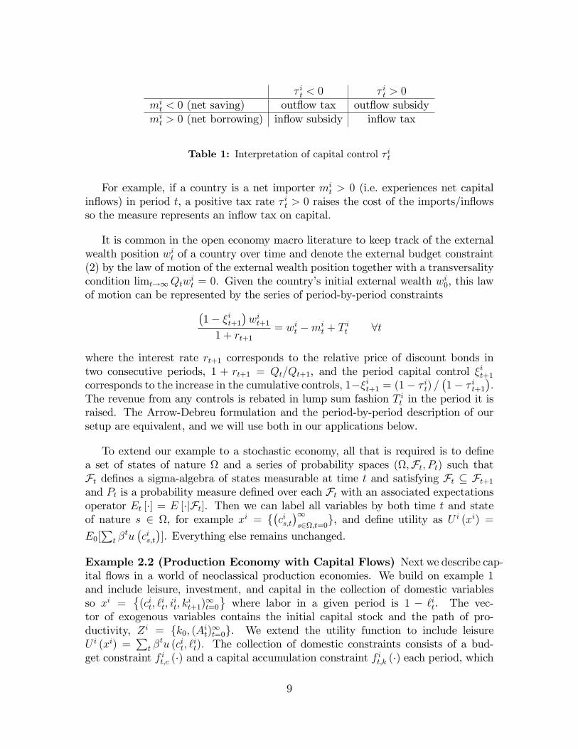
τ it < 0 τ it > 0mit < 0 (net saving) outflow tax outflow subsidy

mit > 0 (net borrowing) inflow subsidy inflow tax

Table 1: Interpretation of capital control τ it

For example, if a country is a net importer mit > 0 (i.e. experiences net capital

inflows) in period t, a positive tax rate τ it > 0 raises the cost of the imports/inflowsso the measure represents an inflow tax on capital.

It is common in the open economy macro literature to keep track of the externalwealth position wit of a country over time and denote the external budget constraint(2) by the law of motion of the external wealth position together with a transversalitycondition limt→∞Qtw

it = 0. Given the country’s initial external wealth wi0, this law

of motion can be represented by the series of period-by-period constraints(1− ξit+1

)wit+1

1 + rt+1

= wit −mit + T it ∀t

where the interest rate rt+1 corresponds to the relative price of discount bonds intwo consecutive periods, 1 + rt+1 = Qt/Qt+1, and the period capital control ξ

it+1

corresponds to the increase in the cumulative controls, 1−ξit+1 = (1− τ it) /(1− τ it+1

).

The revenue from any controls is rebated in lump sum fashion T it in the period it israised. The Arrow-Debreu formulation and the period-by-period description of oursetup are equivalent, and we will use both in our applications below.

To extend our example to a stochastic economy, all that is required is to definea set of states of nature Ω and a series of probability spaces (Ω,Ft, Pt) such thatFt defines a sigma-algebra of states measurable at time t and satisfying Ft ⊆ Ft+1

and Pt is a probability measure defined over each Ft with an associated expectationsoperator Et [·] = E [·|Ft]. Then we can label all variables by both time t and stateof nature s ∈ Ω, for example xi =

(cis,t)∞s∈Ω,t=0

, and define utility as U i (xi) =

E0[∑

t βtu(cis,t)]. Everything else remains unchanged.

Example 2.2 (Production Economy with Capital Flows) Next we describe cap-ital flows in a world of neoclassical production economies. We build on example 1and include leisure, investment, and capital in the collection of domestic variablesso xi =

(cit, `

it, i

it, k

it+1)∞t=0

where labor in a given period is 1 − `it. The vec-

tor of exogenous variables contains the initial capital stock and the path of pro-ductivity, Zi = k0, (A

it)∞t=0. We extend the utility function to include leisure

U i (xi) =∑

t βtu (cit, `

it). The collection of domestic constraints consists of a bud-

get constraint f it,c (·) and a capital accumulation constraint f it,k (·) each period, which

9

we denote by

f it,c (·) = cit + iit − Ait(kit)α (

1− `it)1−α −mi

t ≤ 0

f it,k (·) = kit+1 − (1− δ) kit − iit ≤ 0

As in example 1, mit equivalently captures net imports and capital inflows, and the

policy measure τ it can be interpreted as import taxes or as capital controls as in Table1. The framework can be extended to stochastic shocks as described before.

Example 2.3 (Multiple Consumption Goods) The framework of our previousexamples can also be extended in the direction of multiple consumption goods. Ex-panding on our baseline model in example 1, all that is required is to define thevariables cit, m

it, y

it and τ

it in each time period as vectors of size K capturing the

consumption, net imports, endowment and inflow taxes on each good k = 1...K inperiod t. Utility can then be written as U i (xi) =

∑t β

tu(cit,1, ..., c

it,K

). If some of the

consumption goods are non-traded, we omit them from the vector of net imports mit

so that dimmit = KT < K.

Assuming that τ it is a vector of equal size as mit supposes that the planner can

set differential tax/subsidy rates on each traded good k = 1...KT . Alternatively,assuming that the planner can only differentiate taxes by time period would amountto a restriction on the set of instruments τ it,1 = ... = τ it,KT

∀t. We will analyze suchrestrictions in Section 6.

3 Equilibrium

Definition 1 (Global Competitive Equilibrium) For given initial conditions (wi0, Zi)Ni=1,

an equilibrium in the described world economy consists of a set of feasible allocations(X i,M i, ζ i

)Ni=1

and external policy measures (τ i)Ni=1 together with a vector of world

market prices Q such that

• the individual allocations xi = X i and mi = M i solve the optimization prob-lem of private agents for given prices Q, aggregate allocations

(X i,M i, ζ i

)and

external policy measures (τ i),

• the aggregate allocations(X i,M i, ζ i

)and external policy measures (τ i) solve

the optimization problem of domestic policymakers for given prices Q and

• markets for international transactions clear∑N

i ωiM i = 0.

A formal description of the optimization problems of private agents and domesticpolicymakers is provided in appendix A.1.In the following two subsections, we separate the analysis of equilibrium in the

world economy into two steps. The first step is the domestic optimization problem

10

of each economy for a given external allocation (mi,M i) and is described in the nextsubsection. We show that the welfare of each country can be expressed as a reduced-form utility function V i (mi,M i) that greatly simplifies our analysis. The second stepsolves for the optimal external allocation of the economy given V i (mi,M i) for eachcountry and is described in the ensuing subsection. The section ends with a formallemma that the described two-step procedure solves the full optimization problem.

3.1 Domestic Optimization Problem

Domestic Agents We describe the domestic optimization problem of a represen-tative agent in country i for given external allocations (mi,M i), domestic aggregateallocations X i, domestic policy variables ζ i and exogenous state variables Zi. Forease of notation, we will suppress the vector Zi of exogenous state variables in thefunctions that we define in the following, though we note that all equilibrium objectsdepend on the exogenous vector Zi.We define the reduced-form utility of the representative agent as

vi(mi;M i, X i, ζ i

)= max

xiU i(xi)

s.t. f i(mi, xi,M i, X i, ζ i, Zi

)≤ 0 (5)

Denoting the shadow prices on the domestic constraints by the row vector λid whichcontains a shadow price for each element of the constraint set f i, the collection ofdomestic optimality conditions of a representative agent is

U ix = f ix

Tλid

T(6)

where Ux denotes a column vector of partial derivatives of the utility function withrespect to xi, and f ix is the Jacobian of derivatives of f

i with respect to xi and is amatrix of the size of f i (·) times the size of xi.

Domestic Policymaker For a given aggregate external allocation M i, a domesticpolicymaker in economy i chooses the optimal domestic policy measures ζ i and ag-gregate choice variables X i where she internalizes the consistency conditions xi = X i

and mi = M i as well as the implementability constraint (6). The planner’s problemis

maxXi,ζi,λid

U i(X i)

s.t. f i(M i, X i,M i, X i, ζ i, Zi

)≤ 0, (6) (7)

We assign the row vectors of shadow prices Λid to the collection of domestic constraints

f i and µid to the collection of domestic implementability constraints. The solutionto this problem defines the optimal domestic policy measures ζ i (M i) and aggregatedomestic choice variables X i (M i).

11

Optimal Domestic Allocation For a given aggregate external allocationM i, theoptimal domestic allocation in country i consists of a consistent domestic allocationxi = X i and domestic policy measures ζ i that solve the domestic optimization problem(7) of a domestic policymaker and, by implication, the domestic optimization problem(5) of private agents in country i since the policymaker observes the implementabilityconstraint (6).

Definition 2 (Reduced-Form Utility) We define the reduced-form utility func-tion of a representative agent in economy i for a given pair (mi,M i) by

V i(mi,M i

)= vi

(mi,M i, X i

(M i), ζ i(M i))

(8)

The reduced-form utility function V i (mi,M i) is also defined for off-equilibriumallocations in which mi and M i differ since individual agents are in principle free tochoose any allocation of mi, but in equilibrium, however, mi = M i will hold.

For the remainder of our analysis, we will focus on the case where the partialderivatives of this reduced-form utility function satisfy V i

m > 0 and V im + V i

M > 0∀i: ceteris paribus, a marginal increase in individual imports mi

t or a simultaneousmarginal increase in both individual and aggregate imports mi = M i increases thewelfare of a representative consumer. These are fairly mild assumptions that hold forthe vast majority of open economy macro models, including our baseline model.For concreteness, the reduced-form utility function in our baseline example 1 is

V i (mi,M i) =∑

t βtu (yit +mi

t), satisfying the above marginal utility conditions sinceV im,t = V i

m,t + V iM,t = βtu′ (cit) > 0∀i, t.

The reduced-form utility function V i (mi,M i) contains all the information that isrequired to describe external allocations and the global equilibrium.

3.2 External Allocations

Representative Agent Given the reduced-form utility function V i (mi,M i), aninternational price vector Q, a vector of tax instruments τ i on external transactions,initial external wealth wi0, transfer T

i and aggregate external allocations M i, thesecond-step optimization problem of a representative agent in country i defines theagent’s reduced-form import demand function

mi(Q, τ i, wi0, T

i,M i)

= arg maxmi

V i(mi,M i

)s.t. (2) (9)

Assigning the scalar shadow price λie to the external budget constraint (2), the asso-ciated optimality conditions (

1− τ i)TV im = λieQ

T (10)

12

describe the excess demand for each component of the import vector mi of the rep-resentative agent as a function of the vector of world market price Q, where the taxvector (1− τ i) pre-multiplies the column vector V i

m in an element-by-element fashion.We define the aggregate reduced-form import demand function M i (Q, τ i, wi0) as

the fixed point of the representative agent’s reduced-form import demand functionM i = mi

(Q, τ i, wi0,

τ iQ1−τ i ·M

i,M i)that satisfies the government budget constraint

T i = τ iQ1−τ i ·M

i. In some of our applications below, we will assume that wi0 = 0 andsuppress the last argument so the function is M i (Q, τ i).

Laissez-Faire Equilibrium We define the allocation that prevails when τ i = 0,T i = 0 ∀i as the laissez-faire equilibrium. We assume that domestic policymakers usetheir domestic policy instruments ζ i optimally as described in problem (7).

Competitive Planner Next we consider how a policymaker in country i optimallydetermines the policy instruments τ i on external transactions if she acts competitivelyon the world market in the sense of taking the price vector Q as given. We term thisinterchangably a competitive policymaker or competitive planner. There are severalpotential interpretations for such behavior: First, country i may be a small econ-omy with ωi ≈ 0 so that it is not possible for the planner to affect world marketprices. Secondly, the policymaker may choose her optimal allocations while actingwith benign neglect towards international markets. This may be the consequence ofan explicitly domestic objective of the policymaker prescribed by domestic law, be-cause the policymaker observes a multilateral agreement to abstain from monopolisticbehavior and disregard world-wide terms-of-trade effects, or because of enlightenedeconomics.7 We will analyze the behavior of a monopolistic policymaker who inter-nalizes her market power over world market prices Q in Section 5, which also discusseshow to distinguish between monopolistic and competitive behavior of policymakers.Since the planner has a full set of policy instruments to control M i, we can solve

directly for the planner’s optimal allocations and set the instruments τ i to implementthe desired allocation.A competitive planner who faces the reduced-form utility function V i (mi,M i)

and initial external wealth wi0 solves

maxM i

V i(M i,M i

)s.t. Q ·M i ≤ wi0 (11)

7For example, the US Federal Reserve claims to follow a policy of acting with benign neglecttowards external considerations such as exchange rates, as articulated by Bernanke (2013). Similarly,the G-7 Ministers and Governors proclaimed in a Statement after their March 2013 summit that “wereaffi rm that our fiscal and monetary policies have been and will remain oriented towards meetingour respective domestic objectives using domestic instruments, and that we will not target exchangerates”(G-7, 2013).

13

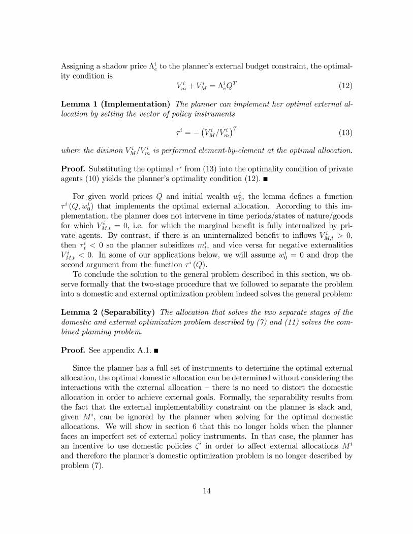
Assigning a shadow price Λie to the planner’s external budget constraint, the optimal-

ity condition isV im + V i

M = ΛieQ

T (12)

Lemma 1 (Implementation) The planner can implement her optimal external al-location by setting the vector of policy instruments

τ i = −(V iM/V

im

)T(13)

where the division V iM/V

im is performed element-by-element at the optimal allocation.

Proof. Substituting the optimal τ i from (13) into the optimality condition of privateagents (10) yields the planner’s optimality condition (12).

For given world prices Q and initial wealth wi0, the lemma defines a functionτ i (Q,wi0) that implements the optimal external allocation. According to this im-plementation, the planner does not intervene in time periods/states of nature/goodsfor which V i

M,t = 0, i.e. for which the marginal benefit is fully internalized by pri-vate agents. By contrast, if there is an uninternalized benefit to inflows V i

M,t > 0,then τ it < 0 so the planner subsidizes mi

t, and vice versa for negative externalitiesV iM,t < 0. In some of our applications below, we will assume wi0 = 0 and drop thesecond argument from the function τ i (Q).To conclude the solution to the general problem described in this section, we ob-

serve formally that the two-stage procedure that we followed to separate the probleminto a domestic and external optimization problem indeed solves the general problem:

Lemma 2 (Separability) The allocation that solves the two separate stages of thedomestic and external optimization problem described by (7) and (11) solves the com-bined planning problem.

Proof. See appendix A.1.

Since the planner has a full set of instruments to determine the optimal externalallocation, the optimal domestic allocation can be determined without considering theinteractions with the external allocation —there is no need to distort the domesticallocation in order to achieve external goals. Formally, the separability results fromthe fact that the external implementability constraint on the planner is slack and,given M i, can be ignored by the planner when solving for the optimal domesticallocations. We will show in section 6 that this no longer holds when the plannerfaces an imperfect set of external policy instruments. In that case, the planner hasan incentive to use domestic policies ζ i in order to affect external allocations M i

and therefore the planner’s domestic optimization problem is no longer described byproblem (7).

14

One practical implication of the lemma is that the two tasks of implementing theoptimal domestic and external allocations of the economy could be performed by twoseparate agencies, and the agency responsible for domestic policy does not need tocoordinate with the agency that sets the country’s external policy instruments.

Lemma 3 (Indeterminacy of Implementation) There is a continuum of alter-native implementations for the external allocation of a country i described by lemma 1,in which its policy instruments are re-scaled by a positive constant ki > 0 s.t. (1−τ i) =ki (1− τ i).

Proof. The re-scaling of policy instruments does not affect the external budgetconstraint of the economy since revenue is rebated lump-sum. It simply rescales theshadow price Λi

e in the optimality condition (12) by 1/ki. Therefore the old allocationstill satisfies all the optimality conditions of the economy.

The intuition is that the incentive of a representative agent to shift consumptionacross time/states of nature/goods only depends on the relative price of goods in thevector mi. Multiplying all prices by a constant and changing initial net worth by thecorresponding amount is equivalent to changing the numeraire.By the same token, if there exists a scalar hi ∈ (−1,∞) s.t. V i

M = hiV im, then it is

not necessary for the country i planner to intervene since the vector of policy instru-ments τ i = 0 will implement the same equilibrium as the vector τ i = − (V i

M/Vim)

T .This can easily be verified by setting ki = 1

1+hiand applying lemma 3. In the follow-

ing, we will assume that /∃hi that satisfies V iM = hiV i

m when we speak of a countrythat exhibits externalities.

3.3 Welfare Properties of Equilibrium

We now turn to the welfare properties of the described global equilibrium. We startwith a definition:

Definition 3 (Pareto Effi cient Allocations) A Pareto effi cient global allocationis a feasible global allocation

(M i, X i, ζ i

)Ni=1

such that there does not exist @ anotherfeasible allocation (M i, X i, ζ

i)Ni=1 that makes at least one country better off such that

U i(X) ≥ U i (X)∀i with at least one strict inequality.

Given this definition, we find:

Proposition 1 (Effi ciency of Global Equilibrium) The global competitive equi-librium allocation as per Definition 1 is Pareto effi cient.

15

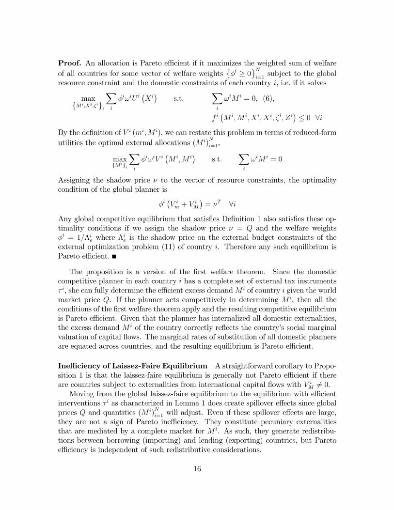
Proof. An allocation is Pareto effi cient if it maximizes the weighted sum of welfareof all countries for some vector of welfare weights

φi ≥ 0

Ni=1

subject to the globalresource constraint and the domestic constraints of each country i, i.e. if it solves

maxM i,Xi,ζi

i

∑i

φiωiU i(X i)

s.t.∑i

ωiM i = 0, (6),

f i(M i,M i, X i, X i, ζ i, Zi

)≤ 0 ∀i

By the definition of V i (mi,M i), we can restate this problem in terms of reduced-formutilities the optimal external allocations (M i)

Ni=1,

maxM ii

∑i

φiωiV i(M i,M i

)s.t.

∑i

ωiM i = 0

Assigning the shadow price ν to the vector of resource constraints, the optimalitycondition of the global planner is

φi(V im + V i

M

)= νT ∀i

Any global competitive equilibrium that satisfies Definition 1 also satisfies these op-timality conditions if we assign the shadow price ν = Q and the welfare weightsφi = 1/Λi

e where Λie is the shadow price on the external budget constraints of the

external optimization problem (11) of country i. Therefore any such equilibrium isPareto effi cient.

The proposition is a version of the first welfare theorem. Since the domesticcompetitive planner in each country i has a complete set of external tax instrumentsτ i, she can fully determine the effi cient excess demandM i of country i given the worldmarket price Q. If the planner acts competitively in determining M i, then all theconditions of the first welfare theorem apply and the resulting competitive equilibriumis Pareto effi cient. Given that the planner has internalized all domestic externalities,the excess demand M i of the country correctly reflects the country’s social marginalvaluation of capital flows. The marginal rates of substitution of all domestic plannersare equated across countries, and the resulting equilibrium is Pareto effi cient.

Ineffi ciency of Laissez-Faire Equilibrium A straightforward corollary to Propo-sition 1 is that the laissez-faire equilibrium is generally not Pareto effi cient if thereare countries subject to externalities from international capital flows with V i

M 6= 0.Moving from the global laissez-faire equilibrium to the equilibrium with effi cient

interventions τ i as characterized in Lemma 1 does create spillover effects since globalprices Q and quantities (M i)

Ni=1 will adjust. Even if these spillover effects are large,

they are not a sign of Pareto ineffi ciency. They constitute pecuniary externalitiesthat are mediated by a complete market for M i. As such, they generate redistribu-tions between borrowing (importing) and lending (exporting) countries, but Paretoeffi ciency is independent of such redistributive considerations.

16

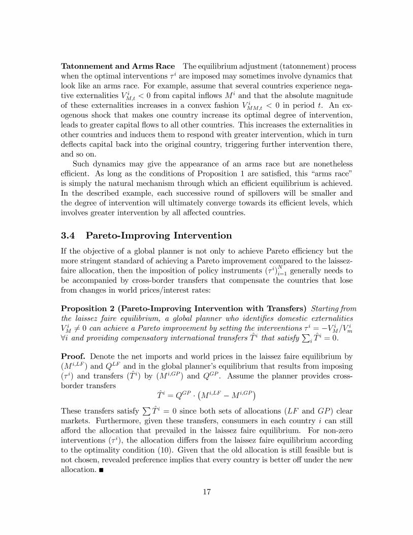
Tatonnement and Arms Race The equilibrium adjustment (tatonnement) processwhen the optimal interventions τ i are imposed may sometimes involve dynamics thatlook like an arms race. For example, assume that several countries experience nega-tive externalities V i

M,t < 0 from capital inflows M i and that the absolute magnitudeof these externalities increases in a convex fashion V i

MM,t < 0 in period t. An ex-ogenous shock that makes one country increase its optimal degree of intervention,leads to greater capital flows to all other countries. This increases the externalities inother countries and induces them to respond with greater intervention, which in turndeflects capital back into the original country, triggering further intervention there,and so on.Such dynamics may give the appearance of an arms race but are nonetheless

effi cient. As long as the conditions of Proposition 1 are satisfied, this “arms race”is simply the natural mechanism through which an effi cient equilibrium is achieved.In the described example, each successive round of spillovers will be smaller andthe degree of intervention will ultimately converge towards its effi cient levels, whichinvolves greater intervention by all affected countries.

3.4 Pareto-Improving Intervention

If the objective of a global planner is not only to achieve Pareto effi ciency but themore stringent standard of achieving a Pareto improvement compared to the laissez-faire allocation, then the imposition of policy instruments (τ i)

Ni=1 generally needs to

be accompanied by cross-border transfers that compensate the countries that losefrom changes in world prices/interest rates:

Proposition 2 (Pareto-Improving Intervention with Transfers) Starting fromthe laissez faire equilibrium, a global planner who identifies domestic externalitiesV iM 6= 0 can achieve a Pareto improvement by setting the interventions τ i = −V i

M/Vim

∀i and providing compensatory international transfers T i that satisfy∑

i Ti = 0.

Proof. Denote the net imports and world prices in the laissez faire equilibrium by(M i,LF ) and QLF and in the global planner’s equilibrium that results from imposing(τ i) and transfers (T i) by (M i,GP ) and QGP . Assume the planner provides cross-border transfers

T i = QGP ·(M i,LF −M i,GP

)These transfers satisfy

∑T i = 0 since both sets of allocations (LF and GP ) clear

markets. Furthermore, given these transfers, consumers in each country i can stillafford the allocation that prevailed in the laissez faire equilibrium. For non-zerointerventions (τ i), the allocation differs from the laissez faire equilibrium accordingto the optimality condition (10). Given that the old allocation is still feasible but isnot chosen, revealed preference implies that every country is better off under the newallocation.

17

In an international context, compensatory transfers may be diffi cult to implement.As an alternative, we show that a planner who can coordinate the policy instrumentsof both source and destination countries forM i can correct the domestic externalitiesof individual economies while holding world prices and interest rates constant so thatno wealth effects arise. As a result, the global planner’s intervention generates aglobal Pareto improvement at a first-order approximation.The following lemma demonstrates how a global planner can manipulate world

prices by simultaneously adjusting the instruments in all countries worldwide; thenwe show how this mechanism can be used to hold world prices fixed so as to avoidredistributive effects when correcting for externalities in a given country.

Lemma 4 Consider a global competitive equilibrium with an external allocation (M j)j,external policy instruments (τ j)j and world prices Q. A global planner can changeworld prices by dQ while keeping the external allocations of all countries constant bymoving the policy instruments in each country j = 1...N by moving(

dτ j)T

= −(M j

τ

)−1M j

Q (dQ)T (14)

Proof. We set the total differential of the net import demand functionM j(Q, τ j, wj0

)of country j with respect to world prices and policy instruments to zero,

dM j = M jQ (dQ)T +M j

τ

(dτ j)T

= 0

and rearrange to obtain equation (14).

In the following proposition, we assume an exogenous increase in the negativeexternalities dV i

M < 0 to a country i. If the country did not respond to this shock, itswelfare would decline by dV i

M ·M i. If the country responds by unilaterally increasingits policy instruments by dτ i = −dV i

M/Vim > 0 as suggested by lemma 1, world market

prices Q would change, and some countries would gain whereas others would lose fromthe resulting redistribution. The change in world prices and the redistribution canbe avoided using the following policy:

Proposition 3 (Pareto-Improving Intervention, No Transfers) Assume an ex-ogenous marginal increase in the externalities of country i that calls for an adjustmentdτ i in the optimal unilateral taxes. A global planner can correct for the increase inexternalities while keeping world prices constant dQ = 0 to avoid income and wealtheffects by adjusting (

dτ j)T

= −ωi(M i

τ

)−1M j

Q (MQ)−1M iτ

(dτ i)T

and(dτ it)T

=[I − ωi

(M i

τ

)−1M i

Q (MQ)−1M iτ

] (dτ i)T

where we define MQ ≡∑

j ωjM j

Q. In the resulting equilibrium, net imports (M j)j aremarginally altered but world prices are unchanged. By the envelope theorem, welfareis unchanged at a first-order approximation.

18

Proof. If the domestic planner implemented the unilaterally optimal change dτ i, thenworld prices would move by (dQ)T = −ωi (MQ)−1M i

τ (dτ i)T . According to Lemma

4, the move in world prices can be undone if the taxes of all countries j = 1...N aresimultaneously adjusted by − (M j

τ )−1M j

Q (dQ)T , which delivers the first equation ofthe proposition. The second equation is obtained by adding the optimal unilateralchange in intervention dτ i plus the adjustment given by the first equation with j =i. In the resulting equilibrium, the change in the externality dτ i is accounted forbut world market prices are unchanged. Furthermore, by the envelope theorem, thechange in welfare that results from a marginal change in M j is8

dV j∣∣dQ=0

=(V jm + V j

M

)T · dM j = 0

The intuition of this intervention is best captured by the following example:

Example 3.1 (Pareto-Improving Intervention, Symmetric Countries) Considera word economy that consists of N open economies as described in the baseline modelof example 2.1 that are identical except in their size ωi. Since the economies areidentical, observe thatM j

Q(MQ) = I ∀j. Assume country i experiences a marginal in-crease in some externality that calls for a change dτ i in its optimal unilateral externalpolicy instruments. A planner would achieve a Pareto improvement at a first-orderapproximation by instead setting

dτ i =(1− ωi

)dτ i

dτ j = ωidτ i

As this example illustrates, a planner who aims for a Pareto improving inter-vention would share the burden of adjusting policy instruments between country iand the rest-of-the-world according to their relative size. The larger country i, thegreater the impact of its interventions on world prices and therefore the more of theintervention the planner would shift to other countries so as to keep world prices Qconstant and avoid redistributions. In the extreme case that i is a small open econ-omy, the planner would only intervene in country i since its impact on world prices isnegligible. If the countries differ in other aspects than size, the terms M i

Q and Miτ in

proposition 3 account for their differential responses to changes in world prices andpolicy instruments.

8For non-infinitesimal changes in τ i, changes in net imports ∆M j have second-order effects onwelfare (i.e. effects that are negligible for infinitesimal changes but growing in the square of ∆M j)even if world prices are held constant. Under certain conditions, e.g. if there are only two typesof countries in the world economy, a global planner can undo these second-order effects via furtheradjustments in the world prices Q.

19

4 Examples and Applications

This section investigates several examples of externalities that have been used in theliterature and in policy circles to motivate policy interventions that affect externalallocations and that are therefore relevant for our analysis of spillover effects. Westart with two simple examples of learning externalities that are triggered either byexporting or by producing and in which capital account interventions represent first-best and second-best policy instruments, respectively. Then we analyze aggregatedemand externalities that may occur if a country experiences a liquidity trap.Even if one is skeptical of the existence of some of the described externalities,

these are important question to analyze since policymakers have explicitly invokedsuch externalities when they engaged in capital account interventions, exemplified byBrazilian finance minister Guido Mantega (see Wheatley and Garnham, 2010).

4.1 Learning-by-Exporting Externalities

Our first example, chosen for its simplicity of exposition, are learning-by-exportingexternalities.9 Assume a representative agent in a canonical open economy i thatbehaves as in our baseline model of capital flows (example 2.1), except that theendowment income yit+1 is a function ϕt (·) of the economy’s aggregate net importsM i

t that satisfies ϕt (0) = 0 and that is continuous and decreasing ϕ′t (Mt) ≤ 0 tocapture that higher net exports increase growth,

yit+1 = yit + ϕt(M i

t

)(15)

The reduced-form utility of a representative agent in country i is

V i(mi,M i

)=∑t

βtu

(yi0 +

t−1∑s=0

ϕs(M i

s

)+mi

t

)with marginal utility of private and aggregate capital inflows of V i

m,t = βtu′ (Cit) and

V iM,t = ϕ′t (M i

t ) βtvt+1 where vit+1 =

∑∞s=t+1 β

s−tu′ (Cis) is the PDV of one extra unit of

output growth at time t+ 1, capturing the growth externalities from exporting. Fol-lowing lemma 1, a planner can implement the socially effi cient allocation in economyi by imposing capital controls

τ it = −V iM,t/V

im,t = −

ϕ′t (M it ) v

it+1

u′ (Cit)

≥ 0 (16)

9There is a considerable theoretical literature that postulates that such effects are important fordeveloping countries in the phase of industrialization. See for example Rodrik (2008) and Korinekand Servén (2010). In the empirical literature there have been some studies that document theexistence of learning externalities, whereas others are more skeptical. For a survey see e.g. Giles andWilliams (2000).

20

The planner subsidizes exports/capital outflows and taxes imports/capital inflows inperiods in which net exports generate positive externalities.It is typically argued that learning externalities are only relevant during transition

periods in developing economies (see e.g. Rodrik, 2008). In that case, the externalityterm ϕ′t (M i

t ) would at first be negative and would gradually converge to zero.In the described framework, capital control are the first-best policy tool to inter-

nalize learning-by-exporting externalities, since they directly target net saving andhence the trade balance of the economy.Since our model of learning-by-exporting externalities nests into the general model

of section 2, it is a straightforward application of proposition 1 that the interventionof a competitive planner to internalize such externalities leads to a Pareto effi cientoutcome from a global perspective.

4.2 Learning-by-Doing Externalities

Capital account intervention may also serve as a second-best instrument in an econ-omy where it would be desirable to use domestic policy measures to correct a distor-tion but such measures are not available.The following example show how capital controls may serve to internalize learning-

by-doing externalities in a production economy in which productivity growth is anincreasing function of employment. The first-best policy instrument in such a settingis a subsidy to employment. However, if such an instrument is not available (forexample, because of a lack of fiscal resources, a large informal sector, or the risk ofcorruption), it may be optimal to resort to capital controls as a second-best instrumentto improve welfare.Assume that the output of a representative worker in economy i is given by yit =

Ait`it, where labor `

it imposes a convex disutility d (`it) on workers. We capture learning-

by-doing externalities by assuming that productivity growth Ait in the economy is acontinuous and increasing function of aggregate employment ψt (Lit) that satisfiesψ′t (·) ≥ 0 so that

Ait+1 = Ait + ψt(Lit)

= Ai0 +t∑

s=0

ψs(Lis)

(17)

In the described economy, the first-best policy instrument to internalize suchlearning effects would be a subsidy sit to wage earnings in the amount of s

it =

ψ′t (Lit) vA,t+1/[u′ (cit)A

it] where vA,t+1 =

∑∞s=t+1 β

s−tu′ (cis)Lis is the PDV of one unit

of productivity growth starting period t+ 1.In the absence of a policy instrument to target the labor wedge, a planner faces

the implementability constraint

Aitu′ (AitLit +M i

t

)= d′

(Lit)

(18)

which reflects the optimal labor supply condition of individual workers. Observe thatreducing M i

t in this constraint is akin to a negative wealth effect and increases the

21

marginal utility of consumption, which in turn serves as a second-best instrument toraise Lit and trigger learning-by-doing externalities.Accounting for this implementability constraint and imposing the consistency con-

dition `it = Lit, a constrained planner recognizes that the reduced-form utility of theeconomy is

V(mi,M i

)= max

Lit

∑t

βtu(AitL

it +mi

t

)− d

(Lit)

s.t. (17), (18)

with marginal utility of private and aggregate capital inflows of V im,t = βtu′ (Ci

t) andV iM,t = −λitβtAitu′′ (Ci

t) < 0 where λt is the shadow price on the implementabilityconstraint (18) and is given by

λit =ψ′t (Lit) v

iA,t+1

d′′ (Lit)− (Ait)2u′′ (Ci

t)> 0

In this expression, the positive learning externalities (in the numerator) are scaled bya term that reflects how strongly labor supply responds to changes in consumption(in the denominator).10 If the economy has outgrown its learning externalities, theterm drops to zero.Following lemma 1, the planner can implement this second-best solution by im-

posing capital controls of11

τ it = −λtAitu′′ (Ci

t)

u′ (Cit)

=ψ′t (Lit) vA,t+1

d′ (Lit)(

1 + ηLσC

) (19)

This control reduces capital inflows and stimulates domestic production to bene-fit from greater learning-by-doing externalities. The numerator in the expression isanalogous to the optimal capital control (16) under learning-by-exporting. In the

10Given that there are no first-best policy instruments available, the PDV of one unit of produc-tivity growth νiA,t also includes the effects of higher productivity on future labor supply decisions:on the one hand, higher productivity increases incentives to work, on the other hand it makes theagent richer and reduces the incentive to work via a wealth effect. The two effects are captured bythe two expressions in square brackets,

viA,t+1 =

∞∑s=t+1

βs−tu′(Cis)Lis + λis

[u′(Cis)

+Aisu′′ (Cis)Lis]

11The right-hand side of the expression can be obtained by substituting for λit and observing thatAitu

′ (Cit) = d′(Lit)and

Aitu′′ (Cit)

d′′(Lit)−(Ait)2u′′(Cit) = − 1

Ait

(1 + ηL

σC

)

22

denominator term, ηL and σC are the Frisch elasticity of labor supply and the in-tertemporal elasticity of substitution: the second-best intervention is more desirablethe more responsive the marginal disutility of labor (high ηL) and the more responsivethe marginal utility of consumption (low σC).Proposition 1 implies, as in the previous case, that the application of second-best

capital controls lead to a globally Pareto effi cient outcome. Even though capitalcontrols (19) are only second-best instruments, they are chosen to precisely equatethe marginal social benefit from indirectly triggering the LBD-externality to theirmarginal social cost, given the restriction on the set of available instruments. Re-ducing domestic consumption by running a trade surplus is the only way available toinduce domestic agents to work harder. Since a global planner does not have supe-rior instruments, he cannot do better than this and chooses an identical allocation.The global effi ciency implications of second-best capital controls are no different fromother reasons to implement capital controls.

4.3 Aggregate Demand Externalities at the ZLB

Next we study the multilateral implications of capital controls to counter aggregatedemand externalities at the zero lower bound (ZLB) on nominal interest rates. Wedevelop a stylized framework that captures the essential nature of such externalitiesin the spirit of Krugman (1998) and Eggertsson and Woodford (2003), adapted to anopen economy framework as in Jeanne (2009).12

Assume that a representative consumer in country i derives utility from consumingcit units of a composite final good and experiences disutility from providing `it unitsof labor. Collecting the two time series in the vectors ci and `i, we denote

U i(ci, `i

)=∑

βt[u(cit)− d

(`it)]

As is common in the New Keynesian literature, we assume that there is a con-tinuum z ∈ [0, 1] of monopolistic intermediate goods producers who are collectivelyowned by consumers and who each hire labor to produce an intermediate good of va-riety z according to the linear function yizt = `izt , where labor market clearing requires∫`izt dz = `it. All the varieties are combined in a CES production function to produce

final output

yit =

(∫ 1

0

(yizt) ε−1

ε dz

) εε−1

where the elasticity of substitution is ε > 1. We assume that the monopoly wedgearising from monopolistic competition is corrected by a proportional subsidy 1

ε−1that

is financed by a lump-sum tax on producers. This implies that the wage income

12A complementary analysis of prudential (as opposed to stimulative) capital controls due toaggregate demand externalities at the ZLB is provided in Section 5.2 of Farhi and Werning (2013)in a small open economy setting.

23

and profits of the representative agent equal final output, which in turn equals laborsupply wt`it + πit = yit = `it. In real terms and vector notation, the period budgetconstraints of a representative agent and the external budget constraint are given by

ci = w`i + πi +mi = yi +mi andQ

1− τ i ·mi − T i ≤ wi0

The condition for the optimal labor supply of the representative agent is

d′(`it)

= witu′(cit)

We assume that the nominal price of one unit of consumption good follows anexogenous path P i = (1, P i

2, Pi3, ...) that is credibly enforced by a central bank (see

Korinek and Simsek, 2014, for further motivation). This assumption precludes thecentral bank from committing to a future monetary expansion or future inflation inorder to stimulate output in the present period.13 The corresponding gross rate ofinflation is given by Πi

t+1 = P it+1/P

it or by Πi = P/L (P ) in vector notation with lag

operater L (·). One example is a fixed inflation target Πit+1 = Πi ∀ t.

Combining the ZLB constraint on the nominal interest rate iit+1 = Rt+1Πt+1−1 ≥ 0with the aggregate Euler equation to substitute for Rt+1, the ZLB in period t imposesa ceiling on aggregate period t consumption,

u′(Cit

)≥ β

Πit+1

u′(Cit+1

)∀t (20)

Intuitively, a binding ZLB implies that consumption is too expensive in period t com-pared to consumption in the following period, limiting aggregate demand in period tto the level indicated by the constraint.In the laissez-faire equilibrium, this constraint is satisfied with strict inequality

if world aggregate demand for bonds and by extension the world interest rate issuffi ciently high, i.e. if Rt+1 ≥ 1/Πi

t+1. Then the market-clearing wage Wit = 1 will

prevail and output Y it is at its effi cient level determined by the optimality condition

u′ (Cit) = d′ (Lit). We call this output level potential output Y

i∗t .

If worldwide aggregate demand declines and the world real interest rate hits thethreshold Rt+1 = 1/Πi

t+1, then the domestic interest rate cannot fall any further.Instead, any increase in the world supply of bonds will flow to economy i, which paysa real return of 1/Πi

t+1 by the feature of offering liabilities with zero nominal interestrate. Given the high return on nominal bonds, consumers in economy i find thattoday’s consumption goods are too expensive compared to tomorrow’s consumptiongoods and consumers reduce their demand for today’s consumption goods. Output isdemand-determined, so Y i

t falls below potential output Yi∗t in order to satisfy equation

13It is well known in the New Keynesian literature that the problems associated with the zerolower bound could be avoided if the monetary authority was able to commit to a higher inflationrate. See e.g. Eggertsson and Woodford (2003).

24

(20). The wage also falls below its effi cient level W it < 1. This situation captures the

essential characteristic of a liquidity trap: at the prevailing nominal interest rate ofzero, consumers do not have suffi cient demand to absorb both domestic output andthe capital inflowM i

t . Intermediate producers cannot reduce their prices and need toadjust output so that demand equals supply.At the ZLB, a planner finds it optimal to erect barriers against capital inflows

or encourage capital outflows in order to stimulate domestic aggregate demand. Wesubstitute the domestic period budget constraint and the consistency condition xi =X i and denote the reduced-form utility maximization problem of a planner in countryi according to definition 2 by

V(mi,M i

)= max

Li

∑βt[u(Lit +mi

t

)− d

(Lit)]

s.t. u′(Lit +M i

t

)≥ β

Πit+1

u′(Lit+1 +M i

t+1

)∀t

d′(Lit)≤ u′

(Lit +M i

t

)∀t

where the second line captures the implementability constraint that ensures thatthe central bank cannot commit to future monetary expansion to induce workers toproduce more, as we assumed earlier.Assigning the shadow prices βtµt and β

tγt to the two constraints, the associatedoptimality conditions are

FOC(Lit)

: u′(Cit

)− d′

(Lit)

+[µt − µt−1/Π

it

]u′′(Cit

)− γt

[d′′(Lit)− u′′

(Cit

)]= 0

When the ZLB constraint is loose, the shadow prices µt and γt are zero. If the

ZLB is binding in period t, then µt =u′(Cit)−d′(Lit)−u′′(Cit)

> 0 reflects the labor wedge in

the economy created by the lack of demand and the second constraint is triviallysatisfied so γt = 0. If the ZLB is loose in the ensuing period t + 1, then the plannerwould like to commit to stimulate output in that period as captured by the term−µtu′′

(Cit+1

)/Πi

t+1 so as to relax the ZLB constraint at date t, but we imposed thesecond constraint to reflect that the planner cannot commit to do this. Thereforeu′(Cit+1

)= d′

(Lit+1

)in that period and the shadow price γt+1 adjusts so that the

optimality condition is satisfied γt+1 =−µtu′′(Cit+1)/Πi

t+1

d′′(Lit+1)−u′′(Cit+1)> 0.

The externalities of capital inflows in periods t and t+ 1 in such an economy aregiven by the partial derivatives

Vm,t (·) = βtu′(Cit

)VM,t (·) = βt

[µt − µt−1/Π

it + γt

]u′′(Cit

)If the economy experiences a liquidity trap in period t but has left the trap in periodt + 1, then VM,t = βtµtu

′′ (Cit) = −βt [u′ (Ci

t)− d′ (Lit)] < 0 —the externality from aunit capital inflow is to reduce aggregate demand by one unit, which wastes valuableproduction opportunities as captured by the positive labor wedge u′ (Ci

t)− d′ (Lit). It

25

is optimal to set the policy instrument τ it = 1− d′(Lit)u′(Cit)

> 0 precisely such as to reflect

this social cost, thereby restricting capital inflows and encouraging outflows.In the following period, it is beneficial to commit to setting τ it+1 < 0 so as to

restrict capital outflows or subsidize capital inflows since

VM,t+1 = −βt+1µt/Πit+1

[d′′(Lit+1

)d′′(Lit+1

)− u′′

(Cit+1

)]u′′ (Cit+1

)> 0

This has the effect of raising future consumption, which stimulates consumption dur-ing the liquidity trap by relaxing the ZLB constraint (20).14

Note that the capital account interventions of a planner in this setting are second-best policies since the first-best policy would be to restore domestic price flexibilityto abolish the ZLB constraint. The planner solves the optimal trade-off betweenforegoing effi cient consumption smoothing opportunities by trading with foreignersand wasting profitable production opportunities because of the ZLB.

4.4 Exchange Rate Intervention

[To be written up.]

4.5 Level of Fiscal Spending

Our findings also apply to multilateral considerations about the optimal level of fiscalspending. Such considerations have, for example, been at the center of the politicaldebate on coordinating fiscal stimulus in the aftermath of the Great Recession (see e.g.the G-20 Leaders’Declaration, Nov. 2008; Spilimbergo et al., 2008). We demonstratehow uncoordinated fiscal policy decisions lead to an effi cient equilibrium as longas the three conditions underlying our general effi ciency proposition are met. Inthe context of fiscal policy, the most important condition is price-taking behaviorsince fiscal spending has important terms-of-trade effects. If national policymakersconsider these terms-of-trade effects in their optimal policy-making, they are exertingmonopoly power and implementing an ineffi cient level of fiscal spending. The ensuingexample will be followed by a more detailed discussion of monopolistic behavior inSection 5.

[To be completed.]

14In a time-consistent setting for capital account interventions, the planner would not be able tocommit to future policy actions. The intervention during a liquidity trap would still be given by thesame expression VM,t = d′

(Lit)− u′

(Cit), but after the liquidity trap has passed the planner would

find VM,t+1 = 0 and no further intervention would occur.

26

5 Monopolistic Behavior

5.1 Optimization Problem

Assume next that there is a monopolistic planner in country i with positive mass ωi >0 that maximizes the utility of the representative consumer U i and internalizes thatshe has market power over world prices Q. We solve the problem of the monopolisticplanner under the assumption that the remaining countries j 6= i behave accordingto the competitive planning setup in section 3.2. The excess demand of the rest-of-the-world excluding country i is then given by the function15

M−i (Q) =∑j 6=i

ωjM j(Q, τ j (Q)

)The function can be inverted to obtain an inverse rest-of-the-world excess demandfunction Q−i(M−i).A monopolistic planner recognizes that global market clearing requires ωiM i +

M−i (Q) = 0 and that her external allocations M i affect world prices since Q =Q−i (−ωiM i). She solves the optimization problem

maxM i

V i(M i,M i

)s.t. Q−i(−ωiM i) ·M i ≤ wi0

leading to the optimality conditions

V im + V i

M = ΛieQ

T(1− E iQ,M

)with E iQ,M = ωiQ−iM

(M i/QT

)(21)

where the column vector E iQ,M represents the inverse demand elasticity of imports ofthe rest of the world and consists of four elements: the country weight ωi reflectsthe country’s market power in the world market; the Jacobian square matrix Q−iM =∂Q−i/∂M−i captures how much world market prices respond to absorb an additionalunit of exports from country i. The column vector M i post-multiplies this matrixto sum up the marginal revenue accruing to country i from the different goods as aresult of monopolistically distorting each good, where the vector M i is normalizedelement-by-element by the price vector Q to obtain elasticities.

Lemma 5 (Monopolistic Capital Account Intervention) The allocation of themonopolistic planner who internalizes her country’s market power over world pricescan be implemented by setting the vector of external policy instruments to

1− τ i =1 + V i

M/Vim

1− E iQ,M(22)

where all divisions are performed element-by-element.15Our findings can easily generalized to the case where other countries engage in monopolistic

behavior or operate under laissez-faire. The only important assumption for our problem is thateach country j has a well-defined and continuous demand function. This rules out, for example,discontinuous trigger strategies.

27

Proof. The tax vector τ i ensures that the private optimality condition of consumers(10) replicates the planner’s Euler equation (21).

Returning to equation (21), a monopolistic planner equates the social marginalbenefit of imports V i

m + V iM to the marginal expenditure QT

(1− E iQ,M

)rather than

to the world price QT times a factor of proportionality Λie. She intervenes up to the

point where the marginal benefit of manipulating world prices —captured by the elas-ticity term Λi

eQTE iQ,M —equals the marginal cost of giving up profitable consumption

opportunities ΛieQ

T − (V im + V i

M). However, giving up profitable consumption op-portunities creates a deadweight loss —the planner introduces a distortion to extractmonopoly rents from the rest of the global economy. The intervention constitutes aclassic ineffi cient beggar-thy-neighbor policy:

Proposition 4 (Ineffi ciency of Exerting Market Power) An equilibrium in whicha domestic planner in a country with ωi > 0 exerts market power is Pareto-ineffi cient.

Proof. The result is a straightforward application of proposition 1 that optimalityrequires competitive behavior.

To provide some intuition, assume that the matrix Q−iM in a country with ωi > 0is a diagonal matrix and that there are no domestic externalities so V i

M = 0.16 Thediagonal entries, indexed by t, satisfy ∂Q−it /∂M

−it < 0, reflecting that greater rest-

of-the-world imports M−it of good t require a lower world price Qt. If the country

is a net importer M it > 0 of good t then the elasticity E iQ,M,t is negative and the

optimal monopolistic tax on imports τ it > 0 is positive. Similarly, for goods that arenet exports M i

t < 0 the planner reduces the quantity exported by a tax τ it < 0. Thiscaptures the standard trade-reducing effects of monopolistic interventions.

5.2 Distinguishing Competitive and Monopolistic Behavior

The spillover effects of a policy intervention in external allocations are the same, nomatter what the motive for intervention. However, the effects on Pareto effi ciencyand thus the scope for global cooperation depend crucially on whether policymakerscorrect for domestic distortions (as described in lemma 1) or exert market power (asdescribed in lemma 5).Unfortunately there is no general recipe for distinguishing between the two mo-

tives for intervention. It is easy for policymakers to invoke market imperfections,domestic objectives or different political preferences to justify an arbitrary set ofpolicy interventions in the name of domestic effi ciency, and it is diffi cult for the in-ternational community to disprove them. Specifically, for any reduced-form utilityfunction V i(mi,M i) and monopolistic interventions τ i, there exists an alternative

16This is the case, for example, if the reduced-form utility V(mi,M i

)is Cobb-Douglas in mi.

28

reduced-form utility function V i(mi,M i) such that τ i implements the optimal com-petitive planner allocation under that utility function,

V i(mi,M i) = V i(mi,M i)− τ i ·(V imM

i)

The reduced-form utility function V i(·) can in turn be interpreted as deriving from afundamental utility function U i (xi) and a set of constraints f i (·) that justify it.Nonetheless, the direction of optimal monopolistic policy interventions is often in-

structive to determine whether it is plausible that a given intervention is for domesticor monopolistic reasons. In the following, we describe optimal monopolistic capitalaccount interventions along a number of dimensions. If the observed interventions ofa policymaker are inconsistent with these observations, then they are likely not formonopolistic reasons. Recall the definition of the elasticity E iQ,M = −ωiQ−iM (M i/Q)

T ,and let us discuss the various parameters:

Country Size ωi The optimal monopolistic intervention is directly proportional tothe country’s weight ωi in the world economy. Larger countries have a greaterimpact on the rest of the world since market clearing requires M−i = ωiM i.For example, if a small open economy with ωi ≈ 0 and undifferentiated exportsregulates capital in- or outflows, the reason cannot be monopolistic.

Responsiveness of Price Q−iM Monopolistic intervention requires that world mar-ket prices are suffi ciently responsive to changes in consumption. If there are,for example, close substitutes to the goods traded by country i, this is unlikelyto be the case.

Direction and Magnitude of Flows M i The intervention to manipulate a givenprice Qt is directly proportional to the magnitude of a country’s net importsM i

t in that time period/good/state of nature. The larger Mit in absolute value,

the greater the revenue benefits from distorting the price Qt. By contrast, ifM i

t ≈ 0, the optimal monopolistic intervention is zero.

The direction and magnitude of flows has the following implications for monop-olistic behavior:

• Intertemporal trade: In our example 2.1 with a single consumptiongood per time period, the elements of M i capture net capital flows orequivalently the trade balance. In time periods in which the trade balanceis close to zeroM i

t ≈ 0, it is impossible to distort intertemporal prices. Bycontrast, monopolistic reasons may be involved if a country with a largedeficit M i

t > 0 taxes inflows τ it > 0 to keep world interest rates lower, orvice versa for a country with a large surplus M i

t < 0. If capital accounts

29

are closed to private agents, optimal monopolistic intervention consists ofreduced/increased foreign reserve accumulation.17

• Risk-sharing: In the stochastic extension of example 2.1, M it (st) denotes

different states of nature. Each country has —by definition —monopolypower over its own idiosyncratic risk. Optimal risk-sharing implies greaterinflows (imports) in bad states and greater exports in good states of nature.A planner who exerts monopoly power would restrict risk-sharing so as toobtain a higher price for the country’s idiosyncratic risk and to reducethe price of insurance from abroad. By contrast, if a country encouragesinsurance (e.g. by encouraging FDI and forbidding foreign currency debt;see Korinek, 2010), then the motive is unlikely to be monopolistic.

• Intratemporal trade: Exercising monopoly power in intratemporal tradeconsists of tariffs τ it,k > 0 on imported goods k withM i

t,k > 0 and taxes onexports τ it,k < 0 for M i

t,k < 0, as is well known from a long literature ontrade policy (see e.g. Bagwell and Staiger, 2002).

In all these cases, observe that the optimal monopolistic intervention typicallyreduces the magnitude of capital or goods flows but does not change theirdirection.

It is straightforward that any price intervention τ i can also be implemented byan equivalent quantity restriction M i, for example by imposing a quota rather thana tax on inflows.

5.3 Monopolistic Use of Domestic Policy Instruments

A policymaker can also use domestic policies ζ i to monopolistically distort her coun-try’s terms of trade. This may be desirable if she faces restrictions on the set ofexternal policy instruments, for example due to international agreements or due totechnical diffi culties in targeting or implementing capital controls. If the set of exter-nal policy instruments τ i is complete, then it would be suboptimal to distort domesticpolicies for monopolistic reasons and only external instruments are used for this pur-pose:

Lemma 6 A monopolistic planner who has a complete set of external instruments τ i

will not distort domestic policies ζ i to exert market power.

17For example, when policymakers reduce reserve accumulation because they are concerned thatthey are pushing down the world interest rate too much, this is classic non-competitive behaviorand is equivalent to monopolistic capital controls. This corresponds to statements by some Chinesepolicymakers that were concerned about pushing down US Treasury yields because of their reserveaccumulation.

30

Proof. The proof follows from the separability result in appendix A.1. In particular,observe that the implementability constraint on external transactions is slack whenthe planner has complete instruments and therefore µie = 0. As a result, the optimalitycondition for domestic instruments ζ i is unchanged.

To illustrate how domestic policy instruments are used for monopolistic reasons,we consider the extreme case of a monopolistic planner who cannot use externalpolicy instruments at all so τ i = 0.18 Furthermore, for simplicity, assume that theplanner faces no domestic targeting problems so that she can choose X i without anyrestrictions. This allows us to ignore the domestic optimization problem of privateagents and treat the vectorX i as part of the vector of policy instruments ζ i = X i, ζ

ifor ease of notation. A monopolistic planner under these assumptions solves

maxM i,ζi,λie

U i(ζ i) s.t. f i(M i,M i, ζ i) ≤ 0,

Q−i(−ωiM i

)·M i ≤ wi0,

λidfim = −λieQ−i

(−ωiM i

)The domestic constraint and external budget constraint in the first two lines are theusual ones, but the planner internalizes the effects of her external allocations on worldmarket prices Q−i (−ωiM i). The implementability constraints in the third line reflectthat the planner lacks policy instruments to create a wedge in the external optimalitycondition of private agents. We assign the usual shadow prices Λi

d, Λie and µ

ie to these

constraints and obtain the optimality conditions

FOC(M i)

: 0 = Λidf

im+M + Λi

eQ(1− ωiE−iQ,M

)+ µie

[λidf

im(m+M) − ωiλieQ−iM

]FOC

(ζ i)

: U iζ = Λi

dfiζ + µie

(λidf

imζ

)FOC

(λie)

: 0 = µie ·QT

where we denote the sum of partial derivatives as fm+M = ∂f∂m

+ ∂f∂M

and so on tocondense notation. The optimality condition on λie implies that the price-weightedsum of shadow prices on the external implementability constraint (IC) is zero so∑

k µie,kQk = 0. With the exception of knife-edge cases (e.g. no monopoly power

because ωi = 0), some of the shadow prices on the external IC will therefore bepositive and some will be negative. In particular, if we collect the first two terms inthe optimality condition on M i in the vector −V i

m+M , we can write the condition as

µie = A−1[V im+M − Λi

eQ(1− ωiE−iQ,M

)]where A = λidf

im(m+M) − ωiλieQ

−iM is a negative semidefinite matrix. To interpret

this expression, consider an A that is close to diagonal and assume that there are no18We could also place a more general set of restrictions on the set of policy instruments, e.g.

Ξ(τ i)≤ 0. Our main insight that a monopolistic planner would use domestic policy instruments to

distort external allocations would continue to hold.

31

domestic externalities so V im = V i

m+M .19 In the absence of monopolistic behavior, the

square brackets in this expression would be zero by the private optimality condition ofconsumers V i

m = λieQ. By contrast, for a monopolistic planner, the vector of shadowprices µie captures the monopolistic cost (benefit) of increasing imports of each goodand is therefore negative for net imports and positive for net exports.In setting the optimal domestic allocation and policy measures ζ i according to

FOC(ζ i), the planner internalizes that the marginal domestic cost of consumption

or policy measures Λidf

iζ needs to be complemented by the monopolistic benefits or

costs.

Example: [fiscal policy/fiscal stimulus —to be completed]

6 Imperfect External Policy Instruments

In practice policymakers do not have the set of perfect external policy instrumentsthat we have depicted in our earlier analysis (see e.g. Carvalho and Marcio, 2006,in the context of capital controls). This section analyzes under what circumstancesimperfections in the set of policy instruments create a case for global policy coordi-nation. We first discuss circumstances under which the set of policy instruments iseffectively complete even if there are limitations on actual instruments. Then we an-alyze two types of such imperfections: implementation costs and imperfect targeting.We formalize both and analyze when and how a global planner can achieve a Paretoimprovement by coordinating the imperfect policy instruments of different countries.

6.1 Completeness of Set of External Instruments

Definitions A policymaker in country i has a complete set of external policy in-struments τ i if the policymaker has suffi cient instruments to implement any feasibleexternal allocation as a decentralized allocation, i.e. ∀M i s.t. Q ·M i = wi0, ∃τ i s.t.M i = M i (Q, τ i, wi0). In the baseline setup of section 2, the set of policy instrumentsis complete by construction.Conversely, a policymaker in country i has an incomplete set of external pol-

icy instruments τ i if there are feasible external allocations that the planner cannotimplement as a decentralized allocation, i.e. ∃M i with Q · M i = wi0 s.t. /∃τ i s.t.M i = M i (Q, τ i, wi0). Clearly, the two definitions are exhaustive and mutually exclu-sive, i.e. every set of external policy instruments is either complete or incomplete.

19This assumption holds exactly if mi enters in Cobb-Douglas fashion. In the general case, thediagonal elements of the matrix are likely to be an order of magnitude larger than the off-diagonalelements as long as goods aren’t strong complements or substitutes.

32

A policymaker in country i has an effectively complete set of external policy in-struments τ i if the policymaker has suffi cient instruments to implement the optimalallocation that she would choose if she had a complete set of external instruments, i.e.∃τ i s.t. M i (Q, τ i, wi0) = arg maxM i V (M i,M i) s.t. Q ·M i = wi0. If a policymaker’sset of external instruments is complete, it is also effectively complete, but not viceversa — it is possible that the planner has suffi cient instruments to implement theoptimal allocation but not all other feasible allocations.

Effective Completeness and Effi ciency Our effi ciency result in proposition 1requires that the policymakers in each country have at least an effectively complete setof external policy instruments. In that case, each policymaker can choose her desiredallocations, and the logic of the first welfare theorem applies. Observe that onlyeffective completeness in external instruments is required. No matter how incompletethe set of domestic policy instruments is, our effi ciency proposition holds since aglobal planner cannot improve on the allocation given the restrictions on domesticinstruments.The case V i

M = 0 of no externalities in international transactions represents abenchmark case in which the set of instruments of the policymaker in country i is al-ways effectively complete. In that case, incompleteness in actual policy instruments isirrelevant since the laissez faire external allocation implements the effi cient allocation.

Effective Completeness at the Global Level The set of external policy in-struments (τ i)

Ni=1 is effectively complete at the global level if a global planner can

implement a Pareto effi cient equilibrium for a given set of welfare weights. A givenset (τ i)

Ni=1 may be effectively complete at the global level even if the set of policy

instruments τ i in some country i is not effectively complete. In that case a globalplanner can implement a Pareto effi cient equilibrium that is unattainable withoutglobal cooperation. Effective completeness at the global level is thus a weaker con-dition than effective completeness in each country i. The reason for the discrepancybetween the two concepts is captured by lemma 3: there is a continuum of waysof implementing a given global allocation, but only one of these implementationscorresponds to a global competitive equilibrium in which national policymakers actunilaterally. A global planner may be able to employ one of the other implementationsif the implementation through a competitive equilibrium is unavailable.

Example 6.1 (Effectively Complete Instruments at the Global Level) Considera world economy with N = 2 countries that are described by the reduced-form utilityfunctions V i (mi,M i). Assume that country 1 suffers from externalities to capitalinflows so V 1

M 6= 0 but does not have any policy instruments to correct for them.Furthermore, assume that country 2 does not suffer from externalities V 2

M ≡ 0 buthas a complete set of external instruments τ 2.

33

If country 1 had the instruments to do so, it would impose an optimal tax oncapital inflows τ 1∗

0 = − (V 1M/V

1m)

T . However, since the country has no policy instru-ments, the global competitive equilibrium coincides with the laissez-faire equilibrium—country 2 has no incentive to intervene in its external transactions.By contrast, under cooperation, country 2 would set its policy instrument 1−τ 2

0 =1

1−τ1∗0, i.e. it would tax capital outflows to correct for the negative externalities of

inflows in country 1 and implement a Pareto effi cient allocation.

6.2 Imperfections in Set of External Instruments

To formally capture imperfections in the set of instruments of a policymaker in countryi, we assume that there is a cost to imposing the set of policy instruments τ i given bya function Γi (τ i) that is non-negative, satisfies Γi (0) = 0, is convex and continuouslydifferentiable, and that negatively enters the planner’s objective U i (X i)− Γi (τ i).20

This formulation is able to capture a large number of imperfections in the setof instruments:21 First, if we index the elements of vector τ i by the letter t, a costfunction of the simple quadratic form Γi (τ i) =

∑t γ

it (τ it)

2/2 may capture implemen-

tation costs that arise from policy intervention and that grow in the square of theintervention. The chosen specification allows for this cost to vary across differentelements of the vector τ i by adjusting γit, for example γ

it = βtγi. Secondly, if we

assume the limit case γit →∞ for some t, the cost function captures that instrumentτ it is not available. In the extreme case of γ

it → ∞ ∀t, country i has no external

policy instruments. Thirdly, if we index the vector τ i both by the letters t and k, forexample to capture that there are different goods k = 1...K in each time period t asin example 2.3, a cost function of the form Γi (τ i) =

∑t

∑Kk=2 γ

(τ it,k − τ it,1

)2/2 with

γ → ∞ captures that the planner is unable to differentiate her policy instrumentsacross different goods and has to set τ it,k = τ it,1∀k. Fourth, a similar specificationΓi (τ i) =

∑t

∑s∈Ω γ

(τ it,s − τ it,s0

)2/2 captures restrictions on the ability of the plan-

ner to target flows in different state of nature s ∈ Ω. For example, the planner maybe unable to differentiate between capital flows with different risk profile. Fifth, forΓi (τ i) ≡ 0, the setup collapses to our benchmark model of section 2.

6.3 Model of Imperfect Instruments

In the following, we focus on a simplified model version without domestic policyinstruments and constraints ζ i in which we assume X i = M i so there is no rolefor independent domestic allocations (as for instance in our earlier example 4.1).

20The setup is isomorphic to one in which the cost is a resource cost that is subtracted from theexternal budget constraint Q ·M i ≤ wi0 − Γi

(τ i).

21Similar results can be derived if the cost of policy intervention depends on quantities transacted,e.g. Γi

(τ i,M i

), which may for example capture the costs associated with attempts at circumvention.

34

The problem of a country is fully described by the reduced-form utility functionV i (mi,M i).A competitive national planner maximizes V i (M i,M i) subject to the collection

of external implementability constraints (1− τ i)V im = λieQ and the external budget

constraint (??), to which we assign shadow prices µie and Λie respectively. The plan-

ner’s optimality condition FOC (M i) can be written to express the shadow prices onthe implementability constraint µie, which captures the extent of mis-targeting,

µie =V im+M

T − ΛieQ

1− τ i ·[V im(m+M)

]−1(23)

The mis-targeting indicator µie,t is negative for those elements of the import vectorM i that are less than optimal, i.e. for which the marginal social value is greater thanthe market price, V i

m+M,t > ΛieQt, and positive in the converse case, since the matrix

V im(m+M) is negative semi-definite. For those elements of M

i for which the plannerhas perfect instruments, she can set V i

m+M,t = ΛieQt and the mis-targeting is µie,t = 0.

If the planner has no external policy instruments (i.e. in the limit case that using theinstruments is infinitely expensive), then the mistargeting is reflected in µie but thereis nothing that the planner can do about it.If policy instruments τ i are available but costly, then the planner sets the instru-

ments such that the marginal cost of the policy instruments τ i equal the benefit fromreducing the mis-targeting, as captured by the optimality condition FOC (τ i),

Γi′(τ i)

= µieVimT

If there are excessive flows of a good so µie,t > 0, the planner imposes a positive taxτ it > 0 that leads to a positive marginal distortion Γi′ (τ it) > 0; conversely, if flows ofa good are insuffi cient µie,t < 0, the planner imposes a subsidy.The optimality condition FOC(λie) requires that the price-weighted average mis-

targeting is zero, µie ·QT = 0. Compared to the laissez-faire equilibrium, the marginalvaluation of wealth Λi

e in equation (23) adjusts to ensure that this condition is satis-fied. If externalities V i

M are on average positive, then the planner’s marginal valuationΛie of will be above λ

ie and vice versa. The optimality condition implies the following

result for how the planner chooses to employ her policy instruments:

Proposition 5 (Implementation with Imperfect Instruments) Under the con-strained optimal allocation of a competitive planner, the average marginal cost of thepolicy instruments τ i is zero,

Γi′(τ i)·(1− τ i

)T= 0 (24)

Proof. The result is obtained by combining the optimality conditions on τ i and λiewith the external implementability constraint.

35

Intuitively, given the constraints on her instruments, the planner chooses her al-locations such that flows are too low in some states and too high in others com-pared to the complete instruments case. The intuition goes back to lemma 3 onthe indeterminacy of implementation: under complete instruments, the effi cient al-location can be implemented using a continuum of policy instruments that satisfy(1− τ i

)= k (1− τ i) for some k > 0. Under imperfect instruments, the planner picks

the implementation from within this continuum that minimizes total implementationcosts. Whenever the planner finds it optimal to tax some flows, she will subsidizeothers, such that the weighted average distortion is zero.The optimal tax formula under imperfect instruments satisfies22

1− τ i =1 +

(V iMV im

)TΛieλie

+ Γi′

(V im)2V im(m+M)

If the set of instruments is effectively complete, observe that the denominator is oneand the expression reduces to equation (13). Under incomplete instruments, theterm Λi

e/λie ≷ 1 in the denominator adjusts the average level of controls so that

proposition 5 is satisfied. The term Γi′ (τ i) reduces/increases the optimal level ofpolicy intervention to account for the costs of intervention.

Example 6.2 (Costly Instruments) Consider a two-period version of an economyas described in example 4.1 in which inflows in period 0 increase output in period1 due to an externality. Assume there is no discounting and a world price vectorQ = (1, 1). The reduced-form utility function net of implementation costs is

V i(mi,M i

)= u

(yi +mi

0

)+ u

(yi − ηiM i

0 +mi1

)− Γi

(τ i)

where Γi(τ i)

=γiτ i · τ i T

2

Let us start from an equilibrium in which ηi = 0 and assume a small increase dηi > 0 inthe externality. Given the costly instruments, the planner will set τ i0 = dηi/2 = −dτ i1such that condition (24) is satisfied. The planner taxes the externality-generating in-flows (and subsidizes outflows) in period 0 but subsidizes inflows (and taxes outflows)in period 1. Since the budget constraint Q

1−τ i ·mi = wi0 + T i has to hold, the planner

internalizes that higher mi1 implies lower m

i0 and she can correct the externality while

saving on implementation costs by spreading her intervention across both goods.

6.4 Global Coordination with Imperfect Instruments

We next determine under what conditions the equilibrium in which national plannersimpose capital controls according to equation (24) is constrained Pareto effi cient.

22We obtain the expression by subtracting the subtracting the implementability constraint fromthe FOC

(M i)and rearranging terms.

36

In other words, if national planners follow the described rule, can a global plannerachieve a Pareto improvement on the resulting equilibrium?We analyze a global planner who faces the same set of imperfect instruments and

maximizes the weighted sum of welfare

max(M i,τ i,λie)

N

i=1,Q

∑i

φiωiV i(M i,M i

)− Γi

(τ i)

s.t.∑i

ωiM i = 0,(1− τ i

)V im = λieQ

T ∀i

for a given set of welfare weights(φi)Ni=1. As we vary the welfare weights, we describe

the entire constrained Pareto frontier. We assign the vectors of shadow prices ν and µieto the resource and implementability constraints and observe that the market price Qis now a choice variable of the global planner. The implementability constraints thuscapture that the post-tax private marginal products (1− τ i)V i

m of different countriesmust be proportional to each other.We describe the extent of mis-targeting using the shadow prices µie by re-arranging

the global planner’s optimality conditions FOC (M i) to obtain

µie =V im+M

T − ν/φi

1− τ i ·[V im(m+M)

]−1 ∀i

As in our analysis of national planners, a positive element µie,t means that the plan-ner would like more inflows of M i

t but cannot implement this due to the imperfectinstruments. Also, the optimality condition FOC (τ i) implies that the planner setsthe instruments τ i such that the marginal cost is proportional to the extent of mis-targeting Γi′ (τ i) = µieV

im

T .

Proposition 6 (Global Coordination with Imperfect Instruments) In a con-strained effi cient equilibrium, the average marginal cost of the policy instruments τ i

in a given country is zero,

Γi′(τ i)·(1− τ i

)T= 0 ∀i

Furthermore, the weighted average mis-targeting across countries is zero for each good,

N∑i=1

ωiφiΓi′(τ i) (

1− τ i)

= 0 (25)

Proof. The first (second) result is obtained by combining the optimality conditionson τ i and λie (τ

i and Q) with the external implementability constraint.

As before, the weighted average marginal distortion across different goods in thesame country i is zero. However, unlike in the competitive allocation, a global planner

37

also sets the average marginal distortion across each good equal to zero. This impliesthat if some countries impose taxes on inflows for certain mi

t, others must imposetaxes on outflows. In short, the planner spreads her intervention across inflow andoutflow countries in proportion to their cost of intervention.We illustrate our findings in the following examples:

Example 6.3 (Wasteful Competitive Intervention) Assume a world economythat consists of N identical countries with reduced-form utility functions V i (mi,M i)that experience externalities V i

M 6= 0 and that suffer from implementation costsΓi (τ i) = γτ i · τ iT/2. Following proposition 5, the national planner in each country iimposes identical policy instruments τ i ≷ 0 and incurs the identical cost Γi (τ i) > 0.A global planner who puts equal weight on the countries would recognize that

the competitive interventions in all countries are wasteful —since the countries areidentical, there is not trade M i = 0∀i and all countries could save the cost Γi (τ i)without changing global allocations by coordinating to reduce their policy instru-ments to zero. Technically, the global competitive equilibrium violates condition (25)since some τ it > 0∀i and some τ it < 0∀i. The only way the planner can satisfy theoptimality condition is to move all controls to zero. Observe that the set of instru-ments is effectively complete at the global level even though all N countries haveincomplete/imperfect instruments.

Example 6.4 (Sharing the Regulatory Burden) Consider a world economy con-sisting of N = 2 economies as described in example 6.2 with utility functions given by(??) and cost functions Γi (τ i) = γiτ i·τ i T

2. Assume an equilibrium with η1 = η2 = 0

and consider the effects of a small increase dη1 > 0 in country 1’s externalities. In theglobal competitive equilibrium, the planner in country 1 would behave as describedin example 6.2, but the resulting allocation would clearly violate condition (25) sinceτ 1

0 > 0 > τ 11.

A global planner with equal welfare weights would share the regulatory burdenamong both countries to minimize the total cost of intervention. Specifically, theplanner would set the policy instruments in accordance with the relative cost ofintervention,

dτ 10 =

γ2dη

2 (γ1 + γ2)= −dτ 1

1 and dτ 20 = − γ1dη

2 (γ1 + γ2)= −dτ 2

1

If the cost of intervention is equal among the two countries, then the fractions are1/4 and the planner corrects one quarter of the externality in each time period in eachcountry to implement the constrained effi cient equilibrium. For given γ1 > 0, in thelimit case of γ2 → 0, the planner would only intervene in country 2 and fully correctthe externality there. In the limit case γ2 →∞, the planner would only intervene incountry 1 and leave τ 2 = 0.

38

In summary, our examples illustrate that the rational for global cooperation isto avoid wasteful competitive regulation and to shift the regulatory burden towardsthose who are best able to implement it.

Scope for Pareto Improvement One caveat to the cooperative agreements de-scribed in this section is that our planning setup implicitly assumes that lump-sumtransfers are available. Sharing the regulatory burden generally involves a shift inworld market prices that may create winners and losers. This will be the case espe-cially when a “helping”country taxes outflows or subsidizes inflows.Although Pareto-improvements are not always possible, there are two constella-

tions under which cooperation does constitute Pareto-improvements: (i) if there is notrade as in our example 6.3 on wasteful competition and (ii) if the savings from themarginal cost of an instrument Γi′ (τ it) in the country that suffers the terms-of-tradeloss is greater than the loss. Both examples are unlikely to be commonplace.

6.5 Domestic Policy under Imperfect External Instruments

We now return to the full setup of our baseline model with domestic instruments andpolicy measures

(X i, ζ i

)in order to study the effects of incomplete external policy

instruments on domestic allocations.

Lemma 7 (Non-Separability) If a competitive planner has a set of instrumentsthat is not effectively complete, she distorts her domestic policy choices ζ i as a second-best device to target external transactions.

Proof. Since µie 6= 0, the optimality condition FOC(ζ i)is affected by the imperfect

targeting of external transaction (see appendix A.1).

Intuitively, the planner uses not only domestic considerations in setting her policyinstruments ζ i but also considers how her choices will improve external allocations,which she can only imperfecty target with the external instruments τ i. For example,if ζ it is complementary to m

it and m

it is excessive, then the planner will reduce ζ

it to

bring down mit.

[to be completed]

39

7 Imperfect International Markets

This section analyzes how global cooperation can improve outcomes if there are im-perfections in international markets. We first show that if each country has a full setof external policy instruments τ i, such cooperation will be limited to setting theseexternal policy instruments and there is no need to coordinate the use of domesticpolicy measures ζ i. Next we provide several examples of imperfections in internationalmarkets and how cooperation can improve outcomes.

Cooperation with Complete Instruments [to be completed]

8 Conclusions

This paper has studied the effects of national economic policies in a general equilib-rium model of the world economy and has delineated under what conditions economicpolicy coordination is desirable from a global welfare perspective. In our positiveanalysis, we found that the policy interventions of national economic policymakerscan have significant spillover effects on other countries.In our normative analysis, however, we emphasized that these spillover should

generally be viewed as pecuniary externalities that are effi cient as long as (i) nationalpolicymakers are price-takers in the international market, (ii) they possess a com-plete set of instruments to control transactions with the rest of the world so they canactually implement their preferred choices and (iii) international markets are com-plete. Under these conditions, the first welfare theorem applies at the level of nationaleconomic policymakers.We then illustrated our result in the context of a number of different motives

for intervening in capital accounts. Generally, we found that if a national economicpolicymaker intervenes to combat national externalities, then the interventions arePareto effi cient from a global welfare perspective and there is no need for globalcoordination of such policies.Our analysis provides conceptual foundations for determining under what circum-

stances international policy cooperation is warranted, but to determine when thesecircumstances are satisfied in practice is still a diffi cult problem. We discussed, forexample, how to detect monopolistic behavior and how to identify symptoms of tar-geting problems. However, we also emphasized that there are frequently confoundingfactors that make it more diffi cult to identify such circumstances.Another important research area is how to implement Pareto-improving coopera-

tion in practice. Willett (1999) discusses a range of political economy problems thatmake international policy cooperation diffi cult. Bagwell and Staiger (2002), among

40

others, provide an analysis of how to achieve agreements to abstain from monopo-listic beggar-thy-neighbor policies if countries are suffi ciently symmetric. A carefultreatment of this question is beyond the scope of this article.

References

Bagwell, K. and Staiger, R. W. (2002). The Economics of the World Trading System.MIT Press.

Bengui, J. (2013). Macro-prudential policy coordination. manuscript, University ofMontreal.

Bernanke, B. (2013). Monetary policy and the global economy. Speech at Conferencein Honor of Mervyn King, London School of Economics, March 25.

Costinot, A., Lorenzoni, G., and Werning, I. (2014). A theory of capital controls asdynamic terms-of-trade manipulation. Journal of Political Economy, 122(1):77—128.

De Paoli, B. and Lipinska, A. (2013). Capital controls: A normative analysis. FRBNY Staff Report No. 600.

Eggertsson, G. B. and Woodford, M. (2003). The zero bound on interest rates andoptimal monetary policy. Brookings Papers on Economic Activity, 2003(1):139—211.

Farhi, E. and Werning, I. (2012). Dealing with the trilemma: Optimal capital controlswith fixed exchange rates. NBER Working Paper, 18199.

Farhi, E. and Werning, I. (2013). A theory of macroprudential policies in the presenceof nominal rigidities. NBER Working Paper, w19313.

G-20 (2008). Leaders’declaration.

G-7 (2013). Offi cial Statement on Exchange Rates. February 12, 2013,http://www.bankofengland.co.uk/publications/Pages/news/2013/027.aspx.

Gallagher, K. P., Griffi th-Jones, S., and Ocampo, J.-A. (2012). Regulating GlobalCapital Flows for Long-Run Development. Pardee Center, Boston.

Jeanne, O. (2009). The global liquidity trap. Johns Hopkins University, mimeo.

Jeanne, O. (2014). Macroprudential policies in a global perspective. NBER WorkingPaper, 19967.

Jeanne, O., Subramanian, A., and Williamson, J. (2012). Who Needs to Open theCapital Account? Peterson Institute for International Economics.

41

Kalemli-Ozcan, S., Papaioannou, E., and Peydró, J.-L. (2013). Financial regulation,financial globalization, and the synchronization of economic activity. Journal ofFinance, 68(3):1179—1228.

Korinek, A. (2010). Regulating capital flows to emerging markets: An externalityview. University of Maryland, mimeo.

Korinek, A. and Simsek, A. (2014). Liquidity trap and excessive leverage. NBERWorking Paper, w19970.

Krugman, P. R. (1998). It’s baaack: Japan’s slump and the return of the liquiditytrap. Brookings Papers on Economic Activity, 1998(2):137—187.

Ostry, J. D., Ghosh, A. R., and Korinek, A. (2012). Multilateral aspects of managingthe capital account. IMF Staff Discussion Note 12/10.

Persson, T. and Tabellini, G. (1995). Double-edged incentives: Institutions and policycoordination. In Grossman, G. and Rogoff, K., editors, Handbook of DevelopmentEconomics, volume III. Elsevier.

Smith, A. (1776). The Wealth of Nations. W. Strahan, London.

Spilimbergo, A., Symansky, S., Blanchard, O., and Cottarelli, C. (2008). Fiscal policyfor the crisis. IMF Staff Position Note, 08/01.

Stiglitz, J. E. (2012). Monetary policy in a multi-polar world. Paper at the IEAConference on Capital Flows in Izmir, Turkey.

Theil, H. (1968). Optimal Decision Rules for Government and Industry. North Hol-land, Amsterdam.

Tinbergen, J. (1952). On the theory of economic policy. North Holland, Amsterdam.

Wheatley, J. and Garnham, P. (2010). Brazil in âAŸ currency warâAZ alert, FinancialTimes, Sept. 27.

Willett, T. D. (1999). Developments in the political economy of policy coordination.Open Economies Review, 10(2):221—253.

42

A Mathematical Appendix

A.1 Combined Optimization Problem

Proof of Lemma 2 (Separability) We describe the Lagrangian of the combined opti-mization problem of an individual agent (while suppressing the vector of exogenous para-meters Zi) as

wi(mi, xi;M i, Xi, ζi, T i

)= max

mi,xiU i(xi)

−λid · f i(mi, xi,M i, Xi, ζi

)−λie

[Q

1− τ i ·mi − wi0 − T i

]The optimality conditions are given by the vector equations

FOC(xi)

: U ix = f ixTλid

T

FOC(mi)

: λidfim + λie

Q

1− τ i = 0

These two conditions represent domestic and external implementability constraints on thenational planner’s problem, which is given by the Lagrangian

W i(M i, Xi, ζi, τ i

)= max

M i,Xi,ζi,τ i,λid,λie

U i(Xi)

−Λid · f i(M i, Xi,M i, Xi, ζi

)(A.1)

−Λie[Q ·M i − wi0

](A.2)

−µid ·[U ix − f ix

Tλid

T]

(A.3)

−µie ·[λidf

im + λie

Q

1− τ i

]T(A.4)

and delivers the associated optimality conditions (with all multiplications and divisions inthe FOC (τ i) calculated element-by-element)

FOC(Xi)

: U ix =(f ix + f iX

)TΛid

T + U ixxTµid

T (A.5)

−∑k

[µid,k

(f ixxk + f ixXk

)Tλid

T − µie,k(f imxk + f imXk

)Tλid

T]

FOC(M i)

: 0 =(f im + f iM

)TΛid

T + ΛieQT (A.6)

−∑k

[µid,k

(f ixmk

+ f ixMk

)Tλid

T − µie,k(f immk

+ f imMk

)Tλid

T]

FOC(ζi)

: 0 = f iζTΛid

T −∑k

[µid,kf

ixζk

TλdT − µie,kf imζk

TλidT]

(A.7)

FOC(τ i)

: 0 = µie

[λieQ

(1− τ i)2

](A.8)

FOC(λid)

: 0 = −µidf ixT + µiefimT (A.9)

FOC(λie)

: 0 = µie ·(

Q

1− τ i

)T(A.10)

43

Given the complete set of external instruments τ i, the system of optimality conditionsFOC

(M i, τ i, λie

)implies that the vector of shadow prices on the external implementability

constraint satisfies µie = 0 —the planner sets the vector τ i to whichever levels she wants with-out facing trade-offs. By implication, the last term in the other five optimality conditionsdrops out, allowing us to separate the problem into two blocks.

The optimality conditions (A.5), (A.7) and (A.9) with µie = 0 replicate the optimalityconditions of the optimal domestic planning problem (7) in section 3.1. Together withthe domestic constraint (A.1) and the domestic implementability condition (A.3), thesefive conditions are identical to the five conditions that pin down the optimal domesticallocation for given M i in section 3.1 and yield identical solutions for the five domesticvariables

(Xi, ζi, λid,Λ

id, µ

id

).

Given the envelope theorem, the optimality condition (A.6) can equivalently be writtenas ∂W i/∂M i = dV i/dM i = 0, where the latter condition coincides with the optimalitycondition (12) defining the optimal external allocation in section 3.2. The optimality condi-tions (A.8) and (A.10) for µie = 0 capture that the planner can set the product λie

(1− τ i

)such as to precisely meet the constraints (A.4) where the planner has one scalar degree offreedom, as we also emphasized in section 3.2. The three optimality conditions togetherwith the two constraints yield an identical set of solutions for the five external variables(M i, τ i, λie,Λ

ie, µ

ie

)as we described in section 3.2. This shows that the two-step procedure

that separates domestic and external optimization as described in section 2 yields identicalsolutions as the combined optimization problem described here.

44