Embed Size (px)
Citation preview

Interference Modelling and
Management for Cognitive Radio
Networks
by
Zengmao Chen
A thesis submitted in partial fulfilment for the degree of
Doctor of Philosophy
at
Heriot-Watt University
School of Engineering and Physical Sciences
April 2011
The copyright in this thesis is owned by the author. Any quotation from the thesis
or use of any of the information contained in it must acknowledge this thesis as the
source of the quotation or information.


Abstract
Radio spectrum is becoming increasingly scarce as more and more devices go wire-
less. Meanwhile, studies indicate that the assigned spectrum is not fully utilised.
Cognitive radio (CR) technology is envisioned to be a promising solution to address
the imbalance between spectrum scarcity and spectrum underutilisation. It improves
the spectrum utilisation by reusing the unused or underutilised spectrum owned by
incumbent systems (primary systems). With the introduction of CR networks, two
types of interference originating from CR networks are introduced. They are the inter-
ference from CR to primary networks (CR-primary interference) and the interference
among spectrum-sharing CR nodes (CR-CR interference). The interference should be
well controlled and managed in order not to jeopardise the operation of the primary
network and to improve the performance of CR systems. This thesis investigates the
interference in CR networks by modelling and mitigating the CR-primary interference
and analysing the CR-CR interference channels.
Firstly, the CR-primary interference is modelled for multiple CR nodes sharing the
spectrum with the primary system. The probability density functions of CR-primary
interference are derived for CR networks adopting different interference management
schemes. The relationship between CR operating parameters and the resulting CR-
primary interference is investigated. It sheds light on the deployment of CR networks
to better protect the primary system.
Secondly, various interference mitigation techniques that are applicable to CR net-
works are reviewed. Two novel precoding schemes for CR multiple-input multiple-
output (MIMO) systems are proposed to mitigate the CR-primary interference and
maximise the CR throughput. To further reduce the CR-primary interference, we also
approach interference mitigation from a cross-layer perspective by jointly considering
channel allocation in the media access control layer and precoding in the physical
layer of CR MIMO systems.
Finally, we analyse the underlying interference channels among spectrum-sharing CR
users when they interfere with each other. The Pareto rate region for multi-user MIMO
interference systems is characterised. Various rate region convexification schemes are
examined to convexify the rate region. Then, game theory is applied to the interference
system to coordinate the operation of each CR user. Nash bargaining over MIMO
interference systems is characterised as well.

The research presented in this thesis reveals the impact of CR operation on the re-
sulting CR-primary network, how to mitigate the CR-primary interference and how
to coordinate the spectrum-sharing CR users. It forms the fundamental basis for in-
terference management in CR systems and consequently gives insights into the design
and deployment of CR networks.

To my parents & sisters
v


Acknowledgements
This dissertation could not have been completed without the help of my supervisors,
colleagues, friends and family. I would like to take this opportunity to express my
sincere thanks to them.
My greatest appreciations go to my supervisor - Dr. Cheng-Xiang Wang. Thank him
for introducing me into the research realm of wireless communications, the patient
guidance, encouragement and advices he has provided throughout my PhD study.
My heartfelt thanks also go to my second supervisors - Dr. John Thompson and Dr.
Sergiy A. Vorobyov who cared about my work so much and responded to my questions
and queries so promptly. I feel extremely lucky to have them as supervisors.
I am enormously grateful to my colleagues in our research group, Xuemin Hong, Xiang
Cheng, Omar Salih, Ivan Ku, Yi Yuan, Margaret Anyaegbu, Raul Hernandez, Ammar
Ghazal, Yu Fu and Fourat Haider. Many thanks for their kindly help and company
during my PhD study. Thank them for making such a wonderful group for work and
for life.
My special gratitude goes to my parents and sisters for their firm support, steady
encouragement and continuous love.
vii


Contents
Abstract iii
Acknowledgements vii
List of Figures xiii
List of Tables xv
Abbreviations xvii
Symbols xxi
1 Introduction 1
1.1 Problem Statement . . . . . . . . . . . . . . . . . . . . . . . . . . . . . 1
1.2 Motivation . . . . . . . . . . . . . . . . . . . . . . . . . . . . . . . . . . 2
1.3 Contributions . . . . . . . . . . . . . . . . . . . . . . . . . . . . . . . . 3
1.4 Thesis Organisation . . . . . . . . . . . . . . . . . . . . . . . . . . . . . 5
2 Background 9
2.1 Status Quo of Radio Spectrum . . . . . . . . . . . . . . . . . . . . . . . 9
2.2 Dynamic Spectrum Access . . . . . . . . . . . . . . . . . . . . . . . . . 11
2.3 Cognitive Radio Technology . . . . . . . . . . . . . . . . . . . . . . . . 13
2.3.1 Non-interfering Cognitive Radio . . . . . . . . . . . . . . . . . . 15
2.3.2 Interference-Tolerant Cognitive Radio . . . . . . . . . . . . . . . 16
2.4 Interference in Cognitive Radio Networks . . . . . . . . . . . . . . . . . 17
2.4.1 CR-Primary Interference . . . . . . . . . . . . . . . . . . . . . . 18
2.4.2 Primary-CR Interference . . . . . . . . . . . . . . . . . . . . . . 20
2.4.3 CR-CR Interference . . . . . . . . . . . . . . . . . . . . . . . . . 21
3 Interference Modelling for Cognitive Radio Networks 23
3.1 Introduction . . . . . . . . . . . . . . . . . . . . . . . . . . . . . . . . . 23
3.2 System Model . . . . . . . . . . . . . . . . . . . . . . . . . . . . . . . . 26
3.2.1 Preliminaries in Stochastic Geometry . . . . . . . . . . . . . . . 28
ix

Contents
3.2.2 Power Control . . . . . . . . . . . . . . . . . . . . . . . . . . . . 30
3.2.3 Contention Control . . . . . . . . . . . . . . . . . . . . . . . . . 31
3.2.4 Hybrid Power/Contention Control . . . . . . . . . . . . . . . . . 32
3.3 Interference Modelling with Perfect Primary System Knowledge . . . . 33
3.3.1 Characteristic Function-Based Approach . . . . . . . . . . . . . 33
3.3.2 Analytical Approximation . . . . . . . . . . . . . . . . . . . . . 39
3.4 Interference Modelling with Imperfect Primary System Knowledge . . . 42
3.4.1 Power Control . . . . . . . . . . . . . . . . . . . . . . . . . . . . 44
3.4.2 Contention Control . . . . . . . . . . . . . . . . . . . . . . . . . 45
3.4.3 Hybrid Power/Contention Control . . . . . . . . . . . . . . . . . 46
3.5 Numerical Studies & Discussions . . . . . . . . . . . . . . . . . . . . . 46
3.6 Chapter Summary . . . . . . . . . . . . . . . . . . . . . . . . . . . . . 50
4 Interference Mitigation for Cognitive Radio Networks 53
4.1 Introduction . . . . . . . . . . . . . . . . . . . . . . . . . . . . . . . . . 53
4.2 A Review of Interference Mitigation for CR Networks . . . . . . . . . . 55
4.2.1 Interference Cancellation at CR Receivers . . . . . . . . . . . . 55
4.2.2 Interference Avoidance at CR Transmitters . . . . . . . . . . . . 64
4.2.3 Other Interference Mitigation Techniques . . . . . . . . . . . . . 66
4.3 Precoding-Based Interference Mitigation for CR MIMO Networks . . . 67
4.3.1 Related Work . . . . . . . . . . . . . . . . . . . . . . . . . . . . 68
4.3.2 System Model and Problem Formulation . . . . . . . . . . . . . 70
4.3.3 Principle of SP-Based Precoding . . . . . . . . . . . . . . . . . . 72
4.3.4 Proposed Precoding Schemes . . . . . . . . . . . . . . . . . . . 74
4.3.4.1 Full Projection-Based Precoding . . . . . . . . . . . . 75
4.3.4.2 Partial Projection-Based Precoding . . . . . . . . . . . 77
4.3.5 Numerical Results and Discussions . . . . . . . . . . . . . . . . 79
4.4 Cross-Layer Interference Mitigation for CR MIMO Networks . . . . . . 81
4.4.1 Related Work . . . . . . . . . . . . . . . . . . . . . . . . . . . . 81
4.4.2 System Model and Problem Formulation . . . . . . . . . . . . . 83
4.4.2.1 Precoding in the Physical Layer . . . . . . . . . . . . . 84
4.4.2.2 Channel Allocation in the MAC Layer . . . . . . . . . 86
4.4.3 Joint Channel Allocation and Precoding . . . . . . . . . . . . . 87
4.4.3.1 Known CR-CR interference channels . . . . . . . . . . 88
4.4.3.2 Unknown CR-CR interference channels . . . . . . . . . 90
4.4.4 Simulation Results . . . . . . . . . . . . . . . . . . . . . . . . . 93
4.5 Chapter Summary . . . . . . . . . . . . . . . . . . . . . . . . . . . . . 95
5 Interference Channel Analysis for Spectrum-Sharing Cognitive Ra-dio Networks 99
5.1 Introduction . . . . . . . . . . . . . . . . . . . . . . . . . . . . . . . . . 99
5.2 Problem Formulation . . . . . . . . . . . . . . . . . . . . . . . . . . . . 103
5.2.1 MCO in MIMO Interference Systems . . . . . . . . . . . . . . . 103
5.2.2 Scalarisation of the MCO Using NB . . . . . . . . . . . . . . . . 105
x
Contents
5.3 Rate Region Characterisation and Convexification . . . . . . . . . . . . 108
5.3.1 Convexity of Pareto Rate Region . . . . . . . . . . . . . . . . . 108
5.3.2 Rate Region Convexification Using Interference Cancellation . . 110
5.3.3 Rate Region Convexification Using Interference Avoidance . . . 112
5.3.4 Rate Region Characterisation . . . . . . . . . . . . . . . . . . . 114
5.4 Characterisation of Different NB Solutions . . . . . . . . . . . . . . . . 118
5.4.1 Uniqueness of Pure-Strategy NB Solution . . . . . . . . . . . . . 118
5.4.2 Optimality of NB Solutions . . . . . . . . . . . . . . . . . . . . 119
5.5 Numerical Studies . . . . . . . . . . . . . . . . . . . . . . . . . . . . . . 121
5.5.1 Convexity of the Rate Region . . . . . . . . . . . . . . . . . . . 121
5.5.2 Fairness of the NB . . . . . . . . . . . . . . . . . . . . . . . . . 121
5.5.3 Existence of the NBFP Solution . . . . . . . . . . . . . . . . . . 123
5.6 Chapter Summary . . . . . . . . . . . . . . . . . . . . . . . . . . . . . 124
6 Conclusions and Future Work 127
6.1 Summary of Results . . . . . . . . . . . . . . . . . . . . . . . . . . . . 127
6.2 Future Research Topics . . . . . . . . . . . . . . . . . . . . . . . . . . . 129
A Derivation of (3.16) 131
B Derivation of (3.19) 133
C Derivation of (3.20) 135
D Derivation of (3.25) 137
E Derivation of (3.28) 139
F Proof of Proposition 1 141
G Proof of Proposition 2 145
Bibliography 149
xi


List of Figures
2.1 U.S. frequency allocations chart [6]. . . . . . . . . . . . . . . . . . . . . 10
2.2 Spectrum occupancy measurements in a rural area (top), near Heathrowairport (middle) and in central London (bottom) [3]. . . . . . . . . . . 11
2.3 A taxonomy of dynamic spectrum access [4]. . . . . . . . . . . . . . . . 12
2.4 Cognitive cycle of CR systems [10]. . . . . . . . . . . . . . . . . . . . . 14
2.5 Coexistence of a primary network and randomly distributed CR net-works with illustrations of the exclusion region, black space (serviceregion), grey space (interfering region), and white space. . . . . . . . . 19
2.6 PDFs of the aggregate interference power (normalised to the transmitpower of the interferers) with different values of the exclusion regionradius R (CR transmitter density λ = 1) [24]. . . . . . . . . . . . . . . 20
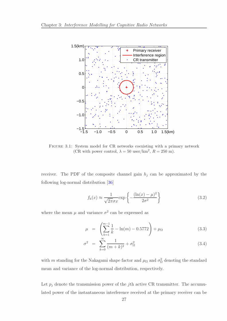
3.1 System model for CR networks coexisting with a primary network (CR with
power control, λ = 50 user/km2, R = 250 m). . . . . . . . . . . . . . . . . 27
3.2 A CR network under contention control or hybrid control scheme coexists
with a primary network (λ = 50 user/km2, dmin = 150m, R = 250 m). . . . 32
3.3 Comparison of interference distributions for power, contention and hybrid
power/contention control schemes (R =100 m, λ =300 user/km2, β =4,
rpwc = 20 m, α = 4, Pmax = 1 W, p = 1 W, dmin = 20 m and rhyb = 30 m) . 38
3.4 Log-normal approximation for interference distribution under (a) power con-
trol (R =100 m, β =4, rpwc = 20 m, α = 4, Pmax = 1 W, µ = 0 and σ = 4
dB) or (b) contention control R =100 m, β =4, dmin = 20 m, p = 1 W,
µ = 0 and σ = 4 dB). . . . . . . . . . . . . . . . . . . . . . . . . . . . . . 41
3.5 Imperfect knowledge of primary receiver location - the primary receiver is
hidden from all CR transmitters distributed in the shaded region. . . . . . . 43
3.6 Log-normal approximation for interference distribution with a hidden pri-
mary receiver under (a) power control (R =200 m, λ =3 user/104m2, β =4,
rpwc = 20 m, α = 4, Pmax = 1 W and rp = 0.5R) or (b) contention control
(R =200 m, λ =3 user/104m2, β =4, dmin = 20 m, p = 1 W and rp = 0.5R). 45
3.7 Impact of hidden primary receiver on interference distribution for CR net-
works under hybrid power/contention control scheme (R =200 m, λ =3
user/104m2, β =4, α = 4, dmin = 20, p = 1 W, rp = 0.5R and rhyb = 30 m). . 47
3.8 Impact of various CR deployment parameters on the aggregated interference
for CR networks with (a) power control (R =100 m, λ =3 user/104m2, β =4,
rpwc = 20 m, α = 4 and Pmax = 1 W) or (b) contention control (R =100 m,
λ =3 user/104m2, β =4, dmin =20 m, and p = 1 W). . . . . . . . . . . . . . 48
xiii
List of Figures
3.9 Impact of shadow fading on the aggregated interference for CR networks
with (a) power control (R =100 m, λ =3 user/104m2, β =4, rpwc = 20
m, α = 4 and Pmax = 1 W) or (b) contention control (R =100 m, λ =3
user/104m2, β =4, dmin =20 m and p = 1 W). . . . . . . . . . . . . . . . . 49
4.1 Block diagram of a CR receiver using interference estimation and can-cellation. . . . . . . . . . . . . . . . . . . . . . . . . . . . . . . . . . . . 61
4.2 Symbol error rate performance of a CR communication link in thepresence of high-power interfering DVB-T signals. . . . . . . . . . . . . 63
4.3 A hybrid IC technique combining beamforming and interference can-cellation/suppression. . . . . . . . . . . . . . . . . . . . . . . . . . . . . 68
4.4 A CR MIMO transmitter-receiver pair coexists with a primary TDDsystem. . . . . . . . . . . . . . . . . . . . . . . . . . . . . . . . . . . . . 71
4.5 System diagram for the proposed precoding schemes. . . . . . . . . . . 73
4.6 CR throughput under different precoding schemes (Mt = Mr = 4,Mbs = 2, K = 2, M1 = M2 = 1, LS1 = LS2 = LT2 = 50, LT1 = 350,σ2H = σ2
ut = 1, Pcr = 1, and rt/d = 0.1). . . . . . . . . . . . . . . . . . . 80
4.7 (a) CR throughput and (b) resulting interference of different precodingschemes (Mt = Mr = 4, Mbs = 2, K = 2, M1 = M2 = 1,, LS = 100,LS1 = LS2 = LT2 = 50, LT1 = 350, σ2
H = 1, Pcr = 1, rt/d = 0.1, andσ2n = 10−4). . . . . . . . . . . . . . . . . . . . . . . . . . . . . . . . . . 81
4.8 System model for multiple CR pairs coexisting with a primary system. 84
4.9 Relationship between CR INR and the average CR-primary interference(Mp = 2, Mc = 4, K = 1, LS1 = LS2 = 50, σ2
H = 1, Pcr = 1 Unit, andσ2n = 10−4). . . . . . . . . . . . . . . . . . . . . . . . . . . . . . . . . . 90
4.10 Performance evaluation of the proposed cross-layer algorithms (r =10m, l = 100m, K = 10, N = 3, Mp = 2, Mc = 4, Ls1 = Ls2 = Ls = 25,Pcr = 1, and σ2
n = 10−4). . . . . . . . . . . . . . . . . . . . . . . . . . . 94
4.11 Convergence of the proposed JICAP algorithm (r = 10m, l = 100m,K = 10, N = 3, Mp = 2, Mc = 4, Ls1 = Ls2 = Ls = 25, Pcr = 1, andσ2n = 10−4). . . . . . . . . . . . . . . . . . . . . . . . . . . . . . . . . . 95
5.1 An example of different signalling schemes and NB solutions of 2-userMIMO interference system. . . . . . . . . . . . . . . . . . . . . . . . . . 110
5.2 An achievable rate region for a 3-user MIMO interference system. . . . 117
5.3 Probability of convex rate region over different values of SIR. . . . . . . 122
5.4 Various bargaining solutions for a MIMO interference system. . . . . . 124
5.5 Existence of the FP-based NB solution for different SNRs and INRs. . . 125
xiv
List of Tables
4.1 Interference mitigation techniques for cognitive radio networks. . . . . . 56
4.2 Comparison of different interference suppression techniques for CR re-ceivers. . . . . . . . . . . . . . . . . . . . . . . . . . . . . . . . . . . . . 60
4.3 Comparison of different interference avoidance techniques applicablefor CR transmitters. . . . . . . . . . . . . . . . . . . . . . . . . . . . . 67
4.4 The JICAP algorithm. . . . . . . . . . . . . . . . . . . . . . . . . . . . 89
5.1 Comparison of various rate region convexification schemes . . . . . . . 114
xv


Abbreviations
1G First Generation
2G Second Generation
3G Third Generation
4G Fourth Generation
AIC Akaike Information Criterion
AWGN Additive White Gaussian Noise
BS Base Station
CPE Customer Premises Equipment
CR Cognitive Radio
CSI Channel State Information
CSMA/CA Carrier Sense Multiple Access with Collision Avoidance
DoF Degrees of Freedom
DSA Dynamic Spectrum Access
DVB-T Digital Video Broadcasting – Terrestrial
EVD Eigenvalue Decomposition
FCC Federal Communications Commission (of United States)
FDM Frequency Division Multiplexing
FP Full Projection
FRESH FREquency SHift Filter
GPS Global Position System
i.i.d. independent and identically distributed
IA Interference Avoidance
IC Interference Cancellation
IM Interference Mitigationxvii

Abbreviations
INR Interference-to-Noise Ratio
IR Interference Region
ISM Industrial, Scientific and Medical
IWF Iterative Water Filling
JFI Jain’s Fairness Index
JICAP Joint Iterative Channel Allocation and Precoding
K-S Kalai-Smorodinsky
MAC Media Access Control
MAI Multi-Access Interference
MCO Multiple Criteria Optimisation
MDL Minimum Description Length
MH Matern Hard-core
MIMO Multiple Input Multiple Output
MISO Multiple Input Single Output
MUD Multi-User Detection
MUSIC MUltiple SIgnal Classification
NB Nash Bargaining
NE Nash Equilibrium
NICAP Non-Iterative Channel Allocation and Precoding
Ofcom Office of Communications (of United Kingdom)
OSA Opportunistic Spectrum Access
OFDM Orthogonal Frequency Division Multiplexing
PDF Probability Density Function
PIC Parallel Interference Cancellation
PP Partial Projection
PSD Positive Spectrum Density
QoS Quality of Service
QPSK Quadrature Phase Shift Keying
RF Radio Frequency
Rx Receiver
SER Symbol Error Rate
xviii

Abbreviations
SIC Successive Interference Cancellation
SINR Signal-to-Interference-plus-Noise Ratio
SIR Signal-to-Interference Ratio
SISO Single Input Single Output
SNR Signal to Noise Ratio
SOI Signal Of Interest
SP Sensing and Projection
STFT Short-Time Fourier Transform
SVD Singular Value Decomposition
TDD Time Division Duplexing
TDM Time Division Multiplexing
TDIR Trivial over Dominant Interference Ratio
TV Television
Tx Transmitter
TFRs Time-Frequency Representations
UMTS Universal Mobile Telecommunications System
UWB Ultra Wide Band
WRAN Wireless Regional Area Network
xix


Symbols
(·)T transpose of a matrix
(·)H Hermitian transpose of a matrix
(·)† pseudoinverse of a matrix
tr[·] trace of a matrix
E[·] statistical expectation operator
rank(·) rank of a matrix
Cx×y the space of x× y complex matrices
∪ union of sets
∩ intersection of sets∑
summation∏
production
Ai channel allocation for ith CR transmitter
A channel allocation for all active CR transmitters
C(x, r) a disk centred at point x with radius r
dnn nearest neighbour distance
dmin minimum distance between two CR transmitters
D radius of a grey space
fp(·) PDF of the transmission power
fλ(λ1, λ2, · · · , λMmin) joint PDF of λ1, λ2, · · · , λMmin
F precoding matrix
Fd precoding matrix for CR during primary downlink
Fi,Aiprecoding matrix for the ith CR transmitter at the
sub-channel Ai
xxi

Symbols
g(rj) pathloss function at distance rj
Gk channel matrix from the CR transmitter to the kth
primary user
GU,i,Ai, GD,j,Aj
interference channels from the primary user to the
ith CR transmitter during uplink and from the
primary BS to the jth CR receiver during downlink
hj channel gain from jth CR Tx to the primary Rx
H MIMO channel matrix
Hur primary-CR Rx interference channel during uplink
Hut primary-CR Tx interference channel during uplink
Hdr primary-CR Rx interference channel during downlink
Hdt primary-CR Tx interference channel during downlink
H⊥ effective CR channel matrix after projection
Hi,j channel matrix from the Tx i to the Rx j
Hi,j,Aichannel matrix from the ith CR Tx to the jth
CR Rx over sub-channel Ai
i√−1
i, j index for CR users
Ii(Q) mutual information for user i with transmit
covariance matrices Q
INEi mutual information for user i at NE
Inti average interference caused by the ith CR
transmitter to the primary user
Intl CR-primary interference at low CR INRs
Inth CR-primary interference at high CR INRs
IntFPh
CR-primary interference due to FP precoding at high
CR INRs
IntPPh
CR-primary interference due to PP precoding at high
CR INRs
I identity matrix
J Jain’s fairness index
xxii

Symbols
kn nth cumulant of the aggregate interference
K total number of CR users
Kp an estimate of active primary antenna numbers
l radius of a disk centred at the primary receiver
L radius of black space
LS length of sensing for SP precoding
LS1 length of sensing during primary uplink
LS2 length of sensing during primary downlink
LT length of transmission for SP precoding
LT1 length of downlink transmission
LT2 length of uplink transmission
m Nakagami shape factor
Mt, Mr, Mbs and Mk number of antennas for CR transmitter, CR receiver,
primary base BS and the kth primary user
Mmin minimum number of antennas
Mmax maximum number of antennas
n general index
n noise vector in MIMO channels
N number of subchannels for primary networks
N ri number of antennas at receiver i
N ti number of antennas at transmitter i
p transmission power under contention control
Pcr maximum average CR transmission power
pj transmission power of the jth CR transmitter
Pp transmission power of each primary user antenna
ppwc transmission power under power control
phyb transmission power under hybrid control
Pmax the maximum CR transmission power
qmh retaining probability of MH thinning
Q a set of transmit covariance matrices
Qi transmit covariance matrix for user i
xxiii

Symbols
Qu, Qd transmit covariance matrix for primary user
during uplink and downlink
rccj nearest neighbouring CR-CR distance for jth CR
rcp distance between CR Tx and primary Rx
rhyb power control range for hybrid control scheme
rj distance between the jth CR Tx and primary Rx
rp distance between the primary Tx-Rx pair
rpwc power control range for the power control scheme
rt/d maximum ratio of the resulting to nullified interference
ri,j,Ai(t) the tth received signal at CR Rx j
during the time slot of CR pair i at subchannel Ai
rut(t) the tth received symbol at the CR transmitter
rut,i,Ai(t) the tth received symbol at the ith CR
transmitter at subchannel Ai
R radius of IR
Ri rate for user i
R−i INR covariance matrix for user i
Ri,j,Aicovariance matrix of ri,j,Ai
Rut covariance matrix of rut
Rut estimated Rut
Rut,i,Aicovariance matrix of rut,i,Ai
S bargaining set
Sn set of cochannel CR users
s the transmit information vector
t time index
U, Ud, Un, UG, U⊥ unitary matrices from SVD
V, Vd, Vn, VG, V⊥ unitary matrices from SVD
xu transmitted signal vector of all the K primary users
xd transmitted signal vector of the primary BS
x(n)i decoded signal vector at the receivers i
y received signal vector
xxiv

Symbols
Y aggregated CR-primary interference
z interference signal vector
Z interference covariance matrix
α power control exponent
β pathloss exponent
φY characteristic function of the aggregate interference
ηji normalised INR from transmitter j to receiver i
λ density of a stationary Poisson point process
λi the ith eigenvalue of a matrix
µ mean value
µΩ standard mean of a log-normal distribution
ρi normalised SNR for user i
σ2 variance value
σ2Ω standard variance of a log-normal distribution
τ fraction of convex combination
θ the angle between the line joining primary Tx and
CR Tx and the line joining primary Tx-Rx pair
ω variable in frequency domain
Φ stationary Poisson point process
Φth thinned stationary Poisson point process
Φmh Matern hard-core point process
Γk interference temperature limit for primary user k
Λ1/2, Λ1/2d , Λ
1/2n , Λ
1/2G , Λ
1/2⊥ diagonal eigenvalue vectors from SVD
xxv


Chapter 1
Introduction
1.1 Problem Statement
Wireless communication is one of the few technologies that have significantly changed
lives of human beings. In 1901, Marconi convincingly demonstrated the practicality
of wireless communication by sending the first radio signal across the Atlantic, and a
new era was born ever since then. After evolving over a century, wireless communi-
cation can find its applications in various aspects of our lives nowadays, ranging from
highly commercialised cellular and satellite communication systems to privately used
amateur radio, from daily used WiFi networks to rarely seen deep space communica-
tion systems, from infrastructure-based radio and television broadcast systems to ad
hoc-oriented wireless microphones and Bluetooth devices. New wireless applications
are still keeping emerging as the demand for them never stops.
Radio spectrum, the indispensable media underpinning a wireless communication sys-
tem, is conventionally assigned to each wireless application for exclusive use by regu-
latory bodies like Federal Communications Commission (FCC) in the USA and Office
of Communications (Ofcom) in the UK. It is becoming increasingly scarce as more
and more devices go wireless. Meanwhile, studies indicate that there is a vast amount
of spectrum not fully utilised in the domain of time, frequency and space [1]. Mea-
surement campaigns have shown that up to 85% of the spectrum is wasted temporally
1

Chapter 1: Introduction
in some bands below 3 GHz [2, 3]. The imbalance between the plausible spectrum
scarcity and eventual spectrum underutilisation has inspired a revolutionary paradigm
shift on spectrum access by allowing the spectrum to be shared and reused in a dy-
namic manner, which is known as dynamic spectrum access (DSA) [4]. Cognitive
radio (CR) is a prominent candidate technology enabling the DSA. It is capable of
sensing its surrounding environment and adapting its operational parameters dynam-
ically and autonomously to coexist with the incumbent systems (primary systems) in
a nonintrusive manner [1]. It is envisioned as a promising solution to greatly improve
the spectrum utilisation by reusing the underutilised spectrum owned by primary
systems.
Interference is one of the key factors affecting the wireless network performance and
has been a long-lasting problem coupling wireless communication systems. It is by no
means an exaggeration to say that wireless communication is nothing but combating
interference and impairment of wireless channels. In the context of CR networks,
the interference issues are extremely important. Its paramount significance lies on
two aspects. On one hand, CR holds the fundamental premise of not causing any
detrimental interference to the primary system. On the other, CR performance may by
limited by interference coming from either the primary or other CR nodes. Therefore,
the interference related issues in CR networks deserve careful and comprehensive
study, which is the main focus of this thesis.
1.2 Motivation
With the introduction of CR networks, two novel types of interference originating from
CR networks are introduced. They are the interference from CR to primary networks
(CR-primary interference) and the interference among spectrum-sharing CR nodes
(CR-CR interference). The former is caused by spectrum sharing between CR and
primary networks. While, the latter is due to spectrum sharing among CR nodes.
Both types of interference should be well managed by CR networks in order not to
2

Chapter 1: Introduction
jeopardise the operation of the primary network and to improve the performance of
CR systems. This motivates the research conducted in this thesis.
For the CR-primary interference, it is desirable to investigate how CR networks poten-
tially affect the primary system. This requires interference modelling for CR networks
to examine the impact of CR operation on the resulting CR-primary interference. It
consequently gives clue for the deployment of CR networks aiming at minimising the
CR-primary interference. Moreover, interference mitigation techniques applicable to
CR networks are worth studying to further reduce the CR-primary interference. Phys-
ical layer signal processing has been widely used in interference mitigation. We can
also perform the interference mitigation more effectively from a cross-layer perspec-
tive.
When multiple CR links share the spectrum, the CR-CR interference is inevitable.
This naturally raises the problem of how to coordinate the mutually interfering CR
nodes. The interference channels can be analysed by characterising the rate region
of CR interference systems. Various signalling and interference mitigation techniques
applicable to spectrum-sharing CR nodes need to be investigated by analysing their
resulting rate regions.
1.3 Contributions
The key contributions of the thesis are summarised as follows:
• Modelling the CR-primary interference:
Wemodel the aggregate CR-primary interference by deriving its probability den-
sity function (PDF) for CR networks under different interference management
mechanisms, including power control, contention control and hybrid power/con-
tention control schemes. The impact of key CR operational parameters on the
resulting CR-primary interference is investigated. The effect of hidden primary
receiver on the CR-primary interference is examined as well.
3

Chapter 1: Introduction
• Mitigating the CR-primary interference:
We first carry out a comprehensive review on a variety of interference mitigation
techniques applicable to CR networks, including interference cancellation at CR
receivers and interference avoidance at CR transmitters. Then, we focus on
mitigating the CR-primary interference for CR multiple-input multiple-output
(MIMO) systems. Two precoding-based interference avoidance schemes are pro-
posed for CR MIMO systems to avoid interfering with the primary network and
to boost the throughput of the CR system. To better mitigate the CR-primary
interference, we perform the interference mitigation in a cross-layer manner by
jointly considering precoding in the physical layer and channel allocation in the
media access control (MAC) layer. Two distributed algorithms are proposed for
the cross-layer interference mitigation.
• Analysing the CR-CR interference channels:
We confine our attention to analysing multi-user CR MIMO interference sys-
tems. The Pareto rate region for MIMO interference systems are characterised
by finding a sufficient condition for the convexity of the rate region. Then, var-
ious rate region convexification approaches including orthogonal signalling and
interference mitigation techniques are examined and their resulting rate regions
are analysed for the MIMO interference system. An achievable rate region is
also given for multi-user MIMO interference systems. Finally, we apply Nash
bargaining (NB) to coordinate the interfering CR users. The characteristics of
the NB over MIMO interference systems such as the existence, uniqueness and
optimality are studied.
The work presented in this thesis has led to the following publications:
Journals
1. Z. Chen, C.-X. Wang, X. Hong, J. Thompson, S. A. Vorobyov, F. Zhao, H.
Xiao, and X. Ge, “Interference mitigation for cognitive radio MIMO systems
4

Chapter 1: Introduction
based on practical precoding,” IEEE Trans. Veh. Technol., submitted for pub-
lication, 2011.
2. Z. Chen, S. A. Vorobyov, C.-X. Wang, and J. Thompson, “Pareto region charac-
terisation for rate control in MIMO interference systems and Nash bargaining,”
IEEE Trans. Autom. Control, submitted for publication, 2011.
3. Z. Chen, C.-X. Wang, X. Hong, J. Thompson, S. A. Vorobyov, X. Ge, H. Xiao,
and F. Zhao, “Aggregate interference modeling in cognitive radio networks with
power and contention control,” IEEE Trans. Commun., accepted for publica-
tion, Mar. 2011.
4. X. Hong, Z. Chen, C.-X. Wang, and S. A. Vorobyov, “Cognitive radio networks:
interference cancellation and management techniques,” IEEE Veh. Technol.
Mag., vol. 4, no. 4, pp. 76–84, Dec. 2009.
Conferences
1. Z. Chen, C.-X. Wang, X. Hong, J. S. Thompson, S. A. Vorobyov, and D. Yuan,
“Cross-layer interference mitigation for MIMO cognitive radio systems,” in Proc.
IEEE ICC’11, Kyoto, Japan, June 2011, accepted for publication.
2. Z. Chen, C.-X. Wang, X. Hong, J. Thompson, S. A. Vorobyov and X. Ge,
“Interference modeling for cognitive radio networks with power or contention
control,” in Proc. IEEE WCNC’10, Sydney, Australia, Apr. 2010.
3. Z. Chen, S. A. Vorobyov, C.-X. Wang, and J. S. Thompson, “Nash bargaining
over MIMO interference systems,” in Proc. IEEE ICC’09, Dresden, Germany,
June 2009.
1.4 Thesis Organisation
The remainder of this thesis is organised as follows:
5
Chapter 1: Introduction
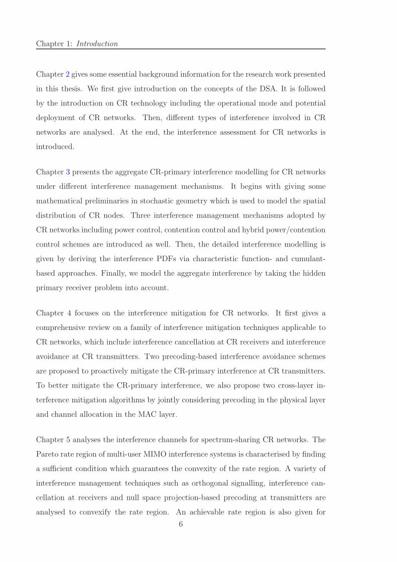
Chapter 2 gives some essential background information for the research work presented
in this thesis. We first give introduction on the concepts of the DSA. It is followed
by the introduction on CR technology including the operational mode and potential
deployment of CR networks. Then, different types of interference involved in CR
networks are analysed. At the end, the interference assessment for CR networks is
introduced.
Chapter 3 presents the aggregate CR-primary interference modelling for CR networks
under different interference management mechanisms. It begins with giving some
mathematical preliminaries in stochastic geometry which is used to model the spatial
distribution of CR nodes. Three interference management mechanisms adopted by
CR networks including power control, contention control and hybrid power/contention
control schemes are introduced as well. Then, the detailed interference modelling is
given by deriving the interference PDFs via characteristic function- and cumulant-
based approaches. Finally, we model the aggregate interference by taking the hidden
primary receiver problem into account.
Chapter 4 focuses on the interference mitigation for CR networks. It first gives a
comprehensive review on a family of interference mitigation techniques applicable to
CR networks, which include interference cancellation at CR receivers and interference
avoidance at CR transmitters. Two precoding-based interference avoidance schemes
are proposed to proactively mitigate the CR-primary interference at CR transmitters.
To better mitigate the CR-primary interference, we also propose two cross-layer in-
terference mitigation algorithms by jointly considering precoding in the physical layer
and channel allocation in the MAC layer.
Chapter 5 analyses the interference channels for spectrum-sharing CR networks. The
Pareto rate region of multi-user MIMO interference systems is characterised by finding
a sufficient condition which guarantees the convexity of the rate region. A variety of
interference management techniques such as orthogonal signalling, interference can-
cellation at receivers and null space projection-based precoding at transmitters are
analysed to convexify the rate region. An achievable rate region is also given for
6

Chapter 1: Introduction
multi-user MIMO interference systems. Finally, NB is applied to coordinate the op-
eration of interfering CR users. The characteristics of different NB solutions over
MIMO interference systems such as uniqueness, existence and optimality are studied.
Chapter 6 concludes the thesis and suggests some future research topics.
7


Chapter 2
Background
2.1 Status Quo of Radio Spectrum
Radio spectrum refers to the part of electromagnetic spectrum corresponding to radio
frequencies - that is, frequencies lower than around 300 GHz [5]. It is the indispensable
media carrying any wireless communication. By nature, radio spectrum is a precious
and limited natural resource. For wireless systems operating in very low frequencies,
the effective antenna size has to be very large, which is not feasible for portable wire-
less devices. As for spectrum with high frequencies, the wireless channel becomes
too hostile for the propagation of electromagnetic waves. Therefore, only a limited
range of spectrum is usable for wireless communications. This range of radio spec-
trum is usually divided into non-overlapping bands and assigned to different wireless
applications for exclusive use to avoid mutual interference. The spectrum allocation
is typically government regulated by regulatory agencies like FCC in the USA and
Ofcom in the UK. Some bands are allocated to certain applications free of charge,
e.g., the industrial, scientific, and medical (ISM) band for cordless telephones or wire-
less computer networks. Other bands are licensed or sold to private communication
systems like cellular telephone operators and satellite communication companies.
The spectrum allocation in the USA is shown in Figure 2.1. Even a casual observer
can easily tell from the figure that the radio spectrum has been fully “booked” due to
9

Chapter 2: Background
Figure 2.1: U.S. frequency allocations chart [6].
its “overcrowded” looking. It seems that the spectrum is too scarce to accommodate
new wireless applications. The demand for bandwidth (radio spectrum), however,
never stops by newly emerging wireless services. One representative example is cellular
mobile communication, mobile communication systems have evolved from the voice
oriented first generation (1G) and second generation (2G) to the multimedia-rich
third (3G) and fourth generations (4G) over the last three decades. The technology
evolution in mobile communication is driven by exponential increase in throughput
demand and needs to acquire additional bands to operate on. The conflicts between
spectrum availability and spectrum demand has incurred widely spread anxiety of
spectrum scarcity. This can be reflected by the record-breaking auction of British 3G
spectrum in early 2000. The UK 3G - Universal Mobile Telecommunications System
(UMTS) spectrum licenses were sold for the extraordinary sums of £22 billions to five
operators with only a 20-year tenure of use.
Despite the widely perceived spectrum scarcity, spectrum measurements unveil an
astonishing fact on spectrum utilisation. Studies undertaken by the FCC [2] and
10

Chapter 2: Background
Figure 2.2: Spectrum occupancy measurements in a rural area (top), nearHeathrow airport (middle) and in central London (bottom) [3].
the Ofcom [3] have revealed that the spectrum utilisation shows huge temporal and
spatial variations ranging from 15 to 85% for spectrum below 3 GHz. An example of
spectrum usage measurement in England is shown in Figure 2.2. These measurement
campaigns indicate that a vast amount of spectrum bands are not fully used all the
time or everywhere. In another word, the radio spectrum is eventually underutilised.
It has been commonly accepted that the fixed spectrum allocation and the exclusive
use of spectrum make the spectrum underutilised and appear scarce. There is potential
to make considerably better use of spectrum if the spectrum is used in a more dynamic
and flexible manner.
2.2 Dynamic Spectrum Access
The imbalance between plausible spectrum scarcity and eventual spectrum under-
utilisation has inspired enormous research on DSA. In contrast to the current fixed
spectrum access policy where spectrum is allocated for exclusive use, DSA intro-
duces a revolutionary paradigm shift on spectrum management by introducing much
more flexibility into spectrum access. It allows the spectrum to be shared and reused
11

Chapter 2: Background
Figure 2.3: A taxonomy of dynamic spectrum access [4].
among different wireless applications on a negotiable or opportunistic basis. There-
fore, it has the potential to greatly improve the spectrum utilisation. As illustrated in
Figure 2.3, DSA can be broadly divided into three categories according its operation
model [4].
• Dynamic exclusive use model
It shares the similar philosophy with current fixed spectrum access in that the
spectrum is rigidly for exclusive use once allocated, but it allows more flexibility
in spectrum allocation. This can be achieved via either spectrum property rights
or dynamic spectrum allocation. The former allows licensed spectrum holders
lease or trade their spectrum freely with other wireless operators. For example,
TV broadcasters may temporarily lease parts of TV bands to mobile operators to
provide cellular network coverage for special festivals or events. While, the latter
allocates the spectrum in a more dynamic manner in terms of time and location
according to the traffic characteristics of different services. For instance, the
spectrum allocation can be performed more frequently, e.g., hourly, for wireless
applications with rapidly changing traffic load.
• Open sharing model
In this model, peer users sharing the spectrum openly with equal access rights
and priorities. An example of wireless network adopting this model is WiFi,
which shares the ISM band freely and fairly with many other wireless systems
like Bluetooth devices, cordless telephones, etc.
12

Chapter 2: Background
• Hierarchical access model
This model differs from open sharing model in that spectrum users working
in hierarchical access model have different priorities and are distinguished as
primary and secondary users. Primary users who own the spectrum have the
absolute privilege to use the spectrum. While, secondary users do not have the
license to use the spectrum. They can reuse it only in a nonintrusive manner.
To use an analogy, primary users are “hosts”, while secondary users are like
“guests”. This model can be further divided into two subcategories: spectrum
underlay and spectrum overlay. In spectrum underlay approach, the transmis-
sion power spectrum density (PSD) of secondary users is strictly constrained
by a predefined spectral mask so that the PSD of secondary transmission is
below that of the noise for primary users. Primary users can simply treat the
secondary interference as background noise. Ultra wide band (UWB) systems is
a representative example of this approach. They maintain a very low PSD for
secondary transmission by spreading the secondary signals into a very wide band
of spectrum [7]. Whereas, for spectrum overlay, no predefined PSD constraint
is imposed on secondary users. Instead, secondary users can identify and ex-
ploit the spectrum opportunity without detrimentally interfering with primary
users. This is also known as opportunistic spectrum access (OSA). The newly
emerging CR serves as an enabling technology for OSA.
2.3 Cognitive Radio Technology
CR, first coined by Mitola in 1998 [8, 9], is a “smart” radio system aware of its
surrounding operational environment by sensing and reasoning, and capable of dy-
namically and autonomously adjusting its radio operating parameters to coexist with
the primary users in a nonintrusive manner [1, 10, 11]. CR is envisioned as a promising
technology to improve the spectrum utilisation by sharing the underutilised spectrum
with the legacy users in a hierarchical manner without causing detrimental interfer-
ence to the primary network.
13

Chapter 2: Background
To facilitate the nonintrusive coexistence with primary users, a CR is supposed to
have a set of cognitive capabilities as illustrated in Figure 2.4 [10]. The following
three main capabilities need to be incorporated throughout the whole cognitive cycle.
• Spectrum sensing
Intuitively, how to find out the available spectrum holes from a spectrum pool,
is the first step for a CR. In this step, the radio environment is constantly mon-
itored, and spectrum holes are detected by a CR. Spectrum holes, also known
as frequency voids or white spaces, refer to frequency segments that are orig-
inally licensed to the primary network, but unused or partly occupied by the
primary system temporally or in some geographical locations. Spectrum sensing
can be performed by using energy detection [12] or cyclostationary feature de-
tection [13] across the spectrum pool. Cooperative spectrum sensing has gained
much recognition as a more appealing sensing technique in terms of detection
accuracy [14].
• Spectrum analysis
Figure 2.4: Cognitive cycle of CR systems [10].
14

Chapter 2: Background
The spectrum holes information is analysed in this phase. The characteristics
of spectrum holes, such as the interference level they suffers and the channel
capacity they can offer, are estimated and forwarded to the next also the final
stage.
• Spectrum decision
A CR network synthesises all the information from spectrum sensing, spectrum
analysis and CR user demand to determine which spectrum band to choose and
how the transmission should be carried out.
According to the way that CR systems reuse the spectrum, a CR network can operate
on a non-interfering or interference-tolerant basis.
2.3.1 Non-interfering Cognitive Radio
For non-interfering (or interference-free) CR [15, 16], as the name suggests, theoreti-
cally it does not cause any interference to the primary system by only reusing spectrum
holes that are not occupied by the primary users. That is, only white spaces of the
primary system are exploited by the CR network. Obviously, CR working in a non-
interfering manner is favourable to the primary network, since the quality-of-service
(QoS) of primary network is not compromised at all. Moreover, the primary system
does not need to be aware of the existence of the CR users, i.e., no modification is
required in primary systems to accommodate CR applications, because CR systems
always “avoid” the primary transmission “automatically”. Therefore, non-interfering
CR is chosen by the IEEE 802.22 working group as the enabling technique for the
first standardised CR network - wireless regional area network (WRAN) [17].
WRAN aims at providing wireless broadband access service in lightly populated rural
areas by using non-interfering CR technique to share the geographically unused TV
bands licensed to television broadcasters [18]. The initial 802.22 standard specifies
that a WRAN works in a point to multipoint manner. It consists of a base station
(BS) and customer premises equipments (CPEs). Each CPE is attached to a BS. The
15

Chapter 2: Background
BS is a central controller managing the access of CPEs that attach to it. A WRAN
can operate in two approaches. One approach is based on spectrum sensing. Each
CPE performs independent sensing in the TV bands and reports the sensing result to
the BS regularly. The BS gathers and analyses the sensing information from all the
associated CPEs and instructs each CPE which band it should operate on. The other
approach is geo-location based. All the BS and CPEs are capable of finding their
own location using some location identification techniques like the Global Positioning
System (GPS). With their location information, the BS determines the channels that
the associated CPEs can use by regularly looking up an incumbent database. The
incumbent database keeps the live information of licensed TV operation in any given
geographical location and it is usually maintained by spectrum regulatory bodies.
2.3.2 Interference-Tolerant Cognitive Radio
In contrast to non-interfering CR, interference-tolerant CR [19–21] can share the whole
spectrum with the primary system (including the bands that are being used by primary
users), but the interference experienced at the primary receiver from CR networks
must be maintained below a specific level without causing any outage on primary
operation. In another word, the CR system can reuse the whole spectrum so long as
the primary network can “tolerate” it. To implement an interference-tolerant CR, the
primary receiver has to provide CR systems the information of how much interfer-
ence it can tolerate across the spectrum, which is known as interference temperature
limit. Thus, a real-time feedback mechanism from the primary to the CR networks is
essential to inform the CR network of the interference temperature limit. In order to
facilitate this functionality, some modification on the primary system is inevitable.
It is easy to understand that non-interfering CR is a transmitter-centric approach since
it indirectly controls the potential CR-primary interference by regulating CR trans-
mitters to only exploit spectrum holes. While, interference-tolerant CR is receiver-
centric due to the fact that the primary receiver directly controls the CR-primary
interference by giving CR networks the interference temperature limit. Moreover,
interference-tolerant CR leads to higher spectrum utilisation than non-interfering CR,
16
Chapter 2: Background
since the former has more available spectrum than the latter. However, interference-
tolerant CR needs the intervention of the primary network to acquire the interfer-
ence temperature limit. The requirement for the primary network intervention makes
interference-tolerant CR undesirable or even infeasible sometimes. Therefore, peo-
ple commonly regard non-interfering CR as the first generation CR networks and
interference-tolerant CR as a long-term evolution goal.
2.4 Interference in Cognitive Radio Networks
Interference involved in CR networks can be classified into two types: intra-network
interference and inter-network interference. Intra-network interference, also known as
self-interference, refers to the interference caused within one network (either a primary
or CR network). Typical examples of intra-network interference include inter-symbol
interference in frequency selective channels and multi-access interference (MAI) in
multi-user networks. Intra-network interference exists to some extent in every wireless
communication system and there is a wealth of techniques established to mitigate
them effectively. On the other hand, inter-network interference refers to the mutual
interference between the primary and CR networks. The problem of inter-network
interference management is two-fold. First, CR transmitters need to carefully control
their emissions to guarantee that the QoS of the primary network is not harmfully
degraded by the CR-primary interference. Second, CR receivers should be able to
effectively combat the primary-CR interference and provide useful QoS to the CR
application. We first give an introduction on the characteristics of the inter-network
interference.
17

Chapter 2: Background
2.4.1 CR-Primary Interference
To assess the CR-primary interference in interference-tolerant CR systems, a new met-
ric - interference temperature has been proposed in [10]. Unlike traditional transmitter-
centric approaches that seek to regulate interference indirectly by controlling the emis-
sion power, time, or locations of interfering transmitters, the interference temperature
model takes a receiver-centric approach and aims to directly manage interference at
primary receivers through interference temperature limits. The interference tempera-
ture limit characterises the “worst case” interfering scenario in a particular frequency
band and at a particular geographic location for primary receivers [10, 22]. In other
words, it represents the maximum amount of interference that the primary receiver
can tolerate.
The interference temperature model serves as a useful tool to characterise the CR-
primary interference. An ideal interference temperature model should account for the
cumulative radio frequency (RF) energy from multiple CR transmissions and sets a
maximum cap on their aggregate level. CR users are then allowed to use a frequency
band as long as their transmissions do not violate the interference temperature limits.
Implementation of such an ideal interference temperature model usually requires real-
time interactions between CR transmitters and primary receivers and is therefore
widely regarded as impractical. To this end, several modified interference models
[23, 24] have been proposed as more practical models for the CR-primary interference
received at primary receivers.
In [23], the interference was defined as the expected fraction of primary users with
services disrupted by nearby CR transmitters. Factors such as CR signal modulation,
antenna gains, and power control were considered in this model. However, this model
only accounted for the case where the primary services were disrupted by a single CR
user and it did not consider the aggregate effect of multiple CR transmissions. In [24],
the aggregate effect was taken into account and complex stochastic models were built
to characterise the exact PDF of the accumulated interference power. Moreover, the
interference avoidance ability of CR transmitters was considered by introducing the
concept of an exclusion region. As illustrated in Figure 2.5, an exclusion region is
18

Chapter 2: Background
Figure 2.5: Coexistence of a primary network and randomly distributed CR net-works with illustrations of the exclusion region, black space (service region), grey
space (interfering region), and white space.
defined as a disk centred at a primary receiver with a radius R. Any CR transmitter
within the exclusion region is regarded as a harmful interferer and is therefore for-
bidden to transmit. When the locations of CR transmitters follow a Poisson point
process with a density λ, the PDF of the aggregate interference can be computed as
a function of R. As shown in Figure 2.6, it is found that a slight increase of R can
effectively reduce both the mean and variance of the received interference power. The
CR-primary interference modelling is further extended in [25] by taking into account
interference management schemes for CR networks including power and contention
control. The detailed modelling will be presented in Chapter 3. To combat the
CR-primary interference, several interference mitigation schemes will be proposed in
Chapter 4.
19

Chapter 2: Background
0 5 10 15 200
0.1
0.2
0.3
0.4
0.5
0.6
0.7
0.8
0.9
1
Normalized aggregate interference power
Agg
rega
te in
terf
eren
ce p
ower
PD
F
R = 0 mR = 0.8 mR = 1 mR = 1.3 m
Figure 2.6: PDFs of the aggregate interference power (normalised to the transmitpower of the interferers) with different values of the exclusion region radius R (CR
transmitter density λ = 1) [24].
2.4.2 Primary-CR Interference
The interference from primary to CR networks can be directly measured by CR re-
ceivers with passive sensing techniques. Based on the PSD of the interfering primary
signals, we can broadly classify the spectra into three categories: (i) Black spaces are
spectra occupied by high-power primary signals, which have high probability to be
decoded by CR receivers; (ii) Grey spaces refer to spectra with low to medium power
primary signals, which are too weak to be decoded satisfactorily but are still signif-
icant sources of interference to the CR network; (iii) White spaces refer to spectra
where primary signals have negligible power and can be simply treated as background
noise.
Characterising the distributions of white/grey/black spaces across frequency, time,
and space domains are of great importance for assessing the interference faced by CR
20
Chapter 2: Background
receivers. To date, such a characterisation has mainly been conducted empirically by
a number of measurement campaigns [1], which show that the radio spectrum consists
of a high percentage of white space. A theoretical model was recently proposed in [26]
to characterise the spatial distributions of white/grey/black spaces in the presence of a
random primary network with homogeneous nodes. There, it was assumed that every
active primary transmitter uniquely defines a black space area and a grey space area.
As illustrated in Figure 2.5, the black space area, often considered as the service
region of the primary transmitter, is given by a circular disk with radius L centred at
the primary transmitter. The grey space area, on the other hand, is an outer ring with
radius D surrounding the service region and is regarded as the interfering region to
CR systems. Under an intra-network interference constraint that prohibits two active
primary transmitters to lie closer than a minimum distance of L +D, in [26] it was
found that white/grey spaces are naturally abundant but geographically fragmented.
For example, when D = 2L, the spectra will be detected as white spaces on more
than 56% of the plane and as grey spaces on more than 34% of the plane [26].
Intuitively, white spaces are the most desirable resources for CR networks to exploit,
while grey spaces can also be reused to further improve the spectrum utilisation. There
is a widespread perception that black spaces are not exploitable by CR networks due
to the presence of strong interfering primary signals. In Chapter 4, we will review
different interference cancellation techniques applicable to a CR receiver operating in
white, grey, or even black spaces.
2.4.3 CR-CR Interference
The intra-network interference can be further classified into two types: interference
within primary networks and CR-CR interference. The interference within primary
networks has nothing to do with CR networks. Therefore, it is out of the scope of
this thesis. As for CR-CR interference, it has no fundamental difference from intra-
network interference within other networks, except that CR users hold the premise of
not detrimentally interfering with the primary system in the first place. CR-CR inter-
ference is a main source limiting the performance of spectrum-sharing CR networks.
21

Chapter 2: Background
In Chapter 5, we will evaluate the performance of CR-CR interference channels and
investigate how to coordinate multiple CR users using different interference manage-
ment schemes.
22

Chapter 3
Interference Modelling for
Cognitive Radio Networks
3.1 Introduction
Due to the spectrum sharing nature, a CR network can utilise the spectrum more
efficiently when coexisting with a primary system on the interference-tolerant ba-
sis. In this case, the CR-primary interference should be carefully managed and well
maintained below a certain level by the CR network to protect the primary system.
Therefore, it is desirable to model the CR-primary interference to reveal how the ser-
vice of the primary network is deteriorated and how CR networks may be deployed.
This chapter aims to model and analyse the characteristics of the CR-primary inter-
ference when multiple CR nodes coexist with the primary system. The relationship
between CR operating parameters and the resulting CR-primary interference is inves-
tigated. Moreover, some insights are given on the deployment of the CR network to
better protect the primary system.
In the literature, the existing research on interference modelling for CR networks
mainly falls into three categories: spatial, frequency-domain and accumulated in-
terference modelling. For spatial interference modelling, as the name suggests, the
interference is examined according to the geographical location. The fraction of white
23

Chapter 3: Interference Modelling for Cognitive Radio Networks
spaces available for CR networks was investigated in [27] and [26]. In [28], the region
of interference for CR receivers and region of communication for CR transmitters were
studied for the case where a CR network coexists with a cellular network. The inter-
ference from CR devices to wireless microphones operating in TV bands was analysed
in [29], where the loss of reliable communication area of a wireless microphone due to
the existence of CR devices was examined.
CR interference can also be modelled in the frequency domain. For example, an
experimental study on the interference due to out-of-band emission of a WRAN was
reported in [30]. On one hand, the interference received at the neighbouring bands of
the WRAN operation band was evaluated via measurements. On the other hand, the
maximum allowable radiated power for WRAN end-user devices in each neighbouring
band of a digital television (TV) receiver was determined.
Finally, as for accumulated interference modelling, the aggregate interference in a
given location and at a given frequency band is modelled. Usually, the PDF of the
aggregate interference and the outage probability of a primary receiver due to the
interference are two commonly-used statistics for the aggregate interference modelling.
In [31], the aggregate interference power from a sea of CR transmitters surrounding
a primary receiver was derived. The performance of a primary system was evaluated
in [32] in terms of outage probability caused by the interference from CR networks.
The outage probability was derived for both underlay and overlay spectrum sharing
cases. In [33] the aggregate interference from multiple CR transmitters following a
Poisson point process was approximated by a Gamma distribution and the probability
of interference at a primary receiver was also given. It is worth noting that only
pathloss was assumed for the interfering channel in [31–33]. Their work was extended
by taking both shadowing and fading into account in [24] and [34]. Moreover, the PDF
for accumulated interference and outage probability due to the aggregate interference
from CR nodes were also derived in [24] and [34], respectively.
However, in all the previous works [24, 26–34], the CR transmitters were assumed
to transmit at a fixed power level, i.e., no power control for CR transmitters was
considered. Moreover, the CR nodes were all assumed to communicate with each other
24
Chapter 3: Interference Modelling for Cognitive Radio Networks
simultaneously. Thus, no contention control scheme was employed at the cognitive
MAC layer. In this chapter, we extend the aggregate interference modelling employing
various interference management mechanisms, e.g., power/contention control schemes.
The contribution of this chapter can be summarised as follows.
• A realistic power control scheme is proposed, and a hybrid power/contention
control scheme is introduced.
• The PDFs of interference perceived at a primary receiver from a CR network
are derived numerically for the cases of power or contention control. The inter-
ference distribution of the hybrid control scheme is also analysed and compared
with that of the pure power control and pure contention control schemes by
simulations.
• To reduce the complexity of the numerical interference PDF’s computation,
cumulant-based approximations are applied to fitting the interference distribu-
tions for the first two interference management schemes.
• The impact of the hidden primary receiver problem on the aggregate interference
is investigated for all the three interference management schemes.
The interference modelling presented in this chapter considers several basic interfer-
ence management schemes, which forms a fundamental basis for the development of
other advanced interference models for CR networks. Secondly, it gives insights into
CR deployment by figuring out how to optimise CR operation parameters. Finally,
the interference modelling lays a foundation for performance evaluation of primary
networks, e.g., outage capacity of primary systems can be derived based on the inter-
ference PDFs.
The remainder of this chapter is organised as follows. The system model is elabo-
rated in Section 3.2. Some preliminaries in stochastic geometry which underpins the
interference modelling are introduced in this section as well. The detailed interference
modelling is presented in Section 3.3 when perfect knowledge of the primary system
is known to the CR network. In Section 3.4, the hidden primary receiver problem is
25

Chapter 3: Interference Modelling for Cognitive Radio Networks
taken into account for the interference modelling, i.e., scenarios with imperfect pri-
mary system knowledge. The impact of several key parameters on the interference
is analysed via numerical studies in Section 3.5. Finally, Section 3.6 concludes this
chapter.
3.2 System Model
The system model is illustrated in Figure 3.1. It consists of a CR network coexisting
with a primary transmitter-receiver pair. The interference region (IR) is adopted by
the primary network to protect itself against interference from the CR network. No
CR transmission is allowed within the IR. There exist two main types of techniques
to identify the IR for a primary network: geo-location technique and spectrum sens-
ing [35]. For geo-location-based CR networks, the GPS can be incorporated within
the CR network. It enables CR transmitters to determine whether they are located far
enough outside the protected service contour of the primary system. The geo-location
technology usually leads to a circular IR around the primary system. As for spectrum-
sensing-based CR, the IR is usually not circular but more irregular than that of the
geo-location-based CR due to fading and/or imperfect sensing. In this chapter, we
focus on the former type and thus, a circular IR with a radius R is considered.
The underlying interference channels from CR transmitters to the primary receiver
experience pathloss, shadowing and fading. The pathloss function g(rj) is
g(rj) = r−βj (3.1)
where rj is the distance between the jth (j = 1, 2, · · · ) active CR transmitter and the
primary receiver and β is the pathloss exponent. The composite model for shadowing
and fading can be expressed as the product of the long term shadowing and the short
term multipath fading. In this chapter, log-normal shadowing and Nakagami fading
are considered. Let hj denote the channel gain for the composite shadowing and
fading of the interference channel from the jth active CR transmitter to the primary
26
Chapter 3: Interference Modelling for Cognitive Radio Networks
−1.5 −1.0 −0.5 0 0.5 1.0 1.5(km)−1.5
−1.0
−0.5
0
0.5
1.0
1.5(km)
Primary receiverInterference regionCR transmitter
Figure 3.1: System model for CR networks coexisting with a primary network(CR with power control, λ = 50 user/km2, R = 250 m).
receiver. The PDF of the composite channel gain hj can be approximated by the
following log-normal distribution [36]
fh(x) ≈1√2πσx
exp
−(ln(x)− µ)2
2σ2
(3.2)
where the mean µ and variance σ2 can be expressed as
µ =
(
m−1∑
k=1
1
k− ln(m)− 0.5772
)
+ µΩ (3.3)
σ2 =
∞∑
k=0
1
(m+ k)2+ σ2
Ω (3.4)
with m standing for the Nakagami shape factor and µΩ and σ2Ω denoting the standard
mean and variance of the log-normal distribution, respectively.
Let pj denote the transmission power of the jth active CR transmitter. The accumu-
lated power of the instantaneous interference received at the primary receiver can be
27

Chapter 3: Interference Modelling for Cognitive Radio Networks
expressed as
Y =∞∑
j=1
pjg(rj)hj . (3.5)
In this chapter, we investigate the characteristics of the aggregate interference from
all CR transmitters employing the following three different interference management
schemes: (i) power control, (ii) contention control, and (iii) hybrid power/contention
control.
3.2.1 Preliminaries in Stochastic Geometry
Before detailing the interference management schemes adopted by the CR transmit-
ters, we introduce some preliminaries in stochastic geometry [37]. Stochastic geometry
emerges as a mathematical tool to provide mathematical models and methods for the
statistical analysis of various geometrical patterns. We will use stochastic geometry
to model the spatial distribution of active CR transmitters.
Stationary Poisson point process
Random point patterns, also known as, point processes play an exceptional important
role in stochastic geometry. The Poisson point process is the simplest and also the
most common random point pattern. A stationary Point point process Φ is charac-
terised by two fundamental properties: (i) Poisson distribution of point counts, the
number of points of Φ falling into a closed area A has a Poisson distribution with
mean λA, where λ is the density of the stationary Poisson point process Φ; (ii) Inde-
pendent scattering, the numbers of points of Φ in k disjoint areas form k independent
random variables. Property (ii) can be interpreted as the ‘complete randomness’ or
‘pure randomness’ of points of Φ.
The distribution of the nearest neighbour distance is one of the most commonly-used
statistics of a stationary Poisson point process Φ. It describes the distribution of the
distance from a typical point x of Φ to the nearest neighbouring point in Φ\x. The
28

Chapter 3: Interference Modelling for Cognitive Radio Networks
PDF of the nearest neighbour distance dnn is given by [37]
fnn(dnn) = 2πλdnne−λπd2nn . (3.6)
Thinnings
A thinning operation uses some definite rules to delete points of a point process Φ,
thus yielding a thinned point process Φth. As a random closed set Φth is a subset of
Φ, i.e., Φth ⊂ Φ. The simplest thinning is p − thinning, where each point of Φ has
probability 1−p to be deleted. The deletion of a point in p− thinning is independent
of both its location and the deletions of any other points of Φ. Therefore, it is called
independent thinning. Alternatively, when the deletion of a point in a thinned point
process depends on its location and/or the deletions of any other points, the thinning
is termed as dependent thinning.
Matern hard-core point process
A hard-core point process is a point process where the constituent points are forbidden
to lie closer together than a certain minimum distance dmin. These hard-core models
are used to describe patterns produced by the locations of centres of non-overlapping
circles or spheres of radius dmin/2. The points in a hard-core point process can be
considered as the centres of hard-core circles or spheres. Matern hard-core (MH)
process [38] is a hard-core process with high eventual density of points. An MH
process Φmh is essentially the result of dependent thinning applied to a stationary
Poisson point process Φ with density λ. The mathematical expression of the MH
process Φmh is given by [37]
Φmh=x ∈Φ:m(x)<m(y) for all y in Φ ∩ C(x, dmin). (3.7)
Each point x in the original Poisson point process Φ is marked with a random variable
m(x) uniformly distributed in (0,1), while C(x, dmin) is a disk centred at point x
with the radius dmin. The retaining probability qmh for the MH process, which is the
29

Chapter 3: Interference Modelling for Cognitive Radio Networks
probability of a point of Φ surviving the thinning process, is given by [37]
qmh =1− e−λπd2min
λπd2min
. (3.8)
3.2.2 Power Control
In this scenario, the distribution of active CR transmitters shown in Figure 3.1
follows a Poisson point process with a density parameter λ for the density of CR
transmitters on the plane.
The transmission power of a CR transmitter is governed by the following proposed
power control law
ppwc(rccj ) =
(
rccjrpwc
)α
Pmax, 0 < rccj ≤ rpwc
Pmax, rccj > rpwc(3.9)
where rccj is the distance from the jth active CR transmitter to its nearest neighbour-
ing active CR transmitter. From the nearest neighbour distance distribution function
of a Poisson point process (3.6), the PDF of rccj can be written as
fcc(rccj) = 2πλrccje−λπr2ccj . (3.10)
In (3.9), α is the power control exponent, Pmax is the maximum transmission power
for CR transmitters, and rpwc is the power control range, which determines the min-
imum rccj leading to maximum CR transmission power Pmax. The parameter rpwc is
introduced here to adjust the range of the power control.
We assume that the power control exponent α is equal to the pathloss exponent β in
(3.1) throughout this chapter. The above proposed power control scheme is designed
in such a manner that the interference caused by the jth active CR transmitter to
its nearest active CR transmitter due to pathloss is ppwc(rccj )g(rccj). It is clear that
within the power control range rpwc, this interference is equal to a constant Pmax/rαpwc.
But beyond the power control range, the interference is smaller than that constant.
30

Chapter 3: Interference Modelling for Cognitive Radio Networks
That is, at any CR transmitter the interference from the nearest neighbouring CR
transmitter is capped and independent of the nearest neighbour distance within the
power control range.
A CR network can be deployed as either an infrastructure or an ad hoc network[11].
For a CR infrastructure network, the above power control scheme is applicable to
CR base stations (BSs), whose transmission powers are usually determined by their
coverages. Moreover, the CR BSs locations are usually fixed, which minimises the
network planning load to determine the transmission power of CR BSs.
3.2.3 Contention Control
Unlike the aforementioned power control scheme, for the case of contention control
every active CR transmitter has fixed transmission power p, but their transmission
is governed by a contention control protocol to determine which CR transmitters
can transmit at a given time. We assume that the multiple access protocol - carrier
sense multiple access with collision avoidance (CSMA/CA) is employed, like in IEEE
802.11 networks. Every CR transmitter senses the medium before transmission. If
the medium is busy, namely, the CR transmitter detects transmission from other CR
transmitters within its contention region, it defers its transmission. Otherwise, the
CR transmitter starts its transmission. As a result of the contention control, all the
active CR transmitters are separated from each other by at least the contention dis-
tance, which is the minimum distance dmin between two concurrent CR transmitters.
The distribution of the active CR transmitters under the contention control can be
modelled as an MH point process [39]. A CR network adopts the contention control
scheme is demonstrated in Figure 3.2, which is the result of the application of the
CSMA/CA to the CR system shown in Figure 3.1. The contention control scheme
can be applied to either a CR ad hoc network or distributed multiple-access users of
a CR infrastructure network.
31

Chapter 3: Interference Modelling for Cognitive Radio Networks
−1.5 −1.0 −0.5 0 0.5 1.0 1.5(km)−1.5
−1.0
−0.5
0
0.5
1.0
1.5(km)
Primary receiverInterference regionCR transmitter
Figure 3.2: A CR network under contention control or hybrid control schemecoexists with a primary network (λ = 50 user/km2, dmin = 150m, R = 250 m).
3.2.4 Hybrid Power/Contention Control
A natural extension of the above two interference management schemes is to imple-
ment both schemes in the same system. This is termed hybrid power/contention
control and it works in the following manner. The contention control scheme is first
applied, resulting in a set of active CR transmitters following an MH point process (as
shown in Figure 3.2). Then, a power control scheme similar to (3.9) is employed to
adjust the transmission power of each active CR transmitter according to the distance
to the nearest neighbouring active transmitter. The following power control law is
adopted in the hybrid control scheme
phyb(r) =
(
rdmin
)α
p, dmin ≤ r ≤ rhyb(
rhybdmin
)α
p, r > rhyb(3.11)
where r is the distance from an active CR transmitter to its nearest neighbouring
active CR transmitter, α is the power control exponent as in (3.9), and rhyb is the
power control range similar to rpwc in (3.9) except that it also determines the maximum
32

Chapter 3: Interference Modelling for Cognitive Radio Networks
transmission power, i.e.,(
rhybdmin
)α
p. It is obvious that a larger rhyb leads to a larger
maximum CR transmission power and, consequently, longer communication range for
CR transmitters. The above power control law (3.11) guarantees that when a pathloss
channel is considered for each active CR transmitter, the perceived interference caused
by its nearest neighbouring CR transmitter is phyb(r)g(r), which is (i) a constant
p/dαmin within the power control range rhyb and (ii) less than the constant p/dαmin
when the distance r is larger than the power control range.
3.3 Interference Modelling with Perfect Primary
System Knowledge
In this section, we intend to model the aggregate interference from CR transmitters
employing the three different interference management schemes introduced in Sec-
tion 3.2 by finding their corresponding PDFs. We first consider the scenarios where
the knowledge of the primary receiver location is known to the CR network. There-
fore, the interference exclusion region can be created precisely by the CR network as
shown in Figures 3.1 and 3.2.
3.3.1 Characteristic Function-Based Approach
To derive a PDF for a random variable, the characteristic function-based method used
in [24] and [40] is a widely-used approach. In this subsection, we apply this method
to the derivation of PDFs of the aggregate CR-primary interference. Firstly, the
characteristic functions of the interference under different system models are derived.
Then, the PDFs of the aggregate interference are obtained by performing an inverse
Fourier transform on their characteristic functions.
33

Chapter 3: Interference Modelling for Cognitive Radio Networks
Power control
When all the CR transmitters follow a Poisson point process distribution and employ
the power control scheme proposed in (3.9), we can adopt the characteristic function-
based method as in [24, 40–42] and obtain the following characteristic function φY(ω)
of the aggregate interference Y at a primary receiver from all CR transmitters
φY(ω) = exp
(
λπ
∫
H
fh(h)
∫
P
fp(p)T (ωph)dp dh
)
(3.12)
where fp(·) is the PDF of the CR transmission power ppwc(rccj ) of a CR transmitter
defined in (3.9) and
T (ωph) = R2(1− eiωg(R)ph) + iωph
∫ g(R)
0
[g−1(t)]2eiωtphdt. (3.13)
In (3.13), g−1(·) denotes the inverse function of g(·) in (3.1). For the derivation of
(3.12), the following fact is used: the distances from the jth CR transmitter to the
primary receiver rj (j = 1, 2, · · · ) have independent and identical uniform distributions
for a given number of CR transmitters [40]. Their PDFs have the following form [40]
fr(x) =
2x/(l2 − R2), R ≤ x ≤ l
0, otherwise(3.14)
when CR transmitters are distributed within an annular ring with inner radius R and
outer radius l. In (3.12), p is a function of rcc as shown in (3.9), so the expectation of
T (ωph) over p equals that of T (ωppwc(rcc)h) over rcc. Using the PDF of rcc given in
(3.10), (3.12) can be rewritten as
φY(ω) = exp
(
λπ
∫
H
fh(h)
∫
rcc
fcc(r)T (ωppwc(rcc)h)drdh
)
. (3.15)
34
Chapter 3: Interference Modelling for Cognitive Radio Networks
Moreover, (3.15) can be written as (see Appendix A for the detailed derivation pro-
cedure)
φY(ω)=exp
λπ
∫
H
fh(h)
∫ rpwc
0
fcc(r)
[
R2
(
1−eiωrαPmaxg(R)h
rpwcα
)
+iωrαPmaxh
rpwcα
∫ g(R)
0
t−2β e
iωtrαPmaxhrpwcα dt
]
drdh
+λπ
∫
H
fh(h)
∫ ∞
rpwc
fcc(r)
[
R2(
1− eiωg(R)Pmaxh)
+iωPmaxh
∫ g(R)
0
t−2β eiωtPmaxhdt
]
drdh
.
(3.16)
Finally, we obtain the PDF of the interference by performing the inverse Fourier
transform on φY(ω) as
fY(y) =1
2π
∫ +∞
−∞
φY(ω)e−2πiωydω. (3.17)
Equations (3.16) and (3.17) serve as general expressions for the characteristic function
and PDF, respectively, of the interference under the power control scheme. As a
special case, when the pathloss exponent β = 4 and the radius of the interference
region R = 0, the PDF fY (y) can be further simplified through similar steps to that
used in [40] and obtained as
fY(y) =π
2Kλy−3/2 exp
(
−π3λ2K2
4y
)
(3.18)
where
K =√
Pmax
∫
H
fh(h)√h dh
[
∫ rpwc
0
2πrλe−λπr2(
r
rpwc
)α2
dr + e−λπrpwc2
]
. (3.19)
The detailed derivation procedure for K can be found in Appendix B.
35

Chapter 3: Interference Modelling for Cognitive Radio Networks
Contention control
As mentioned in Section 3.2.3, the distribution of CR transmitters can be modeled
as an MH point process when the contention control is adopted. The MH process is
a dependent thinning process from the original Poisson point process, which means
that the positions of CR transmitters are correlated to each other. However, it is very
difficult to obtain a distribution function like (3.14) for an MH point process in order
to model the distance from an active CR transmitter to the primary receiver. Alter-
natively, the dependent thinning can be approximated by a process with the following
two steps: (i) An independent thinning with retaining probability qmh given by (3.8);
(ii) With the primary receiver being the pole in a polar coordinate, the position of each
retaining point is then adjusted by only changing its angular coordination to fulfill the
minimum distance dmin separation requirement. It is worth noting that the rotation in
the second step is possible for low CR density cases. The approximated thinning pro-
cess preserves the statistical properties of two crucial parameters for the MH process,
i.e., the total number of active CR transmitters and the distances between active CR
transmitters and the primary receiver. Therefore, we can approximate the MH point
process as an independent thinned Poisson point process with retaining probability
qmh. To this end, the contention control scheme can be interpreted as follows: all the
CR transmitters still follow the original Poisson point process with intensity λ, but
the jth CR transmitter has probability qmh (or 1− qmh) to transmit at power level p
(or 0). The characteristic function of the accumulated interference can be found as
φY(ω) = exp
(
λπqmh
∫
H
fh(h)T (ωph)dh
)
. (3.20)
The detailed derivation of (3.20) is presented in Appendix C. The accuracy of the
approximation for the dependent thinning is evaluated in Section 3.3.2.
Moreover, the PDF of the interference can be obtained from (3.20) and (3.17). As
a special case, when R = 0, i.e., no IR is implemented, and the pathloss exponent
36
Chapter 3: Interference Modelling for Cognitive Radio Networks
β = 4, this PDF can be simplified as (3.18) with
K = qmh
∫
H
fh(h)√
ph dh. (3.21)
Hybrid power/contention control
So far, the PDFs of the interference received at a primary receiver from a CR net-
work employing the power control and contention control schemes have been derived.
In order to model the aggregate interference under the hybrid control scheme, the
nearest neighbouring distance distribution function analogous to (3.10) for active CR
transmitters is indispensable to evaluate the transmission power designated in (3.11).
Unfortunately, there is no closed-form expression for the nearest neighbour distance
distribution function for an MH point process [43]. Alternatively, several estimators
have been used to statistically estimate the nearest neighbour distance distribution
function in practice [44]. However, statistical estimation is not practical for deriving
the characteristic function in our case. Thus, we approach this problem numerically.
The PDF for the aggregate interference under the hybrid control scheme is simulated
in Figure 3.3, where the interference PDFs for power and contention control are
given as well for the purpose of comparison. It can be seen from this figure that
both the mean and variance of the aggregate interference increase for the hybrid
control scheme compared to either power or contention control schemes. However, the
boosted interference is paid off by the increased CR communication area (coverage)
for the hybrid control scheme. We define the coverage of each CR transmitter as a
circular disk centred at a CR transmitter with radii being min(r/2, rpwc/2), dmin/2 and
min(r/2, rhyb/2) for power control, contention control and hybrid power/contention
control schemes, respectively. Then, the received signal power at cell edge of a CR
transmitter due to pathloss is 2βPmax/rpwcβ, 2βp/dβmin and 2βp/dβmin for the above three
aforementioned schemes. For the sake of comparison, let rpwc = dmin and Pmax = p,
which guarantees that the strength of the received signal power at cell edge of a CR
transmitter is the same for all the three schemes. The overall coverage of the CR
network under different control schemes can be investigated numerically. With this
37

Chapter 3: Interference Modelling for Cognitive Radio Networks
0 1 2 3 4 5
x 10−7
0
0.5
1
1.5
2
2.5
x 107
Aggregate interference power (W)
PD
F
Power controlContention controlHybrid power/contention control
Figure 3.3: Comparison of interference distributions for power, contention andhybrid power/contention control schemes (R =100 m, λ =300 user/km2, β =4,
rpwc = 20 m, α = 4, Pmax = 1 W, p = 1 W, dmin = 20 m and rhyb = 30 m)
setup, the overall coverage ratio for the power control, contention control and hybrid
power/contention control is 1.0093, 1, and 2.0229, respectively. Two interesting facts
are unveiled from this experiment. Firstly, the power control scheme leads to slightly
smaller interference and slightly lager coverage compared to the contention control
scheme, which suggests that power control is preferable to contention control in terms
of lower resulting interference and larger coverage if the CR system can afford the
complexity introduced by implementing the power control scheme. Secondly, the
hybrid scheme tends to cause higher interference, but it greatly enlarges the coverage
compared to the power and contention control schemes.
38

Chapter 3: Interference Modelling for Cognitive Radio Networks
3.3.2 Analytical Approximation
In Section 3.3.1, the characteristic function-based method has been used to derive
the PDFs for the aggregate interference. This interference modelling approach is
extremely computation-intensive, since generally closed-form expressions are not ad-
mitted for either the characteristic function or the inverse Fourier transformation, and
the computations for both steps have to be performed numerically. It is desirable to
model the aggregate interference with less complexity. An alternative approach with
greatly reduced complexity is to approximate interference PDFs as certain known dis-
tributions. Observations from Figure 3.3 suggest that the interference distribution
for either power or contention control is positively skewed and heavy-tailed, which sug-
gests a log-normal distribution. Thus, in this section, we fit the aggregate interference
under power and contention control schemes to log-normal distributions. The theory
behind the log-normal fitting is based on the following two facts. It has been shown
that the sum of interference from uniformly distributed interferers in a circular area
is asymptotically log-normal [34, 45]. This ensures that the aggregate interference in
these two schemes can be approximated as log-normal distributed. Meanwhile, the
sum of randomly weighted log-normal variables can be modeled as a log-normal distri-
bution as well [46], which guarantees that the aggregate interference is still log-normal
distributed even if the effect of shadow fading (3.2) is taken into account. In what
follows, the log-normal fitting is performed using a cumulant-matching approach [47],
where the first two order cumulants of the aggregate interference Y in (3.5) are used to
estimate the mean and variance of the log-normal distribution function. Therefore, the
exact PDFs of interference can be obtained. Fortunately, these cumulants have closed-
form expressions for both control schemes. Consequently, it significantly reduces the
complexity compared to the characteristic function-based interference modelling car-
ried out in Section 3.3.1. Moreover, compared to the characteristic function-based
method, the relationship between CR system parameters and the resulting interfer-
ence becomes much clearer for the cumulant-based PDFs approximation.
39

Chapter 3: Interference Modelling for Cognitive Radio Networks
For a log-normal random variable x, its mean µ and variance σ2 can be estimated
using its first two order cumulants k1 and k2 as follows [48]:
µ = lnk1
√
k2k21
+ 1(3.22)
σ2 = ln
(
k2k21
+ 1
)
. (3.23)
In the context of interference distribution fitting, the nth cumulant kn of the aggregate
interference Y can be obtained from its characteristic function φY(ω) via the following
equation
kn =1
in
[
∂nlnφY(ω)
∂ωn
]
ω=0
. (3.24)
Power control
From (3.24) and the characteristic function in (3.16), the cumulants for aggregate
interference under the power control scheme can be derived as (see Appendix D for
detailed derivation)
kn =2λπP n
maxenµ+n2σ2
2
(nβ − 2)Rnβ−2
[
nα(nα− 2) · · ·2rpwcnα(2πλ)
nα2
(
1−e−λπrpwc2)
−nα2−1∑
i=1
nα(nα− 2) · · · (nα− 2i+ 2)
(2πλrpwc2)irpwc
nα−2ie−λπrpwc2
.
(3.25)
It can be seen from (3.25) that kn is proportional to P nmax and 1/Rnβ−2, and all
cumulants are most sensitive to the IR radius R since it has the highest exponent
compared to other parameters. The power control range rpwc and the density λ have
similar impact on all cumulants, but the impact of the former is larger than that of
the latter, since the former has a larger exponent.
To evaluate the accuracy of the approximation for the power control case, some com-
parisons are performed in Figure 3.4(a), where cumulative distribution functions
(CDFs) are used to improve readability. It can be seen from Figure 3.4(a) that
40

Chapter 3: Interference Modelling for Cognitive Radio Networks
0 1 2 3 4
x 10−7
0
0.2
0.4
0.6
0.8
1
Aggregate interference power (W)
CD
F
(a)
Monte Carlo simulationDerived CDFApproximated CDF
0 1 2 3 4
x 10−7
0
0.2
0.4
0.6
0.8
1
Aggregate interference power (W)
CD
F
(b)
Monte Carlo simulationPathloss CDFApproximated CDF
Pathloss only λ=3 user/104m2
Shadow fading λ=3 user/104m2
Pathloss onlyλ=30 user/104m2
Pathloss onlyλ=30 user/104m2
Shadow fading λ=3 user/104m2
Pathloss only λ=3 user/104m2
Figure 3.4: Log-normal approximation for interference distribution under (a)power control (R =100 m, β =4, rpwc = 20 m, α = 4, Pmax = 1 W, µ = 0and σ = 4 dB) or (b) contention control R =100 m, β =4, dmin = 20 m, p = 1 W,
µ = 0 and σ = 4 dB).
there is fairly good agreement among the interference CDFs derived in Section 3.3.1,
the approximated counterparts and the Monte Carlo simulation. Moreover, this ap-
proximation approach can be applied to both the pathloss-only and shadow fading
channels.
Contention control
Following the similar steps as in Appendix D and given the characteristic func-
tion (3.20) for the aggregate interference under contention control and also using (3.24),
we can find the nth cumulant kn of aggregate interference as
kn =λπqmh
in
∫
H
fh(h)
[
−R2 (ipg(R)h)n + n (iph)n∫ g(R)
0
tn−1− 2β dt
]
dh
= λπqmh
(
n
n− 2β
gn−2β (R)− R2gn(R)
)
pn∫
H
fh(h)hndh
=2pn
(
1− e−λπd2min
)
enµ+n2σ2
2
(nβ − 2)d2minRnβ−2
. (3.26)
41
Chapter 3: Interference Modelling for Cognitive Radio Networks
As we can see from (3.26), kn is linear to pn and 1/Rnβ−2, which suggests that IR
radius R is the most effective parameter to control the aggregate interference due to
its highest exponent. The cumulants are not sensitive to the CR density λ for large
λ. The contention range dmin has little impact on the cumulants when it is small. It
can also be seen from (3.25) and (3.26) that shadow fading has the same impact on
cumulants for the power and contention control schemes.
The accuracy evaluation of approximations under the contention control scheme is
also performed and shown in Figure 3.4(b). It can be seen from this figure that the
log-normal approximation is fairly accurate compared to the simulated interference
CDFs for either pathloss-only or shadow fading channels. Moreover, it can be observed
that the approximated thinning process tends to be less accurate as the CR density
λ increases. This is due to the fact that some rotations in the second step of the
approximated process might be impossible for a large λ.
3.4 InterferenceModelling with Imperfect Primary
System Knowledge
In practice, some information about the primary system may not be perfectly known.
One prominent example is the location of the primary receivers, which is usually
required by CR networks in order to protect primary receivers from interfering CR
transmitters. However, this information is not always available, especially in the case
of passive primary receivers, i.e., when the primary receivers are hidden from CR
networks. It is widely accepted that passive receiver detection techniques can be
used or developed in the context of CR networks. For example, one of such primary
receiver detection techniques is reported in [49]. Nevertheless, its applicability is
still not convincingly viable since it requires deploying sensor nodes close to primary
receivers and much coordination is involved between these sensors and CR networks
as well. The most commonly used and also the simplest approach to protect the
primary receiver is to regulate the transmission of the CR network based on primary
transmitter sensing, assuming that primary receivers are in close proximity to the
42

Chapter 3: Interference Modelling for Cognitive Radio Networks
primary transmitter. In this section, we evaluate the effect of a hidden primary
receiver on the resulting CR-primary interference.
Consider a primary and CR coexisting systems depicted in Figure 3.5, where an IR
with radius R centred at the primary transmitter is introduced. All CR transmitters
are distributed in the shaded concentric ring with inner radius R and outer radius l.
Let θ be the angle between the line joining the primary transmitter and a CR trans-
mitter and the line joining the primary transmitter-receiver pair. The distance from
the CR transmitter to the primary transmitter is r and the distance between the pri-
mary transmitter-receiver pair is rp. Then, the distance between the CR transmitter
and the primary receiver rcp can be expressed as
rcp(r, θ) =[
r2 + r2p − 2rrpcos(θ)]
12 , r ∈ [R, l]; θ ∈ [0, 2π] (3.27)
Figure 3.5: Imperfect knowledge of primary receiver location - the primary re-ceiver is hidden from all CR transmitters distributed in the shaded region.
43

Chapter 3: Interference Modelling for Cognitive Radio Networks
where r is distributed as in (3.14) and θ is uniformly distributed in [0, 2π] if a Poisson
point process is assumed for the CR transmitter distribution.
3.4.1 Power Control
Under the system model given in Figure 3.5 and the power control scheme proposed
in Section 3.2.2, the characteristic function of aggregate interference φY(ω) can be
written as follows (see Appendix E for the detailed derivation):
φY(ω)= liml→∞
exp
λ
∫
H
fh(h)
∫ rpwc
0
fcc(x)
∫ 2π
0
∫ l
R
eiω
(
rrpwc
)αPmax(x)g(rcp(r,θ))hr− r dr dθ dx dh
+ λ
∫
H
fh(h)
∫ ∞
rpwc
fcc(x)
∫ 2π
0
∫ l
R
eiωPmax(x)g(rcp(r,θ))hr − r dr dθ dx dh
.
(3.28)
Applying the log-normal approximation method used in Section 3.3.2, we obtain the
kth cumulant of the interference as
kn = liml→∞
λ
∫
H
fh(h)
∫ rpwc
0
fcc(x)
∫ 2π
0
∫ l
R
(rαPmax(x)g(rcp(r, θ))h)n
rpwcnαrdr dθ dx dh
+
∫
H
fh(h)
∫ ∞
rpwc
fcc(x)
∫ 2π
0
∫ l
R
[Pmax(x)g(rcp(r, θ))h]n rdr dθ dx dh
.
(3.29)
As can be seen from (3.29), unlike (3.25), the kth cumulant does not have a closed-
form expression. However, the complexity of obtaining the exact interference PDF
from (3.29) is still smaller than that of the characteristic function-based method in
Section 3.3.1.
An experiment is done in Figure 3.6(a) to examine the effect of hidden primary re-
ceiver on the resulting interference compared to the interference for the case of perfect
knowledge of primary receiver location. It can be seen from the figure that the hidden
primary receiver problem boosts the interference in terms of increased interference
44

Chapter 3: Interference Modelling for Cognitive Radio Networks
2 4 6 8 10
x 10−8
0
0.2
0.4
0.6
0.8
1
Aggregate interference power (W)
CD
F
(a)
Perfect primary Rx knowledgeMonte Carlo simulationHidden primary Rx (approximated)Hidden primary Rx (derived)
2 4 6 8 10
x 10−8
0
0.2
0.4
0.6
0.8
1
Aggregate interference power (W)
CD
F
(b)
Perfect primary Rx knowledgeMonte Carlo simulationHidden primary Rx (approximated)Hidden primary Rx (derived)
Figure 3.6: Log-normal approximation for interference distribution with a hiddenprimary receiver under (a) power control (R =200 m, λ =3 user/104m2, β =4,rpwc = 20 m, α = 4, Pmax = 1 W and rp = 0.5R) or (b) contention control (R =200
m, λ =3 user/104m2, β =4, dmin = 20 m, p = 1 W and rp = 0.5R).
mean and variance. This figure also shows that the log-normal approximation still
fits well with both the derived CDF and Monte Carlo simulations.
3.4.2 Contention Control
Under the system model given in Figure 3.5 and the contention control scheme
proposed in Section 3.2.3, the characteristic function of aggregate interference φY (ω)
can be expressed as
φY (ω) = liml→∞
exp
qmhλπDl
(
E(
eiωpg(V )h)
− 1)
= liml→∞
exp
qmhλπDl
(∫
H
fh(h)
∫ 2π
0
1
2π
∫ l
R
exp[iωpg(rcp(r, θ))h]2r
Dldr dθ dh−1
)
= liml→∞
exp
qmhλ
∫
H
fh(h)
∫ 2π
0
∫ l
R
exp [iωpg(rcp(r, θ))h] r − rdr dθ dh
, (3.30)
with Dl = l2 − R2.
45

Chapter 3: Interference Modelling for Cognitive Radio Networks
Using the same log-normal approximation method as in Section 3.3.2, the kth cumu-
lant of interference can be written as
kn = liml→∞
qmhλ
∫
H
fh(h)
∫ 2π
0
∫ l
R
[pg(rcp(r, θ))h]n r − rdr dθ dh. (3.31)
The effect of hidden primary receiver under contention control is evaluated in Fig-
ure 3.6(b), where a pathloss-only channel is assumed. As we can see from this figure,
the uncertainty about the primary receiver location leads to interference with larger
mean and variance as compared to that in the case with perfect knowledge of primary
receiver location. Moreover, it can be seen from this figure that the log-normal fitting
for the interference is fairly accurate compared to the Monte Carlo simulations. The
approximation approach is still applicable in this scenario.
3.4.3 Hybrid Power/Contention Control
For the case of hybrid power/contention control, the effect of hidden primary receiver
on the resulting interference distribution is analysed via Monte Carlo simulations as
shown in Figure 3.7, whose initial setup is the same as the one used in Figure 3.6(b)
except that power control range is rhyb = 30 m. It can bee seen from Figure 3.7
that the uncertainty about the primary receiver location boosts the interference in
terms of increased mean, variance, and heavier tails for the hybrid control scheme as
well. As we can see by comparing Figures 3.6 and 3.7, the hidden primary receiver
phenomenon has similar impact on the resulting interference distribution for all the
three interference management schemes.
3.5 Numerical Studies & Discussions
The aggregate interference power from CR transmitters employing power control or
contention control is investigated numerically in this section. For the power con-
trol scheme, Figure 3.8(a) shows the effect of different power control parameters
46

Chapter 3: Interference Modelling for Cognitive Radio Networks
0.5 1 1.5 2
x 10−7
0
1
2
3
4
5
6x 10
7
Aggregate interference power (W)
PD
F
Perfect primary Rx knowledgeHidden primary Rx
Figure 3.7: Impact of hidden primary receiver on interference distribution forCR networks under hybrid power/contention control scheme (R =200 m, λ =3
user/104m2, β =4, α = 4, dmin = 20, p = 1 W, rp = 0.5R and rhyb = 30 m).
on their resulting aggregate interference. The detailed setup for the initial power
control scheme is as follows: the maximum transmission power for each CR trans-
mitter Pmax = 1 W, the density of CR transmitter λ = 3 user/104m2, the IR radius
R = 100 m, the power control range rpwc = 20 m, the pathloss exponent β = 4 and
the power control exponent α = 4. From the two rightmost PDFs in this figure, it can
seen that introducing power control scheme actually shifts the interference distribu-
tion leftwards compared to the distribution without power control. It means that the
power control scheme can reduce the interference experienced at the primary receiver
in terms of reducing its mean and slightly decreasing its variance. When deploying
a CR network under the power control scheme, its resulting interference can be con-
trolled by manipulating several parameters including Pmax, rpwc, λ, and R. It can
be seen in Figure 3.8(a) that the interference can be reduced by either decreasing
the maximum transmission power and/or CR density, or increasing the power control
range and/or IR radius. Interestingly, it also suggests that adjusting the IR radius
47

Chapter 3: Interference Modelling for Cognitive Radio Networks
0 0.5 1 1.5
x 10−7
0
0.5
1
1.5
2
x 108
Aggregate interference power (W)
PD
F
(a)
Original power controlPDF without power controlHalved transmission power (P
max)
Halved density (λ)Doubled power control range (r
pwc)
Doubled IR radius (R)
0 0.5 1 1.5
x 10−7
0
0.5
1
1.5
2
x 108
Aggregate interference power (W)P
DF
(b)
Original contention controlPDF without contention controlHalved tansmission power (P
max)
Halved density (λ)Doubled contention range (d
min)
Doubled IR radius (R)
Figure 3.8: Impact of various CR deployment parameters on the aggregated in-terference for CR networks with (a) power control (R =100 m, λ =3 user/104m2,β =4, rpwc = 20 m, α = 4 and Pmax = 1 W) or (b) contention control (R =100 m,
λ =3 user/104m2, β =4, dmin =20 m, and p = 1 W).
is an effective way to control the interference, since the interference is more sensitive
to the IR radius than to any other parameter as demonstrated in Figure 3.8(a).
Meanwhile, the interference is least sensitive to the CR user density in the sense that
halving λ leads to higher interference compared to doubling rpwc, halving Pmax or
doubling R.
For the contention control scheme, the impact of contention control parameters on the
resulting interference is depicted in Figure 3.8(b), whose initial setup is the same as
that of Figure 3.8(a) except that the transmission power for each CR transmitter
is p = 1 W and the contention control range is dmin = 20 m. It can be seen from
the two rightmost PDFs in Figure 3.8(b) that the contention control scheme re-
sults in an interference distribution with reduced mean like the power control scheme
in Figure 3.8(a). Meanwhile, the interference can be reduced by decreasing p, λ,
and/or increasing R or dmin. It can be observed by comparing Figure 3.8(b) with
Figure 3.8(a) that (i) increasing the IR radius is an effective approach to reduce
the interference for both the power and contention control schemes. However, the
power control scheme is more sensitive to the IR radius than the contention control
48

Chapter 3: Interference Modelling for Cognitive Radio Networks
one; (ii) reducing the transmission power and/or CR transmitter density affects the
interference in the very similar manner for these two control schemes.
Finally, the impact of shadow fading on the aggregate interference is investigated
for different values of the Nakagami shaping factor m under power and contention
control schemes, respectively, in Figures 3.9(a) and 3.9(b). The initial setup in
this example is the same as the one used for Figures 3.8(a) and 3.8(b), except that
the standard variance is σΩ = 4 dB. When m = 1 the interfering channel becomes
a Rayleigh channel, which is dominated by the log-normal shadowing. Whereas,
when m = 100 the fluctuations of the channel are reduced significantly compared
to the Rayleigh fading channel. One fact observed from Figure 3.9 is that the
interference distributions have larger variance and heavier tails when shadow fading
is incorporated for both control schemes. Interestingly, fading tends to make the
interference distribution more heavy-tailed than shadowing, i.e., the interference under
shadowing has better outage property than that under fading. Moreover, the shadow
fading has the similar effect for both control schemes, which agrees with the analysis
in Section 3.3.2.
0 1 2 3
x 10−7
0
0.5
1
1.5
2
2.5
3x 10
7
Aggregate interference power (W)
PD
F
(a)
Pathloss (PL) onlyPL + fading + shadowing m=1PL + fading + shadowing m=100
0 1 2 3
x 10−7
0
0.5
1
1.5
2
2.5
3x 10
7
Aggregate interference power (W)
PD
F
(b)
Pathloss (PL) onlyPL + fading + shadowing m=1PL + fading + shadowing m=100
Figure 3.9: Impact of shadow fading on the aggregated interference for CR net-works with (a) power control (R =100 m, λ =3 user/104m2, β =4, rpwc = 20 m,α = 4 and Pmax = 1 W) or (b) contention control (R =100 m, λ =3 user/104m2,
β =4, dmin =20 m and p = 1 W).
49

Chapter 3: Interference Modelling for Cognitive Radio Networks
3.6 Chapter Summary
In this chapter, the aggregate interference at a primary receiver caused by multiple
CR transmitters with different interference management mechanisms including power
control, contention control, and hybrid power/contention control schemes has been
characterised. The PDFs of the aggregate CR-primary interference for the first two
mechanisms have been evaluated analytically while, the interference distribution un-
der the hybrid power/contention control has been studied numerically. Then, the
interference distributions for power and contention control schemes have been ap-
proximated by log-normal distributions using the cumulant-based approach. We have
reached the following conclusions.
• The proposed power control and contention control schemes are two effective
approaches to alleviate CR-primary interference. The hybrid control scheme
causes higher interference to a primary receiver, but leads to larger CR coverage
as compared to either power or contention control schemes.
• There is a fairly good match between the numerically derived PDFs and the
approximated counterparts for the aggregate interference. However, the latter
approach greatly reduces the computational complexity.
Furthermore, the effect of a hidden primary receiver on the perceived CR-primary
interference has also been investigated for the primary receiver. It has been found
that the hidden primary receiver problem leads to higher CR-primary interference
with increased mean and variance for the interference.
Finally, numerical studies have demonstrated the impact of some CR deployment
parameters on the resulting aggregate interference under power and contention control
schemes. The following conclusion have been drawn.
• Increasing the IR radius of the primary receiver is an effective way to reduce
the CR-primary interference.
50

Chapter 3: Interference Modelling for Cognitive Radio Networks
• The the resulting CR-primary interference under power control scheme is more
sensitive to the IR radius than that under the contention control counterpart.
• Shadow fading has similar impact on the aggregate interference for the CR
networks adopting the power and contention control schemes.
In summary, the interference models presented in this chapter reveal how CR oper-
ation may affect the CR-primary interference, which consequently sheds light on CR
deployment to protect primary networks. In the next chapter, we will focus on specific
interference mitigation techniques to directly reduce the CR-primary interference and
better protect the primary system.
51

Chapter 4
Interference Mitigation for
Cognitive Radio Networks
4.1 Introduction
The impact of CR operation on the resulting CR-primary interference has been anal-
ysed in Chapter 3 by examining the interference PDFs for interference-tolerant CR
networks. As a natural extension, we investigate how to manage and mitigate the
CR-primary interference to protect the primary network in this chapter. Effective
interference management is essential to the coexistence of CR and primary networks,
since CR networks are not supposed to cause any detrimental interference to the
primary system. Interference management mechanisms can be embedded into a CR
network in various system design aspects from network planning, radio resource man-
agement, MAC, to physical layer signal processing. Our interest in this chapter lies
on the MAC and the physical layer signal processing schemes, commonly known as
interference mitigation techniques.
In the literature, interference mitigation and interference cancellation are sometimes
used interchangeably. To avoid confusion, we clarify several interference management
related concepts before proceeding with this chapter. The notion of Interference can-
cellation (IC) was proposed more than 20 years ago. Initially, it should be interpreted
53

Chapter 4: Interference Mitigation for Cognitive Radio Networks
to mean the class of techniques that demodulate and/or decode desired information,
and then use this information along with channel estimates to cancel received interfer-
ence from the received signal [50]. That is, IC stands for a set of techniques passively
cancelling interference at the receiver side. Interference suppression mostly refers to
techniques applied at receivers that can suppress interference for the desired signal by
exploiting the characteristics of the interfering or desired signal. Unlike the traditional
IC which regenerates the interfering signals and subtracts them from the received
signal, interference suppression directly suppresses the interference by filtering the
received signal according to the characteristics of the interfering or desired signals.
Interference avoidance (IA) emphasises proactively avoiding interfering with other
users. This can be achieved either by system-level approach e.g., static pre-planned
frequency reuse scheme for GSM system or the physical layer techniques used at the
transmitter side, e.g., transmit beamforming/precoding steering the transmission into
the null space of the interference channel. Interference mitigation (IM) has broader
applicability. It refers to any scheme or technique that can eventually mitigate the
interference. Therefore, IM is interchangeable with all the aforementioned notions in
wide sense.
The contributions of this chapter lie on:
• A comprehensive review on various physical layer IM techniques applicable to
CR networks is provided. These techniques include IC at CR receivers and IA
at CR transmitters.
• Two precoding-based IA schemes are proposed for CR MIMO systems to avoid
interfering with the primary network and to boost the throughput of the CR
system.
• To better mitigate the CR-primary interference, we approach the IM from a
cross-layer perspective by jointly considering precoding in the physical layer and
channel allocation in the MAC layer. Two distributed algorithms are proposed
to perform the cross-layer IM.
54
Chapter 4: Interference Mitigation for Cognitive Radio Networks
The rest of this chapter is organised as follows. A variety of IM techniques applicable
to CR networks are reviewed in Section 4.2. Two precoding-based IM schemes are
proposed in Section 4.3 for CR MIMO systems. The cross-layer IM algorithms are
elaborated in Section 4.4. Finally, Section 4.5 concludes this chapter.
4.2 A Review of Interference Mitigation for CR
Networks
In the literature, a few papers [22, 50–53] have studied IM techniques in the context
of CR networks. In [50], an opportunistic IC schemes was proposed for CR receivers
to adaptively cancel the primary signals when they are decodable. In [22, 51–53],
active spectrum shaping, transmit beamforming, and transmit precoding techniques
were investigated for CR transmitters, respectively. Apart from the aforementioned
papers, there exist many other IM techniques [54] that have been proposed and suc-
cessfully applied to a number of wireless systems to mitigate various types of inter-
ference. Widely used IM techniques include the filter-based approach (e.g., Wiener
filter), transform-domain approach (e.g., wavelet, chirplet), cyclostationarity-based
approach, higher order statistics-based approach, joint detection / multi-user detec-
tion (MUD), and spatial processing (e.g., beamforming and precoding). The success
of these IM techniques inspires us to study their applications to CR networks.
4.2.1 Interference Cancellation at CR Receivers
The aim of introducing IC techniques at a CR receiver is to enable it to successfully
operate under higher levels of interference from primary networks. Let us consider
a CR receiver operating in a given frequency band. It first performs primary signal
sensing and identifies the band as a white, grey, or black space. Based on the sensing
results, the CR receiver can then choose to apply corresponding IC techniques to
obtain optimised performance. These IC techniques are summarised in Table 4.1
and will be explained subsequently.
55

Chapter 4: Interference Mitigation for Cognitive Radio Networks
Table 4.1: Interference mitigation techniques for cognitive radio networks.
Region TechniqueAt the CR receiver White space No IC needed
Grey space Interference suppressionFilter basedTransform basedReceive beamformingCyclostationarity basedHigher order statistic-based
Black space Interference suppressionInterference cancellation
Extraction & cancellationReconstruction & cancellation
At the CR transmitter All regions Spectrum shapingPredistortion filteringSpread spectrumTransmit beamforming
IC for White Spaces
While white spaces are detected, the primary-CR interference in the frequency band of
interest is negligible and can be treated as noise. Therefore, no particular IC technique
is needed.
IC for Gray Spaces
The key feature of grey spaces is that the band of interest suffers low to medium
interference from primary networks. For this type of interference, it is desirable to use
a special type of IC technique called interference suppression, which suppresses the
power of primary signals and thereby improves the signal-to-interference-and-noise ra-
tio (SINR) of secondary signals. Interference suppression can be performed by passing
the received signal through a “filter” tailored to the characteristics of the desired sec-
ondary signals. These characteristics could be power spectrum, transformed domain
features (e.g., wavelet), spatial signatures (e.g., angle of arrival), cyclostationarity, or
higher order statistics. Ideally, the signal of interest (SOI) and the interfering signal
56

Chapter 4: Interference Mitigation for Cognitive Radio Networks
should possess distinct characteristics so that the interference can be easily separated
and suppressed.
Filter-Based Approach
Filter-based approaches process signals in the time domain and aim at separating
the SOI and interference signals based on their power spectrum properties. The aim
is to synthesise a filter that provides a desired frequency response function, which
enhances regions of the spectrum with high SINR and suppresses those with low
SINR. An optimal (Wiener) filter can be derived when the spectrum (covariance) of
the SOI and interference are known. In case the covariance is unknown, adaptive
filters can be used to adjust the weights of the filter.
The filter based approach, especially linear filter, is a mature technology that can be
implemented with relatively low complexity. However, since it focuses only on the
power spectrum of signals, it cannot suppress cochannel interference or interference
with similar waveforms. Therefore, applications of filter-based approach in IC for CR
networks are limited.
Transform-Domain Approach
Transform-domain approaches first convert the received signal to the transform do-
main, remove certain transform components, and then use the inverse transform to
synthesis the SOI. For example, an orthogonal-frequency-division-multiplexing (OFDM)
CR receiver can process signals in the frequency domain and remove narrowband inter-
ference by excising the interfered sub-bands. In practice, interference usually cannot
be completely removed from the SOI using pure time or frequency based process-
ing. Time-frequency analysis then provides a more powerful means for signal sepa-
ration and classification. Time-frequency representations (TFRs) describe signals in
the form of their joint time and frequency characteristics [54]. Widely used time-
frequency analysis tools include the short-time Fourier transform (STFT), wavelet,
and chirplet. STFT introduces a time-domain window into the Fourier transform
and jointly examines the signal properties in both time and frequency domains. The
wavelet transform extends the STFT by applying different shapes of window functions
57

Chapter 4: Interference Mitigation for Cognitive Radio Networks
in different frequency bands. Chirplet approaches analyse the time-frequency charac-
teristics in a manner that its time-frequency atoms (chirplets) are the rotated versions
of STFT or wavelets in the time-frequency plane. TFRs are useful in separating sig-
nals with continuously varying frequency content, even when they have overlapping
power spectrum.
The transform-domain approach can be used to suppress cochannel interference as
long as the SOI and the interfering signals have distinct components in the transform
domain. A suppression gain of up to 20 dB has been demonstrated in certain OFDM
applications [54]. Moreover, only a medium computational load and low hardware
complexity are required. The drawback of this approach is that it cannot be applied
to cases where the interference has similar waveforms (i.e., same modulation and
bandwidth) to the SOI. Nevertheless, in practice CR can be designed to have dissimilar
waveforms to the primary ones. Therefore, the transform-domain approach has great
potentials in CR networks if combined with proper waveform design.
Receive Beamforming
In addition to the transform domain, spatial domain can also be exploited to separate
the SOI and interference if they have different spatial signatures. This requires a
CR receiver to be equipped with multiple antennas to perform beamforming, which
applies weights on the antenna array to form a desirable reception pattern. More
specifically, when the SOI and interference arrive from different directions, a multi-
antenna CR receiver can adaptively form different beam patterns to enhance reception
in the direction of the SOI and put nulls towards the directions of the interference.
In complex propagation environments, a tradeoff is often needed between SOI signal
enhancement and interference suppression.
Clearly, beamforming can suppress both the cochannel interference and interference
of similar waveforms given favourable propagation conditions. The suppression gain
is high given a sufficient number of the antenna elements and the computational
complexity is low. However, the hardware cost is high due to the need of using
multiple antennas and RF chains. Moreover, the achievable gain is opportunistic since
58
Chapter 4: Interference Mitigation for Cognitive Radio Networks
it relies on a favourable propagation condition. Overall, the beamforming approach
is a promising candidate for CR base stations and access points.
Cyclostationarity-Based Approach
In contrast to stationary signals whose statistical properties are constant over time,
cyclostationary signals have statistical properties that vary periodically. Cyclosta-
tionarity is evaluated using the spectral correlation density function. It is a much
more complete tool for signal analysis than those just relying on the power spectrum,
since it provides more information on carrier frequency, data rate, and phase offset.
Signals overlap in the power spectrum or transform domain can have non-overlapping
features in the cyclic spectrum. In fact, cyclostationarity-based signal detection has
been proposed as a main approach for spectrum sensing in CR networks [55]. Using
cyclostationarity for signal separation, however, is not as straightforward and requires
more research efforts. One established method employing cyclostationarity for signal
separation is the frequency shift filter (FRESH) [56], which outputs the weighted sum
of frequency-shifted signals. The rationale behind FRESH is that for many communi-
cation signals, certain frequency shifted versions of the signal can be highly correlated
with the original signal. This spectral correlation can be exploited to reinforce the
SOI and suppress the interference by summing appropriately weighted and frequency-
shifted versions of the received signal.
The FRESH gives good performance in suppressing both cochannel interference and
interference of similar waveforms. It has been shown that FRESH is effective in
suppressing the interference even when it is 10 dB stronger than the SOI [56]. The
computation and hardware complexities are also low. The drawback of FRESH is that
it requires training to calculate optimal weights of the filter and that the SOI should
have a large excess bandwidth. These two requirements, however, can be satisfied
in a CR design. Besides FRESH, there exist other methods that exploit the second
or higher orders of signal’s cyclostationarity. Therefore, the cyclostationarity-based
approach has promising applications in CR networks.
Higher Order Statistics-Based Approach
59

Chapter 4: Interference Mitigation for Cognitive Radio Networks
Many signal processing schemes in communication systems assume that the signals
are stationary random processes and can be sufficiently characterised by the mean
(first order statistic) and covariance (second order statistic). Incorporating higher
order statistics, having orders higher than two, into signal processing can provide
additional distinction on the SOI and interfering signals [57]. Signal separation using
higher order statistics works better when multiple diversity copies of the received
signal are available. These diversity copies can be obtained from antenna arrays, or
in case of signal antenna systems, from fractionally spaced sampling or oversampling.
Similar to the beamforming and cyclostationarity-based approaches, higher order
statistics-based approach can suppress both cochannel interference and interference
of similar waveforms. It has been demonstrated that a 17 dB interference suppression
gain can be achieved [57]. However, the hardware cost is high due to the need of us-
ing multiple antennas or multiple samplers. The computation complexity is also quite
demanding. Consequently, we may consider using the higher order statistics-based
approach if other approaches with lower complexities fail to achieve a satisfactory
performance.
The above five interference suppression techniques are compared in Table 4.2 in
terms of their capabilities to suppress cochannel interference and interference with
similar waveforms, the achievable interference suppression gain, hardware complex-
ity, and computational complexity. In summary, both the transform domain and
cyclostationarity-based approaches seem to be promising if proper CR waveforms are
used. Moreover, beamforming and higher order statistics-based methods can be used
to further improve the IC performance with additional hardware cost.
Table 4.2: Comparison of different interference suppression techniques for CRreceivers.
High−OrderFilter Transform Beamforming Cyclostationarity Statistics
Cochannel interference No Yes Yes Yes YesSimilar waveform No No Yes Yes YesSuppression gain Low High High High HighHardware complexity Low Low High Low HighComputation complexity Low Medium Medium Medium High
60

Chapter 4: Interference Mitigation for Cognitive Radio Networks
IC for Black Spaces
Black spaces are usually regarded as unusable for CR users, partly due to the potential
deployments of primary receivers in the vicinity that may prohibit CR transmissions
and partly due to the high-power interfering primary signals that may block CR recep-
tions. However, the presence of higher power primary signals also means that primary
receivers may be able to tolerate higher level of interference from CR networks, making
CR transmissions feasible as long as the interference temperature limit is not violated.
On the other hand, a CR receiver can apply proper IC techniques to extract secondary
information even when the received signal is dominated by interference from a pri-
mary network. Two approaches can be used for IC in black spaces. First, if a CR
receiver only has partial information of the interfering signals (e.g., their statistical
characteristics), the aforementioned interference suppression techniques can be ap-
plied to directly suppress the interference. Second, if a CR receiver has full knowledge
of the interfering signals, i.e., the CR receiver is able to accurately estimate/recover
the exact waveforms of the interfering signals, it is then desirable to apply a different
type of IC technique called interference estimation and cancellation [58], as illustrated
in Figure 4.1.
In contrast to the philosophy of interference suppression where the interference is di-
rectly suppressed and treated as background noise, the interference estimation and
cancellation is performed in two successive steps: (i) estimating the exact interfering
signal; (ii) subtracting the estimated interference from the received signal. The suc-
cessive interference cancellation (SIC) algorithm for MUD is based on this very same
Figure 4.1: Block diagram of a CR receiver using interference estimation andcancellation.
61

Chapter 4: Interference Mitigation for Cognitive Radio Networks
philosophy. Clearly, the key is to obtain an accurate estimate of the interfering signal
before subtraction. There are two approaches for estimating interference: interference
extraction and interference reconstruction.
Interference Extraction
Extracting interference from the received signal can be achieved by suppressing the
SOIs. Therefore, previously discussed interference suppression techniques can be used
to suppress the SOIs and thereby extract the interfering primary signal.
Interference Reconstruction
In the case of digitally modulated primary signals, if a CR receiver receives a strong
primary signal and knows its transmission structure (e.g., its coding and modulation
schemes), it can first demodulate and decode the primary signal to recover the original
primary information bits. Then, the CR receiver can reconstruct the corresponding
primary signal based on the knowledge of its transmission structure and channel
information.
To further explain the concept of interference reconstruction and cancellation, a simple
simulation model is built. In this model, a CR receiver operates in the black space of
a terrestrial digital video broadcasting (DVB-T) system (the primary system). The
CR transmission is assumed to be synchronised to a 8-MHz DVB-T channel and
applies quadrature phase shift keying (QPSK) and OFDM for signal modulation.
A symbol rate of 6.75 M symbols/s and an OFDM size of 2048 subcarriers are used.
The interfering DVB-T signal is generated by a standard DVB-T transmitter including
both modulation and channel coding. For simplicity, an additive white Gaussian noise
(AWGN) channel is assumed. Therefore, the signal received at the CR receiver is the
superposition of the CR signal, standard DVB-T signal, and AWGN with unit power.
The power of the DVB-T signal are assumed to be dominant. The ratios of the DVB-
T signal power and CR signal power to the noise power are referred to as the DVB-T
signal-to-noise ratio (SNR) and CR SNR, respectively. The CR receiver applies the
aforementioned interference reconstruction and cancellation scheme to cancel DVB-T
signals and extract transmitted CR symbols.
62

Chapter 4: Interference Mitigation for Cognitive Radio Networks
0 5 10 15 20 25 30 3510
−7
10−6
10−5
10−4
10−3
10−2
10−1
100
CR system SNR (dB)
Sym
bol e
rror
rat
e
DVB−T SNR = 32dBDVB−T SNR = 28dB
Figure 4.2: Symbol error rate performance of a CR communication link in thepresence of high-power interfering DVB-T signals.
On the basis of this simulation model, we investigate the impact of the received CR
signal power/SNR and DVB-T signal power/SNR on the symbol error rate (SER)
performance of the CR communication link. The simulation results are shown in
Figure 4.2. We can see that when the power of the CR signal is relatively small,
the interfering DVB-T signal can be effectively cancelled and therefore the SER per-
formance of the CR communication link improves with the increasing power of the
CR signal. However, when the CR signal power exceeds a certain threshold, the SER
rises very quickly. The reason for this effect is that when the CR signal power is too
strong, it deteriorates the SINR of the DVB signal so that the interference reconstruc-
tion becomes erroneous. Therefore, the interfering DVB signal cannot be cancelled
effectively.
63

Chapter 4: Interference Mitigation for Cognitive Radio Networks
4.2.2 Interference Avoidance at CR Transmitters
In this subsection, we consider the IM for inter-network interference from CR transmit-
ters to primary receivers, i.e., IM for CR-primary interference. The CR transmissions
should be well managed to guarantee that the primary services are not harmfully
interfered with. It is therefore important for CR transmitters to adopt certain signal
processing schemes, referred to as transmitter-side IA techniques, to mitigate both
the cochannel interference and adjacent channel interference (i.e., out-of-band inter-
ference) caused to primary receivers. A number of applicable schemes are listed in
Table 4.1 and will be explained in subsequent section.
Spectrum Shaping
The focus of spectrum shaping, also referred to as pulse shaping, is on generating
proper waveforms for secondary signals to minimise the power leakage into the pri-
mary bands to be protected. In the literature, spectrum shaping techniques have
been well investigated in the context of UWB systems and software defined radios.
The goal is to design adaptive pulse waveforms which can dynamically react to the
spectral environment and produce desired spectral shapes/notches. Preferably, the
signal waveforms should be constructed as the linear combination of a limited num-
ber of orthogonal basis functions, also known as the core pulse wavelets. These basis
functions should be bandwidth-limited, time-limited, orthogonal to each other, and
flexible enough to form any desired shape of the power spectrum. Using orthogo-
nal sinusoid waves as the core pulse wavelets leads to the well-known multicarrier
modulation technique. The most popular multicarrier technique is OFDM, which
can flexibly mitigate the interference to a particular band by turning off the corre-
sponding subcarriers. However, OFDM wavelets are known to have large side lobes
(spectrum leakage), which limit the notch depth to 5− 10 dB. Many techniques have
been proposed for side-lobe suppression in OFDM systems. For example, an approach
called active interference cancellation was proposed in [52] to improve the notch per-
formance by nullifying some special tones at the edge of the interference band. An-
other multicarrier technique is the filter bank-based approach [59], which can generate
64

Chapter 4: Interference Mitigation for Cognitive Radio Networks
waveforms with smaller side lobes than OFDM. Besides the multicarrier approaches,
non-multicarrier pulse-shaping techniques use different orthogonal wavelets, such as
the prolate spheroidal wave functions, as the basis functions to construct waveforms
with desired spectral properties.
Pulse shaping can be used to reduce both the cochannel interference and adjacent
channel interference from CR transmitters to primary networks. Typically, a high
suppression gain can be achieved with a medium hardware complexity.
Predistortion Filtering
In practice, one major cause of the adjacent channel interference is the transmission
nonlinearity due to cascaded nonlinear components in the RF chain. High linearity is
usually required for CR transmitters to ensure minimal interference to primary users.
However, high linearity transmitter chains are not only more expensive but also less
power efficient. One way to reduce the linearity requirement is to use predistortion
techniques. A predistortion module precompensates the signal entering a nonlinear
device for anticipated distortion so that the output from the combined pre-distortion
module and the nonlinear device is undistorted [54]. Effective predistortion can be
achieved through both analogue and digital means. Predistortion filtering is mainly
used for suppressing adjacent channel interference. Depending on the degrees of RF
signal distortion, it usually provides low to medium suppression gains.
Spread Spectrum
Spread spectrum is a well-known technique that can be used by a CR transmitter to
spread the signal energy across a wide bandwidth. The resulting wideband secondary
signal would have a low PSD and therefore the interference to a particular narrowband
primary system can be reduced. An obvious drawback is that more primary systems
operating in the wider band can be interfered with. In the context of CR, spread
65

Chapter 4: Interference Mitigation for Cognitive Radio Networks
spectrum reduces the cochannel interference at the expense of increasing the inter-
ference in adjacent channels. The hardware complexity is low and high suppression
gains (for cochannel interference) are achievable with a large spreading factor.
Transmit Beamforming
Similar to receive beamforming, transmit beamforming [22] and transmit precoding
[53] can be applied to CR networks for mitigating interference to primary systems by
adaptively choosing weights on the transmit antenna elements to form an emission
pattern with nulls towards the directions of primary receivers. It is an effective and
flexible approach to balance between the interference minimisation for primary users
and the SINR maximisation for secondary users. Implementations of transmit beam-
forming are more complicated than receive beamforming since a feedback mechanism
is required to inform CR transmitters about the instantaneous channel state informa-
tion (CSI). Transmit beamforming is effective in suppressing both the cochannel and
adjacent channel interference at the expense of high hardware costs.
The aforementioned four transmitter-side IA techniques are summarised and com-
pared in Table 4.3 in terms of their capabilities in mitigating cochannel and adjacent
channel interference, achievable interference suppression gains, and hardware com-
plexities. In summary, spectrum shaping seems to be the most promising method for
transmitter IA. The effectiveness of spectrum shaping, however, may rely on a proper
predistortion filter to guarantee that the baseband pulse shapes are not distorted in
the RF. Besides, transmit beamforming may be of interest to CR base stations and
spread spectrum may be applicable to short-range CR systems operating in a UWB
fashion.
4.2.3 Other Interference Mitigation Techniques
Decades of research in IM techniques has built a rich literature in this area. In this
section we only address those considered most relevant to inter-network IM in CR
networks. Other types of IM techniques that may also be applicable to CR networks
66

Chapter 4: Interference Mitigation for Cognitive Radio Networks
Table 4.3: Comparison of different interference avoidance techniques applicablefor CR transmitters.
Shaping Spread Beamforming PredistortionCochannel interference Yes Yes Yes NoAdjacent channel interference Yes No Yes YesSuppression gain High High High LowHardware complexity Medium Low High Low
include joint detection/MUD, nonlinear signal processing using neural networks, and
analogue signal processing [54].
Moreover, previous discussions are restricted to single types of IM techniques. As a
natural extension, hybrid IM techniques can be used by combining several simple IM
schemes to obtain better performance. A conceptual example of a hybrid IM technique
is illustrated in Figure 4.3, where a CR receiver successively applies beamforming and
interference suppression/cancellation to extract desired CR signals. When the primary
signal is sufficiently strong, the CR receiver can form a beam towards the primary
signal. The enhanced primary signal is then estimated (using either extraction or
reconstruction) and subtracted from the received signal. When the primary signal is
too weak to be reliably estimated, the CR receiver can form a different beam pattern
to enhance the CR signal and nullify the primary signal. The primary signal is then
further suppressed using interference suppression techniques.
4.3 Precoding-Based InterferenceMitigation for CR
MIMO Networks
Among different types of interference involved in CR networks, the CR-primary inter-
ference is of great importance, since a CR network have a fundamental premise that
it must not impose detrimental interference on the primary network. Therefore, the
67

Chapter 4: Interference Mitigation for Cognitive Radio Networks
Figure 4.3: A hybrid IC technique combining beamforming and interference can-cellation/suppression.
CR-primary interference should be carefully managed in order to protect the opera-
tion of primary systems. In the rest of this chapter, we confine our attention to IM
for CR networks combating the CR-primary interference.
4.3.1 Related Work
Various IA techniques applicable to CR networks have been reported in Section 4.2,
including spectrum shaping, predistortion filtering, spread spectrum, etc. As for
multiple-antenna CR networks, transmit beamforming (for single-data-stream trans-
mission) [22, 60–63] or precoding (for multiple-data-stream transmission) [64–66] is
another effective approach to proactively mitigate interference from CR transmitters
to the primary network. On one hand, it steers the CR transmission to avoid in-
terfering with the primary network. On the other hand, it exploits the diversity or
the multiplexing gain of the multiple-antenna CR system to enhance the reliability or
efficiency of the CR system.
However, in the works [22, 60–66], perfect or partial CSI of CR interference chan-
nels to primary network is required at the CR transmitter side to guarantee no/-
constrained interference to the primary system. Therefore, extra signalling between
68

Chapter 4: Interference Mitigation for Cognitive Radio Networks
primary and CR networks is inevitable to obtain the CSI, which jeopardizes the ap-
plicability of these beamforming and precoding schemes. A more practical precoding
scheme, which learns the CSI using subspace estimation [67] and does not require a
priori CSI has been proposed in [68] and [69]. In the proposed precoding approach,
where a CR MIMO transmitter-receiver pair is assumed to coexist with a primary
time-division-duplexing (TDD) system, the CR transmitter first senses and estimates
the interference channels from the CR to the primary network (CR-primary inter-
ference channels), and then nulls the CR transmission to the primary network by
projecting the transmission to the estimated null space of the CR-primary interfer-
ence channels. This approach is termed sensing and projection (SP)-based precoding.
However, it does not account for the interference from primary transmitters to the
CR receiver, which leads to CR throughput loss. These two works were extended in
[70, 71] by removing the primary-CR interference at the CR receiver via null-space
receiver beamforming, which sacrifices the CR throughput as well. Moreover, the CR
network in [70, 71] has to work in a TDD mode aligned with the primary system in
order to facilitate the null-space receiver beamforming.
In this section, two enhanced SP-based precoding schemes for a CR transmitter,
namely, full projection (FP)- and partial projection (PP)-based precoding, are pro-
posed for CR MIMO systems by incorporating the primary-CR interference. As the
name suggests, the FP-based scheme nulls the CR transmission by fully projecting the
transmission onto the estimated null space of the CR-primary interference channels.
Instead of removing the primary-CR interference using null-space receiver beamform-
ing at the CR receiver, the proposed precoding schemes account for the primary-CR
interference via sensing. This, on one hand, improves the CR throughput. On the
other hand, it introduces more flexibility into the CR deployment, i.e., the CR net-
work does not have to work in a TDD mode as in [70, 71]. The PP-based precoding
can further improve the CR throughput by projecting the CR transmission onto a
subspace that partially spans the estimated null space of the CR-primary interfer-
ence channels. As a result, the CR throughput is further improved at the cost of
introducing extra interference to the primary network.
69

Chapter 4: Interference Mitigation for Cognitive Radio Networks
The remainder of this section is organised as follows. The system model is given in
Section 4.3.2. The principle of the SP-based precoding is introduced in Section 4.3.3.
The new precoding schemes are proposed in Section 4.3.4. Finally, the performance
of the proposed precoding schemes is evaluated in Section 4.3.5.
Notation: Hereafter in the thesis, vectors are denoted by bold-face lower-case letters,
e.g., x, and bold-face upper-case letters are used for matrices, e.g., X. For a matrix
X, tr[X], XH and X† denote its trace, Hermitian transpose and pseudoinverse, re-
spectively. E[·] stands for the statistical expectation operator. Cx×y denotes the space
of x× y matrices with complex entries.
4.3.2 System Model and Problem Formulation
We consider a CR system as shown in Figure 4.4, where a CR transmitter-receiver
pair shares the same spectrum with a primary TDD network. Multiple antennas
are mounted at the CR nodes and possibly at each of the primary users. The CR
transmitter, CR receiver, primary base BS and the kth primary user are equipped with
Mt, Mr, Mbs and Mk (k = 1, · · · , K) antennas, respectively. Block-fading channels
are assumed for the primary and CR systems, i.e., the variation of the channels is
relatively slow compared to the duration of primary uplink and downlink frames. The
channels are quasi-static over a block of L symbols.
For a narrowband transmission in the CR link, the received symbol at the CR receiver
can be expressed as
y = HFs+ n+ z, (4.1)
where y ∈ CMr×1 is the received signal vector at the CR receiver, s ∈ CMt×1 and
F ∈ CMt×Mt are the transmit information vector with E[ssH ] = I and precoding
matrix of the CR transmitter, respectively. H ∈ CMr×Mt is the channel matrix from
the CR transmitter to CR receiver, whose elements are independent and identically
distributed (i.i.d.) complex Gaussian random variables with zero mean and variance
σ2H , and n ∈ CMr×1 stands for the AWGN vector with zero mean and covariance
matrix E[nnH ] = σ2nI. Moreover, z ∈ CMr×1 denotes the interference from the primary
70
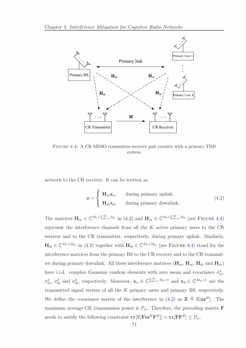
Chapter 4: Interference Mitigation for Cognitive Radio Networks
Figure 4.4: A CR MIMO transmitter-receiver pair coexists with a primary TDDsystem.
network to the CR receiver. It can be written as
z =
Hurxu, during primary uplink
Hdrxd, during primary downlink.(4.2)
The matrices Hur ∈ CMr×
∑Kk=1 Mk in (4.2) and Hut ∈ C
Mt×∑K
k=1 Mk (see Figure 4.4)
represent the interference channels from all the K active primary users to the CR
receiver and to the CR transmitter, respectively, during primary uplink. Similarly,
Hdr ∈ CMr×Mbs in (4.2) together with Hdt ∈ CMt×Mbs (see Figure 4.4) stand for the
interference matrices from the primary BS to the CR receiver and to the CR transmit-
ter during primary downlink. All these interference matrices (Hur, Hut, Hdr and Hdt)
have i.i.d. complex Gaussian random elements with zero mean and covariance σ2ur,
σ2ut, σ
2dr and σ2
dt, respectively. Moreover, xu ∈ C∑K
k=1 Mk×1 and xd ∈ CMbs×1 are the
transmitted signal vectors of all the K primary users and primary BS, respectively.
We define the covariance matrix of the interference in (4.2) as Z , E[zzH ]. The
maximum average CR transmission power is Pcr. Therefore, the precoding matrix F
needs to satisfy the following constraint tr[E[FssHFH ]] = tr[FFH ] ≤ Pcr.
71

Chapter 4: Interference Mitigation for Cognitive Radio Networks
4.3.3 Principle of SP-Based Precoding
The precoding problem for the CR transmitter is modeled as the following optimisa-
tion problem [65]
maxF
log2det
(
I+HFFHHH
σ2n
)
(4.3)
subject to tr[FFH ] ≤ Pcr (4.4)
tr[GkFFHGH
k ] ≤ Γk k = 1, . . . , L . (4.5)
In (4.5), Gk ∈ CMk×Mt is the channel matrix from the CR transmitter to the kth
primary user. Thus, the channel matrix from the CR transmitter to all primary users
becomes HHut=[GT
1 , · · · ,GTK ]
T where channel reciprocity is assumed. The constraints
on the CR transmission power and the maximum allowed interference perceived at
each primary user are given by (4.4) and (4.5), respectively.
The projected channel singular value decomposition (SVD) or P-SVD precoding has
been proposed in [65] as a suboptimal solution for the above optimisation problem. It
first projects the CR channel H onto the null space of HHut. The effective CR channel
matrix H⊥ after projection becomes [65]
H⊥ = H(I−UGUHG ) (4.6)
where UG comes from the SVD of HHut, i.e., H
Hut = VGΛ
1/2G UH
G . Then, the precoding
matrix of the CR transmitter for the effective CR channel H⊥ can be obtained as [65]
F = U⊥
[
(µI−Λ−1⊥ )+
]12 (4.7)
where U⊥ and Λ⊥ originate from the SVD of H⊥, i.e., H⊥ = V⊥Λ1/2⊥ UH
⊥ , (·)+ =
max(0, ·) and µ denotes the power level for a water-filling (WF) algorithm such that
tr[(µI−Λ−1⊥ )+] = Pcr. With perfect CSI of HH
ut, the precoding with F will completely
avoid interference to primary users.
72

Chapter 4: Interference Mitigation for Cognitive Radio Networks
In practice, HHut has to be estimated. Therefore, the SP precoding is introduced in
[68] and [69] to estimate the space UGUHG spanned by HH
ut via sensing for (4.6). The
SP precoding is composed of two phases - uplink sensing and downlink transmission
as shown in Figure 4.5.
By analogy with the multiple signal classification (MUSIC) technique [67], the signal
covariance matrix is decomposed into signal and noise subspaces to estimate UG at
the end of the sensing phase, which can be mathematically expressed as [68]
Rut =1
LS
LS∑
i=1
rut(i)rHut(i) (4.8)
= UΛUH (4.9)
= UGΛGUHG + UnΛnU
Hn . (4.10)
In (4.8), rut(i) = Hutxu(i) + n(i) is the ith received symbol at the CR transmitter,
and Rut denotes the average covariance matrix of the received symbols. An eigenvalue
decomposition (EVD) is then performed on Rut in (4.9), where Λ = diag(λ1, · · · , λMt)
is a diagonal matrix with descendingly ordered eigenvalues of Rut and U ∈ CMt×Mt
Figure 4.5: System diagram for the proposed precoding schemes.
73

Chapter 4: Interference Mitigation for Cognitive Radio Networks
contains the corresponding eigenvectors. The matrix Rut is further decomposed into
interference and noise components in (4.10) with UG and Un being the first Kp =
rank(Hut) and the remaining (Mt−Kp) columns of U, respectively, and ΛG and Λn
being their corresponding eigenvalue matrices. A rank estimate for Kp can be carried
out by using, e.g., an Akaike information criterion (AIC) or minimum description
length (MDL) estimator [72]. The sensing phase is followed by a CR transmission,
where a precoding matrix obtained from (4.7) is applied.
The merit of the SP precoding over the P-SVD approach is that no CSI is required due
to the interference space estimation in (4.8)–(4.10). However, both of the precoding
algorithms in [68] and [69] do not consider the interference from the primary network
to the CR receiver, which eventually leads to rate loss for the CR link.
4.3.4 Proposed Precoding Schemes
In this section, two enhanced precoding schemes are proposed to tackle the problem
of CR rate loss of the aforementioned SP precoding. We elaborate the CR precoding
during the primary downlink. A similar precoding for the primary uplink can be easily
obtained, which is ignored here for brevity.
When incorporating the primary-CR interference, the precoding problem for the CR
transmitter during the primary downlink can be modeled as the following optimisation
problem
maxF
log2det
(
I+HFFHHH
Z+ σ2nI
)
(4.11)
subject to tr[FFH ] ≤ Pcr (4.12)
tr[GkFFHGH
k ] ≤ Γk, k = 1, . . . , L. (4.13)
From (4.11)–(4.13), the precoding matrix for CR transmission during the downlink
can be written as [73]
Fd = Ud
[
(µdI−Λ−1d )+
]12 (4.14)
74

Chapter 4: Interference Mitigation for Cognitive Radio Networks
where µd is the power level for the WF algorithm similar to that in (4.7) and Ud is
obtained through the following EVD
UdΛdUHd = HH
⊥ (Z+ σ2I)−1H⊥
= (I−UGUHG )
HHH(Z+ σ2I)−1H(I−UGUHG ). (4.15)
It can be seen from (4.14) and (4.15) that in order to obtain the CR precoding matrix,
the interference-plus-noise covariance matrix Rur , Z+ σ2nI needs to be estimated at
the CR receiver, besides the estimation of the interference subspace UGUHG at the CR
transmitter.
4.3.4.1 Full Projection-Based Precoding
To enable the estimation of UGUHG and Rur, we propose an enhanced precoding
scheme. The system diagram for this scheme is demonstrated in Figure 4.5. Each
CR cycle consists of sensing and transmission phases as shown in Figure 4.5. We
name the CR transmission during the primary downlink/uplink as the downlink trans-
mission T1/uplink transmission T2. For T1, the space UGUHG is estimated at the CR
transmitter during the primary uplink according to (4.8)–(4.10) over LS1 symbols.
The estimation of Rur is performed at the CR receiver at the beginning of the pri-
mary downlink phase for a batch of LS2 symbols via a procedure similar to (4.8).
After obtaining these two estimates, the CR transmitter starts transmission T1 using
the precoding matrix obtained by (4.14). The uplink transmission session T2 follows
immediately after the downlink transmission T1 but right before the sensing phase
for the next CR cycle. The CR precoding matrix for T2 can be obtained by another
two sensing sessions concurrent with the sensing phase for T1. The downlink and
uplink transmissions last for LT1 and LT2 symbols, respectively. The duration of each
CR cycle should not be longer than the channel coherence time due to the block-
fading channels. The FP-based channel projection (4.6) is employed in this proposed
precoding scheme. Therefore, it is termed as FP precoding.
75
Chapter 4: Interference Mitigation for Cognitive Radio Networks
It can be seen from Figure 4.5 that the proposed FP precoding scheme shifts the
CR cycle of the SP precoding rightwards in time. By doing this, several benefits are
obtained. Firstly, introducing CR receiver sensing phases during both the primary
downlink and uplink improves the CR instantaneous throughput by incorporating the
interference-plus-noise covariance matrix into precoding, and consequently improves
the CR throughput. Secondly, shifting the CR cycle diverts part of the CR transmis-
sion from the primary downlink to the uplink which reduces the time that primary
receivers expose themselves to interference from the CR transmitter. This is benefi-
cial to the primary network, since primary users are usually more susceptible to CR
interference than the primary BS.
Theoretically, the proposed FP precoding can completely null its transmission towards
primary users when the sensing phase is long enough and the channel noise variance
is small enough. However, the interference mitigation ability of the proposed FP
precoding degrades rapidly when the CR interference-to-noise ratio (INR, σ2ut/σ
2n)
drops below a threshold. This is due to the fact that in (4.10) some components
in the noise subspace may swap with those in the interference subspace when the
noise amplitude σn is relatively larger than the interference channel gain σut. This
phenomenon is known as a subspace swap [74]. The lower bound on the probability
of the subspace swap has been investigated in [75] and [76].
For low INR, the interference subspace has a high probability to swap with the noise
subspace. When a subspace swap happens, (4.15) can be rewritten as
UdΛdUHd ≈ (I− UnU
Hn )
HHH(Z+ σ2I)−1H(I− UnUHn )
= UGUHGH
H(Z+ σ2I)−1HUGUHG (4.16)
which means that the precoding matrix Fd and HHut span the same space. Therefore,
when the CR INR is low the average interference power received at primary users can
be expressed as
IntFPl
= E[tr[HHutFdF
HdHut]] ∝ Pcrσ
2ut. (4.17)
76

Chapter 4: Interference Mitigation for Cognitive Radio Networks
This suggests that the average interference power at primary users is proportional to
the channel gain between CR and primary users at low CR INR.
When the CR INR is high, using the similar steps as in [69] the average interference
power at primary receivers becomes
IntFPh
= E[tr[HHutUd(µdI−Λ−1
d )+UHd Hut]] (4.18)
= E[tr[HHut(Ud −Ud)(µdI−Λ−1
d )+(Ud −Ud)HHut]] (4.19)
≈ E[tr[HHut(X
HHut)†NHUd(µdI−Λ−1
d )+UdHN(HH
utX)†Hut]] (4.20)
= σ2nPcrE[tr[H
Hut(X
HHut)†(HH
utX)†Hut]] (4.21)
=σ2nPcr
LS1tr[Qu] (4.22)
where (4.19) is due to HHutUd = 0; (4.20) is obtained using the fact that Ud −Ud ≈
−(XHHut)†NHUd for high INR [77] with X , [xu(1),xu(2), · · · ,xu(LS1)], and N ,
[n(1),n(2), · · · ,n(LS1)]; (4.21) is obtained due to the independence of XHHut and N
and E[NHYN] = σ2ntr[Y]I for any constant matrixY; Qu , E[xuxu
H ] in (4.22) is the
transmit covariance matrix for the primary user. An interesting fact is observed from
(4.22) that at high CR INR the average received interference at primary users does
not depend on the interference channel HHut. The average interference is proportional
to the channel noise σ2n and inversely proportional to the sensing length LS1.
4.3.4.2 Partial Projection-Based Precoding
To further improve the throughput of the CR link, the CR transmitter does not need
to fully project its transmission to the null space of the entire interference space.
Instead, it may null its transmission to a subspace partially spanning the interference
space. Based on this analysis we introduce another precoding scheme, namely, the
PP precoding.
The PP precoding works in a similar manner to the proposed FP precoding except
for the selection of the interference space. For the downlink CR precoding, the CR
transmitter first obtains Λ and U via EVD in (4.9) during uplink sensing. Then, a
77

Chapter 4: Interference Mitigation for Cognitive Radio Networks
subspace UmUHm partially spanning the interference space is obtained by choosing m
eigenvectors corresponding to the first m largest eigenvalues of Λ, where m can be
determined according to various criteria. One candidate criterion is
∑Mmin
i=m+1 λi∑m
i=1 λi≤ rt/d (4.23)
with Mmin , min(Mt,∑K
k=1Mk). We call rt/d the trivial over dominant interference
ratio (TDIR). This selection process chooses m dominant interference subchannels to
form an estimate of the interference space and ignores the other (Mmin−m) trivial ones.
When equal power is assigned to each CR antenna, rt/d stands for the maximum ratio
of the resulting and nullified interference to the primary receiver. Finally, substituting
the estimated subspace UmUHm for UGU
HG in (4.6), the precoding matrix Fd for the
downlink CR transmission is obtained via (4.14). However, we may fail to find a value
of m satisfying (4.23). In this case, the proposed FP precoding is used. The uplink
CR precoding can be performed in the similar manner as the downlink counterpart.
The joint PDF of the ordered eigenvalues λ , [λ1, λ2, · · · , λMmin] of Rut, with λ1 ≥
λ2 ≥ · · · ≥ λMmin≥ σ2
n is [78]
fλ(λ1, λ2, · · · , λMmin) =
1
PpMmin
fλ
(
λ1 − σ2n
Pp,λ2 − σ2
n
Pp, · · · , λMmin
− σ2n
Pp
)
(4.24)
wherePp is the transmission power of each primary user antenna and fλ(λ1,λ2,· · · ,λMmin)
with λ1 ≥ λ2 ≥ · · · ≥ λMminis given by
fλ(λ1, λ2, · · · , λMmin) =
∏Mmin
i=1 e−λiλMmax−Mmini
∏Mmin−1i=1
[
∏Mmin
j=i+1(λi − λj)2]
∏Mmin
i=1 (Mmax − i)!∏Mmin
i=1 (Mmin − i)!(4.25)
with Mmax , max(Mt,∑K
k=1Mk). Therefore, the probability for the occurrence of
(4.23) is
pm =
∫
S
fλ(λ1, λ2, · · · , λMmin) dλ1 dλ2 · · · dλMmin
(4.26)
where S , (λ1, λ2, · · · , λMmin)| (4.23) ∩ λ1 ≥ λ2 ≥ · · · ≥ λMmin
≥ σ2n.
In other words, for the PP precoding scheme the probabilities of using the ‘real’ PP (m
78

Chapter 4: Interference Mitigation for Cognitive Radio Networks
satisfying (4.23) exists) and using FP are pm and (1−pm), respectively. Therefore, theCR transmitter uses [(1−pm)
∑Kk=1Mk+pmm] and
∑Kk=1Mk degrees of freedom (DoF)
for interference mitigation in the PP and FP precoding schemes. Meanwhile, the DoF
for CR transmission for the PP and FP precoding are [Mt− (1−pm)∑K
k=1Mk−pmm]
and (Mt −∑K
k=1Mk), respectively. This means that compared to the proposed FP
precoding the PP precoding scheme transfers pm(∑K
i=1Mk−m) DoF from interference
mitigation to CR transmission, which leads to a higher throughput for the CR link.
It can be seen from (4.24)–(4.26) that in the large INR regime, pm is fixed for a
given noise power σ2n and Pp, i.e., the probability of the ‘real’ PP and FP does not
change with the interference channel HHut. Considering the fact from (4.22) that
at high INRs the average interference power of FP IntFPh
is fixed and the average
interference power resulting from ‘real’ PP IntPP is proportional to the square of the
interference channel gain σ2ut, the overall average interference of the PP precoding
IntPPh
= pmIntPP + (1− p
m)IntFP
his linearly proportional to σ2
ut for large INRs.
4.3.5 Numerical Results and Discussions
In this section, the performance of the proposed precoding schemes is evaluated via
simulations. We consider a scenario where a CRMIMO system coexists with a primary
TDD system which has one 2-antenna BS and two single-antenna users. Each CR node
is equipped with four antennas, i.e., Mt = Mr = 4, Mbs = 2, K = 2 andM1 = M2 = 1.
The primary network works as a downlink-broadcast and an uplink multiple-access
system. The primary BS uses perfect zero-forcing beamforming at both the primary
downlink and uplink. The transmission power of the CR and primary networks is 1.
All the results are obtained by averaging over 2000 simulation runs.
First, we evaluated the throughput of the CR system with the proposed precoding
schemes over different values of signal-to-noise ratios, SNR, σ2H/σ
2n. In Figure 4.6,
the throughputs (mutual information in (4.11) averaged over a CR cycle) of the two
proposed precoding schemes are compared with that of the SP precoding in [68] [69]
and the P-SVD precoding with perfect CSI of [65]. The system setup is as follows:
LS1 = LS2 = LT2 = 50, LT1 = 350, σ2H = σ2
ut = 1, Pcr = 1, and rt/d = 0.1. It can be
79
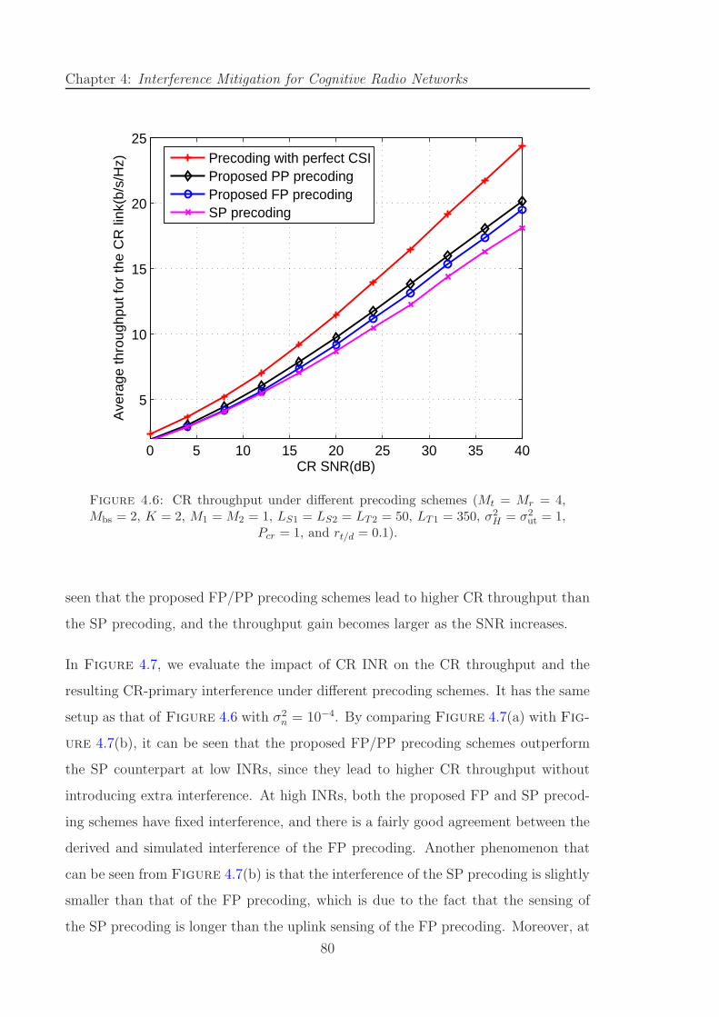
Chapter 4: Interference Mitigation for Cognitive Radio Networks
0 5 10 15 20 25 30 35 40
5
10
15
20
25
CR SNR(dB)
Ave
rage
thro
ughp
ut fo
r th
e C
R li
nk(b
/s/H
z)
Precoding with perfect CSIProposed PP precodingProposed FP precodingSP precoding
Figure 4.6: CR throughput under different precoding schemes (Mt = Mr = 4,Mbs = 2, K = 2, M1 = M2 = 1, LS1 = LS2 = LT2 = 50, LT1 = 350, σ2
H = σ2ut = 1,
Pcr = 1, and rt/d = 0.1).
seen that the proposed FP/PP precoding schemes lead to higher CR throughput than
the SP precoding, and the throughput gain becomes larger as the SNR increases.
In Figure 4.7, we evaluate the impact of CR INR on the CR throughput and the
resulting CR-primary interference under different precoding schemes. It has the same
setup as that of Figure 4.6 with σ2n = 10−4. By comparing Figure 4.7(a) with Fig-
ure 4.7(b), it can be seen that the proposed FP/PP precoding schemes outperform
the SP counterpart at low INRs, since they lead to higher CR throughput without
introducing extra interference. At high INRs, both the proposed FP and SP precod-
ing schemes have fixed interference, and there is a fairly good agreement between the
derived and simulated interference of the FP precoding. Another phenomenon that
can be seen from Figure 4.7(b) is that the interference of the SP precoding is slightly
smaller than that of the FP precoding, which is due to the fact that the sensing of
the SP precoding is longer than the uplink sensing of the FP precoding. Moreover, at
80

Chapter 4: Interference Mitigation for Cognitive Radio Networks
−40 −20 0 2017.5
18
18.5
19
19.5
20
20.5
21
21.5
22
CR INR (dB)
Ave
rage
CR
thro
ughp
ut (
b/s/
Hz)
(a)
Proposed FP precodingSP precodingProposed PP precoding
−40 −20 0 20
−45
−40
−35
−30
−25
−20
−15
−10
−5
0
CR INR (dB)
Ave
rage
inte
rfer
ence
at p
rimar
y us
er (
dBm
)
(b)
Proposed FP precodingSP precoding
Drived interference IhFP
Proposed PP precoding
Figure 4.7: (a) CR throughput and (b) resulting interference of different precodingschemes (Mt = Mr = 4, Mbs = 2, K = 2, M1 = M2 = 1,, LS = 100, LS1 = LS2 =
LT2 = 50, LT1 = 350, σ2H = 1, Pcr = 1, rt/d = 0.1, and σ2
n = 10−4).
high INRs the interference of the proposed PP precoding is linearly proportional to
the CR INR, which supports our analysis in Section 4.3.4.2.
4.4 Cross-Layer InterferenceMitigation for CRMIMO
Networks
The IM for CR MIMO systems has been investigated in Section 4.3 by proposing
two precoding schemes in physical layer. In this section, we approach the IM for CR
MIMO networks from a cross-layer perspective.
4.4.1 Related Work
Transmit precoding [64–66] is an effective IM approach to proactively mitigate CR-
primary interference for CR MIMO systems. The precoding in [64–66] assumes that
the channel information between CR and primary networks is known. But, this in-
formation is not always available to the CR network. This problem was tackled in
81

Chapter 4: Interference Mitigation for Cognitive Radio Networks
[68, 69, 79] by employing subspace technology to estimate the CR-primary channel
information before precoding. In [68] and [69], precoding schemes were proposed with
the application of the MUSIC technique to estimate the CR-primary channel infor-
mation. However, the interference from the primary network was simply ignored in
these two works during the CR precoding, which leads to CR throughput loss. In
[79], an improved precoding scheme was proposed by estimating the interference from
the primary to the CR networks and taking it into account for the CR precoding.
Therefore, the throughput of the CR network was boosted.
The aforementioned precoding techniques are prominent examples of IM techniques in
the physical layer. When multiple CR nodes share the spectrum with the primary net-
work, channel allocation of the CR network opens another door to the CR-primary IM.
Channel allocation has been extensively studied especially for cellular networks [80].
For CR networks, two adaptive channel allocation schemes were presented in [81]
based on a game theoretic framework. Therefore, it is desirable to jointly consider
the channel allocation in the MAC layer and precoding in the physical layer to mit-
igate interference from CR to primary network. This idea has already been applied
to ad hoc networks in [82] and [83], where a joint iterative channel allocation and
beamforming algorithm was proposed for interference avoidance. To the best of the
authors’ knowledge, no research attempt has been made to mitigate interference from
CR to primary networks from this perspective.
In this section, we propose two distributed cross-layer algorithms for CR MIMO sys-
tems to minimise the CR-primary interference and maximise the throughput of the
CR network. Channel allocation in the MAC layer and a sensing and projection-
based precoding scheme presented in [79] in the physical layer are jointly designed in
our work. For the case when channel information among CR nodes is available, we
present an iterative algorithm to update the channel allocation and precoding matri-
ces iteratively for all CR transmitters to balance between the CR-primary interference
and CR throughput. Alternatively, when the channel information among CR nodes
is unknown, a non-iterative algorithm together with a channel estimation scheme are
proposed to perform the joint channel allocation and precoding.
82

Chapter 4: Interference Mitigation for Cognitive Radio Networks
The remainder of this section is organised as follows. The system model and problem
formulation are given in Section 4.4.2. The cross-layer interference mitigation algo-
rithms are presented in Section 4.4.3. The performance of the proposed cross-layer
schemes are evaluated via simulations in Section 4.4.4.
4.4.2 System Model and Problem Formulation
The system model is demonstrated in Figure 4.8. Consider K pairs of CR MIMO
transmitter and receiver coexisting with a primary TDD system. Each primary and
CR node is equipped with Mp and Mc antennas, respectively. The primary system
operates over N sub-channels f1, f2, · · · , fN. Each CR pair resides in one of the
N sub-channels. The channel allocation for all active CR transmitters is denoted as
A = A1, A2, · · · , AK, where Ak ∈ f1, f2, · · · , fN, k = 1, 2, · · · , K.
Block fading channels are assumed for the primary and CR systems. In Figure 4.8,
Hi,j,Aistands for the channel matrix from the ith CR transmitter to the jth CR re-
ceiver over sub-channel Ai (i, j = 1, 2, · · · , K). We assume Hi,j,Ai∼ CN (0, σ2
H,i,j,Ai),
which means that its elements are i.i.d. circular symmetric complex Gaussian ran-
dom variables with zero mean and covariance σ2H,i,j,Ai
. Here, GU,i,Ai∼ CN (0, σ2
U,i,Ai)
and GD,j,Aj∼ CN (0, σ2
D,j,Aj) (i, j = 1, 2, · · · , K) represent the interference channel
matrices from the primary user to the ith CR transmitter during uplink and from the
primary BS to the jth CR receiver during downlink, respectively. Thus, the channel
matrix from the ith CR transmitter to the primary user is GHU,i,Ai
due to uplink/-
downlink reciprocity. These channels are quasi-static over a block of L symbols. The
channel between each CR pair Hi,i,Ai(i = 1, 2, · · · , K) is assumed to be known to
CR transmitters, but the channels between the primary and CR networks (GU,i,Ai
and GD,j,Aj) are unknown. The source information vector to transmit for the ith
CR transmitter is denoted as si (i = 1, 2, · · · , K) and E[sisHi ] = I is assumed. The
transmitted signal vectors for the primary uplink and downlink are denoted as xu and
xd, with their transmit covariance matrices being Qu , E[xuxHu ] and Qd , E[xdx
Hd ],
respectively.
83
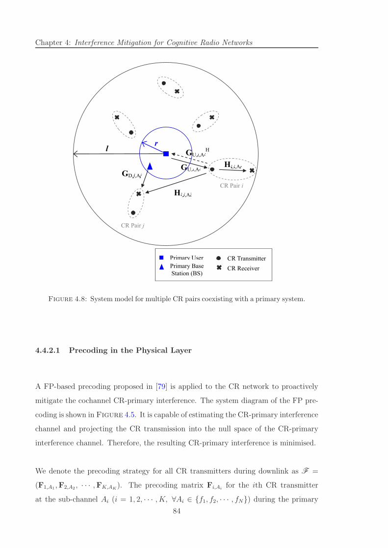
Chapter 4: Interference Mitigation for Cognitive Radio Networks
Figure 4.8: System model for multiple CR pairs coexisting with a primary system.
4.4.2.1 Precoding in the Physical Layer
A FP-based precoding proposed in [79] is applied to the CR network to proactively
mitigate the cochannel CR-primary interference. The system diagram of the FP pre-
coding is shown in Figure 4.5. It is capable of estimating the CR-primary interference
channel and projecting the CR transmission into the null space of the CR-primary
interference channel. Therefore, the resulting CR-primary interference is minimised.
We denote the precoding strategy for all CR transmitters during downlink as F =
(F1,A1 ,F2,A2 , · · · ,FK,AK). The precoding matrix Fi,Ai
for the ith CR transmitter
at the sub-channel Ai (i = 1, 2, · · · , K, ∀Ai ∈ f1, f2, · · · , fN) during the primary
84

Chapter 4: Interference Mitigation for Cognitive Radio Networks
downlink can be written as [79]
Fi,Ai= Ui
[
(µI−Λ−1i )+
]12 (4.27)
where (·)+ = max(0, ·) and µ denotes the water level for the water-filling algorithm.
Given the transmission power of each CR transmitter Pcr, we have tr[(µI−Λ−1i )+] =
Pcr. Ui and Λi are obtained through the following EVD
UiΛiUHi =(I−UG,i,Ai
UHG,i,Ai
)HHHi,i,Ai
R−1dr,i,Ai
×Hi,i,Ai(I−UG,i,Ai
UHG,i,Ai
) (4.28)
where UG,i,Aiis the matrix spanning the space of the interference channel from the
ith CR transmitter to the primary user at sub-channel Ai. It is estimated via sensing
at the ith CR transmitter during primary uplink. The estimation can be expressed as
Rut,i,Ai=
1
Ls1
Ls1∑
t=1
rut,i,Ai(t)rHut,i,Ai
(t) (4.29)
=UiΛiUHi (4.30)
=UG,i,AiΛG,i,Ai
UHG,i,Ai
+Un,i,AiΛn,i,Ai
UHn,i,Ai
(4.31)
where Rut,i,Aidenotes the average covariance matrix of the received symbols at the ith
CR transmitter over sub-channel Ai during primary uplink, rut,i,Ai(t) = GU,i,Ai
xu(t)+
n(t) is the tth received symbol at the ith CR transmitter with n(t) ∼ CN (0, σ2nI)
being the AWGN vector. EVD is then performed on Rut,i,Aiin (4.30) with Λi =
diag(λ1, λ2, · · · , λMc). UG,i,Ai
is obtained by further decomposing (4.30) into inter-
ference and noise components as shown in (4.31) where the diagonal matrix ΛG,i,Ai
consists of the Mp largest eigenvalues of Rut,i,Aiand UG,i,Ai
is the corresponding
eigenvectors.
Another component that needs to be estimated in (4.28) is Rdr,i,Ai(i = 1, 2, · · · , K)
the covariance matrix of the received signal at the ith CR receiver during primary
85

Chapter 4: Interference Mitigation for Cognitive Radio Networks
downlink over sub-channel Ai . Given a channel allocation A , it can be written as
Rdr,i,Ai=
∑
∀k:Ak=Ai,k 6=i
Hk,i,AiFk,Ai
FHk,Ai
HHk,i,Ai
+ Zi,Ai(4.32)
whereZi,Ai
= GD,i,AiQdG
HD,i,Ai
+ σ2nI, ∀i, ∀Ai ∈ f1, f2, · · · , fN. (4.33)
It can be seen from (4.32) and (4.33) that Rdr,i,Aiat the ith CR receiver consists
of three components. The first component of the right hand side of (4.32) is the
interference from cochannel CR transmitters to the ith CR receiver (cochannel CR-
CR interference). While, the interference from the primary BS and the noise constitute
the second and third components, respectively. Given A and F , the cochannel CR-
CR interference can be evaluated at each CR receiver. Zi,Aiis estimated at the ith
CR receiver during downlink sensing via a step similar to (4.29).
4.4.2.2 Channel Allocation in the MAC Layer
Besides the aforementioned precoding-based interference mitigation scheme in the
physical layer, the CR-primary interference can also be managed by carefully select-
ing the operation channel for each CR node. Therefore, we jointly consider channel
allocation in the MAC layer and the FP-based precoding in the physical layer for the
CR network to minimise the CR-primary interference and maximise the CR through-
put. It can be formulated as the following multiple criteria optimisation (MCO)
problem
minA , F
Inti, i = 1, 2, · · · , K (4.34)
maxA , F
Ii, i = 1, 2, · · · , K (4.35)
subject to tr[Fi,AiFH
i,Ai] ≤ Pcr, i = 1, 2, · · · , K (4.36)
Ai ∈ f1, f2, · · · , fN, i = 1, 2, · · · , K (4.37)
where Inti and Ii are the average interference caused by the ith CR transmitter to the
primary user and the mutual information of the ith CR link during primary downlink,
86

Chapter 4: Interference Mitigation for Cognitive Radio Networks
respectively. They are given by
Inti = GHU,i,Ai
Fi,AiFH
i,AiGU,i,Ai
(4.38)
Ii = log2 det
(
I+Hi,i,Ai
Fi,AiFH
i,AiHH
i,i,Ai
Rdr,i,Ai
)
. (4.39)
In this section, we focus on the joint channel allocation and precoding for CR trans-
mission during the primary downlink. A similar problem for the primary uplink can be
formulated by following the similar procedure of the downlink counterpart. However,
it is ignored here for brevity.
4.4.3 Joint Channel Allocation and Precoding
Scalarisation of multiple objectives is one of the most commonly used approaches [84]
for solving MCO problems. The MCO problem (4.34)–(4.37) can be scalarised into a
single objective optimisation problem as follows
minA , F
K∑
i=1
obji =
K∑
i=1
[η (Inti)− γ (Ii)] (4.40)
subject to tr[Fi,AiFH
i,Ai] ≤ Pcr, i = 1, 2, · · · , K (4.41)
Ai ∈ f1, f2, · · · , fN, i = 1, 2, · · · , K (4.42)
where η(·) and γ(·) are continuous and monotonically increasing functions. When
η(·) is convex and γ(·) is concave, the problem (4.40)–(4.42) can be transformed
into a convex optimisation problem by ignoring the cochannel CR-CR interference
when computing the CR throughput Ii in (4.39)[85]. Then, dual optimisation can be
employed to solve the convex optimisation problem as in [86].
The cochannel CR-CR interference is not always negligible for the FP-based precoding
especially when CR pairs are distributed closely to each other. Moreover, the above
optimisation problem requires to be solved in a centralised manner, which is not
desirable for CR networks. Next, we propose two distributed cross-layer algorithms
87

Chapter 4: Interference Mitigation for Cognitive Radio Networks
for solving the optimisation problem (4.40)–(4.42) without ignoring the cochannel
CR-CR interference.
4.4.3.1 Known CR-CR interference channels
We first propose a joint iterative channel allocation and precoding (JICAP) algorithm
when CR-CR interference channels are known to all CR pairs. The proposed JICAP
algorithm is depicted in Table 4.4. It works in the following manner. Firstly, all the
CR pairs carry out sensing at all sub-channels as depicted in Figure 4.5. During the
primary uplink, UG,i,Aiis estimated at each CR transmitter from (4.29)–(4.31) over
all sub-channels. Each CR receiver estimates Zi,Aiover all sub-channels during the
downlink sensing. Secondly, each CR transmitter obtains the initial precoding ma-
trices from (4.27) and (4.28) for all sub-channels by ignoring the cochannel CR-CR
interference. Finally, the channel allocation and precoding are performed iteratively.
Table 4.4: The JICAP algorithm.
1. Estimate UG,i,Aiand Zi,Ai
(∀i, ∀Ai ∈ f1, f2, · · · , fN)during uplink and downlink sensing at each CR pair.
2. Obtain initial precoding matrices Fi,Aiby ignoring cochannel
CR-CR interference for each CR transmitter (∀i, ∀Ai∈f1, f2, · · · , fN).3. Start the following iteration
For t = 1, 2, · · ·For i = 1, 2, · · · , K
Select Ai(t) to minimise the obji in (4.40).Next iUpdate A ← A1(t), A2(t), · · · , AK(t).
For i = 1, 2, · · · , KUpdate Rdr,i,Ai
according to A .Obtain Fi,Ai
(t) from (4.27)–(4.33).Next iUpdate F ← F1,A1(t),F2,A2(t), · · · ,FK,AK
(t).
Terminate when the channel allocation A converges.Next t
88
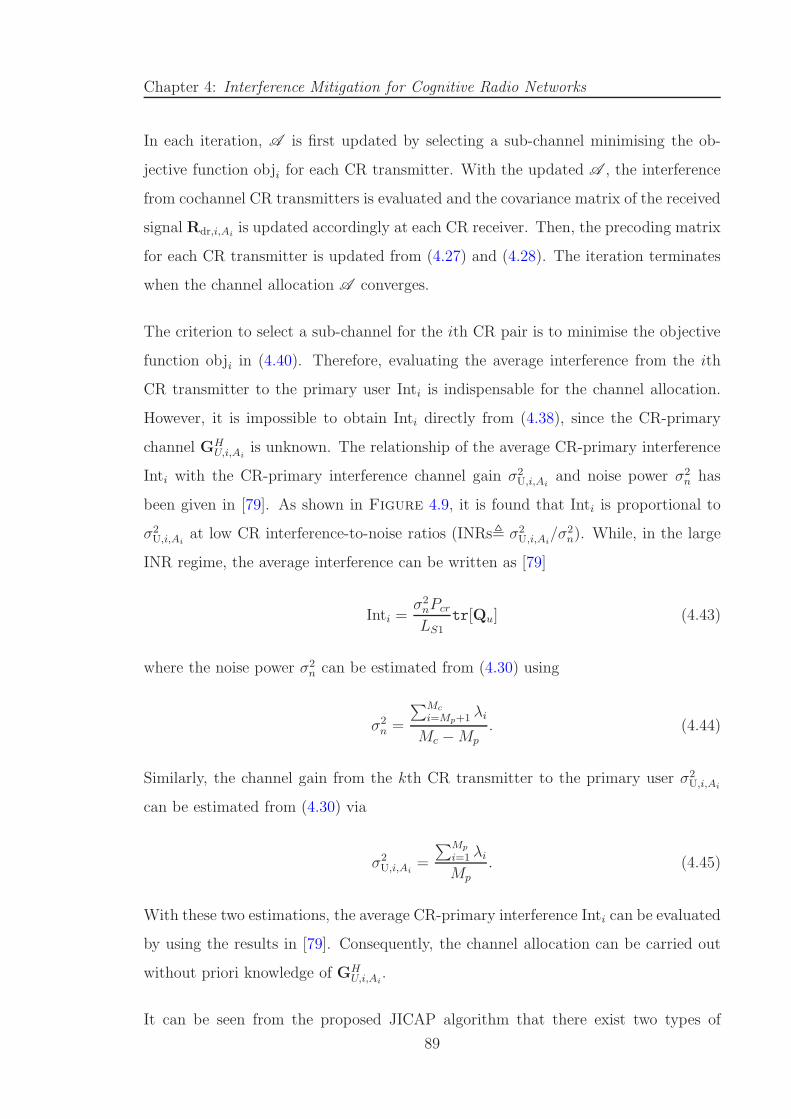
Chapter 4: Interference Mitigation for Cognitive Radio Networks
In each iteration, A is first updated by selecting a sub-channel minimising the ob-
jective function obji for each CR transmitter. With the updated A , the interference
from cochannel CR transmitters is evaluated and the covariance matrix of the received
signal Rdr,i,Aiis updated accordingly at each CR receiver. Then, the precoding matrix
for each CR transmitter is updated from (4.27) and (4.28). The iteration terminates
when the channel allocation A converges.
The criterion to select a sub-channel for the ith CR pair is to minimise the objective
function obji in (4.40). Therefore, evaluating the average interference from the ith
CR transmitter to the primary user Inti is indispensable for the channel allocation.
However, it is impossible to obtain Inti directly from (4.38), since the CR-primary
channel GHU,i,Ai
is unknown. The relationship of the average CR-primary interference
Inti with the CR-primary interference channel gain σ2U,i,Ai
and noise power σ2n has
been given in [79]. As shown in Figure 4.9, it is found that Inti is proportional to
σ2U,i,Ai
at low CR interference-to-noise ratios (INRs, σ2U,i,Ai
/σ2n). While, in the large
INR regime, the average interference can be written as [79]
Inti =σ2nPcr
LS1tr[Qu] (4.43)
where the noise power σ2n can be estimated from (4.30) using
σ2n =
∑Mc
i=Mp+1 λi
Mc −Mp
. (4.44)
Similarly, the channel gain from the kth CR transmitter to the primary user σ2U,i,Ai
can be estimated from (4.30) via
σ2U,i,Ai
=
∑Mp
i=1 λi
Mp. (4.45)
With these two estimations, the average CR-primary interference Inti can be evaluated
by using the results in [79]. Consequently, the channel allocation can be carried out
without priori knowledge of GHU,i,Ai
.
It can be seen from the proposed JICAP algorithm that there exist two types of
89

Chapter 4: Interference Mitigation for Cognitive Radio Networks
−40 −30 −20 −10 0 10 20 30
−45
−40
−35
−30
−25
−20
−15
CR INR (dB)
Ave
rage
CR
−pr
imar
y in
terf
eren
ce (
dBm
)
FP−based precodingDerived interference at high INRs
Figure 4.9: Relationship between CR INR and the average CR-primary interfer-ence (Mp = 2, Mc = 4, K = 1, LS1 = LS2 = 50, σ2
H = 1, Pcr = 1 Unit, andσ2n = 10−4).
interaction across the MAC and physical layers. On one hand, the channel allocation
A from the MAC layer is passed down to the physical layer to update the precoding
matrices. On the other hand, the precoding strategy F from the physical layer is fed
up to the MAC layer to evaluate the objective function obji for channel selection.
4.4.3.2 Unknown CR-CR interference channels
To facilitate the proposed JICAP algorithm in Section 4.4.3.1, it is obvious that the
precoding matrices Fi,Aitogether with the associated CR-CR interference channel
Hi,j,Aiare needed by the jth CR pair (i, j = 1, 2, · · · , K, ∀i 6= j) for both channel
allocation and precoding. Hereafter, we name them as effective CR-CR interference
channels Hi,j,AiFi,Ai
. However, these information is not always available to the CR
network. Various estimation techniques can be employed to perform channel esti-
mation [87], but it incurs much communication overhead for the proposed JICAP
90
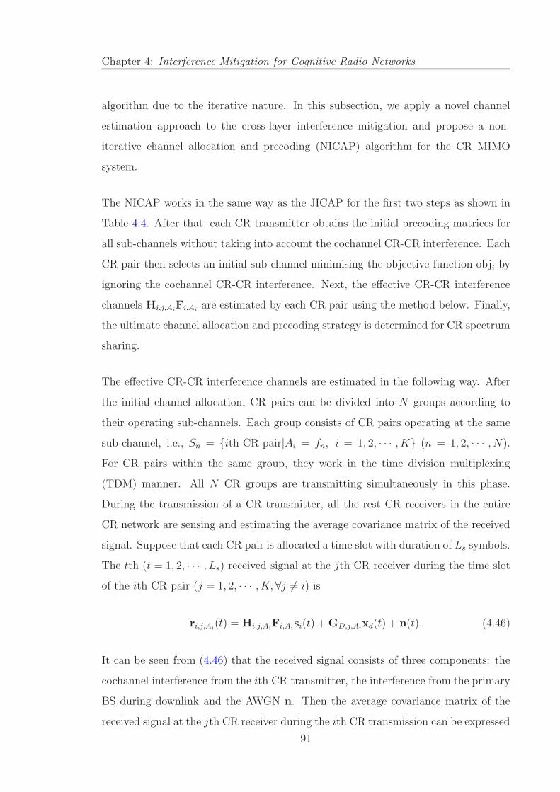
Chapter 4: Interference Mitigation for Cognitive Radio Networks
algorithm due to the iterative nature. In this subsection, we apply a novel channel
estimation approach to the cross-layer interference mitigation and propose a non-
iterative channel allocation and precoding (NICAP) algorithm for the CR MIMO
system.
The NICAP works in the same way as the JICAP for the first two steps as shown in
Table 4.4. After that, each CR transmitter obtains the initial precoding matrices for
all sub-channels without taking into account the cochannel CR-CR interference. Each
CR pair then selects an initial sub-channel minimising the objective function obji by
ignoring the cochannel CR-CR interference. Next, the effective CR-CR interference
channels Hi,j,AiFi,Ai
are estimated by each CR pair using the method below. Finally,
the ultimate channel allocation and precoding strategy is determined for CR spectrum
sharing.
The effective CR-CR interference channels are estimated in the following way. After
the initial channel allocation, CR pairs can be divided into N groups according to
their operating sub-channels. Each group consists of CR pairs operating at the same
sub-channel, i.e., Sn = ith CR pair|Ai = fn, i = 1, 2, · · · , K (n = 1, 2, · · · , N).
For CR pairs within the same group, they work in the time division multiplexing
(TDM) manner. All N CR groups are transmitting simultaneously in this phase.
During the transmission of a CR transmitter, all the rest CR receivers in the entire
CR network are sensing and estimating the average covariance matrix of the received
signal. Suppose that each CR pair is allocated a time slot with duration of Ls symbols.
The tth (t = 1, 2, · · · , Ls) received signal at the jth CR receiver during the time slot
of the ith CR pair (j = 1, 2, · · · , K, ∀j 6= i) is
ri,j,Ai(t) = Hi,j,Ai
Fi,Aisi(t) +GD,j,Ai
xd(t) + n(t). (4.46)
It can be seen from (4.46) that the received signal consists of three components: the
cochannel interference from the ith CR transmitter, the interference from the primary
BS during downlink and the AWGN n. Then the average covariance matrix of the
received signal at the jth CR receiver during the ith CR transmission can be expressed
91
Chapter 4: Interference Mitigation for Cognitive Radio Networks
as
Ri,j,Ai=
Ls∑
t=1
ri,j,Ai(t)ri,j,Ai
(t)H
(a)= Hi,j,Ai
FiFHi H
Hi,j,Ai
+GD,j,AiQdG
HD,j,Ai
+ σ2nI
(b)= Hi,j,Ai
FiFHi H
Hi,j,Ai
+ Zj,Ai(4.47)
where in (4.47), (a) is due to the fact that E[sisHi ] = I and E[xdx
Hd ] = Qd; substituting
(4.33) into (a) yields (b). Therefore, the covariance matrix of the effective CR-CR
interference channel from the ith CR transmitter to the jth CR receiver at sub-channel
Ai can be expressed as
Hi,j,AiFi,Ai
FHi,Ai
HHi,j,Ai
= Ri,j,Ai− Zj,Ai
. (4.48)
The above equation suggests that the covariance matrices of the effective CR-CR inter-
ference channels needed by the channel allocation and precoding can be obtained via
the effective CR-CR channel estimation mentioned above and the primary downlink
sensing. It is easy to understand that the average duration for the effective CR-CR
interference channel estimation phase is KLs/N . Moreover, the NICAP algorithm
works in a non-iterative manner and the effective CR-CR interference channels are
only estimated for one time. Therefore, the cross-layer communication overhead is
significantly reduced compared to that of the JICAP.
It is worth noting that compared to non-cross-layer interference mitigation schemes
both of the proposed cross-layer approaches are performed at the expense of increased
complexity due to the cross-layer consideration. In general, the complexity involved
in each proposed approach increases with the increase of CR number. Moreover, the
complexity increase of the JICAP algorithm is more obvious than that of the NICAP
due to its iterative nature.
92

Chapter 4: Interference Mitigation for Cognitive Radio Networks
4.4.4 Simulation Results
The performance of the proposed JICAP and NICAP algorithms is evaluated via
simulations in this section. In our simulations, we consider that K = 10 pairs of CR
links coexist with a primary system. The primary network operates over N = 3 sub-
channels. Each primary and CR node is equipped with Mp = 2 and Mc = 4 antennas,
respectively. The primary user locates at the origin of a 2-dimensional plane. As
demonstrated in Figure 4.8, the primary BS and all the CR pairs are uniformly
distributed around the primary user with radii r = 10m and l = 100m, respectively.
Rayleigh fading channels are assumed for the primary and the CR systems. The CR
transmission power and the noise power are set as Pcr = 1 and σ2n = 10−4. The uplink
and downlink sensing for the FP-based precoding both last for 25 symbols. The time
slot for each CR pair during the effective CR-CR channel estimation is also set to 25
symbols, i.e., Ls1 = Ls2 = Ls = 25. The objective function for the JICAP algorithm
is designed as obji = 3× 10⁵Inti − Ii.
With this setup, both the CR sum rate (mutual information) and the overall average
resulting interference perceived at the primary user are examined for the two proposed
algorithms in Figure 4.10. Each point in our simulations is obtained by averaging
over 2000 simulation runs. The performance of these two proposed algorithms is com-
pared with that of another two schemes: non-cross-layer and minimum interference
approaches. For the former approach, a random channel allocation is performed and
then used throughout the whole CR transmission phase. Its channel allocation and
precoding are performed separately and no interaction exists between the physical
and the MAC layers. Hence, it is termed as the non-cross-layer approach. While,
for the latter the channel allocation in each iteration aims at minimising the result-
ing CR-primary interference, i.e., the second criteria (4.35) for the MCO problem is
ignored.
It can be seen from Figure 4.10 that compared to the non-cross-layer approach,
the proposed JICAP and NICAP algorithms reduce the CR-primary interference and
boost the CR throughput at the same time. Therefore, the cross-layer schemes out-
perform the non-cross-layer counterpart. The minimum interference approach can
93

Chapter 4: Interference Mitigation for Cognitive Radio Networks
0 10 20 30 40 50
−11.6
−11.5
−11.4
−11.3
−11.2
Iteration numbers
CR
inte
rfer
ence
(dB
m)
Non−cross−layer approachProposed JICAP algorithmProposed NICAP algorithmMinimum interference approach
0 10 20 30 40 5030
40
50
60
70
80
Iteration numbers
CR
sum
rat
e (b
/s/H
z)
Non−cross−layer approachProposed JICAP algorithmProposed NICAP algorithmMinimum interference approach
Figure 4.10: Performance evaluation of the proposed cross-layer algorithms (r =10m, l = 100m, K = 10, N = 3, Mp = 2, Mc = 4, Ls1 = Ls2 = Ls = 25, Pcr = 1,
and σ2n = 10−4).
further reduce the CR-primary interference by compromising the CR throughput.
This suggests that the proposed cross-layer algorithms can effectively balance the in-
terference minimisation and the CR throughput maximisation. Furthermore, it can
also been seen from Figure 4.10 that the NICAP algorithm together with the pro-
posed estimation scheme for the effective CR-CR interference channels leads to similar
performance to that of the JICAP with known CR-CR interference channels.
Finally, the convergence of the proposed JICAP algorithm is evaluated in Figure 4.11
for one realisation of the primary and CR systems. We use the same setup as that
of Figure 4.10. As we can see from Figure 4.11, the channel allocation for all
10 CR pairs converges rapidly. Meanwhile, the CR sum rate converges right after
the convergence of the channel allocation. This is due to the fact that after the
channel allocation is fixed the FP-based precoding does not take long to reach the
94

Chapter 4: Interference Mitigation for Cognitive Radio Networks
0 5 10 15 20 25 30
1
2
3
Iteration numbersCha
nnel
allo
catio
n (s
ub−c
hann
els)
CR 1CR 2CR 3CR 4CR 5CR 6CR 7CR 8CR 9CR 10
0 5 10 15 20 25 3071
72
73
74
75
76
Iteration numbers
CR
sum
rate
(b/s
/Hz)
Figure 4.11: Convergence of the proposed JICAP algorithm (r = 10m, l = 100m,K = 10, N = 3, Mp = 2, Mc = 4, Ls1 = Ls2 = Ls = 25, Pcr = 1, and σ2
n = 10−4).
Nash equilibrium - a stable state where no CR links can improve their throughput by
unilaterally changing their own precoding matrices.
4.5 Chapter Summary
CR networks could lead to complex and sophisticated interference scenarios. This has
inspired our investigation on applying IM techniques to CR networks with a special
focus on mitigating the inter-network interference. We have found that a CR receiver
assisted by proper IC techniques can effectively combat primary-CR interference given
that the secondary signals have dissimilar characteristics to those of primary signals.
In addition, various IA techniques have been found to be useful for CR transmitters
95
Chapter 4: Interference Mitigation for Cognitive Radio Networks
to rigidly control their emission patterns and thereby mitigate the CR-primary in-
terference. Moreover, we have shown that hybrid IC schemes can be applied to CR
networks by combining simple IM techniques.
Then, we confine our attention to the mitigation of CR-primary interference. Two
SP precoding-based schemes, namely, FP and PP precoding, have been proposed for
CR MIMO systems to mitigate their interference to the primary network and improve
the CR throughput. These two precoding schemes are capable of estimating the CSI
of interference channels between primary and CR networks and can account for the
interference from the primary system via a novel sensing approach. Therefore, no extra
signalling is required between primary and CR systems, which consequently eases the
deployment of CR networks. The performance of the proposed precoding schemes has
been evaluated and compared with that of the existing precoding approaches. It has
been demonstrated that the FP precoding can boost the CR throughput and does not
introduce extra interference to the primary system in the low INR regime. The PP
precoding can further improve the CR throughput if the primary system can tolerate
some extra interference.
Finally, the mitigation of CR-primary interference has been investigated from a cross-
layer perspective for CR MIMO systems. A distributed iterative channel allocation
and precoding algorithm has been proposed to minimise the CR-primary interfer-
ence and maximise the CR throughput when interference channels among CR nodes
are available. While, for the scenario with unknown CR-CR interference channel in-
formation, we have proposed a non-iterative cross-layer algorithm together with an
estimation scheme for effective CR-CR interference channels. Simulation results have
demonstrated that (i) both of the proposed cross-layer algorithms outperform the
non-cross-layer approach in terms of the resulting CR-primary interference and the
CR throughput; (ii) the non-iterative algorithm achieves similar performance to the
iterative counterpart without incurring much communication overhead.
So far, the CR-primary interference has been investigated from two aspects: interfer-
ence modelling in Chapter 3 and interference mitigation in Chapter 4. Both of them
give insights into CR deployment aiming at reducing the CR-primary interference. In
96

Chapter 4: Interference Mitigation for Cognitive Radio Networks
the next chapter, we shift our attention to the study of the other type of interference
originating from CR networks, i.e., CR-CR interference.
97


Chapter 5
Interference Channel Analysis for
Spectrum-Sharing Cognitive Radio
Networks
5.1 Introduction
Besides the CR-primary interference investigated in Chapters 3 and 4, the other type
of interference from CR networks, CR-CR interference, is also worth studying. In
this chapter, we analyse the CR-CR interference channel for spectrum-sharing CR
nodes when they interfere with each other. We model the rate control in interference
systems as an MCO problem, analyse the interference channel by characterising its
resulting Pareto rate region and apply game theory to coordinate the interfering users
and solve the MCO problem. The results presented in this chapter are primarily
related to the spectrum-sharing CR networks as we look for the increase of spectrum
utilisation. They are also valid for the long-standing interference channel analysis of
other spectrum sharing networks. This is due to the fact that the underlying CR-
CR interference channel can be easily generalised into a general interference channels
regardless the working mode of the CR network. For interference-free CR networks,
the CR-CR interference channel does not differ from other interference channels apart
99

Chapter 5: Interference Channel Analysis for Spectrum-Sharing CR Networks
from the spectrum sensing prior to the spectrum exploiting. As for interference-
tolerant CR networks adopting the SP precoding delineated in Chapter 4, the effective
CR-CR interference channels become the projection of CR-CR channels into the null
space of the associated CR-primary channels. To this end, we perform the analysis
for generalised interference channels without confining it to the CR case.
We start this chapter by giving some introduction on MCO. The MCO, which is
featured by the need to simultaneously optimise multiple noncommensurable or even
incompatible objectives, has been widely used in automatic control, telecommuni-
cations, economics, and many other fields of engineering and science[88]. An MCO
problem usually admits infinite number of noninferior solutions, which form a Pareto
boundary and encompass a Pareto region [89]. A noninferior solution in the Pareto
boundary is considered to be Pareto optimal in the sense that no other solution can
improve the performance of some objectives without deteriorating other objective(s).
The characteristics of the Pareto region are of particular interest in terms of shedding
light on solving the corresponding MCO problem.
Two main processes are involved in solving the MCO problem, namely, computing
and decision making [84]. In the former process, a set of noninferior solutions for
the MCO problem is obtained, while, in the latter one, a final solution among the
noninferior solutions is determined according to certain preferences of the system.
Depending on the principle according to which these two processes interact with
each other in searching for a compromise solution, the MCO problem can be solved
using one of the following three approaches [84]: priori, posteriori and progressive
articulation of preferences. As the name suggests, the decision maker expresses its
preferences prior to the computing process in the first approach. These preferences
are often given in the form of an utility function aggregating all objectives. As for the
posteriori case, the preferences of the decision maker are not known before computing.
Thus, all the noninferior solutions for the MCO problem should be found before
decision making. Unlike the first two approaches, for the progressive articulation of
preferences, computing and decision making are performed in an alternating manner.
In each iteration, a population of noninferior solutions is maintained during computing
100

Chapter 5: Interference Channel Analysis for Spectrum-Sharing CR Networks
process; then, the decision maker chooses several suitable compromise solutions for
the computing process in next iteration to produce a new generation of noninferior
solutions. After rounds of iterations, the final solution is obtained. Evolutionary
algorithms are usually employed in this approach [90].
Among the three aforementioned approaches for solving the MCO problem, the priori
articulation of preferences is most commonly used due to its simplicity and effective-
ness. It can be further broken down into three broad classes of methods: scalarisation
of multiple objectives - the MCO problem is transformed into a single-objective op-
timisation problem by scalarising the multiple objectives into a single-valued utility
function [84]; prioritisation of multiple objectives - a certain priority is assigned to
each objective and the problem is optimised according to the priority order of its ob-
jectives [91]; goal-value method - a goal value (usually the minimum attained perfor-
mance) is assigned to each objective before optimisation to indicate its corresponding
desired level of performance [92].
The rate control problem in multi-user interference systems can be formulated as an
MCO problem. The convexity of the Pareto rate region of such MCO problem is a
desirable feature for interference systems. Various approaches have been applied to
convexify a rate region1 [93], [94]. One widely-used approach is based on the use
of a convex hull (see, for example [93]), which corresponds to the so-called time-
sharing strategies. However, the time-sharing rate boundary is achievable only in
terms of average rate rather than instantaneous rate. Another approach is based on
using orthogonal strategies (orthogonal signaling schemes), e.g., TDM and frequency
division multiplexing (FDM) [94]. Orthogonal signalling schemes significantly simplify
the MCO problem, but they usually lead to smaller achievable rate regions. The
corresponding rate loss can be significant when the interference is low [95]. Therefore,
it is desirable to analyse the convexity of the true Pareto rate region employing pure
strategy.
1When referring to rate region/boundary, we mean the Pareto rate region/boundary hereafter, ifthere is no particular other clarification.
101

Chapter 5: Interference Channel Analysis for Spectrum-Sharing CR Networks
To solve the MCO problem in multi-user interference systems, several methods have
been developed in the literature based on the widely-used priori articulation of prefer-
ences approach [84]. The most representative one is the sum-rate maximisation ( see,
for example, the sum-rate maximisation for multi-user MIMO interference systems in
[96]). The obvious drawback of this method is the lack of fairness, since the perfor-
mance of users with bad channel conditions is always sacrificed. The fairness can be
improved by weighted sum rate approaches like in [97], but it is not straightforward
to determine the weighting coefficients for all users. The preference can also be based
on proportional fairness [98], where the fairness of a user is proportional to its chan-
nel condition. Recently, game theory has been increasingly used in the rate control
and optimisation for communication systems [99]. Particularly, the NB from coop-
erative game theory has been widely used to solve the MCO problem for multi-user
interference systems. Note that NB is an effective scheme to balance the fairness of in-
dividual users and the system-level performance[100]. Representative examples in the
literature include [94] and [101] for single-input single-output (SISO), [93] and [102]
for multiple-input single-output (MISO), and [103] for MIMO interference systems.
In [103], a practical suboptimal algorithm for finding the NB solution was designed
by exploring the gradient projection method [96]. However, little research has been
done to characterise the pure strategy based NB for MIMO interference systems.
In this chapter, we apply MCO to the rate control problem in multi-user interference
systems. Specifically, we formulate the cooperative rate control of MIMO interference
systems as an MCO problem. The contribution of this chapter can be summarised as
follows.
• The Pareto rate region of the MCO problem is characterised. It is proved
that the condition that interference-plus-noise covariance matrices approach the
identity matrix is a sufficient condition for the convexity of the rate region.
Moreover, a significant implication is found that when interference is high, in-
terference mitigation techniques are preferable for convexifying the rate region.
102

Chapter 5: Interference Channel Analysis for Spectrum-Sharing CR Networks
• Various rate region convexification approaches including a multi-stage IC and a
FP precoding-based IA scheme are analysed. An achievable rate region based
on FP precoding is also given for MIMO interference systems.
• The MCO problem for rate control in multi-user MIMO interference systems is
converted to a single-objective Nash-product maximisation problem by scalaris-
ing the multiple objectives using NB. The characteristics of the NB over MIMO
interference systems such as the uniqueness of the pure-strategy NB solution
and the optimality of NB solutions resulting from different convexification ap-
proaches are studied.
In a word, this chapter gives clue on how to coordinate the operation of CR users in
spectrum-sharing CR networks. The remainder of this chapter is organised as follows.
The MCO problem and Nash-product maximisation problem for multi-user MIMO
interference systems are formulated in Section 5.2. In Section 5.3, the Pareto rate
region is characterised and various rate region convexification approaches for MIMO
interference systems are analysed. The characteristics of pure-strategy NB solution
and the optimality of NB solutions resulting from different convexification approaches
are studied in Section 5.4. The convexity of the rate region, fairness of NB, and the
existence of the FP precoding based NB solution for MIMO interference systems are
exemplified in Section 5.5 via numerical studies. Finally, conclusions are drawn in
Section 5.6.
5.2 Problem Formulation
5.2.1 MCO in MIMO Interference Systems
Consider anM-user MIMO interference system in which all users use the same wireless
channel simultaneously. The transmitter and receiver for user i (i = 1, 2, · · · ,M) are
equipped with N ti and N r
i antennas, respectively. The N ri ×1 complex baseband signal
103

Chapter 5: Interference Channel Analysis for Spectrum-Sharing CR Networks
vector received by user i can be written as [104]
yi = Hiixi +M∑
j=1,j 6=i
Hjixj + ni (i = 1, 2, · · · ,M) (5.1)
where xi ∈ CNt
i×1 is the transmitted signal vector for user i; Hii ∈ CNr
i ×Nti and
Hji ∈ CNr
i ×Ntj are channel matrices from transmitter i and transmitter j to receiver i,
respectively; we assume Hii ∼ CN (0, ρi) (i = 1, 2, · · · ,M), i.e., the elements are i.i.d.
circular symmetric complex Gaussian random variables with zero mean and variance
ρi; we also have Hji ∼ CN (0, ηji) (j = 1, 2, · · · ,M ; j 6= i); and ni ∈ CNri ×1 is the
AWGN vector of user i with zero mean and covariance matrix E[ninHi ] = I. Here, ρi
is the normalised SNR for user i and ηji is the normalised INR from transmitter j to
receiver i.
We assume that: (i) each transmitter and receiver transmits and receives symbols in-
dependently; (ii) the co-channel interference from other users is unknown and treated
as noise, i.e., no interference cancellation techniques are employed by receivers; (iii)
the channel varies slowly and it is constant during the period of each symbol trans-
mission.
The mutual information for user i can be expressed as [105]
Ii(Q) = log2 det(
I+HiiQiHHiiR
−1−i
)
, i = 1, 2, · · · ,M (5.2)
whereQi = E[xixHi ] is the Hermitian positive semi-definite transmit covariance matrix
of the input signal vector for user i, i.e., Qi 0, and
R−i = I+M∑
j=1,j 6=i
HjiQjHHji , i = 1, 2, · · · ,M (5.3)
is the interference-plus-noise covariance matrix for user i. We defineQ , Q1, · · · ,QMas a set of transmit covariance matrices. Since the transmission of each user is power
limited, the following trace constraint applies to Qi
tr[Qi] ≤ pi, i = 1, 2, · · · ,M. (5.4)
104

Chapter 5: Interference Channel Analysis for Spectrum-Sharing CR Networks
We also assume that each transmitter i has the full knowledge of the instantaneous
channels and the transmit covariance matrices of all the other transmitters.
The rate control objective in the MIMO interference system is the rate2 maximisation
for all users by optimising their transmit covariance matrices Qi (i = 1, 2, · · · ,M)
under the trace constraints given by (5.4). Therefore, rate control in the multi-user
MIMO interference system can be formulated as the following MCO problem
maxQ
Ii(Q) i = 1, 2, · · · ,M
subject to Qi 0, i = 1, 2, · · · ,M
tr[Qi] ≤ pi, i = 1, 2, · · · ,M. (5.5)
5.2.2 Scalarisation of the MCO Using NB
According to game theory, a game consists of three elements: players, strategies and
utilities [106]. Players are rational parties involved in the game. Strategies stand for
actions or behaviours taken by players. Utilities are usually defined in the form of
a certain performance metric for players. The MIMO interference system delineated
above can be modelled as a MIMO interference game, whose players are the users in
the MIMO system, the rate of each user represents the utility of the corresponding
player, and the transmit covariance matrix of each user forms the strategy space of
each player.
A game can be classified as either competitive or cooperative according to the coop-
eration scheme among players. In a competitive game, as the name suggests, all the
players compete with each other rationally and selfishly. Players neither communicate
nor cooperate with each other. A steady state in competitive games for which each
player can not improve its utility by unilaterally changing its own strategy is called
the Nash Equilibrium (NE) [106]. For a MIMO interference game, the NE can be
2Hereafter, when referring to rate, we mean mutual information (5.2).
105

Chapter 5: Interference Channel Analysis for Spectrum-Sharing CR Networks
mathematically expressed as
∀i = 1, 2, · · · ,M, Qi 0, tr[Qi] ≤ pi : Ii(Q∗i ,Q
∗−i) ≥ Ii(Qi,Q
∗−i) (5.6)
where Q∗i and Q∗
−i denote the transmit covariance matrices of the NE for user i and
for all the other users except i, respectively. The transmit covariance matrix of each
player leading to the NE can be found via iterative water filling (IWF) as [107]
Q∗i = Ui(µiI−D−1
i )+UHi , i = 1, 2, · · · ,M (5.7)
where UiDiUHi = HH
iiR−1−iHii is the EVD of HH
iiR−1−iHii, Ui (i = 1, 2, · · · ,M) is
the unitary matrix of eigenvectors, Di (i = 1, 2, · · · ,M) is a diagonal matrix of
eigenvalues, and µi denotes the power level given by IWF. It is worth noting that the
NE for MIMO interference systems is not necessarily unique [108].
Generally, the NE is not optimal from the system point of view due to its competitive
and selfish nature. Whereas, in a cooperative game, all the players negotiate with
each other prior to the game, which usually results in utility improvement [109], [110].
There exist many cooperative game-theoretic approaches. In this chapter, we restrict
our attention to the NB as one of the most popular approaches to scalarise the multiple
objectives of the MCO problem (5.5) [100].
The NB is well defined in a convex rate region [100]. In the context of the MIMO
interference game, for the case when the rate region is convex, the bargaining set, i.e.,
the set of available strategies for user i, can be expressed as
S = Qi|Qi 0, tr[Qi] ≤ pi, and Ii(Q) > INEi , i = 1, 2, · · · ,M (5.8)
where INEi is the utility of the NE for user i. It also has a disagreement point, which
is defined as the state that players resort to when the cooperation fails. Naturally,
the NE is taken as the disagreement point in NB. By applying the NB, the multiple
objectives in the MCO problem (5.5) can be scalarised. Then, the MCO problem can
106

Chapter 5: Interference Channel Analysis for Spectrum-Sharing CR Networks
be transformed into the following single-objective optimisation problem
maxQ
M∏
i=1
(Ii(Q)− INEi )
subject to Qi 0, i = 1, 2, · · · ,M
tr[Qi] ≤ pi, i = 1, 2, · · · ,M
Ii(Q) > INEi , i = 1, 2, · · · ,M . (5.9)
It is worth noting that the NB corresponds to the so-called proportional fairness and
the Nash product∏M
i=1(Ii(Q) − INEi ) is converted to the rate product of all users
when INEi = 0, ∀i. An intuitive explanation of the above optimisation problem is
that the NB introduces a cooperation scheme among all MIMO users and regulates
their transmissions by optimising transmit covariance matrices under the power con-
straints (5.9). On one hand, it guarantees that the utility of each MIMO user is not
less than the one given by the NE. On the other hand, it maximises the Nash product
of the whole MIMO system. Therefore, it provides a trade off between the fairness
requirements to individual users and the overall performance of the whole system.
In the sequel, we first characterise the Pareto rate region of the MIMO interference sys-
tems and investigate interference mitigation-based rate region convexification schemes
when the rate region is non-convex. An achievable rate region for MIMO interference
system is given as well. Then, we study several characteristics of the NB in MIMO
interference systems such as the uniqueness of the pure-strategy NB solution and the
optimality of different NB solutions.
107
Chapter 5: Interference Channel Analysis for Spectrum-Sharing CR Networks
5.3 Rate Region Characterisation and Convexifi-
cation
5.3.1 Convexity of Pareto Rate Region
The convexity of the rate region is a desirable feature for multi-user interference sys-
tems. Its immediate merit is that it usually yields larger rate region compared to
a nonconvex one. More importantly, the convexity of the rate region is a necessary
condition to ensure the convexity of rate control/optimisation problem. It simplifies
the MCO problem and makes it solvable and practically realisable. In the context of
the MIMO interference systems, we first investigate the convexity of the true Pareto
rate region using pure strategies, which treat interference as noise and do not em-
ploy any other interference management mechanisms. The true Pareto rate region is
both achievable in terms of instantaneous rate and usually larger than the orthogonal
signaling-based counterpart in low interference cases [95]. We derive the following
sufficient condition ensuring the convexity of its rate region.
Proposition1 : If the interference-plus-noise covariance matrices R−i → I (i =
1, 2, · · · , M), the Pareto rate region of the MIMO interference system is convex.
It is straightforward that the condition that utility functions Ii(Q) (i = 1, 2, · · · ,M)
in (5.2) are concave over Q is sufficient for the convexity of the rate region for MIMO
interefrence system. We can prove that the uitility functions are concave under the
condition that interference-plus-noise covariance matrices approach I. Thus, this con-
dition is also sufficient for the convexity of the rate region. The detailed proof is
provided in Appendix F.
The condition that R−i → I means that∑
j 6=iHjiYjHHji → 0. This corresponds to
the condition that INRs ηji (i, j = 1, 2, · · · ,M, j 6= i) in (5.1) are sufficiently small.
Hence, the immediate implication of Proposition 1 is that the rate region is convex
when the interference is low.
108

Chapter 5: Interference Channel Analysis for Spectrum-Sharing CR Networks
The rate region of interference systems is not always convex. There exist three broad
approaches to convexify a non-convex rate region.
• Convex hull - the most direct approach for rate region convexification. It stems
from the time-sharing signalling of extremity points on the rate boundary, where
all users agree to use one set of transmitting strategies for certain fraction of
time and to use the other set of strategies during the rest of the time (see, for
example [93]). Therefore, the time-sharing signalling fills the ‘depressions’ of the
rate region and make it convex. However, the rate region due to time-sharing
signalling is only achievable in terms of the average rate (over time). Thus, the
rate region of convex hull is not always achievable in terms of instantaneous
rate [93].
• Orthogonal signalling - the most commonly used approach to convexify a rate
region. In this case, users agree to split the radio resource (time or bandwidth)
into several orthogonal parts and each user uses one part only. TDM and FDM
are two prominent examples of orthogonal signalling. It worth noting that time
sharing involves in both TDM and convex hull. TDM distinguishes itself from
the convex hull in the sense that the former is pure time-sharing signalling
among single-user operation points. However, for the latter the time-sharing
signalling is only used to fill the ‘depressions’ of the rate region as shown in
Figure 5.1. The orthogonal signalling significantly simplifies the MCO problem
of rate control, but the associated rate loss may be significant [95]. This is due to
the fact that orthogonalisation completely removes interference from interfering
users, but it also reduces the radio resource available to each user compared to
that of the pure strategy.
• Interference mitigation- besides the convex hull and orthogonal signalling,
Proposition 1 suggests that reducing interference for each user can also make
the rate region convex. Therefore, various interference mitigation techniques are
applicable to convexify the rate region. Interference mitigation can be mainly
divided into two categories according to their applicability: (i) interference can-
cellation at the receiver and (ii) interference avoidance at the transmitter.
109
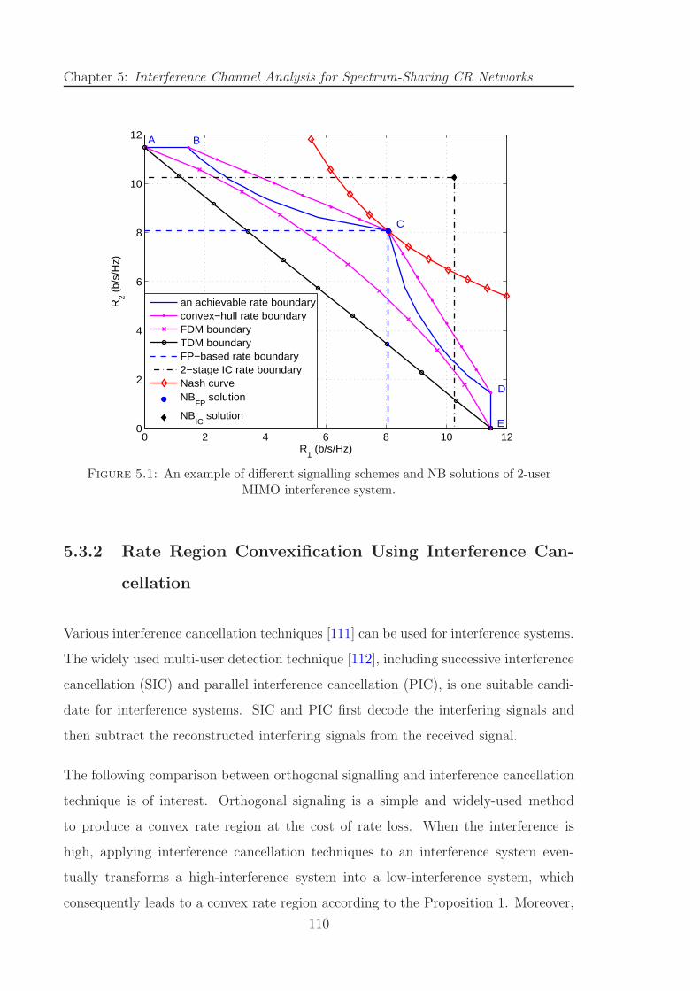
Chapter 5: Interference Channel Analysis for Spectrum-Sharing CR Networks
0 2 4 6 8 10 120
2
4
6
8
10
12
R1 (b/s/Hz)
R2 (
b/s/
Hz)
an achievable rate boundaryconvex−hull rate boundaryFDM boundaryTDM boundaryFP−based rate boundary2−stage IC rate boundaryNash curveNB
FP solution
NBIC
solution
A B
C
E
D
Figure 5.1: An example of different signalling schemes and NB solutions of 2-userMIMO interference system.
5.3.2 Rate Region Convexification Using Interference Can-
cellation
Various interference cancellation techniques [111] can be used for interference systems.
The widely used multi-user detection technique [112], including successive interference
cancellation (SIC) and parallel interference cancellation (PIC), is one suitable candi-
date for interference systems. SIC and PIC first decode the interfering signals and
then subtract the reconstructed interfering signals from the received signal.
The following comparison between orthogonal signalling and interference cancellation
technique is of interest. Orthogonal signaling is a simple and widely-used method
to produce a convex rate region at the cost of rate loss. When the interference is
high, applying interference cancellation techniques to an interference system even-
tually transforms a high-interference system into a low-interference system, which
consequently leads to a convex rate region according to the Proposition 1. Moreover,
110

Chapter 5: Interference Channel Analysis for Spectrum-Sharing CR Networks
interference cancellation removes the interference perceived at receivers, but unlike
orthogonal signaling the radio resource (time, bandwidth) available to each user for
interference cancellation remains the same as for pure strategy. Therefore, the follow-
ing remark about the practical significance of the rate region convexification can be
made.
Remark 1: When the interference is high, interference cancellation techniques out-
perform orthogonal signalling techniques for convexifying a rate region in the sense
that they lead to a convex rate region of a larger size.
We can obtain the immediate conclusion from Remark 1 that interference cancellation
ensures the uniqueness of NB solution, meanwhile, the interference cancellation based
NB (NBIC) solution has larger user rates than the orthogonal signaling based NB
solution.
As a special case, we propose a multi-stage interference cancellation technique for
a 2-user MIMO interference systems. The generalisation to the multi-user case is
straightforward and it is omitted here for brevity. It is worth noting that our objec-
tive is to demonstrate the advantages of the interference cancellation over orthogonal
signalling for the multicriteria optimisation via NB rather than considering practically
appealing interference cancellation designs.
To design our interference cancellation technique, it is required that both receivers
cooperate with each other and perform multi-stage interference cancellation as follows.
First, the receivers of users 1 and 2 decode their signals of interest and pass them to
the receivers of users 2 and 1, respectively. Using (5.1), the decoded signals from
receivers of users 1 and 2 in the first stage of interference cancellation can be written
as:
x(1)1 = H−1
11 y1 (5.10)
x(1)2 = H−1
22 y2 (5.11)
where x(1)i (i = 1, 2) are the decoded signals at the receivers of users 1 and 2 in the first
stage of the interference cancellation procedure. Second, after receiving the decoded
111
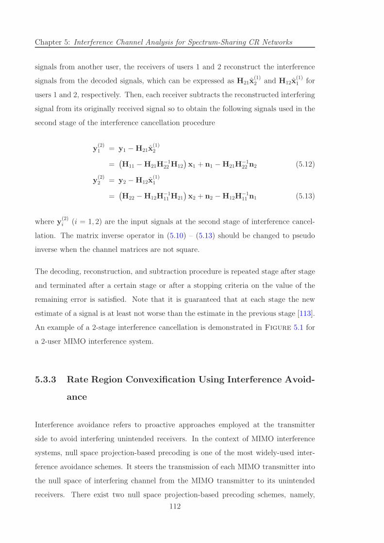
Chapter 5: Interference Channel Analysis for Spectrum-Sharing CR Networks
signals from another user, the receivers of users 1 and 2 reconstruct the interference
signals from the decoded signals, which can be expressed as H21x(1)2 and H12x
(1)1 for
users 1 and 2, respectively. Then, each receiver subtracts the reconstructed interfering
signal from its originally received signal so to obtain the following signals used in the
second stage of the interference cancellation procedure
y(2)1 = y1 −H21x
(1)2
=(
H11 −H21H−122 H12
)
x1 + n1 −H21H−122 n2 (5.12)
y(2)2 = y2 −H12x
(1)1
=(
H22 −H12H−111 H21
)
x2 + n2 −H12H−111 n1 (5.13)
where y(2)i (i = 1, 2) are the input signals at the second stage of interference cancel-
lation. The matrix inverse operator in (5.10) – (5.13) should be changed to pseudo
inverse when the channel matrices are not square.
The decoding, reconstruction, and subtraction procedure is repeated stage after stage
and terminated after a certain stage or after a stopping criteria on the value of the
remaining error is satisfied. Note that it is guaranteed that at each stage the new
estimate of a signal is at least not worse than the estimate in the previous stage [113].
An example of a 2-stage interference cancellation is demonstrated in Figure 5.1 for
a 2-user MIMO interference system.
5.3.3 Rate Region Convexification Using Interference Avoid-
ance
Interference avoidance refers to proactive approaches employed at the transmitter
side to avoid interfering unintended receivers. In the context of MIMO interference
systems, null space projection-based precoding is one of the most widely-used inter-
ference avoidance schemes. It steers the transmission of each MIMO transmitter into
the null space of interfering channel from the MIMO transmitter to its unintended
receivers. There exist two null space projection-based precoding schemes, namely,
112
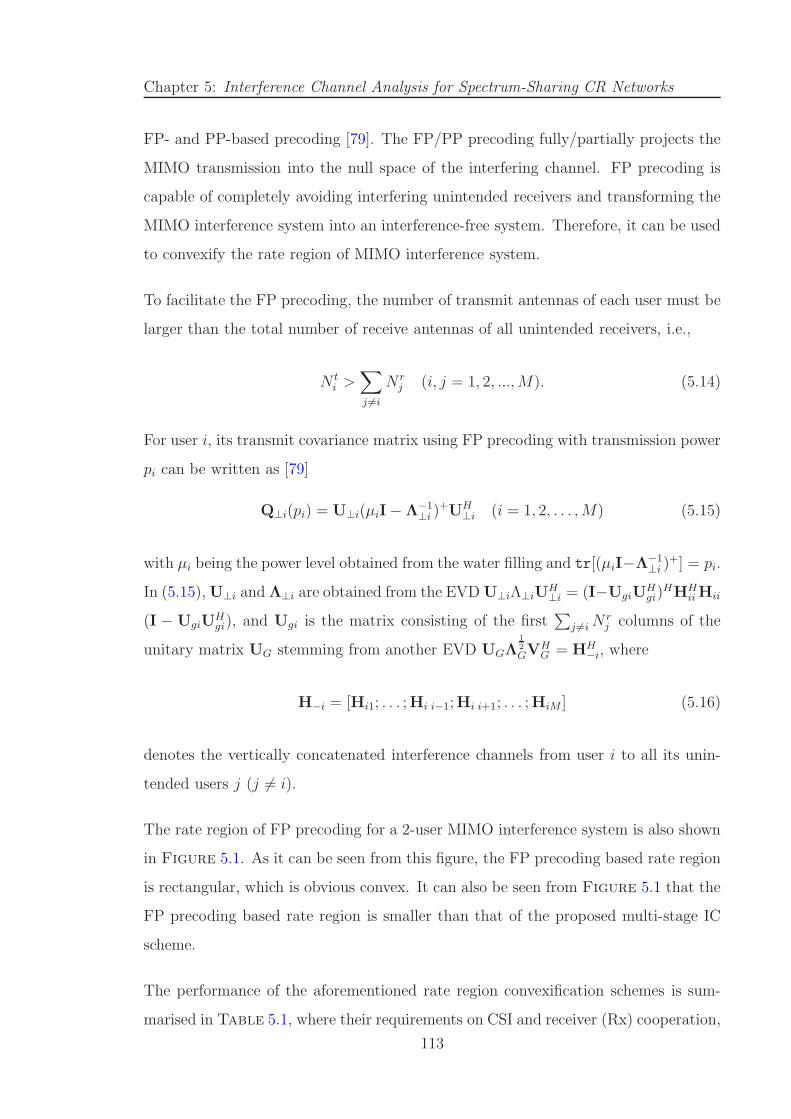
Chapter 5: Interference Channel Analysis for Spectrum-Sharing CR Networks
FP- and PP-based precoding [79]. The FP/PP precoding fully/partially projects the
MIMO transmission into the null space of the interfering channel. FP precoding is
capable of completely avoiding interfering unintended receivers and transforming the
MIMO interference system into an interference-free system. Therefore, it can be used
to convexify the rate region of MIMO interference system.
To facilitate the FP precoding, the number of transmit antennas of each user must be
larger than the total number of receive antennas of all unintended receivers, i.e.,
N ti >
∑
j 6=i
N rj (i, j = 1, 2, ...,M). (5.14)
For user i, its transmit covariance matrix using FP precoding with transmission power
pi can be written as [79]
Q⊥i(pi) = U⊥i(µiI−Λ−1⊥i )
+UH⊥i (i = 1, 2, . . . ,M) (5.15)
with µi being the power level obtained from the water filling and tr[(µiI−Λ−1⊥i )
+] = pi.
In (5.15),U⊥i and Λ⊥i are obtained from the EVDU⊥iΛ⊥iUH⊥i = (I−UgiU
Hgi)
HHHiiHii
(I − UgiUHgi), and Ugi is the matrix consisting of the first
∑
j 6=iNrj columns of the
unitary matrix UG stemming from another EVD UGΛ12GV
HG = HH
−i, where
H−i = [Hi1; . . . ;Hi i−1;Hi i+1; . . . ;HiM ] (5.16)
denotes the vertically concatenated interference channels from user i to all its unin-
tended users j (j 6= i).
The rate region of FP precoding for a 2-user MIMO interference system is also shown
in Figure 5.1. As it can be seen from this figure, the FP precoding based rate region
is rectangular, which is obvious convex. It can also be seen from Figure 5.1 that the
FP precoding based rate region is smaller than that of the proposed multi-stage IC
scheme.
The performance of the aforementioned rate region convexification schemes is sum-
marised in Table 5.1, where their requirements on CSI and receiver (Rx) cooperation,
113

Chapter 5: Interference Channel Analysis for Spectrum-Sharing CR Networks
implementation complexity and the size of resultant rate region are compared.
Table 5.1: Comparison of various rate region convexification schemes
CSI Rx cooperation Complexity Rate region size
TDM not required not required low smallFDM not required not required low medium
Multi-stage IC required required high largeFP-based IA required not required medium medium
5.3.4 Rate Region Characterisation
In what follows, we characterise the rate region for MIMO interference systems sat-
isfying (5.14) by giving an achievable rate region. We start with a 2-user MIMO
system. Its rate boundary can be obtained by finding the rate tuple (R1,maxQ(I2)).
Given a rate R1 for user 1, the corresponding rate for user 2 R2 on the rate boundary
is the maximum rate which can be achieved by user 2. This can be expressed as the
following optimisation problem
maxQ
R2 = I2(Q)
subject to I1(Q) = R1,
Qi 0, i = 1, 2
tr[Qi] ≤ pi, i = 1, 2. (5.17)
The largest R2 on the whole rate boundary can be achieved when (i) there is no
interference from user 1 to user 2, i.e., user 1 adopts the FP precoding with transmit
covariance matrix Q⊥1, and (ii) user 2 employs the maximum rate precoding with the
following transmit covariance matrix and full-power transmission
QMR2(p2) = UMR2(µ2I−Λ−1MR2
)+UHMR2
(5.18)
where UMR2 and ΛMR2 come from the EVD UMR2ΛMR2UHMR2
= HH22H22. Therefore,
an achievable rate boundary can be obtained as follows.
114

Chapter 5: Interference Channel Analysis for Spectrum-Sharing CR Networks
• For I1(Q⊥1(0),QMR2(p2))≤R1≤I1(Q⊥1(p1),QMR2(p2)), where Ii(Q1(p1),Q2(p2))
denotes the rate of user i when users 1 and 2 adopt the transmit covariance ma-
trices Q1 with Q2 with transmission power p1 and p2, R2 can achieve its largest
rate. We denote this part of rate boundary as R1. Then, we have
R1 : 0 ≤ R1 ≤ I1(Q⊥1(p1),QMR2(p2)) (5.19)
R2 = log2 det(
I+H22QMR2(p2)HH22
)
=∑
k
(
log2(p2λMR2k )
)+.
The second equality for R2 in (5.19) is obtained according to [114], λMRin (i =
1, 2, . . . ,M ; n = 1, 2, . . . , min(N ti , N
ri )) is the nth diagonal element of the eigen-
value matrix ΛMRi, and the operator
∑
k(xk)+ stands for the sum of xk with
k ∈ n|pi − 1/λMRin > 0. It is easy to understand that R1 coincides with the
boundary of the Pareto rate region. In Figure 5.1, the the line AB corresponds
to R1 where user 1 uses the FP precoding and sweeps its transmission power
form 0 to p1, and user 2 adopts the maximum rate precoding with full-power
transmission.
• At point B in Figure 5.1, R1 cannot be further improved along the line of AB
since user 1 is transmitting at full power. However, if user 2 splits some of the
transmission power for FP precoding, the interference perceived at receiver 1
caused by user 2 will reduce. Consequently, R1 can be further improved. Then,
we have the second part of the achievable rate boundary
R2 : R1 = log2 det
I+H11Q⊥1(p1)H
H11
H21 [τQ⊥2(p2) + (1− τ)QMR2(p2)]HH21
(5.20)
R2 = log2 det
I+H22 [τQ⊥2(p2) + (1− τ)QMR2(p2)]HH22
(0 ≤ τ ≤ 1).
It worth noting that R2 is one of the achievable rate boundaries, which is not
necessarily the Pareto rate boundary. In Figure 5.1, the curve BC depicts R2
where user 1 still uses FP precoding with full power and the transmit covariance
matrix for user 2 is the convex combination of FP precoding and maximum rate
precoding.
115

Chapter 5: Interference Channel Analysis for Spectrum-Sharing CR Networks
• Using the symmetry of the previous results, the other two parts of the achievable
rate boundary R3 and R4, which are respectively symmetric to R2 and R1, can
be written as
R3 : R1 = log2 det
I+H11 [(1− τ)Q⊥1(p1) + τQMR1(p1)]HH11
(5.21)
R2 = log2 det
I+H22Q⊥2(p2)H
H22
H12 [(1− τ)Q⊥1(p1) + τQMR1(p1)]HH12
(0 ≤ τ ≤ 1).
R4 : R1 = log2 det(
I+H11QMR1(p1)H
H11
)
=∑
k
(
log2(p1λMR1k )
)+
I2(QMR1(p1);Q⊥2(p2)) ≥ R2 ≥ 0.
Note that the achievable rate boundaries R3 and R4 are obtained by inter-
changing the index of the transmit covariance matrices from R2 and R1. In
Figure 5.1, the curve CD and line DE correspond to R3 and R4, respectively.
Therefore, the achievable rate boundary for the 2-user MIMO interference sys-
tem satisfying (5.14) is R = R1 ∪ R2 ∪ R3 ∪ R4.
An achievable rate region for the case of 3-user is illustrated in Figure 5.2. The
FDM based rate region is also plotted in this figure for comparison. The achievable
rate boundary consists of the following two types of 2-dimensional hypersurfaces:
• The plane ABCD is obtained when user 1 adopts the full-power maximum rate
precodingQMR1(p1) and the other two users employ the FP precoding and sweep
their transmission power from 0 to pi, i.e., Q⊥i(τipi) (i = 2, 3; τi ∈ [0, 1]). We
can get another two planes EFGH and IJKL by the symmetry of interchanging
the index of Q1, Q2 and Q3 of the plane ABCD.
• The surfaceBCOMcorresponds tothe operation strategy setofQ⊥1(p1),Q⊥2(τ2p2),
τQMR3(p3) + (1 − τ)Q⊥3(p3) (τ, τ2 ∈ [0, 1]). Another five similar surfaces
(DCON, EFOM, GFOP, LIOP, and JION) can be obtained by interchanging
the index of the transmit covariance matrices of the surface BCOM.
By induction, an achievable rate boundary for n-user can be generalised as follows.
For an n-user MIMO interference channel satisfying (5.14), one of the achievable rate
116

Chapter 5: Interference Channel Analysis for Spectrum-Sharing CR Networks
0
5
10
150 5 10 15
0
5
10
15
R2 (b/s/Hz)
R1 (b/s/Hz)
R3 (b
/s/H
z)
A
C
D
B
M
E F
H G
O
N
P
I
J
L
K
Figure 5.2: An achievable rate region for a 3-user MIMO interference system.
boundaries can be characterised by the following two types of hypersurfaces of n− 1
dimensions.
• One user (C1n) uses full-power maximum rate precodingQMRi
(pi) (i = 1, 2, · · · , n).All the other users adopt varying-power FP precoding, i.e., Q⊥j
(τjpj)(j 6= i, τj ∈[0, 1]).
• One user (C1n) uses the convex combinational precoding strategy τQMRi
(pi) +
(1− τ)Q⊥i(pi) (τ ∈ [0, 1], i = 1, 2, · · · , n). Another user among the remaining
n − 1 users (C1n−1) adopts the full-power FP precoding Q⊥j
(pj)(j 6= i). All
the rest users employ varying-power FP precoding Q⊥k(τkpk)(k 6= i, k 6= j, τk ∈
[0, 1]). Thus, the total number of hypersurfaces of these two types aggregate to
C1n + C1
nC1n−1 = n+ n(n− 1) = n2.
117

Chapter 5: Interference Channel Analysis for Spectrum-Sharing CR Networks
5.4 Characterisation of Different NB Solutions
5.4.1 Uniqueness of Pure-Strategy NB Solution
It is straightforward to see that the optimisation problem given by (5.9) is identical
to
maxQ
ln
(
lnM 2
M∏
i=1
(
Ii(Q)− INEi
)
)
subject to Qi 0, i = 1, 2, · · · ,M
tr[Qi]− pi ≤ 0, i = 1, 2, · · · ,M
INEi − Ii(Q) < 0, i = 1, 2, · · · ,M . (5.22)
Note that (5.22) is a convex optimisation problem if and only if its objective function
is concave and its constraint set is convex [85].
Proposition 2 : When the interference-plus-noise covariance matrices R−i → I (i =
1, 2, · · · ,M) , the optimisation problem (5.22) is a convex problem.
This proposition has been proved in Appendix G by showning that the condition that
the interference-plus-noise covariance matrices R−i approach I is sufficient for both
the concavity of the objective function in (5.22) and the convexity of its constraint
set.
From Proposition 2, the following corollary can be obtained.
Corollary 1: When the NE is not in the Pareto rate boundary, the condition that the
interference-plus-noise covariance matrices R−i approach I, is the sufficient condition
for the uniqueness of the pure-strategy NB solution of MIMO interference systems.
Proof. The interference-plus-noise covariance matrices R−i approaching I can ensure
the convexity of the rate region (see Proposition 1) on which the NB is defined. Inter-
estingly, it also guarantees the uniqueness of the NE in MIMO interference systems
118
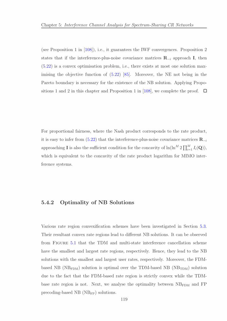
Chapter 5: Interference Channel Analysis for Spectrum-Sharing CR Networks
(see Proposition 1 in [108]), i.e., it guarantees the IWF convergences. Proposition 2
states that if the interference-plus-noise covariance matrices R−i approach I, then
(5.22) is a convex optimisation problem, i.e., there exists at most one solution max-
imising the objective function of (5.22) [85]. Moreover, the NE not being in the
Pareto boundary is necessary for the existence of the NB solution. Applying Propo-
sitions 1 and 2 in this chapter and Proposition 1 in [108], we complete the proof.
For proportional fairness, where the Nash product corresponds to the rate product,
it is easy to infer from (5.22) that the interference-plus-noise covariance matrices R−i
approaching I is also the sufficient condition for the concavity of ln(lnM 2∏M
i=1 Ii(Q)),
which is equivalent to the concavity of the rate product logarithm for MIMO inter-
ference systems.
5.4.2 Optimality of NB Solutions
Various rate region convexification schemes have been investigated in Section 5.3.
Their resultant convex rate regions lead to different NB solutions. It can be observed
from Figure 5.1 that the TDM and multi-state interference cancellation scheme
have the smallest and largest rate regions, respectively. Hence, they lead to the NB
solutions with the smallest and largest user rates, respectively. Moreover, the FDM-
based NB (NBFDM) solution is optimal over the TDM-based NB (NBTDM) solution
due to the fact that the FDM-based rate region is strictly convex while the TDM-
base rate region is not. Next, we analyse the optimality between NBFDM and FP
precoding-based NB (NBFP) solutions.
119

Chapter 5: Interference Channel Analysis for Spectrum-Sharing CR Networks
The NBFP solution for user i can be expressed as
RNBFPi = log2 det
(
I+HiiQ⊥i(pi)H
Hii
)
= maxQilog2 det
I+Hii
[
I−HH−i(H−iH
H−i)
−1H−i
]
Qi
×[
I−HH−i(H−iH
H−i)
−1H−i
]HHH
ii
=
Nti−
∑
j 6=i Nri
∑
k=1
(
log2(piλ⊥k ))+
, (5.23)
where λ⊥k (k = 1, 2, · · · , N t
i−∑
j 6=iNri ) are the eigenvalues of the user i’s effective chan-
nel matrix after projectionHii
[
I−HH−i(H−iH
H−i)
−1H−i
][
I−HH−i(H−iH
H−i)
−1H−i
]HHH
ii .
The second equality in (5.23) is obtained by interpreting the FP precoding as an op-
timal precoding of the effective channel matrix after null-space projection.
The rate of user i employing FDM when using ti(ti ∈ [0, 1]) fraction of the spectrum
can be written as
RFDMi (ti) = ti log2 det
(
I+HiiQMRi
(pi)HHii
tiI
)
= ti
Nri
∑
k=1
(
log2(piλMRi
ti)
)+
. (5.24)
Let ti∑Nr
i
k=1
(
log2(piλMRi
ti))+
= RNBFPi , we can use the following criteria to determine
the optimality of NBFP and NBFDM solutions:
• when∑M
i=1 ti > 1 the NBFP solution outperforms the FDM-based counterpart;
• when∑M
i=1 ti < 1 the NBFDM solution is optimal over the NBFP solution.
120

Chapter 5: Interference Channel Analysis for Spectrum-Sharing CR Networks
5.5 Numerical Studies
5.5.1 Convexity of the Rate Region
Proposition 1 in Section 5.3 provides the sufficient condition which guarantees the
convexity of the rate region for MIMO interference systems. Unlike Proposition 1
where the interference-plus-noise covariance matrices and then INRs are interpreted
in a qualitative manner, in this subsection we investigate the impact of the INRs
on the convexity of the rate region quantitatively via numerical studies. Consider a
2-user Rayleigh fading MIMO interference system with parameters σ = 1 and N ti =
N ri = 2 (i = 1, 2). We examine the probability that the rate region is convex for
different values of signal-to-interference ratio (SIR). It can be seen from Figure 5.3
that when the SNR is -10, 0 and 10 dB, the SIR should be at least 10, 15 and 20 dB,
respectively, to ensure that the rate region is convex. Two trends can be observed from
Figure 5.3: (i) as the SIR increases, i.e., as the INR decreases while the SNR is fixed,
the probability that the rate region is convex increases; (ii) as the SNR increases, the
SIR needs to increase as well to retain the probability that the rate region is convex.
5.5.2 Fairness of the NB
NB is a bargaining approach which balances the individual fairness and system-level
efficiency. The fairness of the NB is guaranteed by the fact that its resultant utility
for each user is not less than that of the NE, which is considered as a relatively fair
approach due to its selfish and competitive nature. In this subsection, we study the
fairness of the NB solution and compare it with other bargaining approaches. The
following bargaining solutions from [115] are taken as the benchmark for comparison:
• Egalitarian solution: It is an absolutely fair solution with identical rate for each
user.
• Kalai-Smorodinsky (K-S) solution: It results in utilities proportional to their
maximal achievable rates.
121
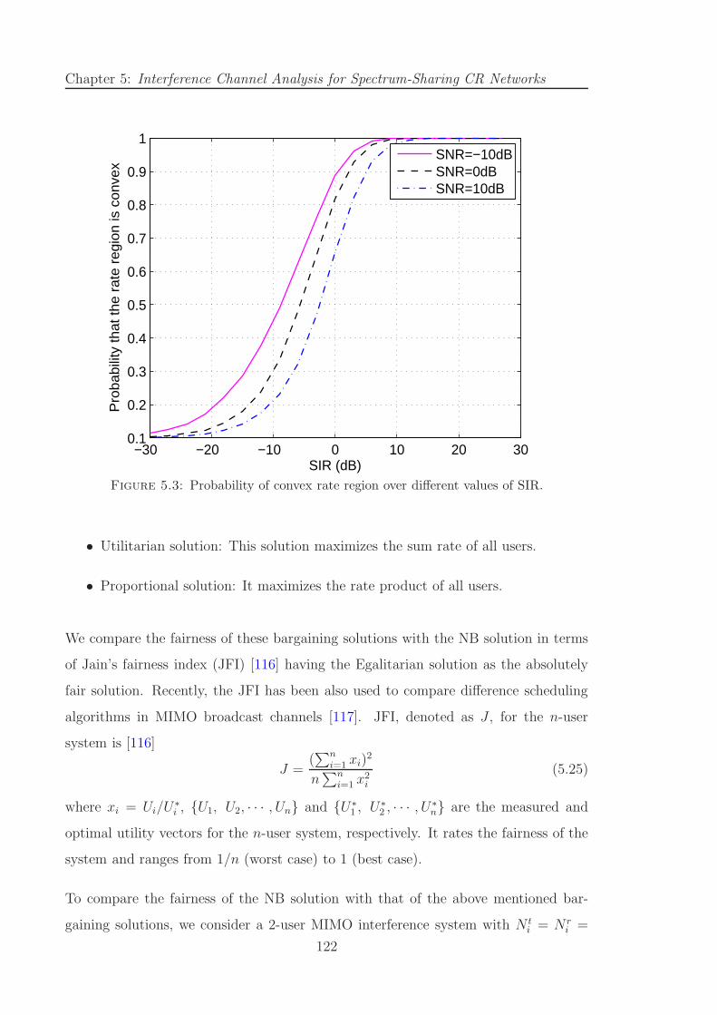
Chapter 5: Interference Channel Analysis for Spectrum-Sharing CR Networks
−30 −20 −10 0 10 20 300.1
0.2
0.3
0.4
0.5
0.6
0.7
0.8
0.9
1
SIR (dB)
Pro
babi
lity
that
the
rate
reg
ion
is c
onve
x
SNR=−10dBSNR=0dBSNR=10dB
Figure 5.3: Probability of convex rate region over different values of SIR.
• Utilitarian solution: This solution maximizes the sum rate of all users.
• Proportional solution: It maximizes the rate product of all users.
We compare the fairness of these bargaining solutions with the NB solution in terms
of Jain’s fairness index (JFI) [116] having the Egalitarian solution as the absolutely
fair solution. Recently, the JFI has been also used to compare difference scheduling
algorithms in MIMO broadcast channels [117]. JFI, denoted as J , for the n-user
system is [116]
J =(∑n
i=1 xi)2
n∑n
i=1 x2i
(5.25)
where xi = Ui/U∗i , U1, U2, · · · , Un and U∗
1 , U∗2 , · · · , U∗
n are the measured and
optimal utility vectors for the n-user system, respectively. It rates the fairness of the
system and ranges from 1/n (worst case) to 1 (best case).
To compare the fairness of the NB solution with that of the above mentioned bar-
gaining solutions, we consider a 2-user MIMO interference system with N ti = N r
i =
122

Chapter 5: Interference Channel Analysis for Spectrum-Sharing CR Networks
2 (i = 1, 2), H11 = diag(8.05, 4.47), H22 = diag(2.24, 2.68), H21 = diag(3.74, 3.74),
H12 = diag(1.12, 1.12) and p1 = p2 = 1. Figure 5.4 shows the pure-strategy
rate boundary, time-sharing rate boundary and different bargaining solutions for this
MIMO interference system. These bargaining solutions are demonstrated graphically
and geometrically in Figure 5.4. For example, the NB solution can be interpreted as
the intersection of the rate boundary and the Nash curve. Similarly, the Egalitarian
solution, K-S solution, Utilitarian solution and Proportional solution are the intersec-
tions of the rate boundary and the following curves y = x, y/x = max(I2)/max(I1),
y + x = max(I1 + I2), yx = max(I1 · I2), respectively. JFIs obtained from (5.25) for
the NE, NB solution, K-S solution, Utilitarian solution and Proportional solution are
0.9925, 0.9685, 0.8853, 0.8960 and 0.8960, respectively. Note that in this example,
the Utilitarian solution is identical to the Proportional solution. It can be seen that
the JFI of the NB solution is only slightly smaller than that of the NE but much
larger than all the other solutions. Compared with the NE, the NB improves the
sum rate of this MIMO system by 18% at the price of only compromising its JFI by
0.9925-0.9685=0.024. These results confirm that the NB is an effective approach well
balancing the individual fairness and system performance of interference systems.
5.5.3 Existence of the NBFP Solution
According to the definition of NB, the NBFP solution exists only when the resultant
rates of FP precoding are larger than those of NE for all users. In Figure 5.5, we
evaluate the probability for the existence of the NBFP solution. It can also be inter-
preted as the probability that cooperation (using FP precoding) is strictly optimal
over competition among users in terms of resultant rates. As we can see from Fig-
ure 5.5, the probability for the existence of NBFP solution increases with the increase
of INR, which infers that the FP precoding becomes more favourable than the NE
as the INR increases. This is because the rates of the NBFP solution do not change
against INRs, but the rates of the NE decrease as the INR increases due to the rising
interference. Another interesting phenomenon that can be observed from Figure 5.5
is that the probability for the existence of the NBFP solution is not sensitive to SNR.
123

Chapter 5: Interference Channel Analysis for Spectrum-Sharing CR Networks
0 1 2 3 4 5 6 7 8 90
0.5
1
1.5
2
2.5
3
3.5
4
4.5
5
R1 (b/s/Hz)
R2 (
b/s
/Hz)
convex−hull rate boundarypure−strategy rate boundaryNash curveNB solutiony+x=max(I
1+I
2)
y⋅x=max(I1⋅I
2)
utilitarian solutiony/x=max(I
2)/max(I
1)
K−S solutiony=xegalitarian solutionNE
Figure 5.4: Various bargaining solutions for a MIMO interference system.
However, at large INR this probability increases slightly with the increase of SNR.
This is due to the fact that given a transmission power for FP precoding the number of
effective transmission streams tends to increase as the SNR increases. Meanwhile, the
number of effective transmission streams almost does not change over SNRs for the
precoding of NE, since at large INR the effective transmission streams of NE for each
user are mainly determined by its interfering channel rather than the desired channel,
i.e., the SNR has little impact on the number of effective transmission streams.
5.6 Chapter Summary
In this chapter, the rate control problem in multi-user MIMO interference systems has
been formulated as an MCO problem. The convexity of the Pareto rate region of this
MCO problem has been studied. It has been found that the INR covariance matrices
approaching the identity matrix is a sufficient condition guaranteeing the the convexity
124

Chapter 5: Interference Channel Analysis for Spectrum-Sharing CR Networks
−20−10
010
20
−20
0
200
0.2
0.4
0.6
0.8
1
SNRINR
Pro
b. fo
r th
e ex
iste
nce
of N
B FP s
olut
ion
Figure 5.5: Existence of the FP-based NB solution for different SNRs and INRs.
of the rate region. Inspired by this finding, we have analysed a family of interference
management schemes to convexify the rate region of the MIMO interference system,
including orthogonal signalling, a proposed multi-state interference cancellation at
receivers and an FP precoding-based interference avoidance scheme at transmitters.
It is argued that the interference mitigation techniques are preferable for convexifying
the Pareto rate region over other existing techniques in terms of resultant user rates.
An achievable rate region has been given for the MIMO interference system as well.
Then, the MCO problem has been transformed into a single-objective optimisation
problem by using NB. A variety of characteristics for NB in MIMO interference sys-
tems, such as the uniqueness of the pure-strategy NB solution and the optimality
of different NB solutions, have been investigated. It has been found that the INR
covariance matrices approaching the identity matrix is also a sufficient condition en-
suring the uniqueness of the pure-strategy NB solution. A method to determine the
optimality between FP- and TDM-based NB solutions has been presented as well.
Finally, the convexity of the rate region, the fairness of the NB solution, the impact
125

Chapter 5: Interference Channel Analysis for Spectrum-Sharing CR Networks
of the SNR and INR on the existence of the FP-based NB solution have also been
demonstrated via numerical studies.
126
Chapter 6
Conclusions and Future Work
CR networks could lead to complex and sophisticated interference scenarios. With
the introduction of CR networks, two novel types of interference originating from CR
networks are introduced, including the CR-primary and CR-CR interference. Both of
these interferences deserve carefully study in order to protect the primary operation
and improve the CR performance. This thesis presents a wealth of comprehensive
research on interference modelling and management for CR networks, ranging from
CR-primary interference modeling and mitigation to CR-CR interference coordina-
tion. In this concluding chapter, we summarise all the key findings from different
chapters and suggest several interesting future research directions.
6.1 Summary of Results
Chapter 3 has modelled the aggregate interference at a primary receiver caused by
multiple CR transmitters by deriving the interference PDFs. Three different interfer-
ence management mechanisms power control, contention control, and hybrid power/-
contention control schemes have been considered for CR networks. It has been found
that the proposed power control and contention control schemes are two effective ap-
proaches to alleviate the CR-primary interference, while the hybrid control scheme
causes higher interference to a primary receiver, but leads to larger CR coverage as
127

Chapter 6: Conclusions and Future Work
compared to the other two schemes. Furthermore, the effect of a hidden primary
receiver on the perceived CR-primary interference has also been investigated for the
primary receiver. It has been shown that the hidden primary receiver problem leads
to higher CR-primary interference with increased mean and variance. Finally, numer-
ical studies have demonstrated that increasing the IR radius of the primary receiver
is an effective way to reduce the CR-primary interference. More interestingly, the
power control scheme is more sensitive to the IR radius than the contention control
counterpart.
Chapter 4 has proposed and investigated several IM schemes aiming at mitigating the
inter-network interference for CR networks. Firstly, we have reviewed a family of IM
techniques for CR networks. We have found that various IA and IC techniques can
be applied to a CR transmitter and receiver to effectively combat the CR-primary
and primary-CR interference, respectively. Then, we confine our attention to the
mitigation of CR-primary interference for CR MIMO systems. Two practical SP
precoding-based schemes, namely, FP and PP precoding, have been proposed for CR
MIMO systems to mitigate their interference to the primary network and improve
the CR throughput. These two precoding schemes are capable of estimating the CSI
of CR-primary interference channels and accounting for the primary-CR interference
into precoding via a novel sensing approach. Therefore, no extra signalling is required
between primary and CR systems, which consequently eases the deployment of CR
networks. To better mitigate the CR-primary interference for CR MIMO systems,
we have proposed two cross-layer algorithms by jointly considering the precoding in
the physical layer and channel allocation in the MAC layer. Simulation results have
demonstrated that both of the proposed cross-layer algorithms outperform the non-
cross-layer approach in terms of the resulting CR-primary interference and the CR
throughput.
Chapter 5 has analysed the CR-CR interference channels and coordination of the
spectrum-sharing CR MIMO users. We have characterised the Pareto rate region for
a multi-user MIMO interference system. It has been found that the INR covariance
matrices approaching the identity matrix is a sufficient condition guaranteeing the
128

Chapter 6: Conclusions and Future Work
convexity of the rate region. Inspired by this finding, we have analysed a family of
interference management schemes to convexify the rate region of the MIMO interfer-
ence system, including orthogonal signalling, a proposed multi-state IC at receivers
and null space projection precoding-based IA at transmitters. It is argued that the in-
terference mitigation techniques are preferable for convexifying the Pareto rate region
in terms of resulting user rates compared with orthogonal signalling-based approaches.
Then, we have investigated the coordination of mutually interfering CR users by us-
ing NB. A variety of characteristics for NB in MIMO interference systems, such as
the uniqueness of the pure-strategy NB solution and the optimality of different NB
solutions, have been examined. It has been found that the INR covariance matrices
approaching the identity matrix is also a sufficient condition ensuring the uniqueness
of the pure-strategy NB solution. A method to determine the optimality between FP-
and TDM-based NB solutions has been given as well.
Overall, the studies presented in Chapters 3 to 5 have demonstrated how the CR
operation may interfere with the primary network, how to mitigate the CR-primary
interference and how to coordinate the mutually interfering CR users. Capable of
casting light on the future deployment of CR networks, the research conducted in this
thesis are of great practical significance.
6.2 Future Research Topics
For CR-primary interference modelling, the IR has been adopted to protect the pri-
mary receiver in this thesis. There are two main types of techniques to identify the IR
for a primary network: geo-location technique and spectrum sensing. We have only
focused on the geo-location-based approach, which leads to a circular IR. It is also
worth considering the scenario of irregular IR due to spectrum sensing in future work.
Besides, we have taken PDFs as the metric to model the CR-primary interference.
Other metrics like outage probability of a primary receiver can be used to evaluate
the CR-primary interference as well.
129
Chapter 6: Conclusions and Future Work
For CR-primary interference mitigation, the proposed precoding schemes are based on
null-space projection. It actually tightens the CR-primary interference constraint by
reducing the interference temperature limit to zero. This is suboptimal in terms of the
resulting CR throughput when the primary network is interference tolerant. There-
fore, it is desirable to investigate other optimal precoding schemes without tightening
the CR-primary interference constraint. As for cross-layer interference mitigation,
it is worthwhile to take other interference management mechanisms like power or
contention control of CR networks into the cross-layer optimisation.
For the analysis of CR-CR interference channels, we have derived sufficient conditions
that guarantee the convexity of the rate region and the uniqueness of the pure-strategy
NB solution. The corresponding necessary and sufficient condition is desirable and
can be given in future work. Moreover, for the coordination of mutually interfering
CR users, interference alignment could be a candidate technique besides orthogonal
signalling and interference mitigation to convexify the rate region. It is worth applying
interference alignment to spectrum sharing CR networks and compare its performance
with other approaches.
Last but not least, the CR-primary and CR-CR interference could also be jointly
optimised and mitigated in future work.
130

Appendix A
Derivation of (3.16)
Substituting (3.9) and (3.10) into (3.15), we have
φY(ω) = exp
λπ
∫
H
fh(h)
∫
rcc
fcc(r)[
R2(
1− eiωg(R)p(r)h)
+iωppwc(rcc)h
∫ g(R)
0
(g−1(t))2eiωtp(r)hdt
]
dr dh
= exp
λπ
∫
H
fh(h)
∫ rpwc
0
fcc(r)[
R2(
1− eiω( r
rpwc)αPmaxg(R)h
)
+iωrαPmaxh
rαpwc
∫ g(R)
0
(g−1(t))2eiωt( r
rpwc)αPmaxhdt
]
drdh
+ λπ
∫
H
fh(h)
∫ ∞
rpwc
fcc(r)[
R2(
1− eiωg(R)Pmaxh)
+iωPmaxh
∫ g(R)
0
(g−1(t))2eiωtPmaxhdt
]
dr dh
.
(A.1)
Using (3.1) and (A.1), the characteristic function (3.16) is obtained.
131


Appendix B
Derivation of (3.19)
K =
∫
H
fh(h)
∫
P
fp(p)√
hp dp dh
=
∫
H
fh(h)√h dh
∫
P
fp(p)√p dp
=√
Pmax
∫
H
fh(h)√h dh
(∫ c
0
2πrλe−λπr2(r
c
)α2dr +
∫ ∞
c
2πλre−λπr2 dr
)
=√
Pmax
∫
H
fh(h)√h dh
(∫ c
0
2πrλe−λπr2(r
c
)α2dr + e−λπc2
)
, (B.1)
where the first equality of (B.1) holds according to [40]. The equation (3.19) is
obtained immediately from (B.1).
133


Appendix C
Derivation of (3.20)
Following similar steps as in [24], the characteristic function of the aggregate interfer-
ence can be expressed as
φY(ω) = liml→∞
eλπ(l2−R2)(Q−1) (C.1)
where
Q = E(
eiωPg(V )H)
=
∫
H
fh(h)
∫ l
R
E[
eiωPg(r)h] 2r
l2 −R2dr dh
=
∫
H
fh(h)
∫ l
R
[
(1− qmh) + qmheiωpg(r)h
] 2r
l2 − R2dr dh
= 1− qmh + qmh
∫
H
fh(h)
∫ l
R
eiωpg(r)h2r
l2 −R2dr dh. (C.2)
The integral in the last equality of (C.2) can be written as
liml→∞
∫
H
fh(h)
∫ l
R
eiωpg(r)h2r
l2 − R2dr dh = 1 +
1
l2 − R2
∫
H
fh(h)T (ωph)dh (C.3)
where T (ωph) is given in (3.13). Substituting (C.2) and (C.3) into (C.1), we obtain
(3.20).
135


Appendix D
Derivation of (3.25)
From (3.16) and (3.24), we have
kn=λπ
in
∫
H
fh(h)
∫ rpwc
0
fcc(r)
[
−R2
(
irαPmaxg(R)h
rpwcα
)n
+n (irαPmaxh)
n
rpwcnα
∫ g(R)
0
tn−1− 2β dt
]
dr dh
+λπ
in
∫
H
fh(h)
∫ ∞
rpwc
fcc(r)
[
−R2 (iPmaxg(R)h)n + n (iPmaxh)n
∫ g(R)
0
tn−1− 2β dt
]
dr dh
=λπ
∫
H
fh(h)hndh
(
n
n− 2β
gn−2β (R)−R2gn(R)
)
[∫ rpwc
0
fcc(r)(rαPmax)
n
rpwcnαdr
+
∫ ∞
rpwc
fcc(r)Pnmaxdr
]
=2λπP n
max
(nβ − 2)Rnβ−2
∫
H
fh(h)hndh
(
∫ rpwc
0
fcc(r)rnα
rpwcnαdr +
∫ ∞
rpwc
fcc(r)dr
)
. (D.1)
The first equality of (D.1) is obtained based on the following fact
[
∂n
∂ωn
]
ω=0
eaω =
[
∂n
∂ωn
]
ω=0
∞∑
i=0
(aω)n
n!= an. (D.2)
In the last equality of (D.1), the first integral can be expressed as [118]
∫
H
fh(h)hndh = enµ+
n2σ2
2 (D.3)
137

Appendix D: Derivation of (3.25)
with µ and σ2 given in (3.3) and (3.4), respectively. Also, the sum of the last two
integrals in (D.1) can be simplified as
∫ rpwc
0
fcc(r)rnα
rpwcnαdr +
∫ ∞
rpwc
fcc(r)dr
=nα(nα− 2) · · · 2rpwcnα(2πλ)
nα2
(
1− e−λπrpwc2)
−nα2−1∑
i=1
nα(nα− 2) · · · (nα− 2i+ 2)
(2πλrpwc2)irpwc
nα−2ie−λπrpwc2.
(D.4)
Substituting (D.3) and (D.4) into (D.1) yields (3.25).
138

Appendix E
Derivation of (3.28)
φY(ω) = liml→∞
exp
λπDl
(
E(
eiωppwcg(V )h)
−1)
= liml→∞
exp
λπDl
[∫
H
fh(h)
∫ ∞
0
fcc(x)
∫ 2π
0
1
2π
∫ l
R
exp [iωppwc(x)g(rcp(r, θ))h]2r
Dl
dr dθ dx dh−1]
= liml→∞
exp
λ
∫
H
fh(h)
∫ ∞
0
fcc(x)
∫ 2π
0
∫ l
R
exp [iωppwc(x)g(rcp(r, θ))h] r − rdr dθ dx dh
(E.1)
with Dl = l2 − R2. The first equality in (E.1) is obtained in the same way as (C.1)
and (C.2). Equation (3.28) can be obtained immediately from (E.1).
139


Appendix F
Proof of Proposition 1
Proof. Note that a function g(x) is concave if and only if (i) f(t) = g(tx1 + (1 −t)x2), 0 ≤ t ≤ 1 is a concave function of t for any feasible x1 and x2, which is
equivalent to f ′′(t) = d2f(t)/dt2 ≤ 0; and (ii) the domain of g(x) is convex [85].
We consider the following convex combination of two different sets of transmit covari-
ance matrices: (X1, · · · ,XL) and (Z1, · · · ,ZL), that is
Q(t) = (1− t)(X1, · · · ,XM) + t(Z1, · · · ,ZM )
= (X1, · · · ,XM) + t(Z1 −X1, · · · ,ZM −XM)
= (X1, · · · ,XM) + t(Y1, · · · ,YM) (F.1)
where 0 ≤ t ≤ 1 and Yi = Zi − Xi (i = 1, 2, · · · ,M). We can expand the utility
function (5.2) as
fi(t) = Ii(Q(t))
= log2 det(
I+HiiQiHHiiR
−1−i
)
=1
ln 2ln
det(R−i +HiiQiHHii )
det(R−i), i = 1, · · · ,M. (F.2)
141

Appendix F: Proof of Proposition 1
Applying the well known property of matrix differential calculus [119], i.e.,
d
dxln det (A(x)) = tr
(
A(x)−1dA(x)
dx
)
, (F.3)
we can obtain the first derivative of fi(t) as
f′
i (t)=1
ln 2
[
d
dtln det(R−i +HiiQiH
Hii )−
d
dtln det(R−i)
]
=1
ln 2
[
tr
(
(
R−i+HiiQiHHii
)−1(
dR−i
dt+HiiYiH
Hii
))
−tr(
R−1−i
dR−i
dt
)]
. (F.4)
In (F.3), A(x) is a matrix function of scalar parameter x. Using (F.4) and applying
two other properties of matrix differential calculus [119], i.e.,
d
dxtr (A(x)) = tr
(
dA(x)
dx
)
(F.5)
d
dxA(x)−1 = −A(x)−1dA(x)
dxA(x)−1, (F.6)
the second derivative of fi(t) can be expressed as
f′′
i (t) =1
ln 2
[
tr
(
− (R−i +Mi)−1
(
dR−i
dt+Ni
)
(R−i +Mi)−1
(
dR−i
dt+Ni
))
+ tr
(
R−1−i
dR−i
dtR−1
−i
dR−i
dt
)]
(F.7)
where Mi = HiiQiHHii and Ni = HiiYiH
Hii .
Let Ai = (R−i +Mi)−1 and Bi = dR−i/dt+Ni. Since Ai 0, there exists a matrix
Ci such that Ai = CiCHi . Thus, the first trace in the right hand side of (F.7) can
be written as
tr (−AiBiAiBi) = −tr(
CiCHi BiCiC
Hi Bi
)
= −tr(
CHi BiCiC
Hi BiCi
)
= −tr(
(
CHi BiCi
) (
CHi BiCi
)H)
≤ 0 (F.8)
142

Appendix F: Proof of Proposition 1
The last equality in (F.8) is obtained using the fact that Bi is Hermitian. The in-
equality in (F.8) holds due to the fact that(
CHi BiCi
) (
CHi BiCi
)H 0.
WhenR−i → I, in the right hand side of (F.7), dR−i/dt =∑
j 6=iHjiYjHHji approaches
0. Then, in the first trace of (F.7), (R−i+Mi)−1 and (dR−i/dt+Ni) are dominated
by (I + Mi)−1 and Ni, respectively. Note also that the second trace can be ignored
as compared to the first one. Therefore, when R−i → I, f′′
i (t) ≤ 0.
The domain of the utility function Ii(Q) for the MIMO interference system is Qi|Qi 0, tr(Qi) − pi ≤ 0, i = 1, 2, · · · ,M, which is clearly convex. Therefore, the
utility function Ii(Q) is concave and consequently the rate region is convex when
R−i → I.
143


Appendix G
Proof of Proposition 2
Proof. First, by using the same methodology as the one used to prove Proposition 1,
let us show that the objective function in (5.22) is concave under the condition that
the interference-plus-noise covariance matrices R−i approach I, ∀i. Considering the
convex combination in (F.1), the objective function of (5.22) can be expanded using
(5.2) as
f(t) = ln
(
lnL 2
M∏
i=1
(Ii(Q(t))− INEi )
)
=L∑
i=1
ln
(
lndet(R−i +HiiQiH
Hii )
det(R−i)− ln 2INE
i
)
. (G.1)
Let us defineTi = ln
det(R−i +HiiQiHHii )
det(R−i)− ln 2INE
i . (G.2)
Using (F.3), (F.5) and (F.6), we obtain the second derivative of f(t) as
f′′
(t) =
M∑
i=1
α + β + γ (G.3)
where
145

Appendix G: Proof of Proposition 2
α =tr(
− (R−i +Mi)−1(
dR−i
dt+Ni
)
(R−i +Mi)−1(
dR−i
dt+Ni
))
Ti(G.4)
β =tr(
R−1−i
dR−i
dtR−1
−idR−i
dt
)
Ti(G.5)
γ = −
[
tr(
(R−i +Mi)−1(
dR−i
dt+Ni
))
− tr(
R−1−i
dR−i
dt
)]2
T 2i
. (G.6)
Similar to (F.8), the numerator of α in (G.4) is not positive. If the bargaining set
S is not empty, then Ti > 0 . Thus, α is not positive. Similarly, β in (G.5) can
be ignored as compared to α when the interference-plus-noise covariance matrices
approach I. One can also see that γ in (G.6) is not positive. Therefore, when the
interference-plus-noise covariance matrices R−i approach I, f′′
(t) ≤ 0.
The domain of the objective function in (5.22) is Qi|Qi 0, tr(Qi) − pi ≤ 0, i =
1, 2, · · · ,M, which is obviously convex. Therefore, the objective function in (5.22)
is concave.
As a next step, let us prove the convexity of the constraint set. The constraint set of
(5.22) is identical to the bargain set (5.8). Specifically, it can be rewritten as
S = Qi |Qi 0, tr(Qi)−pi≤0, i=1, 2, · · · ,M∩
Qi | −Ii(Q)+INEi ≤0, i=1, 2, · · · ,M
= S1 ∩ S2. (G.7)
It is easy to establish the convexity of the subset S1 in (G.7), but the convexity of the
subset S2 is not obvious. Let us define h(t) = −Ii(Q(t)) + INEi . Adopting the same
methodology as the proof for the concavity of the utility function Ii(Q), we have
h′′
(t) = tr
(
(R−i +Mi)−1
(
dR−i
dt+Ni
)
(R−i +Mi)−1
(
dR−i
dt+Ni
)
−R−1−i
dR−i
dtR−1
−i
dR−i
dt
)
. (G.8)
A similar result can be obtained that when the interference-plus-noise covariance
matrices R−i approach I, the second term inside the trace operator in (G.8) can be
146
Appendix G: Proof of Proposition 2
ignored when compared to the first one. Thus, similar to (F.8), if the interference-
plus-noise covariance matrices R−i approach I, (G.8) can be rewritten as
h′′
(t) ≈ tr
(
(R−i +Mi)−1
(
dR−i
dt+Ni
)
(R−i +Mi)−1
(
dR−i
dt+Ni
))
= tr(
(
CHi BiCi
) (
CHi BiCi
)H)
≥ 0 (G.9)
which implies that when the interference-plus-noise covariance matrices R−i approach
I, h(t) is convex [85], i.e., the subset S2 in (G.7) is convex. Consequently, the constraint
set S in (G.7) is convex as well.
As we can see, the condition that the interference-plus-noise covariance matrices R−i
approach I is sufficient for both the concavity of the objective function in (5.22) and
the convexity of its constraint set. Therefore, the Proposition 2 is proved.
147


Bibliography
[1] U.S. Department of Commerce, National Telecommunications and
Information Administration, Office of Spectrum Management,
“United States frequency allocations,” Oct. 2003, [Online]. Available:
http://www.ntia.doc.gov/osmhome/allochrt.pdf.
[2] Ofcom UK, “Capture of spectrum utilisation information using mov-
ing vehicles,” Report No.: 32/2008, Mar. 2009, [Online]. Avail-
able: http://stakeholders.ofcom.org.uk/binaries/research/technology-
research/vehicles.pdf.
[3] Q. Zhao and B. M. Sadler, “A survey of dynamic spectrum access,” IEEE Signal
Process. Mag., vol. 24, no. 3, pp. 79–89, May 2007.
[4] S. Haykin, “Cognitive radio: brain-empowered wireless communications,” IEEE
J. Selected Areas Commun., vol. 23, no. 2, pp. 201–220, Feb. 2005.
[5] X. Hong, C.-X. Wang, and J. S. Thompson, “Interference modeling of cognitive
radio networks,” in Proc. IEEE VTC’08-Spring, Singapore, May 2008, pp. 1851–
1855.
[6] FCC, “Facilitating opportunities for flexible, efficient, and reliable spectrum use
employing cognitive radio technologies,” Comments of the National Telecommu-
nications and Information Administration on FCC ET Docket No. 03-108, Feb.
2005.
149
Bibliography
[7] FCC Spectrum Policy Task Force, “Report of the spec-
trum efficiency working group,” Nov. 2002. [Online]. Available:
http://www.fcc.gov/sptf/reports.html.
[8] Radio spectrum. (n.d.). In Wikipedia. Retrieved Mar. 2, 2011, from
http://en.wikipedia.org/wiki/Radio spectrum.
[9] B. Allen, M. Dohler, E. E. Okon, W. Q. Malik, A. K. Brown, and D. J. Ed-
wards, Ultra-Wideband Antennas and Propagation for Communications, Radar
and Imaging, West Sussex: John Wiley & Sons, 2007.
[10] J. Mitola, III, “Cognitive radio,” Licentiate thesis, Royal Institute of Technology,
Stockholm, Sweden, 1999.
[11] J. Mitola III and G. Q. Maguire, Jr., “Cognitive radio: making software radios
more personal,” IEEE Pers. Commun. Mag., vol. 6, no. 4, pp. 13–18, Aug. 1999.
[12] I. F. Akyildiz, W. Y. Lee, M. C. Vuran, and S. Mohanty, “NeXt generation/dy-
namic spectrum access/cognitive radio wireless networks: A survey,” Computer
Networks, vol. 50, no. 13, pp. 2127–2159, Sept. 2006.
[13] R. Qingchun and L. Qilian, “Performance analysis of energy detection for
cognitive radio wireless networks,” in Proc. the 2nd International Conference
on Wireless Algorithms, Systems and Applications (WASA ’07), pp. 139-146,
Chicago, Ill, USA, Aug. 2007.
[14] S. Haykin, D. J. Thomson, and J. H. Reed, “Spectrum sensing for cognitive
radio,” Proc. IEEE, vol. 97, no. 5, pp. 849-877, May 2009.
[15] G. Taricco, “Optimization of linear cooperative spectrum sensing for cognitive
radio networks,” IEEE J. Sel. Topics Signal Process., vol. 5, no. 1, pp. 77–86,
Feb. 2011.
[16] S. A. Jafar and S. Srinivasa, “Capacity limits of cognitive radio with distributed
and dynamic spectral activity,” in Proc. IEEE ICC06, Istanbul, Turkey, June
2006, pp. 5742-5747.
150

Bibliography
[17] D. Ugarte and A. B. McDonald, “On the capacity of dynamic spectrum access
enable networks,” in Proc. IEEE DySPAN05, Baltimore, USA, Nov. 2005, pp.
630-633.
[18] C. Cordeiro, K. Challapali, D. Birru, Sai Shankar, “IEEE 802.22: the first
worldwide wireless standard based on cognitive radios”, IEEE DySPAN 2005,
pp. 328–337.
[19] IEEE P802.22, “Functional requirements for the 802.22 WRAN standard,”
IEEE 802.22-05/0007r48, 29 Nov. 2006.
[20] M. Gastpar, “On capacity under received-signal constraints,” in Proc. 42th An-
nual Allerton Conf. on Commun., Control, and Computing, Oct. 2004, pp. 1322-
1331.
[21] M. Gastpar, “On capacity under receive and spatial spectrum-sharing con-
straints,” IEEE Trans. Inform. Theory, vol. 53, no. 2, pp. 471-487, Feb. 2007.
[22] A. Ghasemi and E. S. Sousa, “Capacity of fading channels under spectrum-
sharing constraints,” in Proc. IEEE ICC06, Istanbul, Turkey, June 2006, pp.
4373-4378.
[23] T. K. Phan, S. A. Vorobyov, N. D. Sidiropoulos, and C. Tellambura, “Spectrum
sharing in wireless networks via QoS-aware secondary multicast beamforming,”
IEEE Trans. Sig. Process., vol. 57, no. 6, pp. 2323–2335, June 2009.
[24] T. X. Brown, “An analysis of unlicensed device operation in licensed broadcast
service bands,” in Proc. IEEE DySPAN’05, Baltimore, USA, Nov. 2005, pp.
11–29.
[25] Z. Chen, C.-X. Wang, X. Hong, J. Thompson, S. A. Vorobyov and X. Ge,
“Interference modeling for cognitive radio networks with power or contention
control,” in Proc. IEEE WCNC 2010, Sydney, Australia, Apr. 2010.
[26] X. Hong, C.-X. Wang, H.-H. Chen, and Y. Zhang, “Secondary spectrum access
networks: recent development on the spatial models,” IEEE Veh. Technol. Mag.,
vol. 4, no. 2, pp. 36–43, June 2009.
151

Bibliography
[27] X. Hong, C.-X. Wang, J. Thompson, and Y. Zhang, “Demystifying white
spaces,” in Proc. IEEE ICCCAS’08, Xiamen, China, May 2008, pp. 350–354.
[28] T. Kamakaris, D. Kivanc-Tureli, and U. Tureli, “Interference model for cognitive
coexistence in cellular systems,” in Proc. IEEE GLOBECOM’07, Washington,
DC, USA, Nov. 2007, pp. 4175–4179.
[29] R. S. Dhillon and T. X. Brown, “Models for analyzing cognitive radio inter-
ference to wireless microphones in TV bands,” in Proc. IEEE DySPAN’08,
Chicago, USA, Oct. 2008, pp. 1–10.
[30] G. L. Stuber, S. Almalfouh, and D. Sale, “Interference analysis of TV band
whitespace,” in Proc. IEEE, vol. 97, no. 4, pp. 741–754, Apr. 2009.
[31] N. Hoven and A. Sahai, “Power scaling for cognitive radio,” in Proc. IEEE
WNCMC’05, Hawaii, USA, June 2005, pp. 250–255.
[32] R. Menon, R. M. Buehrer and J. Reed, “Outage probability based comparison of
underlay and overlay spectrum sharing techniques,” in Proc. IEEE DySPAN’05,
Baltimore, USA, Nov. 2005, pp. 101–109.
[33] M. Timmers, S. Pollin, A. Dejonghe, A. Bahai, L. Van der Perre, and F.
Catthoor, “Accumulative interference modeling for cognitive radios with dis-
tributed channel access,” in Proc. IEEE CrownCom’08, Singapore, May 2008.
[34] R. Menon, R. Buehrer, and J. Reed, “On the impact of dynamic spectrum
sharing techniques on legacy radio systems,” IEEE Trans. Wireless Commun.,
vol. 7, no. 11, pp. 4198–4207, Nov. 2008.
[35] Federal Communications Commission, “Second Report and Order and Memo-
randum Opinion and Order, in the matter of unlicensed operation in the TV
broadcast bands (ET Docket No. 04-186) and additional spectrum for unlicensed
devices below 900 MHz and in the 3 GHz band (ET Docket No. 02-380), FCC
08-260,” Nov. 2008.
[36] G. L. Stuber, Principles of Mobile Communication, 2nd Edition, Boston:
Kluwer Academic Publishers, 2001.
152
Bibliography
[37] D. Stoyan, W. S. Kendall, and J. Mecke, Stochastic Geometry and Its Applica-
tions, Chichester: John Wiley & Sons, 1986.
[38] B. Matern, Spatial Variation, Vol. 36 of Lecture Notes in Statistics, 2 edn,
Springer, New York, 1986.
[39] H. Q. Nguyen, F. Baccelli and D. Kofman, “A stochastic geometry analysis of
dense IEEE 802.11 networks,” in Proc. IEEE INFOCOM’07, Anchorage, USA,
May 2007, pp. 1199–1207.
[40] E. S. Sousa and J. A. Silvester, “Optimum transmission range in a direct-
sequence spread-spectrum multihop pack radio network,” IEEE J. Sel. Areas
Commun., vol. 8, no. 5, pp. 762–771, June 1990.
[41] X. Yang and A. P. Pertropulu, “Co-channel interference modeling and analysis
in a Poisson field of interferers in wireless communications,” IEEE Trans. Signal
Process., vol. 51, no. 1, pp. 63–76, Jan. 2003.
[42] P. C. Pinto and M. Z. Win, “Communication in a poisson field of interferers,” in
Proc. IEEE 40th Annual Conf. Inform. Sciences and Systems, Princeton, USA,
Mar. 2006, pp. 432–437.
[43] J. E. Paloheimo, “On a theory of search,” Biometrika, vol. 58, no. 1, pp. 61–75,
Apr. 1971.
[44] D. Stoyan, “On estimators of the nearest neighbour distance distribution func-
tion for stationary point processes,” Metrika, vol. 64, no. 2, pp. 139-150, Feb.
2006.
[45] J. Salo, L. Vuokko, H. M. El-Sallabi, and P. Vainikainen, “An additive model
as a physical basis for shadow fading,” IEEE Trans. Veh. Technol., vol. 56, no.
1, pp. 13–26, Jan. 2007.
[46] M. Pratesi, F. Santucci, and F. Graziosi, “Generalized moment matching for the
linear combination of log-normal RVs: application to outage analysis in wireless
systems,” IEEE Trans. Wireless Commun., vol. 5, no. 5, pp. 1122–1132, May
2006.
153

Bibliography
[47] C. C. Chan and S. V. Hanly, “Calculating the outage probability in a CDMA
network with spatial poisson traffic,” IEEE Trans. Veh. Technol., vol. 50, no. 1,
pp. 183–204, Jan. 2001.
[48] R. Menon, R. M. Buehrer, and J. H. Reed, “Impact of exclusion region and
spreading in spectrum-sharing ad hoc networks,” in Proc. 1st Int. Workshop on
Technology and Policy for Accessing Spectrum, TAPAS06, Aug. 2006.
[49] B. Wild and K. Ramchandran, “Detecting primary receivers for cognitive radio
applications,” in Proc. IEEE DySPAN 2005, Nov. 2005, pp. 124–130.
[50] J. Andrews, “Interference cancellation for cellular systems: a contemporary
overview,” IEEE Wireless Comm., vol. 12, no. 2, pp. 19–29, Apr. 2005.
[51] P. Popovski, H. Yomo, K. Nishimori, R. D. Taranto, and R. Prasad, “Oppor-
tunistic interference cancellation in cognitive radio systems,” in Proc. IEEE
DySPAN’07, Dublin, Ireland, Apr. 2007, pp. 472–475.
[52] H. Yamaguchi, “Active interference cancellation technique for MB-OFDM cog-
nitive radio,” in Proc. 34th European Microwave Conf., Amsterdam, Netherland,
Oct. 2004, pp. 1105–1108.
[53] J. Zhou and J. S. Thompson; “MISO aided linear interference mitigation for
cognitive radio,” in Proc. IET Seminar on Smart Antennas and Cooperative
Communications, London, UK, Oct. 2007.
[54] Ofcom UK, “A study into the application of interference cancellation
techniques,” Report No.: 72/06/R/037/U, Apr. 2006, [Online]. Available:
http://www.ofcom.org.uk/research/technology/research/emer tech/intcx/summary.pdf.
[55] C.-X. Wang, H.-H. Chen, X. Hong, and M. Guizani, “Cognitive radio network
management: tuning in to real-time conditions,” IEEE Vehi. Technol. Mag.,
vol. 3, no. 1, pp. 28–35, Mar. 2008.
[56] G. Gelli, L. Paura, and A. M. Tulino, “Cyclostationarity-based filtering for nar-
rowband interference suppression in direct-sequence spread-spectrum systems,”
IEEE J. Sel. Areas in Commun., vol. 16, no. 9, pp. 1747–1755, Dec. 1998.
154
Bibliography
[57] I. Kostanic and W. Mikhael, “Blind source separation technique for reduction
of co-channel interference,” Electronics Letters, vol. 38, no. 20, pp. 1210–1211,
Sept. 2002.
[58] G. Xue, J. Weng, T. Le-Ngoc, and S. Tahar, “Adaptive multistage parallel
interference cancellation for CDMA,” IEEE J. Sel. Areas Commun., vol. 17, no.
10, pp. 1815–1827, Oct. 1999.
[59] B. F. Boroujeny and R. Kempter, “Multicarrier communication techniques for
spectrum sensing and communication in cognitive radios,” IEEE Commun.
Mag., vol. 46, no. 4, pp. 80–85, Apr. 2008.
[60] J. Zhou and J. S. Thompson, “Linear precoding for the downlink of multiple
input single output coexisting wireless systems,” IET Commun., vol. 2, no. 6,
pp. 742–752, July 2008.
[61] G. Zheng, K.-K. Wong, and B. Ottersten, “Robust cognitive beamforming with
bounded channel uncertainties,” IEEE Trans. Sig. Process., vol. 57, no. 12,
pp. 4871–4881, Dec. 2009.
[62] L. Zhang, Y.-C. Liang, Y. Xin, and H. V. Poor, “Robust cognitive beamforming
with partial channel state information,” IEEE Trans. Wireless Commun., vol.
8, no. 8, pp. 4143–4153, Aug. 2009.
[63] G. Zheng, S. Ma, K.-K. Wong, and T.-S. Ng, “Robust beamforming in cognitive
radio,” IEEE Trans. Wireless Commun., vol. 9, no. 2, pp. 570–576, Feb. 2010.
[64] L. Bixio, G. Oliveri, M. Ottonello, M. Raffetto, and C. S. Regazzoni, “Cognitive
radios with multiple antennas exploiting spatial opportunities,” IEEE Trans.
Sig. Process., vol.58, no. 8, pp. 4453–4459, Aug. 2010.
[65] R. Zhang and Y.-C. Liang, “Exploiting multi-antennas for opportunistic spec-
trum sharing in cognitive radio networks,” IEEE J. Sel. Topics Sig. Process.,
vol. 2, no. 1, pp. 88–102, Feb. 2008.
155

Bibliography
[66] G. Scutari, D. P. Palomar, and S. Barbarossa, “Cognitive MIMO radio: com-
petitive optimality design based on subspace projections,” IEEE Sig. Process.
Mag., vol. 25, no. 6, pp. 46–59, Nov. 2008.
[67] R. Roy, T. Kailath, “ESPRIT-estimation of signal parameters via rotational
invariance techniques,” IEEE Trans. on ASSP, vol. 37, no. 7, pp. 984–995, Jul.
1989.
[68] H. Yi, H. Hu, Y. Rui, K. Guo, and J. Zhang, “Null space-based precoding
scheme for secondary transmission in a cognitive radio MIMO system using
second-order statistics,” in Proc. IEEE ICC’09, Dresden, Germany, June 2009.
[69] R. Zhang, F. Gao, and Y.-C. Liang, “Cognitive beamforming made practical:
Effective interference channel and learning-throughput tradeoff,” IEEE Trans.
Commun., vol. 58, no. 2, pp. 706–718, Feb. 2010.
[70] H. Yi, “Nullspace-based secondary joint transceiver scheme for cognitive radio
MIMO networks using second-order statistics,” in Proc IEEE ICC’11, Cape
Town, South Africa, May 2010.
[71] F. Gao, R. Zhang, Y.C. Liang, and X. Wang, “Design of learning-based MIMO
cognitive radio systems,” IEEE Trans. Veh. Technol., vol. 59, no. 4, pp. 1707–
1720, Apr. 2010.
[72] O. Somekh, O. Simeone, Y. Bar-Ness, and W. Su, “Detecting the number of
transmit antennas with unauthorized or cognitive receivers in MIMO systems,”
in Proc. IEEE MILCOM’07, Orlando, USA, Oct. 2007.
[73] Z. Chen, S. A. Vorobyov, C.-X. Wang, and J. S. Thompson, “Nash bargaining
over MIMO interference systems,” in Proc. IEEE ICC’09, Dresden, Germany,
June 2009.
[74] D. W. Tufts, A. C. Kot, and R. J. Vaccaro, “The analysis of threshold behavior
of SVD-based algorithms”, in Proc. XXIst Annu. Asilomar Conf. Signals. Syst.
Comput., Monterey, USA, Nov. 1987, pp. 2416–2419.
156

Bibliography
[75] J. Thomas, L. Scharf, and D. Tufts, “The probability of a subspace swap in the
SVD,” IEEE Trans. on Sig. Process., vol. 43, no. 3, pp. 730–736, Mar. 1995.
[76] M. Hawkes, A. Nehorai, and P. Stoica, “Performance breakdown of subspace-
based methods: prediction and cure,” in Proc. IEEE ICASSP’01, Salt Lake
City, USA, May 2001, pp. 4005–4008.
[77] F. Li, H. Liu, and R. J. Vaccaro, “Performance analysis for DOA estimation
algorithm: unification, simplification and observations,” IEEE Trans. Aerospace
and Elec. Sys., vol. 29, no. 4, pp. 1170–1184, Apr. 1993.
[78] M. Chiani, M. Z. Win, A. Zanella, R. K. Mallik, and J. H. Winters, “Bounds
and approximations for optimum combining of signals in the presence of multiple
co-channel interferers and thermal noise,” IEEE Trans. Commun., vol. 51, no.
2, pp. 296–307, Feb. 2003.
[79] Z. Chen, C.-X. Wang, X. Hong, J. Thompson, S. A. Vorobyov, F. Zhao, H. Xiao,
and X. Ge, “Interference mitigation for cognitive radio MIMO systems based
on practical precoding,” to be submitted to IEEE Trans. Veh. Technol..
[80] I. Katzela and M. Naghshineh, “Channel assignment schemes for cellular mobile
telecommunication systems: a comprehensive survey,” IEEE Pers. Commun.,
vol.3, no.3, pp. 10–31, June 1996.
[81] N. Nie and C. Comaniciu, “Adaptive channel allocation spectrum etiquette for
cognitive radio networks,” in Proc. IEEE DySPAN’05, Baltimore, USA, Nov.
2005, pp. 269–278.
[82] E. Zeydan, D. Kivanc-Tureli, and U. Tureli, “Joint iterative channel allocation
and beamforming algorithm for interference avoidance in multiple-antenna Ad
Hoc networks,” in Proc. IEEE MILCOM’07, Orlando, USA. Oct. 2007, pp. 1–7.
[83] E. Zeydan, D. Kivanc-Tureli, and U. Tureli, “Cross layer interference mitigation
using a convergent two-stage game for ad hoc networks,” in Proc. IEEE CISS’08,
Princeton, USA, Mar. 2008, pp. 671–675.
157

Bibliography
[84] C.-L. Hwang and A. S. M. Masud, Multiple Objective Decision Making-Methods
and Applications, vol. 164 of Lecture Notes in Economics and Mathematical
Systems. Berlin, Germany: Springer-Verlag, 1979.
[85] S. Boyd and L. Vandenberghe, Convex Optimization. Cambridge: Cambridge
University Press, 2004.
[86] R. Wang, V. K. N. Lau, L. Lv, and B. Chen, “Joint cross-layer scheduling and
spectrum sensing for OFDMA cognitive radio systems,” IEEE Trans. Wireless
Commun., vol. 8, no. 5, pp. 2410–2416, May 2009.
[87] H. Liu, G. Xu, L. Tong, and T. Kailath, “Recent developments in blind channel
equalization: From cyclostationarity to subspaces,” Signal Process., vol. 50, pp.
83-99, Jan. 1996.
[88] R. M. Beeson and W. S. Meisel, “The optimisation of complex systems with
respect to multiple criteria,” in IEEE Systems, Man and Cybernetics Group
Annual Symposium, Anaheim, Calif., Oct. 1971, pp. 144–149.
[89] L. Zadeh, “Optimality and non-scalar-valued performance criteria,” IEEE
Trans. Automat. Contr., vol. 8, no. 1, pp. 59–60, Jan. 1963.
[90] C. M. Fonseca and P. J. Fleming, “Multiobjective optimisation and multiple
constraint handling with evolutionary algorithms-Part I: A unified formulation,”
IEEE Trans. Syst., Man, Cybern., vol. 28, no. 1, pp. 26–37, Jan. 1998.
[91] A. Ben-Tal, “Characterization of Pareto and lexicographic optimal solutions,”
in Multiple Criteria Decision Making Theory and Application, G. Fandel and T.
Gal, Eds., vol. 177 of Lecture Notes in Economics and Mathematical Systems.
Berlin, Germany: Springer-Verlag, 1980, pp. 1–11.
[92] W. Dinkelbach, “Multicriteria decision models with specified goal levels,” in
Multiple Criteria Decision Making Theory and Application, vol. 177 of Lecture
Notes in Economics and Mathematical Systems, G. Fandel and T. Gal, Eds.
Berlin, Germany: Springer-Verlag, 1980, pp. 52–59.
158

Bibliography
[93] E. Larsson and E. Jorswieck, “Competition versus collaboration on the MISO
interference channel”, IEEE J. Sel. Areas Commun., vol. 26, no. 7, pp. 1059–
1069, Sept. 2008.
[94] A. Leshem and E. Zehavi, “Bargaining over the interference channel,” in Proc.
IEEE ISIT, Seattle, USA, Jul. 2006, pp. 2225–2229.
[95] O. Mehanna, J. Marcos, and N. Jindal, “On achievable rates of the two-user
symmetric Gaussian interference channel,” in Proc. 2010 48th Annual Allerton
Conference on Communication, Control, and Computing, Monticello, IL, Sep.
2010, pp.1273–1279.
[96] S. Ye and R. S. Blum, “Optimized signaling for MIMO interference systems
with feedback,” IEEE Trans. Signal Process., vol. 51, no. 11, pp. 2839–2848,
Nov. 2003.
[97] L. Zhang, Y. Xin and Y.-C. Liang, “Weighted sum rate optimization for cogni-
tive radio MIMO broadcast channels,” IEEE Trans. Wireless Commun., vol. 8,
no. 6, pp. 2950–2959, Jun. 2009.
[98] Y. Ma, “Rate Maximization for Downlink OFDMA With Proportional Fair-
ness,” IEEE Trans. Veh. Technol., vol. 57, no. 5, pp. 3267–3274, Sep. 2008.
[99] E. AHman and Z. Altman, “S-modular games and power control in wireless
networks,” IEEE Trans. Autom. Control, vol. 48, pp. 839–842, May 2003.
[100] J. F. Nash, “The bargaining problem,” Econometrica, vol. 18, no. 2, pp. 155–
162, Apr. 1950.
[101] A. Leshem and E. Zehavi, “Cooperative game theory and the Gaussian inter-
ference channel,” IEEE J. Sel. Areas Commun., vol. 26, no. 7, pp. 1078–1088,
Sept. 2008.
[102] J. Gao, S.A. Vorobyov, and H. Jiang, “Cooperative resource allocation games
under spectral mask and total power constraints,” IEEE Trans. Signal Process.,
vol. 58, no. 8, pp. 4379–4395, Aug. 2010.
159

Bibliography
[103] M. Nokleby, A. L. Swindlehurst, R. Yue, and Y. Hua, “Cooperative power
scheduling for wireless MIMO networks,” in Proc. IEEE GLOBECOM’07,
Washington DC, USA, Nov. 2007, pp. 2982–2986.
[104] G. Arslan, M. F. Demirkol, and Y. Song, “Equilibrium efficiency improvement
in MIMO interference systems: a decentralized stream control approach,” IEEE
Trans. Wireless Commun., vol. 6, no. 8, pp. 2984–2993, Aug. 2007.
[105] F. R. Farrokhi, G. J. Foschini, A. Lozano and R. A. Valenzuela, “Link-optimal
space-time processing with multiple transmit and receive antennas,” IEEE Com-
mun. Lett. vol. 5, no. 3, pp. 85–87, Mar. 2001.
[106] M. J. Osborne and A. Rubinstein, A Course in Game Theory, Cambridge, MA:
MIT Press, 1994.
[107] W. Wu, W. Rhee, S. Boyd, and J. M. Cioffi, “Iterative water-filling for Gaus-
sian vector multiple-access channels,” IEEE Trans. Inf. Theory, vol. 50, no. 1,
pp.145–152, Jan. 2004.
[108] G. Scutari, D. P. Palomar, and S. Barbarossa, “Optimal linear precoding strate-
gies for wideband noncooperative systems based on game theory–Part I: Nash
equilibria,” IEEE Trans. Signal Process., vol. 56, no. 3, pp. 1230–1249, Mar.
2008.
[109] J. Nash, “Two-person cooperative games,” Econometrica, vol. 21, no. 1, pp.
128–140, Jan. 1953.
[110] J. P. Aubin, Mathematical Method for Game and Economic Theory, Amsterdam:
Elsevier, 1980.
[111] X. Hong, Z. Chen, C.-X. Wang, and S. A. Vorobyov, “Cognitive radio net-
works: interference cancellation and management techniques,” IEEE Veh. Tech-
nol. Mag., vol. 4, no. 4, pp. 76–84, Dec. 2009.
[112] S. Verdu, Multiuser Detection, Cambridge: Cambridge University Press, 1998.
160
Bibliography
[113] G. Xue, J. Weng, T. Le-Ngoc, and S. Tahar, “Adaptive multistage parallel
interference cancellation for CDMA,” IEEE J. Sel. Areas Commun., vol. 17, no.
10, pp. 18151827, Oct. 1999.
[114] E. Telatar, “Capacity of multiantenna Gaussian channels,” AT&T Bell Labora-
tories, Tech. Memo., Jun. 1995.
[115] W. Thomson, “Cooperative models of bargaining,” Handbook of Game Theory,
vol. 2, no. 35, Elsevier Science, 1994.
[116] R. Jain, A. Durresi, and G. Babic, “Throughput fairness index: an explanation,”
ATM Forum, ATM Forum/990045, Feb. 1999.
[117] E. Jorswieck, A. Sezgin, and X. Zhang, “Throughput versus fairness: channel-
aware scheduling in multiple antenna downlink,” EURASIP Journal on Wireless
Communications and Networking, special issue: Fairness in Radio Resource
Management for Wireless Networks, vol. 2009 (2009), Article ID 271540, 13
pages, doi:10.1155/2009/2715402008.
[118] J. Aitchison and J. A. C. Brown, The Lognormal Distribution, Cambridge Uni-
versity Press, Cambridge UK, 1957.
[119] J. R. Magnus and H. Neudecker, Matrix Differential Calculus with Applications
in Statistics and Economics, 2nd ed. New York: John Wiley & Sons, 1999.
161