INTEGER MATRICES AND ABELIAN GROUPS

George Havas and Leon S. Sterling

Department of Mathematics, Institute of Advanced Studies, Australian National University~

Canberra, Australia.

Abstract

Practical methods for computing equivalent forms of integer matrices are

presented. Both heuristic and modular techniques are used to overcome

integer overflow problems, and have successfully handled matrices with

hundreds of rows and columns. Applications to finding the structure

of finitely presented abe!Jan groups are described.

I . Introduction

The theory of finitely generated abelian groups (see, for example~ Hartley and

Hawkes [i0]) provides a method for completely classifying such groups. Finitely

generated abelian groups arise most often as finitely presented groups. In this case

there are well known methods for decomposing such a group into a canonical form~

namely algorithms for converting an integer matmix to Smith normal form (H.J.S. Smith

[2o]).

In practice the usual methods for Smith normal form computation are severely

limited in their applicability. This paper outlines problems encountered by those

methods and presents new methods which greatly extend the range of matrices which can

be readily converted to normal form, with at worst only a little use of multiple

precision arithmetic.

The motivation for this work was a desire to investigate certain groups via their

432

largest abelian quotient group. Some applications are described, with particular

reference to groups for which presentations have been found by machines using a

Reidemeister-Schreier program (see Havas [ii]).

Let

2. The relationship between integer matrices and abelian groups

G be an (additively written) abelian group defined on n generators

n

If ri = ~=I a. .x. (where j= ~,J J

G the m x n integer

Xl, ..., x n by m relations r I = r 2 = o,. = r m = 0 °

the ai, j are integers), then there is associated with

matrix A = (ai,j] known as a relation matrix of G

Two m x n integer matrices, A and B , are equivalent if there exists a

unimodular m x m integer matrix P and a unimodular n × n integer matrix Q such

that B = PAQ . If the elementary row (column) operations on an integer matrix are:

(i) multiply a row (column) by -i ,

(2) interchange two rows (columns)~

(3) add an integer multiple of one row (column) to another,

then multiplication on the left by a unimodular integer matrix corresponds to a

sequence of elementary row operations, while multiplication on the right corresponds

to a sequence of elementary column operations.

An m x n integer matrix B = (bi~j] is in Smith normal fo~rl if B is diagonal

and bi_i,i_ 1 divides bi~ i for i < i ~ min(m, n) . In 1861 H.J.S. Smith showed

that an arbitrary integer matrix is equivalent to a unique matrix of this form. If a

matrix J is equivalent to a matrix B in Smith normal form~ then the numbers b. .

are the clemently factors of A and the greatest number r such that br, r ~ 0 is

the rank of A . Smith's work included the explicit determination of the elementary

factors of a matrix.

Applications of elementary row and column operations to the relation matrix A

correspond to Tietze transformations of the group presentation, and leave the

associated group unchanged. Smith's result, interpreted in group theoretic terms,

leads to a method for decomposing a finitely presented abelian group into a direct

product of cyclic subgroups. The non-trivial elementary factors of A are the

torsion invariants of the group G , and n - r is the torsion-free rank.

We call a direct decomposition of the abe!ian group which corresponds to the

Smith form a canonical decomposition. Any diagonal matrix equivalent to a relation

matrix of an abelian group corresponds to a decomposition of it into a direct product

of cyclic factors. Any "triangular" matrix equivalent to a relation matrix provides

~3

the order of the torsion subgroup (as the product of the non-zero diagonal entries)

and the torsion-free rank (again n - r ).

3. Implementations

H.J.S. Smith explicitly described the elementary factors of an integer matrix in

terms of greatest common divisors of subdeterminants of the matrix. This description

is not suitable for the computation of the Smith normal form of large matrices because

of the enormous amount of calculation involved. Standard techniques for matrix

diagonalization involving division-free Gauss-Jordan elimination are the basis of

previous methods for Smith normal form computation. Algorithms implementing this

kind of computation have already been described by D.A. Smith [19], Bradley [4] and

Sims [18].

D.A. Smith tested his program on some small random matrices with single digit

entries. His test examples gave some surprisingly large elementary factors. During

the process of converting a matrix to Smith normal form via these elimination methods

inordinately large entries frequently arise, even when the initial and final entries

are of reasonable size. We call this phenomenon ent~j explosion.

In the context of current computer methods there are restrictions on the size of

integers which can be conveniently handled. D.A. Smith says that a 12 x 15 matrix

produced numbers too large for his program to handle. Sims cautions of integer over-

flow on any but small examples.

In the following sections we give an annotated description of the algorithms

which underlke a new program for computations related to the Smith normal form. This

new program (available from the authors) is written in FORTRAN, with only minor

extensions beyond the 1966 ANSI standard, and is easily portable. It has a greater

range of applicability than previous methods, as is illustrated in section 9.

Three algorithms are described: first (for completeness), a basic algorithm;

second, heuristic modifications for combatting entry explosion; finally, a method for

computing the Smith normal form using determinant calculations and modular

decomposition. The program itself provides detailed documentation of the methods

used.

4, A basic algorithm

This algorithm diagonalizes an m x n integer matrix A = (ai~j) , using

elementary row and column operations. It is similar to the algorithms of D.A. Smith

and Sims, and is along the lines of constructive proofs in the more careful textbooks~

(I) If the matrix is diagonal, stop.

(2) Find a non-zero matrix element, ai, k say~ with smallest magnitude.

434

(3) If ai, k divides all the entries in its column, go to (5).

(4) Choose aj, k not divisible by ai, k . Let f = aj,k/ai, k rounded to

a nearest integer. Replace row j by row j minus f times row i .

Go to (2).

(5) If ai, k divides all the entries in its row, go to (7).

(6) Choose ai, h not divisible by ai, k . Let f = ~i~.h/ai,k

a nearest integer. Replace column h by column h minus

column k . Go to (2).

(7)

rounded to

f times

Shift ai, k to the top lefthand corner of the matrix by using the

appropriate row and column interchanges.

(8) Set all entries in the leftmost column below the top to zero by

subtracting the appropriate multiple of the top row from each other

row. After this all entries in the top row~ except the leftmost entry,

may be set to zero at will without affecting any other entries, by

adding suitable multiples of the first column to the other columns.

(9) Now consider the smaller matrix obtained by deleting the top row and

the leftmost column from the current m~trix, and go to (i).

Notes on the basic algorithm.

(a) The algorithm stops.

(b) The algorithm described above converts the matrix to a diagonal form,

rather than Smith normal form. It is a straightforward matter to

construct the Smith normal form from any diagonal form~ by using

appropriate calculations of greatest common divisors and lowest common

multiples.

(c) Some details of the above algorithm have been chosen for practical

reasons. Row additions are done in preference to column additions so

that (in the context of abelian group decomposition) as much as

possible of the original group generating set is retained.

(d) Unfortunately many modern computers (and/or programming languages) do

not have built-in checks for integer overflow. This means that

program checks are required to test for this possJbility. A naive

implementation of the above procedure could produce erroneous results

and/or possibly loop indefinitely on the occurrence of undetected over-

flow. Even though in some instances correct answers may be obtained in

spite of overflow (also see Blankinship [2]), integer overflow does

provide the major impediment to successful application of the basic

435

algorithm.

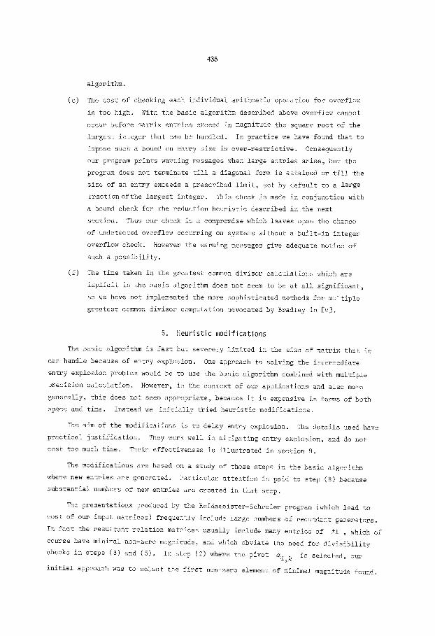
(e) The cost of checking each individual arithmetic operation for overflow

is too high. With the basic algorithm described above overflow cannot

occur before matrix entries exceed in magnitude the square root of the

largest integer that can be handled. In practice we have found that to

impose such a bound on entry size is over-restrictive. Consequently

our program prints warning messages when large entries arise, but the

program does not terminate till a diagonal form is attained or till the

size of an entry exceeds a prescribed limit, set by default to a large

fraction ofthe largest integer. This check is made in conjunction with

a bound check for the reduction heuristic described in the next

section. Thus our check is a compromise which leaves open the chance

of undetected overflow occurring on systems without a built-in integer

overflow check. However the warning messages give adequate notice of

such a possibility.

(f) The time taken in the greatest common divisor calculations which are

implicit in the basic algorithm does not seem to be at all significant,

so we have not implemented the more sophisticated methods for multiple

greatest common divisor computation advocated by Bradley in [4].

5. Heurist ic modifications

The basic algorithm is fast but severely limited in the size of matrix that it

can handle because of entry explosion. One approach to solving the intermediate

entry explosion problem would be to use the basic algorithm combined with multiple

precision calculation. However, in the context of our applications and also more

generally, this does not seem appropriate~ because it is expensive in terms of both

space and time. Instead we initially tried heuristic modifications.

The aim of the modifications is to delay entry explosion. The details used have

practical justification. They work well in mitigating entry explosion, and do not

cost too much time. Their effectiveness is illustrated in section 9.

The modifications are based on a study of those steps in the basic algorithm

where new entries are generated. Particular attention is paid to step (8) because

substantial numbers of new entries are created in that step.

The presentations produced by the Reidemeister-Sehreier program (which lead to

most of our input matrices) frequently include large numbers of redundant generators.

In fact the resultant relation matrices usually include many entries of ±i , which of

course have minimal non-zero magnitude, and which obviate the need for divisibility

checks in steps (3) and (5). In step (2) where the pivot a£, k is selected, our

initial approach was to select the first non-zero element of minimal magnitude found.

430

In particular as soon as a ±i was found, it was ahosen~ leading rapidly to step (8).

Clearly the size of the elements in the row including the chosen pivot with unit

magnitude has a fundamental effect on the size of the new entries created in step (8).

Our first modification takes this into account. If there is more than one entry with

magnitude i we select as pivot an entry in a row for which the sum of the absolute

values of the entries (which we call row sum) is "small". (In practice our program

has a parameter, under user control, which specifies what rates as a small row sum.

The first unit entry found with small row sum is selected as pivot~ and, if there is

none with small row sum, then a unit entry with minimal row sum is used. Alternative

measures merit consideration, for example~ the product of row and column sums.)

One effect of the preference given to row additions in the basic algorithm is

that, after a while, the rows in the matrix remaining under consideration begin to

resemble one another and large entries tend to gather in columns. This means that

rows can be improved by straightforward addition or subtraction, and it turns out that

this is worthwhile.

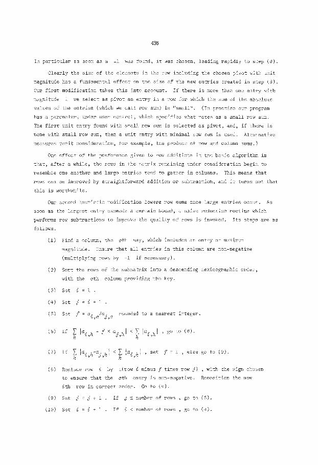
Our second heuristic modification lowers row sums once large entries occur. As

soon as the largest entry exceeds a certain bound, a naive reduction routine ~hich

performs row subtractions to improve the quality of rows is invoked. Its steps are as

follows.

(i) Find a column, the oth say, which includes an entry of maximum

magnitude. Ensure that all entries in this column are non-negative

(multiplying rows by -i if necessary).

(2) Sort the rows of the submatrix into a descending lexicographic order,

with the eth column providing the key.

(3) S e t i : i .

(4) Set j = { + 1 .

(5) Set f = a. /a. rounded to a nearest integer.

(6) If ~h lai'h - f x aj,hl < ~ lai,hl ~ go t o (8).

(7) If Z lai,h-aj,h I <~ h lai'hl ~ set f = 1 , else go to (9). h

(8) Replace row i by ±(row i minus f times row j) , with the sign chosen

to ensure that the cth entry is non-negative. Reposition the new

ith row in correct order. Go to (4).

(9) Set j : j + i . If j ~ number of rows ~ go to (5).

(i0) Set i : i + i . If i < number of rows ~ go to (4).

437

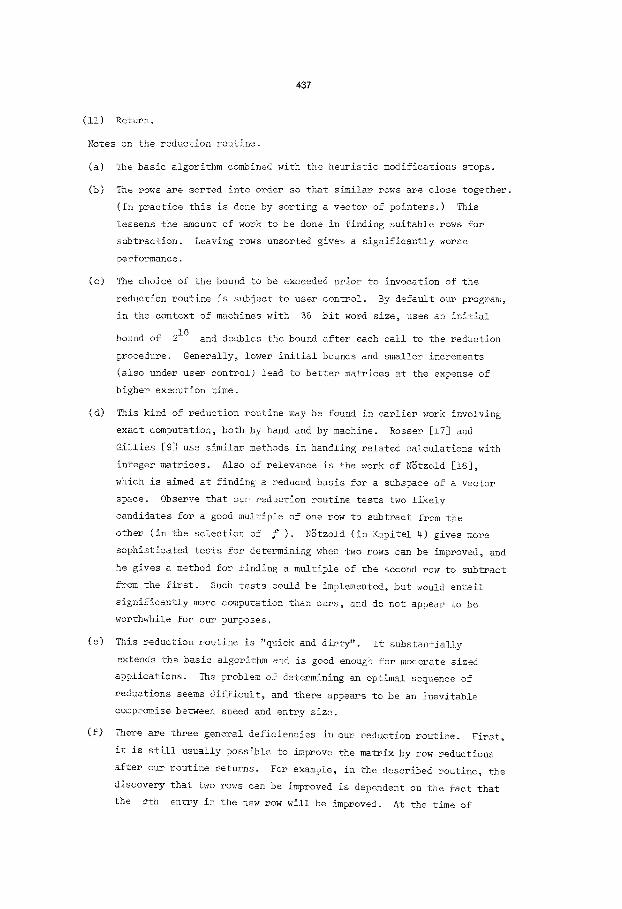
(ii) Return.

Notes on the reduction routine.

(a) The basic algorithm combined with the heuristic modifications stops.

(b) The rows are sorted into order so that similar rows are close together.

(In practice this is done by sorting a vector of pointers.) This

lessens the amount of work to be done in finding suitable rows for

subtraction. Leaving rows unsorted gives a significantly worse

performance.

(c) The choice of the bound to be exceeded prior to invocation of the

reduction routine is subject to user control. By default our program,

in the context of machines with 36 bit word size, uses an initial

bound of 210 and doubles the bound after each call to the reduction

procedure. Generally, lower initial bounds and smaller increments

(also under user control) lead to better matrices at the expense of

higher execution time.

(d) This kind of reduction routine may be found in earlier work involving

exact computation, both by hand and by machine. Rosser [17] and

Gillies [9] use similar methods in handling related calculations with

integer matrices. Also of relevance is the work of N~tzold [16],

which is aimed at finding a reduced basis for a subspace of a vector

space. Observe that our reduction routine tests two likely

candidates for a good multiple of one row to subtract from the

other (in the selection of f ). NStzold (in Kapitel 4) gives more

sophisticated tests for determining when two rows can be improved, and

he gives a method for finding a multiple of the second row to subtract

from the first. Such tests could be implemented, but would entail

significantly more computation than ours, and do not appear to be

worthwhile for our purposes.

(e) This reduction routine is "quick and dirty". IT substantially

extends the basic algorithm and is good enough for moderate sized

applications. The problem of determining an optimal sequence of

reductions seems difficult, and there appears to be an inevitable

compromise between speed and entry size.

(f) There are three general deficiencies in our reduction routine. First,

it is still usually possible to improve the matrix by row reductions

after our routine returns. For example, in the described routine, the

discovery that two rows can be improved is dependent on the fact that

the cth entry in the new row will be improved. At the time of

438

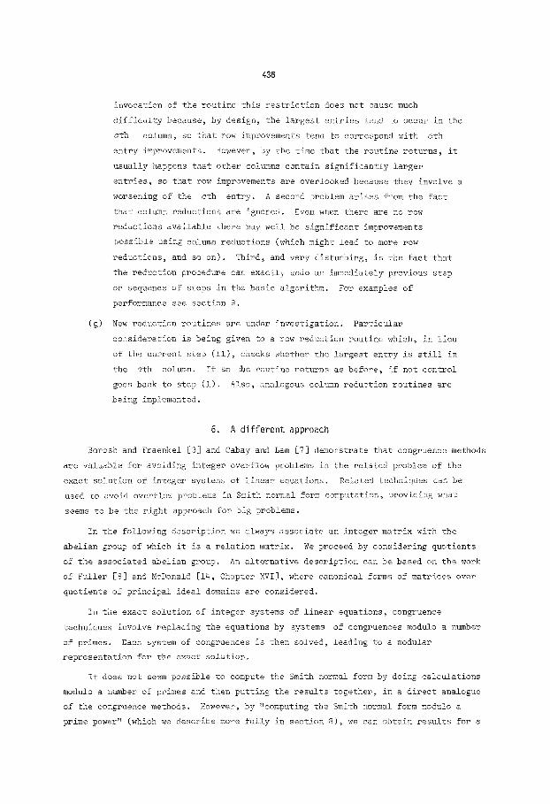
(g)

invocation of the routine this restriction does not cause much

difficulty because, by design, the largest entries tend to occur in the

cth column, so that row improvements tend to correspond with oth

entry improvements. However, by the time that the routine returns~ it

usually happens that other columns contain significantly larger

entries, so that row improvements are overlooked because they involve a

worsening of the cth entry. A second problem arises from the fact

that column reductions are ignored. Even when there are no row

reductions available there may well be significant improvements

possible using column reductions (which might lead to more row

reductions, and so on). Third, and very disturbing, is the fact that

the reduction procedure can exactly undo an immediately previous step

or sequence of steps in the basic algorithm. For examples of

performance see section 9.

New reduction routines are under investigation. Particular

consideration is being given to a row reduction routine which, in lieu

of the current step (ii), checks whether the largest entry is still in

the cth column. If so the routine returns as before, if not control

goes back to step (i). Also, analogous column reduction routines are

being implemented.

6. A different approach

Borosh and Fraenkel [3] and Cabay and Lam [7] demonstrate that congruence methods

are valuable for avoiding integer overflow problems in the related problem of the

exact solution of integer systems of linear equations. Related techniques can be

used to avoid overflow problems in Smith normal form computation, providing what

seems to be the right approach for big problems.

In the following description we always associate an integer matrix with the

abelian group of which it is a relation matrix. We proceed by considering quotients

of the associated abelian group. An alternative description can be based on the work

of Fuller [8] and McDonald [14, Chapter XVI], where canonical forms of matrices over

quotients of principal ideal domains are considered.

In the exact solution of integer systems of linear equations, congruence

techniques involve replacing the equations by systems of congruences modulo a number

of primes. Each system of congruences is then solved, leading to a modular

representation for the exact solution.

It does not seem possible to compute the Smith normal form by doing calculations

modulo a number of primes and then putting the results together, in a direct analogue

of the congruence methods. However, by "computing the Smith normal form modulo a

prime power" (which we describe more fully in section 8), we can obtain results far a

439

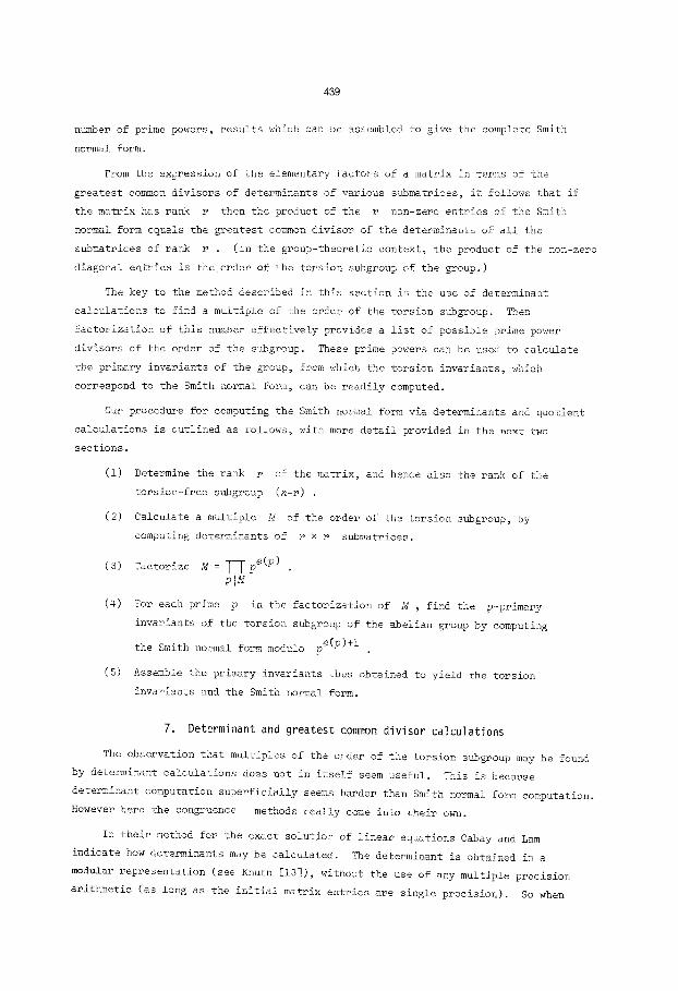
number of prime powers, results which can be assembled to give the complete Smith

norm~l form.

From the expression of the elementary factors of a matrix in terms of the

greatest common divisors of determinants of various submatrices, it follows that if

the matrix has rank r then the product of the r non-zero entries of the Smith

normal form equals the greatest common divisor of the determinants of all the

submatrices of rank r . (In the group-theoretic context, the product of the non-zero

diagonal entries is the order of the torsion subgroup of the group.)

The key to the method described in this section is the use of determinant

calculations to find a multiple of the order of the torsion subgroup. Then

faetorization of this number effectively provides a list of possible prime power

divisors of the order of the subgroup. These prime powers can be used to calculate

the primary invariants of the group, from ~nich the torsion invariants, which

correspond to the Smith normal form, can be readily computed.

Our procedure for computing the Smith normal form via determinants and quotient

calculations is outlined as follows, with more detail provided in the next two

sections.

(I) Determine the rank r of the matrix, and hence also the rank of the

torsion-free subgroup (n-r) .

(2) Calculate a multiple M of the order of the torsion subgroup, by

computing determinants of r × r submatriees.

(3) Factorize M = p~Mp e(p)

(4) For each prime p in the factorization of M , find the p-primary

invariants of the torsion subgroup of the abelian group by computing

the Smith normal form modulo pe(p)+l .

(5) Assemble the primary invariants thus obtained to yield the torsion

invariants and the Smith normal form.

7. Determinant and greatest common divisor calculations

The observation that multiples of the order of the torsion subgroup may be found

by determinant calculations does not in itself seem useful. This is because

determinant computation superficially seemsharder than Smith normal form computation.

However here the congruence methods really come into ~beir own.

In their method for the exact solution of linear equations Cabay and Lam

indicate how determinants may be calculated. ~e determinant is obtained in a

modular representation (see Knuth [13]), without the use of any multiple precision

arithmetic (as long as the initial matrix entries are single precision). So when

440

integer overflow threatens elimination methods we resort to determinant calculation~

using the techniques of Cabay and Lam, combined with quotient calaulations~

Some comments on implementation are appropriate. The first problem is the

determination of the rank r of the matrix over the integers. By default our

program "guesses" r by computing the rank modulo a large prime. The guess is

correct unless the prime divides the order of the torsion subgroup~ and the

likelihood of this happening is very low.

The rank may be determined exactly, at the expense of extra time. The Hadamard

hound for determinants is used by Cabay and Lam to provide a stopping criterion

for their algorithm. An analogue may be used for rank determination. If we have an

m × n matrix A = Iai,jl , then certainly any subdeterminant of A is bounded above

in magnitude by I I ~ ai,jl We can choose a number of primes whose product i:l Sl

exceeds this hound and ensure correct rank determination by computing the rank modulo

each of these primes. Since the product of the primes necessarily exceeds each

subdeter~inant~ at least one of the primes does not divide any particular

subdeterminant~ and thus at least one of the primes does not divide the order of the

torsion subgroup. The maximum rank obtained this way is the correct rank of A over

the integers.

In the process of computing the rank r , we simultaneously find an r x r

submatrix which is nonsingular, whose determinant we calculate. Once we have one

non-zero determinant of an r x r suhmatrix we have a multiple of the order of the

torsion subgroup. There are two difficulties: first~ in cases where integer

overflow troubles elimination methods, the determinant is usually a very large number

in modular representation; second, the determinant of just one r x r submatrix

often provides a multiple which is orders of magnitude larger than the order of the

torsion subgroup (see section 9 for examples).

Because of the size of the determinants that arise we may be forced to resort to

multiple precision calculation at this stage of the process. If necessary, we use

the t£n package of Brent [5] to calculate fixed radix representations of the

determinants. (We need to convert to fixed radix representation for our determinants

so that we can readily perform our subsequent calculations. Good methods for

division with numbers in modular representation are not known~ and division is the

basis of greatest common divisor calculations and faatorization, which we do next.)

While one determinant may provide a large multiple of the order of the torsion

subgroup, the greatest common divisor of a small number of determinants of distinct

r x r submatrices generally provides a reasonable multiple (again, see section 9).

So we often compute a few determinants and their greatest common divisor (very easily

done with MP , if necessary) to obtain our multiple of the order of the torsion

441

subgroup.

Our routine method of selection of a number of nonsingular r x r submatrices is

such that the calculation of a number of determinants takes very little extra time

over that taken to compute one determinant. Having found one nonsingular ~ x

submatrix we simply replace the last row (column in the case of matrices with m < n )

of the initial r × ~ submatrix by a new row (column) which is independent of the

previous r - i rows (columns), so that most of the computation for each of the

number of determinants is done simultaneously.

Cabay and Lam have two different stopping criteria for their algorithm for the

exact solution of linear equations. The first criterion, based on the Hadamard bound

for matrix determinants, ensures correct determinant calculation and is incorporated

in our program. Their other criterion, even though it does not guarantee that the

determinant has been fully calculated, is also of value. This criterion, called the

recursive test, is more fully described in Cabay [6] and Bareiss [i].

The kinds of matrices that we encounter are such that each row sum is less than

the smallest prime which is used as a modulus in the determinant calculation. Tt

follows from the recursive test that, when the first zero mixed radix coefficient for

the determinant is found, the mixed radix coefficients must already represent a

divisor of the determinant. We use this as an early stopping criterion in our

determinant calculation routine, in spite of the fact that there is no guarantee that

the nu,,~er thus represented is not a proper divisor of the determinant. The criterion

substantially reduces determinant calculation time with only little risk of producing

incorrect results. Except in the case of specially constructed examples the early

stopping criterion has never led to incorrect results in practice, and we normally use

it for preliminary calculations in order to speed things up. When we require absolute

assurance of our determinant calculations we use the original criterion based on the

Hadamard bound.

8. ~4odular calculations

Having found a multiple M of the order of the torsion subgroup, we first find

its prime factorization, M : Epe(P) It would be wrong to pass blithely over this

step, because it is well known that prime factorization of large numbers is difficult

(see Knuth [13]). However, for abelian groups whose presentations have arisen

"naturally" we have found that this is not a problem. Their torsion subgroups

generally seem to have orders involving only a small number of low primes, and, in

practice, the multiple produced by our calculations has always been good enough for

factorization to pose no substantial difficulties.

For each prime p in the factorization of M , we compute the p-power primary

invariants of g by considering the maximal quotient H of g which has exponent

442

d p The choice of d is made so that the largest p-primary invariant of ~ is a

d proper divisor of p

Consider the p-primary invariants of G ~ {pe(p,l) e(p,2) pe(p,k)}

Then H has primary (and torsion) invariants

{pe(p,l), pC(p,2) ..... pe(p,k) pd ..... pd} ,

d where each p corresponds to a torsion-free factor in a decomposition of G , and

each other invariant corresponds to a cycle in a primary decomposition of G with

that order.

Consider the abelian group H of exponent pd defined on n generators Yi by

the m relations ~ ai~jY i = 0 , and its associated relation matrix A . It is easy

to see that the following transformations of the relations leave the group unchanged:

• _ pd (i) replacement of a ,j by ai, j + ;

(2) multiplication of any relation by any unit of the ring of integers

modulo pd .

d We now define Smith normal form calculation modulo a prime power p

corresponding to the above transformations~ so that the process converts the relation

matrix A to a canonical form which provides the torsion invariants for H . An

d algorithm for Smith normal form computation modulo a prime power p is the same as

the basic algorithm of section 2, with the following exceptions. First, at all stages

in the process, matrix entries are replaced by their residues modulo pd . Second,

step (2) is replaced by:

(2 4 ) Find a non-zero matrix element, ai, k say, whose greatest common

d divisor with p is minimal. Multiply row i by a unit, u say,

which is such that u x ai, k is a power of p .

~nivd, it follows that steps (3) to (6) are not necessary because, after multiplication

by u ~ ai, k divides all entries in its row and column. The other steps are

d unchanged. Provided p is not too large, this algorithm does not suffer from

integer overflow problems.

The algorithm and canonical form are essentially the same as those of Fuller.

The diagonal entries of the form provide the torsion invariants of H ~ and thus the

p-primary invariants of G .

Since from the factorization of M , we have a list of all possible primes

443

involved in the torsion invarian~s of G , we can reconstruct the torsion invariants

of G fully. Notice that for d we routinely choose e(p) ÷ I , which must be large

d enough for every p-primary invariant of G to be a proper divisor of p However

smaller values may suffice, and it is easily possible to check if a smaller value does

suffice, because the ranks of the torsion and torsion-free subgroup are known. A

d Smith normal form calculation modulo p yields the p-primary invariants of G

if there are precisely r non-zero diagonal entries. Otherwise G has p-primary

d invariants which are multiples of p

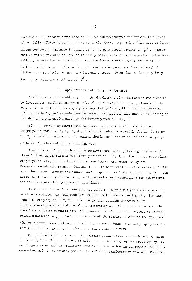
9. Applications and program performance

The initial stimulus which sparked the development of these methods was a desire

to investigate the Fibonacci group E(2, 9) by a study of abelian quotients of its

subgroups. Results of this inquiry are reported by Havas, Richardson and Sterling

[12], where background material may be found. We start off this section by looking at

the abelian decomposition phase of the investigation of F(2, 9).

F(2, 9) may be presented with two generators and two relations, and has

subgroups of index 2, 4, 8, 192 3S, 76 and 152 , which are readily found. We denote

by H. a relation matrix for the maximal abelian quotient of one of these subgroups

of index i ~ obtained in the following way.

Presentations for the subgroups themselves were found by finding subgroups of

these indices in the maximal nilpotent quotient of F(2, 9) . Then the corresponding

subgroups of F(2, 9) itself, with the same index, were presented by the

Reidemeister-Schreier program, denoted RS . The naive abelianization methods of RS

were adequate to identify the maximal abelian quotients of subgroups of F(2, 9) with

index 2, 4 and 8 , but did net provide recognizable presentations for the maximal

abelian quotients of subgroups of higher index.

In this section we first tabulate the performance of our algorithms on relation

matrices associated with subgroups of F(2~ 9) with index exceeding 8 . For each

index i subgroup of F(9, 9) , the presentation produced directly by the

Reidemeister-Schreier method has i + i generators and 2i relations, so that the

associated relation matrices have 2i rows and i + i columns. Because of initial

problems handling HI52 , caused by the size of the matrix, we went to the trouble of

finding a better presentation for the (unique normal) index 152 subgroup by working

down a chain of subgroups, in order to obtain a smaller matrix.

RS produced a 3 generator~ 4 relation presentation for a subgroup of index

2 in F(2, 9) . Then a subgroup of index 4 in this subgroup was presented by RS

on 9 generators and 16 relations, and this presentation was replaced by one on 4

generators and 9 relations, produced by a Tietze transformation program. From this

444

presentation RS produced a 58 generator~ 171, relation presentation for a

subgroup of index 19 . We denote by H2,4,19 a relation matrix for the maximal

abelian quotient of this index 152 subgroup of F(2, 9) obtained from this

presentation. Finally we denote by HI90 a relation matrix for the maximal abelian

quotient of a subgroup of F(2, 9) with index 190 ~ which was found as a consequence

of calculations described in [123,

All results in this section are based on computer runs. We used a DEC KAI0, with

memory cycle time of 950 nanoseconds. Times quoted are in CPU seconds. Despite

some variability due to the nature of DEC-10 timing methods, they provide a reasonable

guide to relative performance. This machine was ideal for our purposes because it has

a hardware integer overflow check which is utilized by the FORTRAN operating system.

Integers in FORTRAN on the DEC-10 are restricted to the range -(235-i] to 285 - i .

Performance on Matrices Derived from F(2, 9)

HIg

Bows 38

Ool~rr~S 20

Torsion invariants 2,2

Eliminations ~sic) 13

Time (basic) 1.3

Eliminations 2O

(mod{ ~ed)

Reductions i

Time (modified) I. 4

H38 I H76

76 152

39 77

4 2

27 51

q,9 22.1

39 75

4 ii

12.5 251

Firs# determinant 19752 613568 6789296

G.c,d. 8 32 65536 = 215

Primes (rec./Had.) 2/2 3/4 3/7

Time (Had., i ~t.) 2.4 13.3 80

Time (rec., i ~t.) 2.4 ll.l 45

Time (Had., d.) 5.2 17,5 88

Time (rec., g. .d.) 5.2 12.6 51

Time (modular) 1.4 6.2 34.5

H152

304

153

eighteen

104

108

124

14

1457

22.72.52o

22.72.520

5/13

724

346

937

538

192

5TS

H2,4,19

171

58

eighteen 5's

21

20 .i

48

19

492

23.32.519

3.519

4/8

81

46

90

53

45

HI90

380

191

4

149

133

146

15

2674

~ I x i017

256

5/15

1519

627

1568

643

336

NOTES. (a) The top section of the table describes the nature of the matrices

involved. In only one case, H2,4,19 , does an initial matrix include entries which

exceed i in magnitude, H2,4,19 has entries with magnitude up to 3 . The torsion

445

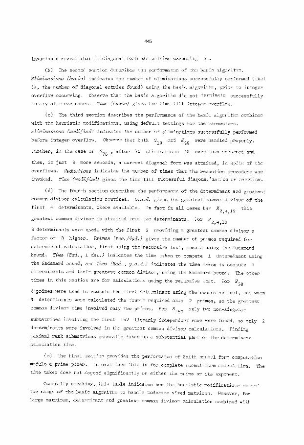
invariants reveal that no diagonal form has entries exceeding 5 °

(b) The second section describes the nerformance of the basic algorithm.

Eliminations (basic) indicates the n~m~er of eliminations successfully performed (that

is, the number of diagonal entries found) using the basic algorithm, prior to integer

overflow occurring. Observe that the basic algorithm did not terminate successfully

in any of these cases. Time (basic) gives the time till integer overflow.

(c) The third section describes the performance of the basic algorithm combined

with the heuristic modifications, using default settings for the parameters.

Eliminations (modified) indicates the number of eliminations successfully performed

before integer overflow. Observe that both HI9 and H38 were handled properly.

Further, in the case of H76 , after 75 eliminations i0 overflows occurred and

then, in just 3 more seconds, a correct diagonal form was attained~ in spite of the

overflows. Reductions indicates the number of times that the reduction procedure was

invoked. Time (modified) gives the time till successful diagonalization or overflow.

(d) The fourth section describes the performance of the determinant and greatest

common divisor calculation routines. G.c.d. gives the greatest common divisor of the

first ~ determinants, where available. In fact in all cases bar H2~4~19 this

greatest common divisor is attained from two determinants. For H2,4,19

3 determinants were used~ with the first 2 providing a greatest com~mon divisor a

factor of 3 higher. Primes (rec./H~d.) gives the number of primes required for

determinant calculation, first using the recursive test, second using the Hadamard

bound. Time (Had., i dot.) indicates the time taken to compute I determinant using

the Hadamard bound, and Time CHad., g.c.d.) indicates the time taken to compute 4

determinants and their greatest common divisor, using the Hadamard bound. The other

times in this section are for calculations using the recursive test. For H38

3 primes were used to compute the first determinant using the recursive test, but when

4 determinants were calculated the fourth required only 2 primes, so the greatest

common divisor time involved only two primes. For HI52 only two non-singular

submatrices involving the first 152 linearly independent rows were found, so only 2

determinants were involved in the greatest common divisor calculations. Finding

maximal rank submatrices generally takes up a substantial part of the determinant

calculation time.

(e) The final section provides the performance of Smith normal form computation

modulo a prime power. In each case this is for complete normal form calculation. The

time taken does not depend significantly on either the prime or its exponent.

Generally speaking, ~his table indicates how the heuristic modifications extend

the range of the basic algorithm to handle moderate sized matrices. However, for

large matrices, determinant and greatest common divisor calculation combined with

446

modular computation is the winning approach.

The time cost of the heuristic modifications is reasonable for moderate sized

matrices, but grows inordinately for large matrices. Worse still, as is evidenced by

]190 ' even with an enormous amount of time, the heuristic modifications occasionally

hindered rather than helped the computation.

Note specifically that, in modular computation for index 152 subgroups of

F(2, 9) , ou_~ default exponent for 5 ~ namely 20 or 21 , was not suitable for use

because 520 is too large. However computation modulo 52 was adequate to compute

the normal form.

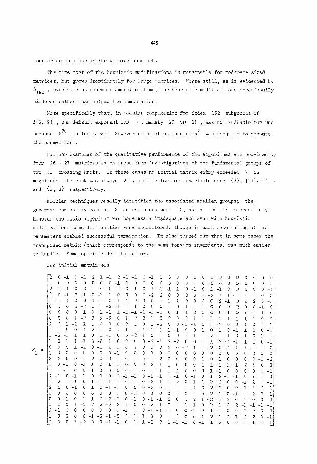
Further examples of the qualitative performance of the algorithms are provided by

four 26 x 27 matrices which arose from investigations of the fundamental groups of

two ii crossing knots. In these cases no initial matrix entry exceeded 7 in

magnitude, the rank was always 25 , and the torsion invariants were {3}, {14}, {2} ,

and {3, 3} respectively.

Modular techniques readily identified the associated ahelian groups; the

greatest common divisors of 3 determinants were 15, 56, 6 and 18 respectively.

However the basic algorithm was hopelessly inadequate and even with heuristic

modifications some difficulties were encountered, though in each case tuning of the

parameters enabled successful termination. It also turned out that in some cases the

transposed matrix (which corresponds to the same torsion invariants) was much easier

to handle. Some specific details follow.

One initial

Ii 0 -i 0

2 0 0 0 I -i 0 0 -I 2

-1 1 0 00 2

0 0 0 0 0 0 0 ! 2 2 1 - 2 1 1 0 0 i -2 -i 1 1 0 i 1 0 0 0 1 R :

1 1 0 0 0 3 2 0 0 i 0 -i 0 1 1 -I 0 2 -i 0 -i 12 i -i 2 i 0 -I 0 0 0 0 00 -i 0 1 1 0 1 2 -i 0 0 1 0 0 0 2 0 0 1

matrix was

- 1 2 1 - 1 9 - 1 - 1 0 - 1 1 0 0 0 0 0 0 0 0 0 0 0 0 1 0 0 0 0 - i 0 0 0 0 0 0 0 0 1 0 0 0 0 0 0 0 0 ~ 0 1 0 0 0 0 1 0 1 -i -i -I 0 -I 01 - 1 0 0 0 0 0 -

- 1 0 - 1 1 0 0 0 0 - 2 2 0 0 0 0 ] - 2 1 1 - 1 1 - 1 0 0 0 - i 0 - 1 l 0 0 0 1 1 - 1 0 0 0 0 2 - 1 0 ~ 2 0 -

-211 -2 -i I i 0 0 0 -i 01 -i i 0 0 0 2 0 0 -1 1 0 1 -I i -i -i -i -I -i 0 1 1 0 0 0 0 -i 0 -l -I 1

-202 - 2 0 1 2 0 1 0 2 0 -21 ! -i -i -i 11 -i 0 ~ 1 1 0 0 0 0 1 0 1 -200 -1 -I 01 -200 -101 -2

-12 -i 02 -i -i -I -i -11 - 1 0 0 1 0 1 0 - 1 1 0 0 -I 1 0 1 -100 -2 -i 0 1 0 0 1 1 1 -21 -i 0 1 0 1 1

-i 0 - 3 1 0 0 0 0 -2 -i 2 - 2 0 0 1 1 2 -i -i 1 1 0 -i -20 - 1 1 1 0 1 0 0 0 2 0 -211 -201 -I 1 -I 10 0 0 0 0 - i 0 0 0 0 0 0 0 0 0 0 0 0 0 0 0 0 0 0

- 2 2 0 0 1 0 1 0 - 1 - 2 0 0 0 0 1 0 1 0 0 0 0 - 1 - 2 -i 1 0 1 1 0 0 0 -2 -i 1 0 0 0 1 -i 1 -i -i 2 -100 0 1 0 0 0 0 1 0 1 -i -i - 1 0 0 0 1 - 1 0 0 0 0 0 -i 1 0 0 0 0 -i -i 0 -i -I 0 -i 0 -i 0 1 2 -i -i 01 -i 0 0 i -i 1 1 0 1 0 -2 -I 1 2 0 -i ! 0 2 0 0 -110 -2 0 1 0 - 1 - 1 0 0 0 - 2 0 - 1 - 1 1 - 1 0 2 2 0 0 - 1 1 - 2 - 1 0 0 0 0 1 0 - 1 0 0 0 0 - 2 0 1 0 -2 -i 0 -i 2 -20 li

-112 -200 -i 0 -i -i 2 0 0 2 i -22 - 2 0 2 0 0 0 1 -222 -22 -i 00 -2 -i 0 1 1 - 1 0 0 1 0 2 -i -I -i -1 0 0 0 0 1 -i 10 -i -i -i 00 - 3 0 1 1 0 0 -i 0 0 0 0 -1 -2 -i - 3 2 1 1 0 2 I -200 -i 2 1 0 -I -220 -I

- 2 0 0 - 1 - 1 0 1 1 - 2 2 1 - 1 - i 0 - 1 1 2 0 0 - 1 t - 1 - ~

4 4 7

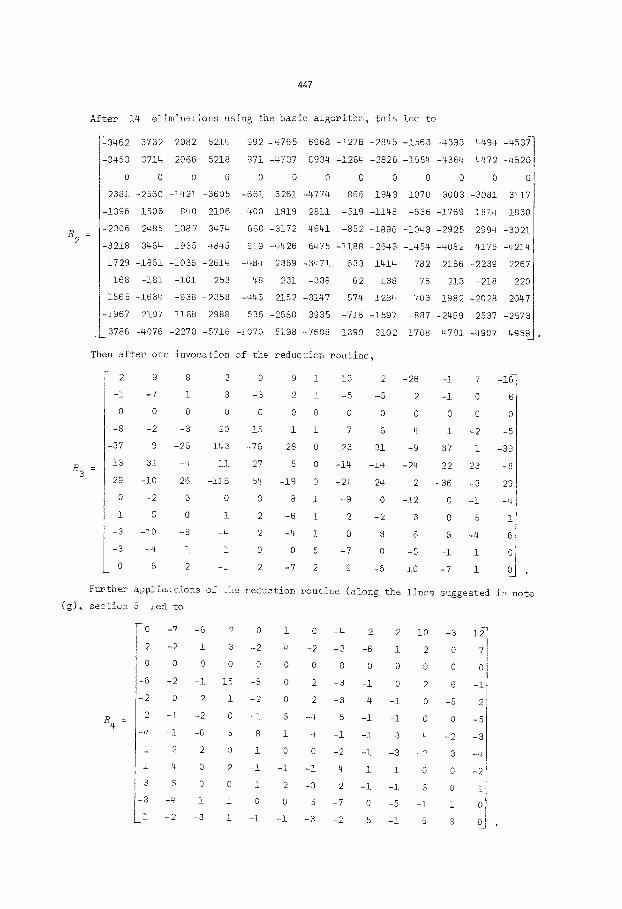
R 2

/{3 =

After ].4 eliminations using the basia algorithm, this

~3462 3732 2082 5214 992 -4765 6968 -1276 -2845

-3453 3714 2066 5218

0 0 0 0

2381 -2560 -1421 -3605

-1396 1506 840 2106

-2306 2485 1387 3474

-3218 3464 1935 4845

1729 -1861 -1036 -2614

168 -181 -i01 -253

1565 -1684 -938 -2358

-1967 2107 1168 2988

3786 -4076 -2270 -5716

Then after one invocation

2 9 8 3

-i -7 i 3

0 0 0 0

-8 -2 -3 20

-37 9 -25 143

13 31 -4 !i

29 -i0 26 -i16

0 - 2 3 0

i 5 0 I

-3 - 10 -8 -4

-3 -4 i i

0 6 2 -i

led to

-!563 -4393 4494 -453~

971 -4737 6934 -1264 -2826 -1554 -4364 4472 -4820

0 0 0 0 0 0 0 0 0

-661 3261 -4774 866 1943 1070 3003 -3081 3117

400 -1919 2811 -519 -1148 -636 -1769 1814 -1830

660 -3172 4641 -852 -1896 -1048 -2928 2994 -3021

919 -4426 6475 -1188 -2643 -1454 -4082 4175 -4214

-484 2369 -3471 633 1414 782 2186 -2239 2267

-48 231 -338 62 138 76 213 -218 220

-446 2152 -3147 574 1284 703 1982 -2028 2047

536 -2680 3935 -716 -1597 -887 -2469 2537 -2573

-1070 5198 -7608 1390 3102 1708 4791 -4907 4959--

of the reduction routine,

0 9 i -13 2 -26 -i 7 -16

-3 2 I -5 -5 2 -i 0 6

0 0 0 0 0 0 0 0 0

-!5 i i 7 6 4 I -2 -5

-76 28 0 23 31 -9 37 I -39

27 5 0 -14 -!4 -24 22 23 -8

54 -19 0 -21 -24 2 -36 -3 29

0 8 i -9 0 -12 0 -I -4

2 -6 i 2 -2 3 0 5 i

2 -4 1 0 8 6 6 -4 6

0 0 5 -7 0 -5 -i 1 0

2 -7 2 9 -6 i0 -7 i 0

Further applications of the reduction

(g), section 5 led to

-0 -7

2 -2

0 0

-6 -2

-2 0

2 -i B 4 =

-4 -i

i 2

i 4

3 5

-3 -4

LI -2

routine (along the lines suggested in note

-6 2 0 i 0 -4 2 2 i0 -3 12

i 3 -2 4 -2 -3 -6 i 2 0 7

0 0 0 0 0 0 0 0 0 0 0

-i 15 -8 0 2 -3 -i 0 2 6 -i

2 1 - 2 0 2 -3 4 -1 0 -5 2 i

-2 0 -i 8 -4 5 -i -i 0 0 -5 i

-6 5 8 i 4 -i -i 3 4 -2 -3

2 0 1 0 0 -2 -1 -3 - 2 3 -4

0 2 -i -i -i 4 i I 0 0 -2

0 0 1 2 -3 2 -i -i 3 0 i

i i 0 0 5 -7 0 -5 -i i 0

-3 i -I -i -3 -2 5 -i 5 3 0

448

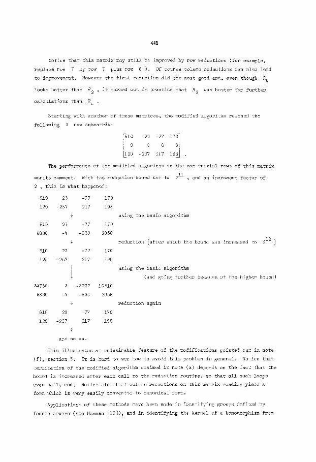
Notice that this matrix may still be improved by row reductions (for example,

replace row 7 by row 7 plus row 8 ). Of course column reductions san also lead

to improvement. However the first reduction did the most good and, even though R 4

looks better than R 3 , it turned out in practice that R 3 was better for further

calculations than R 4 .

Starting with another of these matrices, the modified algorithm reached the

following 3 row submatrix:

770 ~20 -257 217 198~ .

The performance of the modified algorithm on the non-trivial rows of this matrix

merits comment. With the reduction bound set to 211 , and an increment factor of

2 , this is what happened:

610 23 -77 170

120 -257 217 198

+ using the basic algorithm

610 23 -77 170

6830 -4 -630 2068

% reduction (after which the bound was increased to 212 ]

610 23 -77 170

120 -257 217 198

I using the basic algorithm

(and going further because of the higher bound)

34760 3 -3227 10510

6830 -4 -630 2068

+ reduction again

610 23 -77 170

120 -257 217 198

+

and so on.

This illustrates an undesirable feat<~e of the modifications pointed out in note

(f), section 5. It is hard to see how to avoid this problem in general. Notice that

termination of the modified algorithm claimed in note (a) depends on the fact that the

bound is increased after each call to the reduction routine, so that all such loops

eventually end. Notice also that column reductions on this matrix readily yield a

form which is very easily converted to canonical form.

Applications of these methods have been made in identifying groups defined by

fourth powers (see Newman [15]), and in identifying the kernel of a homomorphism from

449

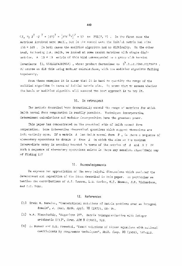
<X, Y; X 7 =Y 7 = (Xy)7 : [XYX-Iy]2 = i> to PSL(2, 7) . In the first case the

matrices involved were small, but in the second case the initial matrix had size

156 × 169 . In both cases the modified algorithm had no difficulty. On the other

hand, following D.A. Smith, we looked at some random matrices with single digit

entries. A 13 × 13 matrix of this kind corresponded to a group with torsion

invariants {2, 50315164282968} , whose product factorizes to 24.3.13.7993.20175973 .

Of course we did this using modular calculations, with the modified algorithm failing

hopelessly.

From these examples it is clear that it is hard to quantify the range of the

modified algorithm in terms of initial matrix size. It seems that to assess whether

the basic or modified algorithm will succeed the best approach is to try it.

I0. In retrospect

The methods described here dramatically extend the range of matrices for which

Smith normal form computation is readily possible. Techniques incorporating

determinant calculations and modular decomposition have the greatest power.

This paper has concentrated on the practical side of Smith normal form

computation. Some interesting theoretical questions which suggest themselves are

left entirely open. If a matrix A has Smith normal form B , is there a sequence of

elementary operations to obtain B from A in which the size of the maximum

intermediate entry is sensibly bounded in terms of the entries of A and B ? If

such a sequence of elementary operations exists is there any sensible algorithmic way

of finding it?

11. Acknowledgements

We express our appreciation of the many helpful discussions which assisted the

development and exposition of the ideas described in this paper. In particular we

mention the contributions of J.J. Cannon~ L.G. Kov~cs, M.F. Newman~ J.S. Richardson,

and C.C. Sims.

12, References

[I] Erwin H. Bareiss, "Computational solutions of matrix problems over an integral

domain", J. Inst. Math. Appl. ]0 (1972), 68-104.

[2] W.A. Blankinship, "Algoritb~m 287. Matrix triangularization with integer

arithmetic [FI]", Cow. ACM 9 (1986), 513.

[3] I. Borosh and A.S. Fraenkel, "Exact solutions of linear equations with rational

coefficients by congruence techniques", Math. Comp. 20 (1966), 107-112.

450

[4] Gordon H. Bradley, ~fA!gorithms for Hermite and Smith normal matrices and linear

Diophantine equations", Math. Comp. 25 (1971)~ 897-907.

[5] Richard P. Brent, "Algorithm 524. MP, a Fortran multiple-precislon arithmetic

package [AI]", ACM Trans. Math. Software 4 (1978)~ 71-81.

[6] Stanley Cabay, '~Exact solution of linear equations ~', Second Symposium on

Symbolic and Algebraic Manipulation, 392-398 (Proc. Ssmlpos. held Los

Angeles, 1971. Association for Computing Machinery~ New York, 1971).

[7] S. Cabay and T.P. Lam, "Congruence techniques for the exact solution of integer

systems of linear equations", ACM Trans. Math. Software 3 (1977), 386-397.

[8] L.E. Fuller, "A canonical set of matrices over a principal ideal ring modulo

m ", Canad. J. Math. 7 (1955), 54-59.

[9] D.B. Gillies, "The exact calculation of the characteristic polynomial of a

matrix", Information Processing (Proc. Internat. Conf. Information

Processing~ Paris, ].959, 62-66. UNESCO, Paris; 01denbourg~ Munchen;

9utterworths, London; 1960).

[i0] B. Hartley and T.O. Mawkes, Rings, modules and li~ea~ algebra (Chapman and

Hall~ London, Colchester~ 1970).

[11] George Havas, "A Reidemeister-Sehreier program", Proc. Second Internat. Conf.

Theory of Groups, Australian National University, Canberra, 1973~ 947-356

(Lecture Notes in Mathematics, 372. Springer-Verlag, Berlin, Heidelberg,

New York~ 1974).

[12] George Havas, J.S. Richardson and Leon S. Sterling~ "The last of the

Fibonacci groups"~ Proc. Roy. Soc. Edinburgh (to appear).

[]_3] Donald E. Knuth, The Art of Computer Progra~rming, Volume 2: Seminumerical

Algorithms (Addison-Wesley, Reading, Menlo Park, London, Don Hills, 1969).

[14] Bernard R. McDonald, Finite rings with identity (Marcel Dekker, New York, !974).

[15] M.F. Newman~ "A computer aided study of a group defined by fourth powers", Bull.

Austral. Math. Soc. ]4 (1976), 293-297.

[16] Ourgen N~tzold, "Uber reduzierte Gitterbasen und khre mogliehe Bedeutung fur die

numerische Behandlung linearer Gleichungss~teme'~, Dissertation,

Rheiniseh-Westfalsiehe Teahnisehe Hochschule, Aachen, 1976.

[17] d. Barkley Rosser, "A method of computing exact inverses of matrices with

integer coefficients", J. Ben. Nat. Bureau Standards 49 (1952)~ 349-358.

[18] Charles C. Sims~ "The influence of computers on algebras", Proc. Symp. Appl.

~th. 20 (!974), 13-30.

[19] David A. Smith, "A basis algorithm for finitely generated abe!ian groups", Math.

Algorithms ] (1966), 13-26.

451

[20] H.J.S. Smith, "On systems of linear indeterminate equations and congruences",

Philos. Trans. Royal Soc. London c]i (1861), 293-326. See also: The

Collected Mathematical Papers of Henry John Stephen Smith, Volume !,

367-409 (Chelsea, Bronx, New York~ 1965).