Infectious disease dynamics: a statistical perspective ...dept.stat.lsa.umich.edu/~ionides/talks/idd.pdf · Ed Ionides Infectious disease dynamics: ... Infectious disease dynamics:

Ed Ionides Infectious disease dynamics: a statistical perspective 1

Infectious disease dynamics: a statistical perspective

Epidemiology of Infectious Diseases Seminar

Harvard University

May 11, 2009

Ed Ionides

The University of Michigan, Department of Statistics


Collaborators

Anindya Bhadra (University of Michigan, Statistics)

Menno Bouma (London School of Hygiene and Tropical Medicine)

Carles Breto (Universidad Carlos III de Madrid, Statistics)

Daihai He (McMaster University, Mathematics & Statistics)

Aaron King (Univ. of Michigan, Ecology & Evolutionary Biology)

Karina Laneri (Univ. of Michigan, Ecology & Evolutionary Biology)

Mercedes Pascual (Univ. of Michigan, Ecology & Evolutionary Biology)


Infectious disease transmission: the public health challenge

Why do we seek to quantify and understand disease dynamics?

• Prevention and control of emerging infectious diseases (SARS,

HIV/AIDS, H5N1 “bird flu” influenza, H1N1 “swine flu” influenza)

• Understanding the development and spread of drug resistant strains

(malaria, tuberculosis, MRSA)


Disease dynamics: epidemiology or ecology, or both?

• Environmental host/pathogen dynamics are close to predator/prey

relationships which are a central topic of ecology.

• Analysis of diseases as ecosystems complements more traditional

epidemiology (risk factors etc).

• Ecologists typically seek to avoid extinctions, whereas epidemiologists

typically seek the reverse.


Infectious disease transmission: the statistical challenge

• Time series data of sufficient quantity and quality to support

investigations of disease dynamics are increasingly available.

• Statistical methods are required for partially observed, nonsta-

tionary, nonlinear, vector-valued stochastic dynamic systems.


Population models are typically partially observed Markov

processes (alias: state space models)

xt is an unobserved vector valued stochastic process (discrete or

continuous time).

– It is assumed to be Markovian, i.e., the past and future evolution of

the system are independent given its current state.

– This is reasonable if all important dynamic processes are modeled

as part of the system.

yt is a vector of the available observations (discrete time). These are

assumed to be conditionally independent given xt (a standard

measurement model, which can be relaxed).

θ is a vector of unknown parameters.


Plug-and-play inference for partially observed Markov

processes

• Statistical methods for pomps are plug-and-play if they require

simulation from the dynamic model but not explicit likelihood ratios.

• Bayesian plug-and-play:

1. Artificial parameter evolution (Liu and West, 2001)

2. Approximate Bayesian computation (“sequential Monte Carlo

without likelihoods,” Sisson et al, PNAS, 2007)

• Non-Bayesian plug-and-play:

3. Simulation-based prediction rules (Kendall et al, Ecology, 1999)

4. Maximum likelihood via iterated filtering (Ionides et al, PNAS, 2006)

Plug-and-play is a VERY USEFUL PROPERTY for investigating

scientific models.


Plug-and-play in other settings

• Optimization. Methods requiring only evaluation of the objective

function to be optimized are sometimes called gradient-free. This is

the same concept as plug-and-play: the code to evaluate the objective

function can be plugged into the optimizer.

• Complex systems. Methods to study the behavior of large simulation

models that only employ the underlying code as a “black box” to

generate simulations have been called equation-free (Kevrekidis

et al., 2003, 2004).

• This is the same concept as plug-and-play, but we prefer our label!

• A typical goal is to determine the relationship between macroscopic

phenomena (e.g. phase transitions) and microscopic properties (e.g.

molecular interactions).


The cost of plug-and-play

• Approximate Bayesian methods and simulated moment methods lead

to a loss of statistical efficiency.

• In contrast, iterated filtering enables (almost) exact likelihood-based

inference.

• Improvements in numerical efficiency may be possible when analytic

properties are available (at the expense of plug-and-play). But many

interesting dynamic models are analytically intractable—for example, it

is standard to investigate systems of ordinary differential equations

numerically.


Summary of plug-and-play inference via iterated filtering

• Filtering is the extensively-studied problem of calculating the

conditional distribution of the unobserved state vector xt given the

observations up to that time, y1, y2, . . . , yt.

• Iterated filtering is a recently developed algorithm which uses a

sequence of solutions to the filtering problem to maximize the

likelihood function over unknown model parameters.

(Ionides, Breto & King. PNAS, 2006)

• If the filter is plug-and-play (e.g. using standard sequential

Monte Carlo methods) this is inherited by iterated filtering.


Key idea of iterated filtering

• Bayesian inference for time-varying parameters becomes a solveable

filtering problem. Set θ = θt to be a random walk with

E[θt|θt−1] = θt−1 Var(θt|θt−1) = σ2

• The limit σ → 0 can be used to maximize the likelihood for fixed

parameters.


Theorem 1. (Ionides, Breto & King, PNAS, 2006)

Suppose θ0, C and y1:T are fixed and define

θt = θt(σ) = E[θt|y1:t]

Vt = Vt(σ) = Var(θt|y1:t−1)

Assuming sufficient regularity conditions for a Taylor series expansion,

limσ→0∑T

t=1 V −1t (θt − θt−1) = (∂/∂θ) log f(y1:T |θ, σ=0)

∣∣∣θ=θ0

The limit of an appropriately weighted average of local filtered

parameter estimates is the derivative of the log likelihood.


Theorem 2. (Ionides, Breto & King, PNAS, 2006)

Set θ(n+1) = θ(n) + σ2nM(∇`(θ(n)) + ηn), where M is a positive

definite symmetric matrix. Suppose the following:

1. `(θ) is twice continuously differentiable and uniformly convex.

2. limn σ2nn1−α > 0 for some α ∈ (0, 1).

3. {ηn} has E[ηn] = o(1), Var(σ2nηn) = o(1), Cov(ηm, ηn) = 0

for m 6= n.

If there is a θ with∇`(θ) = 0 then θ(n) converges in probability to θ.

With appropriate assumptions, iterated filtering does converge to a

local maximum if “cooled” sufficiently slowly.


Example: cholera (bacterial diarrhea caused by Vibrio cholerae)



P -b S

I

M

R1 Rk

Y

-m

-γ -kε . . . -kε

¾ kε

-cλ(t)

-(1− c)λ(t)ρ

¾


parameter symbol

force of infection λ(t)

probability of severe infection c

recovery rate γ

disease death rate m

mean long-term immune period 1/ε

CV of long-term immune period 1/√

k

mean short-term immune period 1/ρ


Cholera model: nonlinear SDE driven by Gaussian noise ξ(t)

ddtS(t) = kεRk + ρ Y + d

dtP (t) + δ P (t)− (λ(t) + δ) S

ddtI(t) = c λ(t) S − (m + γ + δ) I(t)ddtY (t) = (1− c) λ(t) S − (ρ + δ) Y

ddtR1(t) = γ I − (k ε + δ) R1

...

ddtRk(t) = k εRk−1 − (k ε + δ)Rk

Stochastic force of infection, with periodic cubic spline βseas(t):

λ(t) =(eβtrend t βseas(t) + ξ(t)

) I(t)P (t)

+ ω


Duration of immunity

• Profile likelihood of immune period for historical time series data in

Dacca, Bangladesh. Other districts give similar results.

• Conclusion: asymptomatic infections have short-term immunity

with epidemiological consequences

(King, Ionides, Pascual & Bouma, Nature, 2008).


Monthly reported cholera mortality for Dacca, 1890–1940

Year

mon

thly

mor

talit

y

1890 1900 1910 1920 1930 1940

010

0030

0050

00


Historic Bengal (now Bangladesh and the Indian state of West Bengal)


Parameter estimates vary smoothly across space

Example: estimated effect of environmental cholera (larger

environmental reservoirs are shown as darker orange).


Stochastic differential equations (SDEs) vs. Markov chains

• SDEs are a simple way to add stochasticity to widely used ordinary

differential equation models for population dynamics.

• When some species have low abundance (e.g. fade-outs and

re-introductions of diseases within a population) discreteness can

become important.

• Discrete population Markov process models are called Markov chains

Time may be continuous or discrete: for disease transmission,

continuous time is usually appropriate.


Over-dispersion in Markov chain models of populations

• Remarkably, in the vast literatures on continuous-time

individual-based Markov chains for population dynamics (e.g.

applied to ecology and chemical reactions) no-one has

previously proposed models capable of over-dispersion.

– It turns out that the usual assumption that no events occur

simultaneously creates fundamental limitations in the statistical

properties of the resulting class of models.

• Over-dispersion is the rule, not the exception, in data.

• Perhaps this discrepancy went un-noticed before statistical techniques

became available to fit these models to data.


Implicit models for plug-and-play inference

• Adding “white noise” to the transition rates of existing Markov chain

population models would be a way to introduce an infinitesimal

variance parameter, by analogy with the theory of SDEs.

• We do this by defining our model as a limit of discrete-time

models. We introduce the term implicit for such a model.

This is backwards to the usual approach of checking that a numerical

scheme (i.e. a discretization) converges to the desired model.

• Implicit models are convenient for numerical solution, by definition, and

therefore fit in well with plug-and-play methodology.

• Details are in Breto, He, Ionides & King “Time series analysis via

mechanistic models,” Annals of Applied Statistics, 2009.


A general mechanistic model

• A compartment model groups a population into c compartments.

• X(t) = (X1(t), . . . , Xc(t)) can be written in terms of the flows

Nij(t) from i to j, via a conservation of mass identity:

Xi(t) = Xi(0) +∑

j 6=i

Nji(t)−∑

j 6=i

Nij(t).

• Each flow Nij is associated with a rate function µij = µij(t,X(t)).

• Here, Xi(t) is non-negative integer valued. X(t) models a

population divided into c groups; µij is the rate at which each

individual in compartment i moves to j.

• This makes the compartment model closed. Immigration, birth and

death can be included via source and sink compartments.


Noise for rates of Markov chain compartment models

• For each rate µij between pairs of compartments (i, j) we specify an

integrated noise process Γij(t) giving rise to a noise process

ξij(t) = ddtΓij(t).


Properties of the integrated noise processes Γij(t)

P1 Independent increments.

P2 Stationary increments.

P3 Non-negative increments. Therefore, ξij(t) = ddtΓij(t) is

non-negative white noise.

P4 Unbiased multiplicative noise: E[Γij(t)] = t.

P5 Partial independence: Γij independent of Γik for j 6= k.

P6 Full independence: all noise processes independent.

P7 Gamma noise: marginally, Γij(t) is a gamma process.


A general over-dispersed compartment model

This is an implicit model: we use an Euler approximation to define the

process:

1. Divide the interval [0, T ] into N intervals of width δ = T/N

2. Set initial value X(0)

3. FOR n = 0 to N − 1

4. Generate noise increments {∆Γij = Γij(nδ + δ)− Γij(nδ)}5. Generate process increments (∆Ni1, . . . , ∆Ni,i−1, ∆Ni,i+1, ∆Nic, Ri)

∼ Multinomial(Xi(nδ), pi1, . . . , pi,i−1, pi,i+1, . . . , pic, 1−P

k 6=i pik)

where pij = pij({µij(nδ, X(nδ))}, {∆Γij}) is given in (1) below

6. Set Xi(nδ + δ) = Ri +P

j 6=i ∆Nji

7. END FOR


The limiting Markov chain is specified follows:

P [∆Nij = nij , for all 1 ≤ i ≤ c, 1 ≤ j ≤ c, i 6= j | X(t) = (x1, . . . , xc)]

= E

c∏

i=1

(xi

ni1 . . . nii−1 nii+1 . . . nic ri

)(1−∑

k 6=ipik)ri

∏

j 6=i

pnij

ij

+ o(δ)

where ri = xi −∑

k 6=i nik,(

nn1 ... nc

)is a multinomial coefficient and

pij = pij({µij(t, x)}, {∆Γij(t)})= (1− exp {−

∑

k

µik∆Γik})µij∆Γij

/∑

k

µik∆Γik, (1)

with µij = µij(t, x).


Theorem 1 (Breto, He, Ionides & King, 2008). Supposing assumptions

(P1–P5) about the noise process, this limit does indeed specify a Markov

chain.

Proof. An explicit construction involving exponential transition clocks for

each individual, based on the method of Sellke (1983). Such methods are

standard for networks of interacting Poisson processes (i.e., our

compartment model with no noise). Care is required here due to the

introduction of noise.


Theorem 1, formal statement. Suppose (P1–P5) and that µij(t, x) isuniformly continuous as a function of t. Let C(ζ, 0) be the compartmentcontaining individual ζ at time t = 0. Set τζ,0 = 0, and generateindependent Exponential(1) random variables Mζ,0,j for each ζ andj 6= C(ζ, 0). For m ≥ 1, recursively set

τζ,m,j = infn

t :

Z t

τζ,m−1

µC(ζ,m−1),j(s, X(s)) dΓC(ζ,m−1),j(s) > Mζ,m−1,j

o.

At time τζ,m = minj τζ,m,j , set C(ζ, m) = arg minj τζ,m,j and for

each j 6= C(ζ,m) generate an independent Exponential(1) random

variable Mζ,m,j . The increments

dNij(t) =∑

ζ,m I{C(ζ, m− 1) = i, C(ζ, m) = j, τζ,m = t}specify a Markov chain X(t) whose infinitesimal transition probabilities

are given by the limit of the numerical algorithm as δ → 0.


Theorem 2 (Breto, He, Ionides & King, 2008). For the case of

independent gamma noise, an analytic formula is available for the

infinitesimal probabilities and infinitesimal moments of this chain.


Theorem 2, formal statement. Supposing (P1–P7), the infinitesimal

transition probabilities are

P [∆Nij = nij , for all i 6= j | X(t) = (x1, . . . , xc)]

=∏

i

∏

j 6=i

π(nij , xi, µij , σij) + o(δ)

where

π(n, x, µ, σ) = 1{n=0} + δ

x

n

!nX

k=0

n

k

!(−1)n−k+1σ−2 ln

`1 + σ2µ(x− k)

´


Measles: an exhaustively studied system

• Measles is simple: direct infection of susceptibles by infecteds;

characteristic symptoms leading to accurate clinical diagnosis; life-long

immunity following infection.

S -µSE(t)ξSE(t)E -µEI

I -µIRR

Susceptible→ Exposed (latent) → Infected → Recovered,

with noise intensity σSE on the force of infection.

• Measles is still a substantial health issue in sub-Saharan Africa.

• Comprehensive doctor reports in western Europe and America before

vaccination (≈ 1968) are textbook data.


• Measles cases in London 1944–1965 (circles and red lines) and a

deterministic SEIR fit (blue line) (from Grenfell et al, 2002).

• A deterministic fit, specified by the initial values in January 1944,

captures remarkably many features.


Is demographic stochasticity (σSE = 0) plausible?

• Profile likelihood for σSE and effect on estimated latent period (L.P.)

and infectious period (I.P.) for London, 1950–1964.

• Variability of≈ 5% per year on the force of infection substantially

improves the fit, and has consequences for parameter estimates.

0.01 0.02 0.05 0.10

−382

0−3

815

−381

0

σSE

logl

ik

111

11

11

11

1

0.01 0.02 0.05 0.10

510

15

σSE

L.P

. (1)

and

I.P

. (2)

day

s

22

22

22

2

2

22


Interpretation of over-dispersion

• Social and environmental events (e.g., football matches, weather) lead

to stochastic variation in rates: environmental stochasticity.

• A catch-all for other model mis-specification? It is common practice in

linear regression to bear in mind that the “error” terms contain

un-modeled processes as well as truly stochastic effects. This

reasoning can be applied to dynamic models as well.


Malaria: a major global challenge

• Bill Gates would like to eradicate it, but others have tried before...

• There has been extensive debate on whether/how global climate

change will affect malaria burden—a model validated by data is

required.

From the perspective of statistical methodology

• Despite the huge literature, no dynamic model of malaria transmission

has previously been fitted directly to time series data.

• Incomplete and complex immunity, dynamics in both mosquito and

human stages & diagnostic difficulties (the immediate symptom is

non-specific fever) have put malaria beyond the scope of previous

methodology developed for measles.


S E I

QR

M2 M1¾¾

?

-µSE -µEI

?

µIQ

¾ µQR

6µRS

-µRQ ∝ µSE

I

µIS

Infected

mosquitoes

Disease status of

human population

• Q counts quiescent infections: no clinical symptoms and low infectivity.


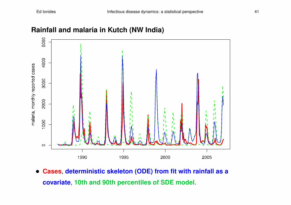
Rainfall and malaria in Kutch (NW India)

• Cases, deterministic skeleton (ODE) from fit with rainfall as a

covariate, 10th and 90th percentiles of SDE model.


The model without rainfall doesn’t capture dynamics

• Cases, deterministic skeleton (ODE) from fitted model without

rainfall, 10th and 90th percentiles of SDE model.


Influenza

• The threat of bird flu (H5N1 influenza) crossing to humans

spurred research into the transmission and evolution of the

influenza virus.

• Descriptive statistical methods show relationships between influenza

transmission, climate and dominant strains (Greene, Ionides & Wilson,

American Journal of Epidemiology, 2006).

• Recent work has used influenza genetic sequence data to study global

transmission and evolution (Rambaut et al., Nature, 2008; Russel et

al., Science, 2008).

• Building a dynamic model describing global transmission and

evolution which is in statistical agreement with genetic and case

report data is an open problem.


Influenza: individual-based models

• Influenza transmission has inspired state-of-the-art statistical

methodology for individual-based population models:

Cauchemez et al (Nature, 2008) inferred transmission parameters

for a partially observed Markov process with a state vector of size

≈ 105, modeling every individual in a small town.

• In climate modeling, it is not unknown to carry out inference with

a state vector of size 107 ( Anderson and Collins, Journal of

Atmospheric and Oceanic Technology, 2007). This requires careful

use of appropriate approximations.


Conclusions

• Plug-and-play statistical methodology permits likelihood-based

analysis of flexible classes of stochastic dynamic models.

• It is increasingly possible to carry out data analysis via nonlinear

mechanistic stochastic dynamic models. This can build links

between the mathematical modeling community (within which models

are typically conceptual and qualitative) and quantitative applications

(testing hypotheses about mechanisms, forecasting, evaluating the

consequences of interventions).

• General-purpose statistical software for partially observed Markov

processes is available in the pomp package for R (on CRAN).


Thank you!

These slides (including references for the citations) are available at

www.stat.lsa.umich.edu/∼ionides/pubs


References

Anderson, J. L. and Collins, N. (2007). Scalable implementations of ensemble filter

algorithms for data assimilation. Journal of Atmospheric and Oceanic Technology,

24:1452–1463.

Breto, C., He, D., Ionides, E. L., and King, A. A. (2009). Time series analysis via

mechanistic models. Annals of Applied Statistics, 3:319–348.

Cauchemez, S., Valleron, A., Boelle, P., Flahault, A., and Ferguson, N. M. (2008).

Estimating the impact of school closure on influenza transmission from sentinel data.

Nature, 452:750–754.

Chen, Y. and Blaser, M. J. (2008). Helicobacter pylori colonization is inversely associated

with childhood asthma. The Journal of Infectious Diseases, 198(4):553–560.

Greene, S. K., Ionides, E. L., and Wilson, M. L. (2006). Patterns of influenza-associated

mortality among US elderly by geographic region and virus subtype, 1968–1998.

American Journal of Epidemiology, 163:316–326.


Grenfell, B. T., Bjornstad, O. N., and Finkenstadt, B. F. (2002). Dynamics of measles

epidemics: Scaling noise, determinism, and predictability with the TSIR model.

Ecological Monographs, 72(2):185–202.

Ionides, E. L., Breto, C., and King, A. A. (2006). Inference for nonlinear dynamical systems.

Proceedings of the National Academy of Sciences of the USA, 103:18438–18443.

Kendall, B. E., Briggs, C. J., Murdoch, W. W., Turchin, P., Ellner, S. P., McCauley, E., Nisbet,

R. M., and Wood, S. N. (1999). Why do populations cycle? A synthesis of statistical and

mechanistic modeling approaches. Ecology, 80:1789–1805.

Kevrekidis, I. G., Gear, C. W., and Hummer, G. (2004). Equation-free: The

computer-assisted analysis of complex, multiscale systems. American Institute of

Chemical Engineers Journal, 50:1346–1354.

Kevrekidis, I. G., Gear, C. W., Hyman, J. M., Kevrekidis, P. G., Runborg, O., and

Theodoropoulos, C. (2003). Equation-free coarse-grained multiscale computation:

Enabling microscopic simulators to perform system-level analysis. Communications in

the Mathematical Sciences, 1:715–762.


King, A. A., Ionides, E. L., Pascual, M., and Bouma, M. J. (2008). Inapparent infections and

cholera dynamics. Nature, 454:877–880.

Liu, J. and West, M. (2001). Combining parameter and state estimation in

simulation-based filtering. In Doucet, A., de Freitas, N., and Gordon, N. J., editors,

Sequential Monte Carlo Methods in Practice, pages 197–224. Springer, New York.

Rambaut, A., Pybus, O. G., Nelson, M. I., Viboud, C., Taubenberger, J. K., and Holmes,

E. C. (2008). The genomic and epidemiological dynamics of human influenza A virus.

Nature, 453:615–619.

Russell, C. A., Jones, T. C., Barr, I. G., Cox, N. J., Garten, R. J., Gregory, V., Gust, I. D.,

Hampson, A. W., Hay, A. J., Hurt, A. C., de Jong, J. C., Kelso, A., Klimov, A. I.,

Kageyama, T., Komadina, N., Lapedes, A. S., Lin, Y. P., Mosterin, A., Obuchi, M.,

Odagiri, T., Osterhaus, A. D. M. E., Rimmelzwaan, G. F., Shaw, M. W., Skepner, E.,

Stohr, K., Tashiro, M., Fouchier, R. A. M., and Smith, D. J. (2008). The global circulation

of seasonal influenza A (H3N2) viruses. Science, 320(5874):340–346.

Sellke, T. (1983). On the asymptotic distribution of the size of a stochastic epidemic.

Journal of Applied Probability, 20:390–394.


Sisson, S. A., Fan, Y., and Tanaka, M. M. (2007). Sequential Monte Carlo without

likelihoods. Proceedings of the National Academy of Sciences of the USA,

104(6):1760–1765.


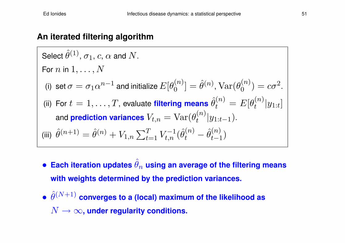
An iterated filtering algorithm

Select θ(1), σ1, c, α and N .

For n in 1, . . . , N

(i) set σ = σ1αn−1 and initialize E[θ(n)

0 ] = θ(n), Var(θ(n)0 ) = cσ2.

(ii) For t = 1, . . . , T , evaluate filtering means θ(n)t = E[θ(n)

t |y1:t]and prediction variances Vt,n = Var(θ(n)

t |y1:t−1).

(iii) θ(n+1) = θ(n) + V1,n∑T

t=1 V −1t,n (θ(n)

t − θ(n)t−1)

• Each iteration updates θn using an average of the filtering means

with weights determined by the prediction variances.

• θ(N+1) converges to a (local) maximum of the likelihood as

N →∞, under regularity conditions.


Iterated filtering via sequential Monte Carlo: A brief tutorial

• Let {XFt,j , j = 1, . . . , J} solve the filtering problem at time t by

having (approximately) marginal density f(xt|y1:t).

• Move particles according to the state process dynamics:

Make XPt+1,j a draw from f(xt+1|xt=XF

t,j). Then {XPt+1,j} is a

draw from f(xt+1|y1:t), solving the prediction problem at time t + 1.

• Prune particles according likelihood given data:

Make XFt+1,j a drawn from {XP

t+1,j} with probability proportional to

wj = f(yt+1|xt+1=XPt+1,j). Then {XF

t+1,j} solves the filtering

problem at t + 1.

• E[xt|y1:t] and Var(xt|y1:t−1) are calculated as the sample mean

and variance of XFt,k and XP

t,k respectively.


Two analogies

• Like the EM algorithm, iterated filtering is an optimization trick that

takes advantage of a special model structure (partially observed

Markov processes).

• Like simulated annealing, iterated filtering introduces stochasticity,

resulting in “thermal fluctuations” which “cool” toward a “freezing point”

at a likelihood maximum.

Documents

Infectious disease dynamics: a statistical perspective ...dept.stat.lsa.umich.edu/~ionides/talks/idd.pdf · Ed Ionides Infectious disease dynamics: ... Infectious disease dynamics: