Inductor Design Methods With Low- Permeability RF Core

Inductor Design Methods With Low-Permeability RF Core Materials

The MIT Faculty has made this article openly available. Please share how this access benefits you. Your story matters.

Citation Han, Yehui, and David J. Perreault. “Inductor Design Methods WithLow-Permeability RF Core Materials.” IEEE Trans. on Ind. Applicat.48, no. 5 (n.d.): 1616–1627.

As Published http://dx.doi.org/10.1109/TIA.2012.2209192

Publisher Institute of Electrical and Electronics Engineers (IEEE)

Version Author's final manuscript

Citable link http://hdl.handle.net/1721.1/87097

Terms of Use Creative Commons Attribution-Noncommercial-Share Alike

Detailed Terms http://creativecommons.org/licenses/by-nc-sa/4.0/

https://libraries.mit.edu/forms/dspace-oa-articles.html

http://hdl.handle.net/1721.1/87097

http://creativecommons.org/licenses/by-nc-sa/4.0/

1

Inductor Design Methods with Low-permeabilityRF Core Materials

Yehui Han, Member, IEEE, and David J. Perreault, Senior Member, IEEE

Abstract—This paper presents a design procedure for inductorsbased on low-permeability magnetic materials, for use in veryhigh frequency (VHF) power conversion. The proposed procedureoffers an easy and fast way to compare different magneticmaterials based on Steinmetz parameters and quickly select thebest among them, to estimate the achievable inductor qualityfactor and size, and to design the inductor. Approximations usedin the proposed methods are discussed. Geometry optimization ofmagnetic-core inductors is also investigated. The proposed designprocedure and methods are verified by experiments.

I. BACKGROUND

There is a growing interest in switched-mode power elec-tronics capable of efficient operation at very high switchingfrequencies (e.g., 10-100 MHz) [1]. Power electronics op-erating at such frequencies include resonant inverters [2]–[11] (e.g., for heating, plasma generation, imaging, and com-munications) and resonant dc-dc converters [2], [4], [12]–[21] (which utilize high frequency operation to achieve smallsize and fast transient response.) These designs utilize mag-netic components operating at high frequencies, and oftenunder large flux swings. These magnetic components shouldhave a high quality factor to achieve high efficiency powerconversion. Unfortunately, most high-permeability magneticmaterials exhibit unacceptably high losses at frequencies abovea few megahertz. There are some low-permeability materials(e.g., relative permeabilities in the range of 4-40) that canbe used effectively at moderate flux swings at frequenciesup to many tens of megahertz [22]–[24]. However, workingwith such low-permeability materials - and the ungapped corestructures they are typically available in - presents somewhatdifferent constraints and challenges than with typical high-permeability low-frequency materials [25]. Because of VHFoperation and the low-permeability characteristics of suchmaterials, the operating flux density is limited by core lossrather than saturation, and a gap is not necessary to preventthe core from saturating in many applications. Without a gap,the core loss begins to dominate the total loss and copperloss can be ignored in many cases. The performance of aVHF magnetic-core inductor thus depends heavily on theloss characteristics of the magnetic material. Moreover, thereappears to be a lack of good design procedures for a selectingamong low-permeability magnetic materials and available coresizes.

Y. Han is with the University of Wisconsin-Madison, 2559C Engi-neering Hall, 1415 Engineering Drive, Madison, WI 53706, USA (email:[email protected]).

D. J. Perreault is with the Laboratory for Electromagnetic and ElectronicSystems, Massachusetts Institute of Technology, Cambridge, MA 02139, USA(e-mail: [email protected]).

This paper, which expands upon an earlier conferencepaper [26], investigates a design procedure for inductors usinglow-permeability magnetic materials. This method is basedon knowledge of the material loss characteristics, such ascollected in [22], [24], and is particularly suited for VHFinductor designs. With the methods developed here, differentmagnetic materials are compared fairly and conveniently, andboth the achievable quality factor and size of a magnetic-coreinductor can be evaluated before the final design.

Section II of the paper introduces the inductor design con-siderations and questions to be addressed. Section III illustratesthe inductor design procedure and methods employed in it.Section IV shows some experimental results to verify thedesign procedure. Section V concludes the paper. In Appen-dices A and B, we check an important assumption behindour methods as well as investigate geometry optimizationproblems of magnetic-core inductors.

II. INDUCTOR DESIGN CONSIDERATIONS AND QUESTIONS

In this paper, we only consider inductor designs under a lim-ited set of conditions in order to make the problem tractable.Nevertheless, these conditions are both very reasonable andpractical for inductors at very high frequencies. The limitedconditions we address are as follows:

1) Use of ungapped cores made of low-permeability mate-rials.

2) Single-layer, foil wound designs in the skin depth limiton toroidal core shapes. A toroidal inductor design keepsmost of flux inside the core, thus reducing EMI/EMCproblems. A foil winding design can further reduce thecopper loss compared to a wire-wound one [27].

3) Design based on knowledge of Steinmetz parametersfor materials of interest. Such parameters are often notpublished or readily available for these materials, butcan be obtained using methods such as that of [22], [24],[28].

4) Design assuming sinusoidal excitation at one frequency.In VHF resonant inverters or converters, inductors oftenhave approximately sinusoidal current at a single fre-quency. Note that consideration of variable frequencyoperation, dc currents, and multiple frequency compo-nents greatly increases complexity of both loss calcula-tion and design [29]–[34].

Fig. 1 shows an inductor has been designed and fabricatedunder the above conditions and replaced the original corelessresonant inductor Ls in a 30 MHz Φ2 inverter [3], [23], [24].The magnetic-core inductor provides a substantial volumetricadvantage over that achievable with a coreless design in thisapplication [23], [24].

IEEE Transactions on Industry Applications, Vol. 48, No. 5, pp. 1616-1627, Sept./Oct. 2012.

2

Ls(a) An example of an inductor fabricated from copper foiland a commercial magnetic core of N40 from CeramicMagnetics.

Ls

(b) Φ2 inverter with the magnetic-core inductor LS

Fig. 1. Photographs of the Φ2 inverter prototype with a magnetic-coreinductor [24].

Given a selection of available cores in different low-permeability materials, and a design specification includinginductance L, current amplitude Ipk, frequency fs, we answerthree important questions about design of VHF inductors underthe above conditions:

1) Which magnetic material from an available set will yieldmaximum quality factor QL for a given size?

2) Given the ability to continuously scale core size, whatmaterial will yield the smallest size for a given qualityfactor QL?

3) For an achievable quality factor QL and inductor size,how should we design the inductor with the selected bestmagnetic material to meet design specifications?

These questions are addressed in the next section.

III. INDUCTOR DESIGN PROCEDURE AND METHODS

A. Inductor Design Procedure

Fig. 2 provides a high-level illustration of the proposeddesign procedure. First, select design specifications from thesystem requirements. Second, select the best magnetic materialfrom a set of low-permeability materials with known Steinmetzparameters. In the third and fourth steps, we estimate theachievable quality factor QL and size of the inductor with thebest available material. If the results are satisfactory, we design

Fig. 2. Inductor design procedure

the inductor. If not, it means the design requirements can’tbe satisfied even with the best available magnetic material,and one must revise the inductor design requirements. A keyfeature of this design procedure is that magnetic materialsare compared first and the best material is selected beforecompleting any individual design, greatly reducing design timeand effort. Some important information such as the maximumquality factor QL, and the smallest possible size can beacquired before the final design. By this procedure, we designan inductor only with one size and one material instead ofinvestigating numerous (perhaps thousands) of combinationsto meet the design specifications.

(1) to (3) are used often in our design procedure. In VHFpower conversion, ac losses (conductor/copper and core losses)usually dominate and we thus ignore dc losses (conductor loss)here. In (1) and (2), we use the quality factor QL to evaluatethe ac losses of an inductor at a single frequency. Rac isthe equivalent total ac resistance of a magnetic-core inductorincluding copper loss and core loss, Rcu is the equivalentresistance owing to copper loss, and Rco is an equivalentresistance owing to core loss. The Steinmetz equation is anempirical means to estimate loss characteristics of magneticmaterials [35], [36]. It has many extensions [29]–[34], [36]–[38], but we only consider the formulation for sinusoidal driveat a single frequency here. In (3), Bpk is the peak amplitudeof average (sinusoidal) flux density inside the material andPV is power loss per unit core volume 1. K and β arecalled Steinmetz parameters. K and β have been calculated

1Use of average flux density in the core simplifies the calculations. Fortypical core sizes, this approximation is well justified, and the error of thisapproximation should be lower than 10% as shown in Appendix A. (Fluxnonuniformity for other cases is treated in [39], [40], for example.)


3

for several commercial low-permeability rf magnetic materialsfrom 20 MHz to 70 MHz in [22], [24], [28].

QL =ωL

Rac(1)

Rac = Rcu +Rco (2)

PV = KBβpk (3)

B. Method to Select Among Magnetic Materials

In the second step of the design procedure, we identify thebest material. We begin with a coreless inductor to make acomparison among different design options (including mag-netic materials) for a given L, Ipk, fs, minimum QL andmaximum size limitation. Ignoring the “single-turn” induc-tance associated with the circumferential current componentaround the core [27], the number of turns Nair for a corelessinductor can be calculated from (4) [27]:

Nair ≈√√√√ 2πL

hµ0 ln(dodi

) (4)

do, di and h are the outside diameter, inside diameter andheight of the coreless inductor. The approximate average fluxdensity Bpk−air inside the core is calculated by (5):

Bpk−air =µ0NairIpk

0.5π(di + do)(5)

Likewise, the number of turns N and average flux density Bpkof a magnetic-core inductor are calculated by (6) and (7) 2:

N ≈√√√√ 2πL

hµ0µr ln(dodi

) (6)

Bpk =µ0µrNIpk

0.5π(di + do)= µ0.5

r Bpk−air (7)

For a given L and specified dimensions in (7), average fluxdensity Bpk inside the core may be different for each magneticmaterial, which is one of the reasons we can’t compare theirloss characteristics for different magnetic materials directlyat the same flux density level. However, we propose here amethod by which direct comparisons can be made: Bpk of eachmagnetic material can be normalized to the coreless inductorflux density Bpk−air by its relative permeability µr. For agiven design specification, all magnetic materials will havethe same normalized flux density, which is equal to µ−0.5r Bpk.Given a set of Steinmetz parameters, we can draw the curvesof PV vs. µ−0.5r Bpk for all available magnetic materials. Wecompare PV of these materials at µ−0.5r Bpk = Bpk−air anddecide which material has the smallest core loss for the givendesign specification.

An example is shown in Fig. 3, in which we considera design of a magnetic-core inductor at Ipk = 2 A and

2The relative permeability can be also addressed in a complex form whichis equal to µ′r − µ′′r j. µ′r is equal to µr in (6) and (7) and µ′′r representsthe loss which is also a function of flux density. µ′′r can be calculated fromthe core loss measurement results in [24]. In this paper, we use curves andSteinmetz parameters to represent losses instead of complex permeability.

1.0 1.3 1.6 2.0102

103

104

μr−0.5Bpk − AC Flux Density Amplitude (mT)

PV (

mW

/cm

3 )

M3P67N40

Pv=614 mW/cm3

Fig. 3. Inductor design example (do = 12.7 mm, di = 6.3 mm, h =6.3 mm, L = 200 nH, Ipk = 2 A, fs = 30 MHz and Bpk−air = 1.3 mT).

fs = 30 MHz with L = 200 nH and maximum sizedo = 12.7 mm, di = 6.3 mm and h = 6.3 mm 3. Beginningwith a coreless inductor, we calculate Bpk−air = 1.3 mT from(4) and (5). Using data from [22], [24], loss curves of PV vs.µ−0.5r Bpk are plotted for the materials N40, P, M3 and 67 4.We compare their PV at Bpk−air and find that N40 materialhas the smallest core loss (614 mw/cm3). If we ignore thecopper loss, the magnetic-core inductor with N40 materialwill achieve the highest QL for given design specifications.We can also observe in Fig. 3 that N40 is better than the othermagnetic materials and 67 is worse than the others over a widerange of flux density. This will help us to design a magnetic-core inductor if its operating current level is unknown or verywide.

So far, we still don’t know if the magnetic-core inductorwith the best material is better than a coreless inductor of thesame size. There is no core loss and Steinmetz parametersfor a coreless inductor. But we can still compare its copperloss to core losses of other magnetic materials on the samegraph. To accommodate the coreless design, we define PV−airat Bpk−air as the power loss per unit volume for a corelessinductor and calculate it by (8):

PV−air =Rcu−air

2VI2pk (8)

Rcu−air is the copper resistance of a coreless inductor andV is the volume of the coreless inductor. Rcu−air (or thecopper resistance of a magnetic-core inductor Rcu) dependsheavily on a coreless or magnetic-core inductor windingdesign pattern. One could find the ac resistance of a corelessinductor by constructing and measuring it or simulating it

3Examples in the paper are confined to 30MHz. However, the same designprocedure can be applied to a broader range of frequencies.

4-17 material in [22], [24] has a very low relative permeability and low coreloss characteristics. Compared to its core loss, the copper loss of -17 materialcan’t be ignored. As a special case, -17 is not considered here. However, themethods introduced in this paper can still be applied for -17 material withspecial considerations of its copper loss.


4

1.0 1.3 1.6 2.0102

103

104


PV (

mW

/cm

3 )

M3P67N40

Pv-air=1073 mW/cm3

Pv=614 mW/cm3

Fig. 4. Inductor design example including the power loss characteristic of acoreless inductor (do = 12.7 mm, di = 6.3 mm, h = 6.3 mm, L = 200 nH,Ipk = 2 A, fs = 30 MHz and Bpk−air = 1.3 mT).

using computational techniques. Alternatively, the resistancecan be estimated for different design variants:

1) In [22], [24], the windings are made of an equal-widthfoil-like conductor, and Rcu−single−turn is the ac copperresistance of a single turn inductor:

Rcu = N2Rcu−single−turn

≈ N2 ρcuπδcu

(2h

di+dodi− 1

)(9)

2) In [22], [24], Rcu can alternatively be estimated fromthe foil width, length and skin depth:

Rcu ≈ρculcuδcuwcu

(10)

3) In [27], the windings are made of foil-like conductortapered to conform to the shape of the toroid:

Rcu = N2Rcu−single−turn

≈ N2 ρcuπδcu

(h

di+

h

do+ 2 ln

dodi

)(11)

For example, the loss characteristics of a coreless inductorestimated by (9) is included in Fig. 4 . We can see N40 is theonly magnetic material which has lower loss than the corelessinductor. Thus the magnetic-core inductor built with N40 mayhave a higher quality factor QL than the coreless inductor. Themagnetic-core inductor built with other materials (e.g. M3, Pand 67) will not be better than the coreless inductor and neednot be considered in the following steps. Here, we can see thatthis comparison lets us exclude most of available magneticmaterials in the pool from the design, saving time and effort.

From previous measurements in [22], [24], the core loss(Rco) usually dominates the total loss of an ungapped VHFmagnetic-core inductor. However, this statement should bechecked to make sure that it is still correct for an individualdesign. By a similar method, we can define the copper loss

1.0 1.3 1.6 2.0101

102

103

104


PV (

mW

/cm

3 )

M3P67N40

Pv=614 mW/cm3

Pv-cu=72 mW/cm3

Fig. 5. Inductor design example including the copper loss characteristic ofa magnetic-core inductor (do = 12.7 mm, di = 6.3 mm, h = 6.3 mm,L = 200 nH, Ipk = 2 A, fs = 30 MHz and Bpk−air = 1.3 mT).

per unit volume PV−cu of a magnetic-core inductor and markit on the graph of PV vs. µ−0.5r Bpk. From (4) and (6),

N = µ−0.5r Nair (12)

Rcu = N2Rcu−single−turn = µ−1r Rcu−air (13)

PV−cu =Rcu2V

I2pk =µ−1r Rcu−air

2VI2pk = µ−1r PV−air (14)

PV−air can be calculated from (8). The copper loss character-istic of a magnetic-core inductor for the example specificationsbuilt in N40 magnetic material is marked in Fig. 5. In thisexample, the copper loss of the magnetic-core inductor is muchsmaller than its core loss (an order of magnitude or more 5).

C. QL Estimation with Given Maximum Inductor Size

In the third step of the design procedure in Fig. 2, weestimate the highest quality factor that can be achieved. Ifwe ignore the copper loss comparing to the core loss of themagnetic-core inductor, the quality factor QL can be estimatedby (15) and (16):

Rco ≈Total Core Loss

0.5I2pk=

PV V

0.5I2pk(15)

QL ≈ωL

Rco= ωL

0.5I2pkPV V

(16)

E.g., for the magnetic-core inductor built in N40, PV =614 mW/cm3 at Bpk−air = 1.3 mT, and QL ≈ 198 by (16).In this example Rco ≈ 0.19 Ω and Rcu ≈ 0.03 Ω, whereRco Rcu. QL can also be estimated by (2), in which copperloss is included, and QL ≈ 171 by (2).

5We note that the simple copper loss calculations of (9) in a cored inductordesign may have up to 30% error [22], [24], but this degree of accuracy issufficient for our present purposes.


5

D. Size Estimation with Given Minimum QL

In this subsection, we illustrate the third step in our inductordesign procedure, estimating minimum achievable inductorsize for a required quality factor. Because the method in-troduced in this subsection is not as simple and direct asthe method in Section III-B, we begin this subsection with ageneral description of the method. Then we derive equationsneeded in our method for inductor size estimation. As we havedone in Section III-B, step by step design examples are givento aid understanding of the method.

We again begin with a coreless inductor design, calculate itssize and compare the size of a magnetic-core inductor with it.In our method, we define the scaling factor λ as the dimensionratio of a magnetic-core inductor and the coreless inductor forgiven L, QL, fs and Ipk, and we assume that the relativeratio of the 3 dimensions is kept constant during the scaling.Thus, we scale each dimension (x, y, z) describing the shapeof the coreless inductor by a factor λ to get the correspondingdimension of a magnetic-core inductor: the coreless inductorthus has λ = 1, and the magnetic-core inductor with theminimum λ has the smallest size.

Our method has four main steps:1) Given L, Ipk, fs and minimum required QL, design a

coreless inductor and get its dimension parameters do,di, h.

2) Calculate Bpk−air of the coreless inductor, compare itsPV−air to PV of other magnetic materials at Bpk−air onthe graph of PV vs. µ−0.5r Bpk and decide the possiblebest materials for the inductor design.

3) Calculate the scaling factor λ for the possible bestmaterials.

4) Check the flux density B′pk, core loss PV ′ , and copperloss PV ′−cu of the magnetic-core inductor after scalingon the graph of PV vs. µ−0.5r Bpk.

1) Step I, Calculate Coreless Design: From (4), the qualityfactor QL of a coreless inductor can be calculated by (17):

QL =ωL

Rcu−air=

µ0fsRcu−single−turn

h ln

(dodi

)(17)

Rcu−single−turn can be estimated by (9) or (11).If we assume di = 0.5do, we can solve the dimension

parameters do, di, h of a coreless inductor from (9)/(11), and(17) for given fs, QL and ratio of h and do. In Appendix B, weshow that this assumption is very reasonable because lettingdi = 0.5do yields an inductor with nearly optimum QL andthus the smallest size.

2) Step II, Evaluate Magnetic Materials: After calculatingthe dimensions of the coreless inductor, its Bpk−air andPV−air can be calculated by (5) and (8). PV at Bpk−air ofall the magnetic materials can be found from the graph ofPV vs. µ−0.5r Bpk. For example, we consider the design of acoreless inductor with L = 200 nH, Ipk = 2 A, fs = 30 MHz,and QL = 116. We define this coreless inductor as havingλ = 1. Its dimensions are do = 12.7 mm, di = 6.3 mm andh = 6.3 mm. The question we seek to answer is: if we buildan inductor with magnetic materials, how small it could bewhile achieving the specified minimum QL. We first calculate

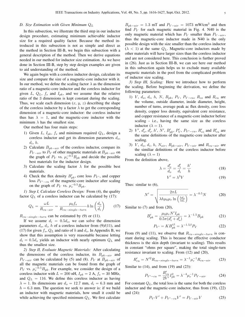
Bpk−air = 1.3 mT and PV−air = 1073 mW/cm3 and thenfind PV for each magnetic material in Fig. 4. N40 is theonly magnetic material which has PV smaller than PV−air,thus the magnetic-core inductor made in N40 is the onlypossible design with the size smaller than the coreless inductor(λ < 1) at the same QL. Magnetic-core inductors made byother materials will have larger sizes than the coreless inductorand are not considered here. This conclusion is further provedin (26). Just as in Section III-B, we can see here our methodin this subsection again helps us to exclude many availablemagnetic materials in the pool from the complicated problemof inductor size scaling.

3) Step III, Scaling: Here we introduce how to performthe scaling. Before beginning the derivation, we define thefollowing parameters:

1) V , do, di, h, N , Bpk, PV , PV−cu, Rco and Rcu arethe volume, outside diameter, inside diameter, height,number of turns, average peak ac flux density, core lossdensity, copper loss density, equivalent core resistance,and copper resistance of a magnetic-core inductor beforescaling - i.e., having the same size as the corelessinductor (λ = 1).

2) V ′, d′o, d′i, h′, N ′, B′pk, P ′V , PV ′−cu, R′co and R′cu are

the same definitions of the magnetic-core inductor afterscaling.

3) V , do, di, h, Nair, Bpk−air, PV−air and Rcu−air arethe similiar definitions of the coreless inductor beforescaling (λ = 1)

From the definition above,

λ =d′odo

=d′idi

=h′

h(18)

V ′ = λ3V (19)

Thus: similar to (6),

N ′ =

√√√√ 2πL

λhµ0µr ln(λdoλdi

) = λ−0.5N (20)

Similar to (7) and from (20),

B′pk =µ0µrN

′Ipk0.5π(d′i + d′o)

= λ−1.5Bpk (21)

PV ′ = KB′βpk = λ−1.5βPV (22)

From (9) and (11), we observe that Rcu−single−turn is con-stant during scaling. This is because the effective conductorthickness is the skin depth (invariant to scaling). This resultsin constant “ohms per square”, making the total single-turnresistance invariant to scaling. From (12) and (20),

R′cu = N ′2Rcu−single−turn = λ−1µ−1r Rcu−air (23)

Similar to (14), and from (19) and (23):

PV ′−cu =R′cu2V ′

I2pk = λ−4µ−1r PV−air (24)

For constant QL, the total loss is the same for both the corelessinductor and the magnetic-core inductor, thus from (19), (22)and (24):

PV ′V′ + PV ′−cuV

′ = PV−airV (25)


6

1.0 10.010

1

102

103

104

105

106

107

µr−0.5Bpk − AC Flux Density Amplitude (mT)

PV (

mW

/cm

3 )

M3P67N40

Pv=614 mW/cm3

Pv-cu=72 mW/cm3

Pv-air=1073 mW/cm3

Pv'=133590 mW/cm3

Pv'-cu=85650 mW/cm3

1.3 18.5

Fig. 6. The magnetic-core inductor after scaling design

λ3−1.5βPV

PV−air+ λ−1µ−1r = 1 (26)

The scaling factor λ can be calculated by (26), if we knowPV , relative permeability µr, and Steinmetz parameter β ofthe magnetic material, and PV−air of the coreless inductor.Because of the usual case for Steinmetz parameters (e.g., β >2), PV should be smaller than PV−air to get λ < 1 from(26). This explains why we don’t have to consider magneticmaterials which have PV larger than PV−air. (26) is the keyequation for calculating achievable design scaling at constantQL through the use of an ungapped magnetic core.

Let’s continue our example shown in Fig. 4. For N40material, PV = 614 mw/cm3 at Bpk−air = 1.3 mT, β = 2.02at 30 MHz and µr = 15, the scaling factor λ = 0.17 bysolving (26).

4) Step IV, Check Design Assumptions: As a last step, wecheck the flux density B′pk, core loss P ′V , and copper lossPV ′−cu of the inductor after scaling on the graph of PV vs.µ−0.5r Bpk. From (7) and (21):

µ−0.5r B′pk = λ−1.5Bpk−air (27)

In the example, P ′V = 1.3 × 105 mW/cm3 by (22) andP ′V−cu = 8.6 × 104 mW/cm3 by (24) are shown in Fig. 6.We can still see that the core loss dominates the total loss.With completion of this last step, we now have an inductorgeometry and scaling that achieves the smallest size at therequired QL.

5) Inductor Scaling with Multiple choices of MagneticMaterials: Here we give an example of the solution whenthere is more than one possible material which can be usedto build a cored inductor having smaller size than the corelessinductor and thus λ < 1.

We consider the design of a coreless inductor with L =200 nH, Ipk = 0.5 A, fs = 30 MHz, and QL = 116. Wedesign a coreless inductor which has λ = 1 and dimensionsof do = 12.7 mm, di = 6.3 mm and h = 6.3 mm. We firstlycalculate Bpk−air = 0.32 mT and PV−air = 67 mW/cm3

and then find PV for each magnetic material in Fig. 7. P, M3

0.3 0.32 0.36 0.40 0.44 0.5010

1

102

103


PV (

mW

/cm

3 )

M3P67N40

Pv-air=67.0 mW/cm3

P: Pv=57.1 mW/cm3

N40: Pv=37.3 mW/cm3

M3: Pv=16.9 mW/cm3

Fig. 7. Loss plots of inductor design scaling example (do = 12.7 mm,di = 6.3 mm, h = 6.3 mm, L = 200 nH, Ipk = 0.5 A, fs = 30 MHz andBpk−air = 0.32 mT).

and N40 are magnetic materials which have PV smaller thanPV−air, thus magnetic-core inductors made with these threematerials may possibly be smaller than the coreless inductor(λ < 1). Because P material has both a larger core loss PVand a larger slope (= β) of the loss curve than N40 material atBpk−air, we can immediately conclude that P material will notbe competitive with N40 material for this design. However, wecan’t immediately determine which of M3 and N40 materialsis better: M3 has a lower PV at Bpk−air but a higher slope ofthe loss curve than N40. We thus consider both M3 and N40as possible best materials and calculate their scaling factor λby (26). We list the calculation results in Table I which alsoincludes P material to confirm our conclusion. From Table I,we can see that the magnetic-core inductor built with N40 stillhas the smallest scaling factor for the specified minimum QL,and represents the best design choice.

TABLE ICOMPARISON OF SCALING FACTOR λ AMONG MAGNETIC-CORE

INDUCTORS BUILT WITH P, M3 AND N40 MATERIALS.

Material P M3 N40

PV (mW/cm3) 57.1 16.9 37.3

µr 40 12 15

β 2.33 3.24 2.02

λ by (26) 0.77 0.52 0.16

We check the flux density B′pk, core loss P ′V , and copperloss PV ′−cu of the scaled magnetic-core inductor built withN40 material on the graph of PV vs. µ−0.5r Bpk by (22),(24) and (27). In the example, the scaled design operatesat a normalized flux density µ−0.5r B′pk = 5.0 mT, P ′V =9621 mW/cm3, and P ′V−cu = 6819 mW/cm3 as illustratedin Fig. 8. We can see that the core loss of N40 is the lowestamong the materials at this normalized flux density of theN40 design. If we build a magnetic-core inductor with othermaterials with the same size after scaling, the inductor will


7

0.2 0.3 0.5 1.0 2.0 3.0 5.010

0

101

102

103

104

105

106


PV (

mW

/cm

3 )

M3P67N40

Pv-air=67.0 mW/cm 3

Pv=37.3 mW/cm3

Pv-cu=4.5 mW/cm3

Pv'-cu=6819 mW/cm3

Pv'=9621 mW/cm3

Fig. 8. The magnetic-core inductors after scaling

have a lower quality factor and must have a bigger size tosatisfy the design requirement for minimum quality factor;this confirms our conclusion that the magnetic-core inductorbuilt with N40 will have the smallest size.

E. Inductor Design with the Best Magnetic Material

Having satisfied quality factor QL and inductor size re-quirements, the inductor can be designed with the selectedbest magnetic material (N40). To provide a complete answerfor the previous design example, we summarize the results ofeach step in Fig. 2:

1) We give the design requirements: L = 200 nH, Ipk =2 A, fs = 30 MHz, minimum QL = 116 and maximumsize of do = 12.7 mm, di = 6.3 mm and h = 6.3 mm.

2) Given available magnetic materials (67, P, M3 and N40)and their Steinmetz parameters, we determine that N40is the best material for design.

3) Given the maximum size, estimate the highest QL of amagnetic-core inductor with N40 material (about QL =171).

4) Given the minimum QL, estimate the scaling factor λ =0.17 and the minimum size do = 2.2 mm, di = 1.1 mmand h = 1.1 mm calculated by (18).

5) We check the results in the third and fourth steps andsee if they satisfy the design requirements.

6) If we prefer a core inductor with the highest QL at themaximum size, the inductor will have a number of turnsN = 4 calculated by (6), an inductance L = 199 nH,and a core size of do = 12.7 mm, di = 6.3 mm andh = 6.3 mm. Its quality factor QL has been estimatedin Section III-C as 198 neglecting copper loss and 171including copper loss. If we prefer a cored inductorwith the minimum size at the minimum allowed QL of116, the inductor will have a number of turns N ′ = 10calculated by (20) and the core size is do = 2.2 mm,di = 1.1 mm and h = 1.1 mm.

Compared to a coreless design, the magnetic-core inductorwith N40 material will have 47% higher quality factor QL for

the same maximum size or 83% size reduction for the sameminimum quality factor.

F. Relationship between Quality Factor QL and Inductor Size

The method to calculate the scaling factor λ proposed inSection III-D has two shortcomings: the first is that we mayneed to rely on some numerical methods to solve the nonlinearequation (26), and the second is that it doesn’t reveal therelationship of a magnetic-core inductor’s quality factor andits size in a direct and intuitively understandable way. Inthis subsection, we study the inductor’s quality factor as thefunction of its scaling factor λ.

We again begin our derivations with a coreless inductor. Wedefine quality factor QL0 with given maximum size (λ = 1)and calculate it by the following equation:

QL0 =ωL

Rcu−air=

µ0f

Rcu−single−turnh ln

(dodi

)(28)

Because Rcu−single−turn is constant during the scaling as de-scribed before, the quality factor after scaling can be calculatedby the following equation:

QL(λ) =ωL

Rcu=

µ0f

Rcu−single−turnhλ ln

(doλ

diλ

)= λQL0 (29)

From (29), we can see there is a linear functional relationshipbetween quality factor QL and scaling factor λ for a core-less inductor. This general result for coreless design is wellknown; see the classic scaling rules for coreless solenoids, forexample [1], [41]–[44]. For a magnetic-core inductor, from(23),

R′cu = λ−1µ−1r Rcu−air =ωL

λµrQ0(30)

From (19) and (22),

R′co =PV ′V

′

0.5I2pk=λ3−1.5βPV V

0.5I2pk= λ3−1.5β

PVPV−air

PV−airV

0.5I2pk

= λ3−1.5βPV

PV−airRcu−air = λ3−1.5β

PVPV−air

ωL

QL0(31)

From (30) and (31),

QL(λ) =ωL

R′cu +R′co=

QL01λµr

+ λ3−1.5β PV

PV−air

(32)

Starting from a baseline design, from (29) and (32), we canplot QL vs. λ for magnetic-core inductors made in all availablemagnetic materials, as well as for a coreless inductor. Anexample is shown in Fig. 9. The baseline design specificationsare L = 200 nH, Ipk = 2 A, f = 30 MHz, and QL = 116. Atλ = 1, the coreless inductor has dimensions do = 12.7 mm,di = 6.3 mm and h = 6.3 mm. For a given QL, we can useresults such as in Fig. 9 to find its scaling factor λ and furtherdecide the inductor size for every magnetic material using (18).Moreover, for a given size (scaling factor λ), we can find thequality factor QL that is achievable for each material.

While this approach to explore inductor scaling and sizingis informative, it still has some shortcomings. The first one


8

0.1 0.2 0.4 0.6 0.8 1.0100

101

102

103

Scaling Factor λ

Qua

lity

Fact

or Q

L

M3P67N40Coreless

Fig. 9. QL vs. λ for coreless inductor and magnetic-core inductors indifferent mangetic materials (L = 200 nH, Ipk = 2 A and f = 30 MHz). Atλ = 1, the coreless inductor has the dimensions do = 12.7 mm, di = 6.3 mmand h = 6.3 mm.

is that we have to generate a new graph by (29) and (32)for each baseline design of interest. The second one is thatwe can’t a priori exclude some magnetic materials fromconsideration as we did in Section III-D. If we have dozensof magnetic materials, the graph of QL vs. λ will becomevery complicated. The third one is that all these materials arecompared on the graph at a fixed current level and not overa wide operating range. Nevertheless the methods illustratedhere provide a better view into design tradeoffs than oneotherwise available.

IV. EXPERIMENTAL VERIFICATION

We carried out several experiments to verify the designprocedure illustrated in this paper. Firstly, we want to verifythe design steps 2 and 3 in Fig. 2. That is, given availablemagnetic materials and design requirements (inductance L,current amplitude Ipk, and frequency fs), we want to de-termine the best material to yield maximum quality factorQL for a given size, and estimate the highest QL that canbe achieved at that size. Design parameters for the exampleapplication are repeated here: do = 12.7 mm, di = 6.3 mm,h = 6.3 mm, L = 200 nH, Ipk = 2 A, and fs = 30 MHz.As predicted in our design procedure, N40 is the best materialand the magnetic-core inductor with N40 has quality factorQL = 171. We designed and fabricated a magnetic-coreinductor with copper foil and N40 core to satisfy the designspecifications, and measured its inductance and quality factorwith the experimental methods in [22]. To make comparisonswith other designs, we fabricated a coreless inductor andmagnetic-core inductors with 67, M3 and P materials andsimilar core sizes. The results are listed and compared inTable II. The cores in M3 and P materials have di larger thanthe design specification, e.g. dido = 0.62 vs. 0.50. The core lossestimation error due to this is small loss less than 4% higheras shown in Fig. 11 in Appendix B. The core in 67 materialhas a di larger and h lower than the design specifications, and

its volume is thus 71.4% of the specified one. The core lossestimation error due to this is only 3.1% higher calculated by(48) where β = 2.18 [22]. We can see the measurement resultsfit very well with the predicted values and the magnetic-coreinductor with N40 material is the best design compared toothers as we have predicted in our design procedure. To someextent, these results also verify the results of approximationand optimizations shown in Appendices A and B.

TABLE IICOMPARISON AMONG CORELESS INDUCTORS AND MAGNETIC-CORE

INDUCTORS DESIGNED AT Ipk = 2 A AND fs = 30 MHZ IN DIFFERENT

MAGNETIC MATERIALS.

Material N40 M3 P 67 Coreless

Suppliers CeramicMag-netics

NationalMagneticsGroup

Ferro-nics

Fair-rite

N/A

Permeability 15 12 40 40 1

Designations T5025-25T

998 11-250-P

59670-00301

N/A

do (mm) 12.7 12.7 12.7 12.7 12.7

di (mm) 6.3 7.9 7.9 7.2 6.3

h (mm) 6.3 6.4 6.4 5.0 6.3

Turns Number N 4 5 3 3 14

Predicted L (nH) 199 180 219 203 173

Measured L (nH) 230 181 262 235 245

Predicted QL 171 74 81 39 116

Measured QL 167 65 87 45 96

Secondly, we verified the design step 4 illustrated in Sec-tion III-D. That is, given L, Ipk, fs and the minimum QL,determine the best material for design and estimate the mini-mum size achievable for that QL requirement. This experimentis much more difficult than the first one because limited avail-ability of core sizes. If we design a magnetic-core inductorwith N40 material which has the scaling factor λ = 0.17 ascalculated in Section III-D, the inductor after scaling has 10turns and dimensions d′o = 2.16 mm, d′i = 1.07 mm andh′ = 1.07 mm. The winding of copper foil has a width ofless than 0.34 mm! It is very hard to wind such a narrowcopper foil on this tiny core by hand. The magnetic-coreinductor with P material in Section III-D5 has a higher scalingfactor λ and thus a larger core size after scaling. So forsimplicity, we verified the design of P material instead ofN40. The design parameters are repeated here: L = 200 nH,Ipk = 0.5 A, fs = 30 MHz and QL = 116. The scaling factorλ = 0.77 calculated by (26) and shown in Table I. The coredimensions after scaling are d′o = 9.78 mm, d′i = 4.85 mmand h′ = 4.85 mm. The available core with the closest size hasdimensions d′o = 9.63 mm, d′i = 4.66 mm and h′ = 3.21 mm.We designed and fabricated a 3-turn magnetic-core inductorwith P material and measured its inductance L and qualityfactor QL. The results are shown in Table III. We can see themeasurement results fit very well with the predicted value (forthe actual size) and (26) is thus verified.

Thirdly, we verified (32) and the relationship of QL vs. λshown in Fig. 9. The design parameters are repeated here: L =200 nH, Ipk = 2 A and fs = 30 MHz. At λ = 1, the corelessinductor has the dimensions do = 12.7 mm, di = 6.3 mm


9

TABLE IIIMAGNETIC-CORE INDUCTOR DESIGNED AT L = 200 NH, Ipk = 0.5 A

AND fs = 30 MHZ WITH THE SCALING FACTOR λ = 0.77.

Material P Designation 11-220-PTurns Number N 3 d′o (mm) 9.63

d′i (mm) 4.66 h′ (mm) 3.21

Predicted L (nH) 168 Measured L (nH) 181

Predicted QL 110 Measured QL 105

and h = 6.3 mm. We design a magnetic-core inductor withN40 material and scaling factor λ = 0.5. The magnetic-coreinductor after scaling thus has dimensions d′o = 6.35 mm,d′i = 3.15 mm and h′ = 3.15 mm. The closest available coresize has the dimensions d′o = 5.84 mm, d′i = 3.05 mm andh′ = 4.06 mm. We designed and fabricated a 5-turn magnetic-core inductor with N40 materials and measure its inductanceL and inductor quality factor QL. The results are shown inTable IV. We can see the measurement results fit very wellwith predicted value (for the actual size) and thus (26) andFig. 9 are verified.

TABLE IVMAGNETIC-CORE INDUCTOR DESIGNED AT L = 200 NH, Ipk = 2 A AND

fs = 30 MHZ WITH THE SCALING FACTOR λ = 0.5.

Material N40 Designation T231216TTurns Number N 5 d′o (mm) 5.84

d′i (mm) 3.05 h′ (mm) 4.06

Predicted L (nH) 198 Measured L (nH) 180

Predicted QL 160 Measured QL 154

V. CONCLUSION

In this paper, we propose an inductor design procedureusing low permeability magnetic materials. The design pro-cedure is based on the use of Steinmetz parameters and low-permeability ungapped cores. With this procedure, differentmagnetic materials are compared fairly and fast, and both thequality factor QL and the size of a magnetic-core inductorcan be predicted before the final design. We also compare amagnetic-core inductor design to a coreless inductor design inour design procedure. Some problems, such as optimizationof magnetic-core inductors, are also investigated in this paper.The procedure and methods proposed in this paper can help todesign magnetic-core inductors with low-permeability rf corematerials.

APPENDIX AAPPROXIMATIONS USED IN THE PROPOSED METHODS

In Section III, we average the flux density inside a toroidalcore to simplify our calculations. Because the flux densityinside a toroidal core is actually not uniform, we need toknow if our approximation is reasonable. For a magnetic-coreinductor, the average flux density is:

Bpk =µ0µrNIpk

0.5π(do + di)=

Ipk0.25(do + di)

√√√√ µ0µrL

2πh ln(dodi

) (33)

The average total core loss:

P (di) = PV V = KBβpkπ

[(do2

)2

−(di2

)2]h =

πhK

Ipk0.25(do + di)


2πh ln(dodi

)β [(

do2

)2

−(di2

)2]

(34)

The total core loss P0 is calculated without the approximationof uniform flux. From (6),

Bpk(r) =µ0µrNIpk

2πr=Ipkr


2πh ln(dodi

) (35)

Where r specifies a radius from the center of the core (di2 <r < do

2 ).

P0(di) =

∫ do2

di2

PV dV =

∫ do2

di2

KBpk(r)β2πrhdr

= 2πhK

Ipk√√√√ µ0µrL

2πh ln(dodi

)β ∫ do

2

di2

r1−βdr (36)

If β 6= 2,

P0(di) =2πhK

2− β


2πh ln(dodi

)β [(

do2

)2−β

−

(di2

)2−β]

(37)

If β = 2,P0(di) = µ0µrKLI

2pk (38)

We compare P0 and P and define the error by the followingequation:

Error = 1− P (di)

P0(di)(39)

from (34) and (37), if β 6= 2,

Error = 1− (2− β)2β−1

[1−

(dido

)2](1 + di

do

)−β1−

(dido

)2−β (40)

from (34) and (38), if β = 2,

Error = 1− 21−

(dido

)2(

1 + dido

)2ln(dodi

) (41)

We can see Error only depends on the magnetic materialSteinmetz parameter β and the dimension ratio of di to do.Error is plotted in Fig. 10 for different di

doand β. We can

see it is below 10% if β is less than 3 and dido> 0.52 which

is typical for most of available commercial magnetic cores.We assume an optimum di ≈ 0.5do later. So the error of thisapproximation should be lower than 10%, which is reasonable.


10

0 0.2 0.4 0.6 0.8 10

10

20

30

40

50

di / d

o

Err

or %

β=2.0β=2.2β=2.4β=2.6β=2.8β=3.0

Fig. 10. The error of average flux density approximation.

APPENDIX BOPTIMIZATION OF MAGNETIC-CORE INDUCTORS

In Section III, different magnetic materials are comparedand evaluated with the assumption that optimum magnetic-core inductors made in all these materials will have the samerelative dimensions as the coreless design on which they arebased. However, magnetic-core inductors may have their ownrelative optimum dimensions for the maximum quality factorQL or the minimum size for different materials, thus themethods proposed in Section III may not be a fair comparison.That is, we need to establish whether or not the best shapefor an inductor changes significantly with scale or materialcharacteristics.

As will be seen, the results are quite reasonable and theapproaches of Section III lead to near optimum designs undera wide range of conditions. We consider two optimizationcases in this paper. First, we assume that a toroidal magnetic-core inductor’s do and h are restricted to be constant (e.g., asstipulated by the specification of a power electronics circuit),and we optimize di to get the maximum quality factor QL.Second, we assume its volume V is restricted to be constant,and we optimize do, di and h to get the maximum qualityfactor QL. In all the optimizations, make the assumption thatcore losses dominate and neglect copper loss. We do take intoaccount the fact that the flux density inside the core is notuniform when calculating core loss.

A. Optimization of di at Fixed do and h

From (37) and (38), let di = 0.5do and we normalize thetotal core loss P0(di) by the total loss P0 at di = 0.5do. Ifβ 6= 2,

P0(di)

P0(0.5do)=

ln 2

ln(dodi

)0.5β

1−(dido

)2−β1− 0.52−β

(42)

If β = 2,P0(di)

P0(0.5do)= 1 (43)

0 0.2 0.4 0.6 0.8 10.98

1

1.02

1.04

1.06

1.08

1.1

di / d

o

P(d

i) / P

(0.5

d o)

β=2.0β=2.2β=2.4β=2.6β=2.8β=3.0

00

Fig. 11. Plot of core power loss dissipation in a rectangular cross-sectiontoroidal core as a function of di

do, normalized to that with di

do= 0.5. Results

are parameterized in Steinmetz parameter β. It can be seen that over a widerange of β, di

do= 0.5 is very close to the optimum, and that results are not

highly sensitive to dodi

.

In (42), P0(di)P0(0.5do)

only depends on the ratio of dodi

andSteinmetz parameter β. We plot P0 as a function of do

difor

different β in Fig. 11. From Fig. 11, we can see that theoptimum di is around 0.4do, with an exact value that dependson β. When di varies between 0.22do and 0.64do, the totalcore loss P is very flat and the deviation from the minimumcore loss is less than 10%. We choose di = 0.5do instead ofdi = 0.4do for the following considerations: firstly, di = 0.5dois a more typical dimension ratio for commercial magneticcores (e.g., see Table II); secondly, as shown in AppendixA, the error due to the assumption of average flux densityis less than 10% if di ≥ 0.5do. The error in assumingthat the optimum inside diameter is di = 0.5do is lowerthan 2% for a wide range of β values. So we can thinkdi = 0.5do as the nearly-optimum dimension for a wide rangeof magnetic materials. We can thus compare and evaluatedifferent magnetic materials under the same dimensions andour assumption in Section III is correct.

B. For a Constant Volume V , Optimization of Dimensions do,di and h

In (38), if β = 2, core loss P is constant, independent ofdimensions, If β 6= 2, similar to (37),

P (h, do, di) =2πhK

2− β


2πh ln(dodi

)β [(

do2

)2−β

−

(di2

)2−β]

(44)

h =4V

π (d2o − d2i )(45)


11

Eliminating h, we find:

P (V, do, di) =8KV

(2− β)(d2o − d2i )

Ipk√√√√µ0µrL(d2o − d2i )

8V ln(dodi

)β

[(do2

)2−β

−(di2

)2−β]

(46)

P

(V,dodi

)=

8KV

2− β

(Ipk

√µ0µrL

2V

)β √√√√√√1−

(dido

)2ln(dodi

)β

1−(dido

)2−β1−

(dido

)2 (47)

From (47), we know the total loss P only depends on thevolume V and the ratio of di and do. If di

doconstant, we can

get:

P

(V,dido

)∝ V 1−0.5β (48)

Because β ≥ 2 in most materials, the total core loss Pdecreases as the inductor’s volume V is increased. Largervolume will always help reduce core loss and improve qualityfactor QL in a magnetic-core inductor (so long as core loss isdominant).

If we normalize P by P (di = 0.5do):

P (V, 0.5) =2KV

2− β

(Ipk

√µ0µrL

2V

)β [√1− 2−2

ln(2)

]β[

1− 2β−2

1− 2−2

]≈ 2KV

2− β

(Ipk

√µ0µrL

2V

)β [1− 2β−2

0.75

](49)

For a constant volume V ,

P(V, dido

)P (V, 0.5)

=

√√√√√√1−

(dido

)2ln(dodi

)β 1−

(dido

)2−β1−

(dido

)2

[0.75

1− 2β−2

](50)

Notice that in (50) the normalized P only depends on thematerial’s Steinmetz parameter β and the ratio of di to do,independent of V and other individual dimension parameters(e.g., do, di, or h). Fig. 12 plots the normalized P vs. dido . Fordi > 0.3do, the total loss P is flat and almost constant. Thuswe can conclude that, to a first approximation, the total loss Ponly depends on the inductor’s volume V , and is independentof its dimensions di, do, and h when di > 0.3do. In otherwords, for a given total core loss P , there is only one solutionfor the volume V that will achieve it, but there are manysolutions for the dimensions di, do, and h that can be used.Moreover, from this result we can conclude that we needn’tconcern ourselves with the optimum geometry changing withabsolute scale (in terms of core loss), so may confidently

0 0.2 0.4 0.6 0.8 10.9

0.95

1

1.05

1.1

di / d

o

P(V

, di /

d o) / P

(V, 0

.5)

β=2.0β=2.2β=2.4β=2.6β=2.8β=3.0

Fig. 12. Core loss optimization for a constant volume.

use the results of Section III in finding an optimum inductordesign.

REFERENCES

[1] D. Perreault, J. Hu, J. Rivas, Y. Han, O. Leitermann, R. Pilawa-Podgurski, A. Sagneri, and C. Sullivan, “Opportunities and challengesin very high frequency power conversion,” 24th Annu. IEEE AppliedPower Electronics Conf. and Expo., pp. 1–14, Feb. 2009.

[2] J. Rivas, “Radio frequency dc-dc power conversion,” Ph.D. dissertation,Massachusetts Institute of Technology, Sep. 2006.

[3] J. Rivas, Y. Han, O. Leitermann, A. Sagneri, and D. Perreault, “A high-frequency resonant inverter topology with low-voltage stress,” IEEETrans. Power Electron., vol. 23, no. 4, pp. 1759–1771, Jul. 2008.

[4] D. Hamill, “Class DE inverters and rectifiers for dc-dc conversion,” 27thIEEE Power Electronics Specialists Conf., vol. 1, pp. 854–860, Jun.1996.

[5] N. Sokal and A. Sokal, “Class E-A new class of high-efficiency tunedsingle-ended switching power amplifiers,” IEEE J. Solid-State Circuits,vol. 10, no. 3, pp. 168–176, Jun. 1975.

[6] N. Sokal, “Class-E rf power amplifiers,” QEX, pp. 9–20, Jan./Feb. 2001.[7] R. Frey, “High voltage, high efficiency MOSFET rf amplifiers - design

procedure and examples,” Advanced Power Technology, ApplicationNote APT0001, 2000.

[8] ——, “A push-pull 300-watt amplifier for 81.36 MHz,” Advanced PowerTechnology, Application Note APT9801, 1998.

[9] ——, “500w, class E 27.12 MHz amplifier using a single plasticMOSFET,” Advanced Power Technology, Application Note APT9903,1999.

[10] M. Iwadare and S. Mori, “Even harmonic resonant class E tuned poweramplifer without rf choke,” Electron. and Commun. in Japan (Part I:Commun.), vol. 79, no. 2, pp. 23–30, Jan. 1996.

[11] S. Kee, I. Aoki, A. Hajimiri, and D. Rutledge, “The class-E/F family ofZVS switching amplifiers,” IEEE Trans. Microw. Theory Tech., vol. 51,no. 6, pp. 1677–1690, Jun. 2003.

[12] A. Sagneri, “Design of a very high frequency dc-dc boost converter,”Master’s thesis, Massachusetts Institute of Technology, Feb. 2007.

[13] W. Bowman, F. Balicki, F. Dickens, R. Honeycutt, W. Nitz, W. Strauss,W. Suiter, and N. Ziesse, “A resonant dc-to-dc converter operating at22 Megahertz,” 3rd Annu. IEEE Applied Power Electronics Conf. andExpo., pp. 3–11, Feb. 1988.

[14] R. Pilawa-Podgurski, A. Sagneri, J. Rivas, D. Anderson, and D. Per-reault, “Very-high-frequency resonant boost converters,” IEEE Trans.Power Electron., vol. 24, no. 6, pp. 1654–1665, Jun. 2009.

[15] R. Gutmann, “Application of RF circuit design principles to distributedpower converters,” IEEE Trans. Ind. Electron. Contr. Instrum., vol. 27,no. 3, pp. 156–164, Aug. 1980.

[16] J. Jozwik and M. Kazimierczuk, “Analysis and design of class-e2 dc/dcconverter,” IEEE Trans. Ind. Electron., vol. 37, no. 2, pp. 173–183, Apr.1990.


12

[17] S. Ajram and G. Salmer, “Ultrahigh frequency dc-to-dc converters usingGaAs power switches,” IEEE Trans. Power Electron., vol. 16, no. 5, pp.594–602, Sep. 2001.

[18] R. Steigerwald, “A comparison of half-bridge resonant converter topolo-gies,” IEEE Trans. Power Electron., vol. 3, no. 2, pp. 174–182, Apr.1988.

[19] R. Redl and N. Sokal, “A 14-MHz 100-watt class E resonant converter:principle, design considerations and measured performance,” 17th IEEEPower Electronics Specialists Conf., pp. 68–77, 1986.

[20] W. Tabisz and F. Lee, “Zero-voltage-switching multi-resonant technique-a novel approach to improve performance of high frequency quasi-resonant converters,” 19th IEEE Power Electronics Specialists Conf.,pp. 9–17, Apr. 1988.

[21] F. Lee, “High-frequency quasi-resonant converter technologies,” Pro-ceedings of the IEEE, vol. 76, no. 4, pp. 377–390, Apr. 1988.

[22] Y. Han, G. Cheung, A. Li, C. Sullivan, and D. Perreault, “Evaluationof magnetic materials for very high frequency power applications,” 39thIEEE Power Electronics Specialists Conf., pp. 4270–4276, Jun. 2008.

[23] Y. Han, “Circuits and passive components for radio-frequency powerconversion,” Ph.D. dissertation, Massachusetts Institute of Technology,Feb. 2010.

[24] Y. Han, G. Cheung, A. Li, C. Sullivan, and D. Perreault, “Evaluation ofmagnetic materials for very high frequency power applications,” IEEETrans. Power Electron., vol. 27, no. 1, pp. 425–435, Jan. 2012.

[25] R. Erickson and D. Maksimovic, Fundamentals of Power Electronics,2nd ed. Springer Science and Business Media Inc., 2001, ch. 14 and15.

[26] Y. Han and D. Perreault, “Inductor design methods with low-permeability rf core materials,” IEEE Energy Conversion Congress andExposition, pp. 4376–4383, Sep. 2010.

[27] C. Sullivan, W. Li, S. Prabhakaran, and S. Lu, “Design and fabricationof low-loss toroidal air-core inductors,” 38th IEEE Power ElectronicsSpecialists Conf., pp. 1757–1759, Jun. 2007.

[28] M. Mu, Q. Li, D. Gilham, F. Lee, and K. Ngo, “New core lossmeasurement method for high frequency magnetic materials,” IEEEEnergy Conversion Congress and Exposition, pp. 4384–4389, Sep. 2010.

[29] W. Roshen, “A practical, accurate and very general core loss model fornonsinusoidal waveforms,” IEEE Trans. Power Electron., vol. 22, no. 1,pp. 30–40, Jan. 2007.

[30] J. Li, T. Abdallah, and C. Sullivan, “Improved calculation of core losswith nonsinusoidal waveforms,” 36th Annual Meeting of IEEE IndustryApplications Society, vol. 4, pp. 2203–2210, Sep./Oct. 2001.

[31] K. Venkatachalam, C. Sullivan, T. Abdallah, and H. Tacca, “Accurateprediction of ferrite core loss with nonsinusoidal waveforms using onlysteinmetz parameters,” 2002 IEEE Workshop on Computers in PowerElectronics, pp. 36–41, Jun. 2002.

[32] M. Albach, T. Durbaum, and A. Brockmeyer, “Calculating core losses intransformers for arbitrary magnetizing currents a comparison of differentapproaches,” 27th IEEE Power Electronics Specialists Conf., vol. 2, pp.1463–1468, Jun. 1996.

[33] J. Reinert, A. Brockmeyer, and R. D. Doncker, “Calculation of lossesin ferro- and ferrimagnetic materials based on the modified steinmetzequation,” IEEE Trans. Ind. Applicat., vol. 37, no. 4, pp. 1055–1061,Jul./Aug. 2001.

[34] A. Brockmeyer, “Dimensionierungswekzeug f”ur magnetische bauele-mente in stromrichteranwendungen,” Ph.D. dissertation, Aachen Uni-versity of Technology, 1997.

[35] C. Steinmetz, “On the law of hysteresis,” Proc. of the IEEE, vol. 72,pp. 197–221, Feb. 1984.

[36] R. Erickson and D. Maksimovic, Fundamentals of Power Electronics,2nd ed. Springer Science and Business Media Inc., 2001, ch. 13.

[37] S. Mulder, “Power ferrite loss formulas for transformer design,” PowerConversion and Intelligent Motion, vol. 21, no. 7, pp. 22–31, Jul. 1995.

[38] E. Snelling, Soft ferrites, properties and applications, 2nd ed. Butter-worths, 1988.

[39] A. Goldberg, “Development of magnetic components for 1-10 MHzdc/dc converters,” Ph.D. dissertation, Massachusetts Institute of Tech-nology, Sep. 1988.

[40] A. Goldberg, J. Kassakian, and M. Schlecht, “Issues related to 1-10-MHz transformer design,” IEEE Trans. Power Electron., vol. 4, no. 1,pp. 113–123, Jan. 1989.

[41] R. Medhurst, “H.f. resistance and self-capacitance of single-layersolenoids,” Wireless Engineer, pp. 35–43, Mar. 1947.

[42] ——, “Q of solenoid coils,” Wireless Engineer, p. 281, Sep. 1947.[43] M. Callendar, “Q of solenoid coils,” Wireless Engineer (Correspon-

dence), p. 185, Jun. 1946.

[44] T. Lee, Planar Microwave Engineering: A Practical Guide to Theory,Measurement, and Circuits. Cambridge University Press, 2004, ch. 6.


Documents

Inductor Design Methods With Low- Permeability RF Core