INDICATORS OF INTERNATIONAL …I. THE CONCEPT OF COMPETITIVENESS The concept of international competitiveness is often used in analyzing countries' macroeconomic performance. It compares,

INDICATORS OF INTERNATIONAL COMPETITIVENESS: CONCEPTUAL ASPECTS AND EVALUATION

Mattine Durand and Claude Giorno

CONTENTS

Introduction . . . . . . . . . . . . . . . . . . . . . . . . . . . . . . . . . 148

I . The concept of international competitiveness . . . . . . . . . . . . 149

I I . The OECD's indicators of international competitiveness . . . . . . . 153

A. The general analytical framework . . . . . . . . . . . . . . . . 154 B. The measures of competitiveness calculated by the OECD . . . 155

111. Comparing measures of international competitiveness . . . . . . . . 160

components used to construct them . . . . . . . . . . . . . . 160

competitiveness . . . . . . . . . . . . . . . . . . . . . . . . . 170

A. How measures of competitiveness are affected by the

B. Comparative trends in the OECD's measures of

Conclusion . . . . . . . . . . . . . . . . . . . . . . . . . . . . . . . . . 175

Technical Annex . . . . . . . . . . . . . . . . . . . . . . . . . . . . . . 176

Bibliography . . . . . . . . . . . . . . . . . . . . . . . . . . . . . . . . . 1 8 1

The authors are members of the General Economics and Balance-of-Payments Divisions, respectively, in the Economics and Statistics Department of the OECD. They would like to thank Val Koromzay, Nick Vanston and Hannes Suppanz for their helpful comments.

147

INTRODUCTION

Since the beginning of the 1980s. OECD countries have seen major changes in their prices, costs and exchange rates. These movements, furthermore, have varied widely across countries. The impact of the second oil shock on countries was very different depending on the extent of their reliance on external energy supplies and their relative cyclical positions over this period. Thus, the steep rise in inflation in the aftermath of the second oil shock had long-lasting effects in some countries, but much more short-lived ones in others. Unit labour costs have also changed markedly, and again patterns have varied across countries. Finally, there have been massive movements of the U.S. dollar against most other currencies. Between 1980 and 1985 the U.S. dollar exchange rate against the ECU doubled; it subsequently depreciated by 70 per cent. During this time, the principal EMS currencies fluctuated far less widely against each other.

These very large and disparate movements in prices, costs and exchange rates have all influenced relative competitive positions of the major OECD countries, and have been associated with major changes in trade balances. In particular, the dollar's appreciation in the first half of the decade is one factor accounting for the emergence of a large U.S. current-account deficit. But the fall in the dollar since 1985 has not yet brought about a corresponding adjustment on the trade front, and this asymetry has refocused attention on the question of how competitiveness should be measured, and on the relationship between competitiveness and trade performance.

This paper attempts to review the first of these questions, that of measuring competitiveness, and to present the measures that are used in the OECD. Part I begins by introducing concepts of competitiveness, identifying and seeking to appraise a number of indicators that are commonly employed. Part II sets out in detail the framework for calculating the OECD's measures of competitiveness and shows the importance of methodological aspects in interpreting the information provided by these indicators. Part 111, finally, examines the sensitivity of indicators of competitiveness to different measurement approaches, and shows trends in the OECD's measures over the longer term.

148

I. THE CONCEPT OF COMPETITIVENESS

The concept of international competitiveness is often used in analyzing countries' macroeconomic performance. It compares, for a country and its trading partners, a number of salient economic features that can help explain international trade trends. This concept encompasses, first of all, qualitative factors or factors that do not lend themselves readily to quantification. Thus, capacity for techno- logical innovation, degree of product specialization, the quality of the products involved, or the value of after-sales service are all factors that may influence a country's trade performance favourably. Likewise, high rates of productivity growth are often sought as a way of strengthening competitiveness. But it is not necessarily the case that favourable structural factors of this sort will give rise to increased sales on foreign markets. They may, instead, show up as improving terms of trade brought about through exchange-rate appreciation, while leaving export performance broadly unchanged. It is for this reason, as well as because these factors are hard to measure in quantitative terms, that consideration here is confined to a more restricted notion of relative competitive positions, namely that related to international cost or price differentials or, more precisely, to changes in such relative measures.

While it is sometimes possible to obtain absolute measures of cost differences among suppliers of a given good - for instance, the average production cost of a ton of steel in the United States and Japan - there is no data base that allows systematic comparison of absolute price or cost levels for a broad range of goods produced in a number of different countries'. In most cases, therefore, all that can be done is to compare indicators which show relative price or cost movements with reference to a base period. While this is undoubtedly a drawback for some purposes, it is not a major one since changes in relative competitiveness, rather than levels of relative competitiveness, are what is generally required for analyzing trade trends. Indeed, by restricting attention to changes in rather than levels of competitiveness, some of the biases resulting from failure to take non-price elements of competitiveness into account may be mitigated - to the extent that such non-price factors do not change rapidly or systematically when relative price-competitiveness changes.

Ideally, measures of competitiveness should satisfy three basic criteria: first, they should cover all the sectors exposed to competition, i.e. represent all goods traded or tradeable that are subject to competition and only those goods; second, they should encompass all the markets open to competition; and, third, they should

149

be constructed from data that are fully comparable internationally. In practice, none of the indicators that are available fulfil these three criteria. Data and other limitations mean that compromises have to be made at every stage, so that any measure of competitiveness is in fact only a rough approximation of the ideal.

In principle, to obtain a comprehensive picture of competition by exporters and producers on given markets, it would be necessary to carry out studies covering all categories of tradeable goods, with as detailed a breakdown as possible. In practice, such studies are normally confined to aggregate measures of manufacturing output. Clearly, manufacturing covers only a part of overall trade, but there are difficulties in extending the analysis to other groups of products. In particular, many services are traded, but statistics on service prices are often not very reliable, and in any case not available for a sufficient number of countries. As for transactions in raw material and energy products, these take place on world markets where price differentials are generally arbitraged away so that price-based measures of relative competitiveness would in principle not yield useful information. The same holds for agricultural products whose prices are highly regulated in many markets - including the largest ones. Indices constructed on the basis of trade in manufactures thus seem more appropriate than broad composite indices calculated for a larger set of tradeable goods. Moreover, the data available for this sector are often reasonably homogeneous and lend themselves to international comparisons. This is not generally the case for the other types of products.

Even where the focus of analysis is restricted to trade in manufactures, a number of different variables are used in practice for constructing competitveness indicators: producer or wholesale prices, consumer prices, GDP deflators, export prices, unit labour costs and exchange rates. All these types of indicators, which we discuss in turn below, have strengths and weaknesses.

A first type of indicator that is sometimes calculated relates to producer prices of manufactures. In principle, they measure the prices of goods that are tradeable on both home and foreign markets. However, the indices published vary in quality across countries, their movements tend to be heavily influenced by changes in the prices of intermediate inputs, and above all their lack of homogeneity in terms of weighting and coverage makes them unreliable. Relative indicators derived from consumer prices also exist, but these have the drawback of including a whole range of goods and services that are not subject to international competition. Moreover, their components and method of calculation and weighting also vary from country to country. They are nonetheless often used, since consumer price statistics are readily available for a large number of countries. For the same reasons, relative indicators based on GDP deflators are sometimes used.

Indicators for the manufacturing sector that are comparable for a reasonably

150

large number of countries include average export unit value indices, and it is these indicators that are the most frequently used. Their particular advantage is that the data relate to goods recorded by the customs authorities as having left the national territory and are representative of goods actually competing on foreign markets. On the other hand, these indices exclude potentially exportable goods, which can be a problem since account may not be taken of possible losses of competitiveness in respect of goods which, while potentially exportable, have not been exported so far because they are too highly priced. Thus, these unit values do not take account of the effects on competitiveness of changes in profitability in the exporting industries. This is a drawback inasmuch as a lasting change in profitability may result in resources being switched to non-competitive sectors, which may adversely affect the country's competitive position. Another drawback is that the definitions of these indices differ from country to country, particularly as regards the degree of disaggregation in the underlying data. Finally, the use of indicators of competitiveness based on average export values poses a problem, in that every exporter is implicitly assumed to pursue an identical pricing policy on all markets. This is clearly not the case but, because of the lack of comprehensive bilateral price data, there is no way of avoiding such approximations2.

As mentioned, indicators based on export prices do not adequately reflect what happens to enterprises' profits in the competitive sector. Hence, a relative cost measure is also called for. While export unit values a t a point in time may provide the relevant information that purchasers of a country's goods look a t in making their buying decisions, they may not provide a good indicator for longer-term trade trends when they diverge markedly from domestic cost trends. Thus, enterprises may be prepared in the short term to squeeze their profit margins on sales abroad in order to maintain their market shares; but such situations are unlikely to persist for, should margins be squeezed overlong, this would alter some of the determinants of structural competitiveness, leading to an eventual reallocation of resources to the non-traded sector. In addition, for a number of homogeneous goods, prices tend to be determined at world level rather than by each producer independently. This being so, only differences in cost-competitiveness will serve as an indicator of changes in countries' relative competitive positions. It is thus generally necessary to use both labour costs and export prices when assessing changes in competitive positions.

Because of problems of international consistency of data, it is usual to take indices of unit labour costs rather than total costs. Labour costs are obviously only one component of total costs, but broader cost measures are difficult to constuct and may not yield superior information. The costs of raw material inputs, for instance, may be relatively homogenous across countries, since their prices are

151

generally determined a t world level. Moreover, major problems have been encountered in compiling data on the costs of capital or other inputs that are reliable and comparable across a sufficient number of countries. Unit labour costs in manufacturing, rather than the economy as a whole, are generally used as being more representative of unit labour costs in the competitive sector, where costs are often lower than the average for the whole economy.

For purposes of international comparison, costs and prices need to be converted to a common reference currency, generally the U.S. dollar. The competitiveness represented by a price (or cost) differential is then measured by a real effective exchange rate (see Technical Annex). The nominal effective exchange rate, an indicator that is often mentioned in the literature, is only one factor in appraising competitiveness. The other is the nominal relative price (or cost), which is much more seldom calculated. To disregard it would be to assume implicitly that prices (or costs) move in the same way in the country in question and in all its trading partners. There may be grounds for doing so when the calculation is made for a group of countries with similar levels of inflation. Even in this case, however, misleading results can be obtained. For example, Japanese and German nominal effective exchange rates have risen much faster than their real effective exchange rates since 1985 owing to offsetting reductions in nominal relative prices: German and Japanese exporters lowered their prices on selected markets substantially in order to limit the erosion of their competitive edge. Furthermore, even if, for the OECD countries, the nominal effective exchange rate indicator were to give a good approximation of the trend in competitiveness (since overall rates of inflation in most OECD countries are fairly similar), this indicator will be seriously biased when effective exchange rates are calculated relative to high-inflation countries (such as some of the newly-industrializing countries (NICSS))~.

Ultimately, the role of price-competitiveness indicators is to act as a yardstick of price-competitition between producers located in different countries. It is thus necessary, in constructing such indicators, to specify clearly the particular aspect of competition that is being investigated, and to define both the countries relative to which competitiveness is to be measured and the markets on which competition operates.

Thus, the measurement of a country's competitiveness will be affected both by the location and the structure of the markets for which it is calculated. Several possible approaches may be adopted depending on the purpose to which the proposed indicator is to be put. In practice there are three options: study may be confined either to each country's export markets or to its home market; or else a country's competitive position on both its export and its home markets may be measured. Very substantial differences can arise in the measurement of competi-

152

tiveness, depending on the markets chosen for analysis. Measures of import and export competitiveness, for instance, can behave in very different ways. It is thus important to recognize that any particular indicators may be relevant only for a particular aspect of trade performance, and the indicator used should depend on the question being asked.

Once the markets have been decided upon, it is necessary to select the countries relative to which it is wished to measure competition. While in principal one would want to consider the totality of competitors in the world, data limitations generally imply that only a sub-set of competitors is taken into account - essentially the OECD countries and a small number of developing countries whose trade in manufactured goods is significant on a world scale.

To sum up, the measurement of competitiveness is -even within a well-defined conceptual framework - very much a matter of compromises with available data, and entails a number of trade-offs among different criteria and objectives. In addition, a number of technical considerations arise in the construction of competitiveness indicators, not all of which have unambiguous solutions, even in theory. In the following section, the construction of various indicators developed by the OECD is explained, together with some indication of the reasons for which particular choices were made.

II. THE OECD'S INDICATORS OF INTERNATIONAL COMPETITIVENESS

The OECD regularly produces indicators of relative competitiveness based on the export unit values of manufactures, unit labour costs in manufacturing and consumer price indices. These are published both in the €conomic Outlook and, more frequently, in the Main Economic Indicators. The OECD also produces indices of effective exchange rates, which are shown as charts in the Economic Outlook. Finally, for internal use in connection with the running of the OECD's global model, INTERLINK, somewhat different measures of import- and export-competitiveness are also computed. While these measures all differ from each other in detail - reflecting the specific use made of them -they all stem from a common analytical framework, which is briefly described below.

153

A. The general analytical framework

The indicators of competitiveness calculated by the OECD's Economics and Statistics Department form part of a common general analytical framework based on the Armington approach ( 1969a). This is defined by a particular characterization of the links between foreign trade variables (export and import volumes) and the measures of price-competition influencing them. In breaking down tradeable goods by place of production and product category (food, manufactures, etc), Armington has shown that by drawing up, for each type of tradeable good, an equation of market share for each exporting country which is a function only of the differential between the export and the market price, and by explaining the change in total demand for this good on a market as the outcome of an income effect and a product-substitution effect, it is possible to derive equations for the demand for these goods. By aggregating these equations of bilateral flows for a given product for all markets or producers, global export and import equations may be derived for each country. The parameters of these equations are, of course, constrained by the need for world trade to add up. That is, global exports have to equal global imports both in volume and in value. The competitiveness variables that appear in such equations are explicitly defined price (or cost) differentials based on a weighted average whose weighting pattern is imposed by the model. It is these weights that underly the construction of the OECD's indicators.

The key point about defining competitiveness indicators in this framework is that the resulting measures all exhibit global consistency. Competitiveness for the world as a whole cannot change, and the OECD measures respect this property (at least in principle, though data problems generally result in small inconsistencies in practice). This property is not, perhaps, one that need be of concern when the object is to measure competitiveness for a single country. But when, as in OECD practice, the need is to develop consistent indicators for the global economy, this constraint is one that cannot be ignored.

The indicators of competitiveness regularly calculated by the Economics and Statistics Department fit into this general framework. Thus, in the INTERLINK model, the indicators of import- and export-competitiveness stem from equations derived in accordance with the principles described above. Moreover, since considerations of global consistency are, in this case, of primary importance, the measures of import- and export-competitiveness are in principle global in their coverage: they measure competition among the twenty-three OECD countries and the six non-OECD country groupings4 on the markets made up by these countries or country groupings. In principle, they thus cover the entire domain of world trade in manufactures. The indicators published in Economic Outlook and in Main Economic

154

indicators are derived from the equations for total demand directed at a given country. They are somewhat more restricted in country coverage, reflecting a desire to include only those competitors and markets where data of adequate quality are judged to be available. At present, these indicators provide a composite measure of import- and export- competitiveness covering only sixteen OECD countries5. The methodology underlying both these sets of indicators is set out below.

B. The measures of competitiveness calculated by the OECD

1. Import competitiveness

If the theoretical model is once again taken as our starting point, competitiveness is measured in the equations for manufacturing import volumes by the differential between the producers' market price and that of their competitors, which may be defined as:

I (A) PcMk = 2 mik . Pxik

where PCMk

and mik

is the competitors' price on market P is country i 's export price to country k is competitor i 's market share in k's total imports

pxik

This weighted average of bilateral export prices PCMk is in fact an approximation of the import price PMk on market k. PCMk and PMk are actually not equal for two reasons: first, there are statistical divergences between the price measures supplied by the exporting and importing countries. Second, average export prices on all markets are only an imperfect proxy for bilateral export prices because of price discrimination by exporters on different markets. Current work in the OECD is aimed at endogenising such patterns of price discrimination. At present, import-competitiveness for the past is expressed by:

where Pk is the producer price on market k and PMk denotes the actually measured, rather than the constructed price of imports in market k. In forecasting, it is PCMk that is used as a proxy for PMk.

Given the lack of homogeneity in the producer price series, the INTERLINK model uses domestic demand prices instead of producer prices as the measure of domestic prices in each market.

155

2. Export-competitiveness

While the measure of import-competitiveness is obtained by a relatively straightforward procedure, the measure of export-competitiveness is somewhat more complex. The competitiveness term in the equation for a given country's manufactured export volumes is the differential between the country's export price and that of its competitors on their common markets. On the assumption that a country's export prices do not depend on the country of destination, competitors' export prices are determined by a double weighted pattern.

Broadly speaking, the underlying rationale is the following: take, for example, the U.S. market, where an exporting country is competing not only with American producers but also with other countries exporting to that market. The price of a given country's competitors on the American market is determined by the pattern of supply (output plus imports) on that market. The price of the country's competitors on all of its markets is then obtained by aggregating its competitors' prices on each market according to the pattern of its exports.

Thus, on market k, the price of a given country's competitors will be:

where Pcx;k is the price of i 's competitors on market k is the producer price on market k is the export price of country I is the share of imports from I on market k in k's total supply (imports + output) is then the share of output in k's total supply. The problem of the output value to be used will be discussed in Part 111. It may be considered that only part and not all of the goods produced on the domestic market are competing with the imported goods. Finally,

s/k is the share of imports from I in supply on market k, excluding 1 - s;k imports from i. This exclusion is justified by the fact that, since it is

sought to measure the export prices of the competitors of country i, the latter country must be left out of the calculation, given that it is obviously not in competition with itself.

The price of countryi's competitors on all markets is then calculated by aggregating the prices of competitors on each market according to the export pattern of the country in question. Thus:

pk PX, s/k

sk,

PCX; = (C)

156

where xik is the share of i ' s exports to market k in country i ' s total

It is, finally, the term PXi -PCXi that ultimately expresses the export- competitiveness of country;. The same type of calculation may be made using variables for unit labour costs.

exports.

3. Overall competitiveness

The OECD also calculates indicators of overall competitiveness which provide an average measure of countries' competitive position on their home markets as well as on their export markets. In this case, the price of country i 's competitors on a given market k is defined, as above, according to the pattern of total supply on this market (imports + domestic outputI7 (with the same notations as in (B)):

Here, too, the price of country i 's competitors in all markets is defined by aggregating its competitors' prices on all its markets, including the home market, according to the pattern of demand directed a t country i (exports + domestic demand):

Pcxi = 2 tlk Pcxik k

where tik =

and hence tii =

share of demand directed at i by country k in total demand directed at i

share of domestic demand in total demand directed at i.

It can be shown that, in this case, competitiveness is indeed a proxy of a weighted average of export- and import-competitiveness, with weights equal to ( 1 - tii) and tii ( 1 - sii) respectively.

This approach thus gives a measure of overall competitiveness, since it is based on the concepts of total demand directed at countries and total supply on the markets. In particular, a country's competitiveness takes into account demand on the home market. Furthermore, on all markets in which the country is present, the influence of domestic producers is taken into account. These calculations however, require a specification of what proportion of domestic goods should be considered to be competing with imported goods. The point here, as elaborated below, is that it may not be realistic to consider all of domestic production as being in competition with imports. The indicators of overall competitiveness calculated by OECD do not

157

incorporate this refinement: all of domestic production is implicitly assumed to compete with imports on all markets. INTERLINK, on the other hand, adopts an (extreme) alternative assumption: imports in each market can be taken as predetermined. Exporters to each market are, in effect, assumed to be in competition only with other exporters to that market, and not with producers. The logic and implications of this approach are explored further below.

4.

In INTERLINK, two factors effectively go to explain changes in exports: growth of export markets and changes in export market shares as a result of changes in countries' price-competitiveness. This specification of the INTERLINK equations lead to a definition of indicators of export competitiveness according to the following schema: it is assumed that, on each market, there is an initial supply split between domestic and foreign producers, depending on the relative import competitiveness of the domestic producers. Given the total demand for imports then determined, its distribution among competing foreign suppliers is thus determined by relative export-competitiveness. Thus there is no longer, at this stage, competition with domestic producers but only among the exporters themselves. This leads to a notion of export competition in the strict sense of the term, as opposed to the notion of export competitiveness defined above, which is based on the view that the supply split is not predetermined.

Thus, the export equations in the INTERLINK model include a competitiveness term where the price of a given country's competitors on each market is determined solely by the pattern of imports on that market, i.e. (with the same notations as in (A)):

Competitiveness in the INTERLINK model

competitors' prices on all the markets still being determined in the same way according to the export pattern of the country in question, i.e.:

fcxi = 2 xik . fcxik (F) k # i

Competitiveness thus defined by PXi - PCXi gives a measure of export- competitiveness strictly defined. It should, however, be noted that this measure does not determine the overall impact of price changes on export performance in the INTERLINK model. This is because each countries' export prices influence competitiveness both directly and indirectly: directly by affecting a countries' capacity to compete with other exporters on a given market; and indirectly by influencing the relationship between domestic and foreign prices on each market,

158

and so affecting the (predetermined) rate of overall market growth. It could be possible to simulate, with the INTERLINK model, a country's export price changes, and then observe the overall impact on the country's export volumes as well as on those of its trading partners. This procedure would generate a weighting system reflecting competitiveness effects for all countries, together with non-competitiveness factors such as substitution effects between products. This method of simulating a global trade model with price changes lies behind the so-called MERM weights of the IMF8. The IMF weights, however, are derived from simulations that look a t changes in manufactures trade balances in value terms and hence take into account effects other than just export-competitiveness effects.

As has already been emphasized, measures of competitiveness depend a great deal on what aspect of price competition it is wished to study. However, once that has been determined, some indicators will provide more accurate measures than

Table 1. Definition and field of application of the various measures of competitiveness

Comments

Import- competitiveness in the INTERLINK model

The home market of country j market j

All exporters to

Overall export- Double weighting Export All exporters competitiveness markets k and domestic

of country i producers

Overall import- Double weighting All export markets All exporters and export- and the domestic and domestic competitiveness market of producers on each

country i market

Export- Double weighting Export All exporters Imports are competitiveness markets k t o markets k assumed to be strictly defined in of country i predetermined the INTERLINK model

Export- Single multilateral The world market All exporters No account is competitiveness export weighting to the world taken of individual

market country export patterns

Export- Single bilateral Export Domestic producers No account is taken competitiveness export weighting markets k on each of competition

of country i market k among countries on third markets

Overall trade MERM type All export and All exporters Obtained by means of competitiveness home markets and domestic exogenous shocks

of country i producers on using a each market multinational model

others. In Table 1, an attempt is made to summarize the fields of application of the main types of competitiveness that may be measured, together with the underlying assumptions. The Statistical Annex gives two matrices of weights actually used by the OECD in calculating i) the indicators of export-competitiveness strictly defined used in the INTERLINK model, and ii) the indicators of overall competitiveness published in the Economic Outlook and Main Economic Indicators.

111. COMPARING MEASURES OF COMPETITIVENESS

As Part II shows, there are a variety of definitions of competiveness that lead to different indicators, each with its own particular application. Moreover, for any single concept of competitiveness, several measures may be constructed, depending on specific further assumptions.

In this part, we show how some technical aspects affect the measurement of competitiveness for the major OECD countries, and set out the definitions of competition measured by indicators published by institutions other than the OECD. We then compare the measures deriving from the various concepts of competitiveness by showing how the main indicators calculated by the OECD have behaved over time.

A. How measures of competitiveness are affected by the components used to construct them

1.

The problem of accounting for domestic producers in competitiveness measures has been touched on above. On the question of overall competitiveness, the issue may be approached at two levels: that of the domestic market of the country whose exposure to competition is measured; and that of domestic producers on its export markets. In the case of export-competitiveness, only the second level is relevant. We shall therefore focus on this level to illustrate the nature and dimension of the problem.

There are two possible approaches to measuring export-competitiveness. One may measure either competitiveness between exporters alone, assuming imports to be predetermined on each export market, or consider that domestic producers are

The role of domestic producers in the definition of export- competitiveness

160

also competing on these markets and that the decisions to produce and import are taken simultaneously. Whether or not domestic producers are taken into account in calculating measures of competitiveness depends on the definition of export competition adopted, which in turn will depend on the use to which the indicator is to be put. As noted above, the INTERLINK structure resolves this issue by supposing aggregate imports to be predetermined. But general measures of competitiveness cannot adopt this technical solution. For each country, all or some part of its output of manufactured goods needs to be considered as being in competition with its imports. In this section, we attempt to show the quantitative importance of different

Table 2. Influence of domestic producers on the measurement of patterns of export-competitiveness

EEC Other OECD NlCs Other non- Total OECD Competitor United States Japan

Country United States

P1 0.0 19.2 37.3 9.5 13.3 20.7 100 P2 0.0 16.4 37.0 9.3 14.9 22.4 100 P3 0.0 18.4 37.0 9.3 14.9 22.4 100

Canada P1 77.6 5.3 7.6 2.0 3.2 4.3 100 P2 48.2 12.9 15.1 3.2 11.0 9.6 100 P3 2.7 26.1 27.9 5.3 22.5 15.5 100

P1 6.9 0.0 29.9 19.0 20.7 23.5 100 P2 7.4 0.0 29.5 18.5 21.1 23.9 100 P3 14.5 0.0 39.3 18.8 14.2 13.2 100

Japan

Germany P1 P2 P3

5.3 6.0 45.8 21.1 7.6 14.2 100 6.2 6.5 44.4 19.2 8.2 15.5 100

11.1 11.6 42.3 15.0 8.5 12.6 100

France P1 5.2 5.8 53.6 12.3 6.4 16.7 100 P2 6.2 6.4 49.8 12.1 7.2 18.3 100 P3 11.6 10.9 44.1 13.3 8.3 11.2 100

P1 6.3 7.6 41.2 17.0 8.9 19.0 100 P2 6.8 8.0 41.2 15.4 9.1 19.5 100 P3 10.6 11.6 45.2 13.3 8.7 10.6 100

Italy

United Kingdom P1 6.9 7.9 40.0 17.4 9.6 18.2 100 P2 7.5 8.3 40.2 15.6 9.8 18.6 100 P3 12.4 12.6 42.9 13.2 8.5 10.4 100

P1: Pattern of competition when all domestic output of manufactures is taken to represent the domestic market. P2 Panern of competition when the value of manufactured imports is taken to represent the domestic market. P3: Pattern of competition when the domestic market is not taken into account.

161

solutions to this problem for the construction of indicators of export-competitiveness. To this end, analyses of the sensitivity of the weighting patterns have been made on the basis of a matrix of 1985 trade in manufactures. For each country, the diagonal elements initially representing total domestic output on each market have been adjusted to make them in turn equal to the value of imports (on the assumption that they represent the value of manufactured goods that can actually be substituted for imported goods) and to zero (i.e. when competition is between exporters alone). The results of this analysis are set out in Table 2. If the diagonal elements are non-zero, whatever their values, there will tend to be quite marked differences in each country's weighting pattern relative to the case where the diagonal elements are zero. On the other hand, the differences are smaller when going from total output to a lower value.

In fact, if account is taken of domestic producers as competitors on their own market, the measure of export-competitiveness will be different for each country. Thus, in the case of Canada, the measure of overall export-competitiveness assigns a very high weight to the United States (77.6 per cent), since American producers are major competitors of Canadian exporters on their main export market, the United States. On the other hand, if domestic producers are excluded, the non-OECD country groupings are the main source of competition for Canadian exporters (38.1 per cent). The difference between the two definitions of export-competitiveness is less striking for the EEC countries, whose export markets are much more diversified than Canada's; moreover, on none of their markets are domestic producers the dominant competitor (see Table 2).

2.

Most institutions publishing effective exchange rate indices or indicators of competitiveness base their calculations on fixed or periodically updated weighting patterns. But since the pattern of world trade varies over time, there is a legitimate interest in wishing to take these changes into account in determining the pattern of competition for each country. To calculate its indicators of overall competitiveness, the OECD uses weighting patterns based on changes in trade over time.

Table 3 gives a breakdown for the seven major OECD countries of the pattern of competition on each of their markets in 1970 and 1985. The OECD's method of calculation brings out each country's main marketsg and also gives a measure of the influence of the main competitors on each of these export or home markets. These tables provide information on the pattern of competition for the major OECD countries and show the principal changes between 1970 and 1985. While it is not proposed to analyze these tables in depth, several salient features may be noted.

Changes over time in the pattern of competition

62

In the case of the United States, a study of the pattern of competition in 1985 shows that none of its competitors dominated the others on any of its markets. This situation mainly reflects the structure of foreign competition on the U.S. domestic market, which contributed over 60 per cent to the determination of overall U.S. competitiveness. On its export markets -where the major market is that of the non-OECD countries (39.5 per cent of total exports) - the United States' main competitors tended to be the domestic producers in these countries.

In the case of Japan, the main markets in determining Japan's competition are those of the non-OECD country groupings, and the United States. A feature of the Japanese economy is that it exports considerably more manufactured goods than it imports. Hence, the main market on which its competitiveness was determined in 1985 was not its home market. Given this market pattern, Japan's main competitors were the non-OECD countries (37.5 per cent) and U.S. producers and exporters (28.0 per cent).

The weighting pattern for all the major European countries reflects the strong impact of the EEC area on competition in 1985. This can easily be explained in that, for each of these countries, trade is dominated by intra-EEC competition. Another common feature of the European countries. by contrast with United States and Japan, is the relatively low ranking of non-OECD competitors in their weighting pattern. Yet there are some dissimilarities in the patterns of competition across the European countries. In particular, the weight of non-OECD markets is generally greater for France than for the other EEC countries, for whom the market comprised by the smaller OECD countries is more important.

Canada's weighting pattern in 1985 reveals the all-important role of the United States as the main competitor to Canadian exporters and producers. The breakdown of competition shows the strong influence on Canada of the substantial bilateral trade between the two countries.

An analysis study of the trend in patterns of competition for the major OECD countries between 1970 and 1985 shows that the relative influence of Japan and the NlCs has increased over the period. In most cases the changes were at the expense of the other OECD countries as a whole. Steeply rising U.S. imports and the resulting rise in the relative weight of the United States as an export market were also a factor: exporters in the NlCs and Japan appreciably increased their shares of the U.S. market between 1970 and 1985, mainly at the expense of the European countries and the other smaller OECD countries. On the other markets, notably the EEC, the increase in the relative weight of Japanese and NIC exporters was counterbalanced by a reduction in that of the United States and of other OECD competitors.

163

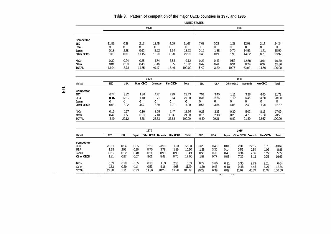
Table 3. Pattern of competition of the major OECD countries in 1970 and 1985 UNITED STATES

1970 1985

Competitor EEC USA Japan Other OECD

NlCs Other TOTAL

1970

Market EEC USA OtherOECD Domestic Non-OECD Total

Competitor EEC 6.74 3.32 1.30 4.77 7.29 23.43 USA 0.45 12.12 1.18 9.71 3.84 27.30 Japan 0 0 0 0 0 0 Other OECD 0.63 3.92 4.07 3.89 1.70 14.20

NlCs 0.19 1.17 0.10 3.05 9.47 13.99 Other 0.47 1.59 0.23 7.40 11.39 21.08 ~

TOTAL 8.49 22.12 6.88 28.83 33.68 100.00

A

P

11.59 0.38 2.17 13.45 4.09 0 0 0 0 0 0.18 2.28 0.62 8.62 1.54 1.03 0.31 11.15 15.90 0.90

0.30 0.24 0.25 4.74 3.58 0.84 0.58 0.46 6.46 8.35

13.94 3.78 14.65 49.17 18.46

1985

EEC USA Other OECD Domestic Non-OECD Total

7.59 3.40 1.11 3.28 6.40 21.79 0.37 16.56 1.10 6.46 3.50 28.00 0 0 0 0 0 0 0.57 3.84 4.05 2.40 1.70 12.57

0.26 3.33 0.30 5.02 8.18 17.09 4.73 12.88 20.56 0.51 2.18 0.26

9.30 29.31 6.82 21.89 32.67 100.00

31.67 0

13.23 29.28

9.12 16.70

100.00

1970

Market EEC USA Japan OtherOECD Domestic Non-OECD Total

7.08 0.28 1.28 0 0 0 0.19 1.88 0.70 0.46 0.21 1.93

0.23 0.43 0.52 0.47 0.41 0.34 a42 3.20 10.76

1985

EEC USA Japan Other OECD Domestic Non-OECD Total

12.93

14.51 14.62

12.68 8.29

63.03

0

NlCs 0.53 0.29 0.05 0.18 1.89 2.58 5.53 Other 1.63 0.39 0.18 0.53 4.16 4.65 11.49 TOTAL 29.30 5.71 0.93 11.86 40.23 11.96 100.00

2.17 24.34 0 0 1.71 18.99 0.70 23.92

3.04 16.89 6.37 15.86

14.59 100.00

0.77 0.66 0.11 0.30 2.79 2.01 6.64 1.79 0.43 0.10 0.48 4.46 5.27 12.54

29.29 6.39 0.89 11.07 40.39 11.97 100.00

competitor EEC 23.29 0.54 0.05 2.23 23.99 1.90 52.00 USA 1.68 2.99 0.16 0.70 3.78 1.19 10.50 Japan 0.36 0.52 0.48 0.21 0.98 0.93 3.49 Other OECD 1.81 0.97 0.07 8.01 5.43 0.70 17.00

23.29 0.46 0.04 2.00 22.12 1.70 49.62 1.28 3.30 0.14 0.56 2.54 1.02 8.85 0.58 0.76 0.46 0.34 2.36 1.22 5.72 1.57 0.77 0.05 7.39 8.11 0.75 16.63

FRANCE

NlCs 0.66 0.15 0.02 0.07 0.98 1.67 3.54 Other 1.62 0.21 0.06 0.18 4.96 7.16 14.18 TOTAL 29.92 3.11 0.45 5.12 46.68 14.73 100.00

1970 I 1985

0.79 0.49 0.08 0.13 2.09 1.63 5.21 1.59 0.32 0.07 0.18 5.23 6.87 14.27

26.84 4.81 0.67 5.14 48.36 14.18 100.00

Market EEC USA Japan Other OECD Domestic Non-OECD Total I EEC USA Japan Other OECD Domestic Non-OECD Total I

1970 EEC USA Japan OtherOECD Domestic Non-OECD Total

Competitor EEC 23.67 0.39 0.03 1.38 37.11 2.59 60.16 USA 1.64 1.58 0.08 0.40 4.34 1.58 9.61 Japan 0.39 0.28 0.23 0.09 0.41 0.98 2.38 Other OECD 1.94 0.51 0.03 3.00 3.88 0.76 10.13

1985 EEC USA Japan Other OECD Domestic Non-OECD Total

21.16 0.43 0.04 1.32 33.48 2.24 58.77 1.10 2.44 0.10 0.37 2.90 1.30 8.20 0.61 0.56 0.34 0.16 1.20 1.37 4.24 1.60 0.57 0.04 2.98 3.46 0.77 9.42

1970 1985

Market

Competitor EEC

-. USA VI Q, Japan

Other OECD

NlCs Other TOTAL

22.45 0.70 0.04 1.64 27.67 2.66 55.16 1.46 2.99 0.09 0.47 4.58 1.33 10.92 0.36 0.52 0.27 0.11 0.76 1.03 3.07 1.79 0.97 0.04 3.50 5.19 0.81 12.29

0.54 0.29 0.03 0.08 2.22 2.60 5.75 1.53 0.39 0.07 0.22 4.86 5.73 12.81

28.14 5.86 0.53 6.02 45.29 14.16 100.00

21.81 0.62 0.04 1.71 25.48 2.51 52.17 1.03 3.64 0.10 0.47 2.48 1.32 9.03 0.64 0.84 0.34 0.22 0.82 1.52 4.38 1.57 0.84 0.04 3.82 4.39 0.84 11.49

0.76 0.73 0.08 0.17 2.83 2.07 6.64 1.50 0.48 0.07 0.25 6.84 7.16 16.30

27.31 7.15 0.68 6.63 42.83 15.40 100.00


NlCs 0.29 0.31 0.05 0.19 2.82 3.52 7.17 Other 0.77 0.42 0.13 0.51 8.26 7.38 17.46 TOTAL 17.40 6.15 0.97 12.30 45.02 18.16 100.00

16.98 0.55 0.05 1.29 27.95 2.07 48.88 0.89 3.28 0.11 0.57 5.74 1.19 11.78 0.43 0.75 0.37 0.30 2.88 1.40 6.14 1.10 0.76 0.04 3.78 6.60 0.66 12.94

0.53 0.66 0.09 0.19 3.16 2.05 6.68 1.08 0.43 0.08 0.25 5.98 5.76 13.59

21.01 6.43 0.74 6.37 52.31 13.14 100.00

Table 3'(mnt). Pattern of competition of the major OECD countries in 1970 and 1985

CANADA

1970 Market EEC USA Japan OtherOECD Domestic Non-OECD Total


NlCs 0.20 1.21 0.06 0.81 1.59 0.16 4.44 Other 0.57 2.98 0.17 0.06 1.65 1.87 7.29 TOTAL 7.70 39.30 1.29 1.43 45.57 4.72 100.00

~~ ~

1985 EEC USA Japan OtherOECD Domestic Non-OECO Total

2.07 5.19 0.10 0.17 5.39 0.66 13.56 0.11 25.28 0.19 0.06 31.11 0.37 57.11 0.06 5.82 0.64 0.07 3.70 0.40 10.68 0.13 0.93 0.05 0.47 1.11 0.15 2.85

0.07 5.08 0.15 0.03 3.02 0.61 8.96 0.14 3.32 0.14 0.04 1.67 1.53 6.83 2.58 45.62 1.26 0.84 46.00 3.70 100.00

Notes The tables should be interpreted as follows: For the United States, in 1985, domestic market competitiveness represented 63.03 per cent of overall competitiveness, and the market share of the EEC In the home market was 20.51 per cent (12.93/63.03); the overall weight of the EEC in all markets combined was 24.34 per cent In these tables, the NlCs are as specfied in the OECD definition (see Note 3). The weight assigned to the home market is that of imports.

3. Accounting for the ne wly-industrializing countries in determining competitiveness

One factor that can alter a measure of competitiveness is the number of countries used to construct an indicator. As pointed out above, the last few years have witnessed the emergence of competition from the newly-industrializing countries, particularly those of South-East Asia (Taiwan, South Korea, Hong Kong and Singapore). In this section we set out to examine how these countries affect the measure of competitiveness. A particular feature of competition from the Asian countries is that it operates mainly on the American market which, in 1986, imported 67 per cent of total exports of manufactures from this area to the seven major OECD countries.

Chart A shows how the competitive position of the United States has altered since 1978, taking account of the trade performance of the dynamic East Asian countries. The three curves trace the movement of the indicators of overall competitiveness for the United States relative i) to its OECD competitors alone, ii) to the NIC group alone, and iii) to both. Two interesting features emerge. First, it can clearly be seen that, from 1982 onwards, the relative competitiveness of the United

150

145

140

135

130

125

120

115

110

105

100

- -

-

- -

-

-

-

-

-

-

CHART A

DECOMPOSITION OF THE RELATIVE COMPETITIVENESS OF THE UNITED STATES Indices

1980 = 100

1 150 - - - - - - - - -

-

95 - -

90 I I I I I I I

1978 1979 1980 1981 1982 1983 1984 1985 1986

___..----- Vis-B-vis the NlCs ,.---

Vis-8-vis OECD

/----- /--- /--

----- --_____+. -*

145

140

135

130

125

120

115

110

105

100

95

90

167

CHART B

TRADE OF MANUFACTURES BETWEEN THE USA Billion dollars AND THE NlCs Billion dollars

10 10

5 5

0 0

-5 -5

-1 0 -1 0

-1 5 -1 5

-20 -20

-25 -25

-30 -30

-35 -35

-40 4

-45 -45

-50 -50 1978 1979 1980 1981 1982 1983 1984 1985 1986

States worsened appreciably faster against the NlCs than against its OECD competitors; in particular, there was no reversal of the trend in the competitive position of the United States relative to the Asian countries in 1986, when the competitive position of the United States vis-8-vis other OECD competitors strengthened appreciably. This deterioration in the relative competitiveness of American producers vis-84s South-East Asia since 1980 is probably a major explanatory factor in the growth of U.S. imports from that region, and hence in the worsening of the trade balance on industrial goods relative to these countries (Chart B). Second, the impact of the trend in US. competitiveness relative to the NlCs on the indicator of the overall competitive position of the United States is small (Chart A). When the newly-industrializing countries are included in the calculation of the indicator of relative U.S. competitiveness, the weight of the four South-East Asian countries in the weighting pattern determining the average price of the United States' competitors works out at 17 per cent. While the NlCs represent a major source of competition for the United States, their influence should nonetheless not be overstated, particularly in explaining the growing imbalance in U.S. trade in manufactures from 198 1 onwards.

168

4. Comparing the indicators of competitiveness constructed by the OECD and other institutions

The various technical factors illustrated in the preceding section enter, one way or another, into the indicators of competitiveness constructed by different institutions. These factors account for sometimes important divergences in the measures produced. In practice, there are two principal sources for divergence: the number of countries used in the calculations, and the weighting pattern adopted. The summary table (Table 4) is an attempt to pinpoint the main differences in approach and so place in context the indicators calculated by the OECD.

A few comments are perhaps called for as regards the weighting pattern used in constructing measures of competititveness:

- Many institutions use bilateral or multilateral export weighting patterns (described in Table 1). These systems are in fact special cases of the

Table 4. Elements of comparison of competitiveness indicators calculated by various organisations

Weighting system t::t: 9 Mathematical Trade matrix Fixed/current weights Organisation Variable calculated

cluded

OECD Effective exchange rate Double weighting based 23 Geometric 1970-1984 Current on supply

Relative export price 15 Relative unit labour cost 15 Relative consumer price 23

Relative export price of the Double weighting based 23 Geometric 1985 Fixed INTERLINK model' on exDorts

IMF Effective exchange rate MERM 17 Geometric Fixed

Morgan Effective exchange rate 1 Bilateral imports and ex- 16 Geometric Average for Fixed Guaranty Trust ports period

1980.87 Effective exchange rate 2 Double weighting based 41 Geometric idem Fixed

on imports and exports

US Federal Effective exchange rate Bilateral imports and ex- 10 Geometric Average for Fixed Reserve Board ports period

UK Treasury Effective exchange rate MERM 17 Geometric Fixed

1972-76

US Treasury Effective exchange rate Bilateral imports and ex- 44 Arithmetic Fixed

Banque Effective exchange rate Multilateral exports 13 Geometric 1970-78 Current de France**

pans

Relative export price Bilateral exports 16

** calculated but not published: for weighting matrix see Statistical Annex. calculated but not published: see Etienne eta/.. 1980.

169

OECD's double weighting system for export competitiveness described in Part I1 of this paper. If it is assumed, first, that on each of the markets a country's only competitors are domestic producers for that market and, second, that competitiveness between countries is determined only on their own markets, then the double weighting pattern boils down to a single weighting pattern based on bilateral exports. Admittedly, this system is highly rudimentary. It entirely ignores competition between the two countries on third markets. Alternatively, if one considers there to be only one market, namely the world market, and that on this market competition operates between exporters (excluding domestic producers), the double weighting pattern is simplified to a single multilateral weighting pattern involving only the relative weights of each country's exports in world trade.

- Similarly, weighting patterns for overall trade competitiveness based on bilateral imports and exports are special cases of the double weighting pattern used by the OECD. These patterns consist in calculating import-competitiveness and export-competitiveness separately, and then combining these measures either with equal weight, or with weights reflecting the ratio of imports to exports. Finally, indicators calculated on the basis of an MERM-type weighting are of the same type as the indicators used in the INTERLINK model. Both in effect derive from a macroeconomic model based on the same analytical framework. However, as mentioned earlier, MERM weights are obtained by "shocking" a model and observing the results on a specific variable (imports, exports or trade balance) for a country and its trading partners. It would seem a natural further development for the OECD to use an MERM "shocking procedure" to recover the weights implicit in INTERLINK and compare these with the weights in the published OECD competitiveness measures. This project is under way.

-

B. Comparative trends in the OECD's measures of competitivenes

Chart C shows, for each of the seven major OECD countries, the trend since 1970 in the indicators of import-, export- and overall competitiveness described in Part 11. Two measures of overall competitiveness are given here - that of relative export prices and that of relative unit labour costs - in order to take into account, as mentioned in Part I, trends in relative profitability in manufacturing. It is not the place here to study in detail either the ultimate determinants of competitiveness or the impact of fluctuations in competitiveness on the major OECD countries' trade in

170

130 1

240

230

220

210

200

190

180

170

CHART C

INDICATORS OF RELATIVE COMPETITIVENESS Indices 1970 = 100

Global competitiveness Export and import competitiveness -----Relative export price United States ....... Relative export price -Relative unit labour cost - Relative import price

- 240

- 230 - - - 220

- - 210

- 200

- 190

- - 180

- 170 -

-

- -

4 130

120 - - 120

t i o - 4---.

- 90

70 71 12 73 74 75 76 77 70 79 00 01 02 03 04 05 86

150

120

130 1

Japan

240 240 - - 230 - 220 - 210 - 200 - 190 - 180 - 170 - 160 - 150 - - 150

- 140

- 130

- 120

110 -

90 - 90

80 80 I 1 1 ' I I I I I I I I 1 1 I I 70 71 12 73 74 76 78 77 i a 79 00 01 a2 03 M a6 08

-

Germany

150 1;:

171

Z L 1

011

011

OEl

- -

- OEL

0 1

- -

-

98 58 b8 E8 18 I 8 08 6L 8L LL 91 5L bL C l ZL I L OL 98 58 b8 E8 18 18 08 6L 8L LL 9L 5L bL EL ZL I L OL OL OL OL

- 08 l I I I I I , I I , I I I I - I I I I I I I I I I I I I I OL

- 06 06

001 001

011 011

021 O Z I

- -

- - 011

O Z I O Z I

OEL O E I O E I OEI - - O t l - -RL R1- O t l

- - - - - - - -

BpBUB3

- - 011

- - OZt

- OEL

- - or1

-

98 58 b8 E8 28 18 08 6L 8L LL 9L 5L bL EL ZL 1L OL 08

05 .,t L

98 58 b8 E8 18 I 8 08 6L 8L LL 9L 5L bL EL ZL 1L OL 08 08 ( 1 1 1 1 1 1 1 1 1 1 1 1 1 1 1 06 -

- OZL

O E I

II

051 - 051 - - -

manufactures. Nonetheless, examination of these curves does reveal a number of salient features demonstrating the relevance of the indicators calculated:

- The overall competitiveness of the three main countries (United States, Japan and Germany) is strongly influenced by movements in the dollar exchange rate. Thus, the declines in the U.S. exchange rate from 1970 to 1973, and again from 1976 to 1978, correspond to periods of loss of relative competitiveness for Japan and Germany. Similarly, the appreciation of the U.S. real effective exchange rate from 1974 to 1976 led to an improvement in the competitive positions of these countries. On the other hand, the various EMS realignments which, admittedly, were not so far-reaching did not result in any sizeable changes in the relative competitiveness of the main European countries (France, Italy and Germany). It is remarkable, for instance, how little France's competitive position since 1975 - particularly its import-competitiveness - has been affected by the franc's successive devaluations relative to the other European currencies. These devaluations of the franc seem to have moderated potential losses in French competitiveness rather than to have contributed to the improvement of France's competitive position. Despite the major fluctuations in the yen exchange rate since 1970, Japan's relative export-competitiveness has, as measured by export unit values, remained relatively stable over the whole of the period, The fact that Japanese relative export prices have shown little movement may in part be explained by the trend in Japanese exporters' profit margins. Chart D compares, for Japan and the United States, the ratio of export price indices for manufactures to industrial unit labour costs. The trend in this ratio shows, in particular, how American and Japanese export margins have performed over the period'O. It emerges that while, by and large, Japanese exporters have pursued a policy of squeezing (increasing) their margins whenever their export-competitiveness was declining (improving), U.S. exporters generally set their prices with primary regard to production costs, even when the dollar was appreciating steeply between 198 1 and 1985. Competitors' prices appeared to have relatively little weight in price-setting by U.S. exporters.

- A comparison of trends in export- and import-competitiveness in France and Italy is also revealing, with the former converging and the latter diverging. While the structure of competition is very similar in France and Italy (see Part 111. A.2), a comparison of the respective trends in the volume of their foreign trade in manufactures shows that Italy has considerably

-

173

CHART D

EXPORT PRICE - UNIT LABOUR COSTS RATIO Comparison USA - Japan

145

140

135

130

1.25

120

115

110

- - 145 140 ___.---- -

- United States ..----__._I__--- .** - 135 - 130

- 125 - 120

- 115

- -

/-. ,,..-- -

.' ,.---- ..--. ** ,.*' -.-.-------......' , I ,#-- -

- - ,/' - 110

145

140

135

130

1.25

120

115

110

CHART E

Indices IMPORT COMPETITIVENSSS:

Indices 1970= 100 Comparison Italy - France 1970= 100

150 150 - 145 - 140 - 135 -

130 130 - 125 125

120 120

- 115

-

-

- - - -

- 105 1w

95 95

9 0 - 90

I I I I I I 1 I I I l l I I l l 85 85 1970 1971 1972 1973 1974 1975 1976 1977 1978 1979 1980 1981 1982 1983 1984 1985 1986

- - - -

- - 145 140 ___.---- -

- United States ..----__._I__--- .** - 135 - 130

- 125 - 120

- 115

- -

/-. ,,..-- -

.' ,.---- ..--. ** ,.*' -.-.-------......' , I ,#-- -

- - ,/' - 110

174

Table 5. Growth of export and import volumes of manufactures for France and Italy

1970/86 1970174 1974180 1980185

Exports1 France Italy

Imports’ France Italy

5.3 5.4

11.3 7.3

5.6 1.5 5.7 4.5

8.1 13.0 8.7 3.2 5.4 6.7 7.3 2.0

Balance2 France -11.8 -0.3 -4.6 -3.1 Italy 4.6 1.3 0.5 3.4

~~~

1. Average annual growth rates. 2. Differential in 1970 US$ billion.

outperformed France between 1970 and 1986 (Table 5). While, on balance, between 1970 and 1986 Italian and French exports displayed fairly similar rates of growth, import volumes increased much less rapidly in Italy than in France. One reason for this would seem to have been the much greater deterioration in France’s import-competitiveness (Chart E), which would in large measure explain the difference in the two countries’ foreign trade performance over the period 1970- 1986 with respect to manufactures. Since 1980, the faster rise of Italian exports relative to French exports, particularly to OECD markets, has also served to widen the differential between the two countries’ external balances on trade in manufactures.

CONCLUSION

The methodological problems involved in constructing indicators of competitiveness have been set out in detail in this paper. We have attempted to show that there is no single perfect measure. The construction of indicators hinges on what aspect of competition it is sought to study. Thus, various measures of import-, export- or overall competitiveness have been identified, together with their respective fields of application. Furthermore, for one and the same definition, a number of different measures of competitiveness may be advanced. Their quality

175

depends on the components used to construct them, the geographical coverage and the level of aggregation of markets and competitors.

Despite the serious problems posed by construction and aggregation, indicators of competitiveness can be a useful analytical tool. The measures calculated by the OECD, by breaking down and analyzing changes in the major countries' exposure to competition, have helped, for instance, to reassess the importance of the newly-industrializing countries of South-East Asia as competitors on the world market. Moreover, for a number of countries, long-term movements in the OECD's indicators of competitiveness shed light on trends in trade volumes, both directly by pinpointing causes for demand shifts, and indirectly by indicating changing patterns of profitability in the tradeable goods sectors.

TECHNICAL ANNEX

Price-competitiveness measured by a real effective exchange rate

The price differential used to measure the competitiveness of a country; is normally written:

/nCi = Inpi- 2 Idwy . Pj) j # i

where

and (w,j) the weighting pattern

Pi is the dollar price (or cost) index of country i

In fact, the dollar indices may be broken down into

Pi = PI, . E;

where PI, is the price expressed in the currency of country i and Ei the exchange rate against the dollar. The expression may hence be written:

lnC; =

= [In P l i - j s i wb . In Plj] + [In E,- 2 wu. In 51 In (PI; . Ei) - 2 wu . In (Plj . Ej)

j # i

j # i

E;/ X wjj.6 j # i

and therefore Ci = x PljWy/Pl; j # i

which is by definition the real effective exchange rate of country iwhen PI is adopted as the deflator.

176

Table A l . Weighting matrix (29x29) 1985: Export competitiveness defined in INTERLINK

USA CAN JAP FRA GER ITA UKM BLX NET IRE GRE DEN NOR SWE FIN

USA CAN JAP FRA GER ITA UKM BLX NET IRE GRE DEN NOR SWE FIN ICE OST SWI SPA POR TUR ASL NZD LOP HOP OOP NIC LMI sov

-.A

4 4

0 2.17

14.38 12.09 12.11 11.07 12.59 10.21 10.04 11.05 10.65 9.94

10.82 9.96 8.57

10.29 9.37

11 .08 11.51 8.96

10.65 18.42 20.83 14.58 13.85 7.78

11.16 12.51 14.10

1.03 0

10.58 2.61 3.01 3.06 3.72 1.97 1.97 2.78 1.84 2.57 2.29 3.19 1.82 2.35 1.45 2.64 2.54 2.51 1.52 3.09 4.12 2.32 5.58

12.29 11.79 5.79 2.01

20.61 30.18 0

13.11 12.56 13.31 14.85 9.79 9.92 9.55

11.68 1 1.85' 12.42 11.85 10.62 8.29

10.26 12.23 12.39 9.61

13.13 20.09 20.04 13.33 16.28 21 .80 21.92 16.09 16.85

7.60 14.63 6.57 7.83 3.32 2.96 0.72 0.22 0.86 0.71 2.43 0.85 4.02 9.61 4.39 5.33 1.65 1.49 0.40 0.09 0.54 0.37 1.72 0.43 6.60 12.66 6.23 7.13 2.67 2.43 0.45 0.20 0.83 0.68 2.07 0.79 0 17.65 7.01 7.23 4.42 4.89 0.79 0.32 1.02 0.82 2.54 1.10 9.60 0 9.08 8.31 6.12 5.00 0.98 0.26 1.26 0.98 3.43 1.65 7.52 17.39 0 6.95 5.31 4.55 0.76 0.31 0.96 0.72 2.43 1.15 7.69 16.49 6.85 0 4.35 3.89 0.53 0.26 1.13 0.79 2.63 1.05 7.83 19.59 8.75 7.32 0 4.51 0.99 0.33 1.09 0.89 2.70 1.13 9.65 17.83 8.30 7.19 4.97 0 0.95 0.32 1.13 0.86 3.02 1.17 7.97 18.10 7.10 4.99 5.52 4.81 0 0.24 1.15 0.95 2.91 1.20 8.85 13.11 8.00 6.86 5.08 4.55 0.67 0 0.92 0.73 2.27 1.05 7.17 16.48 6.27 7.23 4.26 4.02 0.80 0.23 0 1.38 4.54 2.26

3.07 1.95 7.47 16.54 6.10 6.71 4.49 3.96 0.85 0.24 1.79 0 7.22 18.28 6.42 7.08 4.29 4.39 0.82 0.23 2.00 0.99 0 1.58 7.07 19.53 6.84 6.18 4.01 3.75 0.74 0.24 2.02 1.36 3.29 0 8.82 18.14 7.51 5.72 4.26 4.53 0.88 0.24 1.10 0.77 3.29 1.43 9.64 14.72 8.51 6.89 5.31 5.02 0.72 0.39 1.10 0.82 2.71 1.90 7.89 15.74 7.53 6.43 4.94 4.36 0.76 0.32 0.99 0.79 2.50 1.16 7.33 16.92 7.51 6.52 5.02 3.87 0.70 0.28 0.87 0.70 2.14 1.02 7.66 18.15 7.61 6.44 5.68 4.66 1.01 0.26 1.36 1.02 3.22 1.36

10.29 13.10 8.23 6.89 4.27 4.10 0.67 0.36 0.85 0.63 2.01 0.86 5.58 10.02 4.43 6.09 2.21 2.09 0.53 0.13 0.75 0.68 1.51 0.61 3.94 8.94 3.75 6.05 1.49 1.40 0.49 0.08 0.54 0.45 1.68 0.57 9.14 14.84 5.82 5.63 3.06 2.99 0.64 0.23 0.71 0.60 1.79 0.61 5.70 11.79 5.05 5.06 2.83 2.38 0.49 0.17 0.69 0.61 1.66 1.05 4.45 10.05 4.75 5.04 2.24 2.05 0.44 0.13 0.55 0.41 1.62 0.56 5.96 12.04 5.62 5.81 2.69 2.42 0.53 0.19 0.76 0.57 2.00 1.05 5.98 13.93 6.08 5.83 3.43 3.19 0.57 0.19 0.64 0.51 1.89 0.93 7.88 13.86 6.40 6.56 3.70 3.38 0.50 0.27 1.06 0.93 2.37 0.78

Table A 1 (cont.). Weighting matrix (29x29) 1985: Export competitiveness defined in INTERLINK

USA CAN JAP FRA GER ITA UKM 8LX NET IRE GRE DEN NOR SWE FIN

~ ICE 03 OST

SWI SPA POR TUR ASL NZD LOP HOP OOP NIC LMI sov

A

ICE OST SWI SPA POR TUR ASL NZD LOP HOP OOP NIC LMI SOV

0.02 1.25 2.62 1.85 0.33 0.43 0.63 0.30 0.35 0.57 1.79 12.99 3.85 2.68 100 0.01 0.47 1.48 0.96 0.24 0.16 0.24 0.13 0.13 0.52 4.85 23.50 4.02 0.90 100 0.01 1.08 2.31 1.58 0.30 0.45 0.57 0.23 0.26 0.54 3.00 15.41 3.87 2.71 100 0.02 2.16 3.00 1.91 0.50 0.76 0.30 0.08 0.37 0.36 1.15 8.52 2.78 2.48 100 0.02 1.81 3.43 2.36 0.66 0.51 0.26 0.09 0.31 0.38 1.31 8.73 3.38 2.40 100 0.02 2.05 3.08 2.11 0.54 0.65 0.25 0.08 0.25 0.34 1.33 8.58 3.04 2.18 100 0.01 1.62 2.58 1.80 0.45 0.53 0.34 0.14 0.24 0.33 1.39 8.70 2.85 2.19 100 0.02 2.11 3.34 2.34 0.67 0.56 0.21 0.06 0.22 0.32 1.06 7.05 2.86 2.10 100 0.02 2.22 3.26 1.98 0.60 0.60 0.22 0.06 0.24 0.30 1.07 7.02 2.96 2.13 100 0.02 1.61 2.90 1.82 0.66 0.50 0.29 0.11 0.26 0.31 1.18 7.73 2.67 1.61 100 0.02 2.38 3.32 2.05 0.48 0.75 0.21 0.05 0.26 0.31 1.01 7.99 2.55 2.37 100 0.02 1.71 2.62 1.57 0.62 0.43 0.28 0.08 0.20 0.30 1.01 7.71 2.08 2.35 100 0.02 1.65 2.70 1.65 0.60 0.42 0.34 0.09 0.22 0.35 0.98 7.50 2.16 2.66 100 0.02 1.73 2.69 1.56 0.62 0.41 0.22 0.10 0.20 0.29 1.18 8.04 2.45 2.18 100 0.02 2.70 2.79 1.68 0.56 0.40 0.21 0.08 0.15 0.43 0.95 9.67 2.77 1.54 100 0 2.39 2.49 1.43 0.57 0.39 0.28 0.10 0.27 0.42 1.08 8.51 2.80 1.64 100 0.03 0 3.40 1.85 0.54 0.74 0.20 0.05 0.25 0.35 0.96 7.90 2.89 2.04 100 0.02 2.00 0 1.85 0.50 0.58 0.29 0.10 0.24 0.38 1.25 8.22 3.05 2.17 100 0.01 1.59 2.72 0 0.47 0.56 0.29 0.08 0.29 0.34 1.12 8.13 2.71 2.37 100 0.02 1.83 2.91 1.87 0 0.46 0.21 0.05 0.21 0.29 1.07 7.13 2.45 1.99 100 0.01 2.23 2.95 2.00 0.40 0 0.27 0.04 0.71 0.20 0.93 7.45 2.77 2.47 100 0.01 0.80 2.02 1.35 0.25 0.36 0 0.21 0.36 0.63 1.36 10.00 3.72 2.72 100 0.01 0.55 1.74 0.88 0.15 0.13 0.52 0 0.25 0.62 1.52 13.49 4.22 1.54 100 0.02 1.38 2.23 1.85 0.34 1.27 0.49 0.14 0 0.42 1.06 8.89 3.03 2.61 100 0.02 1.23 2.27 1.38 0.29 0.24 0.55 0.22 0.27 0 1.93 12.58 3.77 2.06 100 0.01 0.80 1.78 1.09 0.26 0.26 0.28 0.13 0.16 0.46 0 15.91 3.50 1.19 100 0.01 1.19 2.16 1.44 0.31 0.36 0.39 0.22 0.25 0.58 3.12 0 3.79 1.67 100 0.01 1.37 2.49 1.50 0.34 0.43 0.44 0.20 0.27 0.52 2.00 11.24 0 1.60 100 0.01 1.43 2.58 1.94 0.41 0.57 0.48 0.11 0.33 0.41 1.00 7.76 2.32 0 100

CAN USA JAP ASL OST BLX DEN FIN FRA GER ITA NET NOR SWE SWI

4 UKM 4 (D

Table A2. Weighting matrix (16x16) 1985: Overall trade competitiveness

CAN USA JAP ASL OST BLX DEN FIN FRA GER

0 77.50 8.50 0.32 0.26 0.61 0.27 0.25 1.99 3.44 29.52 0 34.62 0.71 0.46 1.63 0.84 0.45 4.71 10.23 5.62 54.66 0 5.20 0.68 1.22 1.65 0.65 4.65 10.16 2.68 28.35 32.72 0 0.48 1.04 0.68 0.84 3.36 9.41 0.46 4.60 4.33 0.22 0 2.81 0.89 1.13 5.57 51.78 0.85 10.24 4.54 0.35 1.16 0 0.93 0.73 18.40 25.49 0.70 7.54 6.97 0.39 1.35 3.46 0 3.61 6.12 25.26 0.65 5.96 7.16 0.39 2.27 2.97 4.15 0 6.37 23.88 0.84 9.96 4.69 0.48 1.17 12.22 1.00 0.88 0 29.11 0.92 11.00 7.87 0.51 5.51 8.75 2.13 1.53 14.73 0 0.95 11.38 4.68 0.74 3.26 5.51 1.29 0.77 20.00 29.18 1.03 11.48 5.46 0.43 1.13 12.99 1.32 1.01 10.54 31.13 0.68 7.62 6.83 0.37 1.37 2.94 8.34 4.30 5.37 18.79 1.13 11.24 5.99 0.59 1.58 3.55 8.07 7.66 7.37 21.86 0.78 8.96 6.26 0.37 4.49 4.19 1.08 0.87 13.54 33.97 1.9 16.51 8.22 1.06 1.26 6.74 2.63 2.08 11.54 22.19

ITA NET NOR SWE SWI UKM

1.81 0.68 0.14 0.87 0.58 2.80 5.28 1.74 0.41 1.91 1.52 5.97 3.71 1.44 0.73 1.51 3.13 4.98 4.88 1.64 0.32 2.44 1.53 9.62 11.04 3.39 0.53 2.23 6.80 4.23 6.69 15.33 0.62 2.39 2.09 10.17 5.20 5.84 5.09 15.46 2.55 10.46

15.79 7.65 0.58 2.20 3.66 9.77 12.41 14.13 1.21 3.60 5.73 9.98 0 6.01 0.63 2.26 4.60 8.73 6.28 0 1.12 2.63 1.92 11.54 4.15 4.82 0 21.53 2.02 10.87 4.75 4.78 6.67 0 2.58 12.17 11.76 3.85 0.63 2.28 0 6.96 8.41 8.41 1.68 4.43 2.94 0

5.75 4.52 3.21 19.32 2.88 10.51

- 100 100 100 100 100 100 100 100 100 100 100 100 100 100 100 100

NOTES

1.

2. 3.

4.

5.

6.

7.

8.

9.

10.

The studies by T.P. Hill (see OECD Economic Studies No. 61, which have recently been updated (see article by D. Blades and D. Roberts in this issue), attempt to measure internationally comparable absolute price levels, based on purchasing power parities. Unfortunately, from the perspective of competitiveness analysis, these measures pertain to the purchase prices of the full range of goods entering into domestic expenditures, including non-tradeable goods, and also including consumption taxes. These measures are thus of only limited use for the narrower purpose of assessing relative consumer price levels among OECD countries.

See R. Herd, 1987.

The NICs, as defined by the OECD, are Argentina, Brazil, Hongkong, Israel, the Philippines, Singapore, South Africa, South Korea, Taiwan, Thailand and Yugoslavia.

For the breakdown of non-OECD countries into these six groupings, see OECD Economic Outlook, "Sources and Methods".

Only the following sixteen countries for which homogeneous cost data are available are included in the calculations: United States, Japan, Germany, France, United Kingdom, Italy, Canada, Australia, Austria, Belgium, Denmark, Finland, Netherlands, Norway, Sweden and Switzerland.

The equations are specified in terms of changes in competitiveness and the resulting indicators are thus expressed in terms of price changes. The prices given here are hence expressed as growth rates, as indeed they are hereafter. This implies that the weighted average is a geometric average. Relative to the other options (arithmetic, harmonic, etc), the latter is the only one that provides a certain number of basic properties (for more details, see Pincon, 1979).

These indicators are published twice yearly in OECD Economic Outlook and monthly in Main Economic Indicators.

See Artus and Rhomberg (1 973).

Home markets are taken into account with an equal weighting to that of imports.

The ratio of export prices to unit costs comprises two elements: the ratio of producer prices to unit costs, and the ratio of export prices to producer prices. It thus reflects two margins, that on the home market and and that on expQrt markets.

180

BIBLIOGRAPHY

Armington P. (1 969), "A theory of demand for products distinguished by place of production",

Armington P. (1 969a), "The geographic pattern of trade and the effects of price changes",

Artus J. and R. Rhomberg (1 973), "A multilateral exchange rate model"; lnternational Monetary

Bank of England (1 982), "Measures of competitiveness", Quarterly Bulletin (September),

Belongia M. (1 986). "Estimating exchange rate effects on exports: a cautionary note", federal

Debonneuil M. and M. Delattre (1 987), "Le commerce extkrieur de la France: une thkorie pour la

lnternational Monetary fund Staff Papers (March), pp. 159-1 75.

lnternational Monetary fund Staff Papers (July), pp. 1 79-1 99.

fund Staff Papers (November), pp. 591 -61 1.

pp. 369-375.

Reserve Bank of Saint-Louis (January), pp. 5-1 6.

pratique", lNSEE (March).

Durand M. (I 986), "Method of calculating effective exchange rates and indicators of competitiveness", OECD Department of Economics and Statistics Working Paper No. 29, (Febru- ary).

Economie Europhenne (1 9851, (September) No. 25. Etienne, Pincon, Farkas and Laclaire (1980). "Une mkthode de mesure de la compktitivite

internationale des produits francais", Bulletin Trimestriel de /a Banque de France (March),

Federal Reserve Board (1 985), "Index of the weighted average exchange value of the U.S. dollar:

Federal Reserve Board (1 987), "Measuring the foreign-exchange value of the dollar", Bulletin

pp. 19-31.

revision", Bulletin (November), pp. 700-701.

(June), pp. 41 1-422. Feldstein M. and P. Baccheta (1 987). "How far has the dollar fallen?", National Bureau of

Economic Research Working Paper 2 1 22 (January).

Herd, R. (1 987). "Import and export price equations for manufactures", OECD Department of

Hickman B. and Lau L. (1 973). "Elasticities of substitution and export demands in a world trade

Hirsch F. and Higgins I. (1 970). "An indicator of effective exchange rates", lnternational Monetary

Economics and statistics Working Paper No. 43. (June).

model:, European Economic Review (December), pp. 350-380.

fund Staff Papers (November), pp. 453-487.

181

H.M. Treasury (1 977), 'The effective exchange rate for sterling", Economics Progress Report

H.M. Treasury (1 981), "The effective exchange rate for sterling", Economics Progress Report

H.M. Treasury (1 984). "Sterling exchange rate index", Economic Progress Report (October),

Maciejewski E. (1 983), 'Real effective exchange rate indices. A re-examination of the major conceptual and methodological issues", lnternational Monetary Fund Staff Paper (Septem- ber), pp. 491-541.

Morgan Guaranty Trust (1 983). "Effective exchange rates: update and refinement, World Financial Markers (August), pp. 6-1 4.

Morgan Guaranty Trust (1 986), "Dollar index confusion", World Financial Markets (October- November), pp. 14-1 7.

OECD (1 978), "The international competitiveness of selected OECD countries", Occasional Studies (July), pp. 35-50.

Pincon R. (1 979), "R6flexions rnbthodologiques concernant les calculs de taux de change ponderes et d'indices de cornQ6titivit6". CaAiers Bconomiques et monhtaires de /a Banque de France (February), pp. 89-1 07.

Rhomberg R. (1 976), "Indices of effective exchange rates". International Monetary Fund Staff Papers (March), pp. 89-1 12.

(March), pp. 1-3.

(February), p. 7.

pp. 1-2.

182

A NOTE ON THE NEW OECD BENCHMARK PURCHASING POWER PARITIES FOR 1985

Derek Blades and David Roberts

CONTENTS

Introduction . . . . . . . . . . . . . . . . . . . . . . . . . . . . . . . . 184

I. Using PPPs . . . . . . . . . . . . . . . . . . . . . . . . . . . . . 184

II. Calculating PPPs . . . . . . . . . . . . . . . . . . . . . . . . . . 186

111. Results for 1985 . . . . . . . . . . . . . . . . . . . . . . , . . . 187

IV. Comparison of the 1980 and 1985 PPPs . . . . . . . . . . . . . 190

V. Extrapolations for 1986 and 1987 . . . . . . . . . . . . . . . . . 192

VI. Future work on PPPs . . . . . . . . . . . . . . . . . . . . . . , . 194

Bibliography . . . . . . . . . . . . . . . . . . . . . . . . . . . . . . . 196

The authors are Principal Administrators in the Economic Statistics and National Accounts Division. They wish to acknowledge the helpful comments of Peter Hill and Michgle Hainaut, and to thank loanna Alexopoulou for preparing the tables.

183

INTRODUCTION

Two years ago, the OECD released a set of Purchasing Power Parities (PPPs) for eighteen OECD countries based on price and expenditure data for 1980. Some of the main results were published in OECD Economic Studies, No. 6 (Hill, 19861, and in the 1986 edition of National Accounts, Vol. 1 (OECD, 19861, and a detailed description of the methods and results of these 1980 benchmark PPPs is given in Ward ( 1985). The 1980 PPPs were calculated jointly by the Statistical Office of the European Communities (EUROSTAT) and the Economic Statistics and National Accounts Division of the OECD Economics and Statistics Department. A new set of benchmark PPPs is now available for twenty-two OECD countries based on price and expenditure data for 1985. These PPPs were again calculated in collaboration with EUROSTAT, which collected price and expenditure data for its own Member countries, while the OECD arranged for comparable data to be provided by the non-EEC members of OECD'.

The main purpose of this note is to present these new PPPs based on 1985 and to explain how they differ from the 1980 benchmark estimates. First, however, there is a brief discussion of some of the uses that can be made of PPPs, followed by a short description of how they have been calculated. A final section gives some estimates for 1986 and 1987.

1. USING PPPs

As their name implies, Purchasing Power Parities are the rates of currency conversion that equalize the purchasing power of different currencies; thus, $100 converted into Yen at the PPP 'rate of exchange" will buy the same basket of goods and services in Japan as in the United States. The PPPs discussed here have been calculated using, as weights, final expenditures on the GDP, and so they can be used

184

- and this is their main purpose - to make inter-country comparisons of GDP and its expenditure components in real terms. When the GDPs of two countries are converted into a common currency using PPPs, comparisons can be described as being in "real terms" in the same way that changes in a country's GDP over time are measured in "real terms" by revaluing current GDP using the constant prices of some base year.

Much of the OECD's analytic work involves comparisons of economic aggregates between Member countries, and the ability to make such comparisons in real terms is in itself a sufficient justification for the time and expense devoted to the calculation of PPPs. In addition, however, PPPs and the price data underlying their calculation offer other interesting possibilities for economic and statistical research. It has long been known, for example, that the relative prices of goods and services vary in a consistent way with the level of GDP; Hill ( 1986) used the 1980 PPP results to examine this phenomenon in a previous issue of Economic Studies. The PPPs for the expenditure components of GDP show striking inter-country differences in the relative prices of capital versus consumer goods and of government versus private consumption (Ward, 1985); these differences clearly have implications - hitherto little explored - for studies of, respectively, capital productivity and the growth of the public sector. The comparison of successive benchmark estimates of PPPs provides an independent check on the reliability of the price and quantity indices used in the national accounts, since the change in a country's PPP-converted GDP between two successive benchmark years (such as 1980 and 1985) should be close to the real growth rate recorded in that country's national accounts estimates. The fact that there are frequently significant differences suggests that some countries' estimates of real growth and price inflation may be subject to substantial errors; the Economics and Statistics Department expects to investigate this question in the near future.

A final word should be added on a use for which the PPPs presented here are not relevant, namely for forecasting movements in exchange rates. This may seem odd since the concept of purchasing power parity was originally developed by Cassel (1916) in his work on "equilibrium" exchange rates, i.e. "underlying" rates of exchange towards which actual exchange rates are assumed to converge in the long term. To serve as a plausible candidate for an equilibrium exchange rate, a PPP would have to refer to domestic production of tradeable goods and services valued a t export prices. By contrast, the PPPs presented here refer to final expenditures, including non-tradeables such as government services and construction, valued at domestic market prices, including sales taxes. However, while the PPPs presented here are not appropriate for explaining or predicting exchange rates, the relationship between them is of considerable interest. The ratios of exchange rates to PPPs can

185

be interpreted as spatial price indices which quantify the differences in price levels between countries in the same way that temporal price indices measure changes in price levels over time.

II. CALCULATING PPPs

PPPs are calculated, like temporal price indices, from the relative prices of large numbers of carefully specified goods and services. For the 1985 PPPs, final expenditures on the GDP were first broken down into 239 categories referred to as "basic headings"2. These 239 categories represent the most detailed level for which the participating countries were required to supply expenditure weights. "Cheese", "dental services" and "single-family dwellings" are examples of basic headings. The next step was to identify a number of particular goods and services within each basic heading. A "250 gramme pack of Camembert cheese", an "extraction of a single-root tooth without complications" and a '5-room, detached, single-family house of 1 10 m2 habitable surface with a 21 m2 garage" are examples of the specific goods and services whose prices were used in calculating the 1985 PPPs.

The list of specific items was built up in consultation with statisticians from all the countries participating in the study so as to ensure that it contained a representative selection of the goods and services commonly found in each country. The items selected do not have to be available in all countries but they must obviously be available, and commonly purchased, in at least two. In total, some 3 600 specific items were defined3, and statistical agencies in the participating countries then arranged to supply the corresponding price data. To be consistent with the national accounts, these data refer to the average prices over the whole year and over the whole country, and they are market prices, i.e. they include consumption taxes.

For each basic heading, a matrix of size 22 x m is then constructed containing prices supplied by the 22 participating countries for the m items selected to represent that basic heading. This is then used to derive a matrix containing the 22 x 22 price ratios for the basic heading concerned. Almost invariably, there are two problems with this derived matrix. First, some of the price ratios are missing because, as already noted, not all 22 countries can supply prices for all the m items. Secondly, the ratios of the prices that are available are inconsistent between

186

countries in the sense that the price ratios between countries A and B and between countries A and C are not consistent with the price ratio obverved between countries C and 6: this is usually referred to as the problem of intransitivity. Price ratios are estimated for missing cells using the price ratios available for "bridge" countries, and the complete matrix is then made transitive by a process of geometric averaging referred to as the "EKS" method after the initials of its inventors4.

The EKS procedure generates a set of 22 transitive PPPs for each of the 239 basic headings and the next step is to aggregate these first to sub-groups such as "milk, cheese and eggs" and "residential buildings"; secondly to groups such as "food, beverages and tobacco" and "construction"; thirdly to the main components of final expenditure, such as "private consumption expenditure" and "gross fixed capital formation"; and finally to total GDP. Several weighting schemes have been suggested for this aggregation procedure, but the most widely-accepted, and the one currently used by EUROSTAT and the OECD, is the Geary-Khamis (GK) method which uses as weights the quantities consumed throughout the entire group of participating countries. An attractive feature of the GK method is that it treats countries as though they were regions of a single super-country, with the PPPs being obtained in the same way that national price indices would be obtained from regional indices compiled separately for large cities, small towns, rural areas, etc. An objection to the GK method is that it is in some sense "unfair" to small countries because the weights largely reflect the expenditure patterns of the bigger members of the group. Different weighting systems would of course produce different PPPs, but the obvious alternative - equal country weights - seems unacceptable on intuitive grounds for a group of countries ranging in size from Luxembourg and Portugal to Japan and the United States. Hill ( 19821, Eurostat ( 1980 and 1983) and Ward ( 1985) describe the EKS and GK procedures in some detail, with the first two also discussing the merits of alternative methods.

111. RESULTS FOR 1985

Table 1 gives some of the main results of the 1985 benchmark study showing per capita GDP in the 22 participating countries in real terms (using PPPs) and in nominal terms (using exchange rates). Only two OECD countries were unable to participate in the 1985 project - Iceland and Switzerland.

187

The 1985 project covered four countries - Australia, New Zealand, Sweden and Turkey -for which PPPs had never been calculated before. The results for these countries broadly conform with prior expectations. Australian per capita GDP in real terms is about the same as in Japan, with real per capita GDP in New Zealand about 15 per cent lower. Sweden's real per capita GDP is similar to that of its Nordic neighbours - above Finland and Denmark but below Norway. Turkey's real GDP is the lowest of the 22 countries shown in Table 1, amounting to less than two-thirds the per capita figures for the next two lowest countries - Portugal and Greece. There are some grounds for thinking that Table 1 understates Turkish real per capita

Table 1. Purchasing power parities, comparative dollar price levels and real GDP per capita 1985 Benchmark results

Exchange Comparative Per capita GDP International rates dollar price levels in US dollars volume index

Purchasing power panties

Currency units us = loo Reale Nominalb US = looc per US dollar (1)/(2)

(1) (2) (3) (4) (5) (6)

Australia Austria Be I g i u m Canada Denmark Finland France Germany Greece Ireland Italy Japan Luxembourg Netherlands New Zealand Norway Port u g a I Spain Sweden Turkey United Kingdom United States

1.23 16.9 44.6

1.22 9.79 5.98 7.26 2.48

0.732 77.3

1301 222 43.1

2.54 1.36 8.64

66.2 95.3 8.1 7

0.567 1 .oo

153

1.43 20.7 59.4

10.6 1.37

6.20 8.99 2.94

0.946 138.1

1909 239

59.4 3.32 2.02 8.60

170.4 170.0

522 8.60

0.779 1 .oo

86 11 740 81 10 730 75 10680 90 15 230 92 12 240 96 11 440 81 11 440 84 12 180 56 5 870 76 6 750 68 10 840 93 11 800 73 13 430 77 11 270 67 10 040

100 13 900 39 5 570 56 7 600 95 12640 29 3 590 73 10910

100 16 490

10 120 71 8 740 65 8 020 65

13 640 92 11 310 74 11 040 69 9 250 69

10 240 74 3 280 36 5 150 41 7 390 66

10980 72 9 750 81 8 630 68 6 720 61

13 960 84 2 160 34 4 260 46

12010 77 1 060 22 7 940 66

16 490 100

a) Converted to US dollars using PPPs. bl Converted to US dollars using exchange rates. cl From column (4).

188

GDP, but because of problems with the GDP estimate rather than with the PPP. Turkey's national accounts are believed to understate the value added generated in construction, trade, services and possibly in certain agricultural and manufacturing activities; this would lead to an understatement of private consumption which is essentially derived as a residual. However, Turkey would remain last in a ranking by per capita GDP even on the extreme assumption that Turkey's GDP is understated by a third.

The "comparative dollar price levels" in column 3 of the table are defined as the ratios of PPPs to exchange rates, and can be interpreted as spatial price indices with the United States used as base. They show the number of dollars needed in each country to buy a representative basket of final goods and services costing $100 in the United States. The table shows that "dollar price levels" are closely correlated with per capita GDP. In 1985, Americans visiting the two poorest OECD countries - Portugal and Turkey - would have found that their dollars bought around three times as many goods and services as in the United States, but only about the same quantity in the next two richest countries - Canada and Norway. It is tempting to interpret column 3 as a value-for-money guide for tourists. Strictly speaking, this would be a mistake since tourists purchase only a small selection of all the goods and services entering final expenditure on the GDP. In practice, though, these figures give a useful indication of comparative price levels for the international tourist, and Section V gives a price-level matrix for 22 countries updated to 1987.

Column 4 (and the corresponding indices in column 6) gives the most widely used measure of relative living standards - namely per capita GDP converted into dollars using PPPs5. The 22 countries fall into four groups. The United States and Canada are super-rich countries with per capita GDP in excess of US$15 000. Next come the five high-income Europeans - Norway, Luxembourg, Sweden, Denmark and Germany - with per capita GDP between $12-1 4 000. Ten out of the 22 countries fall in the modal "affluent" group with percapita GDP between $10- 12 000; from richest to poorest these are Japan, Australia, France, Finland, Netherlands, United Kingdom, Italy, Austria, Belgium and New Zealand. At the bottom of the scale, Spain, Ireland, Greece, Portugal and Turkey form a low-income group with per capita GDP below $8 000.

The composition of the modal "affluent" group is interesting for two reasons. In the case of Italy, an important benchmark revision has recently been made to the national accounts in order to better measure value added by "informal" producers such as small firms in the construction and trade sectors. The revised series, which were published in early 1987, have raised 1985 GDP by over 17 per cent compared with the former series. Prior to this revision, real per capita GDP situated Italy some way below the affluent category although still well above the low-income group.

189

A second point of interest is that the United Kingdom is ranked among a number of neighbouring countries which, in the United Kingdom itself, are widely perceived as being substantially better off. In terms of GDP per capita, Table 1 puts the United Kingdom ahead of Belgium and Austria and only a little way below France and the Netherlands. This result provides a statistical context for discussions as to whether or not the United Kingdom can afford the public amenities and infrastructure enjoyed by its continental neighbours.

per Deutschmark PPPl PPP2

IV. COMPARISON OF THE 1980 AND 1985 PPPs

us = 100 PPPl PPP2

Table 2 compares the 1980 benchmark PPPs with the 1985 benchmark estimates for the 18 countries that participated in both studies. To make this

Table 2. Purchasing power parities and real GDP per capita, comparison of the benchmark results for 1980 and 1985

- 1 ~ Real G i ~~

Purchasing power parities ..

per US$ PPPl PPP2

Austria Belgium Canada Denmark Finland France Germany Greece Ireland Italy Japan Luxembourg Netherlands Noway Portugal Spain United Kingdom United States

15.4 16.9 38.2 44.6

1.15 1.22 8.59 .9.79 5.44 5.98 6.47 7.26 2.19 2.48

0.61 3 0.723 70.4 77.3

1139 1301 206 222 38.6 43.1 2.38 2.54 7.29 8.64

66.7 66.2 86.1 95.3 0.533 0.567 1 .00 1 .00

7.03 6.81 17.4 18.0 0.525 0.492 3.92 3.95 2.48 2.41 2.95 2.93 1 .oo 1 .oo 0.280 0.292

32.1 31.2

520 525 94.1 89.5 17.6 17.4 1.09 1.02 3.33 3.48

30.5 26.7 39.3 38.4 0.243 0.229 0.457 0.403

71 65 76 65 98 92 85 74 76 69 78 69 83 74 39 36 48 41 75 66 77 12 91 81 73 68

100 84 33 34 51 46 70 66

100 100

~ ~

er capita

Germany = 100 PPPl PPP2

86 88 92 88

118 124 102 100 92 93 94 93

100 100 47 49 58 55 90 89 93 97

110 109 88 92

120 114 40 46 61 62 84 89

120 135

PPPl : 1980 benchmark PPPs extrapolated to 1985. PPPZ 1985 benchmark PPPs.

190

comparison, the 1980 PPPs have been extrapolated to 1985 using the ratio of each country's GDP deflator to that of the United States. This extrapolation procedure can be expected to produce a close approximation to the PPPs that would be obtained from a benchmark PPP study involving detailed price comparisons. It is only an approximation because the deflators used for extrapolation are weighted by the expenditure patterns of each country, whereas benchmark PPPs are calculated using the weighted average of the expenditure patterns in all participating countries.

The first two columns compare the 1980 extrapolated parities (PPP 1) with the 1985 benchmark parities (PPP2) taking the US dollar as equal to unity. On this basis, the 1980 PPPs appear to have understated the "true" parities obtained from the 1985 programme for all countries except Portugal - and by quite large margins. For example, the benchmark 1985 PPPs for Belgium and Germany are, respectively, 17 and 13 per cent higher than the extrapolated 1980 PPPs. The reason is believed to be that errors were made in calculating the United States PPP in 1980, and so the picture is changed dramatically if another country is chosen as base. This can be seen from the next two columns where the Deutschmark has been set to unity. It now appears that, with one important exception, the two sets of parities are remarkably consistent. For 13 of the 18 countries, the differences between the two parities are 5 per cent or less which is an unremarkable difference, given that the extrapolation procedure is only expected to approximate the 1985 benchmark results and that both the PPPs and the price deflators are subject to measurement error.

The important exception, of course, concerns the United States for which, with the Deutschmark set to unity, the 1985 benchmark parity is 13 per cent lower than the extrapolated 1980 PPP. A number of special difficulties were encountered in calculating the United States PPP for 1980, which are explained in detail by Ward ( 1985), and it now seems clear that the US PPP was overstated in 1980 and, as a result, real US GDP per capita was understated in relation to the other 17 countries. It is particularly unfortunate that an error was made in calculating the US parity since the United States is widely used as the reference country for international comparisons. It should, however, be emphasized that, in multilateral comparisons of this kind, errors affecting one country have a relatively small impact on estimates for other countries. The ratios of PPPs (and percapita GDP) between most pairs of other countries are broadly consistent as between the PPPl and PPP2 results.

With the Deutschmark as reference, the other large discrepancy between the 1980 and 1985 results concerns Portugal, the extrapolated 1980 PPP being about 14 per cent above the 1985 benchmark PPP. As 1980 was the first time that Portugal participated in an international comparison project, a natural conclusion would be that the 1985 estimate is closer to the true PPP, with the difference

191

between the two estimates representing Portuguese statisticians’ progress along the learning curve.

The only other countries whose Deutschmark PPPs differ by more than 5 per cent are the Netherlands, the United Kingdom and Canada, where the differences are between 6 and 6’12 per cent. These differences are somewhat surprising since all three countries have well-developed statistical systems and the first two have had long experience in work on international comparisons. One possibility is that these countries are overestimating price inflation or - the other side of the coin- underestimating real growth of GDP.

V. EXTRAPOLATIONS FOR 1986 AND 1987

As noted above, PPPs can be estimated for other years by extrapolating the benchmark PPPs by each country’s rate of inflation relative to that of the reference country. Thus, country i s PPP for GDP in year t is determined as:

Here, lit is the GDP deflator for country i in year t (with 1985 = 100) and IUSA is the corresponding deflator for the United States. Table 3 gives extrapolated PPPs and real per capita GDP for 1986 and 1987 based on the rates of inflation and GDP growth published in Economic Outlook 4 1 (OECD, June 1987). The table also shows comparative dollar price levels, i.e. the ratio of PPPs to exchange rates. For 1987, the exchange rates are averages over the first five months of the year.

Table 4 gives the 1987 comparative dollar price levels rescaled to show each country in turn as the reference country. As the exchange rates used refer to the first five months of 1987, Table 4 provides only an approximate guide to international price levels in 1987.

Table 4 is to be read vertically, each country‘s column showing the price levels in the other 2 1 countries relative to the price level in that country. For example, the first column shows that Australians converting Australian dollars at the estimated 1987 exchange rate will find that the general level of prices in Austria is about 40 per cent higher than in Australia. In Belgium, the price level is about 30 per cent

192

Table 3. Purchasing power parities, comparative dollar price levels and real GDP per capita

Estimates for 1986 and forecasts for 1 987a

1986

Purchasing Comparative International

power DaritieS dollar price levels volume index

(Currency units per US dollar)

[US = 100) [US = 100)

Australia Austria Be I g i u m Canada Denmark Finland France Germany Greece Ireland Italy Japan Luxembourg Netherlands New Zealand Norway Portugal Spain Sweden Turkey United Kingdom United States

1.29 17.0 45.4

10.0 1.23

6.1 1 7.45 2.49

0.750 89.9

1374 220

42.9 2.50 1.49 8.25

76.1 103.3

195 8.53

0.573 1 .oo

86 111 102 88

124 121 108 115 64

101 92

130 96

102 78

111 51 74

120 29 84

100

70 66 65 92 76 69 69 74 35 40 66 72 82 68 60 86 34 47 76 22 66

100

1987

Purchasing power parities

Comparative International dollar price levels volume index

Currency units per US dollar)

(US = 100) (US = 100)

1.35 16.8 44.9

10.1 1.23

6.12 7.41 2.45

0.757 98.3

1400 21 3 42.1

2.37 1.58 8.36

80.4 106.1

240 8.62

0.579 1 .oo

93 70 131 65 119 65 92 93

147 73 136 70 122 69 134 74 74 34

111 39 108 67 143 71 111 82 115 68 88 59

121 86 57 35 83 48

134 76 31 23 92 67

100 100

a) The PPPs and international volumeindices were estimated using the rates of inflation and growth of GDP published in Ewnornic Outlook 41 (OECD, June 1987). The comparative dollar price levels are the ratios of the PPPs to exchange rates. For 1987, the exchange rates used are the averages over January to May 1987.

higher, while in Canada it is slightly lower than in Australia. There are striking differences between the 1987 price levels given for the United States in Table 4 and the corresponding figures for 1985 given in column 3 of Table 1. In 1985, only Norway's dollar price level equalled that of the United States, but by 1987 dollar price levels in most other countries exceeded that in the United States - and by 30 per cent or more in no less than six countries. This is almost entirely due to changes in the denominator - specifically to the sharp decline in the dollar exchange rate since 1985.

193

Table 4. Comparative international price levels 1987a Reference countries = 100

(1) Australia (2) Austria (3) Belgium (41 Canada (5) Denmark (6) Finland (7) France (8) Germany (9) Greece

(10) Ireland (11) Italy (1 2) Japan (1 3) Luxembourg (14) Netherlands ( 1 5) New Zealand (1 6) Norway (1 7) Portugal (1 8) Spain (1 9) Sweden (20) Turkey (21) U.K. (22) U.S.A.

Aus Aut Be1 Can Den Fin Fra Ger Gre Ire Ita Jap Lux Neth NZ Nor Por Spa Swe Tur UK US- 11) (2) (3) 14) (5) 16) 17) (8) 19) (10) 111) 112) (13) 114) (15) (16) (17) (18) 119) 120) 121) (22)

100 71 78101 63 68 76 69126 84 86 65 84 81106 77163112 69300101 93 141 100110142 89 96107 98177118121 92118114149108230158 98423142131 128 91 100129 81 88 98 89161 107110 83107103135 98209143 89384129119 99 70 77100 63 68 75 69124 83 85 64 83 80105 76161 111 69297100 92

158112124160100108120110199132136103132128167 121 258177 110474160147 146104114148 93100111 101 184123126 95123118155112239164101 439148136 131 93 103 133 83 90 100 91 165 110 113 85 110 106 139 101 214 147 91 394 133 122 144102113146 91 99110100181 121 124 94121 117152111 235161 100432146134 80 56 62 80 50 54 61 55100 67 69 52 67 64 84 61 130 89 55239 80 74

119 85 93121 76 82 91 83150100103 78100 97126 92195134 83358121111 116 82 91 117 73 79 89 81 146 97100 76 97 94123 89189130 81 348117 108 154109120155 97105117107193129132100129124163118251 172107461 155143 119 85 93121 76 82 91 83150100103 78100 97126 92195134 83358 121 111 124 88 97125 78 85 94 86155104106 80104100131 95202139 86371 125115 95 67 74 96 60 65 72 66 119 79 81 62 79 77 100 73 154 106 66 284 96 88

130 92102132 82 89 99 90164109112 85109105138100212146 90390132121 61 44 48 62 39 42 47 43 77 51 53 40 51 50 65 47100 69 43184 62 57 89 63 70 90 56 61 68 62112 75 77 58 75 72 94 69146100 62268 90 83

144102113146 91 99110100181 121 124 94121 117152111235161 100432146134 33 24 26 34 21 23 25 23 42 28 29 22 28 27 35 26 54 37 23 100 34 31 99 70 77100 63 68 75 69124 83 85 64 83 80105 76161111 69297100 92

108 76 84109 68 74 82 75135 90 93 70 90 87114 83175120 75323109100

a) Ratios of estimated PPPs for 1987 to average exchange rates January-May 1987.

VI. FUTURE WORK ON PPPs

The calculation of PPPs is now established as a regular part of OECD's work programme. Three new developments will take place in the course of the next three years. First, it is hoped that PPPs can be calculated for the two missing Member countries - Switzerland and Iceland; statistical offices in both countries have indicated their willingness to participate, and it is possible that some provisional estimates will become available before the end of 1988. Secondly, both OECD and EUROSTAT are intending to adopt more sophisticated procedures for extrapolating benchmark PPPs. This will mainly involve the use of relative price deflators at a much more detailed level than hitherto. Finally, OECD and EUROSTAT are planning to

194

stagger the collection of prices over a two-year period so as to avoid peak loads every five years. The next benchmark year is 1 9 9 0 and price collection is provisionally scheduled to start mid- 1988 and to finish mid- 1990. Prices will be adjusted to 1990 using details from relevant price indices. Both Secretariats will also be organising a rigorous review of the methodology currently employed.

NOTES

1.

2.

3.

4.

5.

EUROSTAT also arranged for the collection of price and expenditure data for Austria, which was involved in a separate comparison with a group of East European countries under the auspices of the United Nations Economic Commission for Europe.

For the twelve OECD countries covered by EUROSTAT, 340 basic headings were used. The EUROSTATclassification can be aggregated to match exactly the 239 basic headings used by OECD.

The detailed items include 850 pharmaceutical products, 2 500 other consumer goods and services, 30 occupations in government, education and health services, 240 types of machinery and equipment, and 20 buildings and construction projects. These last are defined by detailed bills of quantity specifying the material and factor inputs.

The EKS procedure was devised by two Czechoslovakian economists - Elteto and Koves - and at the same time, but independently, by Bodan Szulc who is now employed in Statistics Canada. The EKS procedure used for the OECD estimates involves a weighting system based on the "characteristicity" of the specified items in each country's final expenditures. This is done to ensure that the PPPs are based on goods and services that are commonly found in each country.

Changes in living standards over time are often assessed by reference to private consumption expenditure rather than total GDP. However, the former aggregate is not appropriate for comparing living standards between countries because in some countries health and education services are mainly provided on a market basis (and so appear in private consumption) while elsewhere they are mostly provided on a collective basis (and so appear in government consumption).

195

BIBLIOGRAPHY

Cassel, G. (1 91 6), "The present situation of the foreign exchanges", Economic Journal (Vol. 26, No. 1, March) pp. 62-65.

EUROSTAT (1 9831, Comparison in Real Values of the Aggregates of €SA, 7 980 (Statistical Office of the European Communities, Luxembourg).

EUROSTAT (1 985). Comparison of Price Levels and Economic Aggregates: The Results for 75 African countries, 7 980 (Statistical Office of the European Communities, Luxem- bourg).

Geary, R.C. (1 958). "A note on comparisons of exchange rates and purchasing power between countries", Journal of the Royal Statistical Society (Series A, Vol. 121 1, pp. 97-99.

Gilbert, M., and 1. Kravis (1 954), An lnternational Comparison of National Products and Purchasing Power of Currencies: A Study of the United States, the United Kingdom, France, Germany and Italy, (OEEC, Paris).

Hill, T.P. (1 982). Multilateral Measurements of Purchasing Power and Real GDP (Statistical Office of the European Communities, Luxembourg).

Hill, T.P. (1 986). "International price levels and purchasing power parities", OECD Economic Studies, (No. 6, Spring), pp. 133-1 59.

Khamis, S.H. (1 984). "On aggregation methods for international comparisons", The Review of lncome and Wealth, (Series 30, No. 2, June), pp. 185-205.

Kravis, I.B., A. Heston and R. Summers (1 982). World Product and lncome: International Comparisons of Real Gross Product (published for the World Bank by John Hopkins University Press).

Krinjse-Locker, H. (1 984), "On the estimation of purchasing power parities on the basic heading level", The Review of lncome and Wealth, (Series 30, No. 2, June), pp. 135-1 52.

OECD (1 9861, National Accounts, Volume 1 , Main Aggregates, (OECD, Paris).

OECD (1 9871, Economic Outlook 41, (June 1987, OECD, Paris).

OECD (1 9871, National Accounts, Volume 1 , Main Aggregates, Purchasing Power Parities Supplement (OECD, Paris).

Officer, L.H. (1 976), 'The purchasing power parity theory of exchange rates: a review article", IMF Staff Papers, (Vol. XXIII, No. 1, March), pp. 1-60.

Summers, R. and A. Heston (1 984), "Improved international comparisons of real product and its composition, 1950-1 980", The Review of lncome and Wealth, (Series 30, No. 2, June), pp. 207-262.

196

Szilagy, G. (1 984). "Updating procedures of international comparison results", The Review of lncome and Wealth, (Series 30, NO. 2, June), pp. 153-1 66.

United Nations and EUROSTAT, (1 9861, World Comparisons of Purchasing Power and Real Product for 1980, Phase IV of the International Comparison Project. Part One: Summary Results for 60 Countries (ST/€SA/STATlS€R.Fl42. New York).

Ward, M. (1 9851, Purchasing Power Parities and Real Expenditures in the OECD (OECD, Paris).

197

Documents

INDICATORS OF INTERNATIONAL …I. THE CONCEPT OF COMPETITIVENESS The concept of international competitiveness is often used in analyzing countries' macroeconomic performance. It compares,