Indian Ocean Surface Currents Using OSCAT and Saral-AltiKa · Being a land-locked area, unlike the Pacific and the Atlantic Ocean, the topography introduces diversities into the ocean

Indian Ocean Surface Currents Using OSCAT and Saral-AltiKa

Version 1.0

Ocean Sciences Group

Earth and Climate Science Area NATIONAL REMOTE SENSING CENTRE

Hyderabad, INDIA

November, 2014

nrsc IN

DIA

N S

PAC

E R

ESEA

RC

H O

RG

AN

ISA

TIO

N

NATIONAL REMOTE SENSING CENTRE

REPORT / DOCUMENT CONTROL SHEET

1. Security Classification Unclassified

2. Distribution Through soft and hard copies

3. Report / Document

version (a) Issue no.:01 (b) Revision: 01

Date: November, 2014

4. Report / Document

Type Technical Report

5. Document Control

Number NRSC-ECSA-OSG-NOV-2014-TR-659

6. Title Indian Ocean surface currents using OSCAT and Saral-AltiKa.

7. Particulars of collation Pages: 21 Figures: 12

Tables: 5 References: 20

8. Author (s) Saurabh Bansal, S.K. Sasamal, K. H. Rao and C. B. S. Dutt

9. Affiliation of authors Ocean Sciences Group, ECSA, NRSC, Hyderabad;

10. Scrutiny mechanism

Compiled by

Saurabh Bansal,

OSG (ECSA)

Reviewed by

GD (OSG)

Approved by

DD (ECSA)

11. Originating unit Ocean Sciences Group, ECSA, NRSC

12. Sponsor (s) / Name and

Address NRSC, Balanagar, Hyderabad

13. Date of Initiation April, 2014

14. Date of Publication November, 2014

15. Disclaimer Products need to be utilized under expert supervision and due permission

from the authors.

16.

Abstract: The ocean surface currents are estimated from satellite observations of surface wind from

Oceansat-2 Scatterometer and Sea Surface height from SARAL AltiKa. The Ekman Surface current

estimated from wind stress components and geostrophic current estimated form SARAL AltiKa are

combined to generated ocean surface currents. The data sets available since March 2013. The products

are validated with drifting buoy observations indicating a good relationship between the observations.

Keywords: Ocean surface current, Ekman surface current, Geostrophic current Indian Ocean

Saral-AltiKa & OSCAT ocean surface currents V 1.0

i

Contents

Executive Summary .......................................................................................................... ii

List of Figures .................................................................................................................. iii

List of Tables ................................................................................................................... iv

1. Introduction .............................................................................................................. 1

2. Data and Methods ..................................................................................................... 2

2.1 OSCAT Products ...................................................................................................................... 2

2.2 Saral/AltiKa Products .............................................................................................................. 4

2.3 Data-Interpolating Variational Analysis (DIVA) ....................................................................... 5

2.4 Wind Stress ............................................................................................................................. 5

3. Ocean Surface Currents ............................................................................................. 6

3.1 Ekman Currents ....................................................................................................................... 6

3.2 Geostrophic Currents .............................................................................................................. 7

3.3 Total Surface Currents ............................................................................................................ 7

3.4 Nomenclature ......................................................................................................................... 8

3.5 Data Processing Steps ............................................................................................................. 9

4. Results & Discussion ................................................................................................ 12

4.1 Comparison with AVISO Geostrophic currents ..................................................................... 12

4.2 Comparison with OSCAR total currents ................................................................................ 13

4.3 Comparison with moored buoy total currents ..................................................................... 13

5. Conclusion ............................................................................................................... 17

6. References .............................................................................................................. 19

7. Appendix ................................................................................................................. 20


ii

Executive Summary

The ocean surface currents of the north Indian Ocean are estimated combining Ekman

Surface Current (ESC) and Surface Geostrophic Current (SGC). The ESC is derived from the

ocean surface wind fields of Oceansat-2 Scatterometer (OSCAT) data products. The path

wise observations of OSCAT wind vector are used after removing high frequency variations

with Data Interpolating Variational Analysis (DIVA). These winds are converted to wind

stress components of zonal and meridional direction. These components used in the

estimation of Ekman surface current adopting well established methods proposed by

Lagerloef et al. (1999). Similarly, the SGC component of the current is estimated using

SARAL AltiKa Sea Surface Height (SSH) products. Towards the geostrophic current, along

track data are interpolated to quarter degree maps on daily basis. The gridded maps are

used in the estimation of SGC of the Indian Ocean with reference to local Coriolis force. The

Coriolis force amplifies its influence in the equatorial region within 5 degree on either side

of the equator, a double differential method of surface slope is adopted to estimate the

SGC. Further, the combination of SGC and ESC lead to Ocean Surface Current. The

estimations at present are restricted to the north Indian Ocean.The comparison made with

moored current meter observations along the Indian coast in the Bay of Bengal has shown a

positive relationship with R values in the range of 0.55 to 0.64 and a negative bias of 2 to 3

cm/s in their zonal and meridional components. The products are planned to be distributed

through NICES portal of Bhuvan/NRSC web site. The scope of the current observations can

be seen in the navigation and optimization of shipping routes, dispersion and drift of

pollutants, particularly, algal blooms and oil spills, besides their use in tracing mass and heat

distribution across the ocean boundaries.


iii

List of Figures

Figure Page Number

Figure 1: OceanSat-2 satellite and launch characteristic ......................................................... 2

Figure 2: OSCAT – A rotating beam scatterometer.. ................................................................. 3

Figure 3: Details of OSCAT Data Products.. ............................................................................... 3

Figure 4: Saral instruments.. ...................................................................................................... 4

Figure 5: Ekman currents motion in northern hemisphere.. .................................................... 6

Figure 6: Geostrophic currents.. ................................................................................................ 7

Figure 7: Flow diagram of the Currents estimation using OSCAT & Saral-AltiKa data.. ............ 8

Figure 8: Comparison with INCOIS Moored Buoys – Zonal Component.. ............................... 15

Figure 9: Comparison with INCOIS Moored Buoys – Meridional Component.. ...................... 15

Figure 10: Saral-AltiKa Geostrophic currents for 04 June, 2014.. ........................................... 16

Figure 11: Somali region total surface currents ..................................................................... 17

Figure 12: Bay of Bengal region total surface currents.. ......................................................... 17


iv

List of Tables

Table Page Number

Table 1: Saral-AltiKa flags for selection of best data ............................................................... 11

Table 2: AVISO versus Saral-AltiKa derived geostrophic currents for 2013 ............................ 13

Table 3: AVISO versus Saral-AltiKa derived geostrophic currents in f-plane for 2013 ............ 13

Table 4: OSCAR versus Saral-AltiKa derived total currents for 2013 ....................................... 14

Table 5: OSCAR versus Saral-AltiKa derived total currents in f-plane for 2013 ..................... 14


1

1. Introduction

Traditional methods of ocean current estimation and analysis are being replaced by drifting

buoys and periodic observations with advanced instruments. Recent advances in space

based scatterometer and altimeter data acquisition and analysis has started providing ocean

currents at regular intervals. The regular estimates of ocean currents are of vital importance

to many oceanographic applications like ship routing, oil-spills advection estimation, climatic

studies etc. Indian Space Research Organisation (ISRO) has launched Oceansat-2

Scatterometer (henceforth OSCAT) and recently SARAL-AltiKa altimeter that provide data

products which support improvements in the estimation of ocean currents. The products

from both these satellites have been used to generate products related to ocean surface

currents at the spatial resolution of 0.25° x 0.25° on daily basis. These products are expected

to be utilized in the studies of dispersion analysis of marine pollutants like algal blooms,

coastal sediments, oil spills and debris.

This work estimates ocean surface current for the Indian Ocean. These currents have

significant contribution in driving the Asian Monsoon. The currents are known for its

reversal with the change of monsoon wind, one of major driving forces for the movement of

the ocean waters in the surface layer. Being a land-locked area, unlike the Pacific and the

Atlantic Ocean, the topography introduces diversities into the ocean currents. This leads to a

change in convergence and divergence zones linking frontal boundaries and upwelling areas.

In turn the currents influence the local productivity, thus the biological resources mostly

marine fisheries, one of the major livelihoods for the coastal population. Further the change

in heat and mass transport in the area drives the monsoon rainfall over the Indian sub-

continent. This also changes the cyclone development areas at the sea and their path and

intensity. Besides the changes observed in heat and mass, surface current also influence the

local biodiversity, observed around the islands and coastal waters of the area. Hence the

data finds a good scope of its utility in the study of ocean processes.

The ocean currents studied earlier with hydrographic observations, current meters and

drifting buoys were limited to selected waters and specific periods of time. Recent

observations with satellite based studies are providing opportunities to improve over the

traditional knowledge, thus resolving the mysteries of migration of biological resources to

the business and the economics of the coastal states. This work follows the methods

adopted for real time ocean surface current analysis by Lagerloef et al. (1999). The work

however uses the ocean wind and sea surface height data of the OSCAT and the SARAL

products as primary inputs to estimate ocean surface currents in the Indian region.

The document provides details on estimation of Ekman Currents, Sea Surface Height,

Geostrophic Currents and Total Currents using OSCAT and AltiKa data. OSCAT and AltiKa


2

(only for Indian Users) data products can be acquired from the web sites of the SAC-

MOSDAC (Ahmadabad) and NRSC (Hyderabad). The AltiKa data is also available on AVISO ftp

server for global users. The description of the products used for the estimation of ocean

surface currents is provided in section 2. The results along with methodology and validation

are discussed in later sections. The document also provides products description and file

details with naming convention and format.

2. Data and Methods

Two primarily components of the ocean surface current are namely, the wind-driven

currents and the geostrophic currents (Stommel, 1960; Price et al., 1987; Sundre and

Morrow, 2008). The wind-driven currents have been derived using the OSCAT wind data

following the method developed by Ekman and adopted by Bonjean and Lagerloef (2002).

While the geostrophic currents is derived using Saral-AltiKa sea surface height estimations.

A brief description of the two satellites has been provided below.

2.1 OSCAT Products

Oceansat-2 was launched by PSLV-C14 from Satish Dhawan Space Centre, Sriharikota on

Sept. 23, 2009. It carries three payloads of Scatterometer (OSCAT), Ocean Colour Monitor

(OCM) and Radio Occultation Sounder for Atmospheric Studies (ROSA).

Figure 1: OceanSat-2 satellite and launch characteristics.

OSCAT, ku-band (13.515 GHz) scatterometer, is a conically scanning pencil beam

scatterometer which is designed and developed at ISRO/SAC, Ahmedabad. OSCAT covers a

continuous swath of 1400 km for inner beam and 1840 km outer beam respectively, and

provides a ground resolution of 50 50 km. The system works with a 1-m parabolic dish

antenna and a dual feed assembly to generate two pencil beams and is scanned at a rate of

Operator Indian Space Research Organisation

Bus IRS

Mission type Oceanography

Launch date 23 September 2009

Carrier rocket PSLV-C14

Launch site Satish Dhawan Space Centre

COSPAR ID OCEANS2

Mass 960 kilograms (2,100 lb)

Orbital elements

Regime Sun-Synchronous Circular orbit

Inclination 98.280o

Apoapsis 720 kilometres (450 mi)

Periapsis 720 kilometres (450 mi)

Orbital period 99.31 minutes

OCM

SCATTEROMETER

ANTENNA

ROSA ANTENNA


3

20.5 rpm to cover the entire swath. The aim is to provide global ocean coverage and wind

vector retrieval with a revisit time of 2 days.

Figure 2: OSCAT – A rotating pencil beam scatterometer with details of swath.

Figure 3: Details of OSCAT Data Product.

OSCAT measures the backscattered coefficient (sigma-0) which is later used to derive wind

velocity vectors using Geophysical Model Functions (GMF). There are three levels of data

OSCAT Data

Products

Level-2

Level-3

Level-1B Raw Data

Level-2B

Level-2A

Along-track

Global

Level-3SV

Level-3S

Level-3W

Level-3SH

Wind Products

Sigma-0 Products VV Polarization

Sigma-0 Products HH Polarization

Sigma-0 Products

Wind Products


4

products available from OSCAT: Level-1B (Raw data), Level-2 (Along-track data) and Level-3

(Global gridded data). Figure 3 shows all the products obtained from OSCAT.

The OSCAT data from NRSC website is available in HDF (.h5) file format. For our

computation, we have used daily composites of wind vector fields as generated using DIVA

techniques on OSCAT L2B products.

The details of OSCAT data and their format can be acquired from ISRO with respective web

sites of Space Application Centre (SAC) at Ahmedabad and National Remote Sensing Centre

at Hyderabad and also the product handbook.

2.2 Saral/AltiKa Products

The Satellite with ARGOS and ALTIKA (SARAL) is a joint Indo-French satellite mission for oceanographic studies, which was launched on 25th February, 2013 from Satish Dhawan Space Centre, Sriharikota. The AltiKa payload, built by French National Space Agency CNES, consists of a high-

resolution single frequency altimeter (Ka-band), a dual frequency radiometer, Laser

Retroreflector Array (LRA) and Doris. The 35.75 GHz AltiKa altimeter is the first

oceanography altimeter to operate at such a high frequency. The foremost advantage of Ka-

band is that it does not need second frequency to correct for ionospheric delay. The Ka-

band altimeter also provides better vertical resolution (~ 0.3 metres) and smaller footprint

(around 8 km). The dual frequency (24 and 37 GHz) radiometer allows for wet troposphere

corrections in altimeter measurements.

Figure 4: Saral instruments (AltiKa payload highlighted in red). (Source - AVISO)


5

The DORIS (Doppler Orbitography and Radiopositioning Integrated by Satellite) tracking

system and LRA are used for precise measurement of orbit, location and velocity of the

satellite. The details of Saral-AltiKa data products and format can be found can be acquired

from respective web sites of ISRO and CNES. More information about SARAL-AltiKa and

other altimeters is available on AVISO website. (http://www.aviso.oceanobs.com/)

2.3 Data-Interpolating Variational Analysis (DIVA)

DIVA is a data analysis tool developed by GeoHydrodynamic and Environmental Research (GHER)

under the SeaDataNet project of the European Union [Ref. 7]. DIVA has the unique provision in-built

into it to identify the coastline and topography and has a numerical coast independent of the

number of observations. Automatic outlier detection based on the comparison of the data residual

and the standard deviation is some of the additional features of this analysis tool. It is therefore

considered suitable for the present work. Daily passes of OSCAT are merged and a daily OSCAT wind

product is generated using DIVA. DIVA utilizes Variational Inverse Method (VIM) for data

interpolation. Different techniques for error estimation are also in-built in DIVA software. The wind

products generated using OSCAT L3 wind products are validated with an existing operational

scatterometer ASCAT and also with in situ measured winds from RAMA and NDBP buoys in the

Indian Ocean. The results are found to be encouraging [Ref. 8] and therefore, the same technique

has been implemented with OSCAT L2B wind products.

2.4 Wind Stress

The horizontal force of the wind on the sea surface is called the wind stress, denoted by τ. It can also

be defined as the tangential (drag) force per unit area exerted on the surface of the ocean (earth) by

the adjacent layer of moving air.

To estimate surface wind stress (τ) for each scatterometer wind value, the following relation based

on [Ref. 9] has been used:

Zonal and Meridional wind stress components are computed as:

Where,

is the density of air (1.2 kg/m3).

CD is a dimensionless coefficient called drag coefficient.

W is the wind speed.

is the angle of the wind vector from true north.

Drag coefficient depends on the roughness of the surface and the lapse rate. The drag coefficient CD

for the ocean surface has a non-linear relation with the wind speed, which generally increases with

wind speed.

τ= CDW2

τx = airCDW2sin τy = airCDW

2cos


6

3. Ocean Surface Currents

The Ocean surface currents are one of the dynamical features which need continuous

investigation owing to their important role in various geophysical phenomena such as the

transport of heat, El Nino etc. Given the large scale varying nature of currents, it is

challenging to derive the current features from satellite observations. Total surface currents

are primarily composed of wind driven Ekman currents and pressure gradient driven

geostrophic currents.

For the computation of Ekman currents, daily composites (using DIVA) of OSCAT wind

products have been used. The wind composites are available for the Indian Ocean (30oS to

30oN and 30oE to 120oE) at the spatial resolution 0.5o 0.5o. Due to non-functioning of

OSCAT in February, 2014, the total currents have been estimated for the period of March

2013 to February, 2014. Geostrophic currents have been estimated at the spatial resolution

of 0.25o 0.25o using Sea Surface Height (SSH) data from Saral-AltiKa.

3.1 Ekman Currents

The wind-driven currents (or Ekman currents) are the resultant of frictional force exerted by

wind on the ocean surface (Price et al., 1987; and Ralph and Niiler, 1999). The wind blows

across the ocean and moves its waters as a result of its frictional drag on the surface.

Ripples or waves cause the surface roughness necessary for the wind to couple with surface

waters. Once the wind sets surface waters in motion as a current, the Coriolis Effect, Ekman

transport (Figure 5), and the configuration of the ocean basin (topography) modify the

speed and direction of the current. There are two-components of a wind driven current, a

directly-driven Ekman component and an indirect component, due to the divergences and

convergences of the Ekman transport that either leads to water piling up, creating a high

pressure system in the ocean or to a low pressure system where surface waters diverge.

Figure 5: The Ekman motion as viewed from above in the Northern Hemisphere. The surface layer of water moves at 45° to the right of the wind. The net transport of water through the entire wind-driven column (Ekman transport) is 90° to the right of the wind. (Source: http://oceanservice.noaa.gov/).


7

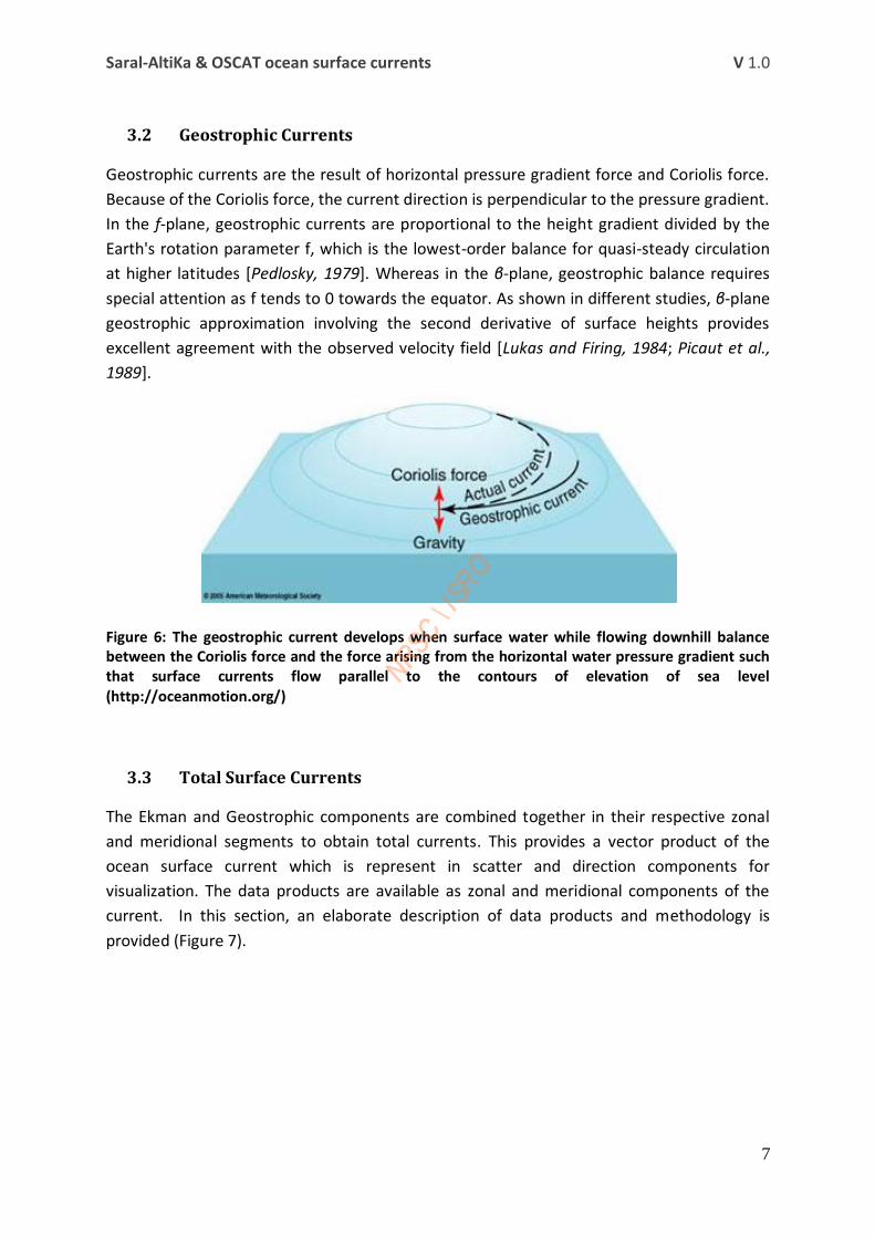
3.2 Geostrophic Currents

Geostrophic currents are the result of horizontal pressure gradient force and Coriolis force.

Because of the Coriolis force, the current direction is perpendicular to the pressure gradient.

In the f-plane, geostrophic currents are proportional to the height gradient divided by the

Earth's rotation parameter f, which is the lowest-order balance for quasi-steady circulation

at higher latitudes [Pedlosky, 1979]. Whereas in the β-plane, geostrophic balance requires

special attention as f tends to 0 towards the equator. As shown in different studies, β-plane

geostrophic approximation involving the second derivative of surface heights provides

excellent agreement with the observed velocity field [Lukas and Firing, 1984; Picaut et al.,

1989].

Figure 6: The geostrophic current develops when surface water while flowing downhill balance between the Coriolis force and the force arising from the horizontal water pressure gradient such that surface currents flow parallel to the contours of elevation of sea level (http://oceanmotion.org/)

3.3 Total Surface Currents

The Ekman and Geostrophic components are combined together in their respective zonal

and meridional segments to obtain total currents. This provides a vector product of the

ocean surface current which is represent in scatter and direction components for

visualization. The data products are available as zonal and meridional components of the

current. In this section, an elaborate description of data products and methodology is

provided (Figure 7).


8

Figure 7: Flow diagram of the Currents estimation using OSCAT & Saral-AltiKa data.

The output data files are available in NETCDF (.nc) format. The images for gridded SSH,

Ekman currents, Geostrophic currents and Total currents are provided in PNG image format.

Gridded SSH has been computed using previous 15-days along track Saral-AltiKa OGDR and

GDR products (Description is provided in next section). Figure 6 presents the flow diagram

of the procedure followed for generation of daily products.

3.4 Nomenclature

Input and output file naming conventions are mentioned below: Input file: OSCAT-L 2B : S1L2BYYYYDDD_NNNNN_MMMMM.h5

AltiKa GDR : SRL_GPN_2PTPCCC_PASS_YYYYMMDD_*1_ YYYYMMDD_*2.CNES.nc

Output data file:

GEOSTROPHIC CURRENTS MAPS

COMPUTATION OF WIND STRESS &

EKMAN CURRENTS

OSCAT WIND FIELDS LEVEL – 2B ALONG TRACK

MERIDIONAL AND ZONAL WIND COMPONENTS

DATA INTERPOLATING VARIATIONAL

ANALYSIS (DIVA)

COMPUTATION OF GEOSTOPHIC CURRENTS

Saral-AltiKa GDR NATIVE

DATA FILTERING & GRIDDING

SEA SURFACE HEIGHT (SSH) & MEAN DYNAMIC

TOPOGRAPHY (MDT)

SSH MAPS

TOTAL CURRENTS

MAPS & DATA IN NETCDF FORMAT

EKMAN CURRENTS MAPS


9

Total Currents : SRLP_TTT_YYYYMMDD.nc

Geostrophic Currents : SRLP_TTT_YYYYMMDD.nc

Output images: Ekman Currents: OC2S_TTT_YYYYMMDD1_ YYYYMMDD2.png

Geostrophic Currents: SRLP_TTT_ YYYYMMDD1_ YYYYMMDD2.png

Sea Surface Height: SRLP_TTT_ YYYYMMDD1_ YYYYMMDD2.png

Total Currents: SRLP_TTT_ YYYYMMDD1_ YYYYMMDD2.png

Where,

YYYY : The calendar year when data was acquired.

MM : The month when data was acquired.

DD : The day of the month when data was acquired.

DDD : The day of the year when data was acquired.

YYYYMMDD1: Start Day (first day)

YYYYMMDD2: End Day (last day)

*1 : Data acquisition start time (HHMMSS).

*2 : Data acquisition end time (HHMMSS).

P : G GDR

I IGDR

O OGDR

TTT : Product Type

TSC Total Surface Currents

GEO Geostrophic Currents

EKM Ekman Currents

SSH Sea Surface Height

For more information on OSCAT-2 products, visit http://www.nrsc.gov.in/ and for Saral-AltiKa products, visit http://www.aviso.oceanobs.com/.

3.5 Data Processing Steps

The methodology for obtaining surface currents from satellites involves effectively and

efficiently combining the Sea Surface Height (SSH) or Absolute Dynamic Topography (ADT)

data from altimeters with the wind velocity data from scatterometers. All the current

products are generated only for the Indian Ocean (30oS to 30oN and 30oE to 120oE). MATLAB

tools have been used for the computation and generation of output products. The following

steps have been adopted for the derivation of products:

Estimation of Ekman Currents:

http://www.nrsc.gov.in/

http://www.aviso.oceanobs.com/


10

For the wind-driven (Ekman) currents, the Ekman components (ue,ve) are given by [Van

Meurs & Niiler, 1999]:

....................(1)

Where [ue, ve] are the zonal and meridional ekman current components, respectively. is

the density of water (1025 kgm-3), h is the wind mixing depth and r is a linear drag

coefficient that represents vertical viscosity terms. τx and τy represent the Wind stress

components, which have been directly taken from the products available at NICES portal of

Bhuvan website. These stress components are computed as:

............................(2)

where, CD is a dimensionless coefficient called drag coefficient. Non-linear drag coefficient

(CD) based on Large & Pond (1981) modified for low wind speeds [Trenberth et al., 1990] is

used.

W is the wind speed (taken from Daily Wind Composites products available at NICES portal),

is the angle of wind vector from true north and is the density of air (1.2 kg/m3). Finally it comes out to be:

..................(3)

Lagerloef et al. (1999) performed a regression analysis and found values of r = 2.15 x 10-4

ms-1 and h = 32.5 m, which remain fairly constant over the tropical band. We have used the

same values in our analysis.

As the wind composite products are available at the spatial resolution of 0.5°0.5°, for

generation of Ekman currents, the products are regridded at spatial resolution of

0.25°0.25°. The ekman currents products are available at the quarter degree resolution for

the Indian Ocean.

Gridding of SSH and MDT:

SSH and MDT data has been gridded at a spatial resolution of 0.25°0.25° for the complete

global. For gridding, Saral-AltiKa GDR native data set for the last 15 days has been filtered

ue + ive = Beiφ

(τx + iτy);

B =

, φ = arctan

τx = airCDW2sin τy = airCDW

2cos

ue =

( rτx + fhτy)

ve =

( rτy fhτx)


11

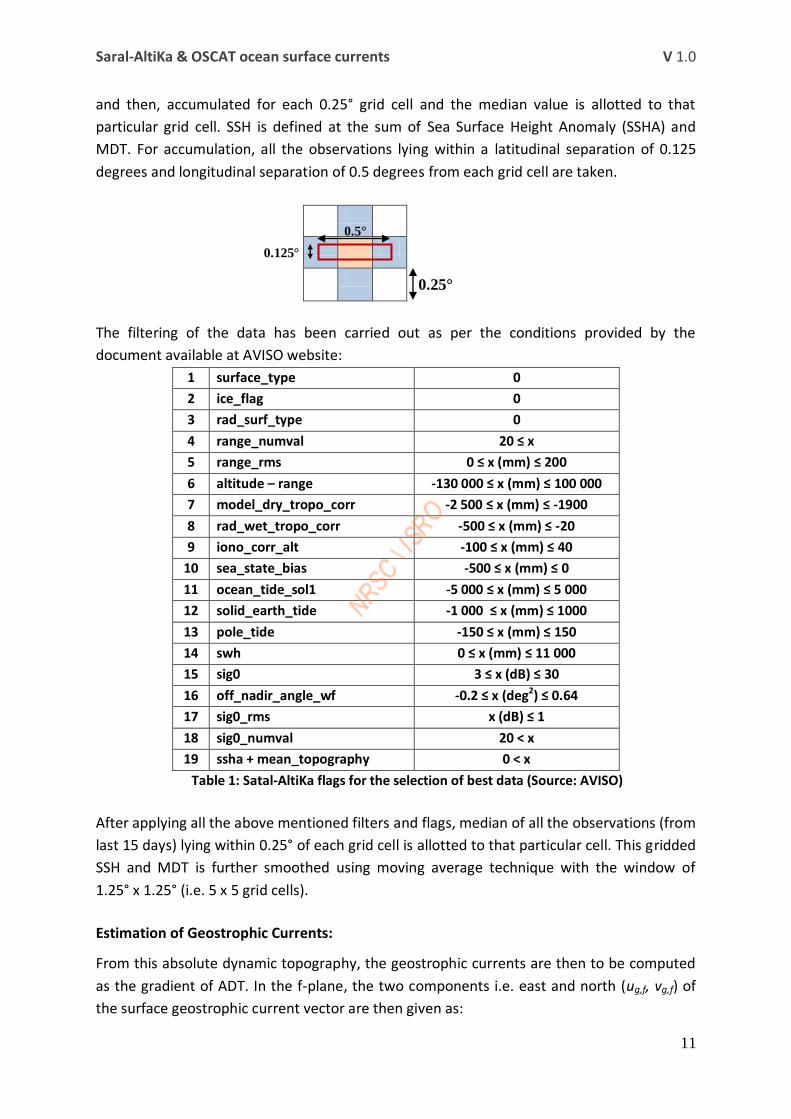
and then, accumulated for each 0.25° grid cell and the median value is allotted to that

particular grid cell. SSH is defined at the sum of Sea Surface Height Anomaly (SSHA) and

MDT. For accumulation, all the observations lying within a latitudinal separation of 0.125

degrees and longitudinal separation of 0.5 degrees from each grid cell are taken.

The filtering of the data has been carried out as per the conditions provided by the

document available at AVISO website:

1 surface_type 0

2 ice_flag 0

3 rad_surf_type 0

4 range_numval 20 ≤ x

5 range_rms 0 ≤ x (mm) ≤ 200

6 altitude – range -130 000 ≤ x (mm) ≤ 100 000

7 model_dry_tropo_corr -2 500 ≤ x (mm) ≤ -1900

8 rad_wet_tropo_corr -500 ≤ x (mm) ≤ -20

9 iono_corr_alt -100 ≤ x (mm) ≤ 40

10 sea_state_bias -500 ≤ x (mm) ≤ 0

11 ocean_tide_sol1 -5 000 ≤ x (mm) ≤ 5 000

12 solid_earth_tide -1 000 ≤ x (mm) ≤ 1000

13 pole_tide -150 ≤ x (mm) ≤ 150

14 swh 0 ≤ x (mm) ≤ 11 000

15 sig0 3 ≤ x (dB) ≤ 30

16 off_nadir_angle_wf -0.2 ≤ x (deg2) ≤ 0.64

17 sig0_rms x (dB) ≤ 1

18 sig0_numval 20 < x

19 ssha + mean_topography 0 < x

Table 1: Satal-AltiKa flags for the selection of best data (Source: AVISO)

After applying all the above mentioned filters and flags, median of all the observations (from

last 15 days) lying within 0.25° of each grid cell is allotted to that particular cell. This gridded

SSH and MDT is further smoothed using moving average technique with the window of

1.25° x 1.25° (i.e. 5 x 5 grid cells).

Estimation of Geostrophic Currents:

From this absolute dynamic topography, the geostrophic currents are then to be computed

as the gradient of ADT. In the f-plane, the two components i.e. east and north (ug,f, vg,f) of

the surface geostrophic current vector are then given as:

0.25°

0.125°

0.5°


12

.............................(4)

where, g is the acceleration due to gravity, f is the Coriolis parameter (f = 2 Ω sin φ), and ζ is the height of the sea surface above a level surface (ADT). φ is the latitude and Ω is the angular velocity of the earth's rotation (Ω = 7.29x10-5 sec-1). In the β-plane, as shown by Lagerloef at al. (1999) the geostrophic currents (ug,β, vg,β) are computed as:

.............................(5)

where, β =

.

For the equatorial region, β is a constant given by β = 2 Ω/r = 2.3 x 10-11 m-1s-1. Picaut et al. (1989) also state that the second derivative is valid over spatial scales of > 100 km and timescales greater than 15-30 days, providing relatively smoothed geostrophic velocities at the equator. The computation of Geostrophic currents in the Indian equatorial region requires further investigation.

The final currents are then a linear combination of geostrophic and wind-driven (Ekman) motion given as:

...............................(6)

where, Ūg and Ūe are the Geostrophic and Ekman components, respectively.

4. Results and Discussion

The Saral-AltiKa and OSCAT derived ocean surface currents have been compared with CNES

AVISO geostrophic currents and NOAA OSCAR total currents for the year 2013 (i.e. 28th Mar,

2013 to 31st Dec, 2013 ). Both the AVISO and OSCAR currents data are available at spatial

resolution of 0.33° with temporal resolution of daily and 5 days respectively. The datasets

are regridded to the spatial resolution of 0.25° using nearest neighborhood method. The

results have been indicated. The validation of the currents is still in progress, but the

preliminary results are very promising. The comparisons are also carried out at different

spatial and temporal resolutions.

4.1 Comparison with AVISO Geostrophic currents

The comparison results of Saral-AltiKa derived geostrophic currents with AVISO geostrophic currents are shown in Tables 2 & 3. As can be seen, geostrophic currents in f-plane show better correlation than those in β-plane. This can be attributed to Coriolis parameter which

ug,β =

, vg,β =

Ū = Ūg + Ūe

ug,f =

, vg,f =


13

approaches zero in the β-plane. Also, the zonal component of geostrophic currents shows better correlation than meridional component. The bias in currents speed (f-plane) varies in the range of 3.5 – 4.5 cm/s. The correlation is highest for the months of August and September. As the products are still in testing phase, it will be difficult to comment on the causes of these discrepancies.

Month R_U R_V R_W Bias_U Bias_V Bias_W

Mar 0.46 0.32 0.35 -0.01 0.83 3.50

Apr 0.51 0.31 0.42 -0.32 0.77 4.07

May 0.55 0.33 0.45 0.32 0.90 4.35

Jun 0.53 0.36 0.44 0.57 0.86 4.68

Jul 0.56 0.37 0.46 0.08 1.07 4.41

Aug 0.60 0.40 0.49 -0.33 0.79 3.45

Sep 0.60 0.40 0.49 -0.46 0.71 3.56

Oct 0.57 0.40 0.43 -0.15 0.69 3.82

Nov 0.54 0.40 0.37 0.59 0.67 4.37

Dec 0.54 0.37 0.42 0.25 0.39 4.26

Table 2: AVISO versus Saral-AltiKa derived geostrophic currents for 2013. Monthly mean values of

correlation coefficient (R) and bias (in cm/s) have been indicated for zonal(U), meridional (V) and total (W)

currents.


Mar 0.66 0.46 0.50 0.79 0.28 -1.25

Apr 0.65 0.45 0.50 0.66 0.20 0.02

May 0.66 0.44 0.51 0.40 0.15 0.04

Jun 0.66 0.48 0.55 0.50 0.34 0.15

Jul 0.72 0.53 0.61 0.17 0.42 -0.60

Aug 0.74 0.53 0.63 0.30 0.21 -0.92

Sep 0.74 0.53 0.64 0.10 0.29 -0.87

Oct 0.72 0.53 0.58 0.18 0.31 -0.82

Nov 0.71 0.55 0.54 0.38 0.21 -1.05

Dec 0.69 0.51 0.55 0.38 0.24 -0.85

Table 3: AVISO versus Saral-AltiKa derived geostrophic currents in the f-plane (|latitude| > 5) for 2013.

Monthly mean values of correlation coefficient (R) and bias (in cm/s) have been indicated for zonal (U),

meridional (V) and total (W) currents.

4.2 Comparison with OSCAR total currents

The comparison results of Saral-AltiKa and OSCAT derived total currents with OSCAR geostrophic currents are shown in Table 4 & 5. As was observed in the case of AVISO, currents in f-plane show better correlation than those in β-plane. Also, the zonal component of currents shows better correlation than meridional component. The bias in currents speed (f-plane) has now reduced to the range of 1 – 3 cm/s. In this case also, the correlation is highest for the months of August and September.


14


Mar 0.49 0.41 0.55 2.31 0.10 0.13

Apr 0.52 0.32 0.55 -0.23 0.40 1.58

May 0.62 0.34 0.60 -0.29 0.39 1.12

Jun 0.57 0.35 0.57 1.93 -0.63 3.84

Jul 0.54 0.37 0.56 1.20 0.60 3.03

Aug 0.60 0.40 0.60 0.46 0.43 2.64

Sep 0.67 0.47 0.61 -0.57 0.05 2.55

Oct 0.62 0.47 0.58 0.92 0.20 2.59

Nov 0.59 0.46 0.56 0.61 0.37 2.90

Dec 0.67 0.42 0.62 -0.66 -0.67 2.69

Table 4: OSCAR versus Saral-AltiKa derived total currents for 2013. Monthly mean values of correlation

coefficient (R) and bias (in cm/s) have been indicated for zonal(U), meridional (V) and total (W) currents.


Mar 0.72 0.54 0.54 0.26 -0.71 -0.51

Apr 0.70 0.49 0.54 1.04 0.26 0.91

May 0.72 0.47 0.55 0.57 -0.65 1.05

Jun 0.77 0.51 0.58 1.01 -2.13 2.87

Jul 0.78 0.53 0.64 0.59 -1.36 1.64

Aug 0.81 0.57 0.68 0.46 -1.32 1.64

Sep 0.83 0.61 0.70 0.11 -0.88 1.46

Oct 0.80 0.60 0.64 0.35 -0.27 1.02

Nov 0.78 0.62 0.59 0.24 0.43 0.84

Dec 0.77 0.58 0.60 -0.09 0.42 1.35

Table 5: OSCAR versus Saral-AltiKa derived total currents in the f-plane (|latitude| > 5) for 2013. Monthly

mean values of correlation coefficient (R) and bias (in cm/s) have been indicated for zonal (U), meridional

(V) and total (W) currents.

4.3 Comparison with moored buoy total currents

The currents from satellite and INCOIS moored buoys have been compared and the results

are indicated in figure 8 & 9. The comparisons have been carried out at different spatial and

temporal resolutions. A preliminary analysis indicated that the satellites derived currents

exhibit better correlation in Bay of Bengal region rather than Arabian Sea region. This may

be attributed to general feature of low surface currents in Arabian Sea. It has also been

observed that comparison at 50 km spatial resolution shows better results.


15

Figure 8: (Left) Comparison of OSCAT and Saral-AltiKa derived ocean surface zonal currents with INCOIS moored buoy ocean zonal currents at 25 km spatial resolution on monthly basis for Bay of Bengal region. (Right) Comparison of OSCAT and Saral-AltiKa derived ocean surface zonal currents with INCOIS moored buoy ocean zonal currents at 100 km spatial resolution on weekly basis for Bay of Bengal region.

Figure 9: (Left) Comparison of OSCAT and Saral-AltiKa derived ocean surface meridional currents with INCOIS moored buoy ocean meridional currents at 25 km spatial resolution on monthly basis for Bay of Bengal region. (Right) Comparison of OSCAT and Saral-AltiKa derived ocean surface meridional currents with INCOIS moored buoy ocean meridional currents at 50 km spatial resolution on 15 days mean basis for Bay of Bengal region.

Please note that INCOIS moored buoys measure ocean currents at 3 metres depth.

Further improvement in algorithm can be expected in upcoming versions of the same

document.

As Saral-AltiKa derived geostrophic currents can be estimated using OGDR data, the

products are generated on real time basis. The processing is done in real time, with

geostrophic currents already estimated from 28th March, 2013 onwards on daily basis. But

as OSCAT data is only available till February, 2014, the total surface currents are available

for the period of March, 2013 to February, 2014. For an example, map of Saral-AltiKa

derived geostrophic currents is shown in figure 10. As can be observed from the figure,

major gyre systems and general circulation pattern in the Indian Ocean region can be easily

distinguished. The Somalia region gyre is further discussed in next figure.


16

As shown in figure 10, the net geostrophic currents flow in the western equatorial region is

eastward, whereas in the northern part of eastern equatorial region, it is eastward. Also, the

major gyre systems are prominently evident in the currents maps.

Figure 10: Saral-AltiKa derived Geostrophic currents for 04 June, 2014. The red arrows indicate the gyre

systems and the general flow pattern.

Similar Indian Ocean total surface maps have been generated on daily basis. In the next

figure, high resolution images of total ocean surface currents are shown for Somali and Bay

of Bengal region.

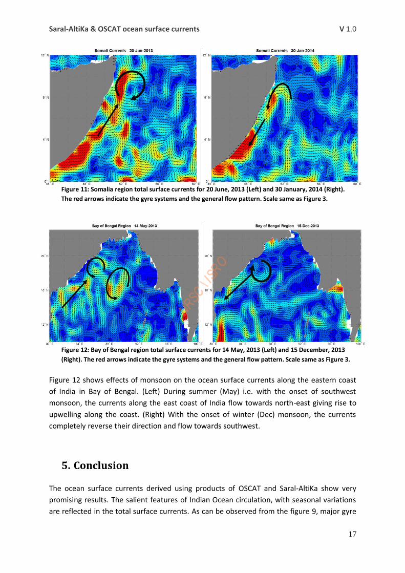
Figure 11 shows Somali current system, which varies significantly with time. (Left) During

summer (June) i.e. southwest monsoon, the Somali currents flow towards north-east giving

rise to upwelling along the coast of Somalia. (Right) With the onset of winter (Jan) monsoon,

the Somali currents completely reverse their direction and flow towards southwest along

the Somalia coast, and thereby, no upwelling.


17

Figure 11: Somalia region total surface currents for 20 June, 2013 (Left) and 30 January, 2014 (Right).

The red arrows indicate the gyre systems and the general flow pattern. Scale same as Figure 3.

Figure 12: Bay of Bengal region total surface currents for 14 May, 2013 (Left) and 15 December, 2013

(Right). The red arrows indicate the gyre systems and the general flow pattern. Scale same as Figure 3.

Figure 12 shows effects of monsoon on the ocean surface currents along the eastern coast

of India in Bay of Bengal. (Left) During summer (May) i.e. with the onset of southwest

monsoon, the currents along the east coast of India flow towards north-east giving rise to

upwelling along the coast. (Right) With the onset of winter (Dec) monsoon, the currents

completely reverse their direction and flow towards southwest.

5. Conclusion

The ocean surface currents derived using products of OSCAT and Saral-AltiKa show very

promising results. The salient features of Indian Ocean circulation, with seasonal variations

are reflected in the total surface currents. As can be observed from the figure 9, major gyre


18

systems and general circulation pattern in the Indian Ocean region can be easily

distinguished. The Somalia region gyre is further discussed in next figure. Also, the

preliminary validation results at different spatial and temporal resolutions with INCOIS

buoys show promising correlation coefficient (R2) ranging from 0.52 to 0.64. Bias for zonal

currents is more negative (≈ −4 cm/s) than that for meridional component (≈ −2 cm/s).

There is a scope for better results by performing global validation and fine tuning of

algorithm. Better results can be expected in the upcoming versions of total surface currents.

Acknowledgements: We take it as a deemed privelege to express our sincere thanks to all concerned who have contributed either directly or indirectly for the successful completion of ocean surface currents computation and product generation using Saral-AltiKa altimeter and Oceansat-2 scatterometer data. The work is a part of Techincal Development Project (TDP) at NRSC and SARAL-AltiKa User Promotion activity of ISRO. We are highly grateful to Dr. V. K. Dadhwal, Director NRSC for his encouragement and guidance during this study. NDC team and network support group of NRSC and last but not the least OSCAT project team are sincerely acknowledged for successfully making OSCAT data available to the users.


19

6. References

AVISO User Handbook Ssalto/Duacs: M(SLA) and M(ADT) Near-Real Time and Delayed-

Time, SALP-MU-P-EA-21065-CLS, edition 4.1, May 2014 (AVISO - Archiving, Validation

and Interpretation of Satellite Oceanographic Data) www.oceanobs.aviso.com

Bonjean, F. and Gary S. E. Lagerloef (2002), Diagnostic model and analysis of the surface

currents in the tropical Pacific ocean, J. Phys. Oceanogr., 32, 29382954.

Dorandeu, J. and P. Y. Le Traon (1999), Effects of global mean atmospheric pressure

variations on mean sea level changes from TOPEX/Poseidon, J. Atmos. Oceanic Technol.,

16, 1279–1283.

Ducet, N., P. Y. Le Traon and G. Reverdin (2000), Global high resolution mapping of ocean

circulation from TOPEX/Poseidon and ERS 1 and 2, J. Geophys. Res., 105 (C8), 19,477-

19,498.

Lagerloef, G. S. E., G. T. Mitchum, R. Lukas and P. P. Niiler (1999), Tropical pacific near

surface currents estimated from altimeter, wind and drifter data, J. Geophys. Res., 104,

23,313–23,326.

Le Traon, P.-Y. and F. Ogor( 1998), ERS-1/2 orbit improvement using TOPEX/Poseidon:

The 2 cm challenge, J. Geophys. Res., 103, 8045–8057.

Lukas, R. and E. Firing, 1984: The geostrophic balance of the Pacific Equatorial

Undercurrent, Deep-Sea Res., 31, 61–66.

OSCAT Product Handbook, Version 1.3, Dec. 2011.

Price, J. F., R. A. Weller and R. R. Schudlich (1987), Wind-Driven Ocean Currents and

Ekman Transport, Science, 238 (4833), 1534-1538.

Geophysical fluid dynamics, Joseph Pedlosky. Springer-Verlag, Berlin,1979

Philander, S. G. H. and R. C. Pacanowski (1980), The generation of equatorial currents, J.

Geophys. Res., 85, 1,123–1,136.

Picaut J, Hayes SP, McPhaden MJ (1989) Use of the geostrophic approximation to estimate

time-varying zonal currents at the equator. J Geophys Res 94:3228–3236.

Ralph, E. A. and P. P. Niiler (1999), Wind-driven currents in the tropical pacific, J. Phys.

Oceanogr., 29, 2121–2129.

Saral-AltiKa Products Handbook, SALP-MU-M-OP-15984-CN, Issue 2.3, July 2013.

Seidel HF, Giese BS (1999) Equatorial currents in the Pacific Ocean 1992–1997. J Geophys

Res 104:7849–7863

Stommel, H. (1960), Wind-drift near the equator, Deep Sea Res., 6, 298–302.

http://www.aviso.altimetry.fr/fileadmin/documents/data/tools/hdbk_duacs.pdf

http://www.aviso.altimetry.fr/fileadmin/documents/data/tools/hdbk_duacs.pdf

www.oceanobs.aviso.com


20

Sudre,J. and R. Morrow (2008), Global surface currents: a high-resolution product for

investigating ocean dynamics, Ocean Dynamics, DOI 10.1007/s10236-008-0134-9.

K.E. Trenberth, W.G. Large & J.G. Olson, 1990, “The Mean Annual Cycle in Global Ocean

Wind Stress”, J.Physical Oceanography, Vol. 20, pp. 1742 – 1760.

Van Meurs P, Niiler PP (1997), Temporal variability of the large-scale geostrophic surface

velocity in the northeast Pacific, J. Phys. Oceanogr., 27:2288–2297

W. G. Large & S. Pond., 1981,“Open Ocean Measurements in Moderate to Strong Winds”,

J. Physical Oceanography, Vol. 11, pp. 324 - 336.

7. Appendix

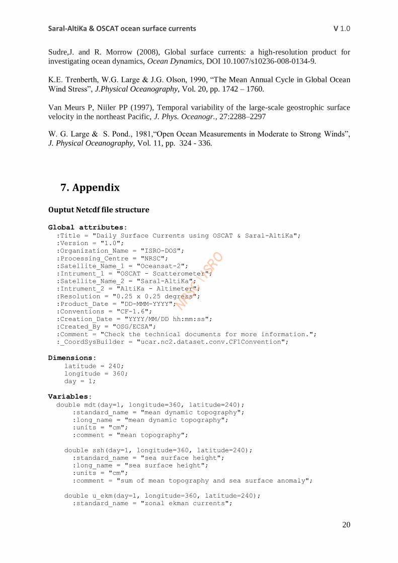
Ouptut Netcdf file structure

Global attributes:

:Title = "Daily Surface Currents using OSCAT & Saral-AltiKa";

:Version = "1.0";

:Organization_Name = "ISRO-DOS";

:Processing_Centre = "NRSC";

:Satellite_Name_1 = "Oceansat-2";

:Intrument_1 = "OSCAT - Scatterometer";

:Satellite_Name_2 = "Saral-AltiKa";

:Intrument_2 = "AltiKa - Altimeter";

:Resolution = "0.25 x 0.25 degress";

:Product_Date = "DD-MMM-YYYY";

:Conventions = "CF-1.6";

:Creation_Date = "YYYY/MM/DD hh:mm:ss";

:Created_By = "OSG/ECSA";

:Comment = "Check the technical documents for more information.";

:_CoordSysBuilder = "ucar.nc2.dataset.conv.CF1Convention";

Dimensions:

latitude = 240;

longitude = 360;

day = 1;

Variables:

double mdt(day=1, longitude=360, latitude=240);

:standard_name = "mean dynamic topography";

:long_name = "mean dynamic topography";

:units = "cm";

:comment = "mean topography";

double ssh(day=1, longitude=360, latitude=240);

:standard_name = "sea surface height";

:long_name = "sea surface height";

:units = "cm";

:comment = "sum of mean topography and sea surface anomaly";

double u_ekm(day=1, longitude=360, latitude=240);

:standard_name = "zonal ekman currents";


21

:long_name = "zonal ekman currents";

:units = "cm/s";

:comment = "Wast-east component of Ekman Currents";

double v_ekm(day=1, longitude=360, latitude=240);

:standard_name = "meridional ekman currents";

:long_name = "meridional ekman currents";

:units = "cm/s";

:comment = "South-north component of Ekman Currents";

double u_geo(day=1, longitude=360, latitude=240);

:standard_name = "zonal geostrophic currents";

:long_name = "zonal geostrophic currents";

:units = "cm/s";

:comment = "Wast-east component of Geostrophic Currents";

double v_geo(day=1, longitude=360, latitude=240);

:standard_name = "meridional geostrophic currents";

:long_name = "meridional geostrophic currents";

:units = "cm/s";

:comment = "South-north component of Geostrophic Currents";

double u_total(day=1, longitude=360, latitude=240);

:standard_name = "zonal surface currents";

:long_name = "zonal total ocean surface currents";

:units = "cm/s";

:comment = "Computed by adding zonal components of Ekman &

Geostrophic Currents.";

double v_total(day=1, longitude=360, latitude=240);

:standard_name = "meridional surface currents";

:long_name = "meridional total ocean surface currents";

:units = "cm/s";

:comment = "Computed by adding meridional components of Ekman &

Geostrophic Currents.";

double latitude(latitude=240);

:standard_name = "latitude";

:long_name = "latitude";

:units = "degrees_north";

:limits = "-30N to 30N in degrees";

:comment = "Positive latitude is North latitude, negative latitude is

South latitude.";

:_CoordinateAxisType = "Lat";

double longitude(longitude=360);

:standard_name = "longitude";

:long_name = "longitude";

:units = "degrees_east";

:limits = "30E to 120E in degrees";

:comment = "East longitude relative to Greenwich meridian.";

:_CoordinateAxisType = "Lon";

int day(day=1);

:standard_name = "day";

:long_name = "day number";

:units = "days since 2000-1-0";

:comment = "Day number since 1-Jan-2000. 1-Jan-2000 is Day number

1.";

:_FillValue = -99999; // int

Ocean Sciences Group (Earth and Climate Science Area) National Remote Sensing Centre ISRO (Govt. of India, Dept. of Space) Balanagar, Hyderabad – 500037, INDIA

NR

SC

– E

CSA

– O

SG

– N

OV

- 20

14

– T

R –

65

9

Documents

Indian Ocean Surface Currents Using OSCAT and Saral-AltiKa · Being a land-locked area, unlike the Pacific and the Atlantic Ocean, the topography introduces diversities into the ocean