Embed Size (px)
Citation preview

OSTST - March 2007 - Hobart 1
Impacts of atmospheric attenuations on Impacts of atmospheric attenuations on AltiKa expected performancesAltiKa expected performances
J.D. Desjonquères J.D. Desjonquères (1)(1), N. Steunou, N. Steunou(1)(1)
A. QuesneyA. Quesney(2)(2)
P. SengenesP. Sengenes(1)(1), J. Lambin, J. Lambin(1)(1)
J. TournadreJ. Tournadre(3)(3)
(1)(1) CNES, France CNES, France(2) (2) NOVELTIS, FranceNOVELTIS, France(3) (3) IFREMER, FranceIFREMER, France

OSTST - March 2007 - Hobart 2
IntroductionMethod of simulationSimulated clouds : effect on Ka and Ku measurementUse of MODIS dataSimulation of return waveforms above MODIS tracks
Impacts on range, SWH in several real clouds configurations Comparison Ka/Ku
Statistical study Classification of atmospheric attenuation scenes Results
Conclusion / Perspectives
ContentsContents
OSTST - March 2007 - Hobart 3
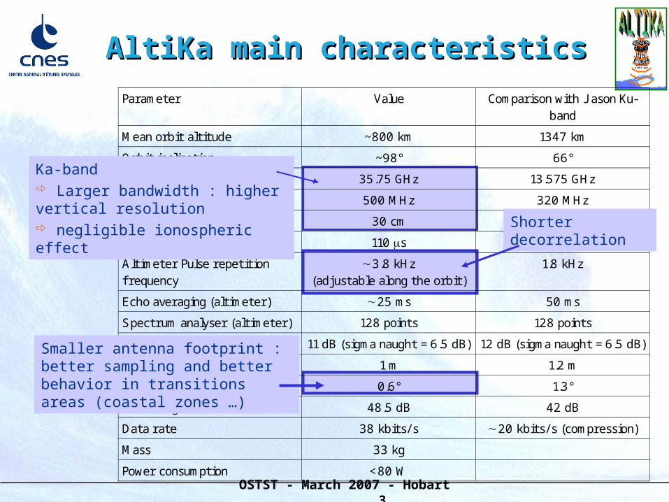
AltiKa main characteristicsAltiKa main characteristics
Parameter Value Comparison with J ason Ku-band
Mean orbit altitude ~800 km 1347 km
Orbit inclination ~98° 66°
Altimeter band 35.75 GHz 13.575 GHz
Pulse bandwidth 500 MHz 320 MHz
Vertical resolution 30 cm 47 cm
Pulse duration 110 s 110 s
Altimeter Pulse repetition f requency
3.8 kHz (adjustable along the orbit)
1.8 kHz
Echo averaging (altimeter) 25 ms 50 ms
Spectrum analyser (altimeter) 128 points 128 points
Altimeter Link budget 11 dB (sigma naught = 6.5 dB) 12 dB (sigma naught = 6.5 dB)
Antenna diameter 1 m 1.2 m
Antenna aperture 0.6° 1.3°
Antenna gain 48.5 dB 42 dB
Data rate 38 kbits/ s 20 kbits/ s (compression)
Mass 33 kg
Power consumption < 80 W
Ka-band Larger bandwidth : higher vertical resolution negligible ionospheric effect
Smaller antenna footprint : better sampling and better behavior in transitions areas (coastal zones …)
Shorter decorrelation

OSTST - March 2007 - Hobart 4
AltiKa expected performancesAltiKa expected performances Expected range measurement noise (1 Hz) on ocean surfaces
Accuracy of the altimeter range measurement over sea surface : about 1 cm for a SWH of 2 meters Improvement of about 40% on the range noise versus Ku-band performances
1 second range noise (cm) versus SWH in Ku- and Ka-bands1 second range noise (cm) versus SWH in Ku- and Ka-bands
OSTST - March 2007 - Hobart 5
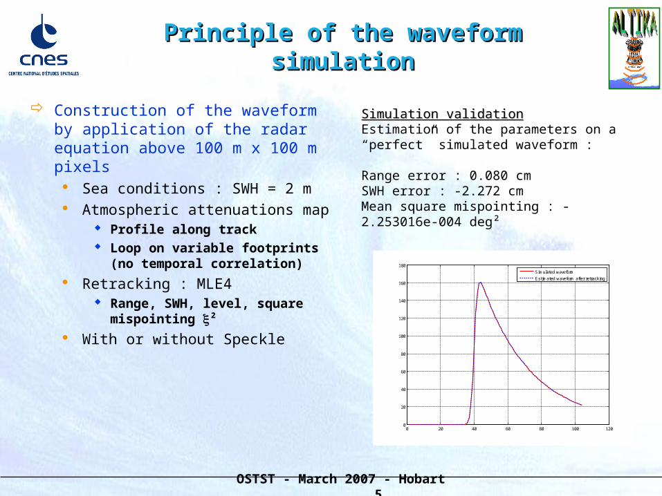
Principle of the waveform simulationPrinciple of the waveform simulation
Construction of the waveform by application of the radar equation above 100 m x 100 m pixels
Sea conditions : SWH = 2 m Atmospheric attenuations map
Profile along track Loop on variable footprints (no
temporal correlation) Retracking : MLE4
Range, SWH, level, square mispointing ²
With or without Speckle
Simulation validationSimulation validationEstimation of the parameters on a “perfect” simulated waveform :
Range error : 0.080 cmSWH error : -2.272 cmMean square mispointing : -2.253016e-004 deg²
0 20 40 60 80 100 1200
20
40
60
80
100
120
140
160
180
Simulated waveform
Estimated waveform after retracking

OSTST - March 2007 - Hobart 6
Atmospheric attenuations mapAtmospheric attenuations map
Simulated clouds characterized by Cloud size (length, width, height Hc) and positioning on the track Att_dB = 2 Hc kp with kp = LWC.
Ka = 1.070049578 (dB/km)/(g/m3) Ku = 0.16968466 (dB/km)/(g/m3)
Use of MODIS data (Noveltis and CNES study) Use of MODIS cloud product (MOD06), around 1 km-pixel
cloud water path (CWP), cloud phase (liquid or ice), cloud optical thickness, cloud particle effective radius are selected for our study
Att_dB = 2 kp x CWP with kp = LWC. Ka = 1.070049578 (dB/km)/(g/m3) for liquid or ice phase (worst case)
Interpolation of CWP data at 100 m - resolution
OSTST - March 2007 - Hobart 7
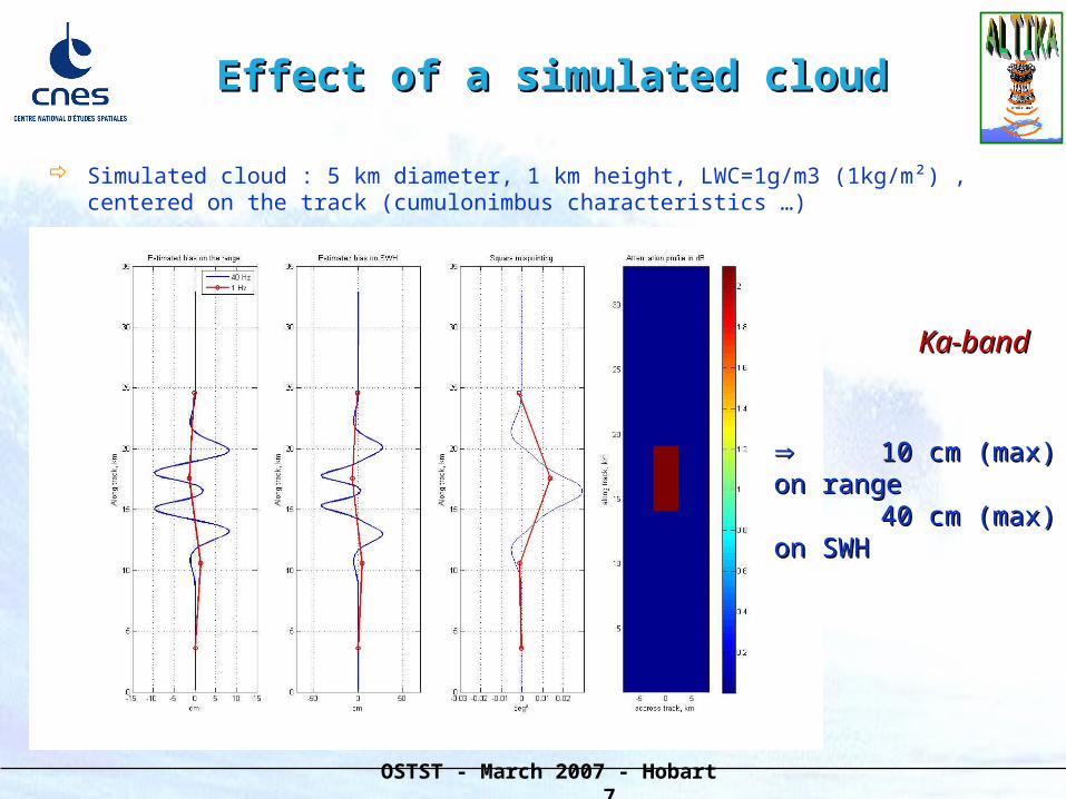
Effect of a simulated cloudEffect of a simulated cloud
Simulated cloud : 5 km diameter, 1 km height, LWC=1g/m3 (1kg/m²) , centered on the track (cumulonimbus characteristics …)
Ka-bandKa-band
10 cm (max) on 10 cm (max) on rangerange
40 cm (max) on 40 cm (max) on SWHSWH

OSTST - March 2007 - Hobart 8
Effect of a simulated cloudEffect of a simulated cloud Simulated cloud : 5 km diameter, 1 km height, LWC=1g/m3 (1kg/m²), centered on the
track (cumulonimbus characteristics …)
Ku-bandKu-band
4 cm (max) on range 20 cm (max) on SWH

OSTST - March 2007 - Hobart 9
Example of MODIS profile : typical weatherExample of MODIS profile : typical weather
Ka-band result :

OSTST - March 2007 - Hobart 10
Example of MODIS profile : typical weatherExample of MODIS profile : typical weather
Comparison of Ka/Ku-band errors for 40-Hz or 20-Hz data on the same profile
OSTST - March 2007 - Hobart 11
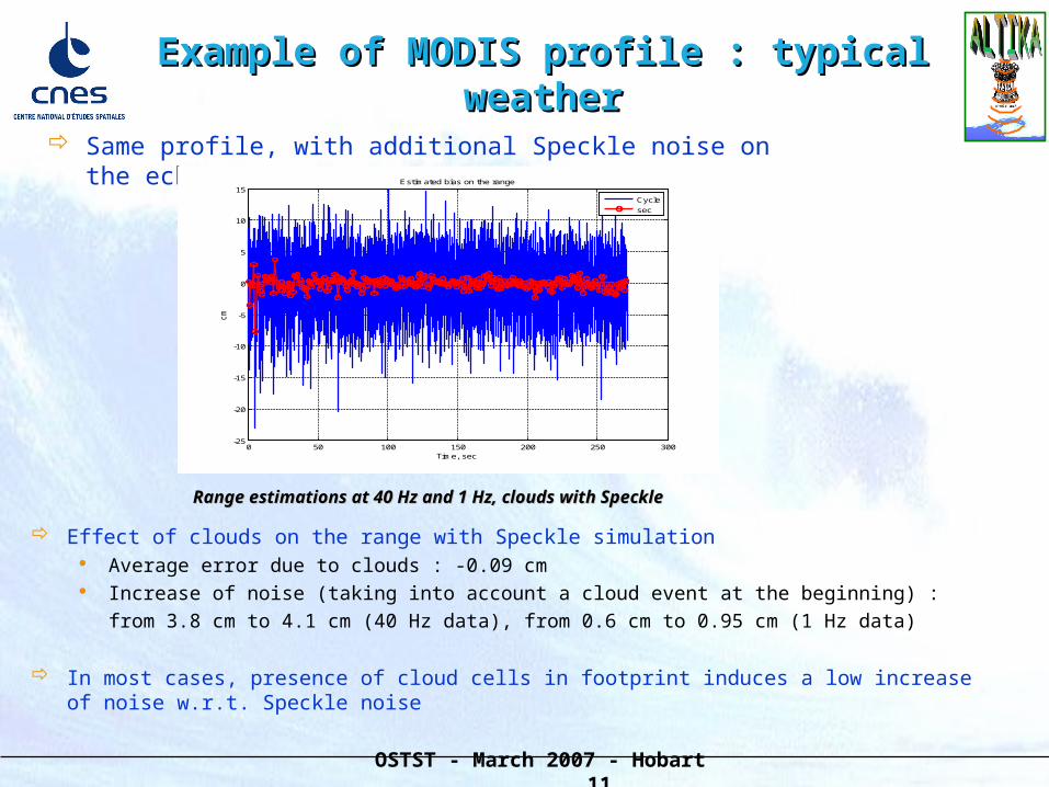
Example of MODIS profile : typical weatherExample of MODIS profile : typical weather
Same profile, with additional Speckle noise on the echoes :
0 50 100 150 200 250 300-25
-20
-15
-10
-5
0
5
10
15
Time, sec
cm
Estimated bias on the range
Cycle
sec
Effect of clouds on the range with Speckle simulation Average error due to clouds : -0.09 cm Increase of noise (taking into account a cloud event at the beginning) :
from 3.8 cm to 4.1 cm (40 Hz data), from 0.6 cm to 0.95 cm (1 Hz data)
In most cases, presence of cloud cells in footprint induces a low increase of noise w.r.t. Speckle noise
Range estimations at 40 Hz and 1 Hz, clouds with SpeckleRange estimations at 40 Hz and 1 Hz, clouds with Speckle

OSTST - March 2007 - Hobart 12
Other example of MODIS profile : high water content eventOther example of MODIS profile : high water content event
Evolutions of parameters estimations could be used to discriminate contaminated waveforms Rain effect, CNES/CLS study on rain rates from TRMM/TMI data shows that :
Average for one year and all geographical areas show that around 3% of data will be unavailable Unavailability can reach 10% locally depending on season (e.g. Bengal Golf)

OSTST - March 2007 - Hobart 13
Method
Extraction of 13km*13km scenes of attenuation from the MODIS “water content” product.
Classification
For each class, simulation of echoes affected by the characteristic attenuation.
Statistical processing
Statistical studyStatistical study
OSTST - March 2007 - Hobart 14
ClassificationClassification
Neuronal Classification of the attenuation profiles (differential attenuation in the footprint)
Input 11 724 250 scenes for the classification (12 days :1 day / month) 3 882 373 scenes for neuronal network training (4 days: 1 day / trimester)
Output A referent profile of attenuation for each class Cardinality of the classes Mean attenuation histogram for each class

OSTST - March 2007 - Hobart 15
Statistical resultsStatistical results
Ka band and SWH=2m
Atmospheric attenuation effect:
Range error < 0.1 cm : 85 % , < 1 cm : 93 %, < 2 cm : 96 %
SWH error < 1 cm : 88 % , < 5 cm : 95 %
OSTST - March 2007 - Hobart 16
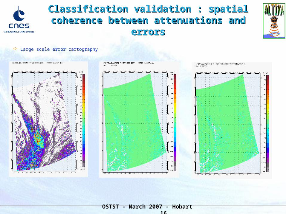
Classification validation : spatial coherence Classification validation : spatial coherence between attenuations and errorsbetween attenuations and errors
Large scale error cartography

OSTST - March 2007 - Hobart 17
Classification validation : spatial coherence Classification validation : spatial coherence between attenuations and errorsbetween attenuations and errors
local error cartography

OSTST - March 2007 - Hobart 18
ConclusionConclusion
Data unavailability due to clouds has been estimated : More than 90% of waveforms should be nominally processed We expect that most of contaminated waveforms could be processed
through dedicated algorithms results in representative situations (along track simulation with Speckle)
Averaging elementary data (e.g. from 40 Hz to 1 Hz) induces a reduction of the errors due to clouds
In typical situations, the effect of clouds is equivalent to an increase of noise measurement
Perspectives : A general study of waveforms classification is in progress To build editing method (see Jean TOURNADRE presentation) Study on geographical and seasonal availability is being performed (with
Noveltis)
![Conclusion - Université du Luxembourgorbilu.uni.lu/bitstream/10993/40087/1/Roelens Palerme... · Web viewAlexandre Dumas, Le Speronare [1843], Paris, Desjonquères, 1988, pp. 323](https://img.dokumen.tips/doc/110x75/5e4120f0bbc997527d6a0cc3/conclusion-universit-du-palerme-web-view-alexandre-dumas-le-speronare.jpg)