Embed Size (px)
Citation preview

776
ASCAT ocean
surface wind assessment
Giovanna De Chiara, Stephen English,
Peter Janssen, Jean-Raymond Bidlot
Research Department
July 2016

Series: ECMWF Technical Memoranda
A full list of ECMWF Publications can be found on our web site under:
http://www.ecmwf.int/en/research/publications
Contact: [email protected]
© Copyright 2016
European Centre for Medium Range Weather Forecasts
Shinfield Park, Reading, Berkshire RG2 9AX, England
Literary and scientific copyrights belong to ECMWF and are reserved in all countries. This publication is not to
be reprinted or translated in whole or in part without the written permission of the Director. Appropriate non-
commercial use will normally be granted under the condition that reference is made to ECMWF.
The information within this publication is given in good faith and considered to be true, but ECMWF accepts
no liability for error, omission and for loss or damage arising from its use.

ASCAT ocean surface wind assessment
Technical Memorandum No.776 1
Abstract
The European Centre for Medium-Range Weather Forecasts has been contracted by the European
Organization for the Exploitation of Meteorological Satellites (EUMETSAT) to perform an
evaluation of ASCAT wind measurements, assess their impact on the Global Observing System
(GOS) and optimize the assimilation strategy. This report presents the results of the work done during
the two years (February 2013-February 2015) of the contract (Project Ref.
EUM/CO/12/4600001149/JF).
The impact of the ASCAT-A and ASCAT-B winds has been assessed over different GOS scenarios:
one is replicating the operational ECMWF system and is using all the available observations; two
scenarios use a subset of the GOS (all observations except wind observations and all observations
except wind observations and AMSU-A) to assess the interaction between scatterometer
observations and other sensors.
The assessment of scatterometer winds has been performed using a range of diagnostics, from the
traditional forecast scores to the verification against independent observations such as altimeter
winds, wave height and wind speed buoy data. The verification methods show similar results.
The main positive impacts are made when either or both ASCAT datasets are assimilated together
with OSCAT data; ASCAT-A and ASCAT-B have the same impact on the system. From all the
verification methods, it is shown that, in a Full System configuration, the assimilation of
scatterometer observations is globally beneficial on the analysis; however the benefit is not
propagated into the forecast. Verifications against buoy and altimeter winds show that when other
wind observations are removed from the GOS, the positive impact of assimilating scatterometer
observations at analysis time is larger and is propagated to longer forecast range. Regional statistics
show that overall the largest benefit is coming from the Tropics.
The assimilation of ASCAT-B winds has a positive impact on the analysis departure of ASCAT-A.
It has a neutral to positive impact on the analysis departure of OSCAT in the Northern Hemisphere
and in the Tropics but is slightly negative in the Southern Hemisphere. This is most likely due to the
OSCAT wind speed bias seen in the Southern Ocean (mostly south of 50° S), which is known and
already partially corrected by KNMI. It is found that Scatterometer observations have impact only
up to 600 hPa; scatterometer assimilation appears to make almost no difference above this height.
This is also found to be the case for other near surface observations, especially wind, and it is not
specific to scatterometer observations. To better understand the ability of 4D-var to propagate the
scatterometer increments from the surface to higher model levels, single observation experiments
were run assimilating only one scatterometer observation close to the centre of a Tropical Cyclone
(TC) and in an area where the scatterometer wind and the model value were close. Results showed
that close to the TC, the 4D-Var is able to propagate the scatterometer wind information from the
surface to the upper troposphere. To assess the synergies of scatterometer observations with other
types of observation, experiments assimilating one scatterometer and a couple of AMSU-A
observations were run showing that the analysis increments structure is not modified when AMSU-
A observations are also assimilated, either at low or high model levels. This suggests that the large
impact of AMSU-A is not limiting the impact of ASCAT.
Forecast Error Contribution statistics show overall a higher impact for OSCAT winds due to the
higher number of assimilated observations. However, statistics computed for each single observation
show that a single ASCAT observation has higher impact than a single OSCAT observation.
ASCAT-A and ASCAT-B have the same impact. Moreover, regional statistics show that the largest
scatterometer observations impact is from the Southern Hemisphere.

ASCAT Ocean surface wind assessment
2 Technical Memorandum No.776
The impact of ASCAT winds has been evaluated on tropical cyclone events. Global statistics of mean
sea level pressure and storm centre position error do not show a clear benefit when assimilating
scatterometer winds when based on all the TCs occurring during the test period. However when the
analysis is repeated taking into account only TCs where scatterometer observations where available
at analysis time root mean square (RMS) forecast error of the minimum sea level pressure (SLP) in
the centre of the storm is reduced. It was found that during the test period the position errors for all
the configurations were, in general, small in comparison to model resolution, such that differences
in performance between the configurations were negligible.
A detailed analysis of the impact of ASCAT-A winds on the analysis and forecast of the Typhoon
Haiyan, which hit the Philippines in November 2013 has been performed. Overall the assimilation
of Scatterometer observations is beneficial for the storm analysis and forecast. However it was
noticed that some strong ASCAT winds in the area of maximum storm intensity were rejected prior
to the assimilation partially because of the thinning applied (only one observation out of four is
assimilated) and partially due to the quality control. If the wind vector difference between the
background and the observation is too high the observations are rejected. In this case, the wind vector
difference is likely due to a displacement of the storm location in the background. Tests were
performed for four TCs where this problem occurred, which showed that there is a general sensitivity
of the data assimilation to changes in thinning and quality control set-up. Preliminary tests on the use
of an alternative method to the current quality control, the Huber norm, were also run. This is a robust
method which allows observations with large background departure to still give some weight into
the analysis. The results showed that there is indeed potential to increase scatterometer impact further
through fine tuning of these components. This will be important for the new SCA scatterometers on
EPS-SG scatterometer, as it will better observe high winds.
The impact on the surface stress were also evaluated. The assimilation of scatterometer winds
increases the surface stress almost globally. Few areas in the Tropics showed lower values when the
observations are assimilated. Since surface stress is strongly connected to the surface winds, and in-
situ measurements are not available, the verification in few tropical sub-areas was done using
Altimeter and buoy winds. Results confirmed that the assimilation of scatterometer winds is
beneficial in these areas in terms of winds, and thus also in terms of surface stress.
1 Introduction
Scatterometer data are known to improve the quality of surface winds over the ocean. Therefore they
have an impact on the forecast skills of the atmospheric and wave models. In particular C-band
scatterometers, thanks to the microwave wavelength used, are capable to provide information also in the
presence of rainfall. Their observations are therefore important for the analysis of winds in case of
extreme events (usually characterized by rainfall) such as tropical cyclones and extra-tropical storms.
A study was performed on the assessment of the Advanced Scatterometer (ASCAT) sensors, on board
the Metop satellites of the EUMETSAT Polar System (EPS), as they are being assimilated at the
European Centre for Medium-Range Weather Forecasts (ECMWF). The main aim of the project is to
evaluate the current impact of scatterometer winds in the Global Observing System (GOS) and the
optimization of ASCAT winds assimilation strategy. The impact of scatterometer observations is placed
in the context of a full GOS scenario as well as scenarios assimilating only subsets of the GOS. The
assessment is done through a range of diagnostics of forecast skill including verification against

ASCAT ocean surface wind assessment
Technical Memorandum No.776 3
independent observations, such as Altimeter winds and buoy data. The benefit of scatterometer
observations on severe storms, both tropical cyclones and severe extra-tropical storms, is also evaluated.
Some of the tuning of the scatterometer assimilation, e.g. observation error, thinning, Quality Control
(QC), have not been revisited for many years and this issue has been analysed and will be discussed.
This report is organized as follows: Section 2 describes how scatterometer wind products are assimilated
into the ECMWF Integrated Forecasting System (IFS). In Section 3 we describe the OSE setup and in
Section 4 the results of the different verification performed (against ECMWF analysis, altimeter winds
and buoy data) are summarized. Section 5 presents the collocation of scatterometer winds versus
altimeter winds. The results of the Forecast Error Contribution diagnostic tool are discussed in Section
6 while in Section 7 the assessment of a modified observation error is described. Verifications related
to tropical cyclones, including case studies, and extra-tropical cyclones are summarized respectively in
Section 8 and Section 9. The analysis on the surface stress is presented in Section 10. Section 11 includes
the results on the analysis regarding the propagation of scatterometer information in the upper
troposphere. A preliminary explanation regarding the use of the Huber norm in IFS is given in section
12. Finally in Section 13 the main outcome from this study and inputs for further investigations will be
summarized.
2 Assimilation of Scatterometer winds at ECMWF
C-band scatterometers have been assimilated into the Integrated Forecasting System (IFS) since 1996,
beginning with ERS-1 and ERS-2 Scatterometer data. Currently Metop-A ASCAT (ASCAT-A) and
Metop-B ASCAT (ASCAT-B) wind products are assimilated together with a Ku-band Scatterometer
products provided by the Indian satellite OCEANSAT-2 (OSCAT).
At ECMWF the METOP-A ASCAT products at 50 km horizontal resolution (oversampled on a 25 km
grid) are presented to IFS. These products contain observations from the two ASCAT swaths each
gridded into 21 Wind Vector Cells (WVCs or nodes) resulting in 42 WVCs. Scatterometer winds are
obtained by applying an “in-house” wind inversion by means of a Geophysical Model Function (GMF)
that describes the relation between the backscatter measurements, triplets in case of ASCAT, and the u
and v wind components. Since November 2010, scatterometer winds are assimilated as neutral winds
rather than 10 m winds, in order to take account variations in stability. The CMOD5.N (Hersbach, 2010)
GMF is used. For each backscatter triplets, two wind solutions are retrieved. A bias correction is applied
to ASCAT measurements both in terms of backscatter (sigma nought) before the inversion, and wind
speed, after the inversion. This is important in order to compensate for any changes in the instrument
calibration and to guarantee consistency between the retrieved and the model winds. Both corrections
are WVC dependent. The wind speed correction is also dependent on the wind speed itself. A quality
control is applied before and after the wind inversion. The first check is done on the land fraction in the
product which must be zero. A conservative sea-ice check is also applied. ASCAT data is rejected when
the model sea-ice cover exceeds 1% or if the SST is below 273.15 K. Data are also discarded when the
ASCAT and collocated model winds are stronger than 35 m/s. Finally, the average backscatter residual
of the wind inversion, also called normalized distance to the cone, is checked. This helps in recognizing
anomalous data. Not all the observations that pass the Quality Control (QC) are actively assimilated. A

ASCAT Ocean surface wind assessment
4 Technical Memorandum No.776
thinning is applied such that only one observation out of four is assimilated. Across swath WVC’s 1, 5,
9, 13, 17, 21, 22, 26, 30, 34, 38, 42 are selected resulting in a horizontal resolution of about 100 km. In
4D-var two ASCAT wind solutions are considered. The most appropriate is dynamically determined
(de-aliasing) by comparison with the ECMWF model winds. For the selected solution, in 4D-var, an
observation error of 1.5 m/s is assigned to both U and V components through the cost function. In Figure
1 collocation between the inverted ASCAT-A and ECMWF background (in some plots of this report
also referred as First Guess, FG or FGAT) wind speed is showed. The two datasets match well. The
standard deviation of the wind speed differences is less than 1.2 m/s. The wind speed bias map is
presented in Figure 2. The global wind speed bias is almost zero. In some areas the difference can be a
bit larger. For example, it is known that in the Gulf of Guinea the ECMWF model underestimates wind
speed by 1 to 2 m/s. In the North West Atlantic and North West Pacific, area of strong surface currents
(i.e. Gulf Stream and Kurushio Current) ASCAT-A winds are slightly stronger than ECMWF ones. In
the sub-equatorial regions instead, ECMWF winds are slightly stronger that ASCAT ones.
Figure 1: Two-dimensional histogram of ASCAT-A wind speed relative to ECMWF background from 17 December
2012 to 28 February 2013. Blue circles denote average for bins in the x-direction; red squares averages for bins
in the y-direction.

ASCAT ocean surface wind assessment
Technical Memorandum No.776 5
Figure 2: Mean wind speed bias (colours) and vector wind differences (arrows) between ASCAT-A and ECMWF
background wind from 17 December 2012 to 28 February 2013.
The METOP-B satellite was launched in September 2012. ASCAT-B data have been passively
monitored since December 2012 and a complete assessment of the data has been performed at ECMWF.
The assimilation strategy is the same as ASCAT-A. Sigma nought bias and wind speed bias have been
computed and are applied before and after the wind inversion. The same observation error (1.5 m/s) is
applied. ASCAT-B data have been actively assimilated at ECMWF since July 2013. The scatterplots in
Figure 3 and the wind speed bias map in Figure 4 show the same good agreement between ASCAT-B
and ECMWF winds and the same bias patterns as for ASCAT-A.
Figure 3: Two-dimensional histogram of ASCAT-B wind speed relative to ECMWF background from 17 December
2012 to 28 February 2013. Blue circles denote average for bins in the x-direction; red squares averages for bins
in the y-direction.

ASCAT Ocean surface wind assessment
6 Technical Memorandum No.776
Figure 4: Mean wind speed bias (colours) and vector wind differences (arrows) between ASCAT-B and ECMWF
background wind from 17 December 2012 to 28 February 2013.
OCEANSAT-2 was launched in September 2009 by the Indian Space Research Organisation (ISRO). It
carries on board a Ku-band Pencil Beam Scatterometer (OSCAT) providing backscatter measurements
on a ground resolution cell of 50 km. In the framework of the Numerical Weather Prediction (NWP)
SAF and Ocean and Sea Ice (OSI) SAF, KNMI developed the OSCAT Wind Data Processor (OWDP)
to process L1B ISRO products and to generate L2B wind data. OWDP inverts the WVC backscatter
data to ambiguous wind solutions using the NSCAT2 Geophysical Model Function (GMF). No winds
have yet been computed in the outer parts of the swath where only VV polarised outer beam data are
available, i.e. WVC numbers 1-4 and 33-36 (Stoffelen et al., 2011). A quality control step is performed
after the wind inversion. OSCAT products contain land/sea ice fraction flags and rain contamination
flags. Also all WVCs in which the wind solution closest to the NWP background wind has a Maximum
Likelihood Estimator (MLE) value above a certain threshold are rejected. ECMWF receives the
experimental OSI SAF L2B products as generated in Near Real Time (NRT) at KNMI. A first QC is
based on the KNMI product flags related to the land/sea fraction, rain contamination, and data quality.
On top of the KNMI QC, the land-sea fraction and sea-ice fraction (together with the SST check) are
verified applying the same thresholds as used for ASCAT winds. Due to the lower grid spacing (50 km)
no thinning is applied to OSCAT winds. However in order to have the same weight as ASCAT data,
which are assimilated every 100 km, in 4D-Var a weight of 0.25 is applied to the 50 km OSCAT winds.
A wind speed bias correction, WVC-dependent, has been calculated to have consistency between
OSCAT and model winds. Based on the hypothesis that OSCAT and background winds have
comparable random errors, for each WVC the bias correction has been computed as the average between
OSCAT wind and background wind biases (computed as the distance of respectively the blue circles
and red squares from the 45 degrees diagonal). Since the wind speed bias would lead to unrealistically
large corrections at high speed values, a wind speed threshold of 25 m/s is applied to the data so that
winds above this value are discarded. In Figure 5, the scatterplot shows the quality of OSCAT winds
collocated to the ECMWF ones with a standard deviation of the differences lower than 1.2 m/s. The
wind speed bias map in Figure 6 shows a negative bias in the Southern Hemisphere mostly at latitude
south of -50°. This pattern was stronger in a previous version of OSCAT products and it has been

ASCAT ocean surface wind assessment
Technical Memorandum No.776 7
partially corrected in the OWDP by using a latitude dependent bias correction, despite which some
residual negative bias is still noticeable. A positive bias is distinguished in the subtropical South Pacific
which might be correlated to the South Pacific Convergence Zone (SPCZ) and therefore possibly related
to the precipitation contamination of the Ku-band signal.
Figure 5: Two-dimensional histogram of OSCAT wind speed relative to ECMWF background from 17 December
2012 to 28 February 2013. Blue circles denote average for bins in the x-direction; red squares averages for bins
in the y-direction.
Figure 6: Mean wind speed bias (colours) and vector wind differences (arrows) between OSCAT and ECMWF
background wind from 17 December 2012 to 28 February 2013.
3 Observing system Experiments
The impact of scatterometer observations on the GOS was assessed by means of Observing System
Experiments (OSE). Three different GOS scenarios were taken into account. The first is a system which

ASCAT Ocean surface wind assessment
8 Technical Memorandum No.776
mimics the operational GOS here called Full System. In recent years, the number of observations
assimilated has increased substantially and in some cases it is difficult to detect the impact of a single
observation type. Based on this reasoning, a GOS using a subset of the operational GOS was also used
as a control run. All the satellite sources of wind information, except scatterometer, were removed from
the system which is called Starved System. The Starved System still has a high impact from AMSU-A
observations, which may mask the impact of scatterometer winds; to verify this it was decided to
consider also another GOS in which we removed, in addition to the sources of wind information, all
AMSU-A observations. This has been called Starved+ System. The GOS scenario analysed systems are
here summarized:
Full System: All operationally assimilated conventional and satellite observations are used;
Starved System: compared to the Full System the satellite observations providing wind
information have been removed, i.e. geostationary satellites, MW Imagers (AMSR-
E/TMI/SSMIS), AMVs;
Starved+ System: compared to the Starved System AMSU-A observations have also been
removed.
Analysis and Forecast Sensitivity to Observations Impact (FSOI) experiments were conducted in order
to assess the impact of scatterometer wind observations on both the analysis and short-range forecast of
the systems. All experiments were run using a reduced horizontal resolution version (T511 ~ 40Km) of
the ECMWF IFS cycle 38R2 with 91 vertical levels and 12 hour 4D-Var window. Since scatterometer
winds represent winds relative to the moving sea surface, in contrast to what is currently done in the
operational system, the ocean currents as provided by MERCATOR analysis (0.25°x0.25°) have been
used in IFS (Bidlot 2010, 2012). For each analysis experiment a Forecast Sensitivity to Observation
Impact (FSOI) experiment was also conducted. FSOI experiments start from the initial conditions of the
relevant analysis experiment and use the same branch. The selected period for the experiments is from
17 December 2012 to 28 February 2013. It was chosen according to the availability of ASCAT-B data.
At the time the experiments were running ASCAT-B was not actively assimilated at ECMWF, however
the monitoring and the calibration were already in place.
For the OSEs the IFS branch dig_CY38R1_osuite_with_currents was used, which was created merging
the operational suite (o-suite) IFS branch with wab_CY38R1_using_relative_spectra. The latter includes
the use of ocean currents in IFS. For all the experiments the ocean currents are used and therefore the
variable LECURR has been set to on in prepIFS. Also for all the experiments, getbias was modified in
order to use the latest version (at the time of the experiments submission) of the sigma nought and wind
speed biases for ASCAT-B winds. The use of the different scatterometers in the OSEs was managed
with changing the blacklist files.
For each system, several OSEs were performed with different combinations of scatterometer datasets.
One experiment was set-up to mimic the operational system assimilating only ASCAT-A and OSCAT.
In another experiment ASCAT-B winds are also assimilated to verify their impact on the GOS. Since
ASCAT-A and ASCAT-B have been cross-calibrated and therefore similar performances were
expected, to compare their impact on the system an experiment was set up in which ASCAT-B and
OSCAT are assimilated. To complete the assessment of ASCAT winds and of all scatterometer winds
an experiment assimilating only ASCAT-A and ASCAT-B was run. Experiments assimilating only one

ASCAT ocean surface wind assessment
Technical Memorandum No.776 9
instrument were also set-up together with an experiment without any scatterometer winds (denial
experiment).
The analysis experiments for the Full System are the following:
fumg is the control experiment running with the operational configuration (ASCAT-A +
OSCAT);
fumf is a perturbation experiment with also ASCAT-B assimilated;
fv28 is a perturbation experiment with ASCAT-B and OSCAT assimilated;
fv2a is a perturbation experiment with only OSCAT;
fv2b is a perturbation experiment with no scatterometer assimilated (denial);
fumi is a perturbation experiment with ASCAT-A and ASCAT-B assimilated;
fumh is a perturbation experiment with only ASCAT-A;
fv29 is a perturbation experiment with only ASCAT-B assimilated.
The analysis and relevant FSOI experiments are summarized in Table 1.
AN EXP ID FSOI EXP ID Scatterometer used Label
fumg fvk0 ASCAT-A + OSCAT A/O
fumf fvjy ASCAT-A + ASCAT-B + OSCAT ALLin (A/B/O)
fv28 fvk2 ASCAT-B + OSCAT B/O
fv2a fvts OSCAT O
fv2b fvtt Denial Denial
fumi - ASCAT-A + ASCAT-B A/B
fumh - ASCAT-A A
fv29 - ASCAT-B B
Table 1: Analysis and FSOI experiments configuration for the Full System experiments.
The Starved System analysis experiments are the following:

ASCAT Ocean surface wind assessment
10 Technical Memorandum No.776
fv2j is the control experiment running with the operational configuration (ASCAT-A +
OSCAT);
fveb is a perturbation experiment with also ASCAT-B assimilated;
fvel is a perturbation experiment with ASCAT-B and OSCAT assimilated;
fvi2 is a perturbation experiment with only OSCAT;
fvi7 is a perturbation experiment with no scatterometer assimilated (denial);
fvem is a perturbation experiment with ASCAT-A and ASCAT-B assimilated;
fvi5 is a perturbation experiment with only ASCAT-A;
fvi6 is a perturbation experiment with only ASCAT-B assimilated.
The Starved System analysis and forecast sensitivity experiments are summarized in Table 2.
AN EXP ID FSOI EXP ID Scatterometer used Label
fv2j fwj5 ASCAT-A + OSCAT A/O
fveb fwj6 ASCAT-A + ASCAT-B + OSCAT ALLin (A/B/O)
fvel fwj7 ASCAT-B + OSCAT B/O
fvi2 fwpp OSCAT O
fvi7 fx8v Denial Denial
fvem - ASCAT-A + ASCAT-B A/B
fvi5 - ASCAT-A A
fvi6 - ASCAT-B B
Table 2: Analysis and FSOI experiments for the Starved System.
The Starved+ System analysis experiments are the following:

ASCAT ocean surface wind assessment
Technical Memorandum No.776 11
fx02 is the control experiment running with the operational configuration (ASCAT-A +
OSCAT);
fxo3 is a perturbation experiment with also ASCAT-B assimilated;
fxh0 is a perturbation experiment with ASCAT-B and OSCAT assimilated;
fxh5 is a perturbation experiment with only OSCAT;
fxh6 is a perturbation experiment with no scatterometer assimilated (denial);
fxgv is a perturbation experiment with ASCAT-A and ASCAT-B assimilated;
fxh2 is a perturbation experiment with only ASCAT-A;
fxh3 is a perturbation experiment with only ASCAT-B assimilated.
As for the previous two system configurations, for each analysis experiment also an FSOI experiment
was run as summarised in Table 3.
AN EXP ID FSOI EXP ID Perturbation Label
fx02 fx8z ASCAT-A + OSCAT A/O
fx03 fx8y ASCAT-A + ASCAT-B + OSCAT ALLin (A/B/O)
fxh0 fxro ASCAT-B + OSCAT B/O
fxh5 fxrs OSCAT O
fxh6 fxrt Denial Denial
fxgv - ASCAT-A + ASCAT-B A/B
fxh2 - ASCAT-A A
fxh3 - ASCAT-B B
Table 3: Analysis and FSOI experiments for the Starved+ System.
4 OSEs Assessment
The assessment of the performances of the OSE experiments was performed in order to verify which
one is more beneficial for the ECMWF analysis and the forecasts. Results were first quantified using
the traditional forecast verification scores. As discussed in the next section at short forecast range the

ASCAT Ocean surface wind assessment
12 Technical Memorandum No.776
verification is sensitive to the choice of verifying analysis. It is therefore a good approach also to verify
the OSEs using independent observations. In this study this has been achieved using altimeter wind
observations from Jason-1 and wind and wave buoy data.
4.1 Forecast Scores
To evaluate the impact of the different combinations of scatterometer datasets, scores have been
calculated as normalised difference in root mean square errors between each forecast experiment (e.g.
ALLin) and the corresponding reference forecast experiment (e.g. A/O). Forecasts have been verified
against their own-analysis over the period 17 December 2012 - 28 February 2013. The choice of using
own analysis as reference is done in order to avoid a priori assumption on which is the best analysis of
the experiments we want to verify.
4.1.1 Full System
Figure 7 shows the differences in vector wind forecast scores between ALLin and A/O, as function of
latitude and pressure levels, verified against own-analysis. The former experiment shows a considerably
higher RMS error than A/O in the short range (12 h and 24 h) near the surface, at most latitudes, where
additional wind observations are assimilated. At longer range neutral impact is found, although the
ALLin forecast errors tend to be slightly lower than the A/O even though the changes are not statistically
significant. Bouttier and Kelly (2001) and Geer et al. (2010) have seen similar patterns when comparing
two different experiments with different number of observations and verifying against own analysis.
They have interpreted this as being due primarily to changes in the analysis, not the forecast. The use of
more observations in the system can perturb the analysis relative to the forecasts resulting in forecasts
that verify less well against own analysis. This is mostly true over ‘data-poor’ areas. In our case the
degradation is mostly found in the Southern Hemisphere where the number of surface wind observations
is generally lower than in the tropics and Northern Hemisphere. Also, it is smaller for other parameters
(i.e. Z, SWH, T) (not shown here).
Figure 8 shows the differences in vector wind forecast scores between B/O and A/O as function of
latitude and pressure levels. There are no differences between the two experiments in the short range
(up to 96 h) and after that the small differences remain insignificant. This means that ASCAT-A and
ASCAT-B have same impact in this configuration.
Figure 9 shows the differences in vector wind forecast scores between O and A/O as function of latitude
and pressure levels. In the short range the RMS error is higher for the A/O experiment where more
surface observations are assimilated perturbing the analysis relative to the forecasts, as already
discussed.

ASCAT ocean surface wind assessment
Technical Memorandum No.776 13
Figure 7: Normalised differences in RMS forecast errors between ALLin (fumf) and A/O (fumg) experiments of
the Full System for the 0Z forecasts of the Vector Wind and resolved by latitude and by pressure level, and shown
for forecast times from 12 to 240 hours. Cross-hatching indicates differences that are statistically significant.
Negative (blue) contours represent areas where the ALLin experiment has a lower RMSE than A/O, and thus
produces better forecasts. Statistics are based on the period 17th December 2012 to 28th February 2013.
Verification is against experiment own-analysis.

ASCAT Ocean surface wind assessment
14 Technical Memorandum No.776
Figure 8: Normalised differences in RMS forecast errors between B/O (fv28) and A/O (fv2j) experiments of the
Full System for the 0Z forecasts of the Vector Wind and resolved by latitude and by pressure level, and shown for
forecast times from 12 to 240 hours. Cross-hatching indicates differences that are statistically significant. Negative
(blue) contours represent areas where the B/O experiment has a lower RMSE than A/O, and thus produces better
forecasts. Statistics are based on the period 17th December 2012 to 28th February 2013. Verification is against
experiment own-analysis.

ASCAT ocean surface wind assessment
Technical Memorandum No.776 15
Figure 9: Normalised differences in RMS forecast errors between O (fv2a) and A/O (fv2j) experiments of the Full
System for the 0Z forecasts of the Vector Wind and resolved by latitude and by pressure level, and shown for
forecast times from 12 to 240 hours. Cross-hatching indicates differences that are statistically significant. Negative
(blue) contours represent areas where the O experiment has a lower RMSE than A/O, and thus produces better
forecasts. Statistics are based on the period 17th December 2012 to 28th February 2013. Verification is against
experiment own-analysis.
4.1.2 Starved System
The same verifications have been repeated for the Starved System experiments. Figure 10 shows the
differences in vector wind forecast scores between ALLin and A/O as function of latitude and pressure

ASCAT Ocean surface wind assessment
16 Technical Memorandum No.776
levels verified against own-analysis. Also with this GOS configuration, the RMS error is higher for
ALLin than A/O in the short range (12h and 24h) near the surface (and up to 600hPa) where more wind
observations are assimilated in ALLin. The apparent degradation in the short range is even stronger than
that seen for the Full System, as expected as the coverage by other observations is sparser. In the medium
and long range differences in RMS forecast error are not statistically significant.
Figure 10: Normalised differences in RMS forecast errors between ALLin (fveb) and A/O (fv2j) experiments of the
Starved System for the 0Z forecasts of the Vector Wind and resolved by latitude and by pressure level, and shown
for forecast times from 12 to 240 hours. Cross-hatching indicates differences that are statistically significant.
Negative (blue) contours represent areas where the ALLin experiment has a lower RMSE than A/O, and thus
produces better forecasts. Statistics are based on the period 17th December 2012 to 28th February 2013.
Verification is against experiment own-analysis.

ASCAT ocean surface wind assessment
Technical Memorandum No.776 17
4.1.3 Starved+ System
Also for the Starved+ System the short range vector wind RMS forecast error is higher for ALLin than
A/O. The apparent degradation at short range looks stronger than the one observed for the Starved System
especially in the Tropics. In the medium and long range the RMS error does not change by a statistically
significant amount.
Figure 11: Normalised differences in RMS forecast errors between ALLin (fx03) and A/O (fx02) experiments of
the Full System for the 0Z forecasts of the Vector Wind and resolved by latitude and by pressure level, and shown
for forecast times from 12 to 240 hours. Cross-hatching indicates differences that are statistically significant.
Negative (blue) contours represent areas where the ALLin experiment has a lower RMSE than A/O, and thus
produces better forecasts. Statistics are based on the period 17th December 2012 to 28th February 2013.
Verification is against experiment own-analysis.

ASCAT Ocean surface wind assessment
18 Technical Memorandum No.776
4.2 Fit to observations
The impact of adding ASCAT-B in the system has also been assessed in terms of the fit to the
scatterometer observations. Figure 12 shows the histograms of background and analysis departure for
the assimilated ASCAT-A and OSCAT winds (U10m) for ALLin experiment (fumf-black) and the A/O
one (fumg-red) in the tropics for the Full System configuration. Overall there is a reduction of the
analysis departure RMS error and standard deviation for ALLin experiment which means that the
assimilation of ASCAT-B improves the performances of ASCAT-A and OSCAT. Similar results are
seen for the Northern Hemisphere and for ASCAT-A in the Southern Hemisphere. A degradation of the
performances (i.e. an increase of the RMS error when ASCAT-B is assimilated) is only seen for OSCAT
winds in the Southern Hemisphere. This could be connected to the OSCAT wind speed bias seen in that
region. The improvement of the performances when ASCAT-B is assimilated is seen however only in
the analysis departure; differences in the background departure are negligible.
Figure 12: Standard deviation and mean of the background and analysis departure calculated for ALLin and A/O
experiments of the Full System configuration.
Very similar results are seen when comparing the ALLin and A/O experiments for the Starved System
and Starved+ System (not shown here).

ASCAT ocean surface wind assessment
Technical Memorandum No.776 19
4.3 Verification against altimeter winds
As discussed in Section 4.1.1, the verification against the model analysis can be sometimes misleading
since it is most sensitive to error correlation change between analysis and forecast, not actual forecast
error. This question can be resolved by verifying also against independent observations. For this purpose
Altimeter wind observations have been chosen. Altimeter winds are assimilated neither in the
atmospheric model nor in the wave model; therefore they are independent. Winds from the Jason-1
satellite have been used. The original Jason-1 observations are provided with a horizontal resolution of
6 km. For the validation, super-observations composed of along track average of 13 individual
observations are used resulting in a final horizontal resolution of about 80 km. For each experiment the
standard deviation of the differences between model winds and altimeter winds have been computed for
the analysis time and each 24 hour forecast step. Also the correlation coefficient between each
experiment model wind field and altimeter observations has been computed. The validation has been
done for all the experiments of the three systems (Full System, Starved System, Starved+ System).
Results confirm that at analysis time the experiment including all scatterometer wind observations has
better performances that the others: no degradations are noticed in the short range. Regional statistics
show that these results are more evident in the Tropics where differences between the Denial
experiment, O and the ones including ASCAT winds are enhanced and extended also in the forecast.
This confirms that what have been seen and discussed in Section 4.1.1 was an apparent degradation.
In Figure 13 the standard deviation of the differences between model winds and altimeter winds are
plotted for each experiment at the analysis time and every 24 hour forecast step for the Full System
OSEs. The ALLin experiment (red line) shows the lowest standard deviation of the differences and the
highest correlation coefficient at analysis time. The A/O and B/O experiments show similar
performances, which confirm that ASCAT-A and ASCAT-B have similar impact. The O and Denial
experiments follow in terms of performances. This confirms that scatterometer winds have a positive
impact on the analysis and the use of both ASCAT-A and ASCAT-B together with OSCAT gives the
best performances. Changes between the experiments are only evident at analysis time though. The
improvements are not propagated into the forecast, as already seen in Section 4.2.
ASCAT Ocean surface wind assessment
20 Technical Memorandum No.776
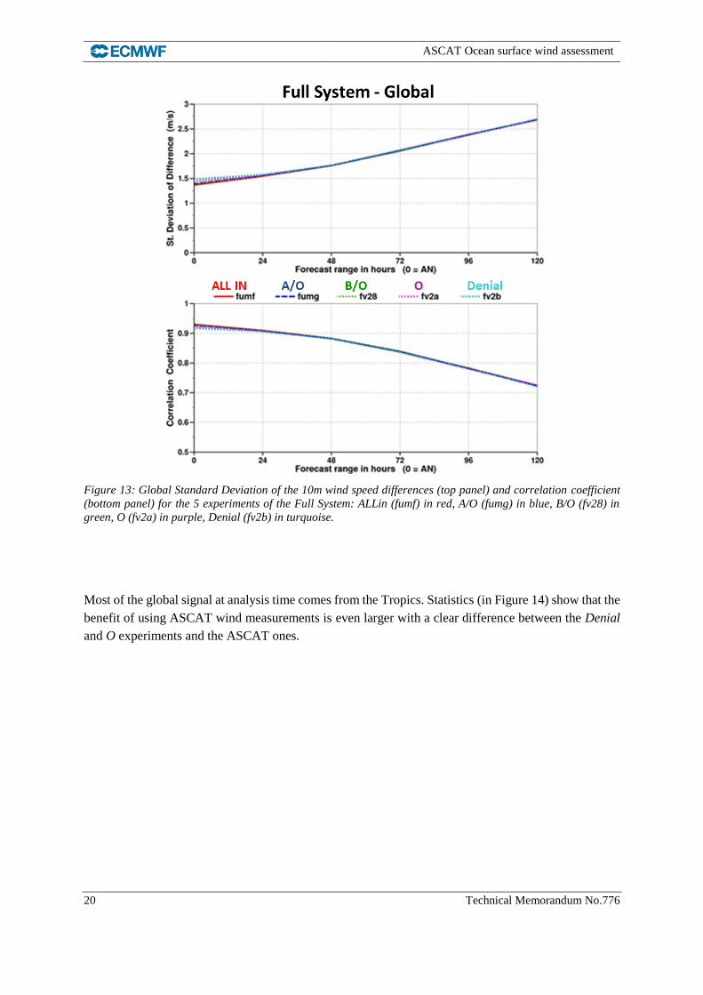
Figure 13: Global Standard Deviation of the 10m wind speed differences (top panel) and correlation coefficient
(bottom panel) for the 5 experiments of the Full System: ALLin (fumf) in red, A/O (fumg) in blue, B/O (fv28) in
green, O (fv2a) in purple, Denial (fv2b) in turquoise.
Most of the global signal at analysis time comes from the Tropics. Statistics (in Figure 14) show that the
benefit of using ASCAT wind measurements is even larger with a clear difference between the Denial
and O experiments and the ASCAT ones.

ASCAT ocean surface wind assessment
Technical Memorandum No.776 21
Figure 14: Standard Deviation of the 10m wind speed differences (top panel) and correlation coefficient (bottom
panel) for the 5 experiments of the Full System in the Tropics: ALLin (fumf) in red, A/O (fumg) in blue, B/O (fv28)
in green, O (fv2a) in purple, Denial (fv2b) in turquoise.
For the Starved System (not shown here) the signals from the global and regional statistics are slightly
larger than for the Full System set of experiments. This is explained considering that with fewer
observations in the system the impact of all the scatterometer winds is larger. With this configuration a
positive impact is visible globally only at analysis time but in the Tropics a small benefit is shown also
for the 24h and 48h forecasts. These signals are even more evident for the Starved+ System set of
experiments (Figure 15). The benefit of assimilating either or both ASCAT datasets is much larger. The
positive impact of using scatterometer observations is shown not only in the analysis but also in the 24h
and 48h forecast where the Denial experiment has higher standard deviation and lower correlation
coefficient than the other experiments.

ASCAT Ocean surface wind assessment
22 Technical Memorandum No.776
Figure 15: Standard Deviation of the 10m wind speed differences (top panel) and correlation coefficient (bottom
panel) for the 5 experiments of the Starved+ System in the Tropics: ALLin (fx03) in red, A/O (fx02) in blue, B/O
(fxh0) in green, O (fxh5) in purple, Denial (fxh6) in turquoise.

ASCAT ocean surface wind assessment
Technical Memorandum No.776 23
4.3.1 Verification of single instrument experiments
In order to analyse the performances of each single instrument, in all the three scenarios, the experiments
assimilating respectively only ASCAT-A, ASCAT-B and OSCAT were compared to the Denial one.
The verification versus altimeter winds confirms that at analysis time even a single scatterometer is
beneficial. Morover ASCAT and OSCAT have similar impact in the Full System (Figure 16).
Figure 16: Standard Deviation of the 10m wind speed differences (top panel) and correlation coefficient (bottom
panel) for the experiments of the Full System in the Tropics: A (fumh) in red, B (fv29) in blue, O (fv2a) in green,
Denial (fv2b) in purple.
Similar results were found for the Starved System. In the Starved+ System the results confirm that the
impact of assimilating scatterometer winds is propagated further into the forecast, with detectable impact
out to 3-5 days (Figure 17).

ASCAT Ocean surface wind assessment
24 Technical Memorandum No.776
Figure 17: Standard Deviation of the 10m wind speed differences (top panel) and correlation coefficient (bottom
panel) for the experiments of the Starved+ System in the Tropics: A (fxh2) in red, B (fxh3) in blue, O (fxh5) in
black, Denial (fxh6) in green.
4.4 Verifications against buoy
The three groups of OSEs have been verified also against buoy observations. Wave and wind data from
moored buoys and platforms that are broadcast to the meteorological community through the Global
Telecommunication System (GTS) have been used. Data quality control and scale matching procedures
were applied. Wind observations, which are assimilated in the atmospheric model, are corrected to a 10
m height. The wave observations are not assimilated in the wave model therefore they can be considered
to some extent independent observations.
For the verification, buoy wind data have been used only in the tropics, whereas buoy wave data have
been used only in the extra-tropics. The number of wave observations from tropical buoys is indeed not
enough to give a clear picture of the Tropics. A map of the wave (in purple) and wind (in blue) buoys is
presented in Figure 18. Top panel shows the tropical buoys and it can be noticed that wave buoys are
mostly available only in the Central West Atlantic. The bottom panel shows the extra-tropical buoys.

ASCAT ocean surface wind assessment
Technical Memorandum No.776 25
Figure 18: map of tropical (top panel) and extra-tropical (bottom panel) buoys. Wave buoys are represented in
purple, wind ones in blue.
The global scatter index (SI - defined as the standard deviation of difference between the model and the
observations normalized by the buoy mean) has been computed for the significant wave height and the
10m wind speed for each experiment of the three systems.
Overall the differences among the five experiments are quite small and they are more remarkable at
analysis time for the wave data and in the short range for wind data. A clear signal is that the Denial
experiment has the highest SI (i.e. is less beneficial for the system); this is also evident in the Starved
System and Starved+ System. The ALLin experiment has on the contrary the lowest SI. Overall the
experiments assimilating at least one ASCAT dataset have better performances. Different patterns can
be also distinguished for the tropical buoys and extra-tropical buoys.
4.4.1 Full System
Wave height and wind speed scatter index, for the 5 experiments of the Full System, are shown in Figure
19. The wave height SI is very similar for the 5 experiments at analysis time. For 48 hour forecast the
experiments assimilating scatterometer wind observations have a slightly lower SI value than in the
Denial (in turquoise). Statistics for the tropical wind speed show a higher value of SI for the Denial and
O (Oscat only) experiments at analysis time while the experiments assimilating ASCAT wind data show
better performances with a lower SI. The forecast results are mixed but the SI for the Denial experiments
is always the highest.

ASCAT Ocean surface wind assessment
26 Technical Memorandum No.776
Figure 19: Comparison of ECMWF significant wave height (top panel) and 10m wind speed (bottom panel) with
buoy data in terms of scatter index for the Full System experiments. Wave height statistics are based on extra-
tropical buoys, wind speed statistics on tropical buoys.
4.4.2 Starved System
Verification against buoy data for the Starved System experiments is presented in Figure 20. Again wave
height statistics show that there are no differences among the five experiments at analysis time while
some differences could be seen for the 48 hour and 72 hour forecasts, with the experiment assimilating
ASCAT data again showing lower SI. The statistics for the tropical wind speed show that the Denial
experiment has higher SI at analysis time and in the forecast. Experiments assimilating ASCAT data
have the lowest SI index.
ASCAT ocean surface wind assessment
Technical Memorandum No.776 27
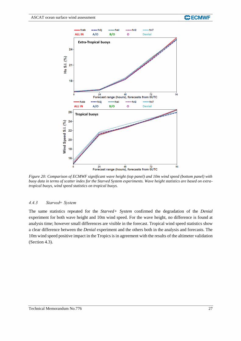
Figure 20: Comparison of ECMWF significant wave height (top panel) and 10m wind speed (bottom panel) with
buoy data in terms of scatter index for the Starved System experiments. Wave height statistics are based on extra-
tropical buoys, wind speed statistics on tropical buoys.
4.4.3 Starved+ System
The same statistics repeated for the Starved+ System confirmed the degradation of the Denial
experiment for both wave height and 10m wind speed. For the wave height, no difference is found at
analysis time; however small differences are visible in the forecast. Tropical wind speed statistics show
a clear difference between the Denial experiment and the others both in the analysis and forecasts. The
10m wind speed positive impact in the Tropics is in agreement with the results of the altimeter validation
(Section 4.3).

ASCAT Ocean surface wind assessment
28 Technical Memorandum No.776
Figure 21: Comparison of ECMWF significant wave height (top panel) and 10m wind speed (bottom panel) with
buoy data in terms of scatter index for the Starved+ System experiments. Wave height statistics are based on extra-
tropical buoys, wind speed statistics on tropical buoys.
5 Collocation with Altimeter winds
Another assessment of the scatterometer winds has been done by collocating winds from the three
sensors (ASCAT-A, ASCAT-B, OSCAT) versus Altimeter winds from the Jason-1 satellite. Assimilated
scatterometer wind speed observations (thus after the bias correction is applied) from the ALLin
experiment of the Full System (fumf) have been collocated with Jason-1 winds (from super-observations
as described in Section 4.3). Scatterometer and altimeter observations acquired within 100 km and 100
minutes have been selected. Global statistics show that overall scatterometer winds are 0.2 m/s weaker
than Jason-1 winds, with ASCAT-B having the highest bias (0.24 m/s). Collocation of Jason-1 winds
versus ECMWF background (not shown here) shows however that altimeter winds are globally 0.37 m/s
stronger than the model over the period analysed.
Regional statistics (Table 4) show that the higher bias between scatterometer and Jason-1 winds is in
the Northern Hemisphere (ASCAT-A 0.24 m/s, ASCAT-B 0.38 m/s, OSCAT 0.42 m/s) where also
Jason-1 has the highest bias compared to ECMWF background winds. The lowest bias is seen in the

ASCAT ocean surface wind assessment
Technical Memorandum No.776 29
Southern Hemisphere (ASCAT-A 0.12 m/s, ASCAT-B 0.18 m/s, OSCAT 0.16 m/s). Analysis of the
regional plots does not show any particular patterns in the data.
Figure 22: Scatterometer winds versus Jason-1 winds. Top left panel is for ASCAT-A winds, top right panel for
ASCAT-B and bottom panel for OSCAT.
Global NH Tropics SH
ASCAT-A -0.21 -0.24 -0.2 -0.12
ASCAT-B -0.24 -0.38 -0.26 -0.18
OSCAT -0.19 -0.42 -0.11 -0.16
Table 4: Global and regional wind speed bias between scatterometer and Jason.

ASCAT Ocean surface wind assessment
30 Technical Memorandum No.776
6 Forecast Error Sensitivity to Observations
The impact of scatterometer winds on the different systems has also been evaluated using the Forecast
error Sensitivity to Observations Impact technique (FSOI) which is an adjoint-based diagnostics to
estimate the forecast sensitivity to individual observations (Cardinali, 2009). The tool computes the
contribution of all observations to the forecast error (Forecast Error Contribution - FEC): a positive
contribution is associated with forecast error increase and a negative contribution with forecast error
decrease. The forecast range investigated is 24 hour. FSOI and OSEs measure different aspects of
forecast impact: OSEs provide occasional but comprehensive analysis of the observation impact on
meteorological fields; FSOI provides a routine analysis but for a particular target metric (e.g. the global
dry energy norm, which depends on wind, temperature and surface pressure, of the 24 hour forecast);
the FSOI (adjoint-based technique) is restricted by the tangent linear assumption and is therefore valid
only for forecasts up to one day, while OSE can measure the data impact on longer range forecast and
in nonlinear regimes.
The forecast impact, or Forecast Error Contribution (FEC), depends on the forecast error, the
assimilation system and the difference between the observations and the model. However the results
should be interpreted with care, as the diagnostic is based on evaluating forecast error through a
comparison to analyses, and for 24h forecast ranges analysis errors can significantly contribute to the
apparent forecast errors in such a comparison. This problem also occurs in classical observing system
experiments, as discussed in Section 5, for which short-range verification scores can crucially depend
on the choice of verifying analysis. The FEC, computed as percentage over the whole set of
observations, has been computed for each type of observation assimilated in the three systems analysed.
A global statistics has been computed as well as regional ones for the Northern Hemisphere, Tropics
and Southern Hemisphere. The statistics have been also stratified for each scatterometer datasets. Since
AMSU-A observations are the ones with most impact on the system, the FEC for each AMSU-A dataset
has also been calculated.
6.1 Full System
For the Full System, statistics (Figure 23) show that the FEC for scatterometer observations is about
7.5% when they are all assimilated (ALLin experiment), around 7% when either ASCAT-A or ASCAT-
B are assimilated with OSCAT and about 6% when only OSCAT is assimilated. The higher impact of
OSCAT, compared to ASCAT, is due to higher number of observations assimilated. As expected
AMSU-A has the higher impact in the reduction of the forecast error with a FEC of about 22.5%. When
no scatterometer observations are assimilated (Denial experiment) AMSU-A FEC reaches about 25%.
The other observations that gain impact are IASI, AMVs and AIREP, all wind observations.

ASCAT ocean surface wind assessment
Technical Memorandum No.776 31
Figure 23: Global total forecast error contribution (in percentage) grouped by observation type for the Full System
over the period 17 December 2012-28 February 2013. The error bars are computed using the standard deviation
of the forecast error.
Statistics have also been computed for the Northern Hemisphere, Tropics and Southern Hemisphere. As
shown in Figure 24, Figure 25 and
Figure 26, scatterometer impact is slightly lower in the Northern Hemisphere and Tropics with a FEC
of about 6% when all the observations are assimilated, but is higher in the Southern Hemisphere with a
FEC of about 10%. Compared to the global statistics, overall in the Northern Hemisphere (Figure 24)
the conventional observations have a higher impact, particularly Aircraft Measurements (AIREP). In
the Tropics (Figure 25) a large increase can be noticed for AMVs impact. While in the Southern
Hemisphere the increase is largest for AMSU-A, scatterometer and IASI.
0 5 10 15 20 25 30
SYNOPAIREPDRIBUTEMPDROPPILOT
PROFILERAMVsSCATHIRS
AMSU-AATMSAIRSIASI
GPS-ROMHS
AMSU-BGeosat-Rad
GBRADALLSKY-SSMISALLSKY-TMI
FEC % - Full System - Global
ALLin
A/O
B/O
O
Den

ASCAT Ocean surface wind assessment
32 Technical Memorandum No.776
Figure 24: Total forecast error contribution (in percentage) grouped by observation type for the Full System over
the period 17 December 2012-28 February 2013 in the Northern Hemisphere.
Figure 25: Total forecast error contribution (in percentage) grouped by observation type for the Full System over
the period 17 December 2012-28 February 2013 in the Tropics.
0 5 10 15 20 25 30
SYNOPAIREPDRIBUTEMPDROPPILOT
PROFILERAMVsSCATHIRS
AMSU-AATMSAIRSIASI
GPS-ROMHS
AMSU-BGeosat-Rad
GBRADALLSKY-SSMISALLSKY-TMI
FEC (%) - Full System - Northern Hemisphere
ALLin
A/O
B/O
O
Denial
0 5 10 15 20 25 30
SYNOPAIREPDRIBUTEMPDROPPILOTAMVsSCATHIRS
AMSU-AATMSAIRSIASI
GPS-ROMHS
AMSU-BGeosat-Rad
ALLSKY-SSMISALLSKY-TMI
FEC (%) - Full System - Tropics
ALLin
A/O
B/O
O
Denial

ASCAT ocean surface wind assessment
Technical Memorandum No.776 33
Figure 26: Total forecast error contribution (in percentage) grouped by observation type for the Full System over
the period 17 December 2012-28 February 2013 in the Southern Hemisphere.
To verify also the impact of each single sensor, the statistics have been computed for each scatterometer
and AMSU-A sensor (Figure 27). Among the scatterometers, OSCAT has the highest impact FEC:
3.5% when all the scatterometer observations are assimilated. This value rises to 5.5% when only
OSCAT is assimilated. ASCAT-A and ASCAT-B have similar impact: 2% when they are both
assimilated and 2.5% if only one of them is used. METOP-B AMSU-A has the highest impact among
the AMSU-A sensors with a FEC of about 5.5%. AMSU-A on board satellite NOAA-18 and NOAA-19
have similar impact, around 4.5%. METOP-A AMSU-A has slightly lower impact; this may be due to
the loss of channel 7 which is believed to be important. Regional statistics (not shown here) indicate that
these results are similar in all regions.
Results of FEC per observation each single scatterometer dataset are shown in Figure 28 (left-hand
panel) where the total forecast error contribution is normalized for the number of observations. ASCAT-
A and ASCAT-B observations have the highest FEC when either of them is used.
0 5 10 15 20 25 30
SYNOP
AIREP
DRIBU
TEMP
PILOT
AMVs
SCAT
HIRS
AMSU-A
ATMS
AIRS
IASI
GPS-RO
MHS
AMSU-B
Geosat-Rad
ALLSKY-SSMIS
ALLSKY-TMIFEC (%) - Full System - Southern Hemisphere
ALLin
A/O
B/O
O
Denial

ASCAT Ocean surface wind assessment
34 Technical Memorandum No.776
Figure 27: Global total forecast error contribution (in percentage) for Scatterometer and AMSU-A sensors for the
Full System over the period 17 December 2012-28 February 2013.
Figure 28: Average forecast error contribution (left-hand panel) and number of observations assimilated (right-
hand panel) for ASCAT-A, ASCAT-B and OSCAT over the period 17 December 2012-28 February 2013.
6.2 Starved System
When other satellite observations, which are sources of wind information, are removed from the GOS
(Starved System) the impact is redistributed mostly over the AMSU-A, scatterometer and AIREP
observations (Figure 29). Scatterometer FEC reaches about 10% and AMSU-A about 25% for the ALLin
experiment. When also scatterometer observations are removed (Denial experiment) AMSU-A impact
is about 28%.
6.3 Starved+ System
When AMSU-A observations are removed from the GOS (Starved+ System), all the other observations
increase their impact (Figure 30). The largest changes are for IASI, AIRS and scatterometer, for which
FEC is doubled. Scatterometer impact is 12% when all the scatterometer observations are assimilated
(ALLin experiment).
0 1 2 3 4 5 6 7
ASCAT-A
ASCAT-B
OSCAT
AMSU-A/MetopB
AMSU-A/MetopA
AMSU-A/AQUA
AMSU-A/A-15
AMSU-A/A-18
AMSU-A/A-19FEC % - Full System - Global
ALLin
A/O
B/O
O
Den
-0.3 -0.2 -0.1 0
ASCAT-A
ASCAT-B
OSCAT
FEC (J) x single obsALLin
A/O
B/O
O
0 50 100 150 200
ASCAT-A
ASCAT-B
OSCAT
N. Observations (x 100000)
ALLin
A/O
B/O
O

ASCAT ocean surface wind assessment
Technical Memorandum No.776 35
Figure 29: Global total forecast error contribution (in percentage) grouped by observation type for the Starved
System over the period 17 December 2012-28 February 2013.
Figure 30: Global total forecast error contribution (in percentage) grouped by observation type for the Starved+
System over the period 17 December 2012-28 February 2013.
0 5 10 15 20 25 30
SYNOP
AIREP
DRIBU
TEMP
DROP
PILOT
PROFILER
SCAT
HIRS
AMSU-A
ATMS
AIRS
IASI
GPS-RO
MHS
AMSU-B
GBRAD FEC % - StarvSys - Global
ALLin
A/O
B/O
O
Den
0 5 10 15 20 25 30
SYNOP
AIREP
DRIBU
TEMP
DROP
PILOT
PROFILER
SCAT
HIRS
ATMS
AIRS
IASI
GPS-RO
MHS
AMSU-B
GBRADFEC % - StarvSys Plus - Global
ALLin
A/O
B/O
O
Den

ASCAT Ocean surface wind assessment
36 Technical Memorandum No.776
7 Tropical Cyclones Verification
An analysis to verify the impact of scatterometer observations on Tropical Cyclones (TC) was
performed. For such extreme events it is preferable not to use scores and diagnostics normally used for
the verification of OSEs experiments. It is more appropriate to use scores that are representative of the
characteristics of a TC. The metrics identified and tested are the vertical wind shear, the mean sea level
pressure at the centre of the storm and position of the storm centre. The error of the storm position can
be split into the two components: along-track distance and across-track distance. The former is related
to the speed of the storm and suggests if the model is moving the storm too fast or too slow, the latter is
related to the ability of the model to change the trajectory of the storm.
An analysis on the impact of scatterometer winds assimilation on the errors in SLP and position of the
TC centre was performed. A tool developed at ECMWF (Vitart et al., 1997) which detects tropical
storms from ECMWF model fields, in particular the centre of a tropical storm and the related Sea Level
Pressure (SLP), was used for this study. To evaluate the impact of scatterometer observations on the
representation of these storms, the algorithm was run for all the experiments of the three systems (Full
System, Starved System, Starved+ System). For each day the position and the minimum SLP for each
tropical cyclone was detected both in the analysis and in the forecasts. For each storm and forecast step,
the position of the storm centre and the SLP centre have then been compared to the estimated value. The
estimated cyclone location and depth are received from the Regional Specialized Meteorological Centres
(RSMCs) recognized by WMO: they are the National Hurricane Center (NHC) for the North Atlantic
region and the Japan Meteorological Agency (JMA) for the West Pacific Region. These observations
are also known as Best Track (BT). To compute the mean errors, only the storms detected in all the
experiments have been used so that the number of cases analysed is the same. The number of cases used
to compute the statistics ranges from 31 (12h forecast range) to 14 (60h forecast range). Beyond 60h
forecast, the number of cases is considered too small to make any significant conclusions.
In Figure 31 the error (in millibar) between the observed minimum sea level pressure and the ECMWF
one is plotted for each experiment of the Full System (top-left panel), Starved System (top-right panel),
Starved+ System (bottom panel). There are not many differences among the experiments of the Full
System. For the Starved System and Starved+ System the difference among the experiments assimilating
scatterometer observations is negligible. However there is signal of a small increase of the error for the
Denial experiment in both systems. This is particularly consistent in the Starved+ System for all the
forecast steps. In Figure 32 the distance (in km) between the ECMWF forecasted TC position and the
observed one is presented for each experiment of the three systems. For this parameter it is not possible
to identify a pattern in the results; all the experiments show similar results.
The distance between the observed storm centre and the ECMWF forecasted one has been computed in
terms of the two components (across-track and along-track). This analysis (not shown here), does not
indicate any specific trend in the results. This investigation was based on all the tropical cyclones that
occurred during the period under investigations and detected by the automatic procedure.

ASCAT ocean surface wind assessment
Technical Memorandum No.776 37
Figure 31: Difference of the Sea Level Pressure at the centre of the storm difference between the ECMWF forecast
and Best Track observations for all the experiments of the Full System (top-left panel), Starved System (top right
panel) and Starved+ System (bottom panel).
Figure 32: Distance of the TC centre position (ECMWF Forecast - Observations) for all the experiments of the
Full System (top-left panel), Starved System (top right panel) and Starved+ System (bottom panel).

ASCAT Ocean surface wind assessment
38 Technical Memorandum No.776
The analysis was repeated by filtering only the TCs over which ASCAT-A, ASCAT-B and OSCAT
scatterometer observations were available at analysis time. This second analysis was repeated comparing
a different set of experiments. In Figure 33 Root Mean Square (RMS) forecast error (in hPa) between
the RMSC estimated minimum sea level pressure and the ECMWF one is plotted for different
experiments of the Full System assimilating different number of scatterometer datasets: ALLin in light
blue, A/B in red, O in green, Denial in purple. The experiments clearly show that ASCAT impact is
larger than OSCAT, but that the best result is achieved when all three scatterometers are assimilated.
Figure 33: Root mean square forecast error of the Sea Level Pressure at the centre of the TC for 12, 24 and 36
hour forecast step (in blue the ALLin experiment assimilating ASCAT-A, ASCAT-B and OSCAT data; in red the
A/B experiment assimilating ASCAT-A and ASCAT-B data; in green the O experiment assimilating only OSCAT
data, in purple the scatterometer Denial experiment).
In Figure 34 RMS forecast error (in Km), between the observed position of the storm centre and the one
retrieved from ECMWF model fields, is plotted for the different experiments. Overall, for all the forecast
steps analysed, the differences among the experiments are within 10km which is less that the model
resolution. Therefore, with such model resolution, the impact on the TC position is neutral.
This analysis has been repeated also selecting only passes where ASCAT-A and ASCAT-B only were
available, which included few more cases. Results (not shown here), confirm a clear benefit of
scatterometer wind assimilation on the MSLP forecast. While for the TC position, the error is still within
the model resolution.

ASCAT ocean surface wind assessment
Technical Memorandum No.776 39
Figure 34: Root mean square forecast error of the Sea Level Pressure at the centre of the TC for 12, 24 and 36
hour forecast step (in blue the ALLin experiment assimilating ASCAT-A, ASCAT-B and OSCAT data; in red the
A/B experiment assimilating ASCAT-A and ASCAT-B data; in green the O experiment assimilating only OSCAT
data, in purple the scatterometer Denial experiment).
7.1 New metrics for Tropical Cyclones: vertical wind shear
Besides SLP and tracking error, another parameter tested for the TC verification is the Vertical Wind
Shear (VWS). The VWS (the change of the wind with height) is a key factor that controls tropical
cyclogenesis and TC intensity: large values of VWS from the surface to the top of the troposphere are
generally detrimental to the formation as well as intensification of individual TCs. Observations and
numerical modelling studies show that strong VWS inhibits the development of incipient vortex and TC
intensification by weakening or destroying the organization of deep convection around the centre of the
storm.
TCs fill the entire vertical extent of the troposphere, and are driven by the average winds through this
layer. The VWS refers typically to the difference in wind speed between 200 hPa (the top of the
troposphere) and 850 hPa and is computed over a large area. VWS of less than 10 m/s are favourable
for tropical cyclone development. A weaker shear allows the storm to grow faster vertically into the air,
which helps the storm develop and become stronger. If the vertical shear is too strong, the TC can be
blown apart, since the mid-level warm core is displaced, and cannot rise to its full potential.
The 850hPa and 200hPa winds from the Full System experiments were used to compute the VWS in
this study. The analysis focused on the three active TC regions over the period of the experiments. In
Figure 35 the observed tracks of TC in the Eastern and Western Australian Basins and in the South-
West Indian Ocean are shown. First, the experiments ALLin and Denial have been compared. In Figure
36 the analysis difference between the two experiments (Denial-ALLin) is shown. Results based on more
than two months data do not show any particular signature in the areas of formation of the TCs. Similar
results are found when comparing other experiments or differences in RMS Forecast error (not shown
here). TCs are very strong events but localized in specific areas, therefore their signal is lost in long-
period averages. However repeating the analysis on shorter periods, such as few days over the TC

ASCAT Ocean surface wind assessment
40 Technical Memorandum No.776
genesis, did not show any specific pattern due to the averaging of the signal. The analysis of the VWS
over each 12 hour cycles showed a clear pattern. In Figure 37 the observed track of TC Felleng in the
South West Indian Ocean and in Figure 38, the VWS is shown for TC Felleng every 24 hours from 28
January 2013 00UTC to 2 February 2013. In each plot the observed position of the centre of the TC is
represented by a black diamond. The VWS is clearly low in the area of the TC centre and is surrounded
by an area with higher values; the VWS is also higher towards the end of the storm life when the storm
is weaker. Analysis differences of the VWS between Denial and ALLin experiments are shown in Figure
39.
Figure 35: TC observed tracks in the Eastern Australian Basin (top panel), Western Australian Basin (middle
panel) and South-West Indian Basin for the 2012-2013 season [MetOffice copyright].

ASCAT ocean surface wind assessment
Technical Memorandum No.776 41
Figure 36: Analysis Vertical Wind Shear differences between Denial and ALLin experiments over the South East
Indian basin (top panel) and South West Indian basin (bottom panel).
Figure 37: TC Felleng observation tracking from 28 January to 3 March 2013: each colour represents the strength
of the storm.

ASCAT Ocean surface wind assessment
42 Technical Memorandum No.776
Figure 38: Analysis Vertical Wind Shear for the ALLin experiment over the South West Indian basin for the TC
Felleng, every 24h from 20130128 00UTC to 20130202 00UTC. The black diamond represents the observed centre
of the storm.

ASCAT ocean surface wind assessment
Technical Memorandum No.776 43
Figure 39: Vertical Wind Shear analysis differences between Denial and ALLin experiments over the TC Felleng
every 24h from 20130128 00UTC to 20130202 00UTC. The black diamond represents the observed centre of the
storm.

ASCAT Ocean surface wind assessment
44 Technical Memorandum No.776
The differences between the two experiments show dipole patterns close to the TC centre, confirming
that the assimilation of scatterometer winds changes the structure of the storm. Overall it seems that the
ALLin experiment has lower VWS in the area towards which the storm was moved by the assimilation
of scatterometer data, which suggests that the assimilation of scatterometer data fosters the development
and the evolution of the storm.
7.2 Case Study: Typhon Haiyan
The Typhon Haiyan struck the Philippines on 8 November 2013 with winds of about 315 km/h and a
tremendous storm surge devastating a large portion of the Southeast Asia and killing more than 6000
people. It is considered to be the fourth strongest cyclone ever recorded, according to the Joint Typhoon
Warning Center (JTWC), and the strongest storm recorded at landfall. Haiyan originated from a low
pressure system in the Federated States of Micronesia on 2 November 2013 and then moved westward.
It became a storm with the name Haiyan on 4 November and soon reached the intensity of a Typhon by
18 UTC 5 November. On the 6 November the JTWC assessed the system as a Category-5 on the U.S.
Saffir-Simpson scale. The eye of the typhoon passed over the island of Kayangel, part of Palau. After
further intensification, Typhoon Haiyan hit central Philippines on 8 November with winds of 315 km/h
and gusts up to 370 km/h. Haiyan had a well-defined eye just before passing through the islands. The
storm then moved westward, gradually weakening, before emerging over the South China Sea. Turning
north westward, the typhoon eventually struck northern Vietnam as a severe tropical storm on November
10. Haiyan was last noted as a tropical depression by JMA the following day. The ECMWF deterministic
system forecast well the storm trajectory but the storm lacked intensity and strength both in the analysis
and forecasts. Reported central pressure was 895 hPa at 00 UTC on 8 November, in ECMWF analysis
it was much weaker, 966 hPa, which might in part be related to the small size of the cyclone. Clearly a
wrong central pressure leads to wrong wind speeds. In Figure 40 the minimum pressure is displayed
from the 5 November 2013 to 9 November 2013: in black is the estimated minimum pressure (from
‘best track’ - BT - files) and in red the ECMWF analysis and forecast minimum pressure. As can be
seen, the difference between the estimated minimum of the Sea Level Pressure (mSLP) and the ECMWF
one is quite large reaching almost 70 hPa on 7 November 06UTC. The uncertainty on the BT estimated
mSLP is high. But even considering this the difference with the ECMWF value is high. On 7 November
18UTC there is a large difference between the background (12h forecast) and the analysis (blue points)
with a difference of about 10 hPa indicating that something in the assimilation pushed the minimum
pressure up.
Partially the minimum pressure difference was due to the model resolution. Experiments run at ECMWF
at higher resolution showed that cyclone deepens earlier and the central pressure was deeper (up to
17hPa) than in operations.

ASCAT ocean surface wind assessment
Technical Memorandum No.776 45
Figure 40: Minimum sea level pressure over the Typhoon Haiyan from 5 November 2013 to 9 November 2013: in
black the observed minimum value, in red the minimum value from the operational mSLP forecast field: in light
red 6h and 12h forecast from the 06 analysis, in dark red the 6h and 12h forecast from the 18 analysis.
Although Haiyan is outside the period chosen for all the other experiments for this project, we
considered it to be a very good case study to better understand the role played by scatterometer wind
observations in the IFS system in such an extreme event and to investigate possible improvements in
the assimilation scheme. The investigation is particularly focused on the cycle of 7 November 2013
12UTC. In Figure 41, the assimilated ASCAT-A (red), ASCAT-B (green) and OSCAT (purple) winds
are shown for the cycle of 7 November 2013 12UTC (observations are acquired between 09UTC and
21UTC). The mean sea level pressure field is shown with the blue contour. The ASCAT-A and ASCAT-
B swaths did not fully cover the whole typhoon area. OSCAT covered only a small part of it, in part
because some observations were rejected due to the rain contamination in the typhoon eye area.
The analysis has focused on the impact of ASCAT-A winds. In Figure 42 the (best ambiguous) ASCAT-
A observed wind speed (left hand panel) and the background wind speed at the observation location
(right hand panel) are plotted for 7 November 2013 12UTC. According to ASCAT-A observations, the
typhoon is located slightly to the west of the position predicted in the background; the area of strongest
winds is also slightly smaller than the one expected from the background wind fields. For both datasets
the strongest wind speed in the area is around 33 m/s.
In Figure 43 only the actively assimilated ASCAT-A winds (left-hand panel) are plotted and the relevant
background wind values (right-hand panel). The less dense number of observations is due to the
thinning. Some ASCAT-A observations close to the eye of the storm have been rejected during the
assimilation. As part of the quality control, if the wind vector difference between the observation and
the background is too large the observations are rejected. In this case the rejection is due to the wind
direction difference between ASCAT-A and background; this is most likely due to the shift of the
position of the centre of the storm. This can be seen in Figure 44 where the mean background departure
(observation - background) is plotted in terms of vector wind differences. After having applied the
thinning and the quality control, the strongest ASCAT-A wind assimilated is around 25 m/s,
significantly lower than the maximum wind speed observed and the ECMWF background one. This
means than in the assimilation the ASCAT-A observations acted to reduce the analysis winds.

ASCAT Ocean surface wind assessment
46 Technical Memorandum No.776
Figure 41: Scatterometer wind observations assimilated on 7 November 2013 over the typhoon Haiyan: ASCAT-
A in red, ASCAT-B in green, OSCAT in purple.
Figure 42: All ASCAT-A observed wind speed (left hand panel) and the background wind speed at the observation
location (right hand panel) are plotted for the cycle 7 November 2013 12UTC.

ASCAT ocean surface wind assessment
Technical Memorandum No.776 47
Figure 43: Assimilated ASCAT-A wind speed (left hand panel) and the background wind speed at the observation
location (right hand panel) are plotted for the cycle 7 November 2013 12UTC.
Figure 44: Mean background departure (all ASCAT-A - ECMWF background) for the 10m vector wind difference
for the cycle 7 November 12 UTC.
A zoom on the typhoon centre with ASCAT-A winds (arrows) and ECMWF analysis winds (shaded
colours) for 7 November 2013 12UTC is shown in Figure 45.
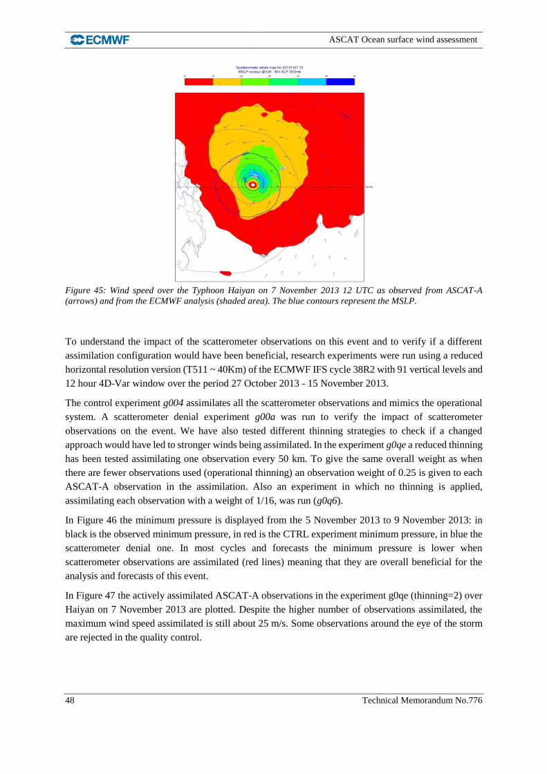
ASCAT Ocean surface wind assessment
48 Technical Memorandum No.776
Figure 45: Wind speed over the Typhoon Haiyan on 7 November 2013 12 UTC as observed from ASCAT-A
(arrows) and from the ECMWF analysis (shaded area). The blue contours represent the MSLP.
To understand the impact of the scatterometer observations on this event and to verify if a different
assimilation configuration would have been beneficial, research experiments were run using a reduced
horizontal resolution version (T511 ~ 40Km) of the ECMWF IFS cycle 38R2 with 91 vertical levels and
12 hour 4D-Var window over the period 27 October 2013 - 15 November 2013.
The control experiment g004 assimilates all the scatterometer observations and mimics the operational
system. A scatterometer denial experiment g00a was run to verify the impact of scatterometer
observations on the event. We have also tested different thinning strategies to check if a changed
approach would have led to stronger winds being assimilated. In the experiment g0qe a reduced thinning
has been tested assimilating one observation every 50 km. To give the same overall weight as when
there are fewer observations used (operational thinning) an observation weight of 0.25 is given to each
ASCAT-A observation in the assimilation. Also an experiment in which no thinning is applied,
assimilating each observation with a weight of 1/16, was run (g0q6).
In Figure 46 the minimum pressure is displayed from the 5 November 2013 to 9 November 2013: in
black is the observed minimum pressure, in red is the CTRL experiment minimum pressure, in blue the
scatterometer denial one. In most cycles and forecasts the minimum pressure is lower when
scatterometer observations are assimilated (red lines) meaning that they are overall beneficial for the
analysis and forecasts of this event.
In Figure 47 the actively assimilated ASCAT-A observations in the experiment g0qe (thinning=2) over
Haiyan on 7 November 2013 are plotted. Despite the higher number of observations assimilated, the
maximum wind speed assimilated is still about 25 m/s. Some observations around the eye of the storm
are rejected in the quality control.

ASCAT ocean surface wind assessment
Technical Memorandum No.776 49
Figure 46: Minimum sea level pressure over the Typhoon Haiyan from 5 November 2013 to 9 November 2013: in
black the observed minimum value, in red the minimum from the experiment g004 (control), in blue the value from
the experiment g00a (scatterometer denial).
Figure 47: ASCAT-A wind speed from the experiment g0qe (thinning=2 and observation weight = 0.025).
In Figure 48 the actively assimilated ASCAT-A observations in the experiment g0q6 (no thinning) over
Haiyan on 7 November 2013 are shown. In this case observations close to the eye of the storm are still
rejected but the highest wind speed assimilated is about 28 m/s, which is closer to the analysis wind
speed. These results suggest that there is a need to perform a deeper investigation on the thinning
strategies not only for the extreme events but also considering the general impact of scatterometer
observations on the ECMWF analysis and forecasts.

ASCAT Ocean surface wind assessment
50 Technical Memorandum No.776
Figure 48: ASCAT-A wind speed from the experiment g0q6 (no thinning).
7.3 Case Study: TC Norbert
The analysis performed on the TC Haiyan were repeated for the TC Norbert that hit the West Coast of
Mexico in September 2014. It was the major hurricane of the 2014 Pacific hurricane season. Norbert
originated from an area of low pressure on 2nd September. It moved north-westward reaching a hurricane
intensity on 4th September. On the 5th it reached Category 2 hurricane strength and continued deepening
reaching a peak of intensity on the 6th September with winds of 195 Km/h and a minimum SLP of about
960 hPa.
The reason for selecting this TC is that, like for Haiyan, some of the strongest observations of ASCAT-
A and ASCAT-B (the only sensors available at that time) close to the centre of the storm were rejected
by the Variational Quality Control (VarQC). In Figure 49 the assimilated ASCAT-A (red) and ASCAT-
B (green) winds are shown for the cycle of 6 September 2014 00UTC (observations are acquired
between 04UTC and 06UTC). The mean sea level pressure field is shown with the blue contour.
ASCAT-A and ASCAT-B swaths covered more than half of the TC area. The observations were
assimilated near the centre of the storm.
Following the outcome of the previous tests on the TC Haiyan, it was decided to run some experiments
changing both the thinning and the settings of the VarQC and verify how they affect the strongest wind
observation assimilated. The research experiments were run using a reduced horizontal resolution
version (T511 ~ 40Km) of the ECMWF IFS cycle 40R1 with 137 vertical levels and 12 hour 4D-Var
window for the cycle 6 September 2014. The control experiment g75r assimilates all the scatterometer
observations and mimics the operational system, g7c4 has a reduced thinning (one observation out of
two was assimilated), and another g75u without any thinning applied, which means that all the
observations were assimilated. Another set of experiments was run with the VarQC set to off: g755 with
standard thinning, g7c5 with reduced thinning, g75v without thinning.

ASCAT ocean surface wind assessment
Technical Memorandum No.776 51
Figure 49: Scatterometer wind observations assimilated on 6 September 2014 over the TC Norbert in the East
Pacific Ocean: ASCAT-A in red, ASCAT-B in green.
In
Figure 50 the actively assimilated ASCAT-A observations overt the TC Norbert for the 6 September
2014 are shown for a range of configurations. In the CTRL experiment (top-left panel), the strongest
assimilated wind in the area of the TC is about 17 m/s. When the VarQC is switched off (top-right) or
the thinning is reduced to one observation out of two (middle-left panel) the strongest wind is only 18
m/s because some strong winds are still rejected. When the thinning is reduced and the VarQC is off
(middle-right panel) the strongest wind is about 23 m/s. If the thinning is completely removed, the
strongest observation is around 22 m/s and 26 m/s, respectively with and without VarQC (bottom left
and bottom-right panels).
The differences in MSLP in the area of the centre of the storm for each of the above experiments has
been analysed. Overall the difference is quite small, within 2hPa. In terms of analysis maximum wind
speed, the maximum ASCAT wind speed assimilated varies in a range of about 10 m/s (from 18 to 26
for ASCAT-A, from 17 to 27 for ASCAT-B). This variability is reflected in a variability of the analysis
maximum wind speed of about 1.5 m/s (see Figure 51).
Overall this part of the study suggested that further investigations need to be performed in order to
improve the assimilation of high wind speeds. This will be of high importance when EPS-SG
scatterometer data, which will provide higher winds, is available. A preliminary analysis on a different
set-up of the Huber Norm and the thinning has been already performed but this needs to be tested more
extensively.

ASCAT Ocean surface wind assessment
52 Technical Memorandum No.776
Figure 50: Scatterometer wind observations assimilated on 6 September 2014 over the TC Norbert in the East
Pacific Ocean for the following experiments: g75r (CTRL), g75s(No VarQC), g75u(No Thinning), g75v(No VarQc
& No Thinning), g7c4(Thinning=2), g7c5 (Thinning=2 & No VarQC).
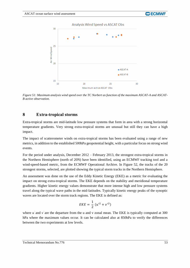
ASCAT ocean surface wind assessment
Technical Memorandum No.776 53
Figure 51: Maximum analysis wind speed over the TC Norbert as function of the maximum ASCAT-A and ASCAT-
B active observation.
8 Extra-tropical storms
Extra-tropical storms are mid-latitude low pressure systems that form in area with a strong horizontal
temperature gradients. Very strong extra-tropical storms are unusual but still they can have a high
impact.
The impact of scatterometer winds on extra-tropical storms has been evaluated using a range of new
metrics, in addition to the established 500hPa geopotential height, with a particular focus on strong wind
events.
For the period under analysis, December 2012 – February 2013, the strongest extra-tropical storms in
the Northern Hemisphere (north of 20N) have been identified, using an ECMWF tracking tool and a
wind-speed-based metric, from the ECMWF Operational Archive. In Figure 52, the tracks of the 20
strongest storms, selected, are plotted showing the typical storm tracks in the Northern Hemisphere.
An assessment was done on the use of the Eddy Kinetic Energy (EKE) as a metric for evaluating the
impact on strong extra-tropical storms. The EKE depends on the stability and meridional temperature
gradients. Higher kinetic energy values demonstrate that more intense high and low pressure systems
travel along the typical wave paths in the mid-latitudes. Typically kinetic energy peaks of the synoptic
waves are located over the storm track regions. The EKE is defined as:
𝐸𝐾𝐸 = 1
2 (𝑢′2 + 𝑣′2)
where u’ and v’ are the departure from the u and v zonal mean. The EKE is typically computed at 300
hPa where the maximum values occur. It can be calculated also at 850hPa to verify the differences
between the two experiments at low levels.

ASCAT Ocean surface wind assessment
54 Technical Memorandum No.776
Figure 52: Tracks of the 20 strongest Extra-Tropical Cyclones in the Northern Hemisphere (north of 20 N) for the
period 18 December 2012 – 28 February 2013.
In Figure 53 and 54 the differences of the mean EKE analysis at, respectively, 300 hPa and 850 hPa in
the Northern Hemisphere between the ALLin and Denial experiments of the Full System are shown. At
300 hPa none of the experiments seem to have a clear EKE signal even if on average the ALLin EKE is
slightly larger. At 850 hPa, the differences are more enhanced; in particular in the North Pacific storm
track area, the experiment assimilating scatterometer observations has larger EKE values than the Denial
one. This means that the assimilation, on average, intensifies the energy and the strength of the storms.
We have also tried to track extra-tropical storms using the EKE. The EKE has been computed for each
12 hour cycle over the lifetime of few selected storms; to capture the high-frequency signal from the
storms we have removed the 7 days running mean from the EKE. In Figure 55 the 300 hPa EKE anomaly
for the ALLin experiment is shown for an extra-tropical storm in the North Pacific Ocean every 12 hours
from 30 December 2012 00UTC to 1 January 2013 12UTC. The position of the storm has been detected
using the ECMWF tracking tool; the white triangular represent the position of the strongest wind in the
storm. In the pictures we can see the evolution of the EKE along the storm track with maximum values
of EKE (and wind speed) on the 31 December. This parameter gives an indication of the intensity and
structure of the storm but it does not help in identifying the centre of the storm.
In Figure 56 the map of the 300 hPa EKE anomaly differences between ALLin and Denial is shown
every 12 hours from 30 December 2012 00UTC to 1 January 2013 12UTC. We can identify dipole
patterns close to the storm area, confirming the assimilation of scatterometer winds changes the structure

ASCAT ocean surface wind assessment
Technical Memorandum No.776 55
of the storm. Overall the ALLin experiment has higher EKE (yellow-reddish colours) than the Denial
experiment confirming that the assimilation of scatterometer data intensify the strength of the storms.
Figure 53: Map of 300 hPa EKE analysis differences in the Northern Hemisphere between ALLin and Denial
experiments (Full System).
Figure 54: Map of 850 hPa EKE analysis differences in the Northern Hemisphere between ALLin and Denial
experiments (Full System).

ASCAT Ocean surface wind assessment
56 Technical Memorandum No.776
Figure 55: Map of 300 hPa EKE anomaly for the ALLin experiment from 30 December 2012 00UTC to 1 January
2013 12UTC for an extra-tropical storm in the North Pacific Ocean. The white triangular represents the estimated
position of the strongest high wind speed in the storm (derived using the ECMWF tracking tool as shown in Figure
52).

ASCAT ocean surface wind assessment
Technical Memorandum No.776 57
Figure 56: Map of 300 hPa EKE anomaly differences between ALLin and Denial experiments from 30 December
2012 00UTC to 1 January 2013 12UTC for an extra-tropical storm in the North Pacific Ocean. The white
triangular represents the estimated position of the strongest high wind speed in the storm (derived using the
ECMWF tracking tool as shown in Figure 52).
9 Surface Stress
Surface fluxes are important parameters in NWP. They are computed in the analysis and forecast
processes, generating several output products such as momentum flux, heat flux and fresh water flux.

ASCAT Ocean surface wind assessment
58 Technical Memorandum No.776
Among them, in a coupled system such as the ECMWF one, the momentum flux is the most relevant
since it is used as main forcing in the wave model and the ocean model. The accuracy of these fluxes is
therefore important for the performances of the atmospheric model but also for its feedback into the
ocean and wave models.
The momentum flux from the atmosphere into the ocean, also called surface stress, is computed in the
IFS from the Atmospheric model. The surface stress, τ, is defined as:
𝜏 = 𝜌 𝐶𝐷 |𝑢10|𝑢10
where CD is a dimensionless drag coefficient, ρ is the surface air density, u10 the 10 m wind.
Since scatterometer radar cross section is a function of the surface roughness and it is related to the
surface stress, we expect that these observations have a strong impact on this parameter. To verify this,
results from some experiments of the Full System were analysed. For each experiment the average over
six hours of the background Surface Stress (N/m2) has been considered. In Figure 57 the background
difference between the ALLin and the Denial experiments is shown.
Figure 57: Map of background differences in Averaged accumulated surface stress between ALLin and Denial
experiments.
The neutral wind speed, which is strongly connected to the surface stress, for the two experiments has
been compared (Figure 58).
Although the differences in wind speed show patterns similar to the ones in surface stress, in some areas
the impact of scatterometer winds seems to be different on the two parameters. For example, the impact
of assimilating scatterometer winds seems to be stronger in the North Atlantic than in the Tropical
Atlantic in terms of surface stress but lower in terms of neutral winds. These different patterns will be
further investigated in the follow-on study.
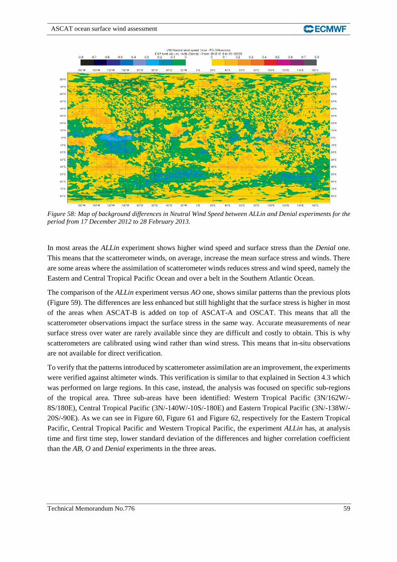
ASCAT ocean surface wind assessment
Technical Memorandum No.776 59
Figure 58: Map of background differences in Neutral Wind Speed between ALLin and Denial experiments for the
period from 17 December 2012 to 28 February 2013.
In most areas the ALLin experiment shows higher wind speed and surface stress than the Denial one.
This means that the scatterometer winds, on average, increase the mean surface stress and winds. There
are some areas where the assimilation of scatterometer winds reduces stress and wind speed, namely the
Eastern and Central Tropical Pacific Ocean and over a belt in the Southern Atlantic Ocean.
The comparison of the ALLin experiment versus AO one, shows similar patterns than the previous plots
(Figure 59). The differences are less enhanced but still highlight that the surface stress is higher in most
of the areas when ASCAT-B is added on top of ASCAT-A and OSCAT. This means that all the
scatterometer observations impact the surface stress in the same way. Accurate measurements of near
surface stress over water are rarely available since they are difficult and costly to obtain. This is why
scatterometers are calibrated using wind rather than wind stress. This means that in-situ observations
are not available for direct verification.
To verify that the patterns introduced by scatterometer assimilation are an improvement, the experiments
were verified against altimeter winds. This verification is similar to that explained in Section 4.3 which
was performed on large regions. In this case, instead, the analysis was focused on specific sub-regions
of the tropical area. Three sub-areas have been identified: Western Tropical Pacific (3N/162W/-
8S/180E), Central Tropical Pacific (3N/-140W/-10S/-180E) and Eastern Tropical Pacific (3N/-138W/-
20S/-90E). As we can see in Figure 60, Figure 61 and Figure 62, respectively for the Eastern Tropical
Pacific, Central Tropical Pacific and Western Tropical Pacific, the experiment ALLin has, at analysis
time and first time step, lower standard deviation of the differences and higher correlation coefficient
than the AB, O and Denial experiments in the three areas.

ASCAT Ocean surface wind assessment
60 Technical Memorandum No.776
Figure 59: Map of background differences in Surface Stress between ALLin and AO experiments for the period
from 17 December 2012 to 28 February 2013.
Figure 60: RMSE error and Correlation Coefficient for the experiments fumf (ALLin), fumi (AB), fv2a (O) and
fv2b (Denial) experiments for the period from 17 December 2012 to 28 February 2013 for the Eastern Tropical
Pacific.

ASCAT ocean surface wind assessment
Technical Memorandum No.776 61
Figure 61: RMSE error and Correlation Coefficient for the experiments fumf (ALLin), fumi (AB), fv2a (O) and
fv2b (Denial) experiments for the period from 17 December 2012 to 28 February 2013 for the Central Tropical
Pacific.
Figure 62: RMSE error and Correlation Coefficient for the experiments fumf (ALLin), fumi (AB), fv2a (O) and
fv2b (Denial) experiments for the period from 17 December 2012 to 28 February 2013 for the Western Tropical
Pacific.

ASCAT Ocean surface wind assessment
62 Technical Memorandum No.776
The experiments have been verified in the three areas using tropical buoy data. In Figure 63 and 64 the
wind speed Scatter Index (SI) are shown for the Eastern and Central Tropical Pacific. The experiment
assimilating all the observations (fumf - ALLin) has, at analysis time, lower SI than the one assimilating
only ASCAT-A and ASCAT-B, which is in turn lower than the O and Denial experiments. This result
confirms that in the region analysed the impact of the assimilation of scatterometer observations is
beneficial in terms of wind speed, and therefore also for surface stress. This is also in agreement with
the results in Section 4.4 showing that the benefit of scatterometer data is clear at analysis time but it is
not propagated in the mid-range forecast.
Figure 63: Comparison of ECMWF 10m wind speed with buoy data in terms of scatter index for the Full System
experiments fumf (ALLin), fumi (AB), fv2a (O) and fv2b (Denial) over the period from 17 December 2012 to 28
February 2013 for the North Eastern Tropical Pacific.
Figure 64: Comparison of ECMWF 10m wind speed with buoy data in terms of scatter index for the Full System
experiments fumf (ALLin), fumi (AB), fv2a (O) and fv2b (Denial) over the period from 17 December 2012 to 28
February 2013 for the Central Tropical Pacific.
To verify that the outcome of this analysis does not depend on surface stress seasonal variability, other
experiments were run over a summer period: g51b (ALLin) assimilating ASCAT-A, ASCAT-B and

ASCAT ocean surface wind assessment
Technical Memorandum No.776 63
OSCAT over the period from 1 June 2013 to 30 September 2013; g51c is scatterometer denial one
(NoScatt) over the same period. Also during the summer season, the pattern of the differences between
the experiments (Figure 65) is the same as the winter one, like seen in Figure 57 and Figure 58. This
means that the impact of the scatterometer observations on the surface stress does not depend on seasonal
surface stress trends. Since these experiments were run with a different IFS model cycle than the Full
System experiments, also the corresponding 'winter' experiments were run over the period from 17
December 2012 to 31 March 2013. Results, not shown here, confirm the same signal.
Figure 65: Map of background differences in Surface Stress between ALLin and AO experiments for the period
from 17 December 2012 to 28 February 2013.
10 Vertical Propagation of Scatterometer information
From the analysis of the impact of scatterometer observations, as seen in Section 4.1.1, it seems that
scatterometer observations have impact only up to 600 hPa; scatterometer assimilation appears to make
almost no difference above this height. It is known to be a common problem with all near surface
observations, especially wind, and might be due more to a weakness in the data assimilation system
rather than the observations themselves. However Leidner et al. (2003) showed that scatterometer wind
information was propagated up to about 200 hPa. The lower impact in the upper troposphere we find
may be due to the constraint imposed by the higher number of observations used compared to the Leidner
study. To verify the ability of 4D-var to propagate the scatterometer increments from the surface to
higher model levels, single observation experiments were run. This means that only one single
scatterometer wind observation is used. All the other observations, both conventional and from satellites,
are not assimilated. For this analysis the observation with the highest wind speed in the proximity of the
centre of Typhoon Haiyan for the cycle 2013110712 (with assimilation window from 9am to 9pm) has
been selected. The scatterometer observation has been acquired around 1pm, four hours after the
beginning of the assimilation window. Analysis at different model levels showed that the largest analysis
increments are found around 850 hPa. In Figure 66 the map of the SLP analysis increments for the cycle
07 November 2013 12 UTC in the area of the Typhoon Haiyan is shown. Each map displays the
increments every three hours from the beginning of the assimilation window. The maximum of the
increments occur after nine hours.

ASCAT Ocean surface wind assessment
64 Technical Memorandum No.776
Figure 66: Map of the MSLP analysis increments for the cycle 7 November 2013 12 UTC in the area of the Typhoon
Haiyan. Each map is for three hours since the beginning of the assimilation window (00h, 03h, 06h, 09h, 12h).
The analysis of the increments in terms of U and V also showed maximum values after nine hours from
the beginning of the assimilation window (Figure 67).

ASCAT ocean surface wind assessment
Technical Memorandum No.776 65
Figure 67: Map of the U-component analysis increments after 9H since the beginning of the assimilation window.
This is for the cycle 7 November 2013 12 UTC in the area of the Typhoon Haiyan.
Figure 68: Meridional Cross section across of the U-component (left-hand panel) and the V-component (right-
hand panel) analysis increments for the cycle 7 November 2013 12 UTC in the area of the Typhoon Haiyan.
The difference between the U and V components can be explained by the different background error
covariance (not shown here). For the cycle analysed, the background error covariance was larger for the
U-component which means that in the 4D-Var more weight was given to this parameter resulting in
larger increments.
In these experiments AMSU-A observations have the highest impact on the ECMWF system. To
investigate any possible interaction between scatterometer and AMSU-A data, observation experiments
with a horizontal resolution of T511 (~40km) have been run for the same date adding AMSU-A
observations to the scatterometer data. Different AMSU-A channels have been selected according to
their peak height. In one experiment the AMSU-A channels 5 and 6, which respectively peak at about
600 and 400 hPa, have been selected. The meridional cross-section along the maximum of the analysis
increments for the U component is presented in Figure 69: on the left the experiment assimilating only
one scatterometer observation, on the right the experiment assimilating also AMSU-A channels 5 and
6. The increments are slightly stronger when also AMSU-A observations are assimilated but the

ASCAT Ocean surface wind assessment
66 Technical Memorandum No.776
structure of the increments is very similar. Similar results were found for the V component (not shown
here).
Figure 69: Meridional Cross section across of the V-component analysis increments for the cycle 7 November
2013 12 UTC in the area of the Typhoon Haiyan for the experiment assimilating only one scatterometer
observation (left-hand panel) and the experiments assimilating one scatterometer observation and two AMSU-A
observations (channel 5 and channel 6).
To investigate any possible interaction at higher model level, two AMSU-A observations, channel 9 and
channel 10 which respectively peak around 100 and 50 hPa, have been assimilated with the scatterometer
one. Results in Figure 70 show that again the increments are slightly larger when also AMSU-A
observations are assimilated but, at low altitudes the structure is not modified. At higher model level
though we can notice a plume of increments at the height where the assimilated channels peak.
Figure 70: Meridional Cross section across of the V-component analysis increments for the cycle 07 November
2013 12 UTC in the area of the Typhoon Haiyan for the experiment assimilating only one scatterometer
observation (left-hand panel) and the experiments assimilating one scatterometer observation and two AMSU-A
observations (channel 9 and channel 10).
10.1 Test with an observation far from the TC
We showed above that if the observation is selected close to the centre of a TC it can have a high impact
on the analysis of the system. We then verified against the case of normal flow by selecting an ASCAT-
A observation far from the centre of the TC (1500km Nord-East), with a low/medium wind speed of
about 8.3 m/s and acquisition time at 11.21 a.m. (two hours after the beginning of the assimilation

ASCAT ocean surface wind assessment
Technical Memorandum No.776 67
window). The closest model grid wind speed was 8.5 m/s. As shown in Figure 71 and Figure 72, the
maximum of the MSLP and U/V wind components analysis increments was negligible close to the
observation location. A small analysis increments is seen in the area close to the TC (on the bottom left
of the figure) in the lower model levels after 9 and 12 hours from the beginning of the assimilation
window. Since the observation wind speed was very close to the model wind speed and therefore did
not have a great influence on the analysis, in this case, the increments were quite small.
Figure 71: Map of the MSLP analysis increments (cycle 07 November 2013 – 12 UTC) after 12H from the
beginning of the assimilation window.
Figure 72: Map of the V-component analysis increments at model level 137 (cycle 07 November 2013 – 12 UTC)
after 12H from the beginning of the assimilation window.
Other experiments were run adding AMSU-A observations to those from ASCAT-A. Results (not shown
here) confirmed that the analysis increments structure found when only one ASCAT-A observation is
assimilated is not strongly modified by the assimilation of one or two low or high AMSU-A channels.
10.2 Test with observations late in the assimilation window
We have seen before that the maximum of the analysis increments occurs in the assimilation window.
We verified the pattern of the analysis increments when the observation is acquired late in the
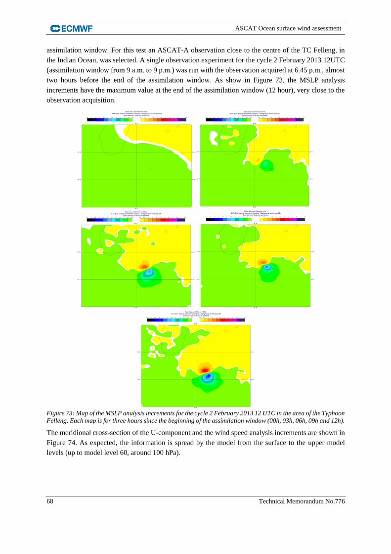
ASCAT Ocean surface wind assessment
68 Technical Memorandum No.776
assimilation window. For this test an ASCAT-A observation close to the centre of the TC Felleng, in
the Indian Ocean, was selected. A single observation experiment for the cycle 2 February 2013 12UTC
(assimilation window from 9 a.m. to 9 p.m.) was run with the observation acquired at 6.45 p.m., almost
two hours before the end of the assimilation window. As show in Figure 73, the MSLP analysis
increments have the maximum value at the end of the assimilation window (12 hour), very close to the
observation acquisition.
Figure 73: Map of the MSLP analysis increments for the cycle 2 February 2013 12 UTC in the area of the Typhoon
Felleng. Each map is for three hours since the beginning of the assimilation window (00h, 03h, 06h, 09h and 12h).
The meridional cross-section of the U-component and the wind speed analysis increments are shown in
Figure 74. As expected, the information is spread by the model from the surface to the upper model
levels (up to model level 60, around 100 hPa).

ASCAT ocean surface wind assessment
Technical Memorandum No.776 69
We have also repeated the test of adding AMSU-A observations (channels 5 and 6; channels 9 and10).
The meridional cross-section along the maximum of the analysis increments for the U component is
presented in Figure 75 and in Figure 76, respectively for the experiment assimilating ASCAT-A and
AMSU-A channels 5 and 6 and the experiment assimilating ASCAT-A and AMSU-A channels 9 and
10. Results show that in both cases the structure of the U-component analysis increments is not modified
when AMSU-A observations are added.
Figure 74: Meridional Cross section across of the U-component (left-hand panel) and wind speed (right hand
panel) analysis increments for the cycle 2 February 2013 12 UTC (after 12h) in the in the area of the Typhoon
Felleng.
Figure 75: Meridional Cross section across of the U-component analysis increments for the cycle 2 February
2013 12 UTC (at step 12h) in the in the area of the Typhoon Felleng for the experiment assimilating one ASCAT-
A observation and AMSU-A channel 5/6.

ASCAT Ocean surface wind assessment
70 Technical Memorandum No.776
Figure 76: Meridional Cross section across of the U-component analysis increments for the cycle 2 February
2013 12 UTC (at step 12h) in the in the area of the Typhoon Felleng for the experiment assimilating one ASCAT-
A observation and AMSU-A channel 9/10.
11 Conclusions
An extensive impact study of ASCAT winds on the ECMWF 4D-Var system was carried out in the
framework of the project between ECMWF and EUMETSAT “Support for ASCAT Ocean surface wind
assessment” (Project Ref. EUM/CO/12/4600001149/JF). The main aims of the project were the
evaluation of the current impact of scatterometer winds on the IFS analysis and forecast and the
optimization of the ASCAT winds assimilation strategy. The assimilation of ASCAT winds started in
2007 and its assimilation strategy has never been modified. During this time the IFS has evolved
considerably, in all aspects (model, assimilation, observations used). It is important to re-assess the
impact of scatterometer in the current IFS configuration. In this project, the impact has been evaluated
considering several aspects: impact on the analysis and forecast for different GOS scenarios; impact on
severe events such as Tropical Cyclones and extra-tropical storms; impact on the surface stress.
The impact of the ASCAT winds on the ECMWF 4D-Var system has been assessed for three different
GOS scenarios: one, Full system, is replicating the operational ECMWF system (at lower resolution)
and is using all the available observations; another scenario, Starved System, uses a subset of the GOS
(all observations except satellite observations that provide wind information); a third scenario, Starved+
System, from which also AMSU-A observations were removed together with satellite observations that
provide wind information. For each system, the impact of the scatterometer observations available at
the beginning of the project (ASCAT-A, ASCAT-B and OSCAT) have been assessed by running denial
experiments compared to a Control assimilating all the scatterometer data.
Different verification methods were used for the assessment: the main positive impacts are made when
either or both ASCAT datasets are assimilated together with OSCAT data. ASCAT-A and ASCAT-B
have a similar impact on the system to each other. Regional statistics show that overall the largest benefit
is coming from the Tropics. In the Full System configuration, the assimilation of scatterometer
observations is most beneficial at analysis time; this benefit does not in general propagate into the
forecast. Nevertheless, verifications against altimeter winds show that when other wind observations are

ASCAT ocean surface wind assessment
Technical Memorandum No.776 71
removed from the GOS, the positive impact at analysis time is larger and it also propagates to longer
forecast range. This suggests either some redundancy in surface wind information in the GOS or some
negative interaction between observation types in the data assimilation. The assimilation of ASCAT-B
winds has a positive impact on the analysis departure of ASCAT-A in all regions. It has a neutral to
positive impact on the analysis departure of OSCAT in the Northern Hemisphere and in the Tropics
while slightly increases it in the Southern Hemisphere. This is most likely due to the OSCAT wind speed
bias seen in the Southern Ocean (mostly south of 50 S), which is known and already partially corrected
by KNMI.
Forecast Error Contribution (FEC) statistics show that scatterometer observations used in the ECMWF
operational system contribute about 7.5% to the reduction of the 24-hour forecast error. OSCAT has a
higher impact than ASCAT winds; this is most likely due to the higher number of assimilated
observations. Statistics computed for each single observation show instead that a single ASCAT
observation has higher impact than a single OSCAT. ASCAT-A and ASCAT-B have the same impact.
Moreover, regional statistics show that the largest scatterometer observations impact comes from the
Southern Hemisphere.
The disagreement between the results of the verification versus altimeter winds (showing the main
impact in the Tropics) and FEC statistics (showing the main impact in the Southern Hemisphere) can be
explained by the differences of the two metrics. In the Tropics, Scatterometer observations have an
impact only close to the surface except for the in case of a TC, which are quite localized and not very
frequent phenomena; therefore in the Tropics a verification method using other surface wind
observations (like the case of altimeter data) is stronger than a metric based on an average over all model
levels (like the FEC). Conversely in the extra-tropics, where extra-tropical storms are quite frequent and
large scale phenomena, the impact of scatterometer on higher model levels is generally larger. In this
situation, the FEC statistics, based on a vertical average, are a more appropriate metric.
Verifications from the three systems showed that the impact of ASCAT winds is only propagated up to
600 hPa. A previous study (Leidener, 2003) showed that the impact was propagated up to 200 hPa.
Single observation experiments were run to verify if the 4D-Var is still able to propagate the
scatterometer wind information from the surface to the upper troposphere. Experiments assimilating one
scatterometer observation close to the centre of a TC showed that the impact is propagated up to 100
hPa. Similar experiments run with an observation far from the centre of the TC, in a less dynamic area,
showed that the analysis increment was very low. This is expected when the observation value is close
to the model value. Different tests have also been run to verify that the impact is propagated in time in
the assimilation window. To investigate the interaction between scatterometer observations and AMSU-
A, some experiments were run assimilating one scatterometer and up to two AMSU-A observations.
Results showed that the analysis increments structure at both high and lower levels is not significantly
modified when AMSU-A observations are assimilated. This suggests that the assimilation of AMSU-A
does not reduce the impact of ASCAT.
The impact of scatterometer wind observations on the TC forecast was also investigated. The RMS of
the minimum SLP forecast error in the centre of the storm is reduced when more scatterometer

ASCAT Ocean surface wind assessment
72 Technical Memorandum No.776
observations are assimilated confirming that they have a positive impact on these strong events. The
impact is neutral on the storm position forecast error.
Several TC case studies have been identified. The first one, on the Typhoon Haiyan, highlighted a
weakness in the assimilation strategy. It was noticed that some strong ASCAT winds in the area of
maximum storm intensity were rejected prior to the assimilation partially because of the thinning applied
(only one observation out of four is assimilated) and partially due to the Variational Quality Control
(VarQC). During the assimilation, differences between the observations and the background are
interpreted as observation error and the observations are therefore rejected. Sometimes this is not correct
since the observations can be more reliable than the background. In the cases analysed, ASCAT-A
observations were rejected in the area with stronger winds due to a displacement of the position of the
storm between scatterometer and the background. It can be considered that in a case like this,
scatterometer observations are more reliable in providing the position of the storm than the background
fields. These issues were found for other case studies of tropical cyclones. Several tests were then
performed by changing the thinning and the VarQC set-up. Stronger winds are assimilated when
reducing the thinning and lowering the VarQC thresholds. Despite some intense wind observations being
rejected during the VarQC, the analysis showed that overall the assimilation of scatterometer winds was
beneficial for the analysis and forecast of the Typhoon Haiyan.
The outcome from the TC analysis suggested to test and verify alternatives to the VarQC. The Huber
Norm seems to be a good candidate: it is a robust method which allows observations with large
background departure to still be given some weight in the data assimilation. Tests have been performed
and will be further investigated in a follow-on study. The thinning, especially in the case of TC, also
needs to be re-evaluated. Ideally, the thinning should be flow-dependent, so that when more observations
are needed the thinning can be reduced. This is because the observation error correlations are flow
dependent, due to representivity error. In such a complex system, like the ECMWF one, this is not
straightforward. Investigations on the feasibility of this change will be performed in the near future.
Alternative metrics for assessing the value of scatterometer have also been studied. Investigations on
the impact of the ASCAT winds on the extra-tropical cyclones using the Eddy Kinetic Energy at 300
hPa and 850 hPa showed that the assimilation of scatterometer observations has more impact at lower
model levels where it intensifies the storm structures, especially in the Northern Pacific Ocean. Further
investigations are needed to better characterize the impact. Scatterometer winds have showed to have
beneficial impact on the analysis and forecast of the surface stress. This is an important parameter,
computed in the atmospheric analysis and forecast and used as forcing for the wave and the ocean
models.
At ECMWF 25 Km ASCAT products have been assimilated since 2007. The ECMWF model resolution
was increased on March 9 2016 to 9 km, with consistent resolution increase in the data assimilation. The
use of ASCAT-A and ASCAT-B high resolution products should be re-evaluated in this system. In
preparation, the high resolution ASCAT products were tested to verify if they can be processed with the
current IFS configuration. Results were positive. Small changes are needed mostly related to the
computation of the σ0 and wind speed bias correction. Further assessment will be performed with the
new high resolution IFS configuration.

ASCAT ocean surface wind assessment
Technical Memorandum No.776 73
12 Acknowledgements
The first author acknowledges the funding provided through the EUMETSAT project “Support for
ASCAT Ocean surface wind assessment”. Thanks to Carla Cardinali for the explanations and the tool
to compute the FEC; to Saleh Abdalla for the support on the verification against altimeter winds;
Mohamed Dahoui, Linus Magnusson, Fernando Prates, Fredric Vittart and Tim Hewson for providing
tools and help related to TC and extra-TC analysis; Alan Geer for providing the IVER verification tool;
Hans Hersbach and Lars Isaksen for discussions on the scatterometer assimilation scheme and Huber
norm.
References
Andersson E, H. Jarvinen, 1999. Variational quality control. Q. J. R. Meteorol.Soc.125.
Bidlot, J.-R., D. J. Holmes, P.A. Wittmann, R. Lalbeharry, H.S. Chen, 2002. Intercomparison of the
performances of operational ocean wave forecasting systems with buoy data. Wea. Forecasting. 17. 287-
310.
Bidlot, J.-R. Extreme waves in the ECMWF operational wave forecasting system.
ftp://ftp.wmo.int/Documents/PublicWeb/amp/mmop/documents/JCOMM-TR/J-TR-34-9th-waves-
workshop/Papers/
Bidlot J, 2010. Use of Mercator surface currents in the ECMWF forecasting system. Research
Department Memorandum R60.9/JB/10104.
Bidlot J, 2012. Use of Mercator surface currents in the ECMWF forecasting system: a follow-up study.
Research Department Memorandum R60.9/JB/1228.
Bonavita M., L. Isaksen, E.V. Holm, 2012. On the use of EDA background error variances in the
ECMWF 4D-Var. Q. J. R. Meteorol. Soc.138, 1540–1559.
Bouttier, F., G. Kelly, 2001. Observing-system experiments in the ECMWF 4D-Var data assimilation
system. Q. J. R. Meteorol. Soc., 127 (574), 1469-1488. DOI: 10.1002/qj.49712757419.
Cardinali C., S. Pezzulli, E. Andersson, 2004. Influence-matrix diagnostic of a data assimilation system.
Q.J.R. Meteorol. Soc., 130, pp. 2767-2786.
Cardinali, C, 2009. Forecast sensitivity to observation (FSO) as a diagnostic tool, ECMWF Research
Department Technical Memorandum 599, ECMWF.
Cardinali C., 2013. Observation Impact on the Short Range Forecast. Lecture Notes from NWP Course,
ECMWF, June 2013.
De Chiara, G., P. Janssen, H. Hersbach, N. Bormann, 2012. Assimilation of scatterometer winds at
ECMWF. Proceedings of 11th International Winds Workshop, February 2012, Auckland, New Zealand.
De Chiara, G, 2012. Assimilation of OCEANSAT-2 Scatterometer winds. ECMWF Research Department
Memorandum, 2012, RD-63.
De Chiara, G., 2013. Preparation for the assimilation of ASCAT-B Scatterometer winds. ECMWF
Research Department Memorandum, RD13-294.
De Chiara, G., P. Janssen, S. English, J.-R. Bidlot and P. Laloyaux, 2014: Scatterometer Impact Studies
at ECMWF. Proceedings of the EUMETSAT Meteorological Satellite Conference 2014, September
2014, Geneva, Switzerland.

ASCAT Ocean surface wind assessment
74 Technical Memorandum No.776
De Maria, M., 1996. The effect of vertical shear on tropical cyclone intensity change. J. Atmos. Sci., 53,
2076-2087.
Figa Saldana, J., C. Anderson, 2012. ASCAT-B Validation and Calibration Report. EUMETSAT Report
EUM/OPS/DOC/12/3436.
Geer, A. J., P. Bauer and P. Lopez, 2010. Direct 4D-Var assimilation of all-sky radiances. Part II:
Assessment, Q. J. R. Meteorol. Soc., 136 (652), 1886-1905. DOI: 10.1002/qj.681.
Gray, W., 1968. Global view of the origin of tropical disturbances and storms. Mon. Wea. Rev., 96,
669–700.
Hersbach, H., 2007. Preparation for assimilation of surface-wind data from ASCAT at ECMWF.
ECMWF Research Department Memorandum R60.9/HH/0750.
Hersbach, H., 2008. CMOD5-N: A C-band geophysical model function for equivalent neutral wind.
ECMWF Technical Memorandum 554.
Hersbach H., 2010. Assimilation of scatterometer data as equivalent-neutral wind, ECMWF Tec. Memo
629.
Hersbach, H., and P. Janssen, 2007. Improved scatterometer screening. ECMWF Research Department
Memorandum R60.9/HH/0735.
Hersbach H. and J.R. Bidlot, 2008. The relevance of ocean surface current in the ECMWF analysis and
forecast system. Proceedings from the ECMWF Workshop on Atmosphere-Ocean Interaction, 10-12
November 2008. Available at ww.ecmwf.int/publications/library/do/references/list/28022009.
Leidner, S.M., L. Isaksen and R.N. Hoffman, 2003: Impact of NSCAT Winds on Tropical Cyclones in
the ECMWF 4DVAR Assimilation System. Mon. Weather Rev., 131, 3–26.
Stoffelen, A., 1999. A simple method for calibration of a scatterometer over the ocean. J. Atmos.
Oceanic Technol., 16, 275-282.
Tang, B., K. Emanuel, 2012. A Ventilation Index for tropical cyclones. Bull. Amer. Meteor. Soc., 93,
1901–1912.
Tavolato, C., L. Isaksen, 2014. On the use of a Huber norm for observation quality control in the
ECMWF 4D-Var Christina Tavolato. Q.J.R. Meteorol. Soc.. doi: 10.1002/qj.2440
Verhoef, A., A. Stoffelen, 2012. OSCAT winds validation report. Technical Note
SAF/OSI/CDOP2/KNMI/TEC/RP/196, EUMETSAT.
Vitart, F., J.J. Anderson, W.F. Stern, 1997. Simulation of Interannual Variability of Tropical Storm
Frequency in an Ensemble of GCM Integrations, Journal of Climate, vol 10, 745-760.
www.metoffice.gov.uk/weather/tropicalcyclone/observations