Incentives and Performance in the Presence of Wealth Effects and

Endogenous Risk

Ming Guo and Hui Ou-Yang∗

This Version: October 15, 2003

∗Guo is with the Department of Economics, Duke University, Durham, NC 27708. E-mail: mg22@duke.edu.Ou-Yang is with the Fuqua School of Business, Duke University, Durham, NC 27708-0120. E-mail: huiou@duke.edu.We thank Navneet Arora, Bruce Carlin, Ed Fang, Simon Gervais, John Graham, Matthias Kahl, Pete Kyle, RichMathews, Manju Puri, David Robinson, S. Viswanathan; and seminar participants at Duke, UNC, and Yale for manyhelpful comments.

Abstract

Two of the most widely tested predictions of agency theory are that there exists a negative

association between an agent’s pay-performance sensitivity (PPS) and the risk of output, and

that PPS, which is a measure of incentive, enhances performance. Empirical evidence has

been mixed. This paper develops a model that introduces a “wealth effect” and also allows

the agent to control the risk of output. In doing so, the paper proposes a utility function that

has not been employed in the literature. The paper shows that the two predictions, which

are formulated in the absence of both wealth effects and endogenous risk, may not hold.

Specifically, PPS can be either positively or negatively related to risk, and a higher PPS

does not necessarily lead to a higher expected profit for the principal. In other words, even

under the linear contract space, PPS is not a sufficient predictor for an agent’s actions and

performance. The paper thus presents the need for a new incentive measure that incorporates

both PPS and constant compensation.

1

1 Introduction

Two of the most widely tested results of agency theory are that there is a negative tradoff

between risk and incentives and that managerial incentives enhance firm performance. Here

incentives or pay-performance sensitivities (PPS) often represent the fraction of the total

output that an agent receives. Under general utility functions as well as general output

processes, it is usually not possible to characterize explicitly optimal contracts and other

properties that can be tested empirically. Instead, to generate testable implications, the

literature typically adopts specific assumptions regarding both an agent’s preference and the

output process under the agent’s control. For example, following Holmstrom and Milgrom

(1987, 1991), a large number of papers assume that the agent is risk averse with a nega-

tive exponential utility function and that his effort or action influences only the mean of a

normally distributed output. Consequently, the agent’s initial wealth has no impact on the

provision of incentives, and the risk of the output is exogenously given. Because the agent

is averse to risk, the higher the risk, the lower the PPS. Because risk is beyond the agent’s

control, the higher the PPS, the higher the mean of the output, thus the output is higher on

average.1 In addition, following Leland and Pyle (1977), it is generally believed that higher

proportional ownership of a firm by its managers, which serves as a signaling device in this

model, leads to a higher value of the firm.2

The two results of agency theory have been subject to extensive empirical testing; how-

ever, the studies have yielded mixed results. As Prendergast (2002) points out, the empirical

work testing for a negative tradeoff between risk and incentives has not had much success.

In various corporate settings that involve executives of publicly-traded firms, Lambert and

Larker (1987), Aggarwal and Samwick (1999), Jin (2002), and Garvey and Milbourn (2003)

find a negative relation, Demsetz and Lehn (1985) and Core and Guay (2000) find a positive

relation, while Garen (1994), Yermack (1995), Bushman, Indejikian, and Smith (1996), and

1See, for example, Schattler and Sung (1993) for an extension of the Holmstrom-Milgrom (1987) model, andGibbons and Waldman (1999), Murphy (1999), and Prendergast (1999) for comprehensive reviews.

2See also Kihlstrom and Matthews (1990), Magill and Quinzii (2000), and DeMarzo and Urosevic (2001).

2

Ittner, Larcker, and Rajan (1997) find no significant relation. In other settings that involve

sharecroppers and decisions to franchise, positive or no significant relations have been most

likely to arise.3 In addition, the empirical evidence for the relation between incentives and

performance has been mixed. Morck, Shleifer, and Vishny (1988), McConnell and Servaes

(1990), and Lazear (2000) find a positive relation, whereas Himmelberg, Hubbard, and Palia

(1999) and Palia (2001) find little evidence that managerial incentives enhance performance.

Given that exponential-normal assumptions are so prevalent in the agency literature and

that the predictions based on them have been taken almost literally, it is of great importance

to examine their robustness. The objective of this paper is to provide such a study in a

framework that incorporates wealth effects as well as endogenizes risk. We assume that the

agent possesses a new utility function, whose absolute risk aversion decreases with the level

of the agent’s consumption, and that the agent can affect separately both the mean and

the variance of output at a personal cost. In other words, the agent takes two separate

actions to manage the mean and the risk of the output.4 The agent’s cost increases when

he chooses a higher mean or a lower risk, where choosing a higher mean or a lower risk

should be understood as the agent exerting effort to increase the mean or decrease the risk

of the firm’s output. This new utility function is a linear combination of multiple negative

exponential functions; we term it as an extended negative exponential utility function or the

ENE utility function for brevity.

The potential conflicts between principal and agent arise because (1) the agent’s actions

are unobservable to the principal and (2) the agent is more risk averse toward firm-specific

risks than the principal, so that he may prefer a different risk level. For example, the

manager (agent) of a firm may not expend sufficient amount of effort in increasing the level

of the firm’s cash flow, but instead may expend excessive amount of effort in managing

certain firm-specific risks. The shareholders (principals) of the firm prefer a high level of

the firm’s cash flow but may be unconcerned about firm-specific risks because they can

3See, for example, Prendergast (2002) for a comprehensive summary of the empirical results.4Since the output is normally distributed, we shall use variance and risk interchangeably.

3

diversify away firm-specific risks by holding a fully diversified portfolio. Since shareholders

cannot perfectly monitor the manager’s activities, they must provide appropriate incentives

to induce the manager to take appropriate actions with regard to the level and riskiness of

the firm’s output.

When risk is endogenously determined, we show that managerial incentives proxied by

PPS or managerial ownership of the output may be positively or negatively related to risk.

The agent maximizes his expected utility. Given a higher PPS, the agent may choose a

higher or lower level of risk, depending on the relative cost of choosing risk and mean. He

may be better off increasing or decreasing simultaneously both the mean and the risk of

the output.5 Suppose that the agent’s cost of managing risk is relatively high compared to

that of managing mean. For a high PPS the agent may choose a high level of risk to save

cost while choosing a high level of mean. Hence, PPS would be positively related to risk

in this case.6 On the other hand, given a high PPS, the agent may choose a low risk level

if his cost of managing risk is low, leading to a negative relation between PPS and risk. If

cross-sectional regressions are performed, then positive, negative, or insignificant results may

arise, depending on the sample and the control variables employed.

Under an extended negative exponential (ENE) utility function, changes in the agent’s

initial wealth can affect the PPS-risk tradeoff in two competing ways. An increase in agent’s

initial wealth makes the agent less averse to risk, leading to a potentially higher PPS. When

PPS is higher, the agent may increase or decrease risk, depending on his cost of managing

mean and risk. On the one hand, given a higher PPS, the agent may want to both increase the

mean and decrease the risk, if his cost of managing mean is low. A high mean benefits both

principal and agent, and a low risk means a low risk premium in the agent’s compensation.

In this case, a negative relation between PPS and risk arises. On the other hand, if the

agent’s cost of managing mean is relatively high, given a higher PPS, he will still try to

5Economically, this statement means that the agent exerts high (low) effort in managing mean (risk).6Notice that when risk is exogenously given, a higher PPS means that the agent must bear more risk. Since

the agent is risk averse, he demands a risk premium for bearing risk, which represents a cost to the principal. Themarginal increase in the agent’s risk premium increases with the level of risk. Therefore, PPS decreases with risk inequilibrium.

4

increase the mean, but he may also increase risk to save cost because the agent can now

tolerate more risk due to a higher initial wealth. A positive relation between PPS and risk

thus follows.

Regarding the relation between incentives and performance, we show that a higher PPS

does not necessarily lead to better performance measured by the expected value of the output

less the agent’s compensation. When the principal is risk neutral, this measure represents

a proxy for the market price of the project. Again, given a higher PPS, a risk-averse agent

does not necessarily choose a higher mean. He may choose both a lower mean and a lower

risk to maximize his expected utility, depending on the costs between choosing mean and

choosing risk. Since the principal is less averse to risk than the agent, she may not value

a lower risk as much as the agent does. Consequently, the value of a project may be lower

with a higher PPS. In contrast, in the absence of both the wealth effect and the endogenous

control of risk, PPS serves as a unique predictor for incentives. The higher the PPS, the

higher the principal’s net amount of the output. We show that once a wealth effect and the

control of risk are introduced, both PPS and the agent’s constant compensation can serve

as incentive devices.

In summary, the negative relation between PPS and risk and the positive relation between

PPS and performance do not always hold in our model. The model may shed light on why

the empirical evidence on these relations are mixed. This paper thus raises an important

question: what do we really mean by more or fewer incentives? In the absence of a definitive

measure for incentive, it would be difficult for a theoretical or empirical model to have

predictive power or practical relevance.

In a related study, Prendergast (2002) develops a model in which a positive relation

between risk and incentives may arise. He accounts for an effect of uncertainty on incentives

with the possibility of monitoring and delegation. The marginal returns to delegation are

likely lower in more risky environments, as a principal may have little idea about the right

actions to take. Therefore, higher incentives are needed to induce increased effort from an

5

agent. In a more stable environment, a principal may be able to monitor an agent’s input

so that high incentives are unnecessary. Bitler, Moskowitz, and Vissing-Jørgensen (2003)

consider a wealth effect in an entrepreneurial setting. Among other contributions, they

find that entrepreneurial ownership shares increase with outside wealth and decrease with

exogenously specified firm risk. Because the entrepreneur’s expected utility function cannot

be computed explicitly, it is intractable to verify, analytically or numerically, the sufficiency

of the first-order conditions.

Sung (1995) allows the agent to control both mean and risk separately in a continuous-

time setting. Proposition 2 of his paper obtains a static principal’s maximization problem

subject to two nonlinear constraints. Sung shows that the optimal contract is linear, due

to the absence of wealth effect as well as a time-independent cost function for the agent’s

controls. Because the principal’s constrained maximization problem is not solved, he does

not discuss the relations between PPS and risk and between PPS and performance. Other

related studies include Carpenter (2000), Jiang (2001), Cadenillas, Cvitanic, and Zapatero

(2003), and Ou-Yang (2003). In short, this stream of prior research neither discusses the

two relations nor incorporates wealth effects.

The rest of this paper is organized as follows. Section 2 describes the model in which

the ENE utility function is proposed for the study of wealth effects. Section 3 presents two

benchmark cases under the exponential utility function. Section 4 examines the impact of

both the wealth effect and the control of risk on PPS and performance. Section 5 concludes

the paper. The appendix contains all of the proofs.

2 The Model

For tractability, consider a one-period principal-agent relationship. The principal hires the

agent to manage an output, which is given by

y = A+ σε, (1)

6

where ε ∼ N(0, 1) is normally distributed with a mean of 0 and a variance of 1 and where

A and σ are one-dimensional real, positive numbers. Both principal and agent observe the

value of y at the end of the period. At time 0, the principal and agent sign a compensation

contract, and the agent then takes actions that affect A and σ separately. As in Holmstrom

and Milgrom (1991), the agent makes a one-time choice of a vector of efforts (A, σ) at a

personal cost D(A, σ). Assume that the first-order derivatives of D(A, σ) exist and that

D(A, σ) is convex with respect to A and σ−1. The convexity of the cost function means that

the agent’s marginal costs of increasing the mean (A) and the precision (σ−1) increase with

the levels of A and σ−1, respectively. We interpret σε as the idiosyncratic risk of the output.

In other words, the agent’s two-dimensional efforts affect the mean and the idiosyncratic risk

of the output.7

Previous models typically interpret control of risk as an agent’s selection of projects with

certain risk levels. The cost of this process is assumed to be zero, that is, the agent does

not incur costs in controlling risk. A key constraint imposed on the projects is that the

higher the idiosyncratic risk, the higher the expected return or mean.8 Once a project is

chosen, it is added to an existing output process. The agent then exerts costly effort to

increase the mean of the combined output process. We argue that it is difficult to justify

the selection of projects based on the assumption that higher idiosyncratic risks correspond

to higher expected returns or means. It is well known that idiosyncratic risk does not affect

expected asset returns in the absence of moral hazard. In an equilibrium model in which

the agent’s effort influences only the mean of a cash flow, Ou-Yang (2001) further shows

that when principals are risk neutral, which is a common assumption in the models on risk

control, idiosyncratic risk only affects asset prices but does not affect expected asset returns.

In short, the literature does not offer a self-consistent mechanism on how agents select

projects or control risk. We believe that if risk is to be determined endogenously, then it

7Here the systematic risk of the output is omitted. It would be reasonable to assume that systematic risk is beyondthe control of the agent and that it is observable to both principal and agent.

8See, for example, Sung (1995), Jiang (2001) and Cadenillas, Cvitanic, and Zapatero (2003).

7

should be determined simultaneously with the mean of the output.

To endogenize risk in a consistent manner, we make a simplifying assumption that ex

ante, Equation (1) governs the outputs of all available projects, where y denotes the level

rather than the return of the project. Ex ante, the mean (A) and the (idiosyncratic) risk (σ)

of the project are not intrinsically related, but they are determined by the agent’s actions.9

In particular, it does not have to be the case that a high risk corresponds to a high mean in

equilibrium.

Another key difference between the current model and the previous ones is that we assume

that it is costly to manage risk. This assumption is practically relevant. Most financial

firms on Wall Street and many other firms engaged in risky businesses have their own risk

management divisions or hire outside firms to manage firm-specific risks. Examples of firm-

specific risks include extreme-position risk for a trading firm, currency risk for a firm engaged

in international business, and business and bankruptcy risk in general. Mathematically,

risk control may be understood as preventing certain extreme states from occurring and

smoothing the distribution function of the output.10 The agent has a two-dimensional action

space: both reducing risk and increasing mean require separate costly actions, and the agent

faces a tradeoff between the two actions.

Assume that the principal is risk neutral and that the agent is risk averse. Here the

risk-neutrality for the principal is for simplicity, which implicitly assumes that the principal

can diversify away idiosyncratic risks. To introduce wealth effects in a tractable way, we

assume that the agent’s utility function is of the following form:

U(C) = − t

R1

exp (−R1C)− (1− t)

R2

exp (−R2C) , (2)

where 0 ≤ t ≤ 1, R1 and R2 are two positive constants, and C denotes the agent’s con-

sumption at the end of the period. Note that if t = 0 or t = 1, then this utility function

reduces to the (negative) exponential utility function with a risk-aversion coefficient R1 or

9For simplicity, risk in this paper represents idiosyncratic risk.10Because the output follows a normal distribution, the agent affects the shape of the distribution through his

control on its mean and its variance.

8

R2. This utility function is a weighted average of two exponential functions, but its absolute

risk aversion decreases as the agent’s consumption increases, as presented in the following

lemma:

Lemma 1. The agent’s absolute risk aversion RA is given by

RA ≡ −UccUc

= R2 +t(R1 −R2)

t+ (1− t) exp[(R1 −R2)C]= R1 +

(1− t)(R2 −R1)

(1− t) + t exp[(R2 −R1)C], (3)

which decreases with his consumption C. Here Uc and Ucc denote the first- and second-order

derivatives of U , respectively.

Figure 1 depicts different patterns of this utility function with respect to consumption.

Remark 1. Because this utility function is a linear combination of two well-defined

utility functions, it satisfies all the properties that define a utility function. For example, it

is both strictly increasing and strictly concave with respect to consumption. Suppose that

R1 ≥ R2. It can be shown that R2 ≤ RA ≤ R1. In other words, the absolute risk aversion of

this utility falls in between the absolute risk aversions of the two exponential utility functions.

Because the agent’s initial wealth contributes to his terminal consumption, it affects his risk

aversion. As a result, the agent’s initial wealth affects his efforts as well as the optimal

contract, unlike in the exponential case. Although the absolute risk aversion of this utility

function always decreases with consumption, Panel B of Figure 1 shows that its relative risk

aversion may be unimodal, increasing initially and then decreasing with consumption. We

name this utility function as an extended negative exponential utility function or the ENE

utility function for short.

Remark 2. The ENE utility function can incorporate all linear combinations of expo-

nential functions as follows:

U(C) =N∑i=1

− tiRi

exp(−RiC), (4)

where N is a finite number and ti represents the weight for each negative exponential utility

function. The appendix shows that the absolute risk aversion of this more general utility

9

function also decreases when consumption C increases. For tractability, we adopt a simplified

version of the ENE utility function in which N = 2 as given in Equation (2).

In the most general agency models, such as Mirrlees (1976), Harris and Raviv (1979),

Holmstrom (1979), and Grossman and Hart (1983), optimal contracts are extremely difficult

to characterize. Even if they can be explicitly characterized, their forms are typically com-

plicated. As Prendergast (2002) notes, it is difficult to generate an agency contract where

one can talk about more or fewer incentives in a general model. Following him and many

others, we confine the contract space to be linear:

S(y) = a+ by, (5)

where a and b represent the agent’s constant compensation and his pay performance sensitiv-

ity (PPS), respectively.11 Given S(y), the agent chooses A and σ to maximize the expected

utility:

E {U [W0 + S(y)−D(A, σ)]}

= − t

R1

exp[−R1

(W0 + a+ bA−D(A, σ)− 1

2R1b

2σ2)]

−(1− t)

R2

exp[−R2

(W0 + a+ bA−D(A, σ)− 1

2R2b

2σ2)], (6)

where W0 is the agent’s initial wealth, and [W0 + S(y)−D(A, σ)] then represents his ter-

minal wealth or consumption. For tractability, we assume that the principal observes W0.

Note that the expectation is taken at time 0.

The ENE utility function allows us to take the agent’s expected utility explicitly, which

greatly simplifies the solution. Alternatively, one may introduce a wealth effect into a con-

tracting problem through a simple power utility function, 1lC l, where l denotes the agent’s

11Linear contracts are used in situations such as those involving sharecroppers and franchisees. In Leland and Pyle(1977) and many others, an entrepreneur sells a fraction of the firm to maximize his expected utility or the firm value.The sharing rule between the entrepreneur and outside investors is of the linear form. Compensations for corporateexecutives typically consist of three parts: cash, stock ownerships, and option ownerships. Following Jensen andMurphy (1990), empirical tests often convert option ownerships into “equivalent” stock ownerships using the Black-Scholes (1972) hedge ratio. An executive’s total stock ownership plus his converted “equivalent stock ownership”from options divided by the firm’s total shares outstanding constitutes the executive’s proportional ownership of thefirm. This proportion serves as a measure of incentive.

10

relative risk aversion coefficient. Under the power utility, one may adopt a lognormal pro-

cess for the output y. The difficulty is that even if y is lognormal, the agent’s end-of-period

consumption, W0 + S(y) −D(A, σ), is no longer lognormal. As a result, one cannot calcu-

late the agent’s expected utility in closed form and the problem becomes intractable even

numerically. This ENE utility function introduces wealth effects in a tractable way. As it

shall be shown, the optimal contracting problem can be further simplified, due to the fact

that the ENE utility function is a linear combination of two exponential functions.

The principal is assumed to be risk neutral, so her problem is to determine a and b to

maximize the expected profit, less the agent’s compensation:

E [y − (a+ by)] = (1− b)A∗ − a, (7)

subject to two constraints:

E {U [W0 + S(y)−D(A, σ)]} ≥ U [W0 + E0], (8)

{A∗, σ∗} ∈ argmax{A,σ}∈<+E {U [W0 + S(y)−D(A, σ)]} , (9)

where {A∗, σ∗} denote the agent’s optimal actions given the principal’s contract, where the

notation “argmax” denotes the set of arguments that maximizes the objective function that

follows, and where E0 denotes the agent’s reservation wage. Equation (8) is the agent’s

participation constraint, with U [W0 + E0] representing the utility level that the agent would

achieve elsewhere. We follow the literature by assuming that E0 is a constant known to both

agent and principal.12 We further assume that the principal has all the bargaining power

or that the agent receives his reservation wage in equilibrium. Equation (9) is the agent’s

incentive compatibility constraint, which means that the principal’s equilibrium contract

must satisfy the agent’s maximization problem or induce A∗ and σ∗.

The principal is concerned only about the expected net profit at time 0, which we interpret

as the agent’s performance as judged by the principal. The expected net profit can also serve

12This is obviously a partial equilibrium approach. It would be of interest to endogenize E0 as a function of theagent’s skill, his bargaining power, his initial wealth, and his experience.

11

as a proxy for the market value of the output for which a risk-neutral investor is willing to

pay.13 Although σ does not enter directly into Equation (7), it does affect the agent’s

performance because a, b, and A all depend on it. For example, it may be the case that an

agent has to spend a lot of time managing risk so that he has to sacrifice on the mean. Also,

if the risk level is too high in equilibrium, the risk-averse agent will command a large amount

of risk premium, which may offset the increase in the mean. The agent’s performance may

be reduced in both cases.

3 Special Cases Under the Exponential Utility Function

Before solving the general model, this section studies two benchmark cases in which the

agent has a negative exponential utility function. In the first case the agent controls only

the mean of an output and in the second case the agent controls separately the mean and

the volatility of an output.

3.1 Case I: Control of Mean

In this case, σ is an exogenously given constant in Equation (1), and t equals 1 in Equation

(2). Assume that the agent’s cost function is given by D(A) = 12kA2, where k is a positive

constant. The results are standard and summarized in the next lemma.

Lemma 2. The optimal contract {a, b} and the optimal mean A are given by

a = E0 +1

2R1b

2σ2 − 1

2kA2; b =

1

1 + kR1σ2; A =

b

k, (10)

respectively. The agent’s performance is given by

P ≡ E [y − S(y)] =1

2A− E0 =

1

2

b

k− E0. (11)

13It is important to consider the market price as a measure of performance, because many empirical studies employTobin’s Q-Ratio, which is defined as the market value of a firm divided by the replacement costs of its assets, asmanagerial performance [see, e.g., Morck et al. (1988), McConnell and Servaes (1990), Himmelberg et al. (1999),and Palia (2001)].

12

Holmstrom and Milgrom (1987) have derived Equation (10) in a continuous-time model.14

The calculation for the agent’s performance is new but straightforward. The proof of this

lemma is thus omitted. The expressions for b and P contain the tradeoff between risk

and incentives and the relation between performance and incentives, respectively. From the

expression for b, it is important to control for the agent’s risk aversion in the empirical test

of the tradeoff, but this variable is difficult to control. Note that PPS is independent of both

the agent’s initial wealth W0 and his reservation wage E0. It is clear from the expressions for

b and P that PPS is a sufficient predictor for the agent’s performance, that is, a high value

of b leads to a high value of P .

3.2 Separate Control of Mean and Risk

In this case, the agent’s objective function given in Equation (6) reduces to

max{A,σ}

EU [W0 + S(y)−D(A, σ)]

= max{A,σ}

{− 1

R1

exp[−R1

(W0 + a+ bA−D(A, σ)− 1

2R1b

2σ2)]}

. (12)

The first-order conditions (FOCs) are given by

b = DA(A, σ), (13)

0 = Dσ(A, σ) +R1b2σ, (14)

where DA and Dσ denote the partial derivatives of D(A, σ) with respect to A and σ, re-

spectively. We adopt the first-order approach in which the agent’s maximization problem is

replaced by these two FOCs.

The principal’s constrained maximization problem becomes

max{a,b}

E [y − S(y)] = max{a,b}

[(1− b)A∗ − a] ,

subject to

E[− 1

R1

exp (−R1 [W0 + S(y)−D(A, σ)])]≥ − 1

R1

exp [−R1 (W0 + E0)] ,

14See also Lazear and Rosen (1981) and Schattler and Sung (1993).

13

{A∗, σ∗} ∈ argmax{A,σ}∈<+E[− 1

R1

exp (−R1 [W0 + S −D(A, σ)])].

Consider a family of Cobb-Douglas-type cost functions:

D(A, σ) = kAασ−β,

where k, α, and β are positive constants. This cost function implies that there is a tradeoff

between increasing mean and reducing risk and that the marginal cost of changing one control

variable depends on the level of the other. In general, we assume that the agent takes two

actions, (e1, e2): e1 increases mean and e2 reduces risk. Mathematically, we may set e1 = A

and e2 = σ−1. The cost function can then be written in terms of the actions as keα1 eβ2 .15

The next theorem presents the main results of this case, which have not been obtained

previously in the literature.

Theorem 1. For fixed parameters (R1, k, α, β), where α ≥ β + 1 and β > 1, there exists

a unique linear contract. The optimal A and σ are given by

A = k2b(1+2n); σ = k1b

n, (15)

where n = 2−α2α−2−β , k1 = α( −α

2α−2−β )(β/R1)( α−1

2α−2−β )k(1

β+2−2α), and k2 =αR1k2

1

β. The constant

compensation (a), the PPS (b), and the performance (P ) are given by

a = E0+1

2R1b

2σ2+D(A, σ)−bA; b =(2− β)α

(α− β)(2 + β); P = k2b

(1+2n)− 1

α(1+0.5β)k2b

2(1+n)−E0.

(16)

Remark 1. Notice that PPS (b) is independent of the agent’s absolute risk aversion

R1. The principal’s benefit A is given by A = αR1k21b

(1+2n)/β, and the risk premium in the

agent’s compensation is given by 12R1b

2σ2 = 12R1k

21b

2(1+n). Given a level of PPS, the benefit

and cost are of the same proportion to R1, the optimal PPS is thus independent of R1 due

15For tractability, this cost function makes a simplifying assumption that if the agent does not take any action toreduce risk, that is, e2 = 0, the risk of the output approaches infinity. A more realistic assumption might be thatσ = 1/(σ−1

0 +e2), meaning that if the agent takes no action to reduce risk, the risk of the output becomes the highestat σ0 rather than infinity. This would, however, make the agent’s FOCs with respect to e1 and e2 (or A and σ)nonlinear. As a result, the problem becomes intractable to solve.

14

to the agent’s control of risk. Also, Equation (15) shows that when R1 increases, both A

and σ decrease. In this way, a more risk-averse agent prefers a lower risk level, and as a

result, the mean is lower because the marginal cost of increasing it increases with a lower

risk level. Recall that in the case in which risk is exogenous, PPS strictly decreases with R1.

Given a risk level and a PPS, a risk-averse agent exerts the same level of effort (regardless of

the value of R1) while demanding a higher risk premium (12R1b

2σ2), which is the cost to the

principal for providing incentives. The marginal cost with respect to PPS, R1bσ2, increases

with R1, whereas the marginal benefit is 1. Therefore, the optimal PPS decreases with R1.

Remark 2. From the risk-PPS equation (σ = k1bn), there may be a negative or positive

relation between σ and b because k1, n, and b depend on both α and β. Intuitively, when the

cost of increasing mean is relatively high (a high α) for a given PPS, the risk-averse agent

has an incentive to lower risk. Hence, giving the agent a high PPS will not increase the risk

premium significantly because of a low level of risk. On the other hand, when the agent can

raise mean more effectively (a low α), the principal may want to give the agent a high PPS,

because the benefit to the principal reflected in the mean may outweigh the cost reflected

in the risk premium in the agent’s compensation. A positive relation between risk and PPS

will thus arise.

In addition, from the relation between A and PPS, A = αR1k21b

(1+2n)/β, where (1+2n) >

0, it can be seen that a higher PPS does not necessarily lead to a higher A because A

also depends on other variables.16 Similarly, the agent’s performance, as measured by the

principal’s expected net profit, can increase or decrease with PPS.

3.2.1 Numerical Results

Figures 2 and 3 present results illustrating the two distinct patterns for the relations between

PPS and risk and between PPS and performance, respectively. Figure 2 illustrates the impact

of changing β on the two relations as well as on various endogenous variables. Panel A plots

16Recall that when risk is exogenously given, a higher PPS leads to a higher level of effort, regardless of the valuesof R1 and σ. In the current case, one cannot simply conclude that after controlling for R1, α, β, and k1, A increaseswith b, because if α and β are fixed, then b is fixed as well.

15

PPS, mean, risk, and the agent’s performance against β. Note that β measures the agent’s

cost of managing risk. When β increases, the marginal cost of increasing (reducing) risk

decreases (increases); hence the agent has an incentive to increase risk in equilibrium. A high

level of risk has two advantages: a low absolute cost of managing risk and a low marginal

cost of increasing mean. However, a high risk may lead to a high risk premium in the agent’s

compensation. To reduce risk premium, the principal reduces PPS. In equilibrium, PPS

decreases with β, but both mean and risk increase with β. The net result is that the agent’s

performance increases with β. Consequently, there are negative relationships between PPS

and risk and between PPS and performance.

Figure 3 demonstrates the effect of α. As α increases, the cost of increasing mean in-

creases, but the marginal cost of reducing risk may decrease given a high mean. When α

increases, PPS decreases because the principal does not want to force the agent to increase

mean due to its high cost.17 As a result, the mean decreases. Due to the lower marginal cost

of reducing risk, the risk decreases so that the risk premium decreases. Overall, the agent’s

performance decreases with α. Consequently, positive relationships between PPS and risk

and between PPS and performance arise.

In summary, this case demonstrates that the agent’s PPS alone is not sufficient to pre-

dict performance and that PPS can be positively or negatively related to risk. Under the

exponential utility function, the agent’s initial wealth plays no role in the determination of

incentives and performance, and the agent’s reservation wage does not affect PPS. We argue

that after controlling for the agent’s skills, the agent’s reservation wage partially reflects his

bargaining power. Thus, the higher the agent’s bargaining power, the higher his reservation

wage. Therefore, the agent’s bargaining power, just like his initial wealth, does not affect the

provision of incentives. Similarly, the constant compensation (a) does not affect the agent’s

decision to manage mean and risk, and PPS is the only factor that affects agent’s effort

choices.17In equilibrium, the principal must reimburse the agent’s cost for the agent to meet his reservation utility.

16

4 Results Under the ENE Utility Function

This section shows that under the ENE utility function, both the agent’s initial wealth

and his reservation wage affect incentives and performance. To examine the wealth effect

exclusively, we first consider the case in which the agent’s effort affects only the mean of an

output.

4.1 Control of Mean

As in the exponential case, consider a cost function D(A) = 12kA2, where k is a positive

constant. The principal’s objective is to maximize the expected net profit subject to the

agent’s incentive compatibility and participation constraints. The derivation given in the

appendix shows that the agent’s FOC can be obtained explicitly, which yields a relation

between PPS (b) and the agent’s choice of mean (A). The agent’s participation constraint

relates his constant compensation a to his initial wealth W0, reservation wage E0, and either

b or A. After imposing the two constraints, the principal’s maximization problem becomes

unconstrained with only one control variable A.18 Unlike the exponential case, the expression

for a in terms of A can no longer be obtained in closed form because the agent’s participation

constraint is nonlinear. We use the relation between a and A as an implicit function in solving

the principal’s problem.

For notational convenience, we define

Y1(A) = − t

R1

exp{−R1

[W0 + bA−D(A)− 1

2R1b

2σ2]}, (17)

Y2(A) = −(1− t)

R2

exp{−R2

[W0 + bA−D(A)− 1

2R2b

2σ2]}, (18)

where Y1 and Y2 represent the levels of the two exponential functions that form the agent’s

wealth-dependent ENE utility function defined in Equation (2). Their derivatives with re-

spect to A, while imposing the agent’s FOC b = kA, satisfy:

− Y′1 (A)

R1

≡ g1

R1

= (1− kA−R1k2σ2A)Y1; − Y

′2 (A)

R2

≡ g2

R2

= (1− kA−R2k2σ2A)Y2. (19)

18Any one of the three variables, A, b, and a can be used as the control variable. There is a unique set of solutionsto the principal’s maximization problem.

17

Recall that U(W0 + E0) denotes the agent’s utility at time 0. The next theorem summarizes

the results.

Theorem 2. The optimal effort A is determined by

R1

R2

=log

[−U(W0+E0)g2g1Y2−Y1g2

]log

[−U(W0+E0)g1g2Y1−Y2g1

] =log

[−U(·)R2(1−kA−R2k2σ2A)

Y1(R1−R2)[1−kA−k2σ2A(R1+R2)]

]log

[U(·)R1(1−kA−R1k2σ2A)

Y2(R1−R2)[1−kA−k2σ2A(R1+R2)]

] . (20)

The optimal solutions for PPS and the constant compensation are then determined in terms

of A by

b = kA, (21)

and

g1 exp(−R1a) + g2 exp(−R2a) = 0, (22)

respectively.

Remark. Note that g1 and g2 as defined in Equation (19) must have opposite signs for

Equation (22) to have a solution. Because Y1 and Y2 are both negative, (1− kA−R1k2σ2A)

in g1 and (1−kA−R2k2σ2A) in g2 must have opposite signs, which implies that the optimal

solution for A is between A1 = 11+R1kσ2 and A2 = 1

1+R2kσ2 . Suppose R1 ≥ R2, we have

A1 ≥ A ≥ A2. Let T1 =[−U(W0+E0)g2g1Y2−Y1g2

], T2 =

[−U(W0+E0)g1g2Y1−Y2g1

], and f(A) = TR2

1 − TR12 ,

then Equation (20) is equivalent to f(A) = 0. Because f(A1) > 0, f(A2) < 0, and f(A)

is continuous on the support [A1, A2], there exists a solution for A ∈ [A1, A2]. If we let

h(A) = |f(A)|, then we can use numerical methods to search for a solution for A.

The appendix shows that the agent’s problem admits a unique set of solutions and that the

principal’s objective function is strictly concave. Therefore, all optimal (numerical) solutions

are unique. We use Matlab to search for the optimal solution A, setting the tolerance level

to be e−8. All numerical solutions satisfy the agent’s FOC, his participation constraint, and

the principal’s FOC to a precision of e−5.

18

4.1.1 Numerical Results

We first examine the significance of the wealth effect for optimal contracting and on the

agent’s performance. Panel A of Figure 4 demonstrates that when the agent’s initial wealth

W0 increases, both the agent’s PPS and his performance increase. As in the exponential

case, there is a negative tradeoff between PPS and the exogenously specified risk. Although

we cannot prove these results analytically, similar patterns arise under numerous different

parameter values. The reason is that the agent’s risk tolerance increases with W0, according

to Lemma 1. Hence, his PPS increases. In addition, higher risk tolerance leads to lower risk

premium in the agent’s compensation (the cost to the principal), and therefore the agent’s

performance increases. Consequently, higher PPS leads to better performance, as is shown

in Panel B.

We then study the impact of the agent’s reservation wage E0 on optimal contracting and

performance.19 Figure 5 illustrates that when E0 increases, PPS increases but performance

declines. Again, there is a negative relation between PPS and risk. The effect of E0 on

PPS is similar to that of W0, reducing the agent’s aversion to risk. Even though the agent

works harder due to a higher PPS, he commands a higher constant compensation due to a

higher E0, which outweighs the expected increase in the output. Consequently, the agent’s

performance decreases with PPS.20 These results remain robust under many different sets of

parameter values.

In summary, this subsection demonstrates that PPS is not a unique predictor of perfor-

mance. A higher PPS may be due to an agent’s higher outside cash wealth, his enhanced

bargaining power, or other factors. Different factors lead to varied performances of the

agent. The negative tradeoff between risk and PPS, however, appears to be robust in this

case. Although the agent’s initial wealth and reservation wage are constants known to the

principal, they affect optimal contracting and performance because they affect the agent’s

absolute risk aversion.19We argue that after controlling for an agent’s skill, E0 reflects partially the agent’s bargaining power.20Note that the agent’s performance decreases with E0, whereas PPS increases with E0.

19

4.2 Separate Control of Mean and Risk

For the principal’s maximization problem, there are now four variables (a, b, A, σ) to be de-

termined with three constraints from the agent’s two FOCs and his participation constraint.

The agent’s participation constraint and his FOC with respect to σ are nonlinear. It is

known that a maximization problem involving both nonlinear constraints and multiple con-

trol variables can be intractable even numerically and that even if numerical results could be

obtained, the sufficiency of the results would be difficult to verify. Fortunately, we are able

to linearize the nonlinear constraints and obtain closed-form solutions for all four variables in

terms of a new variable, which greatly simplifies the principal’s problem. The principal then

maximizes the net profit with respect to this new variable alone without any constraint. The

appendix shows that the agent’s FOCs are sufficient and also points out that the principal’s

problem admits a unique set of numerical solutions.

Define that

−Dσ(A, σ)

σb2≡ γR1 + (1− γ)R2 ≡ g1(γ), or Dσ(A, σ) = −g1(γ)σb

2, (23)

where 0 ≤ γ ≤ 1 and Dσ(A, σ) denotes the partial derivative of D(A, σ) with respect to σ.

Equation (23) resembles Equation (14) for the exponential case, and this definition is a key

step in simplifying the problem. We interpret g1(γ) as a weighted averaged risk aversion

coefficient, with γ being the weight that may depend on the agent’s initial wealth and other

factors. Dσ is the agent’s marginal cost with respect to the control of risk, and g1(γ)σb2

represents the marginal value of the agent’s risk premium with respect to risk in terms of the

weighted averaged risk aversion. Note that Dσ is negative because the agent’s cost decreases

when σ increases. Further define that

g2(γ) ≡1

R1

log(−Y1R1

t

)− 1

R2

log(−Y2R2

1− t

)=

1

2(R1 −R2)b

2σ2, (24)

where g2(γ) represents the difference between the risk premia for the two exponential utility

functions associated with PPS (b) and where Y1 and Y2 are defined as:

20

Y1 = − tR1

exp{−R1

[W0 + a+ bA−D(A, σ)− 1

2R1b

2σ2]}

and

Y2 = − (1−t)R2

exp{−R2

[W0 + a+ bA−D(A, σ)− 1

2R2b

2σ2]}

, respectively.

For tractability, we consider two types of cost functions for the agent’s actions:

D1(A, σ) = kAασ−β; D2(A, σ) = τ1Aθ + τ2σ

−ψ,

where all parameters are positive constants. The first cost function is of the Cobb-Douglas

type, as adopted in the exponential case. Again, it means that the agent’s marginal cost

of managing mean decreases with the level of risk and his marginal cost of managing risk

increases with the level of mean. It captures the tradeoff between managing mean and

managing risk. The second cost function assumes that the agent’s cost of managing mean

(risk) is independent of the level of risk (mean).21 For the agent’s FOCs to be sufficient, we

require that β > 1 and α ≥ β + 1 for the Cobb-Douglas cost function or that ψ > 1 and

θ > 1 for the separate cost function.

The appendix shows that all four control variables, a, b, A, and σ can be expressed in

terms of γ plus other exogenous parameters, using the agent’s two FOCs and his participation

constraint. Consequently, the principal’s problem is to determine γ to maximize the expected

net profit. The main results are summarized in the next theorem.

Theorem 3. Under the Cobb-Douglas cost function D1, the optimal σ, b, and A are

given, respectively, by

σ =[g23(γ)g

α−24 (γ)

]−1/2(α−β), b =

[g23(γ)g

2α−β−24 (γ)

]1/2(α−β), A =

[bσβ

kα

]1/(α−1)

, (25)

where g3(γ) =[g1(γ)βk

]α−1[1kα

]−αand g4(γ) = 2g2(γ)

(R1−R2).

Under the separate cost function D2, the optimal σ, b, and A are given, respectively, by

σ =

[2g1(γ)g2(γ)

τ2ψ(R1 −R2)

]−1/ψ

, b =

[g1(γ)

τ2ψ

]2[2g2(γ)

(R1 −R2)

]ψ+2

1/2ψ

, A =

(b

τ1θ

)1/(θ−1)

.

(26)

21Again, these cost functions implicitly assume that if the agent exerts no effort in managing risk σ, then σapproaches infinity. Perhaps a more realistic assumption is that σ approaches a maximum level σ0 instead of infinitywhen the agent does not manage risk. This would complicate the problem a great deal with a nonlinear agent’s FOCwith respect to σ and a truncated solution. We believe, however, that the patterns would not change because theyare obtained for relatively small σ values.

21

Under both cost functions, the principal’s problem is to choose γ to maximize

P (γ) ≡ [A− (a+ bA)] = A−[− 1

R1

log(Y1R1

t

)+D(A, σ) +

1

2R1b

2σ2], (27)

where a = − log(−Y1R1

t)/R1 +D(A, σ) + 1

2R1b

2σ2 − bA−W0 and

1R1

log(−Y1R1

t) = 1

R1log

[−U(W0+E0)R1R2γ/t

R2γ+R1(1−γ)

].

Remark 1. Note that[− 1R1

log(Y1R1

t

)+ R1

2b2σ2

]represents the risk premium in the

agent’s compensation. It can be seen that under the Cobb-Douglas cost function, the equi-

librium effort (A) depends on both PPS (b) and risk (σ). Given σ, the higher the value of

b, the higher the value of A, because the agent receives a fraction b of the output. Given

b, the higher the level of σ, the higher the value of A, because the agent’s marginal cost of

increasing A decreases at a higher level of σ. Since σ is endogenously determined, it is clear

that a higher PPS does not necessarily induce a higher A. For instance, given a high PPS,

a risk-averse agent may choose a low σ to avoid bearing too much risk. As a result, the

agent’s effort A may be low as well, both because the agent’s marginal cost of increasing A

is high and because the risk-averse agent can afford to have a low output, given a low risk

level. The agent’s equilibrium mean, however, depends only on PPS under the separate cost

function because his marginal cost of managing mean is independent of risk.

Remark 2. The numerical procedure to solve the principal’s maximization problem for

an optimal γ is as follows. The appendix shows that 0 ≤ γ ≤ 1. Because the right-hand side

of Equation (24) is nonnegative, we have that[log(−Y1R1

t)/R1 − log(−Y2R2

1−t )/R2

]≥ 0. The

expressions for the two terms in the inequality are given in Equations (56) and (57), which

show that these two terms are increasing and decreasing with γ, respectively. Consequently,

there exists a γ0 so that the equality holds. Thus, we need to search for a γ only in the range

of (γ0, 1). We use Matlab to search for the minimum solution in that range for the −P (γ)

function defined in Equation (27).

22

4.2.1 Numerical Results

Figures 6 through 9 present the numerical results for the Cobb-Douglas cost function. Figure

6 presents the results when the agent’s initial wealth W0 changes. When W0 increases, PPS

decreases and the optimal risk level increases. These patterns appear to be robust under

many different sets of parameter values. Recall that when risk is exogenously given, PPS

increases with W0 because the agent is less risk averse with a higher W0; he can bear more

risk. When risk is endogenously determined, why then does PPS decrease with W0? The

reason is that the agent can always choose a higher risk level so that he bears more risk even

under a lower PPS. A higher risk level lowers the agent’s marginal cost of increasing mean,

leading to a higher mean.

The numerical results show that when W0 increases, the less risk-averse agent tends to

increase risk too much so that the risk premium reflected in the agent’s constant compen-

sation a increases a lot. As a result, the agent’s performance declines when W0 increases.

In other words, an increase in the mean is dominated by an increase in the risk premium.

In addition, there exists a negative relation between risk and PPS and a positive relation

between performance and PPS. The effects of the agent’s reservation wage E0 on both PPS

and performance are similar to those of W0, which are shown in Figure 7.

When the coefficient R2 increases, the agent effectively becomes more risk averse because

the agent’s risk aversion under the ENE utility function is in the range of (R2, R1), where

R1 > R2. When the agent is more risk averse, he has more incentives to lower risk. At

a lower risk level, however, the marginal cost of increasing mean is higher. To encourage

the agent to increase mean, the principal gives him a higher PPS. The results show that in

equilibrium, the agent chooses both a lower mean and a lower risk, as R2 increases, and that

a decrease in the output results in a lower performance. The relations both between risk and

PPS and between performance and PPS are negative. These results are shown in Figure 8.

Figures 9-1 and 9-2 present the results with respect to the changes of α and β, respectively.

When α increases, the cost of increasing mean goes up and the marginal cost of reducing

23

risk goes down. Therefore, both mean and risk decrease. As a result, PPS, which equals the

marginal cost of increasing mean DA(A, σ), as given in Equation (44), decreases. Because the

agent always achieves his reservation utility, his performance declines under both a higher

cost and a lower mean; a decrease in PPS leads to a decrease in performance. When β

increases, the cost of increasing risk decreases. As a result, the risk level increases, and

the mean also increases because the marginal cost of increasing mean decreases. To reduce

the risk premium, the principal assigns a lower PPS. In contrast to the case of increasing

α, the agent’s performance increases with β due to a drop in the agent’s cost function.

Consequently, performance goes down when PPS goes up, and a negative relation between

risk and PPS arises.

Figures 10-1 and 10-2 summarize the results for the separate cost function. We find that

when W0 increases, PPS appears to increase in all of the numerical calculations performed,

unlike in the Cobb-Douglas case in which PPS seems to always decrease. In the latter case

the agent’s marginal cost of increasing mean decreases with the level of risk. Given a lower

PPS, a less risk-averse agent (with a higher W0) chooses a higher level of risk so that he

can increase the mean at a lower cost. Because the level of risk does not affect the agent’s

marginal cost of managing mean under the separate cost function, the agent with more

wealth can bear more risk. As a result, PPS increases, which in this case determines entirely

the agent’s effort. When the agent’s cost of managing risk is relatively low (e.g., τ2 = 7 in

Figure 10-1 compared to τ2 = 20 in Figure 10-2), the absolute level of PPS is high because

the agent can choose a low level of σ to help reduce the risk premium that he commands.22

Because the absolute risk level is low and because the agent becomes less risk averse with

a higher W0, the agent can afford to take on more risk, so the risk level increases with W0.

As a result, a positive relation between PPS and risk arises, as shown in Panel B of Figure

10-1. When the agent’s cost of managing risk is relatively high, the absolute level of risk is

relatively high. When PPS increases, the agent wants to lower the risk level to control his

22Note that the risk premium in the agent’s compensation depends on both PPS and σ.

24

total share of risk (bσ). A negative relation between PPS and risk thus follows, as given in

Figure 10-2.

Under the separate cost function, the agent’s performance decreases with his wealth. The

reason is that when the agent becomes less risk averse as his wealth increases, he has fewer

incentives to control risk and he appears to choose risk levels that are too high. The net

result is that the increase in the risk premium dominates the increase in the mean, so that the

principal’s expected net profit decreases. In addition, we find that the agent’s performance

decreases with PPS because PPS increases with the agent’s wealth.

In summary, under the Cobb-Douglas cost function, PPS decreases with the agent’s ini-

tial wealth because a lower PPS encourages the agent to choose a higher risk level, which

lowers the agent’s marginal cost of increasing mean. Under the separate cost function, PPS

increases with the agent’s wealth. However, under both cost functions the agent’s perfor-

mance generally decreases with his wealth. Either positive or negative relations between PPS

and risk and between PPS and performance can arise, and PPS is not a sufficient predictor

for performance.

5 Concluding Remarks

Incentives are typically measured by the pay-performance sensitive (PPS) of an agent’s

compensation in a linearized manner. It is widely believed that a higher level of PPS means

a higher power of incentive, leading to better performance for corporations. For example, it

is typically believed that higher ownership of a firm by its managers induces higher effort and

thus leads to a higher firm value. This belief is supported by the theoretical literature that

employs negative exponential utility functions for principal and agent as well as a normally

distributed output whose mean is affected by the agent’s effort. Under these assumptions,

this literature can justify linear contracts to be optimal. It further predicts that there exists

a negative tradeoff between incentives and risk and a positive relation between incentives

and performance. These relationships have been tested extensively, but the empirical results

25

are mixed.

It is well known that under the exponential-normal framework, the roles of an agent’s

constant compensation and his initial wealth have been ignored. As a result, PPS is a unique

predictor for both the agent’s effort and his performance. By introducing wealth effects and

also allowing the agent to control both mean and risk, this paper revisits the two relations.

For tractability of solutions as well as for a clear measure of incentive, the paper adopts the

linear contract space.23 The original ENE utility function introduces a wealth effect into the

contracting problem, and the agent’s ability to manage risk introduces a potential tradeoff

between increasing the mean and decreasing the risk of an output.

Under the ENE utility, when an agent can affect only the mean of an output, an increase

in the agent’s wealth allows him to absorb more risk through a higher PPS, which induces a

higher level of effort. The net result is that the benefit derived from an agent’s higher effort

dominates the higher risk premium due to a higher PPS, resulting in better performance.

The agent’s reservation wage, which may reflect partially his bargaining power, can affect

PPS as well. As in the case of increasing wealth, an increase in an agent’s reservation wage

makes him less risk averse, leading to a higher level of effort because PPS increases. The

principal, however, must pay the agent more on average due to a higher reservation wage,

which dominates the benefits from a higher mean. Consequently, the agent’s performance

declines, and a negative relation between PPS and performance follows.

When an agent can manage both the mean and the risk of an output, an increase in the

agent’s wealth generally leads to lower performance. It appears that a less risk-averse agent

(due to more wealth) bears too much risk. As a result, the increase in the risk premium that

the agent commands dominates the benefits from a higher mean. Therefore, the performance

as measured by the principal’s net expected profit declines. Because PPS may increase or

decrease, depending on the agent’s cost function, either a positive or a negative relation

between PPS and performance may arise. Furthermore, either a positive or a negative

23It is intractable to derive optimal contracts from and would be difficult to define incentives in a general contractspace.

26

relation between PPS and risk may arise, depending on the agent’s costs of managing mean

and risk.

In conclusion, this paper introduces a wealth-dependent utility function and demonstrates

that the two predictions based on the exponential and normal assumptions are not robust.

Consequently, an empirical rejection of these relations may not constitute a rejection of the

principal-agent theory in general. The paper also demonstrates that even within the simple

linear contract space, PPS is not a sufficient predictor for an agent’s effort and performance,

and that the agent’s cash compensation, his outside wealth, and his reservation wage may

play important roles in the determination of performance. For an agency model to have

both predictive power and practical relevance, it is essential to develop a sufficient measure

for incentive that has a positive relation with performance. Otherwise, one cannot really

discuss the magnitude of incentives. In addition, it might be a potentially fruitful avenue to

apply the ENE utility function to other research fields such as market microstructure and

corporate finance where wealth effects are largely ignored. It would be of great interest to

examine the robustness of the existing results in these fields.

27

Appendix: Proofs

Proof of Lemma 1

Consider the general ENE utility function:

U(C) =N∑i=1

− tiRi

exp(−RiC).

The agent’s absolute risk aversion is then given by

RA ≡ −UccUc

=

∑Ni=1 tiRi exp(−RiC)∑Ni=1 ti exp(−RiC)

.

Taking the derivative of RA with respect to C, we obtain

dRA

dC=

[N∑i=1

ti exp(−RiC)

]−2−

N∑i=1

tiR2i exp(−RiC)

N∑i=1

ti exp(−RiC) +

[N∑i=1

tiRi exp(−RiC)

]2

⇒ 2N∑i<j

titjRiRj exp[−(Ri +Rj)C]−N∑i<j

titj(R2i +R2

j ) exp[−(Ri +Rj)C]

= −

N∑i<j

titj(Ri −Rj)2 exp[−(Ri +Rj)C]

< 0,

where “ ⇒ ” means that the term[∑N

i=1 ti exp(−RiC)]−2

is omitted. Hence, we have shown

that the agent’s absolute risk aversion decreases when consumption increases.

Consider a simple version of the ENE utility function:

U(C) = − t

R1

exp (−R1C)− (1− t)

R2

exp (−R2C) . (28)

The agent’s absolute risk aversion is then given by

RA ≡ −UccUc

=tR1 exp (−R1C) + (1− t)R2 exp (−R2C)

t exp (−R1C) + (1− t) exp (−R2C)

=tR1 + (1− t)R2 exp [(R1 −R2)C]

t+ (1− t) exp [(R1 −R2)C]

= R2 +t(R1 −R2)

t+ (1− t) exp [(R1 −R2)C]. (29)

Similarly, we have

RA = R1 +(1− t)(R2 −R1)

(1− t) + t exp [(R2 −R1)C]. (30)

It is clear that RA decreases when agent’s consumption C increases. Assuming that R1 ≥ R2,

we see that R2 ≤ RA ≤ R1.28

Proof of Theorem 1

The agent’s objective function given in Equation (6) reduces to

E {U [W0 + S(y)−D(A, σ)]}

= − 1

R1

exp[−R1

(W0 + a+ bA−D(A, σ)− 1

2R1b

2σ2)]. (31)

The first-order conditions (FOCs) with respect to A and σ yield

A =αR1k

21

βb(1+2n) = k2b

(1+2n), (32)

σ = k1bn, (33)

where n = 2−α2α−2−β , k1 = α( −α

2α−2−β )(β/R1)( α−1

2α−2−β )k1

(β+2−2α) , and k2 =αR1k2

1

β. When α ≥ β + 1

and β > 1, these FOCs are sufficient.24 From the agent’s participation constraint, the

constant compensation, a, is given by

a =1

2R1b

2σ2 +D(A, σ)− bA+ E0. (34)

Notice that the use of the agent’s FOCs and his participation constraint enables us to

express a, A, and σ in terms of b alone. The principal’s constrained maximization problem

then becomes an unconstrained one, that is, choosing an optimal b to maximize the following

objective function:

P (b) = E [y − (a+ by)] = (1− b)A− a

= (1− b)A−[1

2R1b

2σ2 +D(A, σ)− bA+ E0

]= A− 1

α(1 + 0.5β)bA− E0

= k2b1+2n − 1

α(1 + 0.5β)k2b

2+2n − E0. (35)

The FOC with respect to b gives

(1 + 2n)k2b2n − 1

α(2 + β)(1 + t)k2b

1+2n = 0, (36)

24The proof for the sufficiency is a special case of a general proof to be presented in the proof of Theorem 3 and isthus omitted here.

29

yielding

b =(1 + 2n)(2α)

(2 + β)(2 + 2n)=

(2− β)α

(α− β)(2 + β). (37)

It is easy to show that the principal’s FOC is sufficient.

Proof of Theorem 2

Given the linear contract form, S(y) = a+ by, the agent’s FOC yields

b = kA. (38)

The agent’s participation constraint is given by

− t

R1

exp{−R1

[W0 + a+ bA−D(A)− 1

2R1b

2σ2]}

−(1− t)

R2

exp{−R2

[W0 + a+ bA−D(A)− 1

2R2b

2σ2]}

= U(W0 + E0). (39)

Let

Y1(A) = − t

R1

exp{−R1

[W0 + bA−D(A)− 1

2R1b

2σ2]},

Y2(A) = −(1− t)

R2

exp{−R2

[W0 + bA−D(A)− 1

2R2b

2σ2]}.

For notational simplicity, we use Y1(A) and Y2(A) in place of Y1(A) and Y2(A), respectively.

The derivatives of Y1(A) and Y2(A) with respect to A are then given by

Y′

1 (A) = Y1(A)[−R1

(kA−R1k

2σ2A)],

Y′

2 (A) = Y2(A)[−R2

(kA−R2k

2σ2A)].

Taking the derivative of Equation (39) with respect to A and using the definitions of Y1(A)

and Y2(A), we obtain

∂a/∂A =Y

′1 (A) exp(−R1a) + Y

′2 (A) exp(−R2a)

R1Y1(A) exp(−R1a) +R2Y2(A) exp(−R2a). (40)

Notice that both a and b can be expressed in terms of A. The principal’s problem is then

to determine A to maximize the expected net profit:

maxA

[A− a(A)− bA] .

30

The FOC gives

1− 2kA = ∂a/∂A. (41)

Let g1 = R1(1 − kA − R1k2σ2A)Y1 and g2 = R2(1 − kA − R2k

2σ2A)Y2. Also, we use g1

and g2 in place of g1 and g2, respectively. Equations (40) and (41) then yield

g1 exp(−R1a) + g2 exp(−R2a) = 0. (42)

Using Equations (39) and (42), we arrive at

R1

R2

=log

[−U(W0+E0)g2g1Y2−Y1g2

]log

[−U(W0+E0)g1g2Y1−Y2g1

] . (43)

The proof for the sufficiency of the agent’s FOC is a special case of the proof for the

general case to be presented in the next subsection. It is thus omitted here. We next show

that the principal’s objective function is strictly concave or that its second-order derivative

with respect to A is strictly negative.

Start with the second-order derivative of a(A). From Equation (40), we have

Y ′1 exp(−R1a)−R1Y1 exp(−R1a)a

′(A) + Y ′2 exp(−R2a)−R2Y2 exp(−R2a)a

′(A) = 0,

where the “primes” denote the relevant partial derivatives with respect to A. The second-

order derivative then yields

Y ′′1 exp(−R1a)− 2R1Y

′1 exp(−R1a)a

′(A) +R21Y1 exp(−R1a)[a

′(A)]2

+Y ′′2 exp(−R2a)− 2R2Y

′2 exp(−R2a)a

′(A) +R22Y2 exp(−R2a)[a

′(A)]2

−R1Y1 exp(−R1a)a′′(A)−R2Y2 exp(−R2a)a

′′(A) = 0,

where the “double primes” denote the second-order derivatives and where Y ′′1 (A) and Y ′′

2 (A)

are given by

Y ′′1 = Y1

[−R1

(kA−R1k

2σ2A)]2

−R1Y1

(k −R1k

2σ2),

Y ′′2 = Y2

[−R2

(kA−R2k

2σ2A)]2

−R2Y2

(k −R2k

2σ2).

31

Express a′′(A) as a′′(A) ≡ I1/I2. I1 [the nominator of a′′(A)] is then given by

I1 = [Y ′′1 exp(−R1a) + Y ′′

2 exp(−R2a)]− 2 [R1Y′1 exp(−R1a) +R2Y

′2 exp(−R2a)a

′(A)]

+[R2

1Y1 exp(−R1a)[a′(A)]2 +R2

2Y2 exp(−R2a)[a′(A)]2

]= exp(−R1a)Y1

[R1(kA−R1k

2σ2A)−R1a′(A)

]2+ exp(−R2a)Y2

[R2(kA−R2k

2σ2A)−R2a′(A)

]2−R1Y1 exp(−R1a)(k −R1k

2σ2)−R2Y2 exp(−R2a)(k −R2k2σ2).

I2 [the denominator of a′′(A)] is then given by

I2 = R1Y1 exp(−R1a) +R2Y2 exp(−R2a).

It is straightforward to show that [−a′′(A)− 2k] < 0.

Proof of Theorem 3

The agent’s FOCs with respect to A and σ yield

b = DA(A, σ). (44)

− t

R1

exp{−R1

[W0 + a+ bA−D(A, σ)− 1

2R1b

2σ2]} (

R1σ−1Dσ(A, σ)−R2

1b2)

−(1− t)

R2

exp{−R2

[W0 + a+ bA−D(A, σ)− 1

2R2b

2σ2]}

×(R2σ

−1Dσ(A, σ)−R22b

2)

= 0. (45)

From Equation (45), it is clear that both A and σ depend on the agent’s initial wealth W0.

The agent’s participation constraint then reduces to

− t

R1

exp{−R1

[W0 + a+ bA−D(A, σ)− 1

2R1b

2σ2]}

−(1− t)

R2

exp{−R2

[W0 + a+ bA−D(A, σ)− 1

2R2b

2σ2]}

= U(W0 + E0). (46)

Let

Y1 = − t

R1

exp{−R1

[W0 + a+ bA−D(A, σ)− 1

2R1b

2σ2]}, (47)

32

Y2 = −(1− t)

R2

exp{−R2

[W0 + a+ bA−D(A, σ)− 1

2R2b

2σ2]}, (48)

A1 =(R1σ

−1Dσ −R21b

2), A2 =

(R2σ

−1Dσ −R22b

2). (49)

The agent’s FOC with respect to σ and his participation constraint then lead to

U(W0 + E0) = Y1 + Y2, (50)

0 = Y1A1 + Y2A2. (51)

A simple calculation yields

Y1 =U(W0 + E0)A2

A2 − A1

, Y2 =U(W0 + E0)A1

A1 − A2

. (52)

From the definitions of Y1 and Y2 in Equations (47) and (48), we have

a = − 1

R1

log(−Y1R1

t

)+D(A, σ) +

1

2R1b

2σ2 − bA−W0

= − 1

R2

log(−Y2R2

1− t

)+D(A, σ) +

1

2R2b

2σ2 − bA−W0. (53)

Y1 and Y2 are then related to each other as follows:

1

R1

log(−Y1R1

t

)− 1

R2

log(−Y2R2

1− t

)=

1

2(R1 −R2)b

2σ2. (54)

Define

−Dσ(A, σ)

σb2≡ γR1 + (1− γ)R2 ≡ g1(γ). (55)

Given this definition, A1 and A2 in Equation (49) are given by

A1 = (1− γ)R1b2(R2 −R1), A2 = γR2b

2(R1 −R2).

Suppose that R1 > R2. We know that A1 and A2 must have opposite signs for Equation

(51) to have a solution because Y1 and Y2 are both negative. As a result, we must have

0 ≤ γ ≤ 1. Substituting A1 and A2 into Equation (52), we can express Y1 and Y2 in terms

of γ:

log(−Y1R1

t

)= log

[−U(W0 + E0)R1R2γ/t

R2γ +R1(1− γ)

], (56)

log(−Y2R2

1− t

)= log

[−U(W0 + E0)R1R2(1− γ)/(1− t)

R2γ +R1(1− γ)

]. (57)

33

Using Equations (44), (53), (54), (55), (56), and (57), we can express all the control

variables, a, b, A, and σ in terms of γ. When the cost function is given by D1(A, σ) =

kAασ−β, we have

βkAασ(−β−1)

σb2= γR1 + (1− γ)R2 ≡ g1(γ), (58)

b = kαA(α−1)σ−β, (59)

1

2(R1 −R2)b

2σ2 =1

R1

log(−Y1R1

t

)− 1

R2

log(−Y2R2

1− t

)≡ g2(γ). (60)

Let g3(γ) =[g1(γ)βk

]α−1[1kα

]−αand g4(γ) = 2g2(γ)

(R1−R2). It can be verified that the expressions for

A, σ and b given in Equation (25) satisfy these equations.

When the cost function is given by D2(A, σ) = τ1Aθ + τ2σ

−ψ, we have

τ2ψσ−ψ−1

σb2= γR1 + (1− γ)R2 ≡ g1(γ) (61)

b = τ1θAθ−1 (62)

1

2(R1 −R2)b

2σ2 =1

R1

log(−Y1R1

t

)− 1

R2

log(−Y2R2

1− t

)≡ g2(γ). (63)

It can be verified that the solutions for A, σ, and b given in Equation (26) satisfy these

equations.

Consequently, the principal’s problem is to choose an optimal γ to maximize the expected

net profit:

maxγ

P (γ) = maxγ

[A− (a+ bA)]

= maxγ

[A+

1

R1

log(Y1R1

t

)−D(A, σ)− 1

2R1b

2σ2]. (64)

We cannot prove analytically that the principal’s objective function is concave with re-

spect to γ. But for all of the numerical calculations reported in the paper as well as many

more calculations unreported, we plot P (γ) against γ and find that P (γ) is always strictly

concave in γ. Therefore, the optimal γ obtained indeed maximizes the principal’s expected

net profits. In addition, the numerical results for γ, a, b, A, and σ satisfy the agent’s FOCs,

his participation constraint, and the principal’s FOC to a precision of e−5.

We next show that the agent’s FOCs are sufficient for his maximization problem as well.34

Sufficiency of the Agent’s First-Order Conditions

Suppose that the agent’s expected utility function or the agent’s objective function is given

by F (m) = H1(f1(m)) + H2(f2(m)), that Hi(·) and fi(·) are concave functions, and that

Hi(·) is increasing in fi(m), where m is a vector of variables, e.g., m = (A, σ), and where

i = 1, 2. Then for any 0 ≤ λ ≤ 1, we have

f1(λm1 + (1− λ)m2) ≥ λf1(m1) + (1− λ)f1(m2),

f2(λm1 + (1− λ)m2) ≥ λf2(m1) + (1− λ)f2(m2).

Because Hi(·) is both concave and increasing, we obtain

H1(f1(λm1 + (1− λ)m2)) ≥ λH1(f1(m1)) + (1− λ)H1(f1(m2)),

H2(f2(λm1 + (1− λ)m2)) ≥ λH2(f2(m1)) + (1− λ)H2(f2(m2)).

We thus arrive at

F (λm1 + (1− λ)m2) ≥ λF (m1) + (1− λ)F (m2),

which shows that F (m) is concave in m or that the FOCs are both necessary and sufficient.

Notice that the proof applies to the more general case in which i = 1, 2, · · · , N .

In our model, Hi(·) corresponds to a negative exponential utility function, which is both

concave and increasing in fi(A, σ), and fi(A, σ) is given by fi(A, σ) = W0+a+bA−D(A, σ)−12Rib

2σ2. Under the conditions that α ≥ β+1 and β > 1 for the Cobb-Douglas cost function

or that θ > 1 and ψ > 1 for the separate cost function, it can be shown that fi(A, σ) is

strictly concave with respect to A and σ.

35

References

Aggarwal, R., and A. Samwick, 1999, The other side of the trade-off: The impact of risk onexecutive compensation, Journal of Political Economy, 107, 65-105.

Bitler, M. P., T. J. Moskowitz, and A. Vissing-Jørgensen, 2003, Why do entrepreneurs holdlarge ownership shares? Testing agency theory using entrepreneur effort and wealth, workingpaper, University of Chicago.

Black, F., and M. Scholes, 1973, The pricing of options and corporate liabilities, Journal ofPolitical Economy, 81, 637-659.

Bushman, R., R. Indejikian, and A. Smith, 1996, CEO compensation: The role of individualperformance evaluation, Journal of Accounting and Economics, 21, 161-93.

Carpenter, J., 2000, Does option compensation increase managerial risk appetite? Journalof Finance, 55, 2311-2331.

Cadenillas, A., J. Cvitanic, and F. Zapatero, 2003, Leverage decision and manager compen-sation with choice of effort and volatility, Journal of Financial Economics, forthcoming.

Core, J., and W. Guay, 2000, The other side of the trade-off: The impact of risk on executivecompensation, A comment, working paper, University of Pennsylvania.

DeMarzo, P. M., and B. Urosevic, 2001, Optimal trading by a “large shareholder”, workingpaper, Stanford University and University of California, Berkeley.

Demsetz, H., and K. Lehn, 1985, The structure of corporate ownership: Causes and conse-quences, Journal of Political Economy, 93, 1155-1177.

Garen, J., 1994, Executive compensation and principal-agent theory, Journal of PoliticalEconomy, 102, 1175-1199.

Garvey, G., and T. Milbourn, 2003, Incentive compensation when executives can hedge themarket: Evidence of relative performance evaluation in the cross section, Journal of Finance,58, 1557-1581.

Gibbons, R., and M. Waldman, 1999, Executive compensation, in Orley Ashenfelter andDavid Card (eds.), Handbook of Labor Economics, Vol. 3, North Holland.

Grossman, S., and O. Hart, 1983, An analysis of the principal-agent problem, Econometrica,51, 7-45.

Harris M., and A. Raviv, 1979, Optimal incentive contracts with imperfect information,Journal of Economic Theory, 20, 231-259.

Himmelberg, C., R. G. Hubbard, and D. Palia, 1999, Understanding the determinants ofmanagerial ownership and the links between ownership and firm performance, Journal ofFinancial Economics, 53, 353-384.

Holmstrom, B., 1979, Moral hazard and observability, Bell Journal of Economics, 10, 74-91.

Holmstrom, B., and P. Milgrom, 1987, Aggregation and linearity in the provision of intertem-poral incentives, Econometrica, 55, 303-328.

Holmstrom, B., and P. Milgrom, 1991, Multitask principal-agent analyses: Incentive con-tracts, asset ownership, and job design, Journal of Law, Economics, and Organization, 7,24-52.

Ittner, C., D. Larcker, and M. Rajan, 1997, The choice of performance measures in annualbonus contracts, Accounting Review, 73, 231-255.

36

Jensen, M., and K. J. Murphy, 1990, Performance pay and top-management incentives,Journal of Political Economy, 98, 225-264.

Jiang, W., 2001, Incentives for money managers under endogenous risk choice, workingpaper, University of Chicago.

Jin, L., 2002, CEO compensation, diversification and incentives, Journal of Financial Eco-nomics, 66, 29-63.

Kihlstrom, R. E., and S. A. Matthews, 1990, Managerial incentives in an entrepreneurialstock market model, Journal of Financial Intermediation, 1, 57-79.

Lambert, R., and D. Larker, 1987, An analysis of the use of accounting and market measuresof performance in executive compensation contracts, Journal of Accounting Research, 25, 85-125.

Lazear, E. P., and S. Rosen, 1981, Rank-order tournaments as optimum labor contracts,Journal of Political Economy, 89, 841-864.

Lazear, E. P., 2000, Performance pay and productivity, American Economic Review, 90,1346-1361.

Leland, H. E., and D. Pyle, 1977, Information asymmetries, financial structure, and financialintermediation, Journal of Finance, 32, 371-387.

Magill, M., and M. Quinzii, 2000, Capital market equilibrium with moral hazard, workingpaper, USC and UC Davis.

McConnell, J., and H. Servaes, 1990, Additional evidence on equity ownership and corporatevalue, Journal of Financial Economics, 27, 595-612.

Mirrlees, J., 1976, The optimal structure of authority and incentives within an organization,Bell Journal of Economics, 7, 105-131.

Morck, R., A. Shleifer, and R. Vishny, 1988, Management ownership and market valuation:An empirical analysis, Journal of Financial Economics, 20, 293-316.

Murphy, K., 1999, Executive compensation, in Orley Ashenfelter and David Card (eds.),Handbook of Labor Economics, Vol. 3, North Holland.

Ou-Yang, H., 2001, An equilibrium model of asset pricing and moral hazard, working paper,Duke University.

Ou-Yang, H., 2003, Optimal contracts in a continuous-time delegated portfolio managementproblem, Review of Financial Studies, 16, 173-208.

Palia, D., 2001, The endogeneity of managerial compensation in firm valuation: A solution,Review of Financial Studies, 14, 735-764.

Prendergast, C., 1999, The provision of incentives in firms, Journal of Economic Literature,37, 7-63.

Prendergast, C., 2002, The tenuous tradeoff between risk and incentives, Journal of PoliticalEconomy, 110, 1071-1102.

Schattler, H., and J. Sung, 1993, The first-order approach to the continuous-time principal-agent problem with exponential utility, Journal of Economic Theory, 61, 331-371.

Sung, J., 1995, Linearity with project selection and controllable diffusion rate in continuous-time principal-agent problems, RAND Journal of Economics, 26, 720-743.

Yermack, D., 1995, Do corporations award CEO stock options effectively? Journal of Fi-nancial Economics, 39, 237-270.

37

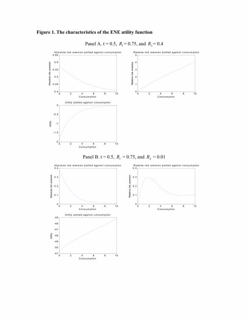
Figure 1. The characteristics of the ENE utility function

Panel A. t = 0.5, = 0.75, and = 0.4 1R 2R

0 2 4 6 8 100.4

0.45

0.5

0.55

0.6

0.65A bs o lute ris k avers ion p lo t ted agains t c ons um ption

Cons um pt ion

Abs

olut

e ris

k av

ersi

on

0 2 4 6 8 100

1

2

3

4

5R elat ive ris k avers ion p lo t ted agains t c ons um ption

Cons um pt ion

Rel

ativ

e ris

k av

ersi

on

0 2 4 6 8 10-2

-1 .5

-1

-0 .5

0Ut ility p lot ted aga ins t c ons um pt ion

Cons um pt ion

Util

ity

Panel B. t = 0.5, = 0.75, and = 0.01 1R 2R

0 2 4 6 8 100

0 .1

0 .2

0 .3

0 .4A bs o lu te ris k avers ion p lo t ted aga ins t c ons um pt ion

C ons um pt ion

Abs

olut

e ris

k av

ersi

on

0 2 4 6 8 100

0 .1

0 .2

0 .3

0 .4R ela t ive ris k avers ion p lo t ted aga ins t c ons um pt ion

C ons um pt ion

Rel

ativ

e ris

k av

ersi

on

0 2 4 6 8 10-51

-50

-49

-48

-47

-46

-45U t ilit y p lo t ted aga ins t c ons um pt ion

C ons um pt ion

Util

ity

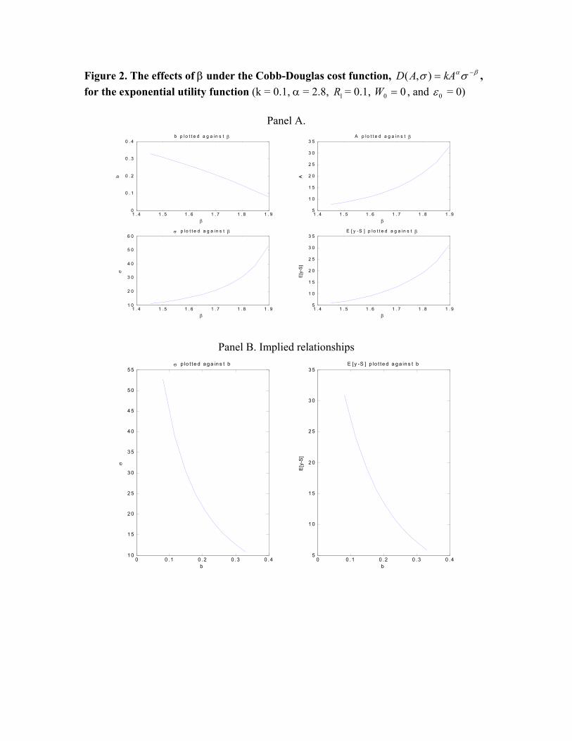
Figure 2. The effects of β under the Cobb-Douglas cost function, , for the exponential utility function (k = 0.1, α = 2.8, = 0.1,

βασσ −= kAAD ),(01R 0 =W , and 0ε = 0)

Panel A.

1 . 4 1 . 5 1 . 6 1 . 7 1 . 8 1 . 90

0 . 1

0 . 2

0 . 3

0 . 4b p lo t t e d a g a in s t β

b

β1 . 4 1 . 5 1 . 6 1 . 7 1 . 8 1 . 95

1 0

1 5

2 0

2 5

3 0

3 5A p lo t t e d a g a in s t β

A

β

1 . 4 1 . 5 1 . 6 1 . 7 1 . 8 1 . 91 0

2 0

3 0

4 0

5 0

6 0σ p lo t t e d a g a in s t β

σ

β1 . 4 1 . 5 1 . 6 1 . 7 1 . 8 1 . 95

1 0

1 5

2 0

2 5

3 0

3 5

β

E[y

-S]

E [ y -S ] p lo t t e d a g a in s t β

Panel B. Implied relationships

0 0 .1 0 .2 0 .3 0 .41 0

1 5

2 0

2 5

3 0

3 5

4 0

4 5

5 0

5 5σ p lo t te d a g a in s t b

b

σ

0 0 .1 0 .2 0 .3 0 .45

1 0

1 5

2 0

2 5

3 0

3 5

b

E[y

-S]

E [ y -S ] p lo t te d a g a in s t b

Figure 3. The effects of α under the Cobb-Douglas cost function, , for the exponential utility function (k = 0.1, β = 1.4, = 0.1,

βασσ −= kAAD ),(01R 0 =W , and 0ε = 0)

Panel A.

2 . 5 3 3 . 5 40 . 2 6

0 . 2 8

0 . 3

0 . 3 2

0 . 3 4

0 . 3 6b p lo t t e d a g a in s t α

α

b

2 . 5 3 3 . 5 42

3

4

5

6

7A p lo t t e d a g a in s t α

α

A2 . 5 3 3 . 5 45

6

7

8

9

1 0σ p lo t t e d a g a in s t α

α

σ

2 . 5 3 3 . 5 41

2

3

4

5

6

α

E[y

-S]

E [ y -S ] p lo t t e d a g a in s t α

Panel B. Implied relationships

0 . 2 6 0 . 2 8 0 . 3 0 . 3 2 0 . 3 4 0 . 3 65

5 . 5

6

6 . 5

7

7 . 5

8

8 . 5

9

9 . 5

1 0σ p lo t t e d a g a in s t b

b

σ

0 . 2 6 0 . 2 8 0 . 3 0 . 3 2 0 . 3 4 0 . 3 61 . 5

2

2 . 5

3

3 . 5

4

4 . 5

5

5 . 5

b

E[y

-S]

E [ y -S ] p lo t t e d a g a in s t b

Figure 4. The effects of initial wealth W under cost function, , for the ENE utility function (

025.0)( kAAD =

0ε = 0, t = 0.5, = 0.75, = 0.1, k = 0.1, and 1R 2R 12=σ )

Panel A.

0 0 . 0 5 0 . 1 0 . 1 5 0 . 2

0 . 1 2 8

0 . 1 3

0 . 1 3 2

b p lo t t e d a g a in s t W 0

W 0

b

0 0 . 0 5 0 . 1 0 . 1 5 0 . 2

1 . 2 8

1 . 3

1 . 3 2

A p lo t t e d a g a in s t W 0

W 0

A0 0 . 0 5 0 . 1 0 . 1 5 0 . 2

0 . 4 4 8

0 . 4 5

0 . 4 5 2

a p lo t t e d a g a in s t W 0

W 0

a

0 0 . 0 5 0 . 1 0 . 1 5 0 . 20 . 6 6

0 . 6 7

0 . 6 8

0 . 6 9

0 . 7

W 0

E[y

-S]

E [ y -S ] p lo t t e d a g a in s t W 0

Panel B. Implied relationship

0 . 1 2 7 5 0 . 1 2 8 0 . 1 2 8 5 0 . 1 2 9 0 . 1 2 9 5 0 . 1 3 0 . 1 3 0 5 0 . 1 3 1 0 . 1 3 1 5 0 . 1 3 20 . 6 6 5

0 . 6 7

0 . 6 7 5

0 . 6 8

0 . 6 8 5

0 . 6 9

0 . 6 9 5

0 . 7

b

E[y

-S]

E [ y -S ] p lo t t e d a g a in s t b

Figure 5. The effects of reservation wage 0ε under cost function, , for the ENE utility function (t = 0.5, = 0.75, = 0.1, W = 0, k = 0.1, and

25.0)( kAAD =

1R 2R 0

12=σ )

Panel A.

0 0 . 2 0 . 4 0 . 6 0 . 80 . 1 2 5

0 . 1 3

0 . 1 3 5

0 . 1 4

0 . 1 4 5b p lo t t e d a g a in s t ε 0

ε 0

b

0 0 . 2 0 . 4 0 . 6 0 . 81 . 2 5

1 . 3

1 . 3 5

1 . 4

1 . 4 5A p lo t t e d a g a in s t ε 0

ε 0

A

0 0 . 2 0 . 4 0 . 6 0 . 80 . 4

0 . 6

0 . 8

1

1 . 2

1 . 4 a p lo t t e d a g a in s t ε 0

ε 0

a

0 0 . 2 0 . 4 0 . 6 0 . 80

0 . 2

0 . 4

0 . 6

0 . 8

ε 0

E[y

-S]

E [ y -S ] p lo t t e d a g a in s t ε 0

Panel B. Implied relationship

0 .1 2 8 0 .1 3 0 .1 3 2 0 .1 3 4 0 .1 3 6 0 .1 3 8 0 .1 4 0 .1 4 2 0 .1 4 40

0 .1

0 .2

0 .3

0 .4

0 .5

0 .6

0 .7

b

E[y

-S]

E [ y -S ] p lo t t e d a g a in s t b

Figure 6. The effects of initial wealth W under the Cobb-Douglas cost function, , for the ENE utility function (t = 0.5, = 0. 75, = 0.1,

0βασσ −= kAAD ),( 1R 2R 0ε =

0, k=0.1, α = 2.8, and β = 1.4)

Panel A.

0 0 .0 5 0 .1 0 .1 5 0 .2-0 .4

-0 .2

0

0 .2

0 .4

W 0

a

a p lo t te d a g a in s t W 0

0 0 .0 5 0 .1 0 .1 5 0 .20 .3

0 .3 0 5

0 .3 1

0 .3 1 5

0 .3 2

0 .3 2 5

0 .3 3

W 0

b

b p lo t te d a g a in s t W 0

0 0 .0 5 0 .1 0 .1 5 0 .22 .5

2 .6

2 .7

2 .8

2 .9

W 0

A

A p lo t t e d a g a in s t W 0

0 0 .0 5 0 .1 0 .1 5 0 .22 .8

3

3 .2

3 .4

3 .6

3 .8

W 0

σ

σ p lo t t e d a g a in s t W 0

Panel B. Implied relationships

0 0.05 0.1 0.15 0.21.4

1.6

1.8

2

2.2

W 0

E[y

-S]

E [y -S ] plot ted agains t W 0

0.3 0.31 0.32 0.332.8

3

3.2

3.4

3.6

3.8

b

σ

σ plot ted agains t b

0.3 0.31 0.32 0.331.4

1.6

1.8

2

2.2

b

E[y

-S]

E [y -S ] plot ted agains t b

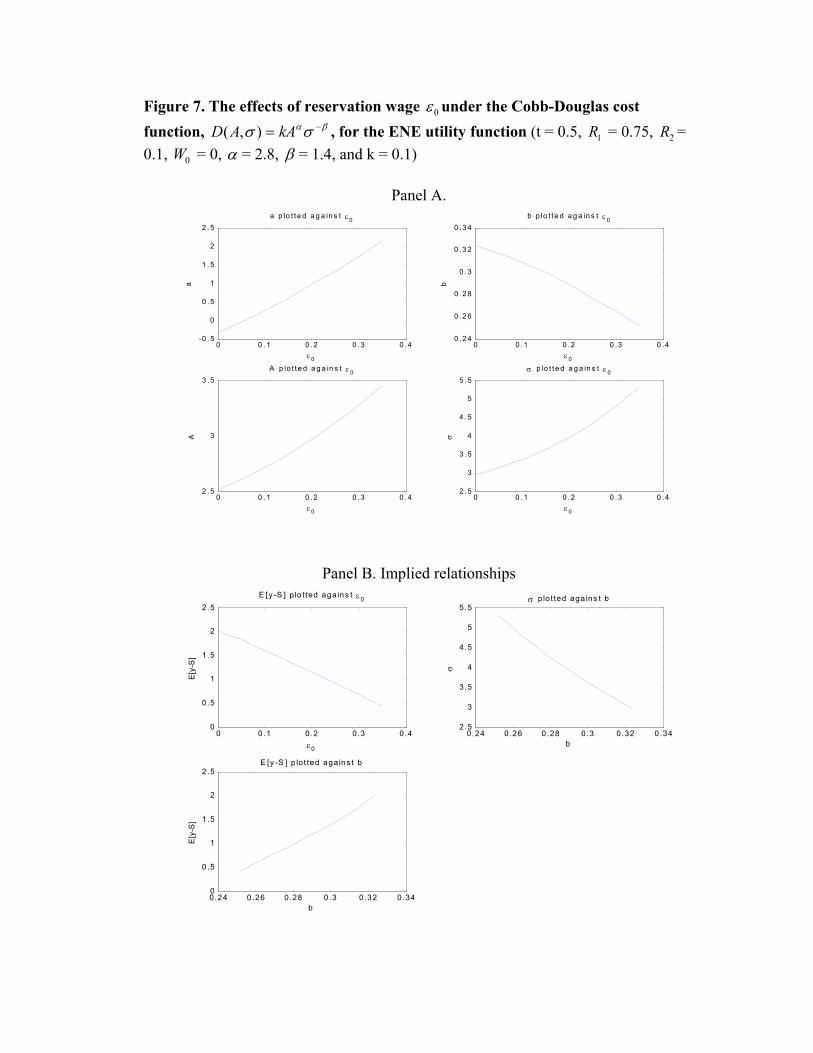
Figure 7. The effects of reservation wage 0ε under the Cobb-Douglas cost function, , for the ENE utility function (t = 0.5, = 0.75, = 0.1, W = 0,

βασσ −= kAAD ),( 1R 2R

0 α = 2.8, β = 1.4, and k = 0.1)

Panel A.

0 0 .1 0 .2 0 .3 0 .4-0 .5

0

0 .5

1

1 .5

2

2 .5a p lo t t e d a g a in s t ε 0

ε 0

a

0 0 .1 0 .2 0 .3 0 .40 .2 4

0 .2 6

0 .2 8

0 .3

0 .3 2

0 .3 4b p lo t t e d a g a in s t ε 0

ε 0

b

0 0 .1 0 .2 0 .3 0 .42 .5

3

3 .5A p lo t te d a g a in s t ε 0

ε 0

A

0 0 .1 0 .2 0 .3 0 .42 .5

3

3 .5

4

4 .5

5

5 .5σ p lo t te d a g a in s t ε 0

ε 0

σ

Panel B. Implied relationships

0 0.1 0.2 0.3 0.40

0.5

1

1.5

2

2.5

ε0

E[y

-S]

E [y -S ] p lo t ted agains t ε0

0 .24 0.26 0.28 0.3 0.32 0.342.5

3

3.5

4

4.5

5

5.5σ p lo t ted aga ins t b

b

σ

0.24 0.26 0.28 0.3 0.32 0.340

0.5

1

1.5

2

2.5

b

E[y

-S]

E [y -S ] p lot ted aga ins t b

Figure 8. The effects of under the Cobb-Douglas cost function, , for the ENE utility function (k = 0.1, t = 0.5, = 0.75, W = 0,

2Rβασσ −= kAAD ),(

0

1R 0

ε = 0, α = 2.8, and β = 1.4)

Panel A.

0 0 .1 0 .2 0 .3 0 .4 0 .5-0 .33

-0 .32

-0 .31

-0 .3

-0 .29

-0 .28

R 2

a

a p lo t te d a ga in s t R 2

0 0 .1 0 .2 0 .3 0 .4 0 .50 .31

0 .32

0 .33

0 .34

0 .35

R 2

b

b p lo t te d a ga in s t R 2

0 0 .1 0 .2 0 .3 0 .4 0 .52

2 .2

2 .4

2 .6

2 .8

R 2

A

A p lo t ted a g a in s t R 2

0 0 .1 0 .2 0 .3 0 .4 0 .52 .2

2 .4

2 .6

2 .8

3

3 .2

R 2

σ

σ p lo t ted a g a in s t R 2

Panel B. Implied relationships

0 0.1 0.2 0.3 0.4 0.51.6

1.8

2

2.2

2.4

R 2

E[y

-S]

E [y -S ] p lo t ted agains t R 2

0.31 0.32 0.33 0.34 0.352.2

2.4

2.6

2.8

3

3.2σ p lo t ted aga ins t b

b

σ

0.31 0.32 0.33 0.34 0.351.6

1.8

2

2.2

2.4

b

E[y

-S]

E [y -S ] p lot ted aga ins t b

Figure 9-1. The effects of α under the Cobb-Douglas cost function,

, for the ENE utility function (k = 0.1, t = 0.5, = 0.75, = 0.1, W = 0,

βασσ −= kAAD ),(

0 0

1R 2Rε = 0, and β = 1.4)

Panel A.

2 .8 3 3 . 2 3 . 4 3 .6 3 .8-0 . 3 2

-0 .3

-0 . 2 8

-0 . 2 6

-0 . 2 4

-0 . 2 2

-0 .2

α

a

a p lo t t e d a g a in s t α

2 .8 3 3 . 2 3 . 4 3 .6 3 .80 . 2 8

0 . 2 9

0 .3

0 . 3 1

0 . 3 2

0 . 3 3

α

b

b p lo t t e d a g a in s t α

2 .8 3 3 . 2 3 . 4 3 .6 3 .81

1 .5

2

2 .5A p lo t t e d a g a in s t α

α

A

2 . 8 3 3 . 2 3 . 4 3 .6 3 .82

2 .2

2 .4

2 .6

2 .8

3σ p lo t t e d a g a in s t α

α

σ

Panel B. Implied relationships

2 .8 3 3 .2 3 .4 3 .6 3 .81

1 .2

1 .4

1 .6

1 .8

2

α

E[y

-S]

E [ y -S ] p lo t t e d a g a in s t α

0 .2 8 0 .2 9 0 .3 0 .3 1 0 .3 2 0 .3 32

2 .2

2 .4

2 .6

2 .8

3σ p lo t t e d a g a in s t b

b

σ

0 .2 8 0 .2 9 0 .3 0 .3 1 0 .3 2 0 .3 31

1 .2

1 .4

1 .6

1 .8

2

b

E[y

-S]

E [ y -S ] p lo t t e d a g a in s t b

Figure 9-2. The effects of β under the Cobb-Douglas cost function, , for the ENE utility function (k = 0.1, t = 0.5, = 0.75, =

0.1, W = 0,

βασσ −= kAAD ),(

0 0

1R 2Rε = 0, and α = 2.8)

Panel A.

1 .6 5 1 .7 1 .7 5 1 .8 1 .8 5-0 .2 4

-0 .2 2

-0 .2

-0 .1 8

-0 .1 6

-0 .1 4

β

a

a p lo t t e d a g a in s t β

1 .6 5 1 .7 1 .7 5 1 .8 1 .8 50 .1

0 .1 2

0 .1 4

0 .1 6

0 .1 8

0 .2

β

b

b p lo t t e d a g a in s t β

1 .6 5 1 .7 1 .7 5 1 .8 1 .8 53

3 .5

4

4 .5

5A p lo t te d a g a in s t β

β

A

1 .6 5 1 .7 1 .7 5 1 .8 1 .8 54

5

6

7

8σ p lo t te d a g a in s t β

β

σ

Panel B. Implied relationships

1.65 1.7 1.75 1.8 1.853

3.5

4

4.5

β

E[y

-S]

E [y -S ] plot ted agains t β

0.1 0.12 0.14 0.16 0.18 0.24

5

6

7

8σ plot ted agains t b

b

σ

0.1 0.12 0.14 0.16 0.18 0.23

3.5

4

4.5

b

E[y

-S]

E [y -S ] plotted agains t b

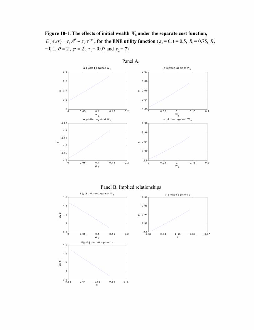
Figure 10-1. The effects of initial wealth W under the separate cost function, , for the ENE utility function (

0ψθ σττσ −+= 21),( AAD 0ε = 0, t = 0.5, = 0.75,

= 0.1, 1R 2R

2=θ , 2=ψ , 1τ = 0.07 and 2τ = 7)

Panel A.

0 0.05 0.1 0.15 0.20

0.2

0.4

0.6

0.8

W 0

a

a p lot ted aga ins t W 0

0 0.05 0.1 0.15 0.20.63

0.64

0.65

0.66

0.67

W 0

b

b p lot ted aga ins t W 0

0 0.05 0.1 0.15 0.24.5

4.55

4.6

4.65

4.7

4.75

W 0

A

A p lo t ted agains t W 0

0 0.05 0.1 0.15 0.22.9

2.92

2.94

2.96

2.98

W 0

σ

σ p lo t ted agains t W 0

Panel B. Implied relationships

0 0 .0 5 0 .1 0 .1 5 0 .20 .8

1

1 .2

1 .4

1 .6

W 0

E[y

-S]

E [ y -S ] p lo t te d a g a in s t W 0

0 .6 3 0 .6 4 0 .6 5 0 .6 6 0 .6 72 .9

2 .9 2

2 .9 4

2 .9 6

2 .9 8

b

σ

σ p lo t te d a g a in s t b

0 .6 3 0 .6 4 0 .6 5 0 .6 6 0 .6 70 .8

1

1 .2

1 .4

1 .6

b

E[y

-S]

E [ y -S ] p lo t te d a g a in s t b

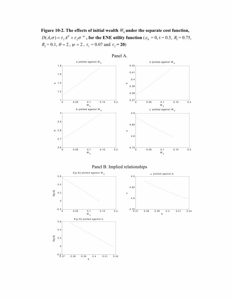
Figure 10-2. The effects of initial wealth W under the separate cost function, , for the ENE utility function (

0ψθ σττσ −+= 21),( AAD 0ε = 0, t = 0.5, = 0.75,

= 0.1, 1R

2R 2=θ , 2=ψ , 1τ = 0.07 and 2τ = 20)

Panel A.

0 0.05 0.1 0.15 0.21

1.2

1.4

1.6

1.8

W 0

a

a p lot ted agains t W 0

0 0.05 0.1 0.15 0.20.37

0.38

0.39

0.4

0.41

0.42

W 0

b

b p lot ted agains t W 0

0 0.05 0.1 0.15 0.22.6

2.7

2.8

2.9

3

W 0

A

A p lotted agains t W 0

0 0.05 0.1 0.15 0.24.75

4.8

4.85

4.9

W 0

σ

σ p lotted agains t W 0

Panel B. Implied relationships

0 0 .0 5 0 .1 0 .15 0 .2-0 .2

0

0 .2

0 .4

0 .6

W 0

E[y

-S]

E [y -S ] p lo t te d ag a ins t W 0

0 .37 0 .3 8 0 .39 0 .4 0 .4 1 0 .4 24 .75

4 .8

4 .85

4 .9

b

σ

σ p lo t ted a g a in s t b

0 .37 0 .3 8 0 .39 0 .4 0 .4 1 0 .4 2-0 .2

0

0 .2

0 .4

0 .6

b

E[y

-S]

E [y -S ] p lo t te d ag a ins t b