Incentives and creativity: evidence from the academic life

RAND Journal of EconomicsVol. 42, No. 3, Fall 2011pp. 527–554

Incentives and creativity: evidence fromthe academic life sciences

Pierre Azoulay∗Joshua S. Graff Zivin∗∗and

Gustavo Manso∗∗∗

Despite its presumed role as an engine of economic growth, we know surprisingly little aboutthe drivers of scientific creativity. We exploit key differences across funding streams withinthe academic life sciences to estimate the impact of incentives on the rate and direction ofscientific exploration. Specifically, we study the careers of investigators of the Howard HughesMedical Institute (HHMI), which tolerates early failure, rewards long-term success, and givesits appointees great freedom to experiment, and grantees from the National Institutes of Health(NIH), who are subject to short review cycles, predefined deliverables, and renewal policiesunforgiving of failure. Using a combination of propensity-score weighting and difference-in-differences estimation strategies, we find that HHMI investigators produce high-impact articlesat a much higher rate than a control group of similarly accomplished NIH-funded scientists.Moreover, the direction of their research changes in ways that suggest the program induces themto explore novel lines of inquiry.

1. Introduction

� In 1980, a scientist from the University of Utah, Mario Capecchi, applied for a grant atthe National Institutes of Health (NIH). The application contained three projects. The NIH peerreviewers liked the first two projects, which were building on Capecchi’s past research efforts, butthey were unanimously negative in their appraisal of the third project, in which he proposed todevelop gene targeting in mammalian cells. They deemed the probability that the newly introducedDNA would ever find its matching sequence within the host genome vanishingly small and theexperiments not worthy of pursuit. The NIH funded the grant despite this misgiving, but strongly

∗Massachusetts Institute of Technology and NBER; [email protected].∗∗University of California, San Diego and NBER; [email protected].∗∗∗Massachusetts Institute of Technology; [email protected] gratefully acknowledge the financial support of the Kauffman Foundation and the National Science Foundationthrough its SciSIP Program (award no. SBE-0738142). We thank Peter Cebon, Thomas Cech, Purnell Choppin, DavidClayton, Nico Lacetera, Antoinette Schoar, Scott Stern, Jerry Thursby, Heidi Williams, and two anonymous referees foruseful comments and suggestions. The usual disclaimer applies.

Copyright C© 2011, RAND. 527

528 / THE RAND JOURNAL OF ECONOMICS

recommended that Capecchi drop the third project. In his retelling of the story, the scientistwrites that despite this unambiguous advice, he chose to put almost all his efforts into the thirdproject: “It was a big gamble. Had I failed to obtain strong supporting data within the designatedtime frame, our NIH funding would have come to an abrupt end and we would not be talkingabout gene targeting today” (Capecchi, 2008). Fortunately, within four years, Capecchi and histeam obtained strong evidence for the feasibility of gene targeting in mammalian cells, and in1984 the grant was renewed enthusiastically. Dispelling any doubt that he had misinterpretedthe feedback from reviewers in 1980, the critique for the 1984 competitive renewal started, “Weare glad that you didn’t follow our advice.” The story does not stop there. In September 2007,Capecchi shared the Nobel Prize for developing the techniques to make knockout mice with OliverSmithies and Martin Evans. Such mice have allowed scientists to learn the roles of thousands ofmammalian genes and provided laboratory models of human afflictions in which to test potentialtherapies.

Across all of the social sciences, researchers often model the creative process as thecumulative, interactive recombination of existing bits of knowledge in novel ways (Weitzman,1998; Burt, 2004; Simonton, 2004). But the combinatoric metaphor does not speak directlyto the important tradeoff illustrated by the anecdote above. Some discoveries are incrementalin nature, and reflect the fine-tuning of previously available technologies or the exploitationof established scientific trajectories. Others are more radical and require the exploration of new,untested approaches. Both forms of innovation are valuable, but we still have a poor understandingof what drives radical innovation. One view is that radical innovation happens by accident. FromArchimedes’ eureka moment to Newton’s otherworldly contemplation interrupted by the fallof an apple, luck (and sometimes talent) play an essential role in lay theories of breakthroughinnovation. Of course, if luck and talent exhaust the list of ingredients necessary to producebreakthroughs, then there is little for economists to contribute.

In the anecdote reported above, the scientist was undeterred by his peers’ advice to “playit safe,” and eventually saw his bold ideas prevail. If incentives play an important role in theproduction of novel ideas, this heroic story might be atypical. In this article, we provide empiricalevidence that nuanced features of incentive schemes embodied in the design of research contractsexert a profound influence on the subsequent development of breakthrough ideas. The challengeis to find a setting in which (i) radical innovation is a key concern; (ii) agents are at risk ofreceiving different incentive schemes; and (iii) it is possible to measure innovative output and todistinguish between incremental and radical ideas. We argue that the academic life sciences inthe United States provides an excellent testing ground.

Specifically, we study the careers of researchers who can be funded through two very distinctmechanisms: investigator-initiated R01 grants from the NIH, or support from the Howard HughesMedical Institute (HHMI) through its investigator program. HHMI, a non-profit medical researchorganization, plays a powerful role in advancing biomedical research and science education inthe United States. The institute commits almost $700 million a year—a larger amount than theNational Science Foundation biological sciences program, for example. HHMI’s stated goal is to“push the boundaries of knowledge” in some of the most important areas of biological research.To do so, the HHMI program has adopted practices that according to Manso (2011) shouldprovide strong incentives for breakthrough scientific discoveries: the award cycles are long (fiveyears, and typically renewed at least once); the review process provides detailed, high-qualityfeedback to the researcher; and the program selects “people, not projects,” which allows (and infact encourages) the quick reallocation of resources to new approaches when the initial ones arenot fruitful.1 This stands in sharp contrast with the incentives faced by life scientists funded bythe NIH. The typical R01 grant cycle lasts only three years, and renewal is not very forgivingof failure. Feedback on performance is limited in its depth. Importantly, the NIH funds projects

1 Though not part of Manso’s (2011) initial analysis, we extend his model in Appendix A to show that providingthe researcher greater latitude in her search activities encourages exploration.

C© RAND 2011.

AZOULAY, GRAFF ZIVIN, AND MANSO / 529

with clearly defined deliverables, not individual scientists, which could increase the costs ofexperimentation.

The contrast between the HHMI and NIH grant mechanisms naturally leads to the questionof whether HHMI-style incentives result in a higher rate of production of particularly valuableideas. Three significant hurdles must be overcome to answer this question.

First, we need to identify a group of NIH-funded scientists who are appropriate controlsfor the researchers selected into the HHMI program. Given the high degree of accomplishmentexhibited by HHMI investigators at the time of their appointment, a random sample of scientistsof the same age, working in the same fields, would not be appropriate. In the absence of aplausible source of exogenous variation for HHMI appointment, we estimate the treatment effectof the program by contrasting HHMI-funded scientists’ output with that of a group of NIH-fundedscientists who focus their research on the same subfields of the life sciences as HHMI investigatorsand received prestigious early career prizes. Furthermore, using an in-depth understanding ofthe HHMI appointment process, we cull from this control group scientists who look similarto the HHMI investigators on the observable factors that we know to be relevant for selection intothe HHMI program.

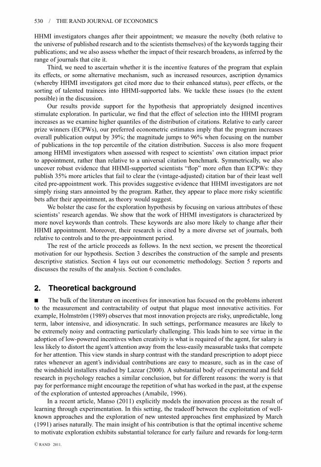
Second, we must be able to distinguish particularly creative contributions from incrementaladvances. Although we investigate the effect of the program on the raw number of originalresearch articles published, the bulk of our analysis focuses on the number of publications thatfall into different quantiles of the vintage-specific, article-level distribution of citations (seeFigure 1): top quartile, top five percentiles, and top percentile. We also use these scientists’own citation impact in the pre-appointment period to ask whether they often outperform theirmost heavily cited article, and conversely, whether they often publish articles that garner lesscitations than their least-cited article. Another prong in our attempt to measure creativity is tomeasure explorative behavior directly. Specifically, we examine whether the research agenda of

FIGURE 1

MEASURING THE TAIL OF THE DISTRIBUTION OF CITATIONS

0

50

100

150

200

250

Num

ber

of c

itatio

ns

1970 1975 1980 1985 1990 1995 2000 2005

Selected quantilesarticle-level distribution of citations

Top 1%

Top 5%

Top 25%

Top 50%

Selected quantiles (0.50, 0.25, 0.05, and 0.01) for the vintage-specific empirical distribution of the number of citationsat the article level. These quantiles were computed in early 2008 using the universe of all articles indexed by ISI/Web ofScience that appeared in life science journals.

C© RAND 2011.


HHMI investigators changes after their appointment; we measure the novelty (both relative tothe universe of published research and to the scientists themselves) of the keywords tagging theirpublications; and we also assess whether the impact of their research broadens, as inferred by therange of journals that cite it.

Third, we need to ascertain whether it is the incentive features of the program that explainits effects, or some alternative mechanism, such as increased resources, ascription dynamics(whereby HHMI investigators get cited more due to their enhanced status), peer effects, or thesorting of talented trainees into HHMI-supported labs. We tackle these issues (to the extentpossible) in the discussion.

Our results provide support for the hypothesis that appropriately designed incentivesstimulate exploration. In particular, we find that the effect of selection into the HHMI programincreases as we examine higher quantiles of the distribution of citations. Relative to early careerprize winners (ECPWs), our preferred econometric estimates imply that the program increasesoverall publication output by 39%; the magnitude jumps to 96% when focusing on the numberof publications in the top percentile of the citation distribution. Success is also more frequentamong HHMI investigators when assessed with respect to scientists’ own citation impact priorto appointment, rather than relative to a universal citation benchmark. Symmetrically, we alsouncover robust evidence that HHMI-supported scientists “flop” more often than ECPWs: theypublish 35% more articles that fail to clear the (vintage-adjusted) citation bar of their least wellcited pre-appointment work. This provides suggestive evidence that HHMI investigators are notsimply rising stars annointed by the program. Rather, they appear to place more risky scientificbets after their appointment, as theory would suggest.

We bolster the case for the exploration hypothesis by focusing on various attributes of thesescientists’ research agendas. We show that the work of HHMI investigators is characterized bymore novel keywords than controls. These keywords are also more likely to change after theirHHMI appointment. Moreover, their research is cited by a more diverse set of journals, bothrelative to controls and to the pre-appointment period.

The rest of the article proceeds as follows. In the next section, we present the theoreticalmotivation for our hypothesis. Section 3 describes the construction of the sample and presentsdescriptive statistics. Section 4 lays out our econometric methodology. Section 5 reports anddiscusses the results of the analysis. Section 6 concludes.

2. Theoretical background

� The bulk of the literature on incentives for innovation has focused on the problems inherentto the measurement and contractability of output that plague most innovative activities. Forexample, Holmstrom (1989) observes that most innovation projects are risky, unpredictable, longterm, labor intensive, and idiosyncratic. In such settings, performance measures are likely tobe extremely noisy and contracting particularly challenging. This leads him to see virtue in theadoption of low-powered incentives when creativity is what is required of the agent, for salary isless likely to distort the agent’s attention away from the less-easily measurable tasks that competefor her attention. This view stands in sharp contrast with the standard prescription to adopt piecerates whenever an agent’s individual contributions are easy to measure, such as in the case ofthe windshield installers studied by Lazear (2000). A substantial body of experimental and fieldresearch in psychology reaches a similar conclusion, but for different reasons: the worry is thatpay for performance might encourage the repetition of what has worked in the past, at the expenseof the exploration of untested approaches (Amabile, 1996).

In a recent article, Manso (2011) explicitly models the innovation process as the result oflearning through experimentation. In this setting, the tradeoff between the exploitation of well-known approaches and the exploration of new untested approaches first emphasized by March(1991) arises naturally. The main insight of his contribution is that the optimal incentive schemeto motivate exploration exhibits substantial tolerance for early failure and rewards for long-term

C© RAND 2011.


success. Tolerance for early failure allows the agent to explore in the early stages of the contractualrelationship without incurring the usual negative consequences of lower pay or termination. Atthe same time, reward for long-term success prevents the agent from shirking early on and inducesthe agent to explore new ideas that will allow him to perform well in the longrun. The principalcan more effectively motivate exploration if he can commit not to terminate an agent after poorshort-term performance, even if it is ex post efficient for the principal to do so. Another importantingredient of Manso’s model is timely feedback on performance. Providing information to theagent about how well he is doing allows the agent to explore more efficiently, reducing the costsof experimentation. An agent who does not get feedback on performance may waste more timeon unfruitful ideas.

Empirical evidence on the effects of long-term incentives is scant. Most relevant to thefindings presented below is Lerner and Wulf’s (2007) study of corporate R&D lab heads.They show that higher levels of deferred compensation are associated with the production ofmore heavily cited patents, whereas short-term incentives bear no relationship to firm innovativeperformance. In a similar vein, Tian and Wang (2010) show that start-up firms backed by morefailure-tolerant venture capitalists are more innovative ex post. The present article presents thefirst systematic attempt to isolate, in a field setting, the effect of the bundle of incentive practicesidentified by Manso (2011) on exploration and creativity at the individual level (see Ederer andManso, 2010 for experimental evidence with a similar flavor). We believe that the academiclife sciences in the United States provide an appropriate setting, first and foremost because itprovides naturally occurring variation in incentives that closely matches the contrast betweenpay-for-performance and exploration-type schemes emphasized by Manso (2011).

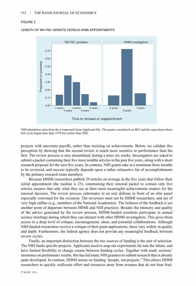
Most academic life scientists must rely on grants from the NIH, the largest public funder ofbiomedical research in the United States. With an annual budget of $28.4 billion in 2007, supportfrom the NIH dwarfs that available from other public or private funders, including the NationalScience Foundation ($6 billion in 2007) or the American Cancer Society ($147 million in 2007).The most common type of NIH grant for investigator-initiated projects is the R01 grant. In 2007,their average amount was $225,000 in annual direct costs, and the awards last for a typical three tofive years before coming up for renewal (see Figure 2). The NIH “study sections,” or peer-reviewpanels in charge of allocating awards, are notoriously risk averse and often insist on a great deal ofpreliminary evidence before deciding to fund a project. This often leads researchers to resubmittheir applications several times and to multiply the number of applications, taking time awayfrom productive research activities. It is an often-heard complaint among academic biomedicalresearchers that study sections’ prickliness encourages them to pursue relatively safe avenuesthat build directly on previous results, at the expense of truly exploratory research (Kaplan, 2005;Kolata, 2009; McKnight, 2009).

An alternative funding mechanism is provided by the investigator program of the HHMI.This program “urges its researchers to take risks, to explore unproven avenues, to embrace theunknown—even if it means uncertainty or the chance of failure.”2 New appointments are basedon nominations from research institutions; once selected, researchers continue to be based at theirinstitutions, typically leading a research group of 10–25 students, postdoctoral associates, andtechnicians. In its stated policies, HHMI departs in striking fashion from NIH’s funding practices,in ways that should bring incentives in line with the type of schemes suggested by Manso (2011).HHMI investigators are initially appointed for five years,3 and in the case of termination, there isa two-year phase-down period during which the researcher continues to be funded, allowing herto search for other sources of funding without having to close down her lab.

Moreover, HHMI investigators appear to share the perception that their first appointmentreview is rather lax, with reviewers more interested in making sure that they have taken on new

2 See www.hhmi.org/research/investigators/3 Appointment lengths have varied over the history of the program; more detailed information will be provided in

the data section.

C© RAND 2011.


FIGURE 2

LENGTH OF NIH R01 GRANTS VERSUS HHMI APPOINTMENTS

0.00

0.10

0.20

0.30

0.40

0.50

0.60

0.70

2 years3 years

4 years5 years

6 years 3 years5 years

7 years

NIH R01 grantees HHMI investigatorsP

ropo

rtio

n of

sci

entis

ts

Time to renewal or reappointment

NIH tabulations stem from the Compound Grant Applicant File. The grants considered are R01 and the equivalent whosefirst cycle began later than 1970 but earlier than 2002.

projects with uncertain payoffs, rather than insisting on achievements. Below, we validate thisperception by showing that the second review is much more sensitive to performance than thefirst. The review process is also streamlined, lasting a mere six weeks. Investigators are asked tosubmit a packet containing their five most notable articles in the past five years, along with a shortresearch proposal for the next five years. In contrast, NIH grants take at a minimum three monthsto be reviewed, and success typically depends upon a rather exhaustive list of accomplishmentsby the primary research team members.

Because HHMI researchers publish 29 articles on average in the five years that follow theirinitial appointment (the median is 25), constraining their renewal packet to contain only fivearticles ensures that only what they see as their most meaningful achievements matters for therenewal decision. The review process culminates in an oral defense in front of an elite panelespecially convened for the occasion. The reviewers must not be HHMI researchers, and are ofvery high caliber (e.g., members of the National Academies). The richness of the feedback is yetanother point of departure between HHMI and NIH practices. Besides the intensity and qualityof the advice generated by the review process, HHMI-funded scientists participate in annualscience meetings during which they can interact with other HHMI investigators. This gives themaccess to a deep level of critique, encouragement, ideas, and potential collaborations. AlthoughNIH-funded researchers receive a critique of their grant applications, these vary widely in qualityand depth. Furthermore, the federal agency does not provide any meaningful feedback betweenreview cycles.

Finally, an important distinction between the two sources of funding is the unit of selection.The NIH funds specific projects. Applicants need to map out experiments far into the future, andhave limited flexibility to change course between funding cycles. Together with study sections’insistence on preliminary results, this has led many NIH grantees to submit research that is alreadyquite developed. In contrast, HHMI insists on funding “people, not projects.” This allows HHMIresearchers to quickly reallocate effort and resources away from avenues that do not bear fruit.

C© RAND 2011.


TABLE 1 Comparison between the Two Sources of Funding

NIH R01 Grants HHMI Investigator Program

Three- to five-year funding Five-year fundingFirst review is similar to any other review First review is rather laxFunds dry up upon nonrenewal Two-year phase-down upon nonrenewalSome feedback in the renewal process Feedback from renowned scientistsFunding is for a particular project “People, not projects”

The economics literature (e.g., Aghion, Dewatripont, and Stein, 2008) views unfettered controlover one’s research agenda as the key distinguishing feature of innovative activities performedin academia (relative to the private sector). Variation in the unit of selection reminds us thatthe degree of effective control experienced by academic researchers often depends on the arcanedetails of funding mechanisms. Although not part of Manso’s (2011) initial analysis, we extendhis model in Appendix A to show that providing the researcher greater latitude in her searchactivities encourages exploration. Table 1 summarizes the main differences between the twosources of funding.

3. Data and sample characteristics

� This section provides a detailed description of the process through which the data used inthe econometric analysis were assembled. In order, we describe (i) the Howard Hughes Medicalinvestigator sample; (ii) the set of control investigators against which the HHMI scientists willbe compared; and (iii) our metrics of scientific creativity. We also present relevant descriptivestatistics.

� HHMI sample. We begin with a basic description of the criteria necessary for nominationand appointment as an HHMI investigator. To be eligible, a scientist must be tenured or on thetenure track at a major research university, academic medical center, or research institute. Thesubfields of the life sciences of interest to HHMI investigators are quite broad, but have tended toconcentrate on cell and molecular biology, neurobiology, immunology, and biochemistry. Career-stage considerations have varied over time, although HHMI typically has not appointed scientistsuntil they have had enough independent experience so that their work can be distinguished fromthat of their postdoctoral or graduate school adviser.

Upon receipt of nominations from participating institutions, HHMI empanels a jury thatreviews these nominations in two sequential steps. In a first step, the number of nominees iswhittled down to a manageable number, mostly based on observable characteristics. For example,NIH-funded investigators have an advantage because the panel of judges interprets receipt offederal grants as a signal of management ability. The jury also looks for evidence that thenominee has stepped out of the shadow cast by his/her mentors: an independent research agenda,and a “big hit,” that is, a high-impact publication in which the mentor’s name does not appearon the coauthorship list. In a second step, each remaining nominee’s credentials and future plansare given an in-depth qualitative look.4 Finally, until recently, appointment contracts varied intheir initial length. Assistant investigators (assistant professors in their home institution) wereappointed for three years; associate investigators, for five years; and investigators, for seven years.5

4 Although an input into this process is a letter grade, the review does not provide a continuous score that couldbe used in a regression discontinuity-type framework. Moreover, the cutoff that separates successful from unsuccessfulnominees is endogenous in the sense that it depends on the overall quality of the applicant pool.

5 In our sample, these categories respectively account for 15%, 70%, and 15% of the total number of scientists inthe treatment group. Of course, such variation raises the specter that appointment length might be endogenous. In fact,the length of the initial term is purely a function of the scientist’s academic rank in his/her home institution.

C© RAND 2011.


Our analysis focuses on HHMI investigators appointed in 1993, 1994, and 1995. We excludethe three researchers that withdrew from the program voluntarily, leaving us with a sample of 73scientists.6

� Control sample: early career prize winners. In the absence of information on the runners-up of the HHMI competitions, we must rely on observable characteristics to create viable controlgroups. The main challenge is that HHMI investigators are extremely accomplished at the time oftheir appointment. Controls should not only be well matched with HHMI investigators in termsof fields, age, gender, and host institutions; their accomplishments should also be comparable atbaseline. Our control group is drawn from early career prize winners in the life sciences.

The Pew, Searle, Beckman, Packard, and Rita Allen scholarships are early career prizes thattarget scientists in the same life science subfields and similar research institutions as HHMI.Every year, these charitable trusts provide seed funding to around 60 life scientists in the first twoyears of their independent careers. These scholarships are among the most prestigious accoladesthat young researchers can receive as they are building a laboratory, but they differ from HHMIinvestigatorships in one essential respect: they are structured as one-time grants (e.g., $60,000a year over four years for the Pew Scholarship; $80,000 a year for three years for the SearleScholarship, etc.). These amounts are relatively small, roughly corresponding to 35% of a typicalNIH R01 grant. As a result, these scholars must still attract grants from other funding sources(especially NIH) if they intend to further their independent research career. After a screen toeliminate investigators whose age places them outside the age range of the treatment group,and a second screen to exclude researchers working in idiosyncratic fields, we are left with 393scientists awarded one of these scholarships.

Before presenting descriptive statistics, it is useful to discuss broad features of the controlgroup that will influence the interpretation of the treatment effect. The process that results in theselection of HHMIs and controls is very similar. In both cases, an elite jury of senior scientists isgiven the mission to identify individuals with an impressive track record as well as exceptionalpromise; in particular, they are not asked to evaluate the merits of an individual project. The maindifference between these programs is that ECPWs are selected at the very start of their independentcareer, when it is difficult to distinguish their output from that of their postdoctoral mentor. Incontrast, the modal HHMI investigator stands at the cusp of the tenure decision when s/he is ap-pointed. As a result, there is more variability in the expected performance of ECPW scholars thanis the case among HHMI investigators but, as we will show, it is possible to cull from this groupa subsample of scientists whose characteristics match well those of HHMI scientists at baseline.

� Measuring scientific creativity. Creativity is a loaded term. The Wikipedia entry informsus that more than 60 different definitions can be found in the psychological literature, none ofwhich is particularly authoritative. Furthermore, there exists no agreed-upon metrics or techniquesto measure creative outputs.

The perspective adopted in this article is very pragmatic, and guided by the constraints puton us by the availability of data. Amabile (1996) suggests that whereas innovation “begins withcreative ideas...creativity by individuals and teams is a starting point for innovation; the first is anecessary but not sufficient condition for the second.” Although we certainly agree with this viewat a conceptual level, the measurement of scientific productivity—an already well-establisheddiscipline—makes it hard to recognize this nuance. A crucial development in the bibliometricliterature has been the use of citation information to adjust raw publication counts for quality.Such an approach is not entirely satisfying here, as both “humdrum” and “breakthrough” research

6 One accepted a top administrative position in his/her university (HHMI rules prevent investigators from holdingmajor administrative posts), and one moved to an institution that had no relationship with HHMI. Yet another wishedto move to a different institution during his/her first appointment. To prevent the eruption of bidding wars over HHMIinvestigators, the institute forces such investigators to resign their appointment.

C© RAND 2011.


generate publications and citations. Moreover, some types of publications, like review articles,tend to generate a number of citations not commensurate with their degree of originality. Ithas long been noted that the distributions of publications and citations at the individual level isextremely skewed, and typically follows a power law (Lotka, 1926). The distribution of citationsat the article level exhibits even more skewness. In this article, we make use of the wide variationin impact across the publications of a given scientist to compute measures of creative output.Specifically, we sum the number of distinct contributions that fall into the higher quantiles (topquartile, top five percentiles, or top percentile) of the article-level distribution of citations for anindividual scientist in a given time period.

One practical hurdle is truncation: older articles have had more time to be cited, and henceare more likely to reach the tail of the citation distribution. To overcome this issue, we compute adifferent empirical cumulative distribution function in each year.7 For example, in the life sciencesbroadly defined, an article published in 1980 would require at least 98 citations to fall into the topfive percentiles of the distribution; an article published in 1990, 94 citations; and an article pub-lished in 2000, only 57 citations (this is illustrated in Figure 1). With these empirical distributionsin hand, it becomes meaningful to count the number of articles that fall, for example, in the toppercentile over a scientist’s career. Counting the number of contributions that fall “in the tail” ispredicated on the idea that exploration is more likely to result in high-impact publications, relativeto exploitation.8 We also assess impact relative to each scientist’s own pre-appointment citationperformance. Because there are not enough data to estimate individual, vintage-specific citationdistributions, we use the entire corpus of work published up until the year of appointment (1993,1994, or 1995) to compute the citation quantile corresponding to each scientist’s most heavilycited article. We then count the number of times a scientist exceeds this level after appointment.

We rely on two additional metrics of scientific excellence. We tabulate elections to theNational Academy of Sciences. We also measure the number of students and fellows trained in ascientist’s lab that go on to win a Pew, Searle, Beckman, Packard, or Rita Allen scholarship.9

HHMI appointments might also fatten the left-hand tail of the outcome distribution, becausepushing the boundaries of one’s field is a riskier endeavor than cruising along an already-established scientific trajectory. To test this prediction, we compute the number of contributionsthat fall in the bottom quartile of the vintage-specific, article-level distribution of citations (aboutthree citations or fewer).10 We also count the number of times each scientist underperforms,relative to the pre-appointment article corresponding to his/her lowest citation quantile. BecauseHHMI investigators remain eligible for NIH grants, we also examine how funding outcomeschange following appointment, relative to ECPW controls. In particular, our data enable us toseparate whether funding levels differ because of a change in application behavior or becauseHHMI investigators’ grant applications are scored differently by NIH’s review panels in thepost-appointment regime.

Finally, explorative behavior should have implications for the direction of research endeavors,independently of the success or failure of the associated projects. To investigate this issue, weconstruct a battery of measures designed to capture potential changes in the scientists’ researchtrajectories. Most of these measures use MeSH keywords as an essential input.11 First, we calculatethe average age of MeSH keywords for the published research of every scientist in the sample,

7 We thank Stefan Wuchty and Ben Jones from Northwestern University for performing these computations.8 We exclude review articles, editorials, and letters from the set when computing these measures. We also eliminate

articles with more than 20 authors.9 We do not emphasize the results pertaining to these outcomes, because they seem particularly subject to alternative

interpretations: National Academy of Sciences members are elected, and the large contingent of HHMI investigators amongthe incumbent membership might skew the results in favor of the treated scientists; similarly, it is plausible that betterstudents match with HHMI principal investigators (PIs) after their appointment.

10 Too few investigators exit science altogether to make exit a useful indicator of failure.11 MeSH is the National Library of Medicine’s controlled vocabulary thesaurus; it consists of sets of terms naming

descriptors in a hierarchical structure that permits searching at various levels of specificity. There are 24,767 descriptorsin the 2008 MeSH.

C© RAND 2011.


separately for each year of their independent career. A keyword is said to be born the first year itappears in any article indexed by PubMed. This measure captures the extent to which a scientist’sresearch is novel relative to the world’s research frontier. Equally important is to document theextent to which scientists place new scientific bets in the post-appointment period (1995–2006)relative to the pre-appointment period (1986–1994).12 We do so by (i) computing the degree ofoverlap in MeSH keywords corresponding to articles published in both periods; (ii) computingthe Herfindahl index of MeSH keywords in both periods (a proxy for variety in topic choice);and (iii) computing one minus the Herfindahl index of citing journal diversity in both periods(a measure of impact breadth, rather than impact depth as with the citation quantiles). If HHMIinvestigators are induced to explore novel approaches following their appointment, we wouldexpect this behavior to be reflected in these measures.

� Descriptive statistics. For each scientist, we gathered employment and basic demographicdata from CVs, sometimes complemented by Who’s Who profiles or faculty web pages. We recordthe following information: degrees (MD, PhD, or MD/PhD); year of graduation; mentors duringgraduate school or postdoctoral fellowship; gender; and department(s).

We obtain publication and citation data from PubMed and Thomson Scientific’s Web ofScience, respectively. Funding information stems from NIH’s Compound Applicant Grant File,and is available for the entire length of these scientists’ careers. In contrast, grant applicationsand their associated priority scores (the “grades” awarded to applications by NIH review panels)are available solely for years 2003–2008.

Finally, we categorize the type of laboratory run by each scientist into four broad types:macromolecular labs, cellular labs, organismal labs, and translational labs. For the first threetypes, the taxonomy is based on the level of analysis at which most of the research is performedin the lab. Some scientists work mostly at the molecular level (i.e., in test tubes). This type ofresearch does not require living cells, and includes fields such as molecular biology, biochemistry,and structural biology. Others do most of their research at the cellular level (i.e., in Petri dishes),and ask questions that require living cells. Prominent subfields include subcellular trafficking,cell morphology, cell motility, and some aspects of cell signalling. Yet others work with modelorganisms (mice, flies, monkeys, worms, etc.), asking questions that require, if not a wholeorganism, at least the interaction of multiple cells. The translational label is given to labs run byphysician-scientists whose research has both a laboratory and a clinical component.

HHMI and control samples at baseline. Table 2 presents baseline descriptive statistics. Approx-imately 37% of the HHMI sample is female, versus 20% of the ECPW sample. They are of thesame career age on average, but better funded than ECPW scholars at baseline ($1.45 million vs.$1.10 million on average). In terms of raw publication output, the pattern is very similar, withHHMI investigators leading ECPW scholars. The breadth of impact and diversity of topics studiedby these scientists appears similar for both groups of scientists. ECPWs and HHMI investigatorsappear to be drawn from a similar set of academic employers in a dimension relevant for HHMIappointment: the number of slots allocated to their institution at the nomination stage.

Of course, these averages tell only part of the story. Figure 3 A plots the distribution ofbaseline publications in the top 5% of the citation distribution. Note that we are only including herepublications for which the scientist is the senior author, that is, where s/he appears in last positionon the authorship list. The distribution for ECPW scholars appears significantly more skewedthan that for HHMI investigators. Similarly, Figure 3B plots the distribution of NIH funding atbaseline for treatment and control scientists; the shapes of these distributions are very similar.

In summary, characteristics that determine selection into the HHMI program are notespecially well balanced at baseline between treatment and control scientists. However, the regionof common support is wide, indicating that it should be possible to create “synthetic” controlscientists who will be good matches for HHMI investigators on these important dimensions.

12 For investigators appointed in 1993 (resp. 1995), the “after” period begins in 1994 (resp. 1996).

C© RAND 2011.


FIG

UR

E3

BA

SE

LIN

EC

OM

PAR

ISO

NS

BE

TW

EE

NH

HM

IAN

DC

ON

TR

OL

SC

IEN

TIS

TS

Toco

mpu

teba

seli

near

ticl

eco

unts

,we

focu

son

arti

cles

inw

hich

the

scie

ntis

tapp

ears

inla

stpo

siti

onon

the

auth

orsh

ipli

st,b

ecau

seth

isis

the

sett

hatc

lear

lyid

enti

fies

both

trea

ted

and

cont

rols

aspr

inci

pali

nves

tiga

tors

inth

epr

e-ap

poin

tmen

tper

iod.

Toco

mpu

teN

IHfu

ndin

gto

tals

,we

excl

ude

rese

arch

cent

ergr

ants

beca

use

thes

egr

ants

are

less

like

lyto

corr

espo

ndto

indi

vidu

alef

fort

;in

som

eca

ses,

dean

sor

depa

rtm

entc

hair

sse

rve

aspr

ofo

rma

PIs

onsu

chgr

ants

,mak

ing

ita

less

usef

ulm

easu

refo

rou

rpu

rpos

es.

C© RAND 2011.


TABLE 2 Descriptive Statistics: Baseline

StandardMean Median Deviation Minimum Maximum

Controls (N = 393)Degree year 1983.689 1984 3.738 1974 1991Female 0.199 0 0.400 0 1MD 0.076 0 0.265 0 1PhD 0.799 1 0.401 0 1MD/PhD 0.125 0 0.331 0 1Macromolecular 0.232 0 0.422 0 1Cellular 0.394 0 0.489 0 1Organismal 0.265 0 0.441 0 1Translational 0.104 0 0.305 0 1No. of nomination slots 2.179 2 1.296 0 8Cum. NIH funding ($) 1,106,790 676,249 1,375,588 0 11,634,552Highest citation quantile 40.001 36 24.352 1 100Lowest citation quantile 99.202 100 2.748 62 100Cum. no. of pubs. 24.775 20 20.764 2 200Cum. no. of pubs. in the bottom 25% 0.647 0 1.410 0 15Cum. no. of pubs. in the top 25% 18.718 15 14.146 0 123Cum. no. of pubs. in the top 5% 9.647 8 7.822 0 51Cum. no. of pubs. in the top 1% 3.712 3 3.875 0 27Average MeSH age 23.376 23 2.808 18 35Citing journal diversity, 1986–1994 0.963 1 0.020 0.837 0.992

HHMIs (N = 73)Degree year 1983.723 1984 4.002 1974 1991Female 0.369 0 0.486 0 1MD 0.082 0 0.274 0 1PhD 0.753 1 0.431 0 1MD/PhD 0.164 0 0.370 0 1Macromolecular 0.288 0 0.453 0 1Cellular 0.329 0 0.470 0 1Organismal 0.274 0 0.446 0 1Translational 0.110 0 0.313 0 1Nb. of nomination slots 2.194 2 1.222 0 8Cum. NIH funding ($) 1,502,810 1,005,176 1,768,341 0 7,852,110Highest citation quantile 33.626 28 23.197 1 89Lowest citation quantile 99.762 100 0.847 93 100Cum. no. of pubs. 32.657 23 27.399 3 172Cum. no. of pubs. in the bottom 25% 0.627 0 0.902 0 4Cum. no. of pubs. in the top 25% 26.866 19 23.398 3 148Cum. no. of pubs. in the top 5% 16.910 13 16.889 1 119Cum. no. of pubs. in the top 1% 8.478 5 10.224 0 73Average MeSH age 22.824 23 2.253 17 29Citing journal diversity, 1986–1994 0.965 1 0.018 0.921 0.992

Career achievement. Although the differences between treatment and control samples arerelatively modest at baseline, their magnitude increases when we examine achievements overthe entire career. In Table 3, we see that HHMI scientists publish many more articles than ECPWscientists, with this output of higher quality, regardless of the quantile threshold one chooses tofocus on. Of course, these accomplishments should be viewed in light of HHMI investigators’funding advantage: although they have garnered fewer resources from NIH by the end of thesample period than ECPW scholars, they also benefit from HHMI’s relatively lavish researchbudgets. In fact, HHMI scientists apply less for R01 grants than controls who have no alternativesources of funding: 3.2 versus 5.1 applications on average between 2003 and 2008. On the otherhand, conditional on applying, these same applications are judged more harshly by NIH study

C© RAND 2011.


TABLE 3 Descriptive Statistics: Career Achievement

StandardMean Median Devision Minimum Maximum

Early career prize winners (N = 393)Early career prize winners trained 0.229 0 0.630 0 1Nobel Prize winner 0.003 0 0.050 0 1Elected NAS member 0.041 0 0.198 0 1Career no. of articles 65.003 53 43.444 11 314Career no. of citations 4,489 3,504 3,489 242 21,448Career no. of articles in the top 25% 47.952 40 30.829 7 212Career no. of articles in the top 5% 22.214 18 15.760 0 96Career no. of articles in the top 1% 7.926 6 7.410 0 38Number of post-appointment hits 4.087 2 6.150 1 69Number of post-appointment flops 3.448 2 5.287 0 41Career NIH funding ($) 5,229,193 4,805,193 3,458,834 160,249 23,350,194Avg. length (in years) for R01 grants 3.680 3.500 1.151 2 6No. of R01 grant apps., 2003–2008 5.119 4 3.339 1.000 23.000Avg. priority score, 2003–2008 161.842 158 36.637 100.000 283.000Citing journal diversity, 1995–2006 0.968 1 0.025 0.667 0.992Normalized MeSH keyword overlap 0.104 0 0.062 0 0.462

HHMI investigators (N = 73)Early career prize winners trained 1.137 0 2.388 0 1Nobel Prize winner 0.014 0 0.117 0 1Elected NAS member 0.329 0 0.473 0 1Career no. of articles 95.521 83 56.126 17 321Career no. of citations 10,550 6,672 14,542 798 117,401Career no. of articles in the top 25% 78.219 69 48.843 10 284Career no. of articles in the top 5% 45.562 38 33.863 4 224Career no. of articles in the top 1% 21.014 16 21.270 0 144Number of post-appointment hits 5.967 4 8.663 1 62Number of post-appointment flops 3.483 1 5.890 0 32Career NIH funding ($) 4,331,909 3,587,172 3,368,619 0 15,917,327Avg. length (in years) for R01 grants 3.013 2.500 1.414 2 5No. of R01 grant apps., 2003–2008 3.217 2 2.358 1.000 10.000Avg. priority score, 2003–2008 178.289 173 33.405 111.500 326.000Citing journal diversity, 1995–2006 0.975 1 0.013 0.921 0.993Normalized MeSH keyword overlap 0.085 0 0.037 0 0.188

sections, because they are associated with higher priority scores.13 Among our “direct” measuresof explorative behavior, only the average level of normalized keyword overlap appears to be lowerfor HHMI investigators, compared with ECPW controls in these univariate comparisons.

When we focus on discrete career accolades, we observe an even greater contrast betweenHHMI and control scientists. Approximately a third of the HHMI investigators are electedmembers of the National Academy of Sciences, versus 4.1% for the control sample. Our 73HHMI investigators collectively train 83 future early career prize winners (an average of 1.13per scientist), whereas the control investigators are mentors to 90 such “young superstars” (anaverage of 0.23 per scientist).

4. Econometric considerations

� In order to estimate the treatment effect of the HHMI investigator program, we must confronta basic identification problem: appointments are driven by expectations about the creative potentialof scientists, and selected investigators might have experienced very similar outcomes had they

13 Priority scores vary between 100 and 500, with lower scores indicating applications with a higher chance offunding.

C© RAND 2011.


not been appointed. As a result, traditional econometric techniques, which assume that assignmentinto the program is random, cannot recover causal effects.

� Propensity-score weighting. As an attempt to overcome this challenge, we estimate theeffects of the program using inverse probability of treatment-weighted estimation (Robins andRotnitzky, 1995; Hirano and Imbens, 2001; Busso, DiNardo, and McCrary, 2008). Suppose wehave a random sample of size N . For each individual i in this sample, let TREATi indicate whethers/he received treatment. Using the counterfactual outcome notation (e.g., Rubin 1974), let y1

i bethe value of the outcome y that would have been observed had i received treatment, and y0

i thevalue of the outcome had i been assigned to the control arm of the experiment. In addition, we willassume that we observe a vector of covariates denoted by X = (W , Z). The variables included inW are assumed to be strictly exogenous; in contrast, the vector Z includes pretreatment variablessuch as lagged outcomes.

For each individual i, the treatment effect is y1i − yi

0. For the population as a whole, we areinterested in two distinct estimands, the average treatment effect (ATE) and the average treatmenteffect on the treated (ATT). Formally,

βATE = E[y1

i − y0i

]

βATT = E[y1

i − y0i

∣∣ TREATi = 1].

Whereas ATE elucidates what would be the average effect of treatment for an individual pickedat random from the population, ATT measures the average effect for the subpopulation that islikely to receive treatment. The difficulty in identifying these coefficients is identical; however,for a given individual, we observe y1 or y0, but never both.

Following Rosenbaum and Rubin (1983), we make the “selection on observables” orunconfoundedness assumption:

TREAT � (y1; y0; Z ) | X ,

where the � sign denotes statistical independence. Let the propensity score, the conditionalprobability of treatment, be denoted by p(x) = Prob(TREATi = 1 | Xi = x); further, we assumethat 0 < p(x) < 1. These admittedly strong assumptions enable the identification of ATE andATT; the two effects can be recovered by a two-step procedure relying on a first-step estimate ofthe propensity score p(x). In the second step, the outcome equation

yi = β0 + β′1Wi + β2TREATi + εi (1)

is estimated by weighted least squares or weighted maximum likelihood (depending on the typeof dependent variable), where the weights are simple functions of the estimated propensity score:

wAT Ei = TREATi

p(xi )+ 1 − TREATi

1 − p(xi )

wAT Ti = TREATi + (1 − TREATi ) · p(xi )

1 − p(xi ).

In order to develop the intuition for this weighting strategy, we examine the formulacorresponding to wATE a bit more closely. Each factor in the denominator is the probability thatan individual received her own observed treatment, conditional on her past history of “prognosisfactors” for treatment. Suppose that all relevant variables are observed and included in X . Then,weighting effectively creates a pseudopopulation in which X no longer predicts selection intotreatment and the causal association between treatment and outcome is the same as in the originalpopulation.14

14 One might worry about statistical inference, because the weights used as inputs to estimate the outcome equationare themselves estimated. In contrast to two-step selection correction methods, the standard errors obtained in this caseare conservative (Wooldridge, 2002).

C© RAND 2011.


� Assessing unconfoundedness. Propensity-score weighting relies on the assumption thatselection into treatment occurs solely on the basis of factors observed by the econometrician.This will appear to many readers as a strong assumption—one that is unlikely to be literally true.Despite the strength of the assumption, we consider it a useful starting point. Past research inthe program evaluation literature has shown that techniques that assume selection on observablesperform well (in the sense of replicating an experimental benchmark) when (i) researchers use arich list of covariates to model the probability of treatment; (ii) units are drawn from similar labormarkets; and (iii) outcomes are measured in the same way for both treatment and control groups(Dehejia and Wahba, 2002; Smith and Todd, 2005). Conditions (ii) and (iii) are trivially satisfiedhere, but one might wonder about condition (i), namely the extent to which the analysis accountsfor the relevant determinants of HHMI appointment.

Through interviews with HHMI senior administrators, we have sought to identify the criteriathat increase the odds of appointments, conditional on being nominated. As described earlier,the institute appears focused on making sure that its new investigators have stepped out of theshadow cast by their graduate school or postdoctoral mentors. They also want to ensure that theseinvestigators have the leadership and managerial skills required to run a successful laboratory,and interpret receipt of NIH funding as an important signal of possessing these skills. In practice,we capture the “stepping out” criteria by counting the number of last-authored, high-impactcontributions the scientist has made since the beginning of his/her independent career.15 Weproxy PI leadership skills with a measure of cumulative R01 NIH funding at baseline. Of course,our selection equation also includes important demographic characteristics, such as gender,laboratory type, degree, and career age.

� Semiparametric difference in differences. An alternative methodology is to rely onwithin-scientist variation to identify the program’s treatment effect. Scientist fixed effects purgeestimates from any influence of unobserved heterogeneity that is constant over time. However, fordifference-in-differences (DD) estimation to be valid, it must be the case that the average outcomefor the treated and control groups would have followed parallel paths over time in the absenceof treatment. This assumption is implausible if pretreatment characteristics that are thought tobe associated with the dynamics of the outcome variable are unbalanced between treatment andcontrol units. Below, we provide strong evidence that selection into the program is influencedby transitory shocks to scientific opportunities: HHMI scientists have higher output in the yearsimmediately preceding their appointment.

In such a case, Abadie (2005) proposes a semiparametric difference-in-differences (SDD)estimator that combines the advantages of adjustment for observed heterogeneity with differenc-ing. The idea is to apply propensity-score reweighting not to the levels of outcome y as above, butto the differences in outcome between the post- and pretreatment periods. Under some additionalregularity conditions, the ATT is identified and can be recovered by weighting ypost − ypre using

wSDDi = TREATi − p(xi )

π · (1 − p(xi )),

where π denotes the unconditional odds of treatment Prob(TREATi = 1). Intuitively, the weightscreate a pseudopopulation of untreated scientists that follows similar dynamics to the treatedgroup in the pretreatment period. The SDD estimator then subtracts the change in outcomesfor treated scientists by the change in outcome for this pseudopopulation of control scientists.Inference is performed using a nonparametric pairwise bootstrap procedure with 500 replications.

The SDD estimates are still vulnerable to the critique that time-varying sources of unobservedheterogeneity could bias the effects, but they greatly narrow the scope of selection concerns.

15 A robust social norm in the life sciences systematically assigns last authorship to the principal investigator,first authorship to the junior author who was responsible for the actual conduct of the investigation, and apportions theremaining credit to authors in the middle of the authorship list, generally as a decreasing function of the distance fromthe extremities of the list.

C© RAND 2011.


Because they rely on within-scientist variation, fixed personality differences that impact thecreative potential of individual scientists (such as conscientiousness [Charlton, 2009] or desirefor intellectual challenge [Sauermann and Cohen, 2010]) do not jeopardize a causal interpretationof the effect of HHMI appointment. Rather, one might worry that the appointment committee isable to recognize and select for “exploratory tendencies” before they manifest themselves in theresearcher’s published work. If this were the case, these latent explorers might have branched outin new directions even in the absence of their HHMI appointment. Although we cannot rule outthis possibility, we take solace in the fact that ECPW scholars and HHMI investigators are verywell matched at baseline along the dimensions of topic novelty and citation breadth, dimensionsthat we argue are good proxies for exploration. Furthermore, ECPW scholars are selected througha very similar process at an earlier career stage; given that the same individuals, or at least thesame type of individuals, often serve on these panels, it is unlikely that the HHMI committee ismore skilled at identifying those scientists that are “itching to branch out.”

5. Results

� Our presentation of results is organized in three sets of tables. Table 4 pertains solely toHHMI investigators, and validates empirically some of the purported distinctive features of theprogram. Table 5 presents evidence on the determinants of HHMI appointment. Finally, Tables 6–8present estimates of the program’s effects.

� HHMI appointments: rhetoric and practice. We begin by validating our claims about theterms of the HHMI investigator award. The unconditional probability of termination at the endof the first appointment term is 15.5%, versus 28.33% at the end of the second appointment term(conditional on being renewed once). However, our contention that the first review is laxer thanthe second has implications for the conditional probability of first and second reappointment.

TABLE 4 Sensitivity of HHMI Reappointment to Scientific Output

First Second First Second First Second First SecondReappt. Reappt. Reappt. Reappt. Reappt. Reappt. Reappt. Reappt.

(1a) (1b) (2a) (2b) (3a) (3b) (4a) (4b)

Pubs −0.001 0.024∗∗

(0.001) (0.005)Pubs in the top 25% −0.002 0.027∗∗

(0.002) (0.007)Pubs in the top 5% −0.003 0.027∗∗

(0.003) (0.010)Pubs in the Top 1% −0.003 0.053∗∗

(0.006) (0.020)Female 0.039 0.022 0.040 0.035 0.036 0.053 0.045 0.086

(0.100) (0.114) (0.102) (0.115) (0.105) (0.121) (0.107) (0.119)Associate 0.028 0.096 0.029 0.076 0.023 0.128 0.027 0.153

(0.100) (0.104) (0.100) (0.117) (0.097) (0.121) (0.099) (0.119)Full 0.070 0.001 0.066 −0.026 0.059 0.074 0.057 0.098

(0.114) (0.146) (0.112) (0.192) (0.110) (0.206) (0.110) (0.213)

No. scientists 71 60 71 60 71 60 71 60Log quasi-likelihood −27.497 −19.841 −27.653 −21.251 −27.674 −24.150 −27.895 −24.176Pseudo-R2 0.102 0.338 0.097 0.291 0.096 0.194 0.089 0.193

Note: The dependent variable is the probability of being reappointed, whether at the end of the first term (models1a, 2a, 3a, and 4a) or at the end of the second term (models 1b, 2b, 3b, and 4b) among 71 HHMI investigators whodid not terminate their appointment voluntarily. The sample relevant to specifications 1b, 2b, 3b, and 4b comprises only60 observations because 11 investigators were either not renewed at the end of the first appointment period or resignedtheir posts voluntarily. Estimates correspond to marginal effects from logit specifications, with robust standard errors inparentheses. †p < 0.10, ∗p < 0.05, ∗∗p < 0.01.

C© RAND 2011.


TABLE 5 Determinants of Selection into the HHMI Program

(1) (2) (3) (4) (5)

Cum. no. pubs as PI 0.006∗∗ 0.002(0.002) (0.014)

Cum. no. pubs in top 25% as PI 0.013∗∗ 0.003(0.002) (0.006)

Cum. no. pubs in top 5% as PI 0.023∗∗ 0.015†

(0.004) (0.008)Cum. no. pubs in top 1% as PI 0.039∗∗ 0.033∗∗

(0.008) (0.009)NIH funding 0.004 −0.018 −0.015 −0.001 −0.021

(0.024) (0.019) (0.018) (0.015) (0.022)Female 0.121∗∗ 0.123∗∗ 0.119∗∗ 0.122∗∗ 0.125∗∗

(0.036) (0.035) (0.034) (0.034) (0.034)PhD −0.082 −0.078 −0.058 −0.032 −0.049

(0.087) (0.096) (0.104) (0.100) (0.110)MD/PhD −0.048 −0.053 −0.022 0.007 −0.017

(0.082) (0.087) (0.092) (0.089) (0.097)No. of nomination slots −0.010 −0.011 −0.008 −0.006 −0.007

(0.014) (0.013) (0.012) (0.012) (0.012)Macromolecular lab −0.039 −0.041 −0.024 −0.030 −0.028

(0.043) (0.042) (0.041) (0.042) (0.042)Organismal lab 0.002 0.004 0.002 −0.004 0.001

(0.046) (0.045) (0.044) (0.044) (0.044)Translational lab −0.014 −0.005 0.008 0.013 0.010

(0.085) (0.087) (0.090) (0.083) (0.090)

Pseudo-R2 0.074 0.111 0.143 0.133 0.160No. of scientists 466 466 466 466 466

Note: The dependent variable is the probability of being appointed an HHMI investigator. Estimates correspond tomarginal effects from logit specifications, with robust standard errors in parentheses. Achievement at baseline is measuredas the cumulative number of publications that fall in a particular citation bin, considering only those articles in whichthe scientist appears in last position on the authorship list, that is, is clearly identified as the principal investigator of alaboratory. All models also include year of highest degree indicator variables (coefficients not reported).

†p < 0.10, ∗p < 0.05, ∗∗p < 0.01.

Specifically, if the perception of the program’s administrators and investigators is accurate, theprobability of second reappointment should be more responsive to achievements during thepreceding term than the probability of first reappointment. Table 4 provides evidence consistentwith this hypothesis. It reports estimates from logit models of reappointment as explained byvarious indicators of achievement during the preceding term. We find a consistent pattern,regardless of the achievement variable on the right-hand side: higher achievement significantlyincreases the likelihood of renewal at the end of the second term, but not at the end of the firstterm. Moreover, the marginal effect for blockbuster articles produced in the previous period istwice as large as the marginal effect for total publication output. This is consistent with the ideathat HHMI review panels care more about whether investigators “transform their fields” than theycare about counting lines on their CVs.

From these results, we conclude that the HHMI program conforms both in its stated andactual practices with the features that Manso (2011) predicts should encourage exploration.

� Determinants of HHMI appointment. We now turn to the observable determinants ofselection into the HHMI program (Table 5). We present the results from logit specifications thatinclude demographic characteristics as controls, as well as cumulative NIH funding at baseline,and achievements as PIs in the pre-appointment period. Among the demographic characteristics,the only consistent pattern is the higher appointment probability of female scientists. Consistentwith the qualitative evidence on the selection process, we find that the number of “hit articles”

C© RAND 2011.


TABLE 6 Effects of HHMI Appointment on Citation Impact (N = 417 Scientists)

Achievement “Naive”Benchmark Metric X-Section ATE ATT DD SDD

Universal article-level All pubs 0.419∗∗ 0.235∗∗ 0.227∗ 0.178∗ 0.333∗∗

citation distribution (0.076) (0.078) (0.088) (0.072) (0.109)Top 25% 0.514∗∗ 0.297∗∗ 0.305∗∗ 0.212∗∗ 0.268∗

(0.079) (0.085) (0.087) (0.074) (0.114)Top 5% 0.733∗∗ 0.482∗∗ 0.510∗∗ 0.293∗∗ 0.439∗∗

(0.093) (0.111) (0.102) (0.108) (0.161)Top 1% 0.964∗∗ 0.663∗∗ 0.817∗∗ 0.363∗ 0.678∗∗

(0.133) (0.138) (0.133) (0.148) (0.240)Bottom 25% 0.181 0.094 0.154 0.187 0.155

(0.128) (0.131) (0.135) (0.292) (0.887)Relative to the scientist’s own citation Number of Hits 0.401∗∗ 0.299∗ 0.356∗∗

impact pre-appointment (0.125) (0.128) (0.128)Number of Flops 0.341∗ 0.272∗ 0.317†

(0.146) (0.121) (0.162)

Note: The first five lines pertain to the analysis of citation impact using the total number of citations for the universe ofall articles in the life sciences field, as coded by ISI/Web of Science. Each coefficient corresponds to the treatment effect ofHHMI appointment in a specification that regresses output on treatment status, five age indicator variables (5–10 years ofcareer age, 10–15 years, 15–20 years, 20–25 years, and 25 years and more of career age), and year indicator variables in allmodels. The cross-sectional models (corresponding to the first three columns) also include three lab indicator variables, agender indicator variable, and two degree-type indicator variables (coefficients not reported). Estimates derive from quasi-maximum likelihood (QML) Poisson estimation, with robust standard errors in parentheses, clustered around scientist(X-section, ATE, ATT, and DD columns); bootstrapped standard errors are reported for the semi-parametric difference-in-differences estimates. All specifications except the naive cross-sections and the plain difference-in-differences includeregression weights computed using fitted values for the probability of HHMI appointment estimated in Table 5. Theweights differ depending on whether ATT or ATE is the effect of interest, and whether the focus is on generating abetween-scientist comparison (ATE and ATT columns) or a within-scientist comparison (SDD column). See Section 4for more details.

The last two lines use each scientist’s own citation impact in the pre-appointment period as a benchmark. We code thehighest (resp. lowest) quantile of the article-level citation distribution for any article published by each scientist priorto appointment. We then compute the number of hits (resp. flops) for each scientist by counting the number of articleswhose citation quantile places them above (resp. below) this level in the post-appointment period. The correspondingspecifications also include year of highest degree indicator variables, three lab-type indicator variables, a gender indicatorvariable, two degree-type indicator variables, as well as the pre-appointment highest or lowest pre-appointment quantilementioned above. Because we use the whole pre-appointment citation data to calculate the benchmark, there are no DDor SDD specifications when assessing citation impact relative to the scientists’ own prior performance.

†p < 0.10, ∗p < 0.05, ∗∗p < 0.01.

at baseline is highly predictive of appointment. In contrast, the level of funding appears to playno role in the odds of selection. Using the most saturated model of selection (column 5), wefind that the region of common support excludes 4 HHMI investigators whose superlative recordof achievement prior to appointment makes them difficult to compare to any member of thecontrol group. Conversely, 45 early career prize winners have a very low predicted probabilityof appointment, mostly because they do not produce an impactful article after they set up theirlab. In all that follows, we have excluded from the estimation sample these 49 scientists. Thisensures the validity of the common support assumption, which is necessary to identify the ATEor the ATT using inverse probability of treatment-weighted estimation. The final sample containsinformation on 417 scientists (69 HHMIs and 348 controls).

� Effects of HHMI appointment on citation impact. The first four lines of Table 6report the effect of the program on the rate of publication output falling in distinct citationquantile bins: all publications, publications in the top quartile, in the top five percentiles, andin the top percentile. For each outcome variable, we present five coefficients corresponding todifferent ways of assessing the program’s effects. The first column reports naive cross-sectionalresults, which ignore the selection process. The second and third columns weight the outcome

C© RAND 2011.


equations by the inverse probability of treatment so as to recover the ATE, and the ATT underunconfoundedness. The fourth column reports simple conditional fixed-effects estimates, a naiveDD. Finally, the fifth column reports results corresponding to SDD estimates as in Abadie(2005). Because the SDD estimator adjusts the treatment effect for selection on observableswhile purging the estimates of time-invariant unobserved heterogeneity, it is our preferredspecification.

Following a long-standing tradition in the study of scientific and technical change, thecross-sectional, ATE, ATT, and DD effects are estimated on the full panel using quasi-maximumlikelihood Poisson.16 In contrast, the SDD effects stem from a two-step procedure detailed inAppendix C.

The naive cross-sectional estimate is always the largest in magnitude, and using propensity-score weighting reduces the magnitude of the effect by approximately a third. In contrast, the DDestimate is systematically lower than the SDD estimate, as is possible if HHMI investigators andcontrols are on different output trends even before appointment. The magnitudes of the effectsare large. For instance, the SDD estimates imply that the HHMI program increases the rate atwhich appointed scientists produce publications by e.333 − 1 = 39%; the figure for articles in thetop 5% of the citation distribution is 55%; and for articles in the top 1%, a 97% increase. Theobserved pattern is that the program has a bigger effect on the upper tail of the distribution ofaccomplishments, regardless of the estimation method used.

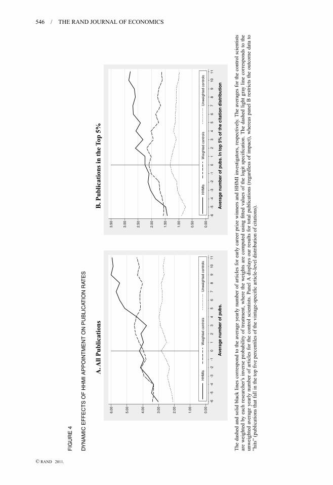
Figure 4 display the time path of the average publication count and top 5% outcome forHHMIs and ECPWs separately. While computing the averages, we weight each control scientist’soutcome by his/her inverse probability of being selected into the program, while leaving thetreated scientists’ outcomes unchanged. Loosely, Figures 4A and 4B provide a graphical intuitionfor the SDD estimates: they correspond to the difference between the change in outcomes forthe HHMI investigators and for a pseudopopulation of control scientists matched on observables.A necessary condition for the plausibility of this exercise is that the treated and control groupsdisplay parallel output trends prior to the appointment event. This appears to be the case here.

Interestingly, for three years after appointment, the outcomes for treated and control scientistscontinue to track each other closely. Figure 4B even suggests that the control group (appropriatelyselected on observables) briefly outpaces the treatment group following the appointment,consistent with Manso’s (2011) theory which predicts both slower and more variable returnsunder an exploration incentive scheme. This difference is not statistically significant, however,which is perhaps unsurprising given our sample’s relatively small size. HHMI investigators’output begins to diverge from that of ECPWs only four to five years after appointment, and thisdivergence is more marked in Figure 4B.

We have explored the hypothesis of a temporary, post-appointment slowdown qualitativelyby asking eight current and former HHMI investigators about the “retooling” necessary to takeadvantage of the freedom afforded by the program. This idea resonated with these scientists, butit also seems clear that these lags are very heterogeneous across labs. Some of them mentionedwaiting until their first renewal before branching out; others were clearly itching to begin newprojects, for example by focusing on a new disease (autism vs. Huntington’s), model organism(mice vs. yeast), or discipline (chemistry vs. cell biology). Still others described a less deliberateexploration process whereby the logic of their traditional research projects opened up novelopportunities, which they could more easily take advantage of as HHMI investigators.

� Effects of HHMI appointment on failure. It seems intuitive that exploration wouldlead scientists to “strike out” more often. Measuring failure is difficult, because it might leadresearchers to abort projects altogether. Here we ask whether HHMI investigators produce more

16 Because the Poisson model is in the linear exponential family, the coefficient estimates remain consistent as longas the mean of the dependent variable is correctly specified (Wooldridge, 1996; Santos Silva and Tenreyro, 2006). Further,‘robust’ standard errors are consistent even if the underlying data-generating process is not Poisson.

C© RAND 2011.


FIG

UR

E4

DY

NA

MIC

EF

FE

CT

SO

FH

HM

IAP

PO

INT

ME

NT

ON

PU

BLI

CAT

ION

RAT

ES

A. A

ll P

ublic

atio

nsB

. Pub

licat

ions

in t

he T

op 5

%

0.00

1.00

2.00

3.0

0

4.00

5.0

0

6.0

0

-6-5

-4-3

-2-1

01

23

45

67

89

1011

Ave

rag

e n

um

ber

of

pu

bs.

HH

MIs

Wei

ghte

d co

ntro

lsU

nwei

ghte

d co

ntro

ls0.

00

0.50

1.00

1.50

2.00

2.50

3.00

3.50

-6-5

-4-3

-2-1

01

23

45

67

89

1011

Ave

rag

e n

umbe

r of

pu

bs.

In t

op

5%

of

the

cita

tio

n d

istr

ibu

tion

HH

MIs

Wei

ghte

d co

ntro

lsU

nwei

ghte

d co

ntro

ls

The

dash

edan

dso

lid

blac

kli

nes

corr

espo

ndto

the

aver

age

year

lynu

mbe

rof

arti

cles

for

earl

yca

reer

priz

ew

inne

rsan

dH

HM

Iin

vest

igat

ors,

resp

ectiv

ely.

The

aver

ages

for

the

cont

rol

scie

ntis

tsar

ew

eigh

ted

byea

chre

sear

cher

’sin

vers

epr

obab

ilit

yof

trea

tmen

t,w

here

the

wei

ghts

are

com

pute

dus

ing

fitt

edva

lues

ofth

elo

git

spec

ifica

tion

.T

heda

shed

ligh

tgr

ayli

neco

rres

pond

sto

the

unw

eigh

ted

aver

age

year

lynu

mbe

rof

arti

cles

for

the

cont

rol

scie

ntis

ts.

Pane

lA

disp

lays

our

resu

lts

for

tota

lpu

blic

atio

ns(r

egar

dles

sof

impa

ct),

whe

reas

pane

lB

rest

rict

sth

eou

tcom

eda

tato

”hit

s”(p

ubli

cati

ons

that

fall

inth

eto

pfi

vepe

rcen

tile

sof

the

vint

age-

spec

ific

arti

cle-

leve

ldis

trib

utio

nof

cita

tion

s).

C© RAND 2011.


TABLE 7 Effects of HHMI Appointment on NIH Funding

Dependent Variable “Naive” X-Section ATE ATT DD SDD

NIH funding ($) −0.404∗∗ −0.549∗∗ −0.497∗∗ −0.546∗∗ −0.426∗∗

(0.095) (0.099) (0.094) (0.105) (0.115)No. of R01 Apps. −0.521∗∗ −0.603∗∗ −0.486∗∗

(0.122) (0.126) (0.122)Avg. priority score for R01 −0.077∗∗ −0.075∗∗ −0.057†

(0.029) (0.025) (0.032)

No. of scientists 417 417 417 417 417

Note: Each coefficient corresponds to the treatment effect of HHMI appointment in a specification that regressesthe dependent variable on treatment status, five age indicator variables (5–10 years of career age, 10–15 years, 15–20years, 20–25 years, and 25 years and more of career age), and year indicator variables. The cross-sectional models(corresponding to the first three columns) also include three lab indicator variables, a gender indicator variable, andtwo degree-type indicator variables (coefficients not reported). Estimates derive from QML Poisson estimation, withrobust standard errors in parentheses, clustered around scientist (X-section, ATE, ATT, and DD columns); bootstrappedstandard errors are reported for the semiparametric difference-in-differences estimates. All specifications except the naivecross-sections and the plain difference-in-differences include regression weights computed using fitted values for theprobability of HHMI appointment estimated in Table 5. The weights differ depending on whether ATT or ATE is theeffect of interest, and whether the focus is on generating a between-scientist comparison (ATE & ATT columns) or awithin-scientist comparison (SDD column). Because grant application data are only available for the period 2003–2008,the determinants of application rates and priority scores are estimated using a single cross-section that pools together allof the data for the corresponding period. See Section 4 for more details.

†p < 0.10, ∗p < 0.05, p < 0.01.

articles of little import, relative to controls. To answer this question, we examine whether HHMIappointment increases the rate of publications that fall in the bottom quartile of citations. Relativeto ECPW scholars, HHMI investigators indeed fail more often, regardless of estimation method;some of these estimates are large in magnitude, but they are also imprecisely estimated. The lackof statistical significance is not terribly surprising, because relatively few of the articles producedby these elite scientists will fail to garner the three citations that correspond to the 25th percentileof the citation distribution in most years.

An alternative approach is to use these scientists’ own citation impact prior to appointmentto assess their performance in the post-appointment regime, rather than a universal citationbenchmark as above. The corresponding results are displayed in the last two lines of Table 6.The coefficient estimates pertain to the HHMI treatment effect in cross-sectional comparisonswhere the rates of “hit” and “flop” publications are modelled using quasi-maximum likelihoodPoisson. To compute the number of hits, we count the number of times each scientist publishes anarticle whose citation quantile places it above the highest citation quantile of any article publishedprior to appointment. Symmetrically, the number of flops is computed by counting the number oftimes each scientist publishes an article whose citation quantile places it below the lowest citationquantile of any article published prior to appointment (further details are provided in AppendixD). Because we use citation data for the entire pre-appointment period to compute individualcitation benchmarks, there are no DD and SDD specifications for these two outcomes.

We find robust statistical evidence that HHMI appointment increases the frequency of bothhits and flops. We focus on the latter result, because an increased rate of failure under anexploration incentive scheme is a strong prediction of the theory. It is also more challenging toreconcile with the view that HHMI simply picks extraordinarily talented scientists and then takescredit for their accomplishments. Of course, we cannot rule out a more nuanced selection storywhereby the elite scientists who serve as judges in HHMI competitions are skilled at identifyingscientists destined to push the scientific frontier outward.

� Effects of HHMI appointment on NIH grant outcomes. In Table 7, we document anegative association between HHMI appointment and NIH funding that holds both in the cross-sectional and the within-scientist dimensions of the data. This effect corresponds in large part to

C© RAND 2011.


TABLE 8 Effects of HHMI Appointment on the Direction of Research

Impact of Treatment on: Dependent Variable X-Section ATE ATT DD SDD

Topic novelty Avg. MeSH keyword age −0.028∗∗ −0.014 − 0.016† −0.020 −0.027∗

(0.009) (0.009) (0.009) (0.013) (0.013)Change in research Normalized MeSH −0.258∗∗ −0.206∗∗ −0.259∗∗

direction keyword overlap (0.060) (0.058) (0.059)Breadth of impact Citing journal diversity index 0.223∗∗ 0.192∗∗ 0.231∗∗

(0.071) (0.060) (0.073)

No. of scientists 417 417 417 417 417

Note: For the analysis of the determinants of topic novelty, each coefficient corresponds to the treatment effect ofHHMI appointment in a specification that regresses measures of scientific novelty on treatment status, five age indicatorvariables (5–10 years of career age, 10–15 years, 15–20 years, 20–25 years, and 25 years and more of career age),and year indicator variables in all models. The cross-sectional models (corresponding to the first three columns) alsoinclude three lab indicator variables, a gender indicator variable, and two degree-type indicator variables (coefficients notreported). Estimates derive from QML Poisson estimation, with robust standard errors in parentheses, clustered aroundscientist (X-section, ATE, ATT, and DD columns); bootstrapped standard errors are reported for the semiparametricdifference-in-differences estimates.

For the other two outcomes (keyword overlap and diversity of citing journals), each coefficient corresponds to thetreatment effect of HHMI appointment on various measures of an investigator’s scientific direction in the “after” period(1995–2006). All models include as independent variables year of highest degree indicator variables, three lab typeindicator variables, a gender indicator variable, and two degree-type indicator variables (coefficients not reported). Alsoincluded is an offset for the dependent variable in the “before” period (1986–1994). Because all of the dependent variableare bounded inclusively by 0 and 1, estimates stem from a QML fractional logit procedure (Papke and Wooldridge, 1996),with robust standard errors in parentheses. All specifications except the naive cross-sections and the plain difference-in-differences include regression weights computed using fitted values for the probability of HHMI appointment estimatedin Table 5. The weights differ depending on whether ATT or ATE is the effect of interest; and whether the focus is ongenerating a between-scientist comparison (ATE and ATT columns), or a within-scientist comparison (SDD column).See Section 4 for more details.

†p < 0.10, ∗p < 0.05, ∗∗p < 0.01.

a mechanical substitution of HHMI resources for traditional NIH funding: the number of R01grant applications by HHMI investigators is, on average, only about 60% of the correspondingnumber for ECPW scholars. But application behavior does not on its own explain the declinein NIH funding; conditional on applying, applications from HHMI scientists receive higherpriority scores (i.e., are judged more harshly by study sections). When combined with the resultspertaining to citation impact, this evidence supports the view that the punctiliousness of the NIHpeer-review process crowds out scientific exploration.17

� Effects of HHMI appointment on the direction of research. So far, our presentation ofresults has conflated intensity of exploration with the rate at which tail outcomes are produced.But taken literally, the Manso (2011) model does not predict that “pay-for-future performance”incentives will result in better outcomes; it simply asserts that agents subject to those incentiveswill increase their rates of exploration, relative to agents who receive piece rates. This is thehypothesis we examine in Table 8. Choosing less-traveled scientific avenues could also leavetrails in the content of what scientists publish, and in particular affect the keywords that tag theirpublications. We first focus on whether HHMI investigators are prone to define the scientificfrontier, by examining the vintage of the MeSH keywords in their output. In our analysis, akeyword is born the earliest year in which it appears in any publication indexed by PubMed.We then compute the average age of all keywords or all keyword pairs in each scientist’s yearlyoutput. Table 8 shows that HHMI investigators indeed tackle more novel topics; the coefficientestimates are negative regardless of estimation method.

Next, we ask whether evidence exists that HHMI investigators alter the direction of theirscientific trajectory following their appointment. We first examine the program’s effect on the

17 More prosaically, they might put less effort into preparing these proposals, because they benefit from the safetyof Hughes funding.

C© RAND 2011.


number of unique publication keywords that overlap between the set of articles published in the“before” period (1986–1994) and the “after” period (1998–2006). This measure is then normalizedby the number of unique keywords used in the after period. For each control group, we reportboth the results of a “naive” specification and the results of two specifications which incorporateinverse probability of treatment weights corresponding to ATE and ATT. Because the dependentvariable is a proportion, we estimate these models using the quasi-maximum likelihood fractionallogit estimator of Papke and Wooldridge (1996). Relative to ECPW scholars, HHMI investigatorsexhibit unambiguously lower overlap in keyword use. The effects are statistically significant, andimply that HHMI appointment is associated with about a 10% lower rate of overlap.

Our last test focuses on the breadth—rather than the depth—of impact for these scientists’publications. To do so, we examine the journals in which citing articles appear, and compute theHerfindahl of journal concentration H . We find that HHMI investigators exhibit higher levelsof (1 − H) in the post-appointment period, that is, their work is cited by a more diverse set ofjournals than the articles published by ECPWs. Overall, the results in Table 8 are consistent withthe idea that HHMI investigators broaden their research agenda in the post-appointment period,a necessary condition for exploration.

� Incentives versus alternative mechanisms. Even if our estimates of HHMI appointments’treatment effects can be given a causal interpretation, ascribing them to the program’s incentivefeatures requires an interpretive leap.

First, we are unable to ascertain the extent to which the program increases productivity ratherthan output. It is hard to compare directly HHMI and NIH levels of funding, because the twoprograms are structured in a different fashion.18 Yet, it appears likely that, per dollar of funding,HHMI investigators do not publish more articles than researchers funded by the NIH. Of course,if the supply of genuinely creative ideas is very inelastic, then publications per dollar of fundingwill not adequately measure researchers’ productivity.19 We also note that the results pertainingto the diversity of experimentation are less vulnerable to this critique, because they essentiallyhold output constant.

Second, the prestige conferred by HHMI appointment might have independent effects onscientists’ achievements, either by increasing exposure to their research or through a dynamic ofascription that has long been the focus of sociologists of science (Merton, 1968). Azoulay, Stuart,and Wang (2010) provide estimates of the HHMI investigator program’s “anointment effects” byexamining whether appointment shifts the citation rate of articles written in the pre-appointmentperiod; their evidence points to effects of very modest magnitude. As such, an interpretation ofour results that emphasizes the status benefits of HHMI appointment appears unwarranted.

Third, collaboration between scientists in the treatment and control groups might threaten thevalidity of the comparisons drawn in the analysis. Fifty-nine out of the 73 HHMI investigators haveat least one control collaborator; 10 have five or more. However, peer effects from coauthorship(e.g., Azoulay, Graff Zivin, and Wang, 2010), which enhance the accomplishments of the controlgroup, would tend to dampen the magnitudes of the effects estimated above.

A more subtle reinterpretation of our main results is that “explorer types” are more likely toseek HHMI appointment. A sorting process in this vein would imply that the freedom and long-term funding bundled with HHMI appointment have real effects, even if they do not really inducebehavioral changes in the treated group. However, a peculiar feature of the HHMI appointmentprocess is that candidates do not apply but rather are nominated by their universities, which areendowed by HHMI with a very limited number of nomination slots. This casts doubt on the

18 For example, HHMI does not pay host institutions standard overhead rates, but does make a contribution towardrent and occupancy.

19 In a recent article, Jacob and Lefgren (2007) estimate that the elasticity of citations with respect to NIH R01grant funding is quite small in magnitude, and often insignificantly different from 0. Given their regression-discontinuitydesign, it would be hazardous to import their estimate for the analysis of the scientist population analyzed in the presentstudy.

C© RAND 2011.


sorting interpretation at the principal investigator level. It is altogether more likely (and also morefeasible) for talented postdoctoral researchers and graduate students with idiosyncratic tastes forexploration to sort themselves into HHMI-funded labs. The fact that HHMI labs train a muchhigher number of young scientists who go on to win early career prizes is consistent with a sortingprocess at the level of trainees.

In summary, we argue the differences observed between HHMI investigators and controlsare likely to be driven by the program’s distinct incentive features, as opposed to other potentialeffects of HHMI appointment.

6. Conclusion

� In this article, we exploit key differences across funding streams within the academiclife sciences to examine the impact of incentives embodied in research contracts on the rate ofscientific exploration. We find that selection into the HHMI investigator program—which rewardslong-term success, encourages intellectual experimentation, and provides rich feedback to itsappointees—leads to higher levels of breakthrough innovation, compared with NIH funding—which is characterized by short grant cycles, predefined deliverables, and unforgiving renewalpolicies. Moreover, the magnitudes of these effects are quite large.

Our findings are important for at least two reasons. First, they demonstrate the impact ofnuanced features of research contracts for the rate and direction of scientific progress. Given theprominent role that scientific change is presumed to play in the process of economic growth (e.g.,Mokyr, 2002), this has important implications for the organization of public and private researchinstitutions. Second, they offer empirical support for the theoretical model developed by Manso(2011), and as such may provide insights relevant to a wider set of industries that rely on creativeprofessionals, ranging from advertising and computer programming to leadership roles at theupper echelons of the corporate world.

Finally, our results should not be interpreted as a critique of NIH and its funding policies.Although “exploration” incentive contracts appear to stimulate creativity in this setting, it isunclear how easily, and at what cost, the program could be scaled up. Only scientists showingexceptional promise are eligible for HHMI appointment, and our results may not generalize tothe overall population of scientists eligible for grant funding, which includes gifted individualsas well as those with more modest talent. Moreover, HHMI provides detailed evaluation andfeedback to its investigators. The richness of this feedback consumes a great deal of resources,particularly the time of the elite scientists who serve on review panels, and its quality mightdegrade if the program were expanded drastically.

It is also vital to recognize that NIH operates under political constraints that a privatefoundation like HHMI can safely ignore. For instance, all public research agencies need to spreadtheir support across many institutions, including those of lesser renown. Similarly, supportingindividual projects, rather than individual scientists, introduces a level of impersonality in thefunding decisions that may make them easier to defend vis-a-vis congressional appropriators.

Much more could be done to explore the impacts of contract design on research output inthis setting. For example, does the quality of peers at these investigators’ institutions temper ormagnify these effects? Do the effects of exploration-style incentives exhibit hysteresis, that is,do they lead scientists to be more creative under more conventional contractual arrangements?Answering these questions is the next step of our research agenda.

Appendix AFunding people versus funding specific projects

We develop a simple model to contrast the “specific project” and the “people, not projects” approaches to scientificfunding. The researcher lives for two periods. In each period, she chooses a project i ∈ I, producing output S (“success”)with probability pi or output F (“failure”) with probability 1 − pi. The probability pi of success when the researcherchooses project i may be unknown. To obtain information about pi, she must engage in experimentation. We let E[pi]

C© RAND 2011.


denote the unconditional expectation of pi, E[pi | S, j] denote the conditional expectation of pi given a success on projectj, and E[pi | F, j] denote the conditional expectation of pi given a failure on project j.

When the researcher chooses project i ∈ I, she only learns about the probability pi, so that

E[p j ] = E[p j |S, i] = E[p j |F, i] for j �= i .

The central concern that arises is the tension between exploration of new ideas and the exploitation of already-existing ideas along conventional lines (March, 1991). To focus on the tension between exploration and exploitation, weassume that in each period the researcher chooses between two projects. Project 1, the “conventional” research project,has a known probability p1 of success such that

p1 = E[p1] = E[p1|S, 1] = E[p1|F, 1].

Project 2, the innovative research project, has an unknown probability p2 of success such that

E[p2|F, 2] < E[p2] < E[p2|S, 2].

We assume that the innovative research project is of an exploratory nature. This means that when the researcherexperiments with the innovative research project, she is initially not as likely to succeed as when she takes a well-troddenpath, as is the case with the conventional research project. However, if she succeeds with the innovative project, sheupdates her beliefs about p2, so that choosing the innovative project becomes perceived as superior to choosing theconventional project. This is captured by

E[p2] < p1 < E[p2|S, 2]. (A1)

The researcher is risk neutral and has a discount factor normalized to one. Her objective function R assigns someweight α to the outcome produced by this research as well as some weight to her private preferences between the twoprojects. These private preferences are represented with a cost ci that is incurred by the researcher whenever she pursuesproject i. The researcher thus chooses an action plan 〈i

jk 〉 to maximize her total expected payoff:

R(〈ijk 〉) = {E[pi ]S + (1 − E[pi ])F − ci } + E[pi ]{E[p j |S, i]S + (1 − E[p j |S, i])F − c j }

+ (1 − E[pi ])(E[pk |F, i]S + (1 − E[pk |F, i])F − ck), (A2)

where i is the first-period action, j is the second-period action in case of success in the first period, and k is the second-period action in case of failure in the first period. We assume that the researcher gets enough funding to perform researchduring the two periods. We consider two funding mechanisms: the “specific project” approach and the “people, notprojects” approach.

� The “specific project” approach. Under this approach, the researcher must choose one project to submit forfunding and must work on that project during the two periods. Two action plans need to be considered: 〈1 1

1 〉 and 〈2 22 〉. If

the researcher chooses action plan 〈1 11 〉, his total expected payoff is

R(〈1 11 〉) = {E[p1]S + (1 − E[p1])F − c1} + E[p1]{E[p1]S + (1 − E[p1])F − c1}

+ (1 − E[p1]){E[p1]S + (1 − E[p1])F − c1}. (A3)

If the researcher chooses action plan 〈2 22 〉, his total expected payoff is

R(〈2 22 〉) = {E[p2]S + (1 − E[p2])F − c2} + E[p2]{E[p2|S, 2]S + (1 − E[p2|S, 2])F − c2}

+ (1 − E[p2]){E[p2|F, 2]S + (1 − E[p2|F, 2])F − c2}. (A4)

From Bayes’ rule, the payoff R(〈2 22 〉) is higher than the payoff R(〈1 1

1 〉) if and only if

α(E[p2] − p1)(S − F) ≥ (c2 − c1). (A5)

� The “people, not projects” approach. Under this approach, the researcher can choose any of the two projectsin each period. Two action plans need to be considered: 〈1 1

1 〉, 〈2 21 〉. If the researcher chooses action plan 〈1 1

1 〉, her totalexpected payoff is

R(〈1 11 〉) = {E[p1]S + (1 − E[p1])F − c1} + E[p1]{E[p1]S + (1 − E[p1])F − c1}

+ (1 − E[p1]){E[p1]S + (1 − E[p1])F − c1}. (A6)

If the researcher chooses action plan 〈2 21 〉, her total expected payoff is

R(〈2 21 〉) = {E[p2]S + (1 − E[p2])F − c2} + E[p2]{E[p2|S, 2]S + (1 − E[p2|S, 2])F − c2}

+ (1 − E[p2]){E[p1]S + (1 − E[p1])F − c1}. (A7)

C© RAND 2011.


The payoff R(〈2 21 〉) is higher than R(〈1 1

1 〉) if and only if

α{E[p2](E[p2|S, 2] − p1) + (E[p2] − p1)}(S − F) ≥ (1 + E[p2])(c2 − c1). (A8)

The following proposition contrasts exploration under “specific project” funding and “people, not projects” funding.

Proposition 1. If the agent explores under “specific project” funding, he also explores under “people, not projects”funding. However, there are situations in which the agent explores under “people, not projects” funding but exploits under“specific project” funding.

Proof . The first statement follows from the fact that (A5) implies (A8). For the second statement, we construct thefollowing example. If c2 > c1, (A5) implies that the agent never explores under the “specific project” approach. However,from (A8), if the payoff from exploration is sufficiently high, the agent will explore under the “people, not projects”approach.

Appendix BCareer and output data

For every scientist in the control or treatment group, we collected career information from three sources: original CVs/NIHbiosketches; Who’s Who profiles; and Google searches. In practice, the combination of these approaches enabled us tofind employment and demographic data for all the investigators considered in the article. Matching these individuals withNIH grant information is not challenging because both full names and institutional affiliations can be used. Getting aprecise tally of publications at the individual level is more involved. We will describe this process using as an exampleMario Capecchi, the Nobel Prize winner (and HHMI investigator) mentioned in the Introduction.

The matching process begins with the creation of a customized PubMed search query for each scientist. In thecase of Capecchi, the query is ((‘‘capecchi mr’’[au] OR ‘‘capecchi m’’[au]) NOT 7816017[pmid] AND

1966:2006[dp]), and it returns 122 original publications (the query also returns 19 letters, editorials, interviews,reviews, etc., which we ignore). The process of harvesting bibliomes from PubMed using name variations and queries asinputs is facilitated by the use of PubHarvester, a software program we specifically designed for this purpose (Azoulay,Stellman, and Graff Zivin, 2006).

Capecchi’s PubMed query accounts for his inconsistent use of the middle initial, but is otherwise quite simple.For other scientists, queries might factor in their inconsistent use of the suffix “Jr.” or name variations coincident withchanges in marital status. For yet many others with common names, the queries are more involved, and make use of CVinformation such as scientific keywords, institutional affiliation, frequent coauthors’ names, and so forth. This degreeof labor-intensive customization ensures that a scientist’s bibliome excludes publications belonging to homonymousscientists.

Appendix CEstimation procedure for the semiparametric DD estimates

The ATE, ATT, and DD effects stem from panel specifications; the sample size is equal to the total number of independentcareer years for each scientist (N × T = 8,767). The procedure followed to estimate the SDD effects is slightly different.We first regress the various measures of output on calendar year and age indicator variables using the full panel, andcompute the residuals εit. In a second step, we sum the residuals corresponding to the pre-appointment (1986–1994)and post-appointment (1998–2006) periods separately for each scientist. In the final step, the SDD effects are obtainedby regressing

∑1994t=1986 εit − ∑

2006t=1998 εit on treatment status, weighting these differences as described in Section 4. Note

that the sample size corresponds in this case to the number of scientists (N = 417), not the number of scientist-yearobservations.

Appendix DScientist-specific citation benchmarks

We illustrate the computation of the number of hits and flops using the example of Iva Greenwald, an HHMI investigatorfrom Columbia University. Prior to 1994 (the year of her appointment), her publication with the highest citation quantileis an article which appeared in the journal Cell in 1993 (341 citations as of the end of 2008, which places it in the toppercentile of the article-level distribution). Conversely, her publication with the lowest citation quantile is an article whichappeared in the journal Molecular and Cellular Biology, also in 1993. It garnered only 11 citations, which places it atthe 52nd percentile of the distribution. Between 1995 and 2006, Greenwald published three more publications in the toppercentile of the citation distribution, given their vintage. And she published three more publications which fell in the32nd, 44th, and 50th percentiles of the distribution in the years they were published. As a result, both the number of hits,and of flops, are equal to three for this investigator.

C© RAND 2011.


� Estimation. Because we use the entire pre-appointment data to compute citation benchmarks specific to eachindividual scientist, we can only analyze the effect of HHMI appointment on these measures of impact using the cross-sectional dimension of the data, collapsing all post-appointment years into a single observation for each scientist. For thenumber of flops, the equation we estimate can be written

E[FLOPSi | Xi ] = exp(β0 + β1HHMIi + β′2 Zi + β3MIN QNTLi + φ(SCIENTIST AGEi )), (D1)

where HHMI denotes the treatment effect, the variables in Z include degree type, lab type, and gender indicator variables,MIN QNTL is the citation quantile corresponding to scientist i’s least impactful article published prior to appointment,20

and φ(SCIENTIST AGEi ) is a flexible function of scientist i’s career age—in practice a full set of indicator variables for thedifferent years in which our scientists received their highest degree. Estimation proceeds by quasi-maximum likelihood.In some of the specifications, the data are weighted to reflect each scientist’s inverse probability of being appointed to theprogram, as explained in Section 4.

References

ABADIE, A. “Semiparametric Difference-in-Differences Estimators.” Review of Economic Studies, Vol. 72 (2005),pp. 1–19.

AGHION, P., DEWATRIPONT, M., AND STEIN, J.C. “Academic Freedom, Private Sector Focus, and the Process of Innovation.”RAND Journal of Economics, Vol. 39 (2008), pp. 617–635.

AMABILE, T.M. Creativity in Context. Boulder, CO: Westview Press, 1996.AZOULAY, P., STELLMAN, A., AND GRAFF ZIVIN, J. “PublicationHarvester: An Open-Source Software Tool for Science

Policy Research.” Research Policy, Vol. 35 (2006), pp. 970–974.———, GRAFF ZIVIN, J. AND WANG, J. “Superstar Extinction.” Quarterly Journal of Economics, Vol. 125 (2010),

pp. 549–589.———, STUART, T., and WANG, Y. “Matthew: Effect or Fable?” Working Paper, MIT Sloan School of Management, 2010.

Available at http://pazoulay.scripts.mit.edu/BURT, R.S. “Structural Holes and Good Ideas.” American Journal of Sociology, Vol. 110 (2004), pp. 349–399.BUSSO, M., DINARDO, J., AND MCCRARY, J. “Finite Sample Properties of Semiparametric Estimators of Average Treatment

Effects.” Working Paper, University of Michigan, 2008.CAPECCHI, M.R. “Response.” Science, Vol. 319 (2008), pp. 900–901.CHARLTON, B.G. “Why Are Modern Scientists So Dull? How Science Selects for Perseverance and Sociability at the

Expense of Intelligence and Creativity.” Medical Hypotheses, Vol. 72 (2009), pp. 237–243.DEHEJIA, R.H. AND WAHBA, S. “Propensity Score-Matching Methods for Nonexperimental Causal Studies.” Review of

Economics and Statistics, Vol. 84 (2002), pp. 151–161.EDERER, F. AND MANSO, G. “Is Pay-for-Performance Detrimental to Innovation?” Working Paper, MIT Sloan School of

Management, 2010.HIRANO, K. AND IMBENS, G.W. “Estimation of Causal Effects Using Propensity Score Weighting: An Application to Data

on Right Heart Catherization.” Health Services & Outcomes Research Methodology, Vol. 2 (2001), pp. 259–278.HOLMSTROM, B. “Agency Costs and Innovation.” Journal of Economic Behavior and Organization, Vol. 12 (1989), pp.

305–327.JACOB, B. AND LEFGREN, L. “The Impact of Research Grant Funding on Research Productivity.” Working Paper no. 13519,

NBER, 2007.KAPLAN, D. “How to Improve Peer Review at NIH.” Scientist, Vol. 19 (2005), p. 10.KOLATA, G. “Grant System Leads Cancer Researchers to Play It Safe.” New York Times, June 28, 2009.LAZEAR, E. “Performance Pay and Productivity.” American Economic Review, Vol. 90 (2000), pp. 1346–1361.LERNER, J. AND WULF, J. “Innovation and Incentives: Evidence from Corporate R&D.” Review of Economics and Statistics,

Vol. 89 (2007), pp. 634–644.LOTKA, A.J. “The Frequency Distribution of Scientific Productivity.” Journal of the Washington Academy of Sciences,

Vol. 16 (1926), pp. 317–323.MANSO, G. “Motivating Innovation.” Journal of Finance, Vol. 66 (2011).MARCH, J.G. “Exploration and Exploitation in Organizational Learning.” Organization Science, Vol. 2 (1991), pp. 71–87.MCKNIGHT, S.L. “Unconventional Wisdom.” Cell, Vol. 138 (2009), pp. 817–819.MERTON, R.K. “The Matthew Effect in Science.” Science, Vol. 159 (1968), pp. 56–63.MOKYR, J. The Gifts of Athena. Princeton, NJ: Princeton University Press, 2002.PAPKE, L.E. AND WOOLDRIDGE, J.M. “Econometric Methods for Fractional Responses with an Application to 401(k) Plan

Participation Rates.” Journal of Applied Econometrics, Vol. 11 (1996), pp. 619–632.ROBINS, J.M. AND ROTNITZKY, A. “Semiparametric Efficiency in Multivariate Regression Models with Missing Data.”

Journal of the American Statistical Association, Vol. 90 (1995), pp. 122–129.

20 In the case of hits, the corresponding specification includes M AX QN T L—the citation quantile correspondingto scientist i’s most impactful article published prior to appointment—as an independent variable.

C© RAND 2011.


ROSENBAUM, P.R. AND RUBIN, D.B. “The Central Role of the Propensity Score in Observational Studies for Causal Effects.”Biometrika, Vol. 70 (1983), pp. 41–55.

RUBIN, D.B. “Characterizing the Estimation of Parameters in Incomplete-Data Problems.” Journal of the AmericanStatistical Association, Vol. 69 (1974), pp. 467–474.

SANTOS SILVA, J.M.C. AND TENREYRO, S. “The Log of Gravity.” Review of Economics and Statistics, Vol. 88 (2006),pp. 641–658.

SAUERMANN, H. AND COHEN, W.M. “What Makes Them Tick? Employee Motives and Firm Innovation.” ManagementScience, Vol. 56 (2010), pp. 2134–2153.

SIMONTON, D.K. Creativity in Science: Chance, Logic, Genius, and Zeitgeist. New York: Cambridge University Press,2004.

SMITH, J.A. AND TODD, P.E. “Does Matching Overcome LaLonde’s Critique of Nonexperimental Estimators?” Journal ofEconometrics, Vol. 125 (2005), pp. 305–353.

TIAN, X. AND WANG, T.Y. “Tolerance for Failure and Corporate Innovation.” Working Paper, Indiana University, 2010.WEITZMAN, M. Recombinant growth, Quarterly Journal of Economics, Vol. 13(1998), pp. 331–360.WOOLDRIDGE, J.M. “Quasi-Likelihood Methods for Count Data.” In M.H. Pesaran and P. Schmidt, eds., Handbook of

Applied Econometrics, Vol 2. Oxford: Blackwell, 1996.———, “Inverse Probability Weighted M-Estimators for Sample Selection, Attrition, and Stratification.” Portuguese

Economic Journal, Vol. 1 (2002), pp. 117–139.

C© RAND 2011.

Documents

Incentives and creativity: evidence from the academic life