Temporary Investment Tax Incentives:

Theory with Evidence from Bonus Depreciation

Christopher L. House

University of Michigan

and

Matthew D. Shapiro

University of Michigan and NBER

September 28, 2004

We gratefully acknowledge the comments of William Gale, James Hines, Peter Orszag, Samara Potter, Dan Silverman and Joel Slemrod.

Temporary Investment Tax Incentives:

Theory with Evidence from Bonus Depreciation

ABSTRACT This paper considers the economy’s reaction to a temporary investment tax subsidy. Because the eventual payoff from acquiring a long-lived capital good is unrelated to the date of purchase or installation, there are powerful incentives to delay or accelerate investment to take advantage of predictable intertemporal variations in cost. For these goods, the elasticity of investment demand is nearly infinite. Consequently, for a temporary tax change, the shadow price of long-lived capital goods fully reflects the tax subsidy regardless of the elasticity of investment supply. While price data provide no information on the elasticity of supply, they reveal the extent to which adjustment costs are internal or external to the firm. The elasticity of investment supply can be inferred from quantity data alone. The bonus depreciation allowance passed in 2002 and increased in 2003 provides a sharp test of the theory. In the law, certain types of long-lived capital goods qualify for substantial tax subsides while others do not. The data show that investment in capital that qualified for the subsidy was substantially higher than capital that did not. The adjustment cost parameters implied by the data are in line with estimates from earlier studies. Market prices do not react to the subsidy, which suggests that internal adjustment costs are important for investment decisions. Even though the policy increased spending on types of equipment that benefited substantially from bonus depreciation, the aggregate effects of the policy were modest. The calculations suggest that the policy may have increased output by roughly 0.1% in 2003 and 2004 and increased employment by roughly 100,000 jobs. Output, employment, and investment will fall in 2005 when the policy expires.

Christopher L. House Matthew D. Shapiro Department of Economics Department of Economics University of Michigan University of Michigan Ann Arbor MI 49109-1220 Ann Arbor MI 48109-1220 tel. 734 764-2364 and NBER chouse@umich.edu tel. 734 764-5419 shapiro@umich.edu

I. INTRODUCTION

The U.S. economy is now in the wake of three major tax changes: the Economic Growth

and Tax Relief Reconciliation Act of 2001 (EGTRRA), the Job Creation and Worker

Assistance Act of 2002 (JCWAA), and the Jobs and Growth Tax Relief Reconciliation Act

of 2003 (JGTRRA). In academic journals, in policy briefs, and in the popular press, there

has been and continues to be much more emphasis on the 2001 and 2003 laws. This is no

accident. The 2001 and 2003 laws have much bigger price tags than the 2002 law. The

cumulative loss in revenue attributed to EGTRRA in the ten years after its passage is

roughly $1.3 trillion. The ten-year revenue shortfall attributed to JGTRRA is $350

billion. In comparison, the 2002 tax bill reduces revenue by only about $40 billion over

ten years.

Another reason that the 2001 and 2003 laws got so much public attention is that

these laws made tax changes that were easily understood—reductions in tax rates, the

increased child tax credit, reductions in the estate tax, and so on. The main provision of

the 2002 tax bill was an accelerated depreciation allowance for businesses. In 2003,

JGTRRA further accelerated depreciation allowances.

Yet, even though JCWAA offered a relatively small tax cut to businesses, the tax

cut applies to something that is potentially very sensitive to such changes: the timing of

investment. There are good reasons to believe that the decision to invest should respond

sharply to even modest changes in after-tax costs, especially those that are temporary.

This paper presents a general equilibrium analysis of temporary changes in taxes

that affect the incentive to invest. Though the paper is motivated by recent changes in tax

law, the analysis has general implications for the equilibrium effects of temporary tax

incentives. Several results flow from a basic property of investment decisions: If firms

are sufficiently forward-looking and investment goods are sufficiently long-lived, the

elasticity of investment demand is nearly infinite with respect to temporary variations in

cost. This property rests directly on the forward-looking nature of investment. Since the

value of such an investment is anchored by long-run factors, variations in the timing of

these investments have only minor consequences for their eventual payoffs. As a result,

2

the decision of when to invest is highly sensitive to temporary variations in short-run

costs.

This insight leads to several results concerning temporary investment tax

incentives. First, if the supply of investment goods is highly elastic in the short run, the

quantity of investment will react dramatically to such policies. Second, temporary tax

changes are necessarily accompanied by offsetting changes in the pre-tax shadow price of

investment goods. Indeed, we will show that in equilibrium, regardless of the elasticity

of the flow supply of investment goods, the pre-tax shadow price of investment goods

must move one-for-one with the tax subsidy. Because prices increase by the same

amount regardless of the elasticity of supply, observing price increases following a

temporary tax incentive is not evidence that the supply of investment is relatively

inelastic.

To complicate matters, observed market prices may only partially reflect the

subsidy. Because the shadow price of capital includes costs that are both internal and

external to the firm, the observed increases in market prices are bounded above by the

size of the tax incentive. Thus, while price data are not informative about the elasticity of

supply, price data can provide information about the composition of internal versus

external costs of investment. If pre-tax prices only partially reflect the subsidy then a

significant part of the cost of investment must be internal.

The elasticity of investment supply does matter for the equilibrium determination

of quantity. Because economic theory dictates that the underlying shadow price of

investment moves one-for-one with a temporary tax subsidy, the effective elasticity of

supply can be inferred from data on quantity alone.

We test the theory by examining disaggregate investment data following the 2002

and 2003 tax bills. These bills provided temporarily accelerated depreciation, called

bonus depreciation, which allowed firms to deduct immediately an increased fraction of

their investment. Specifically, under the 2002 bill firms could deduct immediately 30%

of investment and then depreciate the remaining 70% under the existing accelerated

depreciation schedule. Under the 2003 bill, the immediate deduction increased to 50%.

Only investments made through 2004 qualified for this tax treatment.

3

Features of the legislation allow for a sharp test of the theory because investment

goods with different tax lifetimes are affected quite differently. First, the model predicts

that there should be a sharp difference in the tax induced change in investment spending

between goods with recovery periods of 20 years, which qualify for bonus depreciation,

and goods with more than a 20-year recovery period, which do not. Second, for goods

that do qualify, the bonus depreciation deduction is relatively more valuable for longer

tax depreciation lives. If a good already has a short tax lifetime, bonus depreciation does

not have a large effect on its after-tax cost.

Using cross-section data on investment expenditures, we confirm both of these

predictions. The policy clearly had a stimulative impact on investment in capital that

qualified for the bonus depreciation. Prices, on the other hand, show little if any

tendency to increase in the short run. Thus, the data suggest that internal adjustment

costs are at least as important in restraining investment as external adjustment costs. The

data imply investment adjustment costs that are in line with previous estimates from other

researchers.

Our findings suggest that, while their aggregate effects were probably modest, the

2002 and 2003 bonus depreciation policies had noticeable effects on the economy. For

the U.S. economy as a whole, these policies may have increased GDP by $10 to $20

billion and may have been responsible for the creation of 100,000 to 200,000 jobs.

Investment spending should drop in early 2005 when the bonus depreciation expires.

In Section II we present a general equilibrium model that allows for a general

investment tax incentive. Section III presents some general results for temporary

investment tax incentives and discusses their econometric implications. Section IV

briefly describes the Modified Accelerated Cost Recovery System (MACRS), under which

firms depreciate investment expenditures. This section also briefly describes the tax

changes called for by the 2002 and 2003 laws. Section V uses the model to analyze the

provisions in the 2002 and 2003 laws. Section VI presents an empirical analysis of actual

investment behavior following these policies. Section VII offers our conclusions.

4

II. MODEL In this section we present a general equilibrium model that we use to analyze temporary

investment tax subsidies. Later we modify the model to consider bonus depreciation

allowances like those included in the 2002 and 2003 tax bills. The model has a basic

neoclassical structure. We begin with the household sector.

2.1 Households

Households behave competitively and maximize utility subject to their budget

constraints. Households derive utility from consumption (Ct) and experience disutility

from labor (Nt). Their utility functions are additively separable and take the form

11 11

1 10 1 1

t t t

t

C N ησ

σ η

β φ+−∞

=

− − + ∑ , (1)

where η is the Frisch labor supply elasticity, σ is the intertemporal elasticity of

substitution for consumption, and φ is a scaling parameter.

We assume that the households own the entire capital stock. Because the tax

policies we eventually analyze provide different incentives across different types of

capital, we include several different types of capital. Let 1...m M= be an index of capital

types. For each type of capital m, mδ is the economic rate of depreciation, and mK is the

physical stock of capital. Output cannot be costlessly transformed into capital because of

either internal adjustment costs or external costs which include, among other things,

increasing marginal costs of producing capital goods. We model all of these costs with

one adjustment cost function. The adjustment cost functions may differ across capital

types. We assume that each cost function is a simple quadratic form

2

2

mmm mtt m

t

IKK

ξ δ −

.

The parameter mξ indexes the slope of the investment supply curve for type m capital.

Specifically, mξ is the percent change in the marginal cost of adjustment for a change in

5

investment necessary to increase the type m capital stock by 1%. The elasticity of the

marginal cost of adjustment with respect to investment itself is m mδ ξ .

Abstracting from many issues of corporate finance, we assume that all taxes are

paid by the household. The household’s labor and capital income are both subject to

distortionary taxation. Nτ is the tax rate on labor income. Capital income is taxed twice –

once as business profit and again when capital income is distributed to the households. πτ is the tax rate on profit (for instance the corporate income tax), and dτ is the tax rate

on the distribution of capital income (dividends and capital gains taxes). Our formulation

embraces the “old view” of dividend taxation. Later we consider a financing structure

that adheres to the “new view” in which the marginal source of finance for investment is

retained earnings and is therefore not affected by dividend taxation.1

The household chooses 1, , ,mt t tN C K + and m

tI to maximize (1) subject to the

following constraints:

( )1 11

(1 ) (1 )(1 ) 1 ...M

N d m mt t t t t t t t t t

m

W N R K T S rπτ τ τ − −=

− + − − + + +∑

2

1

12

mmMm m m mt

t t t t tmm t

IC S K IK

ξ δ ζ=

= + + − + − ∑ (2)

and ( )1 1 , for all m m m m

t t tK K I mδ+ = − + (3)

Here mtζ is the total effective subsidy on new purchases of type m capital.2 The variable

mtζ includes the value of depreciation deductions and any investment tax credits. Wt is

the real wage. mtR is the real rental price of type m capital. m

tI denotes investment in new

1 The discussion of the “new view” versus the “old view” of corporate finance originates with King [1977], Auerbach [1979], Bradford [1981], and Poterba and Summers [1985]. More recently see Auerbach [2002], Auerbach and Hassett [2003] and McGrattan and Prescott [2003]. 2 We assume that adjustment costs are treated just like direct investment expenditures for the purpose of the tax subsidy. If adjustment costs are external (included in the market price), then this is correct. The specification is less justifiable if adjustment costs are internal. Depreciation deductions are allowed for internal adjustment costs that are paid out of pocket by the firm. Payments to ship or install equipment are supposed to be depreciated together with the purchase price (though in fact firms may expense these costs more often than not). If the adjustment costs are in the form of foregone output – say due to confusion or disruption of some sort – then the adjustment costs reduce current taxable earnings.

6

type m capital. Tt is a lump-sum transfer. St is the household’s holding of government

debt in one-period real bonds and rt is their yield.

The household’s optimization requires the first-order conditions

( )1 1

1 ,Nt t t tN W Cη σφ τ −= − (4)

( )1 1

11 ,t t tC r Cσ σβ− −+= + (5)

( ) ( ) ( )1

221

1 1 1 1 1 11

(1 )(1 ) 1 1 ,2

mmm d m m m m mtt t t t t t tm

t

Iq C R q

Kσ π ξβ τ τ δ ζ β δ− +

+ + + + + ++

= − − + − − + − (6)

and

1

1 1m

m m m mtt t tm

t

Iq CK

σ ξ δ ζ− = + − −

, (7)

where (6) and (7) hold for all m. mtq , the Lagrange multiplier on constraint (3), is the

shadow value of an additional unit of type m capital. Equation (6) is the first-order

condition for the choice of 1mtK + and equation (7) is the first-order condition for the

choice of mtI .

Let mtϕ be the pre-tax shadow price of type m capital

1m

m m mtt m

t

IK

ϕ ξ δ ≡ + −

. (8)

Then we can rewrite (7) as

1

1 .m m mt t t tq C σϕ ζ− = − (9)

Equation (9) relates the shadow value of capital m

tq to the pre-tax shadow price of

capital mtϕ . The variable m

tq is in units of utility per capital good, while the variable mtϕ

is in units of consumption goods (real dollars) per capital good. Though not the focus of

our analysis, it is worth noting the relationship of these variables to Brainard-Tobin’s Q,

7

1

mm tt m

t t

qQC σϕ−

≡

which is a unit-free variable. Below, we show that in response to temporary tax policies,

movements in mtq are negligible. Because m

tϕ and 1

tC σ− can jump in response to such

policies, mtQ can jump even though m

tq does not.

2.2 Firms

Firms produce output according to a constant returns to scale production function. For

simplicity we take the production function to be a generalized Cobb-Douglas form:

( ) ( )1

1

mM

mt t t

m

Y A K Nα

γ α−

=

= ⋅ ⋅ ∏ (10)

Firms rent capital from the household. Each period, the firms choose mtK and tN taking

the rental prices mtR and the real wage tW as given. Profit maximization implies that the

marginal product of each input equals its marginal cost.

, for all m tt m m

t

YR mK

αγ= (11)

( )1 tt

t

YWN

α= − (12)

2.3 Government Spending and Market Clearing

The government levies taxes and consumes output. Government spending is tG each

period. The government’s intertemporal budget constraint must hold in equilibrium.

This budget constraint is

( )( ) ( )

( )1 1

10

0

1 10

1

M MN d m m d m m mt t t t t t t t t t t t t t t

m mt

ts

s

N W R K T G I

r

π π πτ τ τ τ τ τ ϕ ζ∞= =

−=

=

+ + − − − − − = +

∑ ∑∑

∏ (13)

8

Recall that adjustment costs are included in mtϕ . Like most tax changes, the policies we

consider will typically have revenue consequences. We assume that the budget is

balanced with offsetting variations in the lump-sum transfers tT . Because these transfers

are lump-sum, their precise timing is irrelevant.

We require all markets to clear in equilibrium. In particular, the goods market

clearing condition requires

2

1

.2

mmMm m mt

t t t t tmm t

IY C I K GK

ξ δ=

= + + − + ∑ (14)

III. TEMPORARY INVESTMENT TAX INCENTIVES In this section we present some basic results for temporary tax incentives. These results

shed light on the basic economic incentives involved in such policies and also inform

econometric studies of investment behavior. The economy begins with capital stocks for

each type in steady state equilibrium. (See Appendix A.1 for the details of the steady

state calculation.) The government then credibly announces that it will enact a temporary

investment tax subsidy, which it will finance through variations in the lump-sum transfer

T. The tax subsidy temporarily increases mtζ for certain (perhaps all) investment goods.

The precise form of the subsidy is not important at this point; it could be in the form of an

investment tax credit, a bonus depreciation allowance, and so on. We analyze perfect

foresight equilibria.

3.1 Short-Run Approximations for Long-Lived Investment Goods

While the model above is complicated, we can gain insight into its behavior by appealing

to two “short run” approximations. The accuracy of these approximations rests on two

conditions: First, as we have assumed, the policy under consideration must be temporary.

The approximations will be misleading for permanent or long lasting changes in policy.

Second, the approximations are most accurate for long-lived investment goods, that is,

9

goods with low economic rates of depreciation. The approximation will be less accurate

for capital that depreciates rapidly.

The solution to the model is complicated because it has both backward- and

forward-looking variables. We show that for temporary tax changes it is a good

approximation to replace the forward-looking variables mtq , and the backward-looking

variables mtK , with their associated steady state values, and m mq K . Replacing the

capital stock with its steady state value is standard in many analyses. For capital with

low depreciation rates, the stock is much bigger than the flow. To a first order

approximation, the percent change in the capital stock is mδ times the percentage change

in investment . (With balanced growth the percent change would be mδ plus the growth

rate.) For example, residential investment could be twice its normal level for a year and

still only result in a 2 or 3% increase in the total stock of housing. Clearly, this

approximation is most accurate for capital with low rates of economic depreciation.

The justification for approximating mtq with its steady state value is more subtle.

Expanding equation (6), we can write mtq as

( ) ( ) ( )1

221

1 1 1 1 10 1

1 (1 )(1 ) 1 .2

mmj t jm m d m m mt t j t j t j t j t jm

j t j

Iq C R

Kσ π ξβ β δ τ τ δ ζ

∞− + ++ + + + + + + + + +

= + +

= − − − + − − ∑

Because the policy is temporary, the system will eventually return to its steady state.

While this may take some time, many of the terms in the brackets, particularly those in

the future, will remain close to their steady state values. Put differently, the difference

between mtq and its steady state level mq come entirely from the first few terms in the

expansion – the “short-run” terms. Provided that the agents are sufficiently patient (i.e.,

that β is close to 1) and that depreciation is sufficiently slow (i.e., ˆand m mδ δ are low), the

future terms will dominate these expressions and the short-run deviations of the system

will have only minor influences on mtq .

This approximation has a natural economic interpretation. The decision to invest

is inherently forward-looking. As such, the benefits from investment are anchored by

future, long-run considerations. As long as the far future is only mildly influenced by

temporary economic policies, the benefit to any given investment is independent of the

10

short run. This is particularly true for long-lived capital: capital for which the economic

rate of depreciation is low.3 To evaluate these approximations, we later compare a truly

instantaneous change in policy with one where the change matches the duration of

changes in the 2002 and 2003 legislation.

3.2 Response of Investment to Temporary Tax Subsidies

In this section, we examine the equilibrium response of the price and quantity of

investment goods to temporary tax subsidies. Conventional supply and demand

reasoning can be misleading because capital is durable and therefore subject to a stock

demand. Expectations about the future dominate current investment decisions. Our

analysis should come as no surprise to careful readers of Jorgenson [1963], Abel [1982],

or Summers [1985], or indeed, of Lucas’s [1976] critique, which took “investment

demand” as an example. As an example of how misleading conventional supply and

demand reasoning can be, we show that in response to a temporary tax subsidy, the

shadow price of investment goods moves one-for-one with the investment subsidy

regardless of the elasticity of the flow supply of investment. This result has important

implications for econometric tests of the effects of changes in tax policy.

In our model, equation (8) gives the real pre-tax price of new type m capital, mtϕ ,

which includes all of the costs of investment. Specifically, it includes costs of investment

that are external to the firm (the price of the good for instance) and any adjustment costs

that are internal to the firm (installation costs, disruption and so forth). Figure 1 plots this

equation for a single type of capital. The total pre-tax price of investment ϕ is on the

vertical axis and the quantity of investment, I, is on the horizontal axis. Using our short

run approximation tK K≈ , equation (8) describes a simple upward sloping relation

between ϕ and I. The slope of this curve is governed by the adjustment cost parameter

ξ. Higher values of ξ mean that this curve is steeper while lower values of ξ imply a

shallow curve.

3 These results are identical to what one would find in standard q-theoretical investment models, which are typically partial equilibrium (Abel [1982], Hayashi [1982], Summers [1981, 1985], and Auerbach and Hines [1987]). In these models, even though q is a jump variable, it will not jump in response to a policy change that only changes tax rates for an instant.

11

Equation (9) relates the shadow price of capital ϕ to its shadow value q, the

marginal utility of resources 1

tC σ− , and the tax subsidy (1 )ζ− . Using our second short-

run approximation, tq q≈ , we have an equation relating the pre-tax price of investment

goods to the tax subsidy and the marginal utility of consumption. Note that this equation

does not involve the rate of investment. Plotting equation (9) gives a horizontal line with

shift variables C and ζ .

The equilibrium price and the equilibrium rate of investment for each m is

determined by the intersection of (7) and (9). Combining (7) and (9) gives

1

,1

mm tt m

t

q C σ

ϕζ

=−

(15)

which is independent of elasticity of supply of type m investment ( mξ ) and also

independent of the quantity of investment. Thus, for temporary tax subsidies the pre-tax

price of long-lived investment goods should fully reflect the tax subsidy regardless of the

rate at which the marginal costs of investment rises. If the policy does not move

aggregate consumption (e.g., if it is focused on a small segment of investment or if there

is an offsetting tax increase elsewhere), then the subsidy moves the shadow price of

capital one-for-one. If the policy does have aggregate effects (e.g., increasing aggregate

investment so that consumption falls in equilibrium), then all investment goods shadow

prices move by the multiple of the change in consumption. In this case, the relative after-

tax shadow prices of various types of capital remain constant in the wake of temporary

tax subsidies, but changes in the pre-tax relative shadow prices precisely reflect the

differences in the tax subsidy. Price increases are a necessary consequence of investment

tax subsidies and are not direct evidence of relatively inelastic supply curves. Again, this

finding arises because a temporary change in a tax subsidy does not change the shadow

value of capital. Equation (9) links the shadow value and the after-tax shadow price in

equilibrium. Thus, relative differences in tax subsidies translate directly into relative

differences in pre-tax shadow prices.4

4 This finding has antecedents in the q-theoretical investment literature. Abel [1982] shows that an instantaneous, temporary tax change has no effect on after-tax q (which he calls q* ). Since after-tax q is constant, pre-tax q fully reflects the policy change.

12

3.3 Implications for Empirical and Policy Analysis

Price increases are a necessary accompaniment of a temporary investment subsidy. Thus,

observing increased investment goods prices following a temporary tax subsidy is not

direct evidence of a relatively inelastic supply curve. In fact, the theory suggests that the

pre-tax price should rise roughly one-for-one with the investment subsidy. At the same

time, because the rate of investment is determined by the supply elasticity, observing

only modest increases in investment purchases is evidence of an inelastic supply.

Because theory has such sharp implications for the equilibrium determination of

prices, it is useful to consider what conclusions, if any, can be drawn from price data.

Recall that the shadow price of investment goods reflects both external and internal costs.

In the model, this distinction does not matter. It does matter for relating the predictions

of the model to observations in the data, which only capture market (i.e., external) prices.

Let mtp be the market price of type m investment goods. We assume that the direct

purchase of the investment good plus a fraction θ of the adjustment costs are external.

The remaining fraction of the adjustment costs are internal, i.e., not mediated by a market

transaction. That is,

( )1 1 1 .m

m m m mtt tm

t

IpK

θξ δ θ ϕ = + − = + −

(16)

Hence, movements in the shadow price of investment goods only affect market price to

the extent that adjustment cost are external.

Without knowledge of θ , the elasticity of supply cannot be inferred from market

price data. It can be inferred, however, from the response of quantities to a temporary tax

subsidy. Let tv be the percent deviation of a variable v from its steady state value,

tt

dvvv

≡ . Then, using the constancy of mtq under a temporary tax subsidy and evaluating

at the steady state m

mm

IK

δ= , condition (7) implies

( )1 1 ,

1m m

t t tm m m m mI C dζ

σδ ξ δ ξ ζ= −

− (17)

where mtdζ is the change in the investment subsidy. In the case where the tax subsidy has

no aggregate effects (e.g., it applies to a small fraction of investment or there is an

13

offsetting tax increase), 0tC = so the elasticity of investment supply ( ) 1m mδ ξ−

can be

inferred directly from the change in investment. If there are aggregate effects, one must

also control for the change in aggregate consumption to make this inference.

Our work builds on Goolsbee’s [1998] analysis of the effect of investment

incentives on prices of investment goods. He finds that increases in the Investment Tax

Credit (ITC) lead to increases in the price of equipment. In some cases, the price

increases are nearly one-for-one. His findings are consistent with our analysis of

investment tax incentives provided that the ITC was temporary. Goolsbee suggests that

the price increases are indicative of a relatively inelastic supply of investment. Our

analysis leads to a different interpretation. Because the price elasticity of investment

demand is essentially infinite for long-lived capital, the elasticity of supply is essentially

irrelevant for the equilibrium determination of price in response to temporary investment

incentives. That is, price is determined by investment demand alone. Then, given the

equilibrium price, the elasticity of supply determines the response of investment to a

temporary tax incentive.

Often, the analysis of tax policy focuses on the user cost of capital. Cohen,

Hansen, and Hassett [2002] use this approach to analyze the potential impact of the bonus

depreciation policies that we consider in this paper. Naturally, the Jorgensonian user cost

relationships hold in our model. For simplicity, assume that capital stocks do not enter

the adjustment cost functions. Then, using (5), (6) and (9), we can write the standard user

cost expression as

( ) ( )1 11 1 1

1(1 )(1 ) 1 1

1

m mt td m m m m

t t t t t tm mt t

R rπϕ ζ

τ τ δ δ ϕ ζϕ ζ

+ ++ + +

∆ − − − = + − − − − (18)

where ( )1 1t t tx x x+ +∆ ≡ − . This expression says simply that the after-tax marginal

product of capital equals the user cost of capital.

In certain instances expression (18) can be used directly to analyze the effects of a

policy change. For instance, ceteris paribus, an increase in mtζ implies a lower after tax

marginal product of capital. For the marginal product to decrease, the capital stock must

rise, so net investment must increase temporarily. Notice, however, that many

assumptions are required to read the effect of the policy from expression (18). The real

14

interest rate tr , and the real price of new capital mtϕ must remain constant. In addition, to

the extent that the marginal product of type m capital interacts with other factors of

production, employment and other capital inputs must also be held constant. To use

equation (18) for policy analysis requires that the policy in question have very limited (if

any) equilibrium effects.

The temporary investment tax subsidies that we analyze in this paper provide a

stark illustration of this point. Consider a temporary investment tax incentive that has no

effect on aggregate consumption ( tC C≈ ). For long-lived capital goods, m mtq q≈ ,

which implies that mtϕ fully reflects the tax subsidy m

tζ . Hence, 1m mt tϕ ζ − is constant,

so the user cost of capital does not change.

This finding is an equilibrium implication of the standard neoclassical model.

Equation (18) determines the demand for capital. Temporary investment tax subsidies do

not change the demand for capital. Instead, they change investment, that is, the timing of

when capital is acquired. For long-lived capital goods, the user cost formula gives no

guidance for analyzing temporary subsidies.

IV. DEPRECIATION AND CURRENT TAX POLICY We use the temporary bonus depreciation allowances provided in the 2002 and 2003 tax

bills as a test of the model’s predictions. In this section we briefly describe the deduction

of depreciation in the U.S. Tax Code as well as the form of the depreciation deductions in

the 2002 and 2003 laws.

4.1 The Modified Accelerated Cost Recovery System

Under the U.S. tax code, depreciation deductions are specified by the Modified

Accelerated Cost Recovery System (MACRS). For each type of property, MACRS

specifies a recovery period (R) and a depreciation method (200% declining balance,

150% declining balance, or straight-line depreciation, see Appendix A.4 for more details

on MACRS). The recovery period specifies how long it takes to fully deduct the cost of

investment. By the end of the recovery period, the total nominal value of the investment

will have been deducted. Recovery periods differ substantially across investments and

15

are supposed to correspond roughly with the productive life of the property. Table 1 lists

selected types of property and their associated recovery periods. The recovery period for

general equipment is 7 years. Vehicles have 5-year recovery periods. Non-residential

real property, which includes most business structures, is depreciated over 39-years.

Certain other structures are depreciated over shorter horizons.

4.2 Bonus Depreciation in the 2002 and 2003 Tax Bills

On March 9, 2002, the President signed the Job Creation and Worker Assistance Act

(JCWAA) into effect. The most prominent provisions in JCWAA were intended to ease

the tax burden on businesses and thereby stimulate investment. These provisions came in

the form of increased depreciation allowances for certain types of business investments.

The 2002 law introduced bonus depreciation, which allowed firms to deduct 30%

of the costs of investment from their taxable income in the first year of the recovery

period. The remaining 70% would then be depreciated over the standard recovery period

in accordance with MACRS. The 2003 Jobs and Growth Tax Relief Reconciliation Act

(JGTRRA) increased the first-year bonus depreciation to 50%. Under both laws, to

qualify for the bonus depreciation allowance, property had to be depreciable under

MACRS and had to have a recovery period of 20 years or less. The property must have

been placed in service after September 11, 2001 and prior to January 1, 2005.5,6

For example, suppose that a business buys a car and depreciates it according to

MACRS. The recovery period for cars is five years. The normal MACRS depreciation

for a vehicle in the first year is 20% (see Table A.1). The 2002 law allows the firm to

5 JCWAA requires that the property be acquired (but not necessarily placed in service) prior to September 11, 2004. JGTRRA eliminated this requirement. Additionally, property with a production period greater than two years or property with a production period more than one year and a cost exceeding one million dollars is allowed an extension to January 1, 2006. 6 The laws also changed investment incentives for small investments. Prior to JCWAA, the U.S. tax system allowed firms to fully expense investment up to $24,000 annually. In 2002, this limit was raised $25,000. The 2003 law increased the exemption further to $100,000. Like the bonus depreciation allocation, this exemption only applies to property with a recovery period of no more than 20 years. The bills also featured other provisions. The 2002 law included a five-year carryback of net operating losses for businesses, extended unemployment assistance to states in financial distress, and tax benefits for New York City. The 2003 law accelerated tax rate cuts originally scheduled to occur in 2004 and 2006. It also provided substantial reductions in capital gains and dividend tax rates. Because they do not have strong effects across different types of capital, we do not analyze these additional provisions in this paper. For an analysis of the 2001 and 2003 tax policies see House and Shapiro [2004].

16

first deduct 30% and then depreciate the remaining 70% according to MACRS. Thus, the

deduction in the first year is 44% (30% .2(70%)+ ) rather than 20%.

4.3. Quantifying Accelerated Depreciation

Hall and Jorgenson [1967] analyzed alternative depreciation policies by focusing on the

present discounted value of depreciation deductions. Essentially, they modeled

depreciation as if, when the firm invests, it immediately recovers the present discounted

value of its depreciation deductions. This approach is common in the public finance

literature. If nominal interest rates and tax rates were constant, then, for any path of

depreciation deductions Dj, the present discounted value of these deductions would be

( )1 1

Rj

jj

Dz

i=

=+

∑ . (19)

In this case, the cost of investment is reduced by an amount ( )1 dX zπτ τ= − .7 In terms

of the model in Section III, X would be included as part of the total subsidy ζ . If the

only investment subsidy were the regular depreciation deduction, then Xζ = and the

cost of acquiring one dollar of capital would be 1 X− .

Table 2.A shows our calculations of the present discounted value of depreciation

deductions z for various MACRS recovery periods. We use the actual MACRS

depreciation schedules to make these calculations. The table also shows the effects of

changing the nominal interest rate and the bonus depreciation allowance on the present

value.

Table 2.B shows the effects of the bonus depreciation policy on the cost of

investment. In the table, we assume that the effective tax subsidy due to the bonus

depreciation under the assumption that the applicable tax rate on capital income is 35%

(the statutory tax rate on corporate profits). For property with very short recovery

periods, the investment subsidy is small. For five-year property (which includes

vehicles) the 50% bonus depreciation reduces the cost of investment by at most 2.88%.

In contrast, 20-year properties would get a subsidy of 8% to 10% with a 50% bonus

depreciation allowance. For longer recovery periods, z is substantially less than one and 7 The discounted value is calculated with the nominal interest rate because tax depreciation allowances are not indexed for inflation. Note also that this approach assumes that firms are never in a loss position.

17

the bonus depreciation is worth more. Obviously, the higher the nominal interest rate is,

the greater the value of the bonus depreciation.

V. ANALYZING THE EFFECTS OF BONUS DEPRECIATION In this section we specialize the model to permit an explicit analysis of the 2002 and 2003

bonus depreciation provisions. We use the model to assess the policies’ impact on

aggregate investment, employment and production.

5.1 Modeling Bonus Depreciation

Because doing so would entail tracking the vintage structure of investment in each capital

type and thus require many state variables, we abstract from the details of the various

MACRS depreciation schedules. Instead, we approximate the tax depreciation rate for

each type of investment m with a geometric rate ˆmδ . In this case, MACRS, without the

bonus depreciation, reduces the cost of investment by mtX where m

tX obeys the recursion

1 11

ˆ ˆ(1 ) 1(1 )(1 ) (1 )(1 )

d m mm mt tt t

t t

X Xr r

πτ τ δ δπ π

+ ++

− −= ++ + + +

(20)

with ( ) ( )( )1 1 1t ti rπ+ = + + . Note that we can write (20) as

1 1 1

1 1 1 1 1 11

ˆ ˆ1(1 ) (1 )1 1

jm mm d j dt t t t t t j t j t j

j

X C C Cπ πσ σ σδ β δτ τ β τ τπ π

∞− − −

+ + + + + + + + +=

− = − + − + + ∑ ,

where we have used 1

0

1(1 )jj

t jt s

s t

Cr

C

σ

β+

+=

+ = ∏ .

If the tax depreciation rate on type m capital is sufficiently low, and if the policy is

temporary, arguments like those in Section III permit us to approximate 1

mt tX C σ

− with

1 1

(1 ) .m d mt tX C C zπσ στ τ

−≈ − (21)

The 2002 and 2003 laws increased mtX by providing the bonus depreciation

deduction allowances. Let mtλ denote a bonus depreciation allowance for type m capital.

As in the actual legislation, for every dollar of investment in such capital, firms write off

18

mtλ immediately and the remaining (1 m

tλ− ) is depreciated according to the usual

depreciation schedule. The total subsidy on investment in type m capital, mtζ , is then

( ) ( )1 1 .m m d m mt t t t t tXπζ λ τ τ λ= − + − (22)

This calculation relies on the assumption that firms pay at least some income tax.

Moreover, as long as the firm is not exclusively debt financed, the subsidy will be

effective. The analysis is unchanged even if the marginal investments are debt financed.

Using (21) and approximating q and K with their steady state values, we can write

(7) as

(1 ) (1 )1 (1 ) 1 (1 )

dm m mt

t tm m m d m m m d

CI z dz z

π

π π

τ τ λσξ δ τ τ ξ δ τ τ

−≈ + − − − − − . (23)

This is equation (17) for an incremental bonus depreciation allowance mtdλ . Again, the

first term captures the extent to which the policy has aggregate effects. The second term

is the direct change in investment due to the bonus depreciation allowance.

To illustrate the force of the bonus depreciation policy, we contrast two types of

capital: agricultural equipment and structures for use in electric power generation and

transmission. For agricultural equipment, 0.097δ = and z = 0.863 (see Table 1 and

Table 2.A). For electric power structures, 0.03δ = and z = 0.667. Both qualify for the

bonus depreciation since they both have recovery periods less than or equal to 20 years.

For illustration, we set the tax rates to πτ = 0.35 and dτ = 0.25 which are roughly in line

with statutory rates. We set ξ = 4 which is in line with typical estimates of this

parameter and corresponds to moderate adjustment costs. Assuming a 30% bonus

depreciation allowance ( 0.30tdλ = ), the second term in (23) is 0.036 for agricultural

equipment and 0.265 for electric power structures. Thus, the bonus depreciation provides

very little extra incentive to invest in agricultural equipment (which has a recovery period

of seven years) but it does provide a strong incentive to invest in electrical power

structures (which has a 20-year recovery period). Investment in power structures should

increase by more than 26% relative to trend while the tax policy is in effect.

If the bonus depreciation policy applies broadly, it will have aggregate effects. In

particular, employment will increase. Using the labor supply condition (4), the

19

production function (10) and the goods market clearing condition (14), one can show that

the equilibrium change in employment is approximately

( )

1

1

(1 )(1 )1 (1 )

01 11

1 (1 )

m d mMmtm m m d

m

tmM

m m m dm

I z dY z

NC IY Y z

π

π

π

τ τ λξ δ τ τ

α α ση ξ δ τ τ

=

=

− − − − = ≥ − + + + − −

∑

∑ (24)

The inequality is strict as long as 1πτ < , σ <∞ , 0η > and as long as some types of

qualified capital have 1mz < . Employment increases because the bonus depreciation

allowance increases the after-tax real wage. In general increases in the real wage have

offsetting income and substitution effects. In this case however, the temporary nature of

the policy together with the forward looking behavior of the household implies that the

(permanent) income effect is negligible (in fact this is embodied in our approximations m mtq q≈ ). Essentially, the policy has only substitution effects and employment rises.

The labor supply condition (4) relates employment and consumption. The first-

order approximation of this condition is

( )1 0t tC Nη α σ−=− + ≤ .

Like the substitution effect on employment, bonus depreciation gives an incentive to

substitute away from consumption and toward subsidized investment. Thus, in

equilibrium, employment and output rise and consumption falls.

Since consumption decreases, equation (23) implies that, for capital that is

ineligible for the bonus depreciation allowance, investment must fall. These types

receive no direct investment subsidy and aggregate resources are redirected towards

subsidized investment goods. It should be emphasized that even if the change in

aggregate employment and aggregate consumption were small (or zero), perhaps due to a

low labor supply elasticity or a low intertemporal elasticity of substitution, equation (23)

still implies that the change in investment should vary dramatically across capital goods.

The real relative prices of investment goods are also affected by the special

depreciation allowance. To a first-order approximation, the real pre-tax shadow price of

type m capital is m m mt tIϕ ξδ= . Using (23) we can write this as

20

(1 )(1 )1 (1 )1 (1 )

d mm mtt tm dm d

C z dzz

π

ππ

τ τϕ λτ τσ τ τ

− −= + − −− − (25)

As we saw in Section III, this equation is independent of the elasticity of the supply of

investment goods. Instead, equation (25) says the relative price of investment goods

depends only on zm. It is easy to show that the second term is decreasing in zm. Again,

high zm indicates that most of the cost of investment is already recovered under the

existing system. Using the 30% bonus depreciation allowance from 2002, the shadow

price of power structures should rise by 3.2% relative to trend; the price of agricultural

equipment should rise by 1.4%. For the 50% bonus depreciation in the 2003 law, the

relative shadow price should rise by 3.5%. As discussed above, market prices will

reflect these changes in shadow prices only to the extent that adjustment costs are

external.

5.3 The 2002 and 2003 Tax Laws: Simulations

In this section we simulate the effects of the bonus depreciation policy using numerical

methods. The numerical solution provides quantitative results that do not rely on the

approximations m mtq q≈ and m m

tK K≈ . We calibrate the model to match features of the

U.S. economy. The parameter values used in the simulations are summarized in Table 3.

The parameters are set as follows: The discount factor is 0.97, which gives a 3%

annual real interest rate. We use 0.5 as our baseline value for the Frisch labor supply

elasticity (η). This is in line with recent estimates (see Farber [2003] and Kimball and

Shapiro [2003]). Most empirical evidence indicates that the elasticity of intertemporal

substitution (σ) is substantially less than 1. Our baseline setting for σ is 0.2, which is

roughly the average estimate in Hall [1988], Campbell and Mankiw [1989] and Barsky,

et al. [1997]. The annual rate of inflation is 3%.

Empirical evidence on adjustment costs varies considerably. The early empirical

literature on the q-theory of investment often gives implausibly large point estimates for

these parameters (see Summers [1981] and Tobin [1981]). Erickson and Whited [2000]

argue that measurement error in q is considerable and is partially to blame for the large

estimates. Shapiro [1986] and Hall [2004] present evidence consistent with smaller

21

adjustment costs; they estimate ξ to be roughly between 2 and 4. We set mξ to 4

(annually) in each sector which corresponds to moderate adjustment costs.

To calibrate labor’s share, we take total employee compensation as a fraction of

total GDP less proprietors’ income. This share has been roughly constant in the post war

period and its average is 1 0.62α− = . We then split proprietors’ income into labor

income ( 0.62×proprietors’ income) and capital income ( 0.38×proprietors’ income).

We allow for ten different types of capital. Having this many types of capital

allows us to capture the heterogeneity in depreciation schedules in the U.S. tax code. The

economic rates of depreciation for each type of capital are based primarily on Fraumeni

[1997]. These rates are updated depreciation figures estimated using techniques

established by Hulten and Wykoff [1981a], [1981b]. The approximate MACRS

depreciation rates are defined to be broadly consistent with IRS publication 946 and with

Brazell and Mackie [2000]. Table 4 lists the capital types included in the model together

with their associated rates of economic and tax depreciation.

We calibrate the capital tax rates ( and dπτ τ ) to match the average marginal tax

rates across income sources as detailed in the appendix. This gives 0.2235πτ = and

0.2975dτ = . These calibrations account for differences in forms of ownership

(corporate versus proprietors), and for differences in financial structure (debt versus

equity). Later, as a robustness check, we consider alternative tax rates.

The capital share parameters ( mγ ) are set to match the relative investment shares

from the U.S. National Income and Product Accounts. Investment shares are not constant

over the post-war period. Since the policies we analyze are current, we choose mγ to

match the model’s investment shares with their empirical averages from 1990-2002. The

appendix provides more discussion of the calibration of tax rates and capital shares.

The 2002 law was signed on March 9, 2002. For the simulations, we assume that

it goes into effect in the second quarter of 2002 and that the policy change was

unanticipated. The 2003 law was signed on May 28, 2003. In the simulation, it goes into

effect in the third quarter of 2003. Again the firms and workers do not anticipate the

change in policy prior to that date. We assume that in 2002 and again in 2003, the private

sector expects the bonus depreciation policy to expire December 31, 2004.

22

Figure 2 shows the simulated reaction to the bonus depreciation allowances called

for in the 2002 and 2003 tax bills. The top two panels show the responses of GDP, total

employment, aggregate investment and aggregate consumption. The lower panels show

the response of investment for each type of capital.

Employment, output, and investment increase after each policy change. Naturally

the biggest effects come after the 2003 law. In the quarter after JGTRRA passes, GDP is

0.09% above trend. Employment and aggregate investment are 0.10 and 0.89% above

trend. Consumption decreases mildly as people substitute towards saving and

investment. Following the 2003 law, aggregate consumption falls by 0.04%.

The modest effects of the policies are due to the fact that many types of

investment goods are not substantially affected. Housing, and (most) business structures

fail to qualify for the bonus depreciation. Furthermore, some qualified investments are

not substantially affected by the policy. Five-year property, vehicles and computer

equipment for instance, experience only small reductions in cost. For the U.S., the

investments that are significantly affected account for at most 30% of total investment.

The simulated effects of the policy are more striking when one compares

investment across types of capital (the bottom panels of the figure). At one extreme are

farming structures,8 rail structures, and electric power structures which increase by more

than 28.0% after JGTRRA. Telephone structures and other power and utility structures

increase by 15.8%. At the other extreme, residential investment and commercial

structures both contract slightly. Residential investment falls by 2.8% and investment in

offices, warehouses and other industrial structures falls by 1.9%.

Two factors explain the dramatic differences in these groups’ responses to the

policy. First, we are comparing investments that get the most stimulus with investments

that get none. Farm, rail, and electric power structures have 20-year recovery periods;

telephone and other power and utility structures have 15-year recovery periods. For these

groups, the 30%, and the subsequent 50% bonus depreciation allowances substantially

change the real cost of investment. In contrast, residential investment and investment in

commercial structures are not directly affected by the policy.

8 This category does not include single purpose agricultural structures.

23

Second, investment goods with more than a 15-year recovery period have low

economic rates of depreciation and consequently have high intertemporal elasticities of

substitution for investment purchases; investment spending for this group is extremely

sensitive to temporary price changes. Since one group gets a large temporary tax subsidy

while the other does not, it is not surprising to see big differences in production following

the policy.

Figure 3 graphs simulated changes in investment and relative prices against the

tax depreciation rate of each type of capital. In the figure, each point represents the

percentage deviation from steady state of a particular type of capital. Solid circles

indicate capital types that qualify for the bonus depreciation. Empty circles indicate

capital types that do not qualify. To evaluate our analysis from Section III, we have

included the changes predicted by approximations (23) and (25). In the figure, diamonds

indicate approximate responses. The approximations underlying our analytical solution

are exact only when tax policy changes for an instant. Yet, the figure shows that the

numerical solutions for the 2-1/2 year policy change (the circles) are quite close to the

analytic solutions (the diamonds).

The top panels show the changes in real investment spending six months after

both the 2002 law and the 2003 law. Recall that the tax subsidy is increasing in the

MACRS recovery period. Thus, as the tax depreciation rate gets lower and lower, we see

investment rise steadily until the tax depreciation rate reaches 0.08. This is the tax

depreciation rate for 20-year property. Again, property that does not qualify for the

depreciation allowance exhibits either no change or a slight negative change.9 The lower

panels graph the changes in real shadow prices against the associated tax depreciation

rates. As the tax depreciation rate falls, the real shadow prices rise. This continues until

the tax depreciation rate reaches 0.08 at which point there is a sudden drop.

It is important to emphasize that while the shape of the responses in the upper

panel could change if adjustment costs varied across sector, the pattern observed in the

lower panel is not affected by such variations. The effect of the tax policy on prices only

depends on the tax depreciation rates and the effective tax rates on capital income.

However, because internal adjustment costs may be an important part of the total cost of

9 In the figure, residential investment is assigned a tax depreciation rate of 0.

24

investment and reported investment goods prices only reflect external costs, it is not

guaranteed that we will observe the pattern above in the data.

To summarize, standard neoclassical analysis suggests that the bonus depreciation

allowances in the 2002 and 2003 laws should have had modest positive effects on

aggregate economic activity. Aggregate consumption should have fallen slightly and

investment should have increased by perhaps as much as 1%. Moreover, there should be

clear differences in the responses of investment and prices for different types of capital

goods. For qualified properties, we should observe a negative relationship between tax

depreciation rates and real investment and real relative prices. For unqualified properties,

investment and prices should be low in comparison with qualified property. Finally, 20-

year property should experience much larger increases in real investment than general

commercial structures and residential investment.

5.4 Aggregate Effects of the 2002 and 2003 Legislation under Alternative

Parameter Values

The simulation presented above suggests that the aggregate effects of the legislation were

modest. To an extent, this conclusion relies on the particular parameterization of the

model. Table 5 considers several modifications to our baseline parameterization. For

each specification we document the percent change in GDP and total employment in

2003 predicted by the model. We also report the approximate increase in output in

current dollars (based on actual GDP in 2003 ($11 trillion)) and the approximate increase

in jobs (based on total employment in 2003 (130 million workers)). The jobs figure

assumes that all of the adjustment in employment is at the extensive margin. The

different specifications are described in the table. Parameters not explicitly stated in the

table are set at their baseline values.

The baseline model predicts that GDP in 2003 increases by .075% relative to

trend. This corresponds to approximately $8.3 billion in additional output. The predicted

total change in output for 2002:2 – 2004:1 is $24.24 billion. The baseline model predicts

that employment will increase in 2003 by .079%, which corresponds to roughly 100,000

jobs. The peak effect on employment (occurring in the months immediately following

the 2003 policy) is almost 130,000 jobs.

25

Naturally, as we increase the elasticity of supply for the investment goods the

aggregate effects on output and employment increase. Dropping ξ to 2 implies that GDP

in 2003 would increase by .095% relative to trend; employment in 2003 would increase

by 118,000 jobs.

Changing the tax structure of the model has strong effects on the equilibrium.

One possibility is to assume that all investment is financed directly from retained

earnings rather than requiring the firm to raise more funds directly from the households.

This is equivalent to assuming that, for investment decisions, 0dτ = . In this case, the

increase in GDP in 2003 is .129% and roughly 200,000 jobs are created (the peak

increase in employment is almost 250,000 jobs). Naturally, more elastic labor supply

causes the economy to expand more. A higher intertemporal elasticity of substitution for

consumption ( 1σ = ) implies that consumption can fall more to finance the increase in

aggregate investment without resulting in a sharp increase in marginal utility. Thus,

employment and production react less when σ is higher. When .2σ = (the baseline

setting) the marginal utility of consumption rises rapidly with reductions in consumption

spending. In that case, increases in investment require a greater increase in total

production. Variations in the nominal interest rate also affect the value of the bonus

depreciation policy. With a 7% annual nominal interest rate, the increase in GDP is

slightly higher than the baseline – .084%; when the nominal interest rate is 5%, the

increase in GDP is only .066% in 2003.

In accordance with our baseline calibration, the effects of the policy are modest.

For the most part, the predicted increase in 2003 GDP lies between .07 and .14% of GDP.

This is roughly between $7.7 and $15.4 billion in that year and between $24 and $41

billion over the entire life of the policy. Employment increases by roughly 100,000 to

200,000 jobs.

The simulations in this section and the theory of temporary tax incentives in

general depend critically on the public’s belief that the policies will expire. A National

Association of Business Economics (NABE) survey in January 2004 finds that 62% of

business economists indeed expect the policy to be extended. If firms knew for certain

that bonus depreciation would be extended, then the incentive to invest in 2004 instead of

2005 would be eliminated. Since the intertemporal elasticity of substitution is nearly

26

infinite, however, the theory implies that as long as there is some probability that the

policy will expire, firms still have a powerful incentive to invest prior to 2005. Even if

there is a substantial likelihood of the policy being extended, firms lose little by investing

in 2004 instead of 2005.10

VI. CROSS-SECTIONAL EVIDENCE ON THE EFFECTS OF BONUS

DEPRECIATION In this section, we compare the predictions of the model with actual U.S. data. At the

aggregate level, the model predicts that the 30% bonus depreciation allowance in JCWAA

and the 50% allowance in JGTRRA should cause modest increases in GDP, employment,

and investment beginning in the summer of 2002, and again in late 2003. The predicted

effects of the policy, however, are relatively small. As a result, in all likelihood, it would

be impossible to disentangle the subtle aggregate effects of the policy from other more

important aggregate shocks. Instead, we test the model’s predictions at a disaggregate

level. Specifically, we examine changes in real purchases and real relative prices of

different types of investment goods following the tax policy.

The model’s predictions are stark: Investment and prices should increase for any

type of capital that qualifies for bonus depreciation. These effects should be smaller for

capital goods with rapid tax depreciation rates. Thus, we should see relatively more of an

increase in investment for 20 and 15-year property compared to 7 and 5-year property.

More importantly, there should be a sharp difference between investment in 20-year

properties, the properties qualifying for bonus depreciation with longest tax lifetimes and

investment in properties with longer tax lifetimes that do not qualify for bonus

depreciation.

Of course, focusing on “micro” data is not a silver bullet. The aggregate shocks

and policy changes mentioned earlier may have effects that vary systematically by capital

type. It is easy to imagine shocks that cause relatively more investment in capital with

10 The 2004 Working Families Tax Relief Act, which was approved by Congress in September 2004, extends several provisions that were scheduled to sunset. The bonus depreciation allowance was not among the extensions. Thus, bonus depreciation may indeed sunset as scheduled. The provisions extended include the child tax credit, the 10% tax bracket, marriage penalty relief and AMT relief, all of which were set to expire under existing law.

27

low economic rates of depreciation. On the other hand, it is unlikely that such a shock

would also suddenly disappear for property with tax recovery periods in excess of 20

years. This discontinuity provides a sharp test of the effectiveness of bonus depreciation

as a temporary investment incentive.11

Our basic econometric approach is to first forecast real investment spending and

relative prices for a panel of industries for the period when the policy was in effect.

Then, we examine the cross-sectional forecast errors to see if they vary systematically

with the variation in tax treatment implied by the bonus depreciation policies.

Our data consists of quarterly observations on the quantity and price of

investment of capital goods by type from the Bureau of Economic Analysis (BEA). In

1997, the BEA made changes to its series on private domestic investment. We use

investment categories that were consistent pre and post-1997. We eliminate several BEA

types of capital goods that we could not readily match with IRS depreciation schedules.

There are 37 types of capital goods that meet both requirements. Table 6 lists the capital

goods we examine with their tax depreciation rates. Table 6 lists residential investment

as a type 38. Since much of residential capital is not subject to Federal taxation, we do

not include it in the statistical analysis. We show it in some of the figures for comparison

with nonresidential investment. Appendix A.3 provides more information on the data.

The details of our procedure are as follows. In the first stage we estimate

univariate forecasting equations for each type of capital (m) for each horizon (h). These

are reduced-form forecasts which control for heterogeneity across industry and are not a

structural part of the test for the effects of the tax policy. In the second stage, we use the

forecasting equations to predict investment and relative prices for each quarter from

2002:1 to 2002:4. We then regress the forecast errors on the tax rate of depreciation.

If the policy is having an effect, two relationships should be readily apparent after

2002:2. First, there should be a negative relationship between forecast errors and tax

depreciation rates for properties with recovery periods less than or equal to 20 years.

Second, 20-year property should have much higher forecast errors than longer-lived

11 The investment data are collected based on the production of the goods, and thus reflect actual investment regardless of how firms report it on their tax returns. Although firms have an incentive to misclassify longer-lived property to qualify for bonus depreciation, it is not clear whether they can easily do so. Such misclassification biases against finding an effect of the policy.

28

property that does not qualify for the bonus depreciation allowance. In other words, we

want to see a clear pattern like that in Figure 3.

We examine multiple periods to study the effect of the policy changes through

time. It is important to compare behavior before and after the policy went into effect.

Although the bill was signed into law in the second quarter of 2002, there may have been

effects due to anticipation of the legislation, which was introduced in early 2002 and

retroactive to September 11, 2001. Moreover, although not included in the model,

planning and preparation horizons may be important for investment decisions. Having

multiple horizons allows for either anticipation effects or delays in the effects of the

policies. In mid-2003, with the enhancement of bonus depreciation in JGTRRA, the

effects should strengthen.12

We examine the behavior of the natural logarithms of real investment, ln( )mtI , and

relative price, ln( )mtp , for each type of capital m. We construct real investment

purchases by dividing nominal purchases of type m capital by the price index for that

type. The relative price for type m capital is defined as the mth price index divided by the

GDP deflator. The first stage forecasting equations predict ln( )mt hI + and ln( )m

t hp + given

information at date t; that is, they predict investment purchases and prices h periods in the

future. The forecasting equations are

( ) ( )( )( ) ( ), , , 2 , , ,

,0 ,1 ,2 ,

ln

ln ln

ITC

mt

m h m h m h m h m m h m h mt h i i i i t i t i t

mt

p

I t t A L I B L Zα α α ε+

= + + + + +

(26)

and

( ) ( )( )( ) ( ), , , 2 , , ,

,0 ,1 ,2 ,

ln

ln ln .

ITC

mt

m h m h m h m h m m h m h mt h p p p p t p t p t

mt

p

p t t A L I B L Zα α α ε+

= + + + + +

(27)

Equations (26) and (27) are estimated across time t=1,...,T for each horizon h and type of

capital m. A and B are matrices of polynomials in the lag operator L. ITCmt is the

12 The effects should strengthen as the expiration of bonus depreciation at the end of 2004 approaches. In 2005, if bonus depreciation sunsets as under current law, the effects should reverse as the excess accumulation of capital with tax incentives is allowed to depreciate.

29

investment tax credit at time t for type m capital.13 We allow investment and prices to

have linear and quadratic time trends. Z t is a vector of aggregate covariates. Zt in the

baseline specification include real GDP and real corporate earnings. In the baseline

specification, we allow for current and one lag in all the polynomials.14 Estimation is by

OLS. The sample period t=1,...,T is 1965:1 to 2000:4.15

In the second stage of the econometric procedure, we use data up to 2001:4 to

form forecasts for 2002:1 to 2004:1. Conditioning on information as of 2001:4 allows us

to analyze changes in investment and relative prices that take place subsequent to the

policy.16 Denote the forecast errors from 2001:4 to periods h equal to 2001: to 2004:1 as ,ˆh m

iε and ,ˆh mpε . We graph the forecast errors against the tax depreciation rate to look for

the effects discussed above.

We also estimate and test for these effects using the following specification

, 39 ,0 1 2

ˆ ˆˆh m m m h mi i i i iD eε β β δ δ β = + − + + (28)

and , 39 ,

0 1 2ˆ ˆˆh m m m h m

p p p p pD eε β β δ δ β = + − + + (29)

These relationships are estimated across types of capital m=1,..,M and for each horizon

= 2002:1 to 2004:1h . (In a slight abuse of notation, we use h here to denote the

particular horizons for the forecasts rather than the number of steps ahead.) They relate

the forecast error to the tax depreciation rates ˆmδ and a dummy mD that takes on the value

of 1 for industries that do not receive bonus deprecation because they have service lives

13 We are grateful to Dale Jorgenson for providing us with the data on the ITC by capital type. These data are constructed using methods detailed in Jorgenson and Yun [1991]. 14 We considered several alternate specifications of the forecasting equations. In particular, we considered selecting the lag length using the Schwartz Information Criteria as well as adding additional variables (the real interest rate on ten-year treasury bonds, the federal funds rate, the unemployment rate and the real value of the S&P500). These alternative specifications gave qualitatively similar results, and are therefore not reported. The most noticeable effects came from including the stock market index, which exhibited dramatic changes during the forecast period. Recall that the forecasting equations are not structural and thus there is no “correct” specification per se. Instead, they are used to construct reduced form estimates of investment from which equilibrium realizations might deviate due to the change in tax policy. The relatively parsimonious specification that we adopt avoids factors, such as the stock market, that moved idiosyncratically during the interval we examine. 15 For computer equipment, the estimation period begins in 1970:1. 16 We chose a later date to begin forecasting to avoid having the latest recession at the very end of our sample. We also wanted to avoid fitting the forecasts to data that was too close to the policy. If there were anticipation effects, this could bias our results.

30

in excess of 20 years. All of these industries have recovery periods of 39 years

(corresponding to a tax depreciation rate of 39δ ), so the coefficients 1iβ and 1pβ are the

effect of the policy on industries receiving the treatment and the coefficients 2iβ and 2pβ

are shifts for not receiving the treated.

We estimate (28) and (29) by both ordinary least squares and by generalized least

squares (GLS). The GLS estimates take into account both heteroskedasticity across

industries and contemporary correlation across industries. For the GLS estimates, we

estimate the M x M covariance matrices hiΩ and h

pΩ for each horizon h using the

residuals from the time series estimate of (26) and (27). Because we have T observations

from the time series estimation period, we can estimate the entire covariance structure of

the forecasts errors precisely. This situation differs from the usual feasible GLS

estimation where the covariance matrix is estimated over the same sample as the

parameters.17 Moreover, unlike feasible GLS, we do not need to make structural

assumptions about the parametric form of the covariance matrix.

Table 7 shows the estimates of the second stage regressions for quantity (28) and

Table 8 shows the estimates for price (29) for the various forecast horizons. Figures 4

and 5 plot the data underlying these regressions. In each panel, the horizontal axis is the

tax rate of depreciation ˆmδ ; the vertical axis is for the forecast errors for investment, ,ˆh miε

(Figure 4) or the forecast error of relative price, ,ˆh mpε (Figure 5). Each panel corresponds

to a forecast horizon h. Each circle corresponds to a type of investment good m. The size

of the circles is inverse proportional to the square root of the forecast error variance, i.e.,

the diagonal element of the Ω matrix. Solid dots are types of investment goods that are

eligible for the bonus depreciation; the open circles are investment goods that are not

treated. The solid diamond-shaped marker is the forecast error for residential investment.

For the graphs, we assign it a tax depreciation rate of zero. It does not enter the

regressions. The solid line is the OLS estimate of the second-stage regression line and

the dotted line is the GLS estimate.

17 It would be possible to do our two step procedure in one step by stacking the time series equations (26) and (27) then using dummy variables for the forecast periods to estimate the parameters of equations (28) and (29). This procedure would be numerically identical.

31

Table 7 and Figure 4 show consistent and robust findings concerning the effect of

the temporary investment incentives in 2003 and 2004 on real investment across types of

capital. Prior to the implementation of bonus depreciation in mid-2002, there is no

discernable pattern of investment across industries. With the implementation of the

policy in mid-2002, the quantity of investment responds in the manner the theory

predicts. That investment forecast errors in Figure 4 are negative on average does not say

anything about the effectiveness of the policy, but instead indicates that other aggregate

shocks were negative for investment over this period.

Capital goods that are ineligible for the bonus depreciation have below average

rates of investment. In Figure 4, these types of capital, shown by the open circles, lie

uniformly below the regression line after 2002:2. In Table 7, the coefficient on the

dummy variable for not receiving bonus depreciation becomes negative and significant

after 2002:2. The discontinuity in investment between types of ineligible capital and

eligible capital with slightly higher tax depreciation rates is clearly evident in Figure 4.

Finally, among the investment goods that are eligible for the bonus depreciation

allowance, the negative relationship between the tax rate of depreciation and investment

is evident in Figure 4 and confirmed by the regressions in Table 7.

These effects – the below-average investment for types of capital that is ineligible

for bonus depreciation, the discontinuity in investment at the eligibility cut-off, and the

negative relationship between investment forecast errors and tax depreciation rates

among eligible types – get stronger as time moves forward. There are good reasons for

this. First, bonus depreciation was increased from 30% to 50% with the passage of

JGTRRA in mid-2003. Second, bonus depreciation expires at the end of 2004, so

investment should increase as the expiration approaches.

The OLS parameter estimates for equation (28) differ somewhat from the GLS

parameter estimates. The GLS estimator of 2iβ , the effect of not receiving bonus

depreciation, shows a substantial and significant downward shift as the policy goes into

effect in mid-2002. Similarly, the GLS estimate of the slope coefficient 1iβ , the effect of

variations in tax depreciation among the eligible types of capital, becomes negative and

significant in mid-2002. In contrast, the OLS point estimates change only slightly as the

policy goes into effect. Inspection of Figure 4 shows why these differences occur. The

32

small outlying circle at tax depreciation rate 0.1 in the 2002:1 panel is the forecast error

for investment in steam engines. This point pulls the OLS regression line up because it is

such an outlier. The GLS regression gives this point little weight because the forecast

error for this type of capital is so variable. The forecast error for steam engines is an

outlier in all of the panels – initially very positive and then later very negative. Absent

this outlier, OLS and GLS would tell very similar stories.18

The reaction of investment spending to the tax policy provides evidence about the

elasticity of investment supply. Using equation (23), we can compare two hypothetical

types of capital that are identical in all respects (same depreciation rates, same supply

elasticities, etc.) except that one qualifies for the bonus depreciation while the other does

not. Suppose that type m gets the bonus depreciation allowance and type j is ineligible.

Then, the difference in investment should satisfy

(1 ) (1 )1 (1 )

dm j m

t t tdI I z

z

π

π

τ τ λξδ τ τ

−− = − − − .

The estimated coefficient on the dummy variable for being unqualified ( 2iβ ) is a measure

of j mt tI I− . Then,

2

(1 ) (1 )1 (1 )

dmtd

i

zz

π

π

τ τξ λβδ τ τ

− −=− − −

is an analog estimate of the adjustment cost parameter.

Calculating ξ requires knowledge of the tax rates, the appropriate z, and the

economic rate of depreciation. The investment goods that do not qualify for the bonus

depreciation all have the same MACRS tax depreciation schedule (they are all 39-year

property). Assuming an annual interest rate of 6% gives z = 0.373. The depreciation rate

for these structures is similar across types (see Table 6). We set 0.03δ = (annual). For

illustration, we set and dπτ τ to the calibrated rates from Section 5.3. The implied

values of ξ are reported in Table 7; because the tax policy went into effect late in 2002:2,

we only report estimates of ξ for 2002:3 – 2004:1. Our estimates of the adjustment cost

parameter fall in the conventional range between 2 and 4. The adjustment costs implied

18 We also considered weighted least squares (WLS) estimates that take into account heteroskedasticity, but not correlation across industries. For the investment regressions, WLS give results similar to GLS.

33

by the GLS regression are centered at 2.8 while the OLS regression has noisier estimates

with an average value of roughly 4.

Table 8 and Figure 5 show the results for the relative prices of investment goods.

Unlike the findings for the real quantity of investment, the results for relative prices of

investment goods are not as clear. The scatter plots in Figure 5 do not suggest a clear

relationship between the tax rate of depreciation and price. In addition, there is no

noticeable difference between the prices of investment goods that qualified for the bonus

depreciation and those that did not. On the whole, the parameter estimates confirm this

finding. None of the OLS estimates is statistically significantly different from zero. The

point estimates reveal no discernable effect of bonus depreciation on investment prices.

The GLS estimates, while statistically significant, have the wrong sign.

Broadly speaking, the data suggest that the temporary investment incentives in

2002 and 2003 had little systematic effect on the price of investment goods. The model

guides our interpretation of this finding. First, the price results provide no evidence on

the flow elasticity of supply. For durable capital, the shadow price of capital should

move one-for-one with the temporary investment incentive regardless of the supply

elasticity. Second, to the extent that adjustment costs are internal to the firm (θ is close to

zero), the effect of flow demand for investment on the shadow price of capital goods may

not be reflected in transactions prices.

We find that prices did not respond to the bonus depreciation allowance, but that

investment spending did. This finding contrasts with Goolsbee’s [1998] that investment

tax subsidies typically bid up the price of equipment without sharp increases in real

investment. Although we do not know exactly what is responsible for the discrepancy,

two important differences in the policies Goolsbee examines and the bonus depreciation

analyzed here could play a role. First, the bonus depreciation allowance was explicitly

temporary, while the ITC (the focus of Goolsbee’s paper) was typically more persistent.

On the one hand this suggests that investment spending should respond more for the

explicitly temporary policy. On the other hand, it also means that prices should respond

more. Second, while the ITC applied evenly to a broad class of equipment, the value of

the bonus depreciation allowance was to a large extent concentrated on a narrow portion

of total investment. The finding that prices do not react to the tax policy suggests that

34

there are significant costs of investment that are internal to the firm and thus not revealed

in the price data. Indeed, one possible explanation for the difference of our findings with

Goolsbee’s is that goods benefiting from the bonus depreciation had mainly internal

adjustment costs while the more aggregative ITCs of the 1970s and 1980s increased

external costs.19

Finally, our finding that bonus depreciation does have the predicted effect on

investment suggests that firms did take into account the temporary feature of the policy.

If the policy expires as scheduled, there will be a further sharp test of the theory. The

effects of tax depreciation on investment shown in Figure 4 should disappear beginning

in 2005.

VII. CONCLUSION

Our findings stem from a fundamental implication of the neoclassical model of capital

accumulation. Temporary tax incentives do not change the demand for capital. Rather,

they change the timing of when capital is acquired. The value of a long-lived capital good

is dictated by long-run considerations and is not sensitive to small changes in the date of

purchase or installation. As such, there are strong incentives to alter the timing of

investment in response to temporary tax subsidies. These incentives are so strong that for

a temporary tax change, the shadow price of long-lived investment goods fully reflects

the tax subsidy regardless of the elasticity of investment supply. Thus, observing that

prices of long-lived capital goods rise following explicitly temporary tax incentives does

not imply that the supply of such investment goods is inelastic. On the other hand, in

response to a temporary tax cut, the elasticity of supply can be inferred from quantity data

alone.

While prices do not reveal the elasticity of investment supply, price data can

reveal the composition of internal versus external costs of investment. If pre-tax prices

19 It is possible that price data imperfectly reflect high frequency variation that would arise from temporary tax changes. If so, this measurement problem could be another source of the difference between our results and Goolsbee’s, which were based on more persistent tax changes. Nevertheless, the predicted movements in quantities are so large relative to those of prices (see Figure 3) that our test should still reveal the effects of the policy in quantity data even if the price data used to construct them do not.

35

only partially reflect the subsidy then a significant fraction of the cost of investment is

internal to the firm.

The bonus depreciation allowance passed in 2002 and then increased in 2003

provides an excellent test of the theory. Only investment goods with a tax recovery

period less than or equal to 20 years qualify for the bonus depreciation. Moreover,

among the qualified types, the magnitude of the tax subsidy is higher for longer recovery

periods. Because investment goods with recovery periods of 20 years or more are highly

durable, the intertemporal elasticity of substitution for purchases of these goods is

extremely high. The theory suggests that there should be a sharp difference in the

response of investment spending between the 20-year goods and investment goods with

more than a 20-year recovery period. In addition, among the qualified types, we should

observe higher investment spending for goods with higher tax recovery periods. The data

support both of these predictions. We use these data to estimate investment adjustment

cost parameters. Our estimates of adjustment costs are in line with estimates from earlier

studies.

In summary, we find that bonus depreciation had a powerful effect on the

composition of investment. Capital that benefited substantially from the policy, namely

equipment with long tax lives, saw sharp increases in investment. In spite of the sizeable

effects on investment, the policy had only modest effects on aggregate employment and

output. Finally, there should be a noticeable drop in investment and a modest decline in

production and employment in 2005 when the bonus depreciation allowance expires.

36

REFERENCES

Abel, Andrew B. 1982. “Dynamic Effects of Permanent and Temporary Tax Policies in a q Model of Investment.” Journal of Monetary Economics. 9, May, pp. 353-373.

Auerbach, Alan J. 1979. “Share Valuation and Corporate Equity Policy.” Journal of Public Economics, 11(3), June, pp. 291-305.

Auerbach, Alan J. 2002. “Taxation and Corporate Financial Policy.” In The Handbook of Public Economics, vol. 3, Alan J. Auerbach and Martin S. Feldstein, eds., pp. 1251-1292.

Auerbach, Alan J., and Hassett, Kevin A. 2003. “On the Marginal Source of Investment Funds.” Journal of Public Economics, January, pp. 205-232.

Auerbach, Alan J., and Hines, James R. 1987. “Anticipated Tax Changes and the Timing of Investment.” In The Effects of Taxation on Capital Accumulation, Martin Feldstein ed., Chicago: University of Chicago Press, pp. 163-196.

Barsky, Robert B., F. Thomas Juster, Miles S. Kimball and Matthew D. Shapiro. 1997. “Preference Parameters and Behavioral Heterogeneity: An Experimental Approach in the Health and Retirement Study.” Quarterly Journal of Economics 112(2), pp. 537-579.

Bradford, David. 1981. “The Incidence and Allocation Effects of a Tax on Corporate Distributions.” Journal of Public Economics, 15(1), April, pp. 1-22.

Brazell, David W., and Mackie, James B. 2000. “Depreciation Lives and Methods: Current Issues in the U.S. Capital Cost Recovery System.” National Tax Journal 53(3), pp. 531-562.

Campbell, John and Mankiw, N. Gregory. 1989. “Consumption, Income and Interest Rates: Reinterpreting the Time Series Evidence.” NBER Macroeconomics Annual 4: 185-216.

Cohen, Darrel S.; Hansen, Dorthe-Pernille, and Hassett, Kevin A. 2002. “The Effects of Temporary Partial Expensing on Investment Incentives in the United States.” National Tax Journal. September, 55(3), pp. 457-466.

Erickson, Timothy and Whited, Toni M. 2000. “Measurement Error and the Relationship between Investment and q.” Journal of Political Economy. 108(5), pp. 1027 – 1057.

Farber, Henry S. 2003. “Is Tomorrow Another Day? The Labor Supply of New York City Cab Drivers.” Princeton University, Working Paper No. 473.

Fraumeni, Barbara M. 1997. “The Measurement of Depreciation in the U.S. National Income and Product Accounts.” Survey of Current Business. July, pp. 7-23.

37

Goolsbee, Austan. 1998. “Investment Tax Incentives, Prices, and the Supply of Capital Goods.” Quarterly Journal of Economics. 113(1), February, pp. 121-148.

Hall, Robert E. 1988. “Intertemporal Substitution in Consumption.” Journal of Political Economy 96(2), April, pp. 339-357.

Hall, Robert E. 2004. “Measuring Factor Adjustment Costs.” Quarterly Journal of Economics, August, pp. 899-927.

Hall, Robert E. and Jorgenson, Dale W. 1967. “Tax Policy and Investment Behavior.” American Economic Review 57(3), June, pp. 391-414.

Hayashi, Fumio. 1982. “Tobin’s Marginal q and Average q: A Neoclassical Interpretation.” Econometrica. 50, January, pp. 213-224.

House, Christopher L. and Shapiro, Matthew D. 2004. “Phased-In Tax Cuts and Economic Activity.” NBER working paper # 9832.

Hulten, Charles R., and Wykoff Frank C. 1981a. “The Estimation of Economic Depreciation Using Vintage Asset Prices: An Application of the Box-Cox Power Transformation.” Journal of Econometrics. Vol. 15, No. 3, April, 367-396. Hulten, Charles R., and Wykoff Frank C. 1981b. “The Measurement of Economic Depreciation,” in Charles R. Hulten eds. Depreciation, Inflation, and the Taxation of Income from Capital. Washington, D.C: Urban Institute Press, 81-125. Internal Revenue Service. 2003 How to Depreciate Property. Department of the Treasury, IRS Publication 946. Joint Committee on Taxation, Summary of P. L. 107-147, the “Job Creation and Worker Assistance Act of 2002” (JCX-22-02), March 22, 2002. Jorgenson, Dale W. 1963. “Capital Theory and Investment Behavior.” American Economic Review 53(2), May, pp. 247-259. Jorgenson, Dale W. and Yun, Kun-Young. Tax Reform and the Cost of Capital. Oxford University Press, 1991. Kimball, Miles and Matthew D. Shapiro. 2003. “Labor Supply: Are Income and Substitution Effects Both Large or Both Small?” Unpublished paper, University of Michigan. King, Mervyn. 1977. Public Policy and the Corporation (London: Chapman and Hall). Lucas, Robert E. 1976. “Econometric Policy Evaluation: A Critique.” Carnegie-Rochester Conference Series on Public Policy (1) pp. 19-46.

38

McGrattan, Ellen R., and Prescott, Edward C. 2003 “Taxes, Regulations, and the Value of U.S. and U.K. Corporations.” Federal Reserve Bank of Minneapolis Staff Report 309. NABE Industry Survey, January 2004. National Association for Business Economics, Washington, D.C. Poterba, James M. and Summers, Lawrence H. 1985. “The Economic Effects of Dividend Taxation,” in Recent Advances in Corporate Finance, Altman and Subrahmanyam eds., pp. 227-284. Shapiro, Matthew D. 1986. “The Dynamic Demand for Capital and Labor,” Quarterly Journal of Economics, 101, August, pp. 513-542. Summers, Lawrence H. 1981. “Taxation and Corporate Investment: a q-Theory Approach.” Brookings Papers on Economic Activity. 1981(1), pp 67-127. Summers, Lawrence H. 1985. “Requiem for the Investment Equation.” Unpublished mimeo, Harvard University. Tobin, James. 1981. “Discussion of ‘Taxation and Corporate Investment: a q-Theory Approach.’” Brookings Papers on Economic Activity. 1981(1), pp 132-139.

39

APPENDICES

A.1. The Steady State

The model has a non-stochastic steady state equilibrium associated with constant tax rates

and a constant rate of government spending. Here we briefly outline how this steady

state is calculated.

In steady state , m m m m mtK K I K mδ= = ∀ . The real and nominal interest rates are

11 rβ

+ =

( )( )1 1 1i r π+ = + +

Equation (7) implies 1

1m mq C σ ζ− = − . The Euler equations (6) give the real rental

prices for each type of capital:

( )( )1

.(1 )(1 )

m mm

d

rR π

δ ζτ τ

+ −=

− −

Using mR , we can express the steady state capital stocks mK in terms of one reference

capital stock. We take m = 1 as the reference capital stock. Then, (11) implies that that

any other capital stock is given by

1 11,11

mm

mm

RK K KR

γ ψγ

= = ⋅

with 1,1 1

m

mm

RR

γψγ

≡ . Together with the production function (10), we have total output as

( ) ( )11Y A K Nα αα −= ⋅Ξ .

with ( ),11

mM

mm

γψ

=

Ξ=∏ . Equations (11) pin down the equilibrium capital to labor ratios and

the output to labor ratio. The pre-tax real wage is

( )1 YWN

α= −

40

Let g be the ratio of government spending to GDP and let ( )1 m

m

m

Y g KN N

δ−

Ψ ≡ −∑ .

Goods market clearing then implies C N= ⋅Ψ which gives steady state employment as

( )1 1

1

1

1 NWN η σστ

φ+−

= − Ψ .

A.2. Notes on Calibration

We set mγ to match the relative steady state levels of investment with the corresponding

investment rates in the data. We begin with the real rental prices mR and compare type 1

capital with the other types. We can write the relative rental prices as

1 1

1 11 1

m m

m mm m

R K IR K I

γ γ δγ γ δ

= = ,

which implies 1 ,1m mγ γ µ= ⋅ , where 1

,1 1 1

m m

m m

R IR I

δµδ

≡ . Since 1

1Mmm

γ=

=∑ , we set

1

1 ,11

Mmm

γ µ−

= = ∑

To calibrate πτ and dτ , we assume that, for all types of capital (other than

residential capital), payments, depreciation, transfers, and indirect business taxes are split

between proprietorships and corporations. The fraction of the corporate sector is

calibrated from NIPA data by taking the sum of corporate profits and net interest and

dividing by the sum of corporate profits, net interest and proprietors’ capital income as

defined in Section 5.3. For 1990-2002, the ratio of corporate capital income to total

capital income is Fcorp = 0.85. Proprietors deduct depreciation directly from their

personal income. We assume that marginal tax rates for proprietors are 0.30, which is

roughly the average tax rate for upper income individuals. This income is only taxed

once so, for proprietorships, 0.30 and 0dπτ τ= = .

We treat the corporate sector as financed partially with debt and partially with

equity. We calculate the share of equity finance as the ratio of corporate profits (before

tax) to the sum of corporate profits plus net interest income. For 1990-2002, this fraction

41

is 0.60eqf = . Equity is taxed first as corporate profits and then as dividend income.

The statutory tax rate on corporate profits is roughly 0.35. Because dividend income is

highly skewed, we assume that all dividends are paid to people at the top income tax

bracket. Thus, for equity, 0.35 and 0.35dπτ τ= = . Debt financing avoids the corporate

tax but is subject to the income tax rate. We treat debt finance as 0 and 0.35dπτ τ= = .

The overall tax rates are:

( ) 1 0.3 0.35 1 0 0.2235corp corp eq eqF F f fπτ = − ⋅ + ⋅ ⋅ + − ⋅ = ,

( ) 1 0 0.35 1 0.35 0.2975d corp corp eq eqF F f fτ = − ⋅ + ⋅ ⋅ + − ⋅ = .

A.3. Data

The data on investment by type are taken from the Underlying Detail Tables for the BEA

National Economics Accounts. Specifically, tables 5.4.4AU, 5.4.4BU, 5.4.5AU,

5.4.5BU, 5.4.6AU, 5.4.6BU, 5.5.4U, 5.5.5U, and 5.5.6U. For equipment, the investment

categories used are on lines: 5-11, 13, 15-20, 22, 25-28, 34, 35, 37-40; for structures, the

categories used are on lines: 4, 7, 14, 17-19, 21, 22, 24, 25, 27, 28, and 34. The category

for railroad structures (see Table 6) disappears after 1997. After 1997, railroad structures

are included in land, which the BEA describes as “primarily consisting of railroads”.

Data on the investment tax credit by asset type are from Dale Jorgenson. These data are

constructed using the methods described in Jorgenson and Yun [1991]. Data for real and

nominal GDP, the Federal Funds Rate, the 10-year Treasury rate, the CPI and the GDP

Deflator are taken from the FRED database at the St. Louis Federal Reserve Bank.

A.4. The Recovery of Depreciation under the U.S. Tax System

This section provides additional details about the Modified Accelerated Cost Recovery

System or MACRS. For more information the reader should consult IRS Publication 946

How to Depreciate Property.

Businesses deduct the costs of most capital investments from taxable income in

the years following the initial investment. Almost all tangible assets can be depreciated

42

provided that their primary use is in production.20 In general, deductions begin the year

the property is placed in service. Firms may depreciate the cost of the asset as well as

any installation fees, freight charges, and sales tax. Thus, the bonus depreciation

allowance applies to external and internal costs symmetrically.

MACRS has three depreciation methods: 200% and 150% declining balance

methods, and straight-line depreciation. The declining balance methods are combinations

of geometric depreciation and straight-line depreciation. In the early phase of the

recovery period, declining balance methods use fixed geometric depreciation rates. If the

recovery period is R, the 200% declining balance rate is 200%R

; the 150% rate is 150%R

.

Only non-farm property with recovery periods of 10 years or less may use the 200%

declining balance method. All farm property and all 15 and 20-year property uses the

150% declining balance rate. Non-residential real property (business structures) and

rental property use the straight-line method.

These rates, together with the original cost of the capital, dictate the tax

deductions each year until a straight-line depreciation rate (over the remaining part of the

recovery period) exceeds the declining balance rate (in continuous time, the switch to

straight-line depreciation would occur halfway through the assets recovery period).

Because depreciation deductions are made at discrete points in time, MACRS

often treats property as though it was acquired and placed in service in the middle of the

year. This is called a half-year convention.21 Firms deduct half of a year’s depreciation

in the year the property was purchased. Thus, even though five-year properties have a

40% annual MACRS depreciation rate, the firm only deducts 20% in the first year (a

consequence of half-year conventions is that property with a recovery period of R is

actually recovered over a period of R+1 years with the first and last years accounting for

half of a year). Table A.1 gives the exact schedule of MACRS depreciation deductions

for various recovery periods assuming a half-year convention. In the table, year 1 is the

year of the purchase.

20 Computer software, patents and other intangible assets are also eligible for depreciation. If the asset is only partially devoted to business activity then only a fraction of the property is depreciable. Appendix A.4 provides a more detailed discussion of MACRS. For more details on depreciation in the U.S. tax system see IRS Publication 946. 21 MACRS sometimes requires businesses to use mid-quarter or mid-month conventions.

Table 1: Recovery Periods and Deprecation Methods by Type of Capital

Type of Capital Recovery Period (R) Depreciation Rate (Method)

Tractor units for over-the-road use, horses over 12 years old or racehorses with over 2 years in service 3 years 66.7% (200% DB)

Computers & office equipment; light vehicles, buses and trucks 5 years 40.0% (200% DB)

Miscellaneous equipment,1 office furniture, agricultural equipment2 7 years 28.6% (200% DB)

& 21.4% (150% DB)

Water transportation equipment (vessels and barges), single purpose agricultural structures2 10 years 20.0% (200% DB)

& 15.0% (150% DB) Radio towers; cable lines; pipelines; electricity generation and distribution systems, “land improvements” e.g. sidewalks, roads, canals, drainage systems, sewers, docks, bridges; engines and turbines.

15 years 10.0% (150% DB)

Farm buildings (other than single purpose structures); railroad structures, telephone communications, electric utilities, water utilities structures including dams, and canals

20 years 7.5% (150% DB)

Non-residential real property (office buildings, storehouses, warehouses, etc) 39 years3 2.6% (SL)

Note: DB is “Declining Balance;” SL is “Straight-Line.” Source: IRS Publication 946.

1 Property that is not explicitly catalogued under the MACRS system is given a seven-year recovery period. 2 All farm property uses the 150% declining balance method. 3 Property placed in service prior to May 13, 1993 has a 31.5 year recovery period.

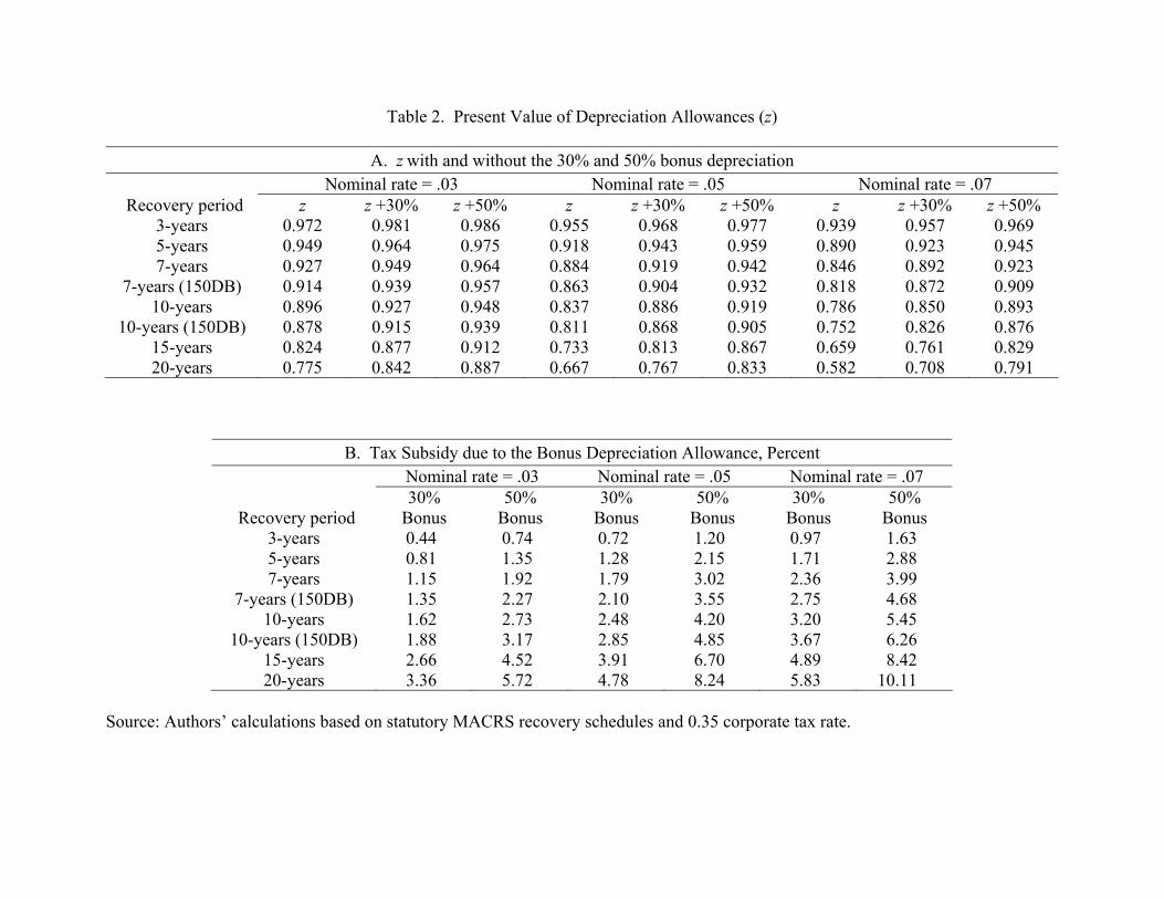
Table 2. Present Value of Depreciation Allowances (z)

A. z with and without the 30% and 50% bonus depreciation Nominal rate = .03 Nominal rate = .05 Nominal rate = .07

Recovery period z z +30% z +50% z z +30% z +50% z z +30% z +50% 3-years 0.972 0.981 0.986 0.955 0.968 0.977 0.939 0.957 0.969 5-years 0.949 0.964 0.975 0.918 0.943 0.959 0.890 0.923 0.945 7-years 0.927 0.949 0.964 0.884 0.919 0.942 0.846 0.892 0.923

7-years (150DB) 0.914 0.939 0.957 0.863 0.904 0.932 0.818 0.872 0.909 10-years 0.896 0.927 0.948 0.837 0.886 0.919 0.786 0.850 0.893

10-years (150DB) 0.878 0.915 0.939 0.811 0.868 0.905 0.752 0.826 0.876 15-years 0.824 0.877 0.912 0.733 0.813 0.867 0.659 0.761 0.829 20-years 0.775 0.842 0.887 0.667 0.767 0.833 0.582 0.708 0.791

B. Tax Subsidy due to the Bonus Depreciation Allowance, Percent Nominal rate = .03 Nominal rate = .05 Nominal rate = .07

Recovery period 30%

Bonus 50%

Bonus 30%

Bonus 50%

Bonus 30%

Bonus 50%

Bonus 3-years 0.44 0.74 0.72 1.20 0.97 1.63 5-years 0.81 1.35 1.28 2.15 1.71 2.88 7-years 1.15 1.92 1.79 3.02 2.36 3.99

7-years (150DB) 1.35 2.27 2.10 3.55 2.75 4.68 10-years 1.62 2.73 2.48 4.20 3.20 5.45

10-years (150DB) 1.88 3.17 2.85 4.85 3.67 6.26 15-years 2.66 4.52 3.91 6.70 4.89 8.42 20-years 3.36 5.72 4.78 8.24 5.83 10.11

Source: Authors’ calculations based on statutory MACRS recovery schedules and 0.35 corporate tax rate.

Table 3. Baseline Parameters

Parameter Baseline Value

Discount factor, annual rate (β ) 0.96

Capital share (α ) 0.38

Labor supply elasticity (η ) 0.5

Elasticity of intertemporal substitution of consumption (σ ) 0.2

Average Inflation Rate (π ) 0.03

Curvature of adjustment cost functions ( ξ ) 4

Elasticity of Capital Substitution (ρ ) 1

Tax Rate on Capital Earnings ( πτ ) 0.2235

Tax Rate on Earnings Distribution ( dτ ) 0.2975

Table 4. Annual Economic and Tax Depreciation Rates by Type of Capital

m Type of Capital

Economic Depreciation

mδ

Tax Depreciation

ˆmδ

Fraction of Investment (percent)

1 Construction equipment and tractors 0.17 0.40 1.38

2 Vehicles; office and computing equipment 0.30 0.40 28.49

3 Agricultural equipment 0.097 0.21 1.16

4 General equipment (incl. rail, furniture, aircraft, instruments, mining and oil, and household equipment) 0.100 0.29 21.66

5 Engines and turbines 0.079 0.10 0.40

6 Industrial buildings (incl. religious, education buildings, and hospitals) 0.03 0.03 11.60

7 Farm structures; rail; and electric power structures 0.025 0.08 2.02

8 Telephone, telegraph and misc. power and utility structures 0.04 0.10 1.62

9 Mining, shafts and wells 0.056 0.20 1.73

10 Residential and other structures 0.02 -- 28.46

Note: Authors’ calculations based on MACRS recovery schedules. For the calibration, these farm buildings do not include single purpose agricultural structures. Single purpose agricultural structures have a 10-year recovery period and are depreciated with a 150% DB method under MACRS. Farm structures other than single purpose structures are 20-year property (150% DB). In the data, farm structures are aggregated into one category. The last column gives fraction of investment since 1990 accounted for by the type. These types account for 98.5 of total investment. Excluded categories are water vessels, and lodging, recreation and amusement structures.

Table 5. Simulated Effects of a 30 Percent Bonus Depreciation Allowance: Alternative Parameters

Parameters GDP Employment

Change from Trend (percent)

Change (billions of dollars)

Change from Trend (percent)

Number (1000s)

Baseline 0.075 8.3 0.079 103

Low Adjustment Costs, ξ = 2 0.095 10.4 0.091 118

Estimated (GLS) Adj. Costs, ξ = 2.8 0.085 9.4 0.086 112

Full internal finance, τ d = 0 0.129 14.2 0.153 199

Internal finance with high profit tax, τ d = 0, τ π = 0.35 0.210 23.1 0.250 325

High Labor Supply Elasticity, η = 1 0.101 11.0 0.116 151

Log preferences (High IES), σ = 1 0.071 7.8 0.062 81

High nominal interest rates, π = 4 0.084 9.2 0.089 114

Low nominal interest rates, π = 2 0.066 7.2 0.070 91

Note: This table shows the results of simulating the effect of the 30% bonus depreciation provisions of Job Creation and Worker Assistance Act of 2002 (JCWAA) on 2003 GDP and employment. Parameters other than those specified in the table are set at their baseline values in Table 3.

Table 6. Economic and MACRS Depreciation by Detailed Type of Capital

Type of Capital Economic Depreciation

Rate mδ

Recovery Period

Depreciation Method

Tax Depreciation

Rate ˆmδ

Computers and peripheral equipment 0.300 5 200 0.400 Software 0.300 5 200 0.400 Communication equipment 0.300 5 200 0.400 Medical equipment and instruments 0.135 7 200 0.286 Nonmedical instruments 0.135 7 200 0.286 Photocopy and related equipment 0.180 5 200 0.400 Office and accounting equipment 0.150 5 200 0.400 Fabricated metal products 0.092 7 200 0.286 Steam engines 0.052 15 150 0.100 Internal combustion engines 0.210 15 150 0.100 Metalworking machinery 0.122 7 200 0.286 Special industry machinery 0.103 7 200 0.286 General industrial equipment 0.107 7 200 0.286 Electrical transmission and distribution, industrial apparatus 0.050 7 200 0.286 Trucks, buses, and truck trailers 0.190 5 200 0.400 Autos 0.165 5 200 0.400 Aircraft 0.110 7 200 0.286 Ships and boats 0.060 10 200 0.200 Railroad equipment 0.060 7 200 0.286 Farm tractors 0.145 5 150 0.300 Other agricultural machinery 0.118 7 150 0.214 Construction tractors 0.163 5 200 0.400 Other construction machinery 0.155 5 200 0.400 Mining and oilfield machinery 0.150 7 200 0.286 Service industry machinery 0.165 7 200 0.286 Commercial, including office buildings 0.025 39 SL 0.026 Hospitals and special care structures 0.019 39 SL 0.026 Manufacturing structures 0.031 39 SL 0.026 Electric structures 0.021 20 150 0.075 Other power structures 0.024 15 150 0.100 Communication structures 0.024 15 150 0.100 Petroleum and natural gas 0.075 5 SL 0.200 Mining 0.045 5 SL 0.200 Religious structures 0.019 39 SL 0.026 Educational structures 0.019 39 SL 0.026 Railroad structures 0.018 20 150 0.075 Farm structures 0.024 20 150 0.075 Single-family structures 0.015 --- --- ---

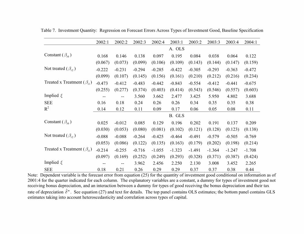
Table 7. Investment Quantity: Regression on Forecast Errors Across Types of Investment Good, Baseline Specification

2002:1 2002:2 2002:3 2002:4 2003:1 2003:2 2003:3 2003:4 2004:1 A. OLS Constant ( 0iβ ) 0.168 0.146 0.138 0.097 0.195 0.084 0.038 0.064 0.122 (0.067) (0.073) (0.099) (0.106) (0.109) (0.143) (0.144) (0.147) (0.159) Not treated ( 2iβ ) -0.222 -0.231 -0.294 -0.285 -0.422 -0.305 -0.293 -0.363 -0.472 (0.099) (0.107) (0.145) (0.156) (0.161) (0.210) (0.212) (0.216) (0.234) Treated x Treatment ( 1iβ ) -0.473 -0.412 -0.483 -0.442 -0.843 -0.554 -0.412 -0.441 -0.675 (0.255) (0.277) (0.374) (0.403) (0.414) (0.543) (0.546) (0.557) (0.603) Implied ξ -- -- 3.560 3.662 2.477 3.425 5.950 4.802 3.688 SEE 0.16 0.18 0.24 0.26 0.26 0.34 0.35 0.35 0.38 R2 0.14 0.12 0.11 0.09 0.17 0.06 0.05 0.08 0.11 B. GLS Constant ( 0iβ ) 0.025 -0.012 0.085 0.129 0.196 0.202 0.191 0.137 0.209 (0.030) (0.053) (0.080) (0.081) (0.102) (0.121) (0.128) (0.123) (0.138) Not treated ( 2iβ ) -0.088 -0.088 -0.264 -0.425 -0.464 -0.491 -0.579 -0.505 -0.769 (0.053) (0.086) (0.122) (0.135) (0.163) (0.179) (0.202) (0.198) (0.214) Treated x Treatment ( 1iβ ) -0.214 -0.255 -0.716 -1.055 -1.323 -1.491 -1.364 -1.247 -1.708 (0.097) (0.169) (0.252) (0.249) (0.293) (0.328) (0.371) (0.387) (0.424) Implied ξ -- -- 3.962 2.456 2.250 2.130 3.008 3.452 2.265 SEE 0.18 0.21 0.26 0.29 0.29 0.37 0.37 0.38 0.44

Note: Dependent variable is the forecast error from equation (25) for the quantity of investment good conditional on information as of 2001:4 for the quarter indicated for each column. The explanatory variables are a constant, a dummy for types of investment good not receiving bonus depreciation, and an interaction between a dummy for types of good receiving the bonus depreciation and their tax rate of depreciation ˆmδ . See equation (27) and text for details. The top panel contains OLS estimates; the bottom panel contains GLS estimates taking into account heteroscedasticity and correlation across types of capital.

Table 8. Investment Price: Regression on Forecast Errors Across Types of Investment Good, Baseline Specification

2002:1 2002:2 2002:3 2002:4 2003:1 2003:2 2003:3 2003:4 2004:1 A. OLS Constant ( 0iβ ) 0.002 0.005 0.009 0.002 0.006 0.003 -0.006 -0.018 -0.019 (0.004) (0.008) (0.013) (0.016) (0.017) (0.020) (0.023) (0.028) (0.032) Not treated ( 2iβ ) 0.009 0.005 0.000 0.008 0.008 0.009 0.017 0.037 0.045 (0.006) (0.012) (0.019) (0.024) (0.025) (0.029) (0.034) (0.041) (0.047) Treated x Treatment ( 1iβ ) -0.009 -0.032 -0.051 -0.026 -0.037 -0.032 0.009 0.063 0.060 (0.015) (0.031) (0.050) (0.061) (0.065) (0.075) (0.089) (0.106) (0.121) SEE 0.01 0.02 0.03 0.04 0.04 0.05 0.06 0.07 0.08 R2 0.15 0.08 0.05 0.02 0.03 0.02 0.01 0.02 0.03 B. GLS Constant ( 0iβ ) -0.001 -0.007 -0.002 -0.003 -0.005 -0.010 -0.024 -0.029 -0.021 (0.006) (0.008) (0.011) (0.011) (0.012) (0.014) (0.017) (0.019) (0.018) Not treated ( 2iβ ) 0.010 0.017 0.016 0.020 0.027 0.030 0.037 0.042 0.038 (0.002) (0.004) (0.005) (0.006) (0.007) (0.008) (0.009) (0.011) (0.011) Treated x Treatment ( 1iβ ) 0.042 0.083 0.070 0.086 0.096 0.128 0.195 0.196 0.208 (0.016) (0.024) (0.036) (0.037) (0.040) (0.050) (0.060) (0.063) (0.066) SEE 0.01 0.03 0.04 0.05 0.05 0.06 0.07 0.07 0.08

Note: Dependent variable is the forecast error from equation (26) for the relative price of investment good conditional on information as of 2001:4 for the quarter indicated for each column. The explanatory variables are a constant, a dummy for types of investment good not receiving bonus depreciation, and an interaction between a dummy for types of good receiving the bonus depreciation and their tax rate of depreciation ˆmδ . See equation (28) and text for details. The top panel contains OLS estimates; the bottom panel contains GLS estimates taking into account heteroscedasticity and correlation across types of capital.

Table A.1: MACRS Recovery Schedules by Recovery period, Percent per Year of Life Year 3-year 5-year 7-year 10-year 15-year 20-year 27½-year 39-year

1 33.33 20.00 14.29 10.00 5.00 3.750 1.970 1.390 2 44.45 32.00 24.49 18.00 9.50 7.219 3.636 2.564 3 14.81 19.20 17.49 14.40 8.55 6.677 3.636 2.564 4 7.41 11.52 12.49 11.52 7.70 6.177 3.636 2.564 5 11.52 8.93 9.22 6.93 5.713 3.636 2.564 6 5.76 8.92 7.37 6.23 5.285 3.636 2.564 7 8.93 6.55 5.90 4.888 3.636 2.564 8 4.46 6.55 5.90 4.522 3.636 2.564 9 6.56 5.91 4.462 3.636 2.564 10 6.55 5.90 4.461 3.636 2.564 11 3.28 5.91 4.462 3.636 2.564 12 5.90 4.461 3.636 2.564 13 5.91 4.462 3.636 2.564 14 5.90 4.461 3.636 2.564 15 5.91 4.462 3.636 2.564 16 2.95 4.461 3.636 2.564 17 4.462 3.636 2.564 18 4.461 3.636 2.564 19 4.462 3.636 2.564 20 4.461 3.636 2.564 21 2.231 3.636 2.564

22-27 3.636 2.564 28 3.485 2.564

29-39 2.564 40 0.963

Notes: 15 and 20-year property are recovered with a 150% declining balance method. The 27.5 and 39-year property classes are recovered with a straight-line method with a mid-month dating convention. Source: IRS Publication 946, How to Depreciate Property.

ϕ

Low ξ (elastic supply)

High ξ (inelastic supply)

1ϕ

0ϕ

tax subsidy ⎫⎪⎪⎬⎪⎪⎭

I1 | low I ξ 1 | high I ξ 0I

Figure 1: Price Reactions to Temporary Investment Subsidies.

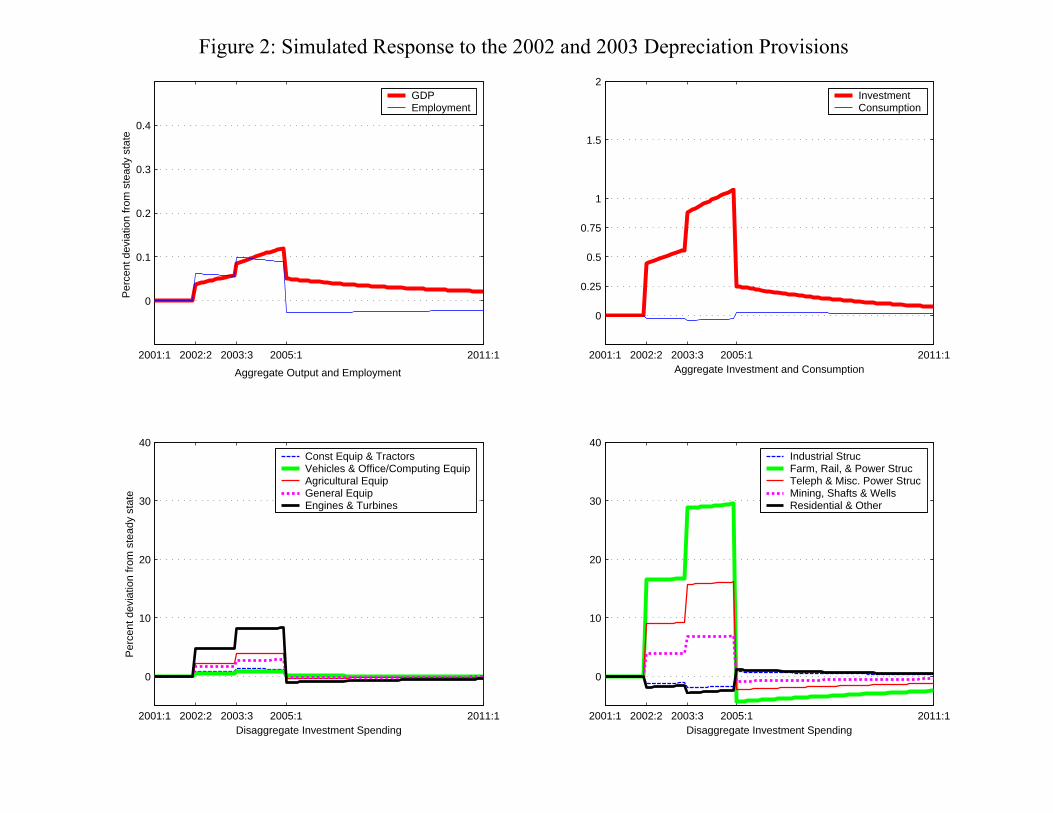
2001:1 2002:2 2003:3 2005:1 2011:1

0

10

20

30

40

Per

cent

dev

iatio

n fro

m s

tead

y st

ate

Disaggregate Investment Spending

Const Equip & TractorsVehicles & Office/Computing EquipAgricultural EquipGeneral EquipEngines & Turbines

2001:1 2002:2 2003:3 2005:1 2011:1

0

10

20

30

40

Disaggregate Investment Spending

Industrial StrucFarm, Rail, & Power StrucTeleph & Misc. Power StrucMining, Shafts & WellsResidential & Other

2001:1 2002:2 2003:3 2005:1 2011:1

0

0.1

0.2

0.3

0.4P

erce

nt d

evia

tion

from

ste

ady

stat

e

Aggregate Output and Employment

GDPEmployment

2001:1 2002:2 2003:3 2005:1 2011:1

0

0.25

0.5

0.75

1

1.5

2

Aggregate Investment and Consumption

InvestmentConsumption

Figure 2: Simulated Response to the 2002 and 2003 Depreciation Provisions

Figure 3: Simulated Changes in Investment and Relative Prices by Type of Capital

0 0.1 0.2 0.3 0.4 0.5

0

10

20

30

402002:4

Perc

ent D

evia

tion:

Rea

l Inv

estm

ent S

pend

ing

0 0.1 0.2 0.3 0.4 0.5

0

10

20

30

402004:1

0 0.1 0.2 0.3 0.4 0.5

0

1

2

3

4

Tax Depreciation Rate

Perc

ent D

evia

tion:

Rel

ativ

e Sh

adow

Pric

e

0 0.1 0.2 0.3 0.4 0.5

0

1

2

3

4

Tax Depreciation Rate

Note: Simulated response of investment and shadow prices for various types of capital to the 2002 and 2003 bonus depreciation policy as of 2002:4 and 2004:1. The tax depreciation rate ( ) is on the horizontal axis. Percent deviation from steady state is on the vertical axis. Circles are numerical calculations; diamonds are approximate calculations based on equations (22) and (24). Solid markers are for capital that qualifies for bonus depreciation. Empty markers are for capital that does not qualify.

ˆmδ

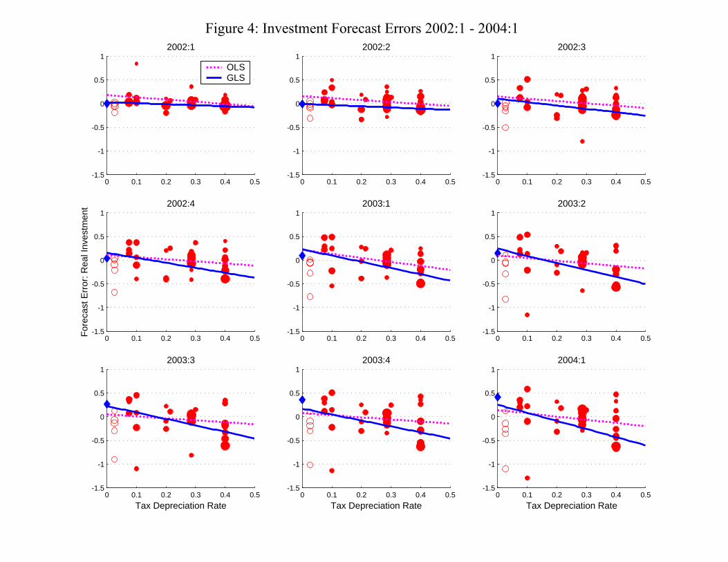
0 0.1 0.2 0.3 0.4 0.5-1.5

-1

-0.5

0

0.5

12002:1

OLSGLS

0 0.1 0.2 0.3 0.4 0.5-1.5

-1

-0.5

0

0.5

12002:2

0 0.1 0.2 0.3 0.4 0.5-1.5

-1

-0.5

0

0.5

12002:3

0 0.1 0.2 0.3 0.4 0.5-1.5

-1

-0.5

0

0.5

12002:4

Fore

cast

Err

or: R

eal I

nves

tmen

t

0 0.1 0.2 0.3 0.4 0.5-1.5

-1

-0.5

0

0.5

12003:1

0 0.1 0.2 0.3 0.4 0.5-1.5

-1

-0.5

0

0.5

12003:2

0 0.1 0.2 0.3 0.4 0.5-1.5

-1

-0.5

0

0.5

12003:3

Tax Depreciation Rate0 0.1 0.2 0.3 0.4 0.5

-1.5

-1

-0.5

0

0.5

12003:4

Tax Depreciation Rate0 0.1 0.2 0.3 0.4 0.5

-1.5

-1

-0.5

0

0.5

12004:1

Tax Depreciation Rate

Figure 4: Investment Forecast Errors 2002:1 - 2004:1

0 0.1 0.2 0.3 0.4 0.5-0.2

-0.1

0

0.1

0.2

0.3

0.4

0.52002:1

OLSGLS

0 0.1 0.2 0.3 0.4 0.5-0.2

-0.1

0

0.1

0.2

0.3

0.4

0.52002:2

0 0.1 0.2 0.3 0.4 0.5-0.2

-0.1

0

0.1

0.2

0.3

0.4

0.52002:3

0 0.1 0.2 0.3 0.4 0.5-0.2

-0.1

0

0.1

0.2

0.3

0.4

0.52002:4

Fore

cast

Err

or: R

eal R

elat

ive

Pric

es

0 0.1 0.2 0.3 0.4 0.5-0.2

-0.1

0

0.1

0.2

0.3

0.4

0.52003:1

0 0.1 0.2 0.3 0.4 0.5-0.2

-0.1

0

0.1

0.2

0.3

0.4

0.52003:2

0 0.1 0.2 0.3 0.4 0.5-0.2

-0.1

0

0.1

0.2

0.3

0.4

0.52003:3

Tax Depreciation Rate0 0.1 0.2 0.3 0.4 0.5

-0.2

-0.1

0

0.1

0.2

0.3

0.4

0.52003:4

Tax Depreciation Rate0 0.1 0.2 0.3 0.4 0.5

-0.2

-0.1

0

0.1

0.2

0.3

0.4

0.52004:1

Tax Depreciation Rate

Figure 5: Price Forecast Errors 2002:1 - 2004:1