In vivo study of optical speckle decorrelation time across ...biophot/publications/pdf/108-BiomedOptExp... · exposure speckle imaging,” Opt. Express 16(3), 1975–1989 (2008)

In vivo study of optical speckle decorrelation time across depths in the mouse brain

MUHAMMAD MOHSIN QURESHI,1,4 JOSHUA BRAKE,2,4 HEE-JAE JEON,1 HAOWEN RUAN,2 YAN LIU,2 ABDUL MOHAIMEN SAFI,1 TAE JOONG EOM,3 CHANGHUEI YANG,2 AND EUIHEON CHUNG

1,* 1Department of Biomedical Science and Engineering, Institute of Integrated Technology (IIT), Gwangju Institute of Science and Technology (GIST), 123 Cheomdangwagi-Ro, Buk-gu, Gwangju 61005, South Korea 2Department of Electrical Engineering, California Institute of Technology, Pasadena, California 91125, USA 3Advanced Photonics Research Institute, Gwangju Institute of Science and Technology (GIST), 123 Cheomdangwagi-Ro, Buk-gu, Gwangju 61005, South Korea 4Co-first authors with equal contribution *[email protected]

Abstract: The strong optical scattering of biological tissue confounds our ability to focus light deeply into the brain beyond depths of a few hundred microns. This challenge can be potentially overcome by exploiting wavefront shaping techniques which allow light to be focused through or inside scattering media. However, these techniques require the scattering medium to be static, as changes in the arrangement of the scatterers between the wavefront recording and playback steps reduce the fidelity of the focus that is formed. Furthermore, as the thickness of the scattering medium increases, the influence of the dynamic nature becomes more severe due to the growing number of scattering events experienced by each photon. In this paper, by examining the scattering dynamics in the mouse brain in vivo via multispeckle diffusing wave spectroscopy (MSDWS) using a custom fiber probe that simulates a point-like source within the brain, we investigate the relationship between this decorrelation time and the depth of the point-like light source inside the living mouse brain at depths up to 3.2 mm. © 2017 Optical Society of America

OCIS codes: (030.6140) Speckle; (170.3660) Light propagation in tissues; (170.7050) Turbid media.

References and links

1. J. Mertz, Introduction to Optical Microscopy (Roberts and Company, 2010). 2. V. Ntziachristos, “Going deeper than microscopy: the optical imaging frontier in biology,” Nat. Methods 7(8),

603–614 (2010). 3. L. V. Wang and W. Hsin-I, Biomedical Optics: Principles and Imaging (John Wiley & Sons, 2012). 4. S. L. Jacques, “Optical Properties of Biological Tissues: A Review,” Phys. Med. Biol. 58(11), R37–R61 (2013). 5. A. P. Mosk, A. Lagendijk, G. Lerosey, and M. Fink, “Controlling waves in space and time for imaging and

focusing in complex media,” Nat. Photonics 6, 283–292 (2012). 6. H. Yu, J. Park, K. Lee, J. Yoon, K. Kim, S. Lee, and Y. Park, “Recent advances in wavefront shaping techniques

for biomedical applications,” Curr. Appl. Phys. 15, 632–641 (2015). 7. R. Horstmeyer, H. Ruan, and C. Yang, “Guidestar-assisted wavefront-shaping methods for focusing light into

biological tissue,” Nat. Photonics 9, 563–571 (2015). 8. S. Rotter and S. Gigan, “Light fields in complex media: Mesoscopic scattering meets wave control,” Rev. Mod.

Phys. 89, 015005 (2017). 9. I. M. Vellekoop, “Feedback-based wavefront shaping,” Opt. Express 23(9), 12189–12206 (2015). 10. Z. Yaqoob, D. Psaltis, M. S. Feld, and C. Yang, “Optical phase conjugation for turbidity suppression in

biological samples,” Nat. Photonics 2(2), 110–115 (2008). 11. S. M. Popoff, G. Lerosey, R. Carminati, M. Fink, A. C. Boccara, and S. Gigan, “Measuring the Transmission

Matrix in Optics: An Approach to the Study and Control of Light Propagation in Disordered Media,” Phys. Rev. Lett. 104(10), 100601 (2010).

12. M. Jang, H. Ruan, I. M. Vellekoop, B. Judkewitz, E. Chung, and C. Yang, “Relation between speckle decorrelation and optical phase conjugation (OPC)-based turbidity suppression through dynamic scattering media: a study on in vivo mouse skin,” Biomed. Opt. Express 6(1), 72–85 (2014).

Vol. 8, No. 11 | 1 Nov 2017 | BIOMEDICAL OPTICS EXPRESS 4855

#304952 Journal © 2017

https://doi.org/10.1364/BOE.8.004855 Received 16 Aug 2017; revised 10 Sep 2017; accepted 25 Sep 2017; published 4 Oct 2017

https://crossmark.crossref.org/dialog/?doi=10.1364/BOE.8.004855&domain=pdf&date_stamp=2017-10-04

13. Y. Liu, P. Lai, C. Ma, X. Xu, A. A. Grabar, and L. V. Wang, “Optical focusing deep inside dynamic scattering media with near-infrared time-reversed ultrasonically encoded (TRUE) light,” Nat. Commun. 6, 5904 (2015).

14. I. M. Vellekoop, and A. P. Mosk, “Phase control algorithms for focusing light through turbid media,” Opt. Commun. 281, 3071–3080 (2008).

15. Y. Choi, T. D. Yang, C. Fang-Yen, P. Kang, K. J. Lee, R. R. Dasari, M. S. Feld, and W. Choi, “Overcoming the diffraction limit using multiple light scattering in a highly disordered medium,” Phys. Rev. Lett. 107(2), 023902 (2011).

16. D. Wang, E. H. Zhou, J. Brake, H. Ruan, M. Jang, and C. Yang, “Focusing through dynamic tissue with millisecond digital optical phase conjugation,” Optica 2(8), 728–735 (2015).

17. Y. Liu, C. Ma, Y. Shen, J. Shi, and L. V. Wang, “Focusing light inside dynamic scattering media with millisecond digital optical phase conjugation,” Optica 4(2), 280–288 (2017).

18. C. Ma, F. Zhou, Y. Liu, and L. V. Wang, “Single-exposure optical focusing inside scattering media using binarized time-reversed adapted perturbation,” Optica 2, 869–876 (2015).

19. D. Akbulut, T. J. Huisman, E. G. van Putten, W. L. Vos, and A. P. Mosk, “Focusing light through random photonic media by binary amplitude modulation,” Opt. Express 19(5), 4017–4029 (2011).

20. D. B. Conkey, A. M. Caravaca-Aguirre, and R. Piestun, “High-speed scattering medium characterization with application to focusing light through turbid media,” Opt. Express 20(2), 1733–1740 (2012).

21. M. Cui and C. Yang, “Implementation of a digital optical phase conjugation system and its application to study the robustness of turbidity suppression by phase conjugation,” Opt. Express 18(4), 3444–3455 (2010).

22. J. Brake, M. Jang, and C. Yang, “Analyzing the relationship between decorrelation time and tissue thickness in acute rat brain slices using multispeckle diffusing wave spectroscopy,” J. Opt. Soc. Am. A 33(2), 270–275 (2016).

23. S. Sun, B. R. Hayes-Gill, D. He, Y. Zhu, and S. P. Morgan, “Multi-exposure laser speckle contrast imaging using a high frame rate CMOS sensor with a field programmable gate array,” Opt. Lett. 40(20), 4587–4590 (2015).

24. H. Ruan, M. L. Mather, and S. P. Morgan, “Pulse inversion ultrasound modulated optical tomography,” Opt. Lett. 37(10), 1658–1660 (2012).

25. D. J. Pine, D. A. Weitz, P. M. Chaikin, and E. Herbolzheimer, “Diffusing wave spectroscopy,” Phys. Rev. Lett. 60(12), 1134–1137 (1988).

26. G. Maret and P. E. Wolf, “Multiple light scattering from disordered media. The effect of brownian motion of scatterers,” Z. Phys. B Condens. Matter 65, 409–413 (1987).

27. F. C. MacKintosh and S. John, “Diffusing-wave spectroscopy and multiple scattering of light in correlated random media,” Phys. Rev. B Condens. Matter 40(4), 2383–2406 (1989).

28. A. B. Parthasarathy, W. J. Tom, A. Gopal, X. Zhang, and A. K. Dunn, “Robust flow measurement with multi-exposure speckle imaging,” Opt. Express 16(3), 1975–1989 (2008).

29. P.-A. Lemieux and D. J. Durian, “Investigating non-Gaussian scattering processes by using nth-order intensity correlation functions,” J. Opt. Soc. Am. A 16, 1651 (1999).

30. M. Medebach, N. Freiberger, and O. Glatter, “Dynamic light scattering in turbid nonergodic media,” Rev. Sci. Instrum. 79(7), 073907 (2008).

31. V. Viasnoff, F. Lequeux, and D. J. Pine, “Multispeckle diffusing-wave spectroscopy: A tool to study slow relaxation and time-dependent dynamics,” Rev. Sci. Instrum. 73, 2336–2344 (2002).

32. J. W. Goodman, “Some fundamental properties of speckle,” J. Opt. Soc. Am. 66, 1145–1150 (1976). 33. R. Mostany and C. Portera-Cailliau, “A craniotomy surgery procedure for chronic brain imaging,” J. Vis. Exp.

12, 680 (2008). 34. A. Cho, C. Yeon, D. Kim, and E. Chung, “Laser speckle contrast imaging for measuring cerebral blood flow

changes caused by electrical sensory stimulation,” J. Opt. Soc. Korea 20, 88–93 (2016). 35. D. Kobat, N. G. Horton, and C. Xu, “In vivo two-photon microscopy to 1.6-mm depth in mouse cortex,” J.

Biomed. Opt. 16(10), 106014 (2011). 36. D. G. Ouzounov, T. Wang, M. Wang, D. D. Feng, N. G. Horton, J. C. Cruz-Hernández, Y.-T. Cheng, J. Reimer,

A. S. Tolias, N. Nishimura, and C. Xu, “In vivo three-photon imaging of activity of GCaMP6-labeled neurons deep in intact mouse brain,” Nat. Methods 14(4), 388–390 (2017).

37. J. Li, G. Ku, and L. V. Wang, “Ultrasound-modulated optical tomography of biological tissue by use of contrast of laser speckles,” Appl. Opt. 41(28), 6030–6035 (2002).

38. L. Tian, S. A. Hires, T. Mao, D. Huber, M. E. Chiappe, S. H. Chalasani, L. Petreanu, J. Akerboom, S. A. McKinney, E. R. Schreiter, C. I. Bargmann, V. Jayaraman, K. Svoboda, and L. L. Looger, “Imaging neural activity in worms, flies and mice with improved GCaMP calcium indicators,” Nat. Methods 6(12), 875–881 (2009).

39. K. Deisseroth, “Optogenetics,” Nat. Methods 8(1), 26–29 (2011). 40. T. Laforest, A. Verdant, A. Dupret, S. Gigan, F. Ramaz, and G. Tessier, “Monolithic device for on-chip fast

optical phase conjugation integrating an image sensor and a spatial light modulator,” Proc. SPIE - Int. Soc. Opt. Eng. 9022, 90220N (2014).

41. T. Laforest, A. Dupret, A. Verdant, F. Ramaz, S. Gigan, G. Tessier, and E. B. A. La Guillaume, “A 4000 Hz CMOS image sensor with in-pixel processing for light measurement and modulation,” 2013 IEEE 11th Int. New Circuits Syst. Conf. NEWCAS 2013 1–4 (2013).

42. I. N. Papadopoulos, J.-S. Jouhanneau, J. F. A. Poulet, and B. Judkewitz, “Scattering compensation by focus


scanning holographic aberration probing (F-SHARP),” Nat. Photonics 11, 116–123 (2016). 43. M. Kadobianskyi, I. N. Papadopoulos, T. Chaigne, R. Horstmeyer, and B. Judkewitz, “Scattering correlations of

time-gated light,” arXiv Prepr. 1–12 (2017).

1. Introduction

The use of light in biomedicine for imaging and therapeutic applications is powerful due to the ability to image and deliver light with high spatial resolution in a noninvasive and nondestructive manner. The wide array of light-matter interactions such as scattering, absorption, fluorescence, and Raman scattering offer many different contrast mechanisms that can be used to interrogate and understand biological processes [1]. However, the strong scattering nature of biological tissue in the optical regime limits conventional high-resolution imaging and light focusing techniques to superficial layers of several hundred microns or less [2].

For many years in optics, the scattering of light was assumed to be the fundamental limit for high-resolution light delivery deep into turbid media. However, recent work in the field of wavefront shaping has shown that light can be focused at depths beyond several transport mean free paths by appropriately shaping the input light field. This opens a new regime for optical focusing between the transport mean free path and the absorption limit which is typically two orders of magnitude larger [3, 4]. Focusing light to a targeted location inside or through scattering media with the aid of wavefront shaping works by finding an appropriate input light field pattern such that the light can constructively interfere at the desired locations. Since this demonstration, wavefront shaping methods have been an active area of research [5–8], and several approaches have been developed, including those based on feedback [9], phase conjugation [10], and transmission matrix measurement [11].

The initial wavefront shaping demonstrations used static scattering media such as white paint layers, opal diffusers, or fixed tissue. In these static samples, the scatterers within are often stable for periods of time ranging from minutes to hours, and therefore the optimal wavefront for forming constructive interference also remains constant over these time scales. However, many of the exciting applications for wavefront shaping are in living tissues where the optimal wavefront to focus light to a desired location varies with time due to Brownian motion and physiological motion such as breathing, heartbeat, and blood flow. While previous studies have demonstrated the ability to focus light through living tissue such as the mouse dorsal skin flap [12] or ear [13], the scattering of light by the vasculature in the brain significantly decreases the decorrelation time and prevents these methods from being translated directly for use in brain tissue in vivo.

Wavefront shaping systems are limited by both their wavefront measurement and playback schemes. Since the decorrelation time impacts system performance regardless of whether a feedback [14], transmission matrix [11, 15], or optical phase conjugation (OPC) [10, 12, 16, 17] based wavefront measurement scheme is used, it is a widely useful parameter for wavefront shaping systems. The decorrelation time is also helpful for evaluating wavefront playback schemes. These approaches have response times ranging from several tens of microseconds to several tens of milliseconds depending on whether nematic liquid crystal [12, 18], ferroelectric liquid crystal [17], or microelectromechanical systems based spatial light modulator (SLM) technologies are used [16, 19, 20]. Put together, the combined wavefront measurement and playback operation must take place within the decorrelation time to successfully focus light using wavefront shaping. This makes the synergistic combination of an appropriate measurement and playback scheme critical. Understanding the decorrelation time and its relationship to the tissue thickness is an important, widely applicable parameter of interest for designing new wavefront shaping systems to focus light beyond several transport mean free paths deep in tissue, especially for systems geared toward in vivo applications.

The time scale at which the wavefront varies can be measured by observing the speed at which it loses correlation with a previous copy of itself over time. This is typically


accomplished by computing a measure of the correlation between the wavefronts or speckle intensity patterns. Then, by fitting the correlation function, a figure of merit called the decorrelation time (or speckle correlation time) can be determined. The decorrelation time is defined as the time it takes for the correlation between the initial wavefront and the subsequently captured wavefronts to drop below a specific value. Previous studies [12, 13, 17, 21] have established the direct relationship between the speckle decorrelation time and the fidelity of the wavefront reconstruction for delivering light into a focus, and also characterized the speckle decorrelation times associated with living ear tissue both with and without the contribution of blood flow. More recently, the relationship between decorrelation time and tissue thickness was studied in acute rat brain slices [22]. However, up until now, the decorrelation time in the in vivo rodent brain and its relationship to the thickness of the tissue through which the light passes has not been directly measured or quantified.

In this study, we experimentally measure and report the relationship between the speckle decorrelation time and the depth of a point-like source inside the in vivo mouse brain. The results of this study provide an important order of magnitude measurement of the decorrelation time at a depth up to several millimeters below the surface of the brain. The experimental results included in this paper will help inform the development of wavefront shaping systems for in vivo applications such as deep tissue light focusing, imaging, and therapy and provide information for applying other optical techniques using speckle such as laser speckle contrast imaging (LSCI) [23] and ultrasound modulated optical tomography (UOT) [24] in the brain in vivo.

2. Theory

To measure the decorrelation time, we used the framework of diffusing wave spectroscopy (DWS) [25–27]. DWS is a technique that uses measured fluctuations in the scattered optical field passing through a dynamic scattering medium to determine the characteristic time scale associated with the movement of the scatterers within the medium. The key quantity of interest in DWS is the temporal autocorrelation function of the electric field, ( )1g τ , which

can be directly derived from the interfering contributions of photons of varying path lengths. Due to the multiple scattering process, the path length fluctuations reflect the movement of the scatterers. These fluctuations impact the decay time of the autocorrelation function, allowing the decay time of the autocorrelation function to be used to measure the movement of the scatterers inside the medium.

The field autocorrelation function ( )1g τ is difficult to measure directly due to the

limitation of intensity-only detectors such as photodiodes and conventional CMOS and CCD cameras. Therefore, the intensity autocorrelation function ( )2g τ is typically recorded instead

of ( )1g τ since it can be directly measured with intensity-only detectors. Then, using the

appropriate version of the Siegert relation, the intensity autocorrelation function can be used to relate the intensity and field autocorrelation functions [25, 26, 28, 29]. While the exact relationship between the dynamics of the scatterers and ( )2g τ must be retrieved by using the

appropriate Siegert relation, the decay time of ( )2g τ itself is a helpful metric to establish the

decay time of the measured optical wavefront. In the first experimental demonstrations, DWS was implemented by measuring the

temporal evolution of a single speckle grain to compute the autocorrelation function [25,26]. This required long measurement times and that the sample be ergodic [30]. One method to address these challenges is to measure many speckles in parallel using an array detector such as a digital camera in lieu of a single speckle on a photodiode. This configuration, called multispeckle diffusing wave spectroscopy (MSDWS), enables many speckles to be measured in parallel which reduces the necessary measurement time, and thus the requirement for


ergodicity since each group of pixels corresponding to a single speckle can be considered a separate temporal measurement [31]. While the time scales that can be probed are slower than those accessible with photon counting devices such as photo multiplier tubes or avalanche photodiodes, state of the art sCMOS cameras can achieve sub-millisecond resolution and therefore are advantageous when the autocorrelation function decays on the order of a few milliseconds.

To calculate the autocorrelation function, a series of intensity measurements are made. In the case of MSDWS, these are camera speckle images. Then, using this temporal series of images, the autocorrelation function ( )2g τ is calculated by computing the correlation

function between the sample frame at delay time τ and the initial frame in the series taken at time 0t .This calculation is described by

( ) ( ) ( )( ) ( )

0 02

0 0

I t I tg

I t I t

ττ

τ ⋅ +

= +

(1)

where I is the intensity image captured on the sensor, τ is the delay time after the original frame measured at 0t , and ⋅ ⋅ ⋅ represents an average over the elements of the element-wise

multiplication of the frames. For a fully developed speckle pattern with an exponential intensity distribution [32], ( )2g τ theoretically decays from a value of 2 (completely

correlated) to a value of 1 (no correlation). However, partially developed speckle or experimental noise (e.g. due to blurring of the speckle pattern within the exposure time) means that in practice ( )2g τ typically decays from a value less than 2 to a steady state value

greater than 1. By fitting this curve with an appropriate model based on the experimental configuration, the decorrelation time can be determined.

3. Experimental setup

The experimental setup is shown in Fig. 1. A Helium-neon (HeNe) laser with a wavelength of λ = 632.8 nm and an output power of 17 mW (Research Electro-Optics Inc., Colorado, USA) was used to illuminate the brain through a custom optical fiber probe embedded into the brain. A microscope objective lens (RMS4X, NA 0.10, Olympus) focused on the top surface of the brain was used along with a tube lens (180 mm) to image the speckle pattern onto an sCMOS camera (Neo 5.5 sCMOS, Andor Technology Ltd., Belfast, UK). A linear polarizer, placed in the infinity space between the microscope objective and tube lens, helped to improve the contrast of the captured speckle image. Camera frames were captured at the minimum exposure time of 0.103 ms which enabled a frame rate of 9701 fps.

To move the point-like source inside the brain, we used a mechanical micromanipulator (MN-153 Narishige, Japan) configured to move diagonally at a 45° angle with respect to the normal direction as shown in Fig. 1. The penetration depth d was calculated using the insertion angle (45°) and the translation distance s along the axis of the needle. Since the location of the fiber probe translated along the x-axis as well as along the z-axis as the micro manipulator was advanced, a sub-region (256 × 12 pixels, pixel size 6.5 µm) for each depth, centered at the maximum intensity of the diffuse light profile on the brain surface, was selected out of the full size frame (1200 × 12 pixels) to allow for consistent sampling of the speckle pattern directly above the fiber tip across depths. We also made sure to avoid large blood vessels near the pial surface of the brain when selecting the regions of interest for analysis as shown in Fig. 2(c). The iris size in the optical train was selected so the speckle size on the camera was ~2.2 × 2.2 pixels to satisfy the Nyquist criteria for sampling the speckle. The laser beam was coupled into a 105 μm core diameter (with jacket diameter 250 µm) multimode fiber (Thorlabs FG105LCA) and the other end of fiber tip inserted through a 26-gauge needle (inner diameter = 260 μm).


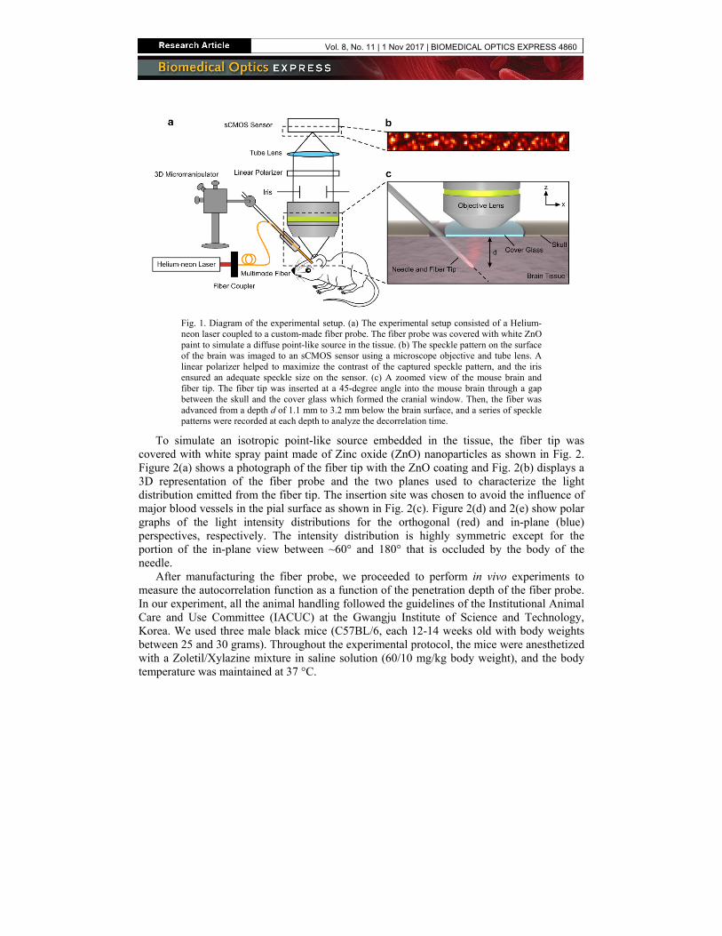
Fig. 1. Diagram of the experimental setup. (a) The experimental setup consisted of a Helium-neon laser coupled to a custom-made fiber probe. The fiber probe was covered with white ZnO paint to simulate a diffuse point-like source in the tissue. (b) The speckle pattern on the surface of the brain was imaged to an sCMOS sensor using a microscope objective and tube lens. A linear polarizer helped to maximize the contrast of the captured speckle pattern, and the iris ensured an adequate speckle size on the sensor. (c) A zoomed view of the mouse brain and fiber tip. The fiber tip was inserted at a 45-degree angle into the mouse brain through a gap between the skull and the cover glass which formed the cranial window. Then, the fiber was advanced from a depth d of 1.1 mm to 3.2 mm below the brain surface, and a series of speckle patterns were recorded at each depth to analyze the decorrelation time.

To simulate an isotropic point-like source embedded in the tissue, the fiber tip was covered with white spray paint made of Zinc oxide (ZnO) nanoparticles as shown in Fig. 2. Figure 2(a) shows a photograph of the fiber tip with the ZnO coating and Fig. 2(b) displays a 3D representation of the fiber probe and the two planes used to characterize the light distribution emitted from the fiber tip. The insertion site was chosen to avoid the influence of major blood vessels in the pial surface as shown in Fig. 2(c). Figure 2(d) and 2(e) show polar graphs of the light intensity distributions for the orthogonal (red) and in-plane (blue) perspectives, respectively. The intensity distribution is highly symmetric except for the portion of the in-plane view between ~60° and 180° that is occluded by the body of the needle.

After manufacturing the fiber probe, we proceeded to perform in vivo experiments to measure the autocorrelation function as a function of the penetration depth of the fiber probe. In our experiment, all the animal handling followed the guidelines of the Institutional Animal Care and Use Committee (IACUC) at the Gwangju Institute of Science and Technology, Korea. We used three male black mice (C57BL/6, each 12-14 weeks old with body weights between 25 and 30 grams). Throughout the experimental protocol, the mice were anesthetized with a Zoletil/Xylazine mixture in saline solution (60/10 mg/kg body weight), and the body temperature was maintained at 37 °C.


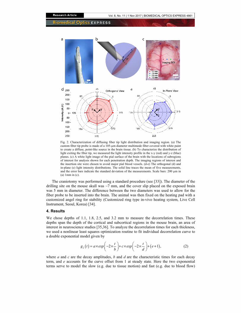
Fig. 2. Characterization of diffusing fiber tip light distribution and imaging region. (a) The custom fiber tip probe is made of a 105-µm diameter multimode fiber covered with white paint to create a diffuse, point-like source in the brain tissue. (b) To characterize the distribution of light exiting the fiber tip, we measured the light intensity profile in the x-y (red) and y-z (blue) planes. (c) A white light image of the pial surface of the brain with the locations of subregions of interest for analysis shown for each penetration depth. The imaging regions of interest and the insertion site were chosen to avoid major pial blood vessels. (d-e) The orthogonal (d) and in-plane (e) light intensity distributions. The solid line traces the mean of five measurements, and the error bars indicate the standard deviation of the measurements. Scale bars: 200 µm in (a) 1mm in (c).

The craniotomy was performed using a standard procedure (see [33]). The diameter of the drilling site on the mouse skull was ~7 mm, and the cover slip placed on the exposed brain was 5 mm in diameter. The difference between the two diameters was used to allow for the fiber probe to be inserted into the brain. The animal was then fixed on the heating pad with a customized angel ring for stability (Customized ring type in-vivo heating system, Live Cell Instrument, Seoul, Korea) [34].

4. Results

We chose depths of 1.1, 1.8, 2.5, and 3.2 mm to measure the decorrelation times. These depths span the depth of the cortical and subcortical regions in the mouse brain, an area of interest in neuroscience studies [35,36]. To analyze the decorrelation times for each thickness, we used a nonlinear least squares optimization routine to fit individual decorrelation curve to a double exponential model given by

( ) ( )2 2 2 1 ,t t

g t a exp c exp eb d

= × − × + × − × + +

(2)

where a and c are the decay amplitudes, b and d are the characteristic times for each decay term, and e accounts for the curve offset from 1 at steady state. Here the two exponential terms serve to model the slow (e.g. due to tissue motion) and fast (e.g. due to blood flow)


decorrelation time components. Then, the overall decorrelation time is determined by finding the time where the curve decay amplitude (a + c) decays to 1/e of its initial value.

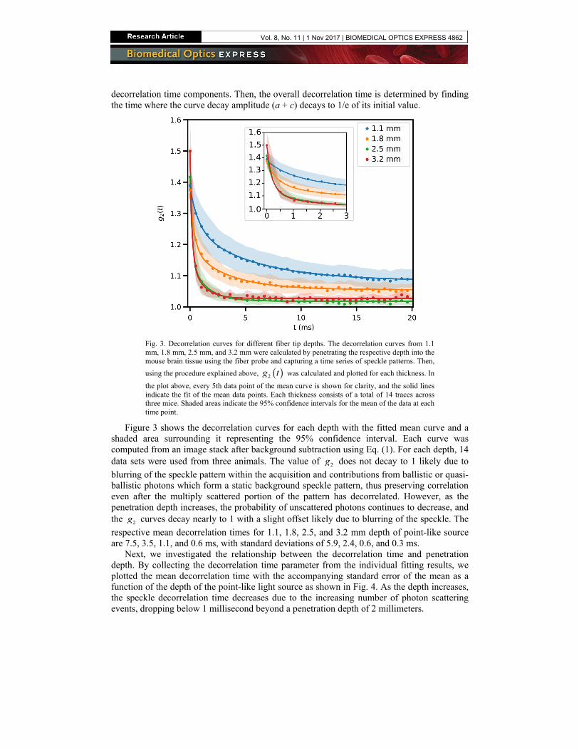
Fig. 3. Decorrelation curves for different fiber tip depths. The decorrelation curves from 1.1 mm, 1.8 mm, 2.5 mm, and 3.2 mm were calculated by penetrating the respective depth into the mouse brain tissue using the fiber probe and capturing a time series of speckle patterns. Then,

using the procedure explained above, ( )2g t was calculated and plotted for each thickness. In

the plot above, every 5th data point of the mean curve is shown for clarity, and the solid lines indicate the fit of the mean data points. Each thickness consists of a total of 14 traces across three mice. Shaded areas indicate the 95% confidence intervals for the mean of the data at each time point.

Figure 3 shows the decorrelation curves for each depth with the fitted mean curve and a shaded area surrounding it representing the 95% confidence interval. Each curve was computed from an image stack after background subtraction using Eq. (1). For each depth, 14 data sets were used from three animals. The value of 2g does not decay to 1 likely due to

blurring of the speckle pattern within the acquisition and contributions from ballistic or quasi-ballistic photons which form a static background speckle pattern, thus preserving correlation even after the multiply scattered portion of the pattern has decorrelated. However, as the penetration depth increases, the probability of unscattered photons continues to decrease, and the 2g curves decay nearly to 1 with a slight offset likely due to blurring of the speckle. The

respective mean decorrelation times for 1.1, 1.8, 2.5, and 3.2 mm depth of point-like source are 7.5, 3.5, 1.1, and 0.6 ms, with standard deviations of 5.9, 2.4, 0.6, and 0.3 ms.

Next, we investigated the relationship between the decorrelation time and penetration depth. By collecting the decorrelation time parameter from the individual fitting results, we plotted the mean decorrelation time with the accompanying standard error of the mean as a function of the depth of the point-like light source as shown in Fig. 4. As the depth increases, the speckle decorrelation time decreases due to the increasing number of photon scattering events, dropping below 1 millisecond beyond a penetration depth of 2 millimeters.


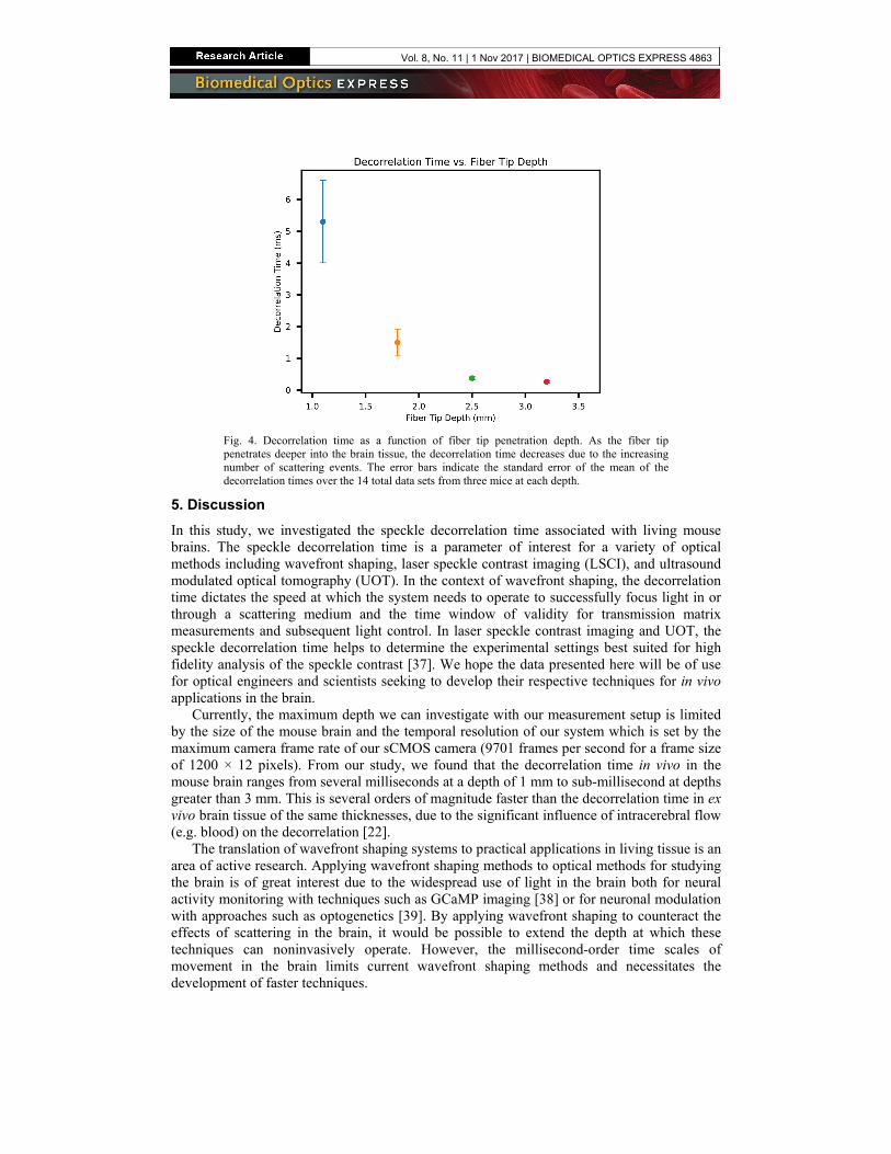
Fig. 4. Decorrelation time as a function of fiber tip penetration depth. As the fiber tip penetrates deeper into the brain tissue, the decorrelation time decreases due to the increasing number of scattering events. The error bars indicate the standard error of the mean of the decorrelation times over the 14 total data sets from three mice at each depth.

5. Discussion

In this study, we investigated the speckle decorrelation time associated with living mouse brains. The speckle decorrelation time is a parameter of interest for a variety of optical methods including wavefront shaping, laser speckle contrast imaging (LSCI), and ultrasound modulated optical tomography (UOT). In the context of wavefront shaping, the decorrelation time dictates the speed at which the system needs to operate to successfully focus light in or through a scattering medium and the time window of validity for transmission matrix measurements and subsequent light control. In laser speckle contrast imaging and UOT, the speckle decorrelation time helps to determine the experimental settings best suited for high fidelity analysis of the speckle contrast [37]. We hope the data presented here will be of use for optical engineers and scientists seeking to develop their respective techniques for in vivo applications in the brain.

Currently, the maximum depth we can investigate with our measurement setup is limited by the size of the mouse brain and the temporal resolution of our system which is set by the maximum camera frame rate of our sCMOS camera (9701 frames per second for a frame size of 1200 × 12 pixels). From our study, we found that the decorrelation time in vivo in the mouse brain ranges from several milliseconds at a depth of 1 mm to sub-millisecond at depths greater than 3 mm. This is several orders of magnitude faster than the decorrelation time in ex vivo brain tissue of the same thicknesses, due to the significant influence of intracerebral flow (e.g. blood) on the decorrelation [22].

The translation of wavefront shaping systems to practical applications in living tissue is an area of active research. Applying wavefront shaping methods to optical methods for studying the brain is of great interest due to the widespread use of light in the brain both for neural activity monitoring with techniques such as GCaMP imaging [38] or for neuronal modulation with approaches such as optogenetics [39]. By applying wavefront shaping to counteract the effects of scattering in the brain, it would be possible to extend the depth at which these techniques can noninvasively operate. However, the millisecond-order time scales of movement in the brain limits current wavefront shaping methods and necessitates the development of faster techniques.


Based on the decorrelation times measured in the in vivo mouse brain, this means that the maximum depth accessible with current wavefront shaping technology (minimum system latency of ~3 ms [17]) in the in vivo mouse brain is between 1 and 2 mm. Therefore, to develop wavefront shaping methods which are practical and robust for in vivo light focusing for applications such as high-resolution deep tissue optical imaging, noninvasive deep tissue optogenetics, and photodynamic therapy at depths several millimeters below the tissue surface, it will be necessary to develop faster wavefront shaping tools. We believe that one promising solution to this problem is the development of an integrated wavefront measurement and shaping device which combines SLM and camera pixels into a single unit [40,41]. This will allow for wavefront measurement and playback to be achieved on a parallel, per pixel basis thus enabling sub-millisecond focusing times which will increase the penetration depth of wavefront shaping techniques to several millimeters in vivo in the brain. Other strategies to increase the decorrelation time are to move to longer wavelengths in the near infrared regime where scattering is less severe or to use coherence gating and short pulses to extend the decorrelation time by selecting only minimally scattered photons [42,43].

In future experiments, we hope to investigate the decorrelation time of the living brain at longer, near-infrared wavelengths (900-1200 nm) since these may be of future interest for wavefront shaping applications. In addition, it would be interesting to compare the decorrelation time in awake, head-fixed mice compared to the decorrelation time measurements from the anesthetized mice used in this study. To analyze deeper penetration depths, we can also modify the system to use a point based detector with a faster temporal response than the sCMOS camera used in this study to record the dynamics of faster decorrelation processes.

In conclusion, we have shown for the first time the decorrelation time in the in vivo mouse brain up to 3.2 mm deep inside the mouse brain using a custom point-like fiber probe source. To take full advantage of our developed system, we have introduced a simple craniotomy to embed our point source at the desired angle in a minimally invasive manner to enable stable imaging over the course of the experiment. The results of this study will help to inform the development of future wavefront shaping systems for in vivo applications in the brain.

Funding

This work was supported in part by GIST Research Institute (GRI), and the GIST-Caltech Research Collaboration Project through a grant provided by GIST in 2017, a research grant (NRF-2016R1A2B4015381), the Brain Research Program (NRF-2017M3C7A 1044964) of the National Research Foundation (NRF), the KBRI basic research program through Korea Brain Research Institute (17-BR-04) funded by the Ministry of Science, ICT, Future Planning, the industrial convergence foundation construction program (N0002310) funded by the Ministry of Trade, Industry & Energy, and the National Institutes of Health (NIH) (U01NS090577). J.B. was supported by the National Institute of Biomedical Imaging, and Bioengineering (F31EB021153) under a Ruth L. Kirschstein National Research Service Award and by the Donna and Benjamin M. Rosen Bioengineering Center.

Acknowledgment

The authors thank Ms. Ji Hye Yang from GIST for her help during the animal experiment.

Disclosures

The authors declare that there are no conflicts of interest related to this article.


Documents

In vivo study of optical speckle decorrelation time across ...biophot/publications/pdf/108-BiomedOptExp... · exposure speckle imaging,” Opt. Express 16(3), 1975–1989 (2008)