Impact of Scene Decorrelation on Geosynchronous SAR … · Impact of Scene Decorrelation on Geosynchronous SAR Data ... We then assume the Billingsley Intrinsic Clutter Motion model,

IEEE TRANSACTIONS ON GEOSCIENCE AND REMOTE SENSING, VOL. 54, NO. 3, MARCH 2016 1635

Impact of Scene Decorrelation on GeosynchronousSAR Data Focusing

Andrea Recchia, Andrea Monti Guarnieri, Member, IEEE, Antoni Broquetas, Member, IEEE, and Antonio Leanza

Abstract—We discuss the effects of the clutter on geosynchro-nous SAR systems exploiting long integration times (from minutesto hours) to counteract for two-way propagation losses and in-crease azimuth resolution. Only stable targets will be correctlyfocused whereas unstable targets will spread their energy alongazimuth direction. We derive here a generic model for the spread-ing of the clutter energy based on the power spectral density ofthe clutter itself. We then assume the Billingsley Intrinsic ClutterMotion model, representing the clutter power spectrum as anexponential decay, and derive the expected GEOSAR signal-to-clutter ratio. We also provide some results from a Ground BasedRADAR experiment aimed at assessing the long-term clutter sta-tistics for different scenarios to complement the Internal ClutterMotion model, mainly derived for windblown trees. Finally, wediscuss the expected performances of two GEOSAR systems withdifferent acquisition geometries.

Index Terms—Focusing, Geosynchronous Synthetic ApertureRadar (GEOSAR), scene decorrelation, wind-blown clutter.

I. INTRODUCTION

A SYNTHETIC aperture radar (SAR) placed in geosyn-chronous orbit (GEOSAR) was first proposed at the end

of the 1970s [1], [2]. Since then, several GEOSAR systems havebeen proposed but never implemented due to both technologicalconstraints [3] and the presence of decorrelation sources im-pacting on the quality of the focused images [4]. Nevertheless,the growing interest in GEOSAR systems is justified by theirpotential applications. In particular, the daily revisit couldenable the near real time monitoring of geophysical phenomenawith time scales much faster than those currently observed withLow Earth Orbit SAR (LEOSAR) constellations.

GEOSAR systems exploit long integration times to increaseresolution and compensate spread losses, making the sceneresponse during the dwell time nonstable. From one side theAtmospheric Phase Screen (APS), if not properly compensated,could prevent data focusing when integration time extends fromseveral minutes to hours [5]–[7]. On the other hand the responseof the targets itself can change during the dwell time. Theenergy of nonstable targets, after focusing, will spread along

Manuscript received October 22, 2014; revised March 18, 2015 and July 17,2015; accepted August 14, 2015. Date of publication October 30, 2015; date ofcurrent version February 24, 2016.

A. Recchia, A. Monti Guarnieri, and A. Leanza are with the Dipartimentodi Elettronica, Informazione e Bioingegneria, Politecnico di Milano, 20133Milano, Italy (e-mail: [email protected]).

A. Broquetas is with Universitat Politecnica de Catalunya, 08034 Barcelona,Spain.

Color versions of one or more of the figures in this paper are available onlineat http://ieeexplore.ieee.org.

Digital Object Identifier 10.1109/TGRS.2015.2486385

azimuth direction affecting the signal-to-clutter ratio (SCR)even for very stable targets such as urban and rocky areas [4].

In the present paper we neglect atmospheric effects andconcentrate on the impact of the clutter decorrelation on aGEOSAR system. For short integration time SAR systems(< 1 s) the clutter is assumed stationary within the dwell timeand, after focusing, impairs the detection of the targets ofinterest. Unlike thermal noise, the SCR cannot be improved byincreasing the transmitted power but only enhancing the systemresolution. Ulaby and Dobson experimentally derived modelsfor the characterization of the clutter in terms of normalizedradar cross section (σ0) for different classes of terrain atdifferent grazing angles [8].

The increase of the integration time and the reduction ofthe wavelength in modern SAR systems, aimed at improvingresolution like in Spotlight SAR [9], pose the problem of non-stationary clutter, which also affects applications like movingtarget indication [10], [11]. For this reason, nonstationary clut-ter has been widely investigated by Billingsley, who introducedthe Internal Clutter Motion (ICM) model, experimentally de-rived for windblown trees at different bands (from L to X) [12].The ICM model is a good approximation of the nonstationaryclutter spectrum for observation times up to 1 min. The validityof the ICM model has never been proven for longer observationtimes like those exploited by a GEOSAR system, which canextend to hours [13], [14].

The aim of this paper is twofold. On one hand we introducea theoretical model for the evaluation of the expected SCRin a generic GEOSAR system. The SCR model explicitlyincludes the effects of nonstationary clutter, always neglectedfor standard LEOSAR systems. The new performance modelscan be exploited for the design of future GEOSAR missions.On the other hand we provide a preliminary assessment of theICM model validity for long integration times exploiting a setof ground-based RADAR acquisitions at Ku band. The analysisshows that the ICM model is not totally valid for long integra-tion times, at least in terms of the values of the model parame-ters indicated by Billingsley. In any case further extensive GBRADAR campaigns should be carried out to provide a meaning-ful statistical characterization of the nonstationary clutter overlong observation times and for different classes of targets.

The paper is organized as follows. In Section II we introducethe GEOSAR concept and define the received and focusedsignal models. In Section III we provide a statistical descriptionof the nonstationary clutter as a Brownian motion, which canbe directly related to the Billingsley ICM model. In Section IVwe derive the theoretical expressions for the SCR in a genericGEOSAR system. Finally, in Section V we evaluate the SCR

0196-2892 © 2015 IEEE. Translations and content mining are permitted for academic research only. Personal use is also permitted, but republication/redistributionrequires IEEE permission. See http://www.ieee.org/publications_standards/publications/rights/index.html for more information.

1636 IEEE TRANSACTIONS ON GEOSCIENCE AND REMOTE SENSING, VOL. 54, NO. 3, MARCH 2016

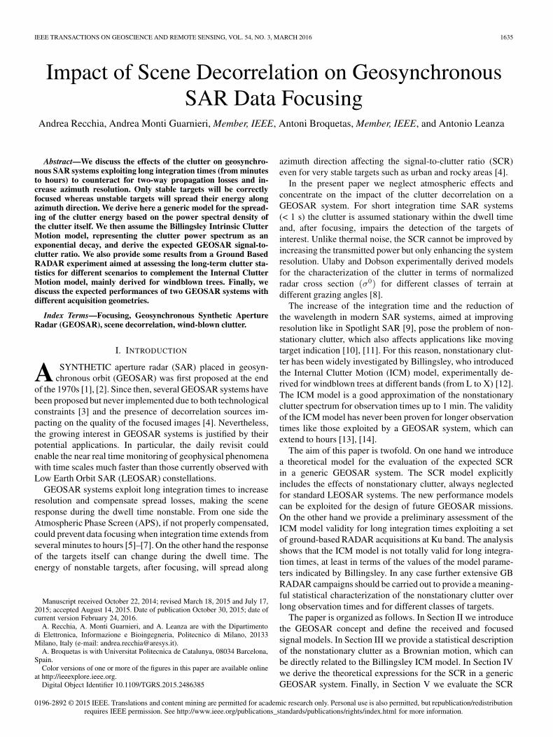
Fig. 1. Acquisition geometry and ground coverage of the continental (red) andregional (green) geosynchronous SAR systems.

TABLE ICOMPARISON BETWEEN MAIN SYSTEM PARAMETERS

OF CONTINENTAL AND TLCOMP SYSTEMS

expressions for two different GEOSAR concepts, assessingtheir robustness in front of the scene decorrelation.

II. GEOSAR CONCEPTS AND SIGNAL MODELS

A. GEOSAR Concepts

Two main GEOSAR concepts have been proposed in liter-ature. The first one achieves continental coverage by meansof a significant orbit inclination [2]. Integration time in theorder of minutes, high power, and quite large antennas areexploited to counteract for the spread losses. According to [3]road-map, such system would require 2020 technologies to beimplemented.

A totally different concept, first proposed in [15], is basedon a negligible orbit inclination, very long integration times,and reduced requirements in terms of power and antenna size,making it suited to be hosted as an additional payload on acommercial telecommunication satellite (TeLecom COMPati-ble concept).

Fig. 1 compares the two GEOSAR concepts in terms of orbit(in an Earth Fixed Reference System) and ground coverage. Thecontinental system would allow to monitor a very large area—say from Equator to midlatitudes of both hemispheres—in anon continuous way. On the contrary the reduced orbit ex-tension of the TLCOMP system would allow the continuousmonitoring—say a low-resolution image every 15 min—of aregion located at midlatitude such as Central Europe.

Table I provides a comparison between the main systemparameters of the GEOSAR concepts. The values for the con-

tinental system were retrieved from [2] and [16] while for theTLCOMP concept we take as reference the system proposed in[17]. GEOSAR systems would be the natural complement tostandard LEOSAR sensors, providing nearly real time monitor-ing of events such landslides, motion of glaciers and volcanoes,ground subsidence and building deformation in urban areas.Furthermore, TLCOMP sensitivity to the atmospheric delaycould be exploited to generate Water Vapor maps over stableland surfaces, which would provide valuable information toNumerical Weather Prediction models.

B. GEOSAR Acquired Signal Model

The impulse response function (IRF) of a GEOSAR systemafter demodulation into base band and range matched filteringcan be written, like for any other SAR, as

hSAR(t, τ ;P)=w(τ ;P)g

[t−R(τ ;P)

2c

]exp

[−j 4π

λR(τ ;P)

](1)

where t is the fast time, τ is the slow time, P is the three-dimensional target location and we have assumed a narrow-band (monochromatic) system with wavelength λ. The firstterm w(τ ;P) is a weighting factor accounting for antennapattern and propagation losses, the second term is the delayedversion of the compressed pulse g(t), and the last term is theslant range phase depending on the sensor-to-target distanceR(τ ;P). The acquired range compressed data are the spa-tially variant convolution between the ground scene and theGEOSAR impulse response

d(t, τ) =

∫L

s(P, τ)hSAR(t, τ ;P)dP (2)

where L represents the area illuminated by the antenna mainlobe and s(P, τ) is the ground scene, assumed both spatiallyand temporally (during the illumination time) variant. Note thatthe scene dependency on the azimuth time is usually neglectedin standard LEOSAR systems due to the very short dwell time.We are interested in assessing the effects of the decorrelatingclutter on the reconstructed scene, assumed spatially impulsivefor simplicity

s(P, τ) = u(τ)δ(P −P0) (3)

where u(τ) is the time varying complex reflectivity of thescene. By substituting (3) in (2) we get the model of theGEOSAR received data for an impulsive decorrelating scene

d(t, τ) = u(τ)hSAR(t, τ ;P0). (4)

C. GEOSAR Focused Signal Model

We assume to reconstruct the imaged scene with the timedomain back-projection algorithm [18]. The BP integral for ageneric scene location can be written as

s(P) =

∫T

d

(R(τ ;P)

2c, τ

)exp

[j4π

λR(τ ;P)

]dτ (5)

RECCHIA et al.: IMPACT OF SCENE DECORRELATION ON GEOSYNCHRONOUS SAR DATA FOCUSING 1637

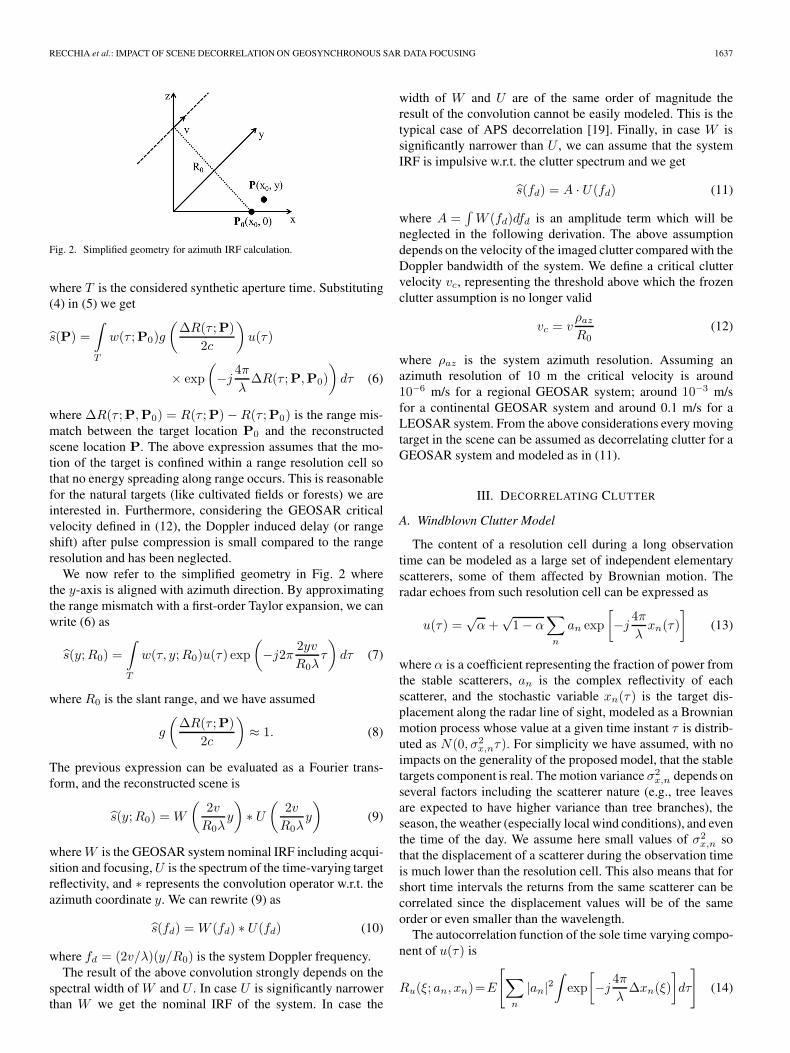
Fig. 2. Simplified geometry for azimuth IRF calculation.

where T is the considered synthetic aperture time. Substituting(4) in (5) we get

s(P) =

∫T

w(τ ;P0)g

(ΔR(τ ;P)

2c

)u(τ)

× exp

(−j

4π

λΔR(τ ;P,P0)

)dτ (6)

where ΔR(τ ;P,P0) = R(τ ;P)−R(τ ;P0) is the range mis-match between the target location P0 and the reconstructedscene location P. The above expression assumes that the mo-tion of the target is confined within a range resolution cell sothat no energy spreading along range occurs. This is reasonablefor the natural targets (like cultivated fields or forests) we areinterested in. Furthermore, considering the GEOSAR criticalvelocity defined in (12), the Doppler induced delay (or rangeshift) after pulse compression is small compared to the rangeresolution and has been neglected.

We now refer to the simplified geometry in Fig. 2 wherethe y-axis is aligned with azimuth direction. By approximatingthe range mismatch with a first-order Taylor expansion, we canwrite (6) as

s(y;R0) =

∫T

w(τ, y;R0)u(τ) exp

(−j2π

2yv

R0λτ

)dτ (7)

where R0 is the slant range, and we have assumed

g

(ΔR(τ ;P)

2c

)≈ 1. (8)

The previous expression can be evaluated as a Fourier trans-form, and the reconstructed scene is

s(y;R0) = W

(2v

R0λy

)∗ U

(2v

R0λy

)(9)

where W is the GEOSAR system nominal IRF including acqui-sition and focusing,U is the spectrum of the time-varying targetreflectivity, and ∗ represents the convolution operator w.r.t. theazimuth coordinate y. We can rewrite (9) as

s(fd) = W (fd) ∗ U(fd) (10)

where fd = (2v/λ)(y/R0) is the system Doppler frequency.The result of the above convolution strongly depends on the

spectral width of W and U . In case U is significantly narrowerthan W we get the nominal IRF of the system. In case the

width of W and U are of the same order of magnitude theresult of the convolution cannot be easily modeled. This is thetypical case of APS decorrelation [19]. Finally, in case W issignificantly narrower than U , we can assume that the systemIRF is impulsive w.r.t. the clutter spectrum and we get

s(fd) = A · U(fd) (11)

where A =∫W (fd)dfd is an amplitude term which will be

neglected in the following derivation. The above assumptiondepends on the velocity of the imaged clutter compared with theDoppler bandwidth of the system. We define a critical cluttervelocity vc, representing the threshold above which the frozenclutter assumption is no longer valid

vc = vρazR0

(12)

where ρaz is the system azimuth resolution. Assuming anazimuth resolution of 10 m the critical velocity is around10−6 m/s for a regional GEOSAR system; around 10−3 m/sfor a continental GEOSAR system and around 0.1 m/s for aLEOSAR system. From the above considerations every movingtarget in the scene can be assumed as decorrelating clutter for aGEOSAR system and modeled as in (11).

III. DECORRELATING CLUTTER

A. Windblown Clutter Model

The content of a resolution cell during a long observationtime can be modeled as a large set of independent elementaryscatterers, some of them affected by Brownian motion. Theradar echoes from such resolution cell can be expressed as

u(τ) =√α+

√1− α

∑n

an exp

[−j

4π

λxn(τ)

](13)

where α is a coefficient representing the fraction of power fromthe stable scatterers, an is the complex reflectivity of eachscatterer, and the stochastic variable xn(τ) is the target dis-placement along the radar line of sight, modeled as a Brownianmotion process whose value at a given time instant τ is distrib-uted as N(0, σ2

x,nτ). For simplicity we have assumed, with noimpacts on the generality of the proposed model, that the stabletargets component is real. The motion variance σ2

x,n depends onseveral factors including the scatterer nature (e.g., tree leavesare expected to have higher variance than tree branches), theseason, the weather (especially local wind conditions), and eventhe time of the day. We assume here small values of σ2

x,n sothat the displacement of a scatterer during the observation timeis much lower than the resolution cell. This also means that forshort time intervals the returns from the same scatterer can becorrelated since the displacement values will be of the sameorder or even smaller than the wavelength.

The autocorrelation function of the sole time varying compo-nent of u(τ) is

Ru(ξ; an, xn)=E

[∑n

|an|2∫exp

[−j

4π

λΔxn(ξ)

]dτ

](14)


where we have neglected the constant (1− α) term and ex-ploited the weak stationarity of the scatterers motion processesand their statistical independence. By exploiting the relation-ship E[exp(jφ)] = exp(−σ2

φ/2) we can rewrite (14) as

Ru

(ξ; an, σ

2x,n

)=∑n

|an|2 exp[−(4π

λ

)2 σ2x,n

2ξ

]. (15)

By assuming that the complex reflectivity an is a set of zeromean, independent random variables with E[|an|2] = Pc, theautocorrelation function can be written as

Ru(ξ) =E{an},{σ2x,n}

{Ru

(ξ; an, σ

2x,n

)}=Pc

∫exp

[−(4π

λ

)2 σ2x,n

2ξ

]f(σ2x,n

)dσ2

x,n (16)

where f(σ2x,n) is the probability density function of the

Brownian motion variance. Finally, the clutter power spectrumcan be written as

|U(fd)|2 = αδ(fd) + (1− α)F {Ru(ξ)} . (17)

The previous expression is quite generic and can lead todifferent clutter power spectrum models such as Gaussianor Power Law. Billingsley showed both experimentally [12]and theoretically [20] that the power spectrum of windblownclutter can be approximated with an exponential decay at neargrazing incidence and over short integration times. The clutterpower spectrum according to Billingsley ICM model can berepresented as

|U(fd)|2 =r

r + 1δ(fd) +

1

r + 1Su(fd) (18)

where r is the ratio of dc power to ac power in the spectrumand the spectral components of the time varying clutter showan exponential decay w.r.t. to the frequency

Su(fd) =βλ

4exp

(−βλ

2|fd|)

(19)

where β is the exponential shape parameter providing the decayrate and

∫|U(fd)|2dfd = 1. Note that (18) and (19) can also be

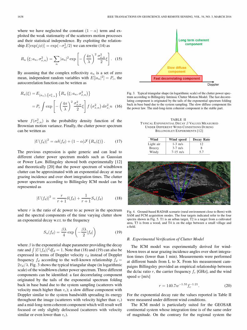
expressed in terms of Doppler velocity vd instead of Dopplerfrequency fd according to the well-known relationship fd =2vd/λ. Fig. 3 shows the typical triangular shape (in logarithmicscale) of the windblown clutter power spectrum. Three differentcomponents can be identified: a fast decorrelating componentoriginated by the tails of the exponential spectrum foldingback in base band due to the system sampling (scatterers withvelocity much higher than vc); a slow diffuse component withDoppler similar to the system bandwidth spreading its energythroughout the image (scatterers with velocity higher than vc)and a mid-long-term coherent component which will result wellfocused or only slightly defocused (scatterers with velocitysimilar or even lower than vc).

Fig. 3. Typical triangular shape (in logarithmic scale) of the clutter power spec-trum according to Billingsley Intrinsic Clutter Motion Model. The fast decorre-lating component is originated by the tails of the exponential spectrum foldingback in base band due to the system sampling. The slow diffuse component fitsthe power law. The mid-long-term coherent component is the stable part.

TABLE IITYPICAL EXPONENTIAL DECAY β VALUES MEASURED

UNDER DIFFERENT WIND CONDITIONS DURING

BILLINGSLEY EXPERIMENTS [12]

Fig. 4. Ground-based RADAR scenario (rural environment close to Bern) withSAM and FCM acquisition modes. The four targets indicated refer to the fourspectra shown in Fig. 5. T1 is an urban target, T2 is a target from a cultivatedarea, T3 is from a wood, and T4 is on the edge between a small village anda field.

B. Experimental Verification of Clutter Model

The ICM model was experimentally derived for wind-blown trees at near grazing incidence angles over short integra-tion times (lower than 1 min). Measurements were performedat different bands from L to X. From his measurement cam-paigns Billingsley provided an empirical relationship betweenthe dc/ac ratio r, the carrier frequency fc [GHz], and the windspeed w [m/s]

r = 140.7w−1.55f−1.21c . (20)

For the exponential decay rate the values reported in Table IIwere measured under different wind conditions.

The ICM model is particularly suited for the GEOSARcontinental system whose integration time is of the same orderof magnitude. On the contrary for the regional system the


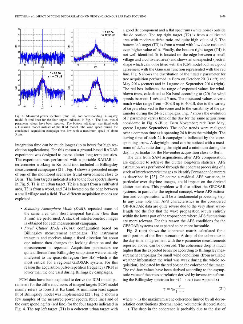
Fig. 5. Measured power spectrum (blue line) and corresponding Billingsleymodel fit (red line) for the four targets indicated in Fig. 4. The fitted modelparameter values have been reported. The bottom left target was fitted witha Gaussian model instead of the ICM model. The wind speed during theconsidered acquisition campaign was low with a maximum speed of about3 m/s.

integration time can be much longer (up to hours for high res-olution applications). For this reason a ground-based RADARexperiment was designed to assess clutter long-term statistics.The experiment was performed with a portable RADAR in-terferometer working in Ku band (not included in Billingsleymeasurement campaigns) [21]. Fig. 4 shows a geocoded imageof one of the monitored scenarios (rural environment close toBern). The four targets indicated refer to the four spectra shownin Fig. 5. T1 is an urban target, T2 is a target from a cultivatedarea, T3 is from a wood, and T4 is located on the edge betweena small village and a field. Two different acquisition modes areexploited:

• Scanning Atmosphere Mode (SAM): repeated scans ofthe same area with short temporal baseline (less than3 min) are performed. A stack of interferometric imagesis obtained for each measurement campaign.

• Fixed Clutter Mode (FCM): configuration based onBillingsley measurement campaigns. The instrumenttransmits and receives along a fixed direction for aboutone minute then changes the looking direction and themeasurement is repeated. Acquisition parameters arequite different from Billingsley setup since we are mainlyinterested to the quasi-dc region (few Hz) which is themost critical for a regional GEOSAR system. For thisreason the acquisition pulse-repetition frequency (PRF) islower than the one used during Billingsley campaigns.

FCM data have been exploited to derive the ICM model pa-rameters for the different classes of imaged targets (ICM modelmainly refers to forest) at Ku band. A minimum least squarefit of Billingsley model was implemented [22]. Fig. 5 shows afew samples of the measured power spectra (blue line) and ofthe corresponding fits (red line) for the four targets indicated inFig. 4. The top left target (T1) is a coherent urban target with

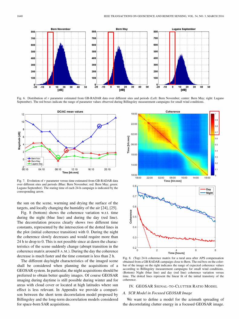
a good dc component and a flat spectrum (white noise) outsidethe dc portion. The top right target (T2) is from a cultivatedarea with moderate dc/ac ratio and quite high value of β. Thebottom left target (T3) is from a wood with low dc/ac ratio andeven higher value of β. Finally, the bottom right target (T4) isnot well identified (it is located on the edge between a smallvillage and a cultivated area) and shows an unexpected spectralshape which cannot be fitted with the ICM model but has a goodagreement with the Gaussian function represented with the redline. Fig. 6 shows the distribution of the fitted r parameter fortree acquisition performed in Bern on October 2013 (left) andMay 2014 (center) and in Lugano on September 2014 (right).The red box indicates the range of expected values for wind-blown trees, calculated at Ku band according to (20) for windspeeds between 1 m/s and 5 m/s. The measured values cover amuch wider range from −20 dB up to 40 dB, due to the varietyof targets observed in the scene and to the variability of the pa-rameter during the 24-h campaigns. Fig. 7 shows the evolutionof r parameter versus time of the day for the same acquisitionsconsidered in Fig. 6 (Blue: Bern November; red: Bern May;green: Lugano September). The dc/ac trends were realignedover a common time axis spanning 24 h from the midnight. Thestaring time of each 24-h campaign is indicated by the corre-sponding arrow. A day/night trend can be noticed with a maxi-mum of dc/ac ratio during the night and a minimum during theday, in particular for the November acquisition close to Bern.

The data from SAM acquisitions, after APS compensation,are exploited to retrieve the clutter long-term statistics. APSestimation was performed through the coherent processing of astack of interferometric images to identify Permanent Scatterersas described in [23]. Of course a residual APS variation, inparticular over daytime images, could impact on the derivedclutter statistics. This problem will also affect the GEOSARsystems, in particular the regional concept, where APS estima-tion and compensation will be a fundamental processing step.In any case note that APS characteristics in the consideredGB-RADAR data are quite severe due to the very short wave-length and the fact that the wave propagation occurs entirelywithin the lower part of the troposphere where APS fluctuationsare more relevant. For this reason the APS conditions for theGESOAR systems are expected to be more favorable.

Fig. 8 (top) shows the coherence matrix calculated for arural portion of the Bern scenario. A drop of the coherence inthe day-time, in agreement with the r parameter measurementsreported above, can be observed. The coherence drop is muchhigher than the expected behavior according to Billingsley mea-surement campaigns for small wind conditions (from availableweather information the wind was weak during the whole ac-quisition), indicated by the red box on the colorbar of the image.The red-box values have been derived according to the asymp-totic value of the cross correlation derived by inverse transform-ing the Billingsley spectrum for γ(t → ∞) (see Appendix)

γ = γ0r

1 + r(21)

where γ0 is the maximum scene coherence limited by all decor-relation contributions (thermal noise, volumetric decorrelation,. . .). The drop in the coherence is probably due to the rise of


Fig. 6. Distribution of r parameter estimated from GB-RADAR data over different sites and periods (Left: Bern November; center: Bern May; right: LuganoSeptember). The red boxes indicate the range of parameter values observed during Billingsley measurement campaigns for small wind conditions.

Fig. 7. Evolution of r parameter versus time estimated from GB-RADAR dataover different sites and periods (Blue: Bern November; red: Bern May; green:Lugano September). The staring time of each 24-h campaign is indicated by thecorresponding arrow.

the sun on the scene, warming and drying the surface of thetargets, and locally changing the humidity of the air [24], [25].

Fig. 8 (bottom) shows the coherence variation w.r.t. timeduring the night (blue line) and during the day (red line).The decorrelation process clearly shows two different timeconstants, represented by the intersection of the dotted lines inthe plot (initial coherence transition) with 0. During the nightthe coherence slowly decreases and would require more than24 h to drop to 0. This is not possible since at dawn the charac-teristics of the scene suddenly change (abrupt transition in thecoherence matrix around 8 A.M.). During the day the coherencedecrease is much faster and the time constant is less than 2 h.

The different day/night characteristics of the imaged sceneshall be considered when planning the acquisitions of aGEOSAR system. In particular, the night acquisitions should bepreferred to obtain better quality images. Of course GEOSARimaging during daytime is still possible during winter and forareas with cloud cover or located at high latitudes where suneffect is less relevant. In Appendix we provide a compari-son between the short term decorrelation model proposed byBillingsley and the long-term decorrelation models consideredfor space-born SAR acquisitions.

Fig. 8. (Top) 24-h coherence matrix for a rural area after APS compensationobtained from a GB RADAR campaign close to Bern. The red box on the color-bar of the image on the right indicates the range of expected coherence valuesaccording to Billingsley measurement campaigns for small wind conditions.(Bottom) Night (blue line) and day (red line) coherence variation versustime. The dotted lines represent the linear fit of the initial transitory of thecoherence.

IV. GEOSAR SIGNAL-TO-CLUTTER RATIO MODEL

A. SCR Model in Focused GEOSAR Image

We want to define a model for the azimuth spreading ofthe decorrelating clutter energy in a focused GEOSAR image.


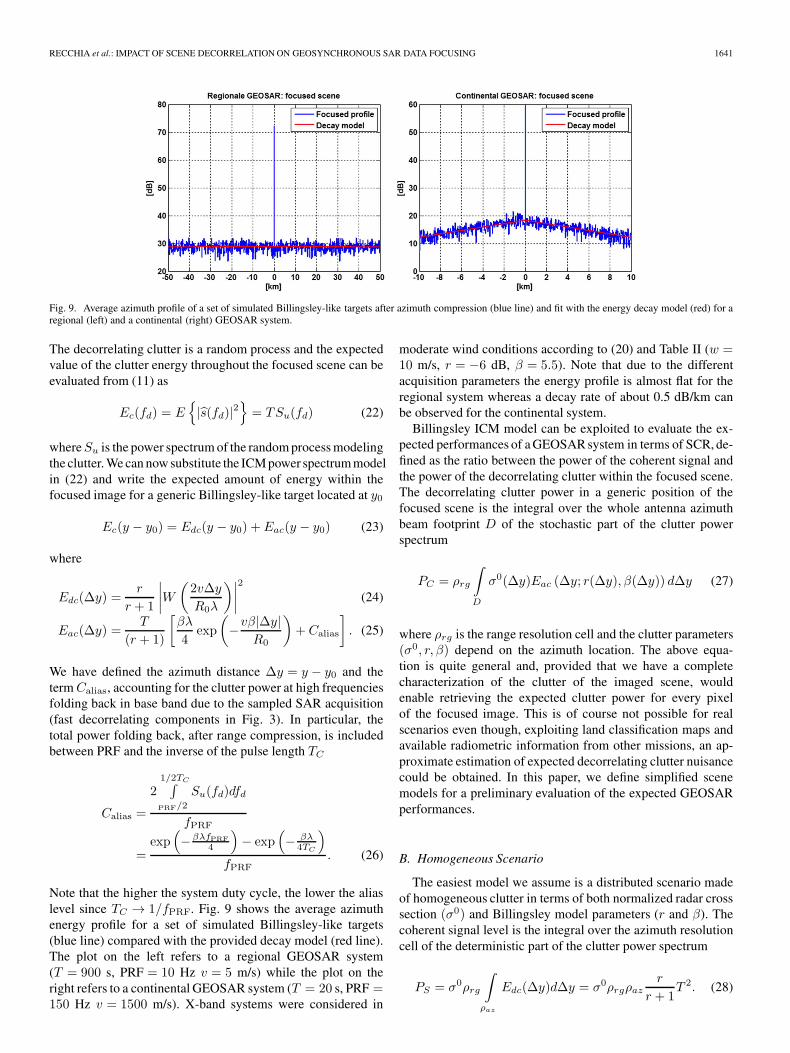
Fig. 9. Average azimuth profile of a set of simulated Billingsley-like targets after azimuth compression (blue line) and fit with the energy decay model (red) for aregional (left) and a continental (right) GEOSAR system.

The decorrelating clutter is a random process and the expectedvalue of the clutter energy throughout the focused scene can beevaluated from (11) as

Ec(fd) = E{|s(fd)|2

}= TSu(fd) (22)

whereSu is the power spectrum of the random process modelingthe clutter. We can now substitute the ICM power spectrum modelin (22) and write the expected amount of energy within thefocused image for a generic Billingsley-like target located at y0

Ec(y − y0) = Edc(y − y0) + Eac(y − y0) (23)

where

Edc(Δy) =r

r + 1

∣∣∣∣W (2vΔy

R0λ

)∣∣∣∣2 (24)

Eac(Δy) =T

(r + 1)

[βλ

4exp

(−vβ|Δy|

R0

)+ Calias

]. (25)

We have defined the azimuth distance Δy = y − y0 and theterm Calias, accounting for the clutter power at high frequenciesfolding back in base band due to the sampled SAR acquisition(fast decorrelating components in Fig. 3). In particular, thetotal power folding back, after range compression, is includedbetween PRF and the inverse of the pulse length TC

Calias =

21/2TC∫PRF/2

Su(fd)dfd

fPRF

=exp

(−βλfPRF

4

)− exp

(− βλ

4TC

)fPRF

. (26)

Note that the higher the system duty cycle, the lower the aliaslevel since TC → 1/fPRF. Fig. 9 shows the average azimuthenergy profile for a set of simulated Billingsley-like targets(blue line) compared with the provided decay model (red line).The plot on the left refers to a regional GEOSAR system(T = 900 s, PRF = 10 Hz v = 5 m/s) while the plot on theright refers to a continental GEOSAR system (T = 20 s, PRF =150 Hz v = 1500 m/s). X-band systems were considered in

moderate wind conditions according to (20) and Table II (w =10 m/s, r = −6 dB, β = 5.5). Note that due to the differentacquisition parameters the energy profile is almost flat for theregional system whereas a decay rate of about 0.5 dB/km canbe observed for the continental system.

Billingsley ICM model can be exploited to evaluate the ex-pected performances of a GEOSAR system in terms of SCR, de-fined as the ratio between the power of the coherent signal andthe power of the decorrelating clutter within the focused scene.The decorrelating clutter power in a generic position of thefocused scene is the integral over the whole antenna azimuthbeam footprint D of the stochastic part of the clutter powerspectrum

PC = ρrg

∫D

σ0(Δy)Eac (Δy; r(Δy), β(Δy)) dΔy (27)

where ρrg is the range resolution cell and the clutter parameters(σ0, r, β) depend on the azimuth location. The above equa-tion is quite general and, provided that we have a completecharacterization of the clutter of the imaged scene, wouldenable retrieving the expected clutter power for every pixelof the focused image. This is of course not possible for realscenarios even though, exploiting land classification maps andavailable radiometric information from other missions, an ap-proximate estimation of expected decorrelating clutter nuisancecould be obtained. In this paper, we define simplified scenemodels for a preliminary evaluation of the expected GEOSARperformances.

B. Homogeneous Scenario

The easiest model we assume is a distributed scenario madeof homogeneous clutter in terms of both normalized radar crosssection (σ0) and Billingsley model parameters (r and β). Thecoherent signal level is the integral over the azimuth resolutioncell of the deterministic part of the clutter power spectrum

PS = σ0ρrg

∫ρaz

Edc(Δy)dΔy = σ0ρrgρazr

r + 1T 2. (28)


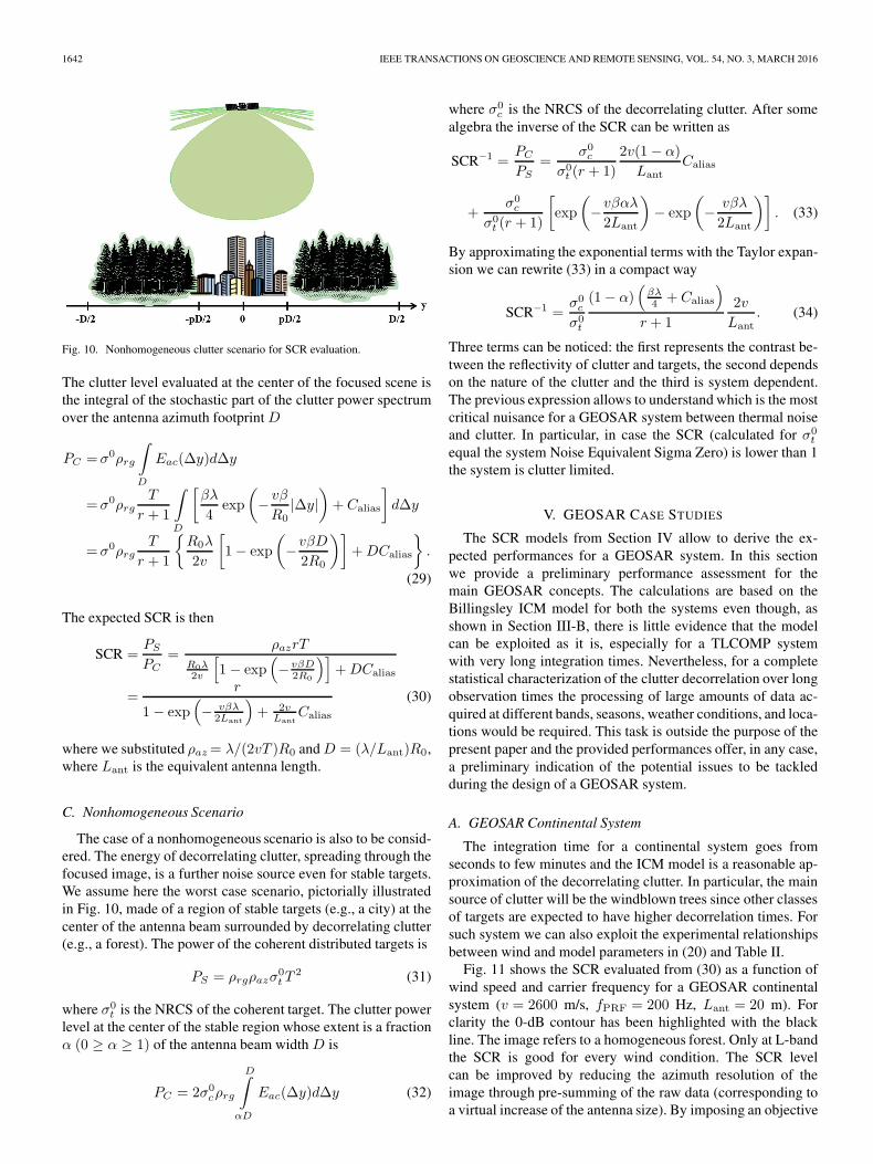
Fig. 10. Nonhomogeneous clutter scenario for SCR evaluation.

The clutter level evaluated at the center of the focused scene isthe integral of the stochastic part of the clutter power spectrumover the antenna azimuth footprint D

PC = σ0ρrg

∫D

Eac(Δy)dΔy

= σ0ρrgT

r + 1

∫D

[βλ

4exp

(− vβ

R0|Δy|

)+ Calias

]dΔy

= σ0ρrgT

r + 1

{R0λ

2v

[1− exp

(−vβD

2R0

)]+DCalias

}.

(29)

The expected SCR is then

SCR =PS

PC=

ρazrT

R0λ2v

[1− exp

(− vβD

2R0

)]+DCalias

=r

1− exp(− vβλ

2Lant

)+ 2v

LantCalias

(30)

where we substituted ρaz= λ/(2vT )R0 and D = (λ/Lant)R0,where Lant is the equivalent antenna length.

C. Nonhomogeneous Scenario

The case of a nonhomogeneous scenario is also to be consid-ered. The energy of decorrelating clutter, spreading through thefocused image, is a further noise source even for stable targets.We assume here the worst case scenario, pictorially illustratedin Fig. 10, made of a region of stable targets (e.g., a city) at thecenter of the antenna beam surrounded by decorrelating clutter(e.g., a forest). The power of the coherent distributed targets is

PS = ρrgρazσ0t T

2 (31)

where σ0t is the NRCS of the coherent target. The clutter power

level at the center of the stable region whose extent is a fractionα (0 ≥ α ≥ 1) of the antenna beam width D is

PC = 2σ0cρrg

D∫αD

Eac(Δy)dΔy (32)

where σ0c is the NRCS of the decorrelating clutter. After some

algebra the inverse of the SCR can be written as

SCR−1 =PC

PS=

σ0c

σ0t (r + 1)

2v(1− α)

LantCalias

+σ0c

σ0t (r + 1)

[exp

(−vβαλ

2Lant

)− exp

(− vβλ

2Lant

)]. (33)

By approximating the exponential terms with the Taylor expan-sion we can rewrite (33) in a compact way

SCR−1 =σ0c

σ0t

(1− α)(

βλ4 + Calias

)r + 1

2v

Lant. (34)

Three terms can be noticed: the first represents the contrast be-tween the reflectivity of clutter and targets, the second dependson the nature of the clutter and the third is system dependent.The previous expression allows to understand which is the mostcritical nuisance for a GEOSAR system between thermal noiseand clutter. In particular, in case the SCR (calculated for σ0

t

equal the system Noise Equivalent Sigma Zero) is lower than 1the system is clutter limited.

V. GEOSAR CASE STUDIES

The SCR models from Section IV allow to derive the ex-pected performances for a GEOSAR system. In this sectionwe provide a preliminary performance assessment for themain GEOSAR concepts. The calculations are based on theBillingsley ICM model for both the systems even though, asshown in Section III-B, there is little evidence that the modelcan be exploited as it is, especially for a TLCOMP systemwith very long integration times. Nevertheless, for a completestatistical characterization of the clutter decorrelation over longobservation times the processing of large amounts of data ac-quired at different bands, seasons, weather conditions, and loca-tions would be required. This task is outside the purpose of thepresent paper and the provided performances offer, in any case,a preliminary indication of the potential issues to be tackledduring the design of a GEOSAR system.

A. GEOSAR Continental System

The integration time for a continental system goes fromseconds to few minutes and the ICM model is a reasonable ap-proximation of the decorrelating clutter. In particular, the mainsource of clutter will be the windblown trees since other classesof targets are expected to have higher decorrelation times. Forsuch system we can also exploit the experimental relationshipsbetween wind and model parameters in (20) and Table II.

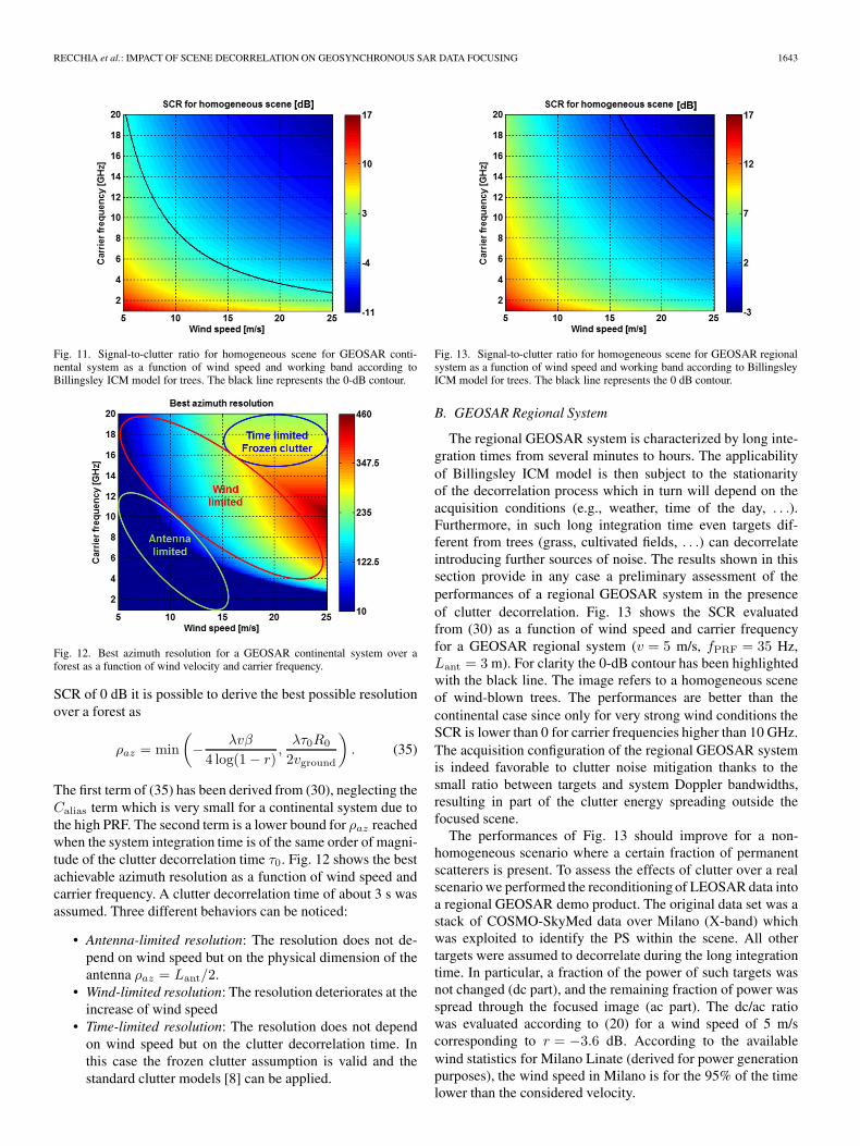
Fig. 11 shows the SCR evaluated from (30) as a function ofwind speed and carrier frequency for a GEOSAR continentalsystem (v = 2600 m/s, fPRF = 200 Hz, Lant = 20 m). Forclarity the 0-dB contour has been highlighted with the blackline. The image refers to a homogeneous forest. Only at L-bandthe SCR is good for every wind condition. The SCR levelcan be improved by reducing the azimuth resolution of theimage through pre-summing of the raw data (corresponding toa virtual increase of the antenna size). By imposing an objective


Fig. 11. Signal-to-clutter ratio for homogeneous scene for GEOSAR conti-nental system as a function of wind speed and working band according toBillingsley ICM model for trees. The black line represents the 0-dB contour.

Fig. 12. Best azimuth resolution for a GEOSAR continental system over aforest as a function of wind velocity and carrier frequency.

SCR of 0 dB it is possible to derive the best possible resolutionover a forest as

ρaz = min

(− λvβ

4 log(1− r),λτ0R0

2vground

). (35)

The first term of (35) has been derived from (30), neglecting theCalias term which is very small for a continental system due tothe high PRF. The second term is a lower bound for ρaz reachedwhen the system integration time is of the same order of magni-tude of the clutter decorrelation time τ0. Fig. 12 shows the bestachievable azimuth resolution as a function of wind speed andcarrier frequency. A clutter decorrelation time of about 3 s wasassumed. Three different behaviors can be noticed:

• Antenna-limited resolution: The resolution does not de-pend on wind speed but on the physical dimension of theantenna ρaz = Lant/2.

• Wind-limited resolution: The resolution deteriorates at theincrease of wind speed

• Time-limited resolution: The resolution does not dependon wind speed but on the clutter decorrelation time. Inthis case the frozen clutter assumption is valid and thestandard clutter models [8] can be applied.

Fig. 13. Signal-to-clutter ratio for homogeneous scene for GEOSAR regionalsystem as a function of wind speed and working band according to BillingsleyICM model for trees. The black line represents the 0 dB contour.

B. GEOSAR Regional System

The regional GEOSAR system is characterized by long inte-gration times from several minutes to hours. The applicabilityof Billingsley ICM model is then subject to the stationarityof the decorrelation process which in turn will depend on theacquisition conditions (e.g., weather, time of the day, . . .).Furthermore, in such long integration time even targets dif-ferent from trees (grass, cultivated fields, . . .) can decorrelateintroducing further sources of noise. The results shown in thissection provide in any case a preliminary assessment of theperformances of a regional GEOSAR system in the presenceof clutter decorrelation. Fig. 13 shows the SCR evaluatedfrom (30) as a function of wind speed and carrier frequencyfor a GEOSAR regional system (v = 5 m/s, fPRF = 35 Hz,Lant = 3 m). For clarity the 0-dB contour has been highlightedwith the black line. The image refers to a homogeneous sceneof wind-blown trees. The performances are better than thecontinental case since only for very strong wind conditions theSCR is lower than 0 for carrier frequencies higher than 10 GHz.The acquisition configuration of the regional GEOSAR systemis indeed favorable to clutter noise mitigation thanks to thesmall ratio between targets and system Doppler bandwidths,resulting in part of the clutter energy spreading outside thefocused scene.

The performances of Fig. 13 should improve for a non-homogeneous scenario where a certain fraction of permanentscatterers is present. To assess the effects of clutter over a realscenario we performed the reconditioning of LEOSAR data intoa regional GEOSAR demo product. The original data set was astack of COSMO-SkyMed data over Milano (X-band) whichwas exploited to identify the PS within the scene. All othertargets were assumed to decorrelate during the long integrationtime. In particular, a fraction of the power of such targets wasnot changed (dc part), and the remaining fraction of power wasspread through the focused image (ac part). The dc/ac ratiowas evaluated according to (20) for a wind speed of 5 m/scorresponding to r = −3.6 dB. According to the availablewind statistics for Milano Linate (derived for power generationpurposes), the wind speed in Milano is for the 95% of the timelower than the considered velocity.


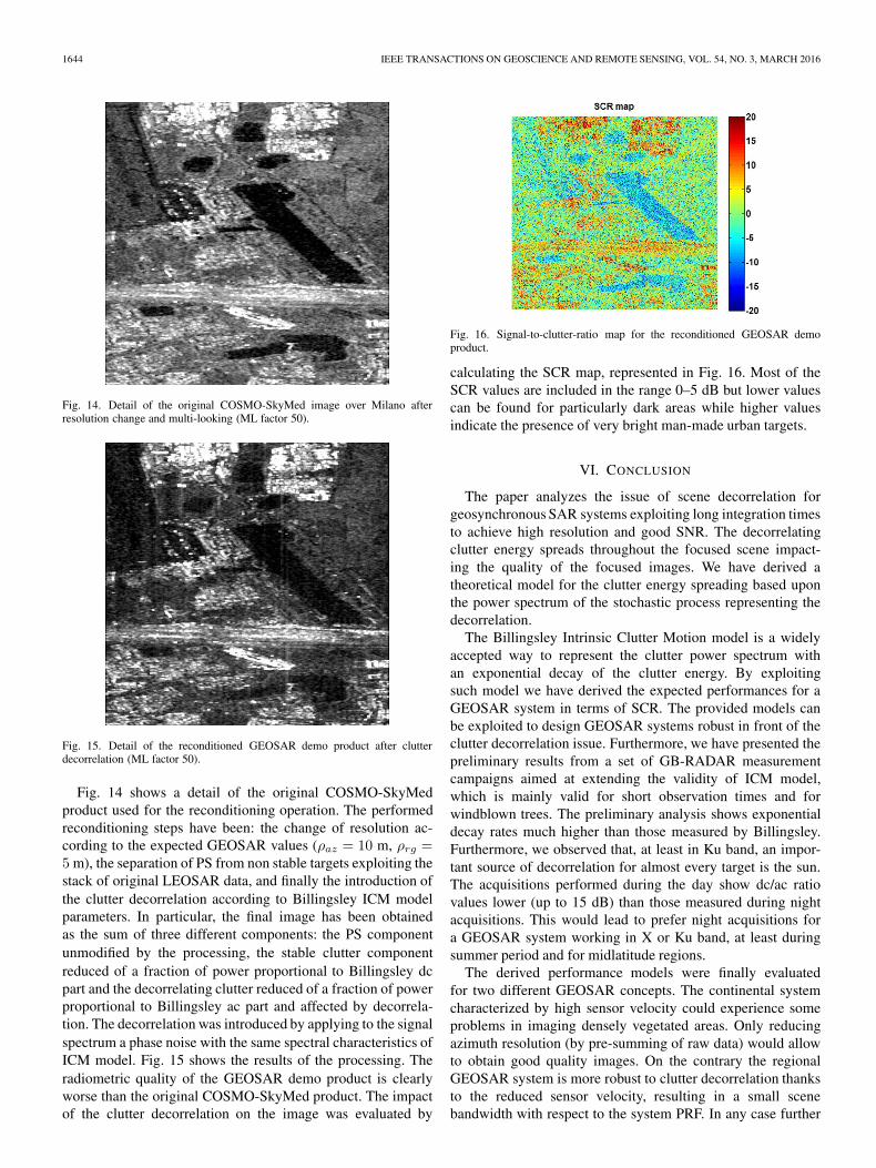
Fig. 14. Detail of the original COSMO-SkyMed image over Milano afterresolution change and multi-looking (ML factor 50).

Fig. 15. Detail of the reconditioned GEOSAR demo product after clutterdecorrelation (ML factor 50).

Fig. 14 shows a detail of the original COSMO-SkyMedproduct used for the reconditioning operation. The performedreconditioning steps have been: the change of resolution ac-cording to the expected GEOSAR values (ρaz = 10 m, ρrg =5 m), the separation of PS from non stable targets exploiting thestack of original LEOSAR data, and finally the introduction ofthe clutter decorrelation according to Billingsley ICM modelparameters. In particular, the final image has been obtainedas the sum of three different components: the PS componentunmodified by the processing, the stable clutter componentreduced of a fraction of power proportional to Billingsley dcpart and the decorrelating clutter reduced of a fraction of powerproportional to Billingsley ac part and affected by decorrela-tion. The decorrelation was introduced by applying to the signalspectrum a phase noise with the same spectral characteristics ofICM model. Fig. 15 shows the results of the processing. Theradiometric quality of the GEOSAR demo product is clearlyworse than the original COSMO-SkyMed product. The impactof the clutter decorrelation on the image was evaluated by

Fig. 16. Signal-to-clutter-ratio map for the reconditioned GEOSAR demoproduct.

calculating the SCR map, represented in Fig. 16. Most of theSCR values are included in the range 0–5 dB but lower valuescan be found for particularly dark areas while higher valuesindicate the presence of very bright man-made urban targets.

VI. CONCLUSION

The paper analyzes the issue of scene decorrelation forgeosynchronous SAR systems exploiting long integration timesto achieve high resolution and good SNR. The decorrelatingclutter energy spreads throughout the focused scene impact-ing the quality of the focused images. We have derived atheoretical model for the clutter energy spreading based uponthe power spectrum of the stochastic process representing thedecorrelation.

The Billingsley Intrinsic Clutter Motion model is a widelyaccepted way to represent the clutter power spectrum withan exponential decay of the clutter energy. By exploitingsuch model we have derived the expected performances for aGEOSAR system in terms of SCR. The provided models canbe exploited to design GEOSAR systems robust in front of theclutter decorrelation issue. Furthermore, we have presented thepreliminary results from a set of GB-RADAR measurementcampaigns aimed at extending the validity of ICM model,which is mainly valid for short observation times and forwindblown trees. The preliminary analysis shows exponentialdecay rates much higher than those measured by Billingsley.Furthermore, we observed that, at least in Ku band, an impor-tant source of decorrelation for almost every target is the sun.The acquisitions performed during the day show dc/ac ratiovalues lower (up to 15 dB) than those measured during nightacquisitions. This would lead to prefer night acquisitions fora GEOSAR system working in X or Ku band, at least duringsummer period and for midlatitude regions.

The derived performance models were finally evaluatedfor two different GEOSAR concepts. The continental systemcharacterized by high sensor velocity could experience someproblems in imaging densely vegetated areas. Only reducingazimuth resolution (by pre-summing of raw data) would allowto obtain good quality images. On the contrary the regionalGEOSAR system is more robust to clutter decorrelation thanksto the reduced sensor velocity, resulting in a small scenebandwidth with respect to the system PRF. In any case further


analysis on the long-term clutter statistics are required for theTLCOMP GEOSAR concept in order to properly account forthe long integration time required by this system.

APPENDIX ATARGETS DECORRELATION MODEL COMPARISON

The coherence between two SAR data x(t) separated by atime interval Δ is defined as

γ =E [x(t)x∗(t+Δ)]√

E[|x(t)|2 |x∗(t+Δ)|

]=

E [x(t)x∗(t+Δ)]

Px=

rx(Δ)

rx(0).

This expression can be related to the ICM model by evaluatingthe autocorrelation of the clutter power spectral density (18)

rx(t) =1

r + 1

1

1 +(

4πtλβ

)2 +r

r + 1.

We can now express the coherence as a function of the theparameters of the ICM model

γ(Δ) =1

r + 1

⎛⎜⎝ 1

1 +(

4πΔλβ

)2 + r

⎞⎟⎠where, as expected, the coherence is unitary for Δ = 0 whileγ(Δ → inf) = r/(r + 1). The dc/ac parameter defines thelong-term coherence, whereas the β parameter describes theshort term behavior. The long-term coherence will be affectedby acquisition condition changes (e.g., wind or day/night).

The dc/ac long-term variations can be described exploitingthe models usually assumed for SAR acquisitions. The firstmodel, valid for long observation times, is [26]

γ(Δt) = exp

(−Δt

τ2

)

τ =λ

4π

√2

σd

derived assuming Brownian motion, that is the displacementsrandomly change with stationary Gaussian increments distrib-uted as N(0, σd). A second model, similar to the first butassuming stationary Brownian motion in increments of velocity(acceleration) is [27]

γ(Δt) = exp

(−(Δt

τ

)2)

τ =λ

4π

√2

σv

where σv is the standard deviation of the velocity increments.Please note that the models have been empirically derived ex-

ploiting spaceborne stacks of interferometric images, with revisit

time of days, whereas in GEOSAR we are interested in decorre-lation times of hours. For this reason, the available GB-RADARcampaigns should be further exploited to derive a model linkingthe short-term decorrelation described by Billingsley with thelong-term models derived from spaceborne SAR.

ACKNOWLEDGMENT

Part of the activities described in the paper was carried outwithin the framework of the ESA-ESTEC funded project: Studyon Utilization of Future Telecom Satellites for Earth Observa-tion. The authors wish to thank T. Strozzi and C. Werner fromGAMMA for performing the radar acquisitions presented inthis paper. The authors also thank M. Belotti and D. Giudicifrom ARESYS for helping in the processing of the GB-RADARdata and in the generation of the GEOSAR demo products.

REFERENCES

[1] K. Tomiyasu, “Synthetic aperture radar in geosynchronous orbit,” in Proc.Antennas Propag. Soc. Int. Symp., 1978, vol. 16, pp. 42–45.

[2] K. Tomiyasu and J. L. Pacelli, “Synthetic aperture radar imaging froman inclined geosynchronous orbit,” IEEE Trans. Geosci. Remote Sens.,vol. GE-21, no. 3, pp. 324–329, Jul. 1983.

[3] W. N. Edelstein, S. N. Madsen, A. Moussessian, and C. Chen, “Conceptsand technologies for synthetic aperture radar from meo and geosynchro-nous orbits,” in Proc. SPIE, 2005, vol. 5659, pp. 195–203.

[4] D. Bruno and S. Hobbs, “Radar imaging from geosynchronous orbit:Temporal decorrelation aspects,” IEEE Trans. Geosci. Remote Sens.,vol. 48, no. 7, pp. 2924–2929, Jul. 2010.

[5] J. Ruiz Rodon, A. Broquetas, A. Monti Guarnieri, and F. Rocca, “Geo-synchronous SAR focusing with atmospheric phase screen retrievaland compensation,” IEEE Trans. Geosci. Remote Sens., vol. 51, no. 8,pp. 4397–4404, Aug. 2013.

[6] C. Hu, T. Long, T. Zeng, F. Liu, and Z. Liu, “The accurate focusingand resolution analysis method in geosynchronous SAR,” IEEE Trans.Geosci. Remote Sens., vol. 49, no. 10, pp. 3548–3563, Oct. 2011.

[7] Y. Tian et al., “Theoretical analysis and verification of time variation ofbackground ionosphere on geosynchronous SAR imaging,” IEEE Geosci.Remote Sens. Lett., vol. 12, no. 4, pp. 721–725, Apr. 2015.

[8] F. T. Ulaby and M. C. Dobson, Handbook of Radar Scattering Statisticsfor Terrain. Dedham, MA, USA: Artech House, 1989.

[9] R. M. M. Walter, G. Carrara, and R. S. Goodman, Spotlight SyntheticAperture Radar: Signal Processing Algorithms. Norwood, MA, USA:Artech House, 1995.

[10] M. Wicks, M. Rangaswamy, R. Adve, and T. Hale, “Space-time adaptiveprocessing: A knowledge-based perspective for airborne radar,” IEEESignal Process. Mag., vol. 23, no. 1, pp. 51–65, Jan. 2006.

[11] D. Pastina and F. Turin, “Exploitation of the cosmo-skymed SAR systemfor gmti applications,” IEEE J. Sel. Topics Appl. Earth Observ. RemoteSens., vol. 8, no. 3, pp. 966–979, Mar. 2015.

[12] J. Billingsley, Low-Angle Radar Land Clutter: Measurements and Empir-ical Models, ser. Radar, Sonar, Navigation and Avionics Bks. Norwich,NY, USA: William Andrew Publ., 2002. [Online]. Available: http://books.google.it/books?id=FEkn0-h7sz0C

[13] A. Recchia, A. Monti Guarnieri, A. Broquetas Ibars, and J. Ruiz Rodon,“Impact of clutter decorrelation on geosynchronous sar,” in Proc. 10thEUSAR, Jun. 2014, pp. 1–4.

[14] J. Ruiz-Rodon, A. Broquetas, E. Makul, A. Monti-Guarnieri, andA. Recchia, “Internal clutter motion impact on the long integrationGEOSAR acquisition,” in Proc. IEEE IGARSS, Jul. 2014, pp. 2343–2346.

[15] C. Prati, F. Rocca, D. Giancola, and A. Guarnieri, “Passive geosynchro-nous SAR system reusing backscattered digital audio broadcasting sig-nals,” IEEE Trans. Geosci. Remote Sens., vol. 36, no. 6, pp. 1973–1976,Nov. 1998.

[16] S. Madsen, W. Edelstein, L. DiDomenico, and J. LaBrecque, “A geosyn-chronous synthetic aperture radar; for tectonic mapping, disaster manage-ment and measurements of vegetation and soil moisture,” in Proc. IEEEIGARSS, 2001, vol. 1, pp. 447–449.

[17] A. Guarnieri, S. Tebaldini, F. Rocca, and A. Broquetas, “Gemini: Geo-synchronous SAR for earth monitoring by interferometry and imaging,”in Proc. IEEE IGARSS, 2012, pp. 210–213.


[18] L. M. H. Ulander, H. Hellsten, and G. Stenstrom, “Synthetic-apertureradar processing using fast factorized back-projection,” IEEE Trans.Aerosp. Electron. Syst., vol. 39, no. 3, pp. 760–776, Jul. 2003.

[19] A. Recchia, A. Monti Guarnieri, A. Broquetas, and J. Ruiz-Rodon, “Ass-esment of atmospheric phase screen impact on geosynchronous SAR,” inProc. IEEE IGARSS, Jul. 2014, pp. 2253–2256.

[20] P. Lombardo and J. B. Billingsley, “A new model for the Doppler spec-trum of windblown radar ground clutter,” in Rec. IEEE Radar Conf., 1999,pp. 142–147.

[21] T. Strozzi, A. Wiesmann, and U. Wegmuller, “Gamma’s portable radarinterferometer,” in Proc. Symp. Deform. Meas. Anal., Lisbon, Portugal,2008, pp. 1–10.

[22] P. Lombardo, M. Greco, F. Gini, A. Farina, and J. Billingsley, “Impactof clutter spectra on radar performance prediction,” IEEE Trans. Aerosp.Electron. Syst., vol. 37, no. 3, pp. 1022–1038, Jul. 2001.

[23] P. Guccione, A. Monti-Guarnieri, and S. Tebaldini, “Stable target de-tection and coherence estimation in interferometric SAR stacks,” IEEETrans. Geosci. Remote Sens., vol. 50, no. 8, pp. 3171–3178, Aug. 2012.

[24] L. Iannini and A. Guarnieri, “Atmospheric phase screen in ground-basedradar: Statistics and compensation,” IEEE Geosci. Remote Sens. Lett.,vol. 8, no. 3, pp. 537–541, May 2011.

[25] F. De Zan, M. Zonno, P. López-Dekker, and A. Parizzi, “Phase inconsis-tencies and water effects in SAR interferometric stacks,” in Proc. FringeWorkshop, 2015, pp. 1–30.

[26] F. Rocca, “Modeling interferogram stacks,” IEEE Trans. Geosci. RemoteSens., vol. 45, no. 10, pp. 3289–3299, Oct. 2007.

[27] H. Zebker and J. Villasenor, “Decorrelation in interferometric radarechoes,” IEEE Trans. Geosci. Remote Sens., vol. 30, no. 5, pp. 950–959,Sep. 1992.

Andrea Recchia was born in Bergamo, Italy, onJuly 7, 1983. He received the master’s degree intelecommunication engineering from Politecnico diMilano, Milano, Italy, in 2008, and the Ph.D. degreeaimed at assessing the feasibility of a novel geosyn-chronous SAR system in the presence of scene andAPS decorrelation, in 2015.

Since 2008 he joined Aresys, a PoliMI spin-off,specialized in radar and geophysics remote sensingsolutions. He is currently part of the SAR R&D teamwith particular interest in SAR data processing, SAR

data quality assessment, and future missions design and evaluation. In 2009 hejoined the Synthetic Aperture Radar study team at Dipartimento di Elettronica,Informazione e Bioingegneria, Politecnico di Milano.

Andrea Monti Guarnieri (M’07) received theM.Sc. degree in electronic engineering from Politec-nico de Milano, Milano, Italy, in 1988.

He had been an Assistant Professor and FullProfessor habilitation within Dipartimento di Elet-tronica, Informazione e Bioingegneria, Politecnicode Milano. He has been teaching several courses ondigital and statistical signal and image processing,telecommunications, and Radar. Almost 40 years ofprofessional activities in SAR systems design andprocessing led him in 2003 to found Aresys, a PoliMI

spin-off, specialized in radar and geophysics remote sensing solutions, then heserved as the President up to 2015. His current interests focus on processingand calibration of ground, airborne and spaceborne SAR, multi-baseline inter-ferometric and MIMO configurations, and geosynchronous SAR.

Prof. Monti Guarnieri coauthored over 200 scientific publications, of which45 international peer-reviewed publications, (H-Index 23, 2600 citations);he was awarded three Best Paper in international symposia (IGARSS ’89,EUSAR 2004, EUSAR 2012), and he is a coauthor of four patents. He is areviewer of journals in remote sensing, signal processing, image processing,geophysics, geodynamics, and antennas and propagations, and he has beenin many technical boards of SAR and RADAR conferences. In 2014 he wasappointed by the board of directors member of Technical-scientific Committeeof Italian Space Agency (ASI).

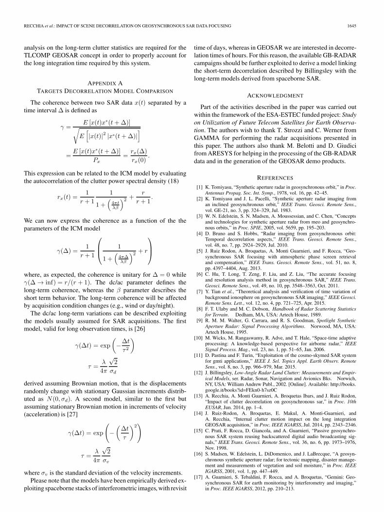
Antoni Broquetas (S’84–M’90) was born inBarcelona, Spain, in 1959. He received the Ingenierodegree in telecommunication engineering from theUniversitat Politecnica de Catalunya (UPC), in 1985,and the Doctor Ingeniero degree in telecommunica-tions engineering for his work on microwave tomog-raphy from UPC, in 1989.

In 1986 he was a Research Assistant in thePortsmouth Polytechnic (U.K.) involved in propaga-tion studies. In 1987 he joined the Department ofSignal Theory and Communications of the School of

Telecommunication Engineering of the UPC in Barcelona.In 1991 he started the remote sensing research activities at UPC working

on the interferometric applications of space-borne synthetic aperture radars.From 1998 to 2002 he was a Subdirector of Research at the Institute ofGeomatics in Barcelona. From 1999 he is a Full Professor in the UPC involvedin research on radar imaging and remote sensing. From 2003 to 2006 he wasthe Director of the Signal Theory and Communications Department at UPC. Hehas published more than 170 papers on microwave tomography, Radar, ISARand SAR systems, SAR processing, and interferometry.

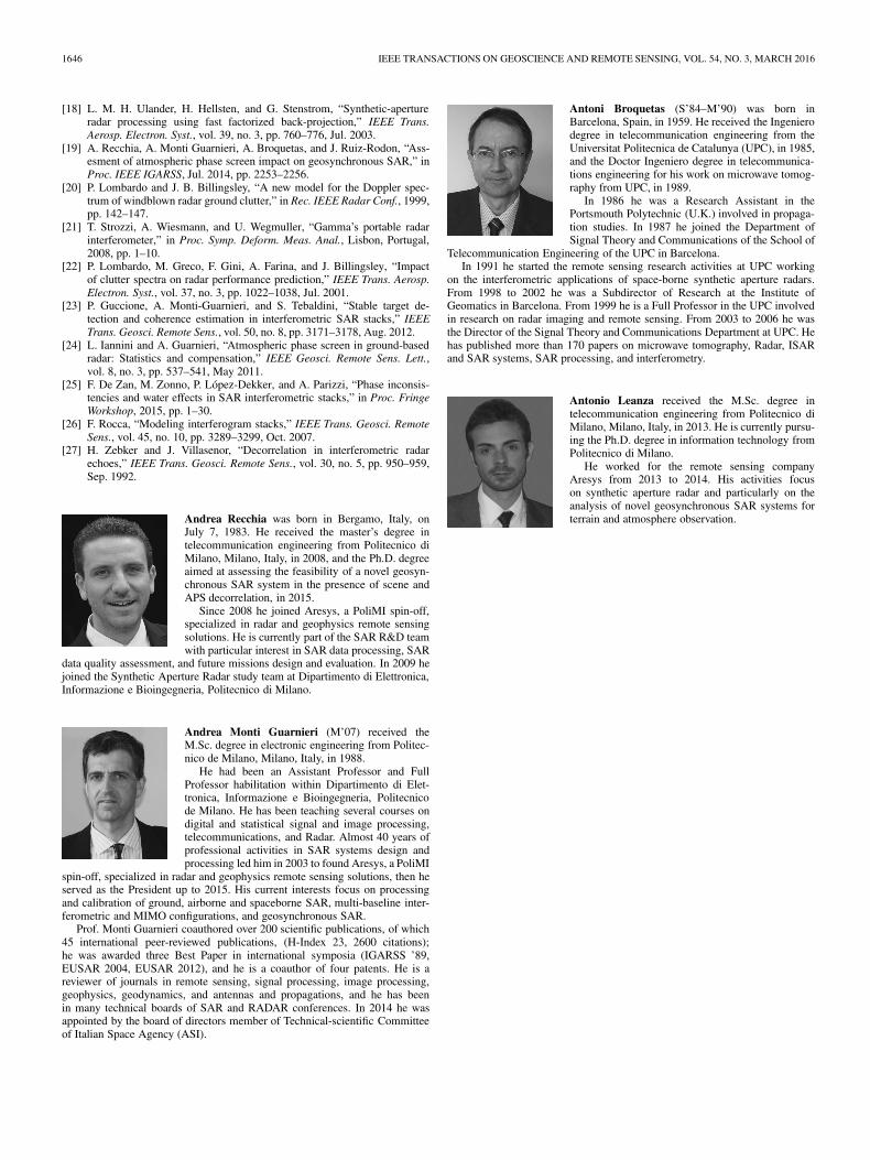
Antonio Leanza received the M.Sc. degree intelecommunication engineering from Politecnico diMilano, Milano, Italy, in 2013. He is currently pursu-ing the Ph.D. degree in information technology fromPolitecnico di Milano.

He worked for the remote sensing companyAresys from 2013 to 2014. His activities focuson synthetic aperture radar and particularly on theanalysis of novel geosynchronous SAR systems forterrain and atmosphere observation.

Documents

Impact of Scene Decorrelation on Geosynchronous SAR … · Impact of Scene Decorrelation on Geosynchronous SAR Data ... We then assume the Billingsley Intrinsic Clutter Motion model,