Embed Size (px)
Citation preview
Statistical Science2017, Vol. 32, No. 3, 405–431DOI: 10.1214/17-STS611© Institute of Mathematical Statistics, 2017
Importance Sampling: Intrinsic Dimensionand Computational CostS. Agapiou, O. Papaspiliopoulos, D. Sanz-Alonso and A. M. Stuart
Abstract. The basic idea of importance sampling is to use independent sam-ples from a proposal measure in order to approximate expectations with re-spect to a target measure. It is key to understand how many samples are re-quired in order to guarantee accurate approximations. Intuitively, some no-tion of distance between the target and the proposal should determine thecomputational cost of the method. A major challenge is to quantify this dis-tance in terms of parameters or statistics that are pertinent for the practitioner.The subject has attracted substantial interest from within a variety of com-munities. The objective of this paper is to overview and unify the resultingliterature by creating an overarching framework. A general theory is pre-sented, with a focus on the use of importance sampling in Bayesian inverseproblems and filtering.
Key words and phrases: Importance sampling, notions of dimension, smallnoise, absolute continuity, inverse problems, filtering.
1. INTRODUCTION
1.1 Our Purpose
Our purpose in this paper is to overview variousways of measuring the computational cost of impor-tance sampling, to link them to one another throughtransparent mathematical reasoning, and to create co-hesion in the vast published literature on this subject. Inaddressing these issues, we will study importance sam-pling in a general abstract setting, and then in the par-ticular cases of Bayesian inversion and filtering. These
S. Agapiou is Lecturer, Department of Mathematics andStatistics, University of Cyprus, 1 University Avenue, 2109Nicosia, Cyprus (e-mail: [email protected]).O. Papaspiliopoulos is ICREA Research Professor, ICREA& Department of Economics, Universitat Pompeu Fabra,Ramon Trias Fargas 25-27, 08005 Barcelona, Spain(e-mail: [email protected]).D. Sanz-Alonso is Postdoctoral Research Associate,Division of Applied Mathematics, Brown University,Providence, Rhode Island 02906, USA (e-mail:[email protected]). A. M. Stuart is BrenProfessor of Computing and Mathematical Sciences,Computing and Mathematical Sciences, California Instituteof Technology, Pasadena, California 91125, USA (e-mail:[email protected]).
two application settings are particularly important asthere are many pressing scientific, technological andsocietal problems which can be formulated via inver-sion or filtering. An example of such an inverse prob-lem is the determination of subsurface properties of theEarth from surface measurements; an example of a fil-tering problem is the assimilation of atmospheric mea-surements into numerical weather forecasts. We nowproceed to overview the subject of importance sam-pling, and the perspective on it that is our focus. InSection 1.2, we describe the organization of the paperand our main contributions. Section 1.3 then collectsall the references linked to the material in the intro-duction, as well as other general references on impor-tance sampling. Each subsequent section of the papercontains its own literature review subsection providingfurther elaboration of the literature, and linking it to thedetails of the material that we present in that section.
The general abstract setting in which we work is asfollows. We let μ and π be two probability measureson a measurable space (X ,F) related via the expres-sion
(1.1)dμ
dπ(u) := g(u)
/ ∫X
g(u)π(du).
Here, g is the unnormalised density (or Radon–Niko-dym derivative) of μ with respect to π . Note that the
405
406 AGAPIOU, PAPASPILIOPOULOS, SANZ-ALONSO AND STUART
very existence of the density implies that the target isabsolutely continuous with respect to the proposal; ab-solute continuity will play an important role in our sub-sequent developments.
Importance sampling is a method for using indepen-dent samples from the proposal π to approximatelycompute expectations with respect to the target μ. Theway importance sampling (and more generally MonteCarlo integration methods) is used within Bayesianstatistics and Bayesian inverse problems is as an ap-proximation of the target measure μ by a random prob-ability measure using weighted samples that are gener-ated from π . (This perspective differs from that aris-ing in other disciplines, e.g., in certain applications inmathematical finance, such as option pricing.) Our per-spective is dictated by the need to use the samples toestimate expectations and quantiles of a wide rangeof functions defined on the state space, for example,functions of a single variable or pairs of variables, ormarginal likelihood quantities. The resulting approx-imation is typically called a particle approximation.Our perspective on importance sampling as a proba-bility measure approximation dictates in turn the toolsfor studying its performance. Its computational cost ismeasured by the number of samples required to con-trol the worst error made when approximating expec-tations within a class of test functions. In this article,and following existing foundational work, we primar-ily focus on a total variation metric between randommeasures for assessing the particle approximation er-ror. Intuitively, the size of the error is related to howfar the target measure is from the proposal measure.We make this intuition precise, and connect the parti-cle approximation error to a key quantity, the secondmoment of dμ/dπ under the proposal, which we de-note by ρ:
ρ = π(g2)
/π(g)2.
As detailed below, ρ is essentially the χ2 divergencebetween the target and the proposal.
The first application of this setting that we study isthe linear inverse problem to determine u ∈ X from y
where
(1.2) y = Ku + η, η ∼ N(0,�).
We adopt a Bayesian approach in which we place aprior u ∼ Pu = N(0,�), assume that η is independentof u and seek the posterior u|y ∼ Pu|y . We study im-portance sampling with Pu|y being the target μ and Pu
being the proposal π .
The second application is the linear filtering prob-lem of sequentially updating the distribution of vj ∈Xgiven {yi}ji=1 where
vj+1 = Mvj + ξj ,
ξj ∼ N(0,Q), j ≥ 0,
yj+1 = Hvj+1 + ζj+1,
ζj+1 ∼ N(0,R), j ≥ 0.
(1.3)
We assume that the problem has a Markov structure.We study the approximation of one step of the filter-ing update by means of particles, building on the studyof importance sampling for the linear inverse prob-lem. To this end, it is expedient to work on the prod-uct space X × X , and consider importance samplingfor (vj , vj+1) ∈ X ×X . It then transpires that, for twodifferent proposals, which are commonly termed thestandard proposal and the optimal proposal, the cost ofone step of particle filtering may be understood by thestudy of a linear inverse problem on X ; we show thisfor both proposals, and then use the link to an inverseproblem to derive results about the cost of particle fil-ters based on these two proposals.
The linear Gaussian models that we study can—andtypically should—be treated by direct analytic calcula-tions or efficient simulation of Gaussians. However, itis possible to analytically study the dependence of ρ onkey parameters within these model classes, and further-more they are flexible enough to incorporate formula-tions on function spaces, and their finite dimensionalapproximations. Thus, they are an excellent frameworkfor obtaining insight into the performance of impor-tance sampling for inverse problems and filtering.
For the abstract importance sampling problem, wewill relate ρ to a number of other natural quanti-ties. These include the effective sample size ess, usedheuristically in many application domains, and a vari-ety of distance metrics between π and μ. Since the ex-istence of a density between target and proposal playsan important role in this discussion, we will also inves-tigate what happens as this absolute continuity prop-erty breaks down. We study this first in high dimen-sional problems, and second in singular parameter lim-its (by which we mean limits of important parametersdefining the problem). The ideas behind these two dif-ferent ways of breaking absolute continuity are pre-sented in the general framework, and then substantiallydeveloped in the inverse problem and filtering settings.The motivation for studying these limits can be appre-ciated by considering the two examples mentioned at

IMPORTANCE SAMPLING 407
the start of this introduction: inverse problems from theEarth’s subsurface, and filtering for numerical weatherprediction. In both cases, the unknown which we aretrying to determine from data is best thought of as aspatially varying field for subsurface properties such aspermeability, or atmospheric properties, such as tem-perature. In practice, the field will be discretized andrepresented as a high dimensional vector, for computa-tional purposes, but for these types of application thestate dimension can be of order 109. Furthermore, ascomputer power advances there is pressure to resolvemore physics, and hence for the state dimension to in-crease. Thus, it is important to understand infinite di-mensional problems, and sequences of approximatingfinite dimensional problems which approach the infi-nite dimensional limit. A motivation for studying sin-gular parameter limits arises, for example, from prob-lems in which the noise is small and the relevant log-likelihoods scale inversely with the noise variance.
This paper aims in particular to contribute towards abetter understanding of the recurrent claim that impor-tance sampling suffers from the curse of dimensional-ity. Whilst there is some empirical truth in this state-ment, there is a great deal of confusion in the literatureabout what exactly makes importance sampling hard.In fact, such a statement about the role of dimensionis vacuous unless “dimension” is defined precisely. Wewill substantially clarify these issues in the contexts ofinverse problems and filtering. Throughout this paper,we use the following conventions:
• State space dimension is the dimension of the mea-surable space where the measures μ and π are de-fined. We will be mostly interested in the case wherethe measurable space X is a separable Hilbert space,in which case the state space dimension is the cardi-nality of an orthonormal basis of the space. In thecontext of inverse problems and filtering, the statespace dimension is the dimension of the unknown.
• Data space dimension is the dimension of the spacewhere the data lives.
• Nominal dimension is the minimum of the statespace dimension and the data state dimension.
• Intrinsic dimension: we will use two notions of in-trinsic dimension for linear Gaussian inverse prob-lems, denoted by efd and τ . These combine state/data dimension and small noise parameters. Theycan be interpreted as a measure of how informativethe data is relative to the prior.
We show that the intrinsic dimensions are naturalwhen studying the computational cost of importance
sampling for inverse problems. In particular, we showhow these intrinsic dimensions relate to the parame-ter ρ introduced above, a parameter that we show tobe central to the computational cost, and to the break-down of absolute continuity. Finally, we apply our un-derstanding of linear inverse problems to particle fil-ters, translating the results from one to the other viaan interesting correspondence between the two prob-lems, for both standard and optimal proposals, that wedescribe here. In studying these quantities, and theirinter-relations, we aim to achieve the purpose set out atthe start of this introduction.
1.2 Organization of the Paper and MainContributions
Section 2 describes importance sampling in abstractform. In Sections 3 and 4, the linear Gaussian inverseproblem and the linear Gaussian filtering problem arestudied. Our aim is to provide a digestible narrative,and hence all proofs—and all technical matters relatedto studying measures in infinite dimensional spaces—are left to the Supplementary Material [4].
Further to providing a unified narrative of the exist-ing literature, this paper contains some original contri-butions that shed new light on the use of importancesampling for inverse problems and filtering. Our mainnew results are:
• Theorem 2.1 bounds the error of importance sam-pling for bounded test functions. The main appealof this theorem is its nonasymptotic nature, togetherwith its clean interpretation in terms of: (i) the keyquantity ρ; (ii) effective sample size; (iii) metricsbetween probability measures; (iv) existing asymp-totic results. According to the perspective on impor-tance sampling as an approximation of one probabil-ity measure by another, the metric used in Theorem2.1 is natural and it has already been used in im-portant theoretical developments in the field as wediscuss in Section 2.5. On the other hand, the re-sult is less useful for quantifying the error for a spe-cific test function of interest, such as linear, bilin-ear or quadratic functions, typically used for com-puting moments and covariances. We discuss exten-sions and generalizations in Section 2.
• Theorem 3.8 studies importance sampling for in-verse problems. It is formulated in the linear Gaus-sian setting to allow a clear and full develop-ment of the connections that it makes betweenheretofore disparate notions. In particular, we high-light the following. (i) It provides the first clear

408 AGAPIOU, PAPASPILIOPOULOS, SANZ-ALONSO AND STUART
connection between finite intrinsic dimension andabsolute continuity between posterior and prior.(ii) It demonstrates the relevance of the intrinsicdimension—rather than the state space or the nom-inal dimension—in the performance of importancesampling, by linking the intrinsic dimension and theparameter ρ; thus, it shows the combined effect ofthe prior, the forward map and the noise model in theefficacy of the method. (iii) It provides theoreticalsupport for the use of algorithms based on impor-tance sampling for posterior inference in functionspace, provided that the intrinsic dimension is finiteand the value of ρ is moderate.
• Theorems 4.2 and 4.3 are proved by studying the in-verse problem at the heart of importance samplingbased particle filters. These theorems, together withTheorem 4.5 and Example 4.6, provide an improvedunderstanding of the advantages of the optimal pro-posal over the standard proposal in the context offiltering.
1.3 Literature Review
In this subsection, we provide a historical review ofthe literature in importance sampling. Each of the fol-lowing Sections 2, 3 and 4 will contain a further liter-ature review subsection providing detailed referenceslinked explicitly to the theory as outlined in those sec-tions.
Early developments of importance sampling as amethod to reduce the variance in Monte Carlo estima-tion date back to the early 1950s [47, 48]. In particular,the paper [48] demonstrates how to optimally choosethe proposal density for given test function φ and targetdensity. Standard text book references for importancesampling include [33] and [71]. Important method-ological improvements were introduced in [66, 72, 82]and [96]. A modern view of importance sampling inthe general framework (1.1) is given in [22]. A com-prehensive description of Bayesian inverse problemsin finite state/data space dimensions can be found in[49], and its formulation in infinite dimensional spacesin [30, 60–62, 95]. Text books overviewing the subjectof filtering and particle filters include [6, 31], and thearticle [27] provides a readable introduction to the area.For an up-to-date and in-depth survey of nonlinear fil-tering, see [28]. The linear Gaussian inverse problemand the linear Gaussian filtering problem have been ex-tensively studied because they arise naturally in manyapplications, lead to considerable algorithmic tractabil-ity, and provide theoretical insight. For references con-cerning linear Gaussian inverse problems, see [39, 53,
64, 74]. The linear Gaussian filter—the Kalman filter—was introduced in [51]; see [59] for further analysis.The inverse problem of determining subsurface prop-erties of the Earth from surface measurements is dis-cussed in [81], while the filtering problem of assimilat-ing atmospheric measurements for numerical weatherprediction is discussed in [52].
The key role of ρ, the second moment of the Radon–Nikodym derivative between the target and the pro-posal, has long been acknowledged [70, 83]. The cru-cial question of how to choose a proposal measure thatleads to small value of ρ has been widely studied, andwe refer to [67] and references therein. In this vein,our theory in Sections 3 and 4 shows precise condi-tions that guarantee ρ < ∞ in inverse problems andfiltering settings, in terms of well-defined basic con-cepts such as absolute continuity of the target with re-spect to the proposal. Our study of importance sam-pling for inverse problems in Section 3 is limited to thechoice of prior as proposal, which is of central theo-retical relevance. In practice, however, more sophisti-cated proposals are often used, potentially leading toreduced parameter ρ; two novel ideas include the im-plicit sampling method described in [78], and the useof proposals based on the ensemble Kalman filter sug-gested in [65]. The value of ρ is known to be asymptot-ically linked to the effective sample size [56, 57, 70].Recent justification for the use of the effective samplesize within particle filters is given in [101]. We pro-vide a further nonasymptotic justification of the rele-vance of ρ through its appearance in error bounds onthe error in importance sampling; a relevant related pa-per is [26] which proved nonasymptotic bounds on theerror in the importance-sampling based particle filteralgorithm. In this paper, we will also bound the im-portance sampling error in terms of different notionsof distance between the target and the proposal mea-sures. Our theory is based on the χ2 divergence—as in[20]—while the recent complementary analysis of im-portance sampling in [19] highlights the advantages ofthe Kullback–Leibler divergence; a useful overview ofthe subject of distances between probability measuresis [43].
We formulate problems in both finite dimensionaland infinite dimensional state spaces. We refer to [50]for a modern presentation of probability appropriatefor understanding the material in this article. Some ofour results are built on the rich area of Gaussian mea-sures in Hilbert space; we include all the required back-ground in the Supplementary Material, and referencesare included there. However, we emphasize that the

IMPORTANCE SAMPLING 409
presentation in the main body of the text is designedto keep technical material to a minimum and to be ac-cessible to readers who are not versed in the theoryof probability in infinite dimensional spaces. Absolutecontinuity of the target with respect to the proposal—or the existence of a density of the target with respectto the proposal—is central to our developments. Thisconcept also plays a pivotal role in the understandingof Markov chain Monte Carlo (MCMC) methods inhigh and infinite dimensional spaces [97]. A key ideain MCMC is that breakdown of absolute continuity onsequences of problems of increasing state space dimen-sion is responsible for poor algorithmic performancewith respect to increasing dimension; this should beavoided if possible, such as for problems with a well-defined infinite dimensional limit [25]. Similar ideaswill come into play in this paper.
As well as the breakdown of absolute continuitythrough increase in dimension, small noise limits canalso lead to sequences of proposal/target measureswhich are increasingly close to mutually singular andfor which absolute continuity breaks down. Smallnoise regimes are of theoretical and computational in-terest for both inverse problems and filtering. For in-stance, in inverse problems there is a growing inter-est in the study of the concentration rate of the pos-terior in the small observational noise limit; see [2, 5,53–55, 84, 100]. In filtering and multiscale diffusions,the analysis and development of improved proposals insmall noise limits is an active research area [37, 78, 94,99, 104].
In order to quantify the computational cost of a prob-lem, a recurrent concept is that of intrinsic dimen-sion. Several notions of intrinsic dimension have beenused in different fields, including dimension of learn-ing problems [12, 102, 103], of statistical inverse prob-lems [73], of functions in the context of quasi MonteCarlo (QMC) integration in finance applications [16,58, 79] and of data assimilation problems [23]. Theunderlying theme is that in many application areaswhere models are formulated in high dimensional statespaces, there is often a small subspace which capturesmost of the features of the system. It is the dimensionof this subspace that effects the cost of the problem.The recent subject of active subspaces shows promisein finding such low dimensional subspace of interestin certain applications [24]. In the context of inverseproblems, the paper [8] proposed a notion of intrin-sic dimension that was shown to have a direct con-nection with the performance of importance sampling.We introduce a further notion of intrinsic dimension
for Bayesian inverse problems which agrees with thenotion of effective number of parameters used in ma-chine learning and statistics [12]. We also establish thatthis notion of dimension and the one in [8] are finite, orotherwise, at the same time. Both intrinsic dimensionsaccount for three key features of the cost of the inverseproblem: the nominal dimension (i.e., the minimum ofthe dimension of the state space and the data), the sizeof the observational noise and the regularity of the priorrelative to the observation noise. Varying the parame-ters related to these three features may cause a break-down of absolute continuity. The deterioration of im-portance sampling in large nominal dimensional lim-its has been widely investigated [8, 11, 88–91]. In par-ticular, the key role of the intrinsic dimension, ratherthan the nominal one, in explaining this deteriorationwas studied in [8]. Here, we study the different be-haviour of importance sampling as absolute continuityis broken in the three regimes above, and we investi-gate whether, in all these regimes, the deterioration ofimportance sampling may be quantified by the variousintrinsic dimensions that we introduce.
We emphasize that, whilst the theory and discus-sion in Section 2 is quite general, the applications toBayesian inverse problems (Section 3) and filtering(Section 4) are in the case of linear problems with addi-tive Gaussian noise. This linear Gaussian setting allowssubstantial explicit calculations and yields consider-able insight. However, empirical evidence related to thebehaviour of filters and Monte Carlo based methodswhen applied to nonlinear problems and non-Gaussiantarget measures suggests that similar ideas may applyin those situations; see [14, 24, 25, 29, 90]. Quantifyingthis empirical experience more precisely is an interest-ing and challenging direction for future study. We notein particular that extensions of the intrinsic dimensionquantity that we employ have been provided in the lit-erature for Bayesian hierarchical non-Gaussian mod-els, more specifically within the so-called deviance in-formation criterion of [93]; see Section 3.5.3 for morediscussion.
1.4 Notation
Given a probability measure ν on a measurable space(X ,F) expectations of a measurable function φ :X →R with respect to ν will be written as both ν(φ) andEν[φ]. When it is clear which measure is being usedwe may drop the suffix ν and write simply E[φ]. Simi-larly, the variance will be written as Varν(φ) and againwe may drop the suffix when no confusion arises from
410 AGAPIOU, PAPASPILIOPOULOS, SANZ-ALONSO AND STUART
doing so. All test functions φ appearing in the paperare assumed to be measurable.
We will be interested in sequences of measures in-dexed by time or by the state space dimension. Theseare denoted with a subscript, for example, νt , νd . Any-thing to do with samples from a measure is denotedwith a superscript: N for the number of samples, andn for the indices of the samples. The ith coordinate ofa vector u is denoted by u(i). Thus, un
t (i) denotes ithcoordinate of the nth sample from the measure of in-terest at time t . Finally, the law of a random variable v
will be denoted by Pv .
2. IMPORTANCE SAMPLING
In Section 2.1, we define importance sampling and inSection 2.2 we demonstrate the role of the second mo-ment of the target-proposal density, ρ; we prove two
nonasymptotic theorems showing O((ρ/N)12 ) conver-
gence rate of importance sampling with respect to thenumber N of particles. Then in Section 2.3.2 we showhow ρ relates to the effective sample size ess as oftendefined by practitioners, whilst in Section 2.3.3 we linkρ to various distances between probability measures.In Section 2.4.1, we highlight the role of the break-down of absolute continuity in the growth of ρ, as thedimension of the space X grows. Section 2.4.2 followswith a similar discussion relating to singular limits ofthe density between target and proposal. Section 2.5contains a literature review and, in particular, sourcesfor all the material in this section.
2.1 General Setting
We consider target μ and proposal π , both probabil-ity measures on the measurable space (X ,F), relatedby (1.1). In many statistical applications, interest liesin estimating expectations under μ, for a collection oftest functions, using samples from π . For a test func-tion φ : X →R such that μ(|φ|) < ∞, the identity
μ(φ) = π(φg)
π(g),
leads to the autonormalized importance sampling esti-mator:
μN(φ) :=1N
∑Nn=1 φ(un)g(un)
1N
∑Nm=1 g(um)
, un ∼ π i.i.d.
(2.1)
=N∑
n=1
wnφ(un)
, wn := g(un)∑Nm=1 g(um)
;
here the wn’s are called the normalized weights. Assuggested by the notation, it is useful to view (2.1) asintegrating a function φ with respect to the randomprobability measure μN := ∑N
n=1 wnδun . Under thisperspective, importance sampling consists of approx-imating the target μ by the measure μN , which is typi-cally called the particle approximation of μ. Note that,while μN depends on the proposal π , we suppress thisdependence for economy of notation. Our aim is to un-derstand the quality of the approximation μN of μ. Inparticular, we would like to know how large to chooseN in order to obtain small error. This will quantify thecomputational cost of importance sampling.
2.2 A Nonasymptotic Bound on ParticleApproximation Error
A fundamental quantity in addressing this issue is ρ,defined by
(2.2) ρ := π(g2)
π(g)2 .
Thus, ρ is the second moment of the Radon–Nikodymderivative of the target with respect to the proposal. TheCauchy–Schwarz inequality shows that π(g)2 ≤ π(g2)
and hence that ρ ≥ 1. Our first nonasymptotic resultshows that, for bounded test functions φ, both the biasand the mean square error (MSE) of the autonormal-ized importance sampling estimator are O(N−1) withconstant of proportionality linear in ρ.
THEOREM 2.1. Assume that μ is absolutely con-tinuous with respect to π , with square-integrable den-sity g, that is, π(g2) < ∞. The bias and MSE of im-portance sampling over bounded test functions may becharacterized as follows:
sup|φ|≤1
∣∣E[μN(φ) − μ(φ)
]∣∣ ≤ 12
Nρ,
and
sup|φ|≤1
E[(
μN(φ) − μ(φ))2] ≤ 4
Nρ.
REMARK 2.2. For a bounded test function |φ| ≤ 1,we trivially get |μN(φ)−μ(φ)| ≤ 2; hence the boundson bias and MSE provided in Theorem 2.1 are usefulonly when they are smaller than 2 and 4, respectively.
The upper bounds stated in this result suggest thatit is good practice to keep ρ/N small in order to ob-tain good importance sampling approximations. Thisheuristic dominates the developments in the remainder
IMPORTANCE SAMPLING 411
of the paper, and in particular our wish to study the be-haviour of ρ in various limits. The result trivially ex-tends to provide bounds on the mean square error forfunctions bounded by any other known bound differentfrom 1. For practical purposes, the theorem is directlyapplicable to instances where importance sampling isused to estimate probabilities, such as in rare eventsimulation. However, its primary role is in providinga bound on the particle approximation error, which isnaturally defined over bounded functions, as is com-mon with weak convergence results. It is also impor-tant to realise that such a result will not hold withoutmore assumptions on the weights for unbounded testfunctions; for example when g has third moment butnot fourth under π , then μ(g2) < ∞, π(g2) < ∞ butthe importance sampling estimator of μ(g2) has infi-nite variance. We return to extensions of the theoremfor unbounded test functions in Section 2.3 below.
2.3 Connections, Interpretations and Extensions
Theorem 2.1 clearly demonstrates the role of ρ, thesecond moment of the target density with respect tothe proposal, in determining the number of samples re-quired to effectively approximate expectations. Here,we link ρ to other quantities used in analysis and mon-itoring of importance sampling algorithms, and we dis-cuss some limitations of thinking entirely in terms of ρ.
2.3.1 Asymptotic consistency. It is interesting tocontrast Theorem 2.1 to a well-known elementaryasymptotic result. First, note that
μN(φ) − μ(φ) = N−1 ∑Nn=1
g(un)π(g)
[φ(un) − μ(φ)]N−1 ∑N
n=1g(un)π(g)
.
Therefore, under the condition π(g2) < ∞, and pro-vided additionally that π(g2φ2) < ∞, an applicationof the Slutsky lemmas gives that
(2.3)
√N
(μN(φ) − μ(φ)
) =⇒ N
(0,
π(g2φ2)
π(g)2
),
where φ := φ − μ(φ).
For bounded |φ| ≤ 1, the only condition needed for ap-pealing to the asymptotic result is π(g2) < ∞. Then(2.3) gives that, for large N and since |φ| ≤ 2,
E[(
μN(φ) − μ(φ))2]
� 4
Nρ,
which is in precise agreement with Theorem 2.1.
2.3.2 Effective sample size. Many practitioners de-fine the effective sample size by the formula
ess :=(
N∑n=1
(wn)2
)−1
= (∑N
n=1 g(un))2∑Nn=1 g(un)2
= NπN
MC(g)2
πNMC(g2)
,
where πNMC is the empirical Monte Carlo random mea-
sure
πNMC := 1
N
N∑n=1
δun, un ∼ π.
By the Cauchy–Schwarz inequality, it follows thatess ≤ N . Furthermore, since the weights lie in [0,1],we have
N∑n=1
(wn)2 ≤
N∑n=1
wn = 1
so that ess ≥ 1. These upper and lower bounds maybe attained as follows. If all the weights are equal, andhence take value N−1, then ess = N , the optimal situ-ation. On the other hand, if exactly k weights take thesame value, with the remainder then zero, ess = k; inparticular the lower bound of 1 is attained if preciselyone weight takes the value 1 and all others are zero.
For large enough N , and provided π(g2) < ∞, thestrong law of large numbers gives
ess ≈ N/ρ.
Recalling that ρ ≥ 1, we see that ρ−1 quantifies theproportion of particles that effectively characterize thesample size, in the large particle size asymptotic. Fur-thermore, by Theorem 2.1, we have that, for large N ,
sup|φ|≤1
E[(
μN(φ) − μ(φ))2]
� 4
ess.
This provides a further justification for the use of essas an effective sample size, in the large N asymptoticregime.
2.3.3 Probability metrics. Intuition tells us that im-portance sampling will perform well when the distancebetween proposal π and target μ is not too large. Fur-thermore, we have shown the role of ρ in measuringthe rate of convergence of importance sampling. It ishence of interest to explicitly link ρ to distance metricsbetween π and μ. In fact, we consider asymmetric di-vergences as distance measures; these are not strictly
412 AGAPIOU, PAPASPILIOPOULOS, SANZ-ALONSO AND STUART
metrics, but certainly represent useful distance mea-sures in many contexts in probability. First, considerthe χ2 divergence, which satisfies
(2.4) Dχ2(μ‖π) := π
([g
π(g)− 1
]2)= ρ − 1.
The Kullback–Leibler divergence is given by
DKL(μ‖π) := π
(g
π(g)log
g
π(g)
),
and may be shown to satisfy
(2.5) ρ ≥ eDKL(μ‖π).
Thus, Theorem 2.1 suggests that the number of parti-cles required for accurate importance sampling scalesexponentially with the Kullback–Leibler divergencebetween proposal and target and linearly with the χ2
divergence.
2.3.4 Beyond bounded test functions. In contrastto Theorem 2.1, the asymptotic result (2.3), estab-lishes the convergence rate N−1/2 (asymptotically) un-der the weaker moment assumption on the test func-tion π(g2φ2) < ∞. It is thus of interest to derivenonasymptotic bounds on the MSE and bias for muchlarger classes of test functions. This can be achievedat the expense of more assumptions on the importanceweights. The next theorem addresses the issue of re-laxing the class of test functions, whilst still deriv-ing nonasymptotic bounds. By including the result, wealso highlight the fact that, whilst ρ plays an importantrole in quantifying the difficulty of importance sam-pling, other quantities may be relevant in the analysisof importance sampling for unbounded test functions.Nonetheless, the sufficiency and necessity of scalingthe number of samples with ρ is understood in certainsettings, as will be discussed in the bibliography at theend of this section.
To simplify the statement, we first introduce the fol-lowing notation. We write mt [h] for the t th central mo-ment with respect to π of a function h : X → R. Thatis,
mt [h] := π(∣∣h(u) − π(h)
∣∣t ).We also define, as above, φ := φ − μ(φ).
THEOREM 2.3. Suppose that φ and g are such thatCMSE defined below is finite:
CMSE := 3
π(g)2 m2[φg]
+ 3
π(g)4 π(|φg|2d) 1
d C1e
2em2e[g] 1e
+ 3
π(g)2(1+ 1
p)π
(|φ|2p) 1p
· C1q
2q(1+ 1p)m2q(1+ 1
p)[g] 1
q .
Then the bias and MSE of importance sampling whenapplied to approximate μ(φ) may be characterized asfollows:∣∣E[
μN(φ) − μ(φ)]∣∣
≤ 1
N
(2
π(g)2 m2[g] 12 m2[φg] 1
2 + 2C12MSE
π(g2)12
π(g)
)
and
E[(
μN(φ) − μ(φ))2] ≤ 1
NCMSE.
The constants Ct > 0, t ≥ 2, satisfy C1tt ≤ t − 1 and
the two pairs of parameters d, e, and p,q are conju-gate pairs of indices satisfying d, e,p, q ∈ (1,∞) andd−1 + e−1 = 1, p−1 + q−1 = 1.
REMARK 2.4. In Bayesian inverse problems,π(g) < ∞ often implies that π(gs) < ∞ for any pos-itive s; we will demonstrate this in a particular casein Section 3. In such a case, Theorem 2.3 combinedwith Hölder’s inequality shows that importance sam-pling converges at rate N−1 for any test function φ
satisfying π(|φ|2+ε) < ∞ for some ε > 0. Note, how-ever, that the constant in the O(N−1) error bound is notreadily interpretable simply in terms of ρ; in particularthe expression necessarily involves moments of g withexponent greater than two.
2.4 Behaviour of the Second Moment ρ
Having demonstrated the importance of ρ, the sec-ond moment of the target-proposal density, we nowshow how it behaves in high dimensional problemsand in problems where there are measure concentra-tion phenomena due to a small parameter in the likeli-hood. These two limits will be of importance to us insubsequent sections of the paper, where the small pa-rameter measure concentration effect will arise due tohigh quality data.
2.4.1 High state space dimension and absolutecontinuity. The preceding three subsections have de-monstrated how, when the target is absolutely continu-ous with respect to the proposal, importance samplingconverges as the square root of ρ/N . It is thus naturalto ask if, and how, this desirable convergence breaksdown for sequences of target and proposal measures
IMPORTANCE SAMPLING 413
which become increasingly close to singular. To thisend, suppose that the underlying space is the Carte-sian product Rd equipped with the corresponding prod-uct σ -algebra, the proposal is a product measure andthe un-normalized weight function also has a productform, as follows:
πd(du) =d∏
i=1
π1(du(i)
),
μd(du) =d∏
i=1
μ1(du(i)
),
gd(u) = exp
{−
d∑i=1
h(u(i)
)},
for probability measures π1,μ1 on R and h : R → R+
(and we assume it is not constant to remove the triv-ial case μ1 = π1). We index the proposal, target, den-sity and ρ with respect to d since interest here lies inthe limiting behaviour as d increases. In the setting of(1.1), we now have
(2.6) μd(du) ∝ gd(u)πd(du).
By construction, gd has all polynomial moments un-der πd and importance sampling for each d has thegood properties developed in the previous sections. Itis also fairly straightforward to see that μ∞ and π∞are mutually singular when h is not constant: one wayto see this is to note that
1
d
d∑i=1
u(i)
has a different almost sure limit under μ∞ and π∞.Two measures cannot be absolutely continuous un-less they share the same almost sure properties. There-fore, μ∞ is not absolutely continuous with respect toπ∞ and importance sampling is undefined in the limitd = ∞. As a consequence, we should expect to see adegradation in its performance for large state space di-mension d .
To illustrate this degradation note that under theproduct structure (2.6), we have ρd = (ρ1)
d . Further-more, ρ1 > 1 (since h is not constant). Thus, ρd growsexponentially with the state space dimension suggest-ing, when combined with Theorem 2.1, that exponen-tially many particles are required, with respect to di-mension, to make importance sampling accurate.
It is important to realise that it is not the productstructure per se that leads to the collapse, rather thelack of absolute continuity in the limit of infinite state
space dimension. Thinking about the role of high di-mensions in this way is very instructive in our un-derstanding of high dimensional problems, but is verymuch related to the setting in which all the coordinatesof the problem play a similar role. This does not happenin many application areas. Often there is a diminishingresponse of the likelihood to perturbations in growingcoordinate index. When this is the case, increasing thestate space dimension has only a mild effect in the costof the problem, and it is possible to have well-behavedinfinite dimensional limits; we will see this perspectivein Sections 3.1, 3.2 and 3.3 for inverse problems, andSections 4.1, 4.2 and 4.3 for filtering.
2.4.2 Singular limits. In the previous subsection,we saw an example where for high dimensional statespaces the target and proposal became increasinglyclose to being mutually singular, resulting in ρ whichgrows exponentially with the state space dimension. Inthis subsection, we observe that mutual singularity canalso occur because of small parameters in the unnor-malized density g appearing in (1.1), even in problemsof fixed dimension; this will lead to ρ which grows al-gebraically with respect to the small parameter. To un-derstand this situation, let X = R and consider (1.1) inthe setting where
gε(u) = exp(−ε−1h(u)
),
where h : R → R+. We will write gε and ρε to high-
light the dependence of these quantities on ε. Fur-thermore assume, for simplicity, that h is twice dif-ferentiable and has a unique minimum at u�, and thath′′(u�) > 0. Assume, in addition, that π has a Lebesguedensity with bounded first derivative. Then the Laplacemethod shows that
E exp(−2ε−1h(u)
) ≈ exp(−2ε−1h
(u�))√ 2πε
2h′′(u�)
and that
E exp(−ε−1h(u)
) ≈ exp(−ε−1h
(u�))√ 2πε
h′′(u�).
It follows that
ρε ≈√
h′′(u�)
4πε.
Thus, Theorem 2.1 indicates that the number of parti-cles required for importance sampling to be accurate
should grow at least as fast as ε− 12 .
414 AGAPIOU, PAPASPILIOPOULOS, SANZ-ALONSO AND STUART
2.5 Discussion and Connection to Literature
2.5.1 Metrics between random probability mea-sures. In Section 2.1, we introduced the importancesampling approximation of a target μ using a proposalπ , both related by (1.1). The resulting particle approx-imation measure μN is random because it is based onsamples from π . Hence, μN(φ) is a random estimatorof μ(φ). This estimator is in general biased and, there-fore, a reasonable metric for its quality is the MSE
E[(
μN(φ) − μ(φ))2]
,
where the expectation is with respect to the random-ness in the measure μN . We bound the MSE over theclass of bounded test functions in Theorem 2.1. In fact,we may view this theorem as giving a bound on a dis-tance between the measure μ and its approximationμN . To this end, let ν and μ denote mappings froman underlying probability space (which for us will bethat associated with π ) into the space of probabilitymeasures on (X ,F); in the following, expectation E
is with respect to this underlying probability space. In[85], a distance d(·, ·) between such random measuresis defined by
d(ν,μ)2 = sup|φ|≤1
E[(
ν(φ) − μ(φ))2]
.(2.7)
The paper [85] used this distance to study the conver-gence of particle filters. Note that if the measures arenot random the distance reduces to total variation. Us-ing this distance, together with the discussion in Sec-tion 2.3.3 linking ρ to the χ2 divergence, we see thatTheorem 2.1 states that
d(μN,μ
)2 ≤ 4
N
(1 + Dχ2(μ‖π)
).
In Section 2.3.3, we also link ρ to the Kullback–Leiblerdivergence; the bound (2.5) can be found in Theo-rem 4.19 of [13]. As was already noted, this suggeststhe need to increase the number of particles linearlywith Dχ2(μ‖π) or exponentially with DKL(μ‖π).
2.5.2 Complementary analyses of importance sam-pling error. Provided that log(
g(u)π(g)
), u ∼ μ, is concen-trated around its expected value, as often happens inlarge dimensional and singular limits, it has recentlybeen shown [19] that using a sample size of approx-imately exp(DKL(μ‖π)) is both necessary and suffi-cient in order to control the L1 error E|μN(φ) − μ(φ)|of the importance sampling estimator μN(φ). Theo-rem 2.1 is similar to [31], Theorem 7.4.3. However,the later result uses a metric defined over subclasses
of bounded functions. The resulting constants in theirbounds rely on covering numbers, which are often in-tractable. In contrast, the constant ρ in Theorem 2.1 ismore amenable to analysis and has several meaningfulinterpretations as we highlight in this paper. The cen-tral limit result in equation (2.3) shows that for largeN the upper bound in Theorem 2.1 is sharp. Equation(2.3) can be seen as a trivial application of deeper cen-tral limit theorems for particle filters; see [21].
This discussion serves to illustrate the fact that auniversal analysis of importance sampling in terms ofρ alone is not possible. Indeed Theorem 2.3 showsthat the expression for the error constant in useful er-ror bounds may be quite complex when consideringtest functions which are not bounded. The constantsCt > 0, t ≥ 2 in Theorem 2.3 are determined by theMarcinkiewicz–Zygmund inequality [86]. The prooffollows the approach of [35] for evaluating momentsof ratios. Despite the complicated dependence of er-ror constants on the problem at hand, there is furtherevidence for the centrality of the second moment ρ inthe paper [87]. There it is shown (see Remark 4) that,when ρ is finite, a necessary condition for accuracywithin the class of functions with bounded second mo-ment under the proposal, is that the sample size N is ofthe order of the χ2 divergence, and hence of the orderof ρ.
Further importance sampling results have beenproved within the study of convergence properties ofvarious versions of the particle filter as a numeri-cal method for the approximation of the true filter-ing/smoothing distribution. These results are oftenformulated in finite dimensional state spaces, underbounded likelihood assumptions and for bounded testfunctions; see [1, 26, 27, 32, 77]. Generalizations forcontinuous time filtering can be found in [6] and [45].
2.5.3 Effective sample size, and the case of infinitesecond moment. The effective sample size ess, intro-duced in Section 2.3.2, is a standard statistic used toassess and monitor particle approximation errors in im-portance sampling [56, 57]. The effective sample sizeess does not depend on any specific test function, but israther a particular function of the normalized weightswhich quantifies their variability. So does ρ, and as weshow in Section 2.3.2 there is an asymptotic connec-tion between both. Our discussion of ess relies on thecondition π(g2) < ∞. Intuitively, the particle approx-imation will be rather poor when this condition is notmet. Extreme value theory provides some clues aboutthe asymptotic particle approximation error. First, it
IMPORTANCE SAMPLING 415
may be shown that, regardless of whether π(g2) is fi-nite or not, but simply on the basis that π(g) < ∞, thelargest normalised weight, w(N), will converge to 0 asN → ∞; see, for example, Section 3 of [36] for a re-view of related results. On the other hand, [76] showsthat, for large N ,
E
[N
ess
]≈
∫ N
0γ S(γ ) dγ,
where S(γ ) is the survival function of the distributionof the un-normalized weights, γ := g(u) for u ∼ π .For instance, if the weights have density proportionalto γ −a−1, for 1 < a < 2, then π(g2) = ∞ and, forlarge enough N and constant C,
E
[N
ess
]≈ CN−a+2.
Thus, in contrast to the situation where π(g2) < ∞,in this setting the effective sample size does not growlinearly with N .
2.5.4 Large state dimension, and singular limits. InSection 2.4.1, we studied high dimensional problemswith a product structure that enables analytical calcula-tions. The use of such product structure was pioneeredfor MCMC methods in [42]. It has then been recentlyemployed in the analysis of importance sampling inhigh nominal dimensions, starting with the seminal pa-per [8], and leading on to others such as [9–11, 88–90]and [91].
In [8], Section 3.2, it is shown that the maximum nor-malised importance sampling weight can be approxi-mately written as
w(N) ≈ 1
1 + ∑n>1 exp{−√
dc(z(n) − z(1))} ,
where {zn}Nn=1 are samples from N(0,1) and the z(n)
are the ordered statistics. In [11], a direct but nontriv-ial calculation shows that if N does not grow exponen-tially with d , the sum in the denominator converges to 0in probability and as a result the maximum weight to 1.Of course, this means that all other weights are con-verging to zero, and that the effective sample size is 1.It chimes with the heuristic derived in Section 2.4.1where we show that ρ grows exponentially with d andthat choosing N to grow exponentially is thus neces-sary to keep the upper bound in Theorem 2.1 small.The phenomenon is an instance of what is sometimestermed collapse of importance sampling in high di-mensions. This type of behaviour can be obtained forother classes of targets and proposals; see [8, 90]. At-tempts to alleviate this behaviour include the use of
tempering [9] or combining importance sampling withKalman-based algorithms [40]. However, the range ofapplicability of these ideas is still to be studied. In Sec-tion 2.4.2, we use the Laplace method. This is a clas-sical methodology for approximating integrals and canbe found in many text books; see, for instance, [7].
3. IMPORTANCE SAMPLING AND INVERSEPROBLEMS
The previous section showed that the distance be-tween the proposal and the target is key in understand-ing the computational cost of importance sampling andthe central role played by ρ. In this section, we studythe computational cost of importance sampling appliedin the context of Bayesian inverse problems, wherethe target will be the posterior and the proposal theprior. To make the analysis tractable, we consider lin-ear Gaussian inverse problems, but our ideas extend be-yond this setting. Section 3.1 describes the setting andnecessary background on inverse problems. Then Sec-tion 3.2 introduces various notions of “intrinsic dimen-sion” for linear Gaussian inverse problems; a key pointto appreciate in the sequel is that this dimension can befinite even when the inverse problem is posed in an infi-nite dimensional Hilbert space. The analysis of impor-tance sampling starts in Section 3.3. The main result isTheorem 3.8, that shows the equivalence between (i) fi-nite intrinsic dimension, (ii) absolute continuity of theposterior (target) with respect to the prior (proposal),and (iii) the central quantity ρ being finite. The sec-tion closes with a thorough study of singular limits inSection 3.4 and a literature review in Section 3.5.
3.1 General Setting
We study the inverse problem of finding u from y
where
(3.1) y = Ku + η.
In particular, we work in the setting where u is an ele-ment of the (potentially infinite dimensional) separableHilbert space (H, 〈·, ·〉,‖·‖). Two cases will help guidethe reader.
EXAMPLE 3.1 (Linear Regression Model). In thecontext of the linear regression model, u ∈ R
du is theregression parameter vector, y ∈ R
dy is a vector oftraining outputs and K ∈ R
dy×du is the so-called de-sign matrix whose column space is used to constructa linear predictor for the scalar output. In this set-ting, du, dy < ∞, although in modern applications bothmight be very large, and the case du � dy is the so-called “large p (here du) small N (here dy)” problem.
416 AGAPIOU, PAPASPILIOPOULOS, SANZ-ALONSO AND STUART
EXAMPLE 3.2 (Deconvolution Problem). In thecontext of signal deconvolution, u ∈ L2(0,1) is asquare integrable unknown signal on the unit inter-val, K : L2(0,1) → L2(0,1) is a convolution oper-ator Ku(x) = (φ � u)(x) = ∫ 1
0 φ(x − z)u(z) dz, andy = Ku + η is the noisy observation of the convolutedsignal where η is observational noise. The convolu-tion kernel φ might be, for example, a Gaussian kernelφ(x) = e−δx2
. Note also that discretization of the de-convolution problem will lead to a family of instancesof the preceding linear regression model, parametrizedby the dimension of the discretization space.
The infinite dimensional setting does require sometechnical background, and this is outlined in the Sup-plementary Material. Nevertheless, the reader versedonly in finite dimensional Gaussian concepts will read-ily make sense of the notions of intrinsic dimensiondescribed in Section 3.2 simply by thinking of (po-tentially infinite dimensional) matrix representations ofcovariances.
In equation (3.1), the data y is comprised of the im-age of the unknown u under a linear map K , withadded observational noise η. Here, K can be formallythought of as being a bounded linear operator in H,which is ill-posed in the sense that if we attempt to in-vert the data using the (generalized) inverse of K , weget amplification of small errors η in the observationto large errors in the reconstruction of u. In such situ-ations, we need to use regularization techniques in or-der to stably reconstruct the unknown u from the noisydata y.
We assume Gaussian observation noise η ∼ Pη :=N(0,�) and adopt a Bayesian approach by puttinga prior on the unknown u ∼ Pu = N(0,�). Hereand throughout, � : H → H and � : H → H arebounded, self-adjoint, positive-definite linear opera-tors. Note that we do not assume that � and � aretrace class, which introduces some technical difficul-ties since η and u do not necessarily live in H. This isdiscussed in the Supplementary Material.
The Bayesian solution is the posterior distributionu|y ∼ Pu|y . In the finite dimensional setting, the priorPu and the posterior Pu|y are Gaussian conjugate andPu|y = N(m,C), with mean and covariance given by
m = �K∗(K�K∗ + �
)−1y,(3.2)
C = � − �K∗(K�K∗ + �
)−1K�.(3.3)
A simple way to derive the expressions above is byworking with precision matrices. Indeed, using Bayes’
rule and completion of the square gives
C−1 = �−1 + K∗�−1K,(3.4)
C−1m = K∗�−1y.(3.5)
An application of Schur complement then yields (3.2)and (3.3).
REMARK 3.3. Under appropriate conditions—seethe references in the literature review Section 3.5 andthe Supplementary Material—formulae (3.2)–(3.5) canbe established in the infinite dimensional setting. Fromnow on and whenever necessary, we assume that theseexpressions are available in the general Hilbert spacesetting that we work in. In particular, Proposition 3.5makes use of the formula (3.4) for the posterior preci-sion.
Under the prior and noise models, we may write
u = �12 u0 and η = �
12 η0 where u0 and η0 are inde-
pendent centred Gaussians with identity covariance op-erators (white noises). Thus, we can write (3.1), fory0 = �− 1
2 y, as
(3.6) y0 = Su0 + η0, S = �− 12 K�
12 .
Therefore, all results may be derived for this inverseproblem, and translated back to the original setting.This intuition demonstrates the centrality of the oper-ator S linking K,� and �. The following assumptionwill be in place in the remainder of the paper.
ASSUMPTION 3.4. Define S = �− 12 K�
12 , A =
S∗S and assume that A, viewed as a linear operatorin H, is bounded. Furthermore, assume that the spec-trum of A consists of a countable number of eigenval-ues, sorted without loss of generality in a nonincreas-ing way:
λ1 ≥ λ2 ≥ · · · ≥ λj ≥ · · · ≥ 0.
In Section 3.5, we give further intuition on the cen-trality of the operator S, and hence A, and discuss therole of the assumption in the context of inverse prob-lems.
3.2 Intrinsic Dimension
Section 2 demonstrates the importance of the dis-tance between the target (here the posterior) and theproposal (here the prior) in the performance of impor-tance sampling. In the Gaussian setting considered inthis section, any such distance is characterized in termsof means and covariances. We now show that the “size”of the operator A defined in Assumption 3.4 can be
IMPORTANCE SAMPLING 417
used to quantify the distance between the prior and theposterior covariances, � and C. In Sections 3.3 and3.4, we will see that, although A does not contain ex-plicit information on the prior and posterior means, itssize largely determines the computational cost of im-portance sampling.
PROPOSITION 3.5. Under the general setting ofSection 3.1, the following identities hold:
Tr((
C−1 − �−1)�
) = Tr(A),
Tr((� − C)�−1) = Tr
((I + A)−1A
).
Thus, the traces of A and of (I + A)−1A measurethe differences between the posterior and prior preci-sion and covariance operators, respectively, relative totheir prior values. For this reason, they provide usefulmeasures of the computational cost of importance sam-pling, motivating the following definitions:
(3.7) τ := Tr(A), efd := Tr((I + A)−1A
).
Note that the trace calculates the sum of the eigenval-ues and is well-defined, although may be infinite, inthe Hilbert space setting. We refer to efd as effectivedimension; both τ and efd are measures of the intrin-sic dimension of the inverse problem at hand. The nextresult shows that the intrinsic dimension efd has the ap-pealing property of being bounded above by the nomi-nal dimension.
PROPOSITION 3.6. Let S and A be defined as inAssumption 3.4, and consider the finite dimensionalsetting with the notation introduced in Example 3.1:
1. The matrices �1/2S(I + A)−1S∗�−1/2 ∈ Rdy×dy ,
S(I + A)−1S∗ ∈ Rdy×dy and (I + A)−1A ∈ R
du×du
have the same nonzero eigenvalues, and hence thesame trace.
2. If λi > 0 is a nonzero eigenvalue of A then thesethree matrices have corresponding eigenvalueλi(1 + λi)
−1 < 1, and
efd = ∑i
λi
1 + λi
≤ d = min{du, dy}.
Here, recall, d = min{du, dy} is the nominal di-mension of the problem. Part 2 of the preceding re-sult demonstrates the connection between efd and thephysical dimensions of the unknown and observationspaces, whilst part 1 demonstrates the equivalence be-tween the traces of a variety of operators, all of whichare used in the literature; this is discussed in greater de-tail in Section 3.5. In the Hilbert space setting, recall,
the intrinsic dimensions efd and τ can be infinite. It isimportant to note, however, that this cannot happen ifthe rank of K is finite. That is, the intrinsic dimensionefd (and, as we now show, also τ ) is finite wheneverthe unknown u or the data y live in a finite dimensionalsubspace of H. The following result relates efd and τ .It shows in particular that in the infinite dimensionalsetting they are finite, or otherwise, at the same time.
LEMMA 3.7. Under the general setting of Sec-tion 3.1, the operator A is trace class if and only if(I + A)−1A is trace class. Moreover, the following in-equalities hold:
1
‖I + A‖ Tr(A) ≤ Tr((I + A)−1A
) ≤ Tr(A).
As a consequence,
(3.8)1
‖I + A‖τ ≤ efd ≤ τ.
We are now ready to study the performance of im-portance sampling with posterior as target and prior asproposal. In Section 3.3, we identify conditions underwhich we can guarantee that ρ in Theorem 2.1 is fi-nite and absolute continuity holds. In Section 3.4, wethen study the growth of ρ as mutual singularity is ap-proached in different regimes. The intrinsic dimensionsτ and efd will be woven into these developments.
3.3 Absolute Continuity
In the finite dimensional setting, the Gaussianproposal and target distributions have densities withrespect to the Lebesgue measure. They are hence mu-tually absolutely continuous and it is hence straight-forward to find the Radon–Nikodym derivative of thetarget with respect to the proposal by taking the ratioof the respective Lebesgue densities once the posterioris identified via Bayes’ theorem; this gives
(3.9)
dμ
dπ(u)
= dPu|ydPu
(u;y)
∝ exp(−1
2u∗K∗�−1Ku + u∗K∗�−1y
)
=: g(u;y).
Direct calculation shows that, for du, dy < ∞ the ra-tio ρ defined in (2.2) is finite, and indeed that g admitsall polynomial moments, all of which are positive. Inthis subsection, we study ρ in the Hilbert space set-ting. In general, there is no guarantee that the posterior
418 AGAPIOU, PAPASPILIOPOULOS, SANZ-ALONSO AND STUART
is absolutely continuous with respect to the prior; whenit is not, g, and hence ρ, are not defined. We thus seekconditions under which such absolute continuity maybe established.
To this end, we define the likelihood measure y|u ∼Py|u := N(Ku,�), and the joint distribution of (u, y)
under the model ν(du, dy) := Py|u(dy|u)Pu(du), re-calling that Pu = N(0,�). We also define the marginaldistribution of the data under the joint distribution,νy(dy) = Py(dy). We have the following result.
THEOREM 3.8. Let Assumption 3.4 hold and letμ = Pu|y and π = Pu. The following are equivalent:
(i) efd < ∞;(ii) τ < ∞;
(iii) �−1/2Ku ∈ H, π -almost surely;(iv) for νy -almost all y, the posterior μ is well-defined
as a measure in any space of full prior measureand is absolutely continuous with respect to theprior with
(3.10)
dμ
dπ(u)
∝ exp(−1
2
∥∥�−1/2Ku∥∥2
+ 1
2
⟨�−1/2y,�−1/2Ku
⟩)
=: g(u;y),
where 0 < π(g(·;y)) < ∞.
REMARK 3.9. Due to the exponential structure ofg, we have that assertion (iv) of the last theorem is im-mediately equivalent to g being ν-almost surely posi-tive and finite and for νy-almost all y the second mo-ment of the target-proposal density is finite:
ρ = π(g(·;y)2)
π(g(·;y))2 < ∞.
Item (iii) is a requirement on the regularity of theforward image of draws from the prior, relative to theregularity of the noise. This regularity condition heav-ily constrains the space of possible reconstructions andis thus related to the intrinsic dimension of the inverseproblem, as we establish here. For a discussion on theregularity of draws from Gaussian measures in Hilbertspaces, see the Supplementary Material.
We have established something very interesting:there are meaningful notions of intrinsic dimension forinverse problems formulated in infinite state/data statedimensions and, when the intrinsic dimension is finite,
importance sampling may be possible as there is ab-solute continuity; moreover, in such a situation ρ isfinite. Thus, under any of the equivalent conditions (i)–(iv), Theorem 2.1 can be used to provide bounds onthe effective sample size ess, defined in Section 2.3.2;indeed the effective sample size is then proportionalto N .
It is now of interest to understand how ρ, and theintrinsic dimensions τ and efd, depend on various pa-rameters, such as small observational noise or the di-mension of finite dimensional approximations of theinverse problem. Such questions are studied in the nextsubsection.
3.4 Large Nominal Dimension and SingularParameter Limits
The parameter ρ is a complicated nonlinear functionof the eigenvalues of A and the data y. However, thereare some situations in which we can lower bound ρ interms of the intrinsic dimensions τ , efd and the size ofthe eigenvalues of A. We present two classes of exam-ples of this type. The first is a simple but insightful ex-ample in which the eigenvalues cluster into a finite di-mensional set of large eigenvalues and a set of small re-maining eigenvalues. The second involves asymptoticconsiderations in a simultaneously diagonalizable set-ting.
3.4.1 Spectral jump. Consider the setting where u
and y both live in finite dimensional spaces of di-mensions du and dy , respectively. Suppose that A haseigenvalues {λi}du
i=1 with λi = C � 1 for 1 ≤ i ≤ k,and λi � 1 for k + 1 ≤ i ≤ du; indeed, we assume that
du∑i=k+1
λi � 1.
Then τ(A) ≈ Ck, whilst the effective dimension satis-fies efd ≈ k. Using the identity,
2DKL(Pu|y‖Pu) = log(det(I + A)
)− Tr
((I + A)−1A
) + m∗�−1m
and studying the asymptotics for fixed m, with k and C
large, we obtain
DKL(Pu|y‖Pu) ≈ efd
2log(C).
Therefore, using (2.5),
ρ � Cefd2 .
This suggests that ρ grows exponentially with the num-ber of large eigenvalues, whereas it has an algebraic

IMPORTANCE SAMPLING 419
dependence on the size of the eigenvalues. Theorem 2.1then suggests that the number of particles required foraccurate importance sampling will grow exponentiallywith the number of large eigenvalues, and algebraicallywith the size of the eigenvalues. A similar distinctionmay be found by comparing the behaviour of ρ in largestate space dimension in Section 2.4.1 (exponential)and with respect to small scaling parameter in Sec-tion 2.4.2 (algebraic).
3.4.2 Spectral cascade. We now introduce a three-parameter family of inverse problems, defined throughthe eigenvalues of A. These three parameters representthe regularity of the prior and the forward map, the sizeof the observational noise and the number of positiveeigenvalues of A, which corresponds to the nominaldimension. We are interested in investigating the per-formance of importance sampling, as quantified by ρ,in different regimes for these parameters. We work inthe framework of Assumption 3.4, and under the fol-lowing additional assumption.
ASSUMPTION 3.10. Within the framework of As-sumption 3.4, we assume that � = γ I and that A
has eigenvalues { j−β
γ}∞j=1 with γ > 0, and β ≥ 0.
We consider a truncated sequence of problems with
A(β,γ, d), with eigenvalues { j−β
γ}dj=1, d ∈ N ∪ {∞}.
Finally, we assume that the data is generated from afixed underlying infinite dimensional truth u†,
(3.11) y = Ku† + η, Ku† ∈ H,
and for the truncated problems the data is given by pro-jecting y onto the first d eigenfunctions of A.
REMARK 3.11. Since Ku† ∈ H, using the Gaus-sian theory provided in the Supplementary Materialone can check that the distribution of the data in (3.11)is equivalent to the marginal probability measure of thedata under the model, νy(dy). Hence, the conclusionsof Theorem 3.8 and Remark 3.9 which are formulatedfor νy -almost all y, also hold for almost all y of theform of (3.11).
Note that d in the previous assumption is the dataspace dimension, which agrees here with the nomi-nal dimension. The setting of the previous assumptionarises, for example, when d is finite, from discretizingthe data of an inverse problem formulated in an infi-nite dimensional state space. Provided that the forwardmap K and the prior covariance � commute, our anal-ysis extends to the case where both the unknown andthe data are discretized in the common eigenbasis. In
all these cases, interest lies in understanding how thecost of importance sampling depends on the level ofthe discretizations. The parameter γ may arise as anobservational noise scaling, and it is hence of interestto study the cost of importance sampling when γ issmall. And finally, the parameter β reflects regularityof the problem, as determined by the prior and noisecovariances, and the forward map; critical phase tran-sitions occur in computational cost as this parameter isvaried, as we will show.
EXAMPLE 3.12 (Example 3.2 revisited). We re-visit the deconvolution problem in the unit interval. Inparticular, we consider the problem of deconvolution ofa periodic signal which is blurred by a periodic kerneland polluted by Gaussian white noise N(0, γ I ). Thisproblem is diagonalized by the discrete Fourier trans-form, giving rise to a countable number of decoupledequations in frequency space of the form:
yj = Kjuj + ηj , j ∈ N.
Here, uj are the Fourier coefficients of the unknownsignal u, Kj the Fourier coefficients of the blurring
kernel φ which is assumed to be known, and ηji.i.d.∼
N(0, γ ) the Fourier coefficients of the observationalnoise η. Consider the case in which Kj � j−t , t ≥ 0;the case t = 0 corresponds to the direct observationcase while the bigger t is the more severe the blur-ring. We put a Gaussian prior on u, u ∼ N(0, (−�)−s),s ≥ 0, where � is the Laplacian with periodic bound-ary conditions on (0,1), so that by the Karhunen–Loeve expansion uj = √
κj ζj , with κj � j−2s and
ζji.i.d.∼ N(0,1). The larger s is the higher the regular-
ity of draws from the prior. In this case, the operator A
has eigenvalues {c j−2t−2s
γ}∞j=1, where c is independent
of j, γ . For this example, the value of β in Assump-tion 3.10 is β = 2t + 2s and large values of β corre-spond to more severe blurring and/or higher regularityof the prior. A natural way of discretizing this problemis to truncate the infinite sequence of 1-dimensionalproblems to d terms, resulting in truncation of the se-quence of eigenvalues of A. The limit γ → 0 corre-sponds to vanishing noise in the observation of theblurred signal.
The intrinsic dimensions τ = τ(β, γ, d) and efd =efd(β, γ, d) read
(3.12) τ = 1
γ
d∑j=1
j−β, efd =d∑
j=1
j−β
γ + j−β.
420 AGAPIOU, PAPASPILIOPOULOS, SANZ-ALONSO AND STUART
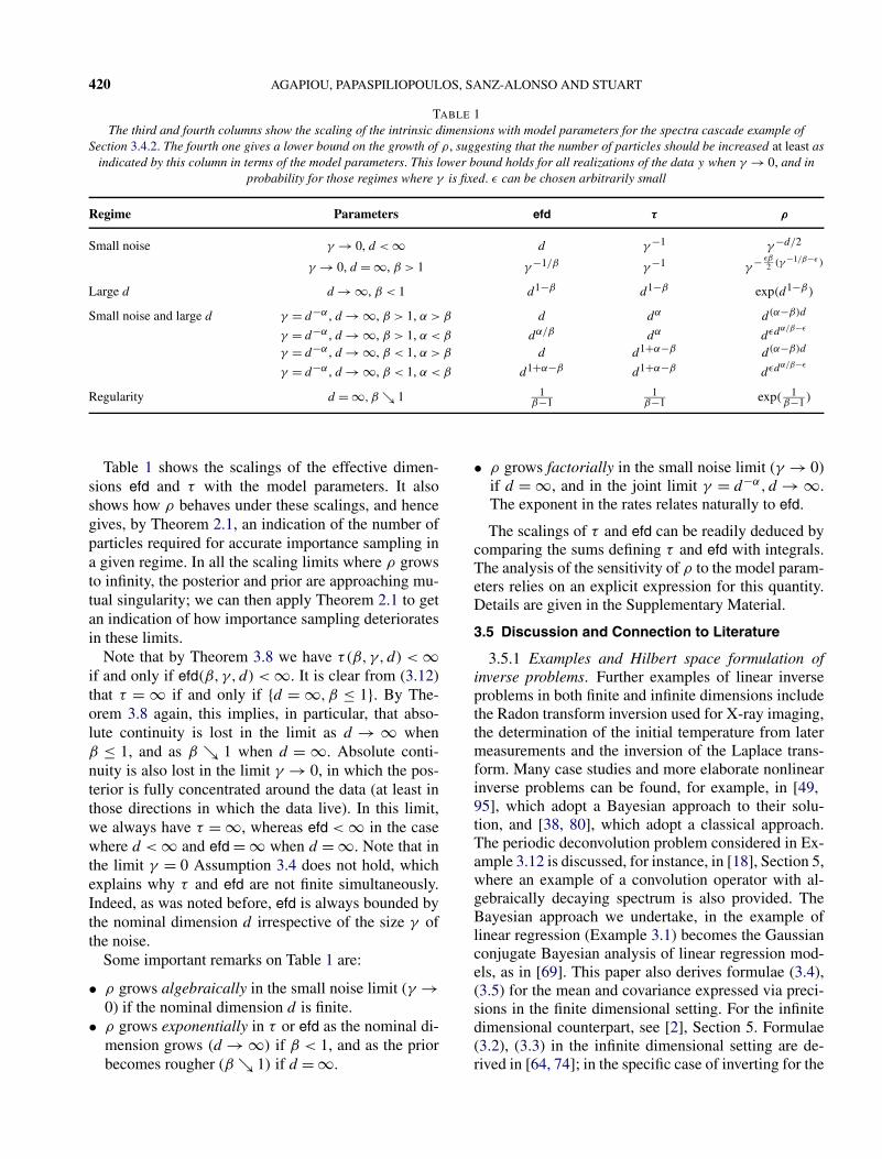
TABLE 1The third and fourth columns show the scaling of the intrinsic dimensions with model parameters for the spectra cascade example of
Section 3.4.2. The fourth one gives a lower bound on the growth of ρ, suggesting that the number of particles should be increased at least asindicated by this column in terms of the model parameters. This lower bound holds for all realizations of the data y when γ → 0, and in
probability for those regimes where γ is fixed. ε can be chosen arbitrarily small
Regime Parameters efd τ ρ
Small noise γ → 0, d < ∞ d γ −1 γ −d/2
γ → 0, d = ∞, β > 1 γ −1/β γ −1 γ − εβ2 (γ −1/β−ε )
Large d d → ∞, β < 1 d1−β d1−β exp(d1−β)
Small noise and large d γ = d−α , d → ∞, β > 1, α > β d dα d(α−β)d
γ = d−α , d → ∞, β > 1, α < β dα/β dα dεdα/β−ε
γ = d−α , d → ∞, β < 1, α > β d d1+α−β d(α−β)d
γ = d−α , d → ∞, β < 1, α < β d1+α−β d1+α−β dεdα/β−ε
Regularity d = ∞, β ↘ 1 1β−1
1β−1 exp( 1
β−1 )
Table 1 shows the scalings of the effective dimen-sions efd and τ with the model parameters. It alsoshows how ρ behaves under these scalings, and hencegives, by Theorem 2.1, an indication of the number ofparticles required for accurate importance sampling ina given regime. In all the scaling limits where ρ growsto infinity, the posterior and prior are approaching mu-tual singularity; we can then apply Theorem 2.1 to getan indication of how importance sampling deterioratesin these limits.
Note that by Theorem 3.8 we have τ(β, γ, d) < ∞if and only if efd(β, γ, d) < ∞. It is clear from (3.12)that τ = ∞ if and only if {d = ∞, β ≤ 1}. By The-orem 3.8 again, this implies, in particular, that abso-lute continuity is lost in the limit as d → ∞ whenβ ≤ 1, and as β ↘ 1 when d = ∞. Absolute conti-nuity is also lost in the limit γ → 0, in which the pos-terior is fully concentrated around the data (at least inthose directions in which the data live). In this limit,we always have τ = ∞, whereas efd < ∞ in the casewhere d < ∞ and efd = ∞ when d = ∞. Note that inthe limit γ = 0 Assumption 3.4 does not hold, whichexplains why τ and efd are not finite simultaneously.Indeed, as was noted before, efd is always bounded bythe nominal dimension d irrespective of the size γ ofthe noise.
Some important remarks on Table 1 are:
• ρ grows algebraically in the small noise limit (γ →0) if the nominal dimension d is finite.
• ρ grows exponentially in τ or efd as the nominal di-mension grows (d → ∞) if β < 1, and as the priorbecomes rougher (β ↘ 1) if d = ∞.
• ρ grows factorially in the small noise limit (γ → 0)if d = ∞, and in the joint limit γ = d−α, d → ∞.The exponent in the rates relates naturally to efd.
The scalings of τ and efd can be readily deduced bycomparing the sums defining τ and efd with integrals.The analysis of the sensitivity of ρ to the model param-eters relies on an explicit expression for this quantity.Details are given in the Supplementary Material.
3.5 Discussion and Connection to Literature
3.5.1 Examples and Hilbert space formulation ofinverse problems. Further examples of linear inverseproblems in both finite and infinite dimensions includethe Radon transform inversion used for X-ray imaging,the determination of the initial temperature from latermeasurements and the inversion of the Laplace trans-form. Many case studies and more elaborate nonlinearinverse problems can be found, for example, in [49,95], which adopt a Bayesian approach to their solu-tion, and [38, 80], which adopt a classical approach.The periodic deconvolution problem considered in Ex-ample 3.12 is discussed, for instance, in [18], Section 5,where an example of a convolution operator with al-gebraically decaying spectrum is also provided. TheBayesian approach we undertake, in the example oflinear regression (Example 3.1) becomes the Gaussianconjugate Bayesian analysis of linear regression mod-els, as in [69]. This paper also derives formulae (3.4),(3.5) for the mean and covariance expressed via preci-sions in the finite dimensional setting. For the infinitedimensional counterpart, see [2], Section 5. Formulae(3.2), (3.3) in the infinite dimensional setting are de-rived in [64, 74]; in the specific case of inverting for the
IMPORTANCE SAMPLING 421
initial condition in the heat equation they were derivedin [39]. The Supplementary Material has a discussionof Gaussian measures in Hilbert spaces and containsfurther background references.
3.5.2 The operator A: Centrality and assumptions.The assumption that the spectrum of A introducedin Assumption 3.4 consists of a countable number ofeigenvalues, means that the operator A can be thoughtof as an infinitely large diagonal matrix. It holds if A
is compact [63], Theorem 3, Chapter 28, but is in factmore general since it covers, for example, the noncom-pact case A = I .
We note here that the inverse problem
(3.13) y0 = w0 + η0
with η0 a white noise and w0 ∼ N(0, SS∗) is equiv-alent to (3.6), but formulated in terms of unknownw0 = Au0, rather than unknown u0. In this picture,the key operator is SS∗ rather than A = S∗S. Notethat by Lemma S.M.1.5 in the Supplementary MaterialTr(S∗S) = Tr(SS∗). Furthermore, if S is compact theoperators SS∗ and S∗S have the same nonzero eigen-values [38], Section 2.2, thus Tr((I + SS∗)−1SS∗) =Tr((I + S∗S)−1S∗S). The last equality holds even ifS is noncompact, since then Lemma S.M.1.5 togetherwith Lemma 3.7 imply that both sides are infinite.Combining, we see that the intrinsic dimension (τ orefd) is the same regardless of whether we view w0 oru0 as the unknown. In particular, the assumption thatA is bounded is equivalent to assuming that the op-erators S,S∗ or SS∗ are bounded [63], Theorem 14,Chapter 19. For the equivalent formulation (3.13), theposterior mean equation (3.2) is
m = SS∗(SS∗ + I
)−1y.
If SS∗ is compact, that is, if its nonzero eigenvaluesλi go to 0, then m is a regularized approximation ofw0, since the components of the data corresponding tosmall eigenvalues λi are shrunk towards zero. On theother hand, if SS∗ is unbounded, that is, if its nonzeroeigenvalues λi go to infinity, then there is no regular-ization and high frequency components in the data re-main almost unaffected by SS∗ in m. Therefore, thecase SS∗ is bounded is the borderline case determin-ing whether the prior has a regularizing effect in theinversion of the data.
The operator A has played an important role in thestudy of linear inverse problems. First, it has been usedfor obtaining posterior contraction rates in the smallnoise limit; see the operator B∗B in [3, 68]. Its usewas motivated by techniques for analyzing classical
regularization methods, in particular regularization inHilbert scales; see [38], Chapter 8. Furthermore, itseigenvalues and eigendirections can be used to deter-mine (optimal) low-rank approximations of the poste-rior covariance [15], [92], Theorem 2.3. The analogueof A in nonlinear Bayesian inverse problems is the so-called prior-preconditioned data-misfit Hessian, whichhas been used in [75] to design Metropolis–Hastingsproposals. In more realistic settings, the spectrum ofA may not be analytically available and needs to benumerically approximated; for example, see [15], Sec-tion 6.7, in the context of linearized global seismic in-version.
3.5.3 Notions of dimension and interpretations. InSection 3.2, we study notions of dimension forBayesian inverse problems. In the Bayesian setting, theprior imparts information and correlations on the com-ponents of the unknown u, reducing the number of pa-rameters that are estimated. In the context of Bayesianor penalized likelihood frameworks, this has led to thenotion of effective number of parameters, defined as
Tr(�1/2S
(I + S∗S
)−1S∗�−1/2)
.
This quantity agrees with efd by Proposition 3.6 andhas been used extensively in statistics and machinelearning; see, for example, the deviance informationcriterion in [93] (which generalises this notion tomore general Bayesian hierarchical models), and Sec-tion 3.5.3 of [12] and references therein. One motiva-tion for this definition is based on a Bayesian version ofthe “hat matrix”; see, for example, [93]. In this article,we provide a different motivation that is more relevantto our aims: rather than as an effective number of pa-rameters, we interpret efd as the effective dimensionof the Bayesian linear model. Similar forms of effec-tive dimension have been used for learning problemsin [17, 102, 103] and for statistical inverse problemsin [73]. In all of these contexts, the size of the oper-ator A quantifies how informative the data is; see thediscussion below. The paper [11] introduced the no-tion of τ = Tr(A) as an effective dimension for im-portance sampling within linear inverse problems andfiltering. In that paper, several transformations of theinverse problem are performed before doing the analy-sis. We undo these transformations here. The role of τ
in the performance of the ensemble Kalman filter hadbeen previously studied in [41].
Proposition 3.6 shows that efd is at most as large asthe nominal dimension. The difference between both isa measure of the effect the prior has on the inferencerelative to the maximum likelihood solution. Proposi-tion 3.5 shows that efd quantifies how far the poste-
422 AGAPIOU, PAPASPILIOPOULOS, SANZ-ALONSO AND STUART
rior is from the prior, measured in terms of how distanttheir covariances are in units of the prior; and similarlyfor τ , but expressed in terms of precisions and againin units of the prior. By the cyclic property of the trace,Lemma S.M.1.5(ii) in the Supplementary Material, andby Proposition 3.5, τ and efd may also be characterizedas follows:
τ = Tr((
C−1 − �−1)�
) = Tr((� − C)C−1)
,
efd = Tr((� − C)�−1) = Tr
((C−1 − �−1)
C).
Thus, we may also view efd as measuring the changein the precision, measured in units given by the pos-terior precision; whilst τ measures the change in thecovariance, measured in units given by the posteriorcovariance.
4. IMPORTANCE SAMPLING AND FILTERING
This section studies importance sampling in the con-text of filtering. In particular, we study two differentchoices of proposals that play an important role in thesubject of filtering. The analysis relies on the relation-ship between Bayesian inversion and filtering men-tioned in the introductory section, and detailed here.In Section 4.1, we set-up the problem and derive alink between importance sampling based particle fil-ters and the inverse problem. In Sections 4.2 and 4.3,we use this connection to study, respectively, the intrin-sic dimension of filtering and the connection to abso-lute continuity between the two proposals consideredand the target. Section 4.4 contains some explicit com-putations which enable comparison of the cost of thetwo proposals in various singular limits relating to highdimension or small observational noise. We concludewith the literature review Section 4.5.
The component of particle filtering which we anal-yse in this section is only that related to sequentialimportance sampling; we do not discuss the interac-tion between the simulated particles which arises viaresampling schemes. Such interaction would not typi-cally be very relevant in the two time-unit dynamicalsystems we study here, but would be necessary to getreasonable numerical schemes when assimilating dataover many time units. We comment further on this, andthe choice of the assimilation problem we study, in theliterature review.
4.1 General Setting
We simplify the notation by setting j = 0 in (1.3) toobtain
v1 = Mv0 + ξ, v0 ∼ N(0,P ), ξ ∼ N(0,Q),
y1 = Hv1 + ζ, ζ ∼ N(0,R).(4.1)
Note that we have also imposed a Gaussian assump-tion on v0. Because of the Markov assumption on thedynamics for {vj }, we have that v0 and ξ are inde-pendent. As in Section 3, we set-up the problem in aseparable Hilbert space H, although the reader versedonly in finite dimensional Gaussian measures shouldhave no trouble following the developments, simply bythinking of the covariance operators as (possibly infi-nite) matrices. We assume throughout that the covari-ance operators P,Q,R : H → H are bounded, self-adjoint, positive linear operators, but not necessarilytrace-class (see the discussion on this trace-class is-sue in Section 3). We also assume that the operatorsM,H : H → H that describe, respectively, the uncon-ditioned signal dynamics and the observation opera-tor, can be extended to larger spaces if necessary; seethe Supplementary Material for further details on thesetechnical issues.
Our goal in this section is to study the cost of impor-tance sampling within the context of both the standardand optimal proposals for particle filtering. For boththese proposals, we show that there is an inverse prob-lem embedded within the particle filtering method, andcompute the proposal covariance, the observation op-erator and the observational noise covariance. We maythen use the material from the previous section, con-cerning inverse problems, to make direct conclusionsabout the cost of importance sampling for particle fil-ters.
The aim of one step of filtering may be expressedas sampling from the target Pv1,v0|y1 . Particle filters dothis by importance sampling, with this measure on theproduct space X ×X as the target. We wish to comparetwo ways of doing this, one by using the proposal dis-tribution Pv1|v0Pv0 and the second by using as proposaldistribution Pv1|v0,y1Pv0 . The first is known as the stan-dard proposal, and the second as the optimal proposal.We now connect each of these proposals to a differentinverse problem.
4.1.1 Standard proposal. For the standard proposal,we note that, using Bayes’ theorem, conditioning, andthat the observation y1 does not depend on v0 explic-itly,
Pv1,v0|y1 ∝ Py1|v1,v0Pv1,v0
= Py1|v1,v0Pv1|v0Pv0
= Py1|v1Pv1|v0Pv0 .
Thus, the density of the target Pv1,v0|y1 with respectto the proposal Pv1|v0Pv0 is proportional to Py1|v1 . Al-though this density concerns a proposal on the joint
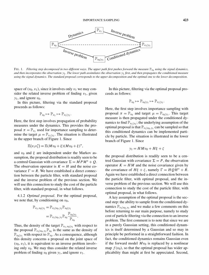
IMPORTANCE SAMPLING 423
Pv1
Pv0 Pv1|y1
Pv0|y1
Dynamics
Inverse problem
Inverse problem
Conditioned dynamics
FIG. 1. Filtering step decomposed in two different ways. The upper path first pushes forward the measure Pv0 using the signal dynamics,and then incorporates the observation y1. The lower path assimilates the observation y1 first, and then propagates the conditioned measureusing the signal dynamics. The standard proposal corresponds to the upper decomposition and the optimal one to the lower decomposition.
space of (v0, v1), since it involves only v1 we may con-sider the related inverse problem of finding v1, giveny1, and ignore v0.
In this picture, filtering via the standard proposalproceeds as follows:
Pv0 �→ Pv1 �→ Pv1|y1 .
Here, the first step involves propagation of probabilitymeasures under the dynamics. This provides the pro-posal π = Pv1 used for importance sampling to deter-mine the target μ = Pv1|y1 . The situation is illustratedin the upper branch of Figure 1. Since
E(v1v
∗1) = E(Mv0 + ξ)(Mv0 + ξ)∗,
and v0 and ξ are independent under the Markov as-sumption, the proposal distribution is readily seen to bea centred Gaussian with covariance � = MPM∗ + Q.The observation operator is K = H and the noise co-variance � = R. We have established a direct connec-tion between the particle filter, with standard proposaland the inverse problem of the previous section. Wewill use this connection to study the cost of the particlefilter, with standard proposal, in what follows.
4.1.2 Optimal proposal. For the optimal proposal,we note that, by conditioning on v0,
Pv1,v0|y1 = Pv1|v0,y1Pv0|y1
= Pv1|v0,y1Pv0
Pv0|y1
Pv0
.
Thus, the density of the target Pv1,v0|y1 with respect tothe proposal Pv1|v0,y1Pv0 is the same as the density ofPv0|y1 with respect to Pv0 . As a consequence, althoughthis density concerns a proposal on the joint space of(v0, v1), it is equivalent to an inverse problem involv-ing only v0. We may thus consider the related inverseproblem of finding v0 given y1, and ignore v1.
In this picture, filtering via the optimal proposal pro-ceeds as follows:
Pv0 �→ Pv0|y1 �→ Pv1|y1 .
Here, the first step involves importance sampling withproposal π = Pv0 and target μ = Pv0|y1 . This targetmeasure is then propagated under the conditioned dy-namics to find Pv1|y1 ; the underlying assumption of theoptimal proposal is that Pv1|v0,y1 can be sampled so thatthis conditioned dynamics can be implemented parti-cle by particle. The situation is illustrated in the lowerbranch of Figure 1. Since
y1 = HMv0 + Hξ + ζ
the proposal distribution is readily seen to be a cen-tred Gaussian with covariance � = P , the observationoperator K = HM and the noise covariance given bythe covariance of Hξ + ζ , namely � = HQH ∗ + R.Again we have established a direct connection betweenthe particle filter, with optimal proposal, and the in-verse problem of the previous section. We will use thisconnection to study the cost of the particle filter, withoptimal proposal, in what follows.
A key assumption of the optimal proposal is the sec-ond step: the ability to sample from the conditioned dy-namics Pv1|v0,y1 and we make a few comments on thisbefore returning to our main purpose, namely to studycost of particle filtering via the connection to an inverseproblem. The first comment is to note that since we arein a purely Gaussian setting, this conditioned dynam-ics is itself determined by a Gaussian and so may inprinciple be performed in a straightforward fashion. Infact, the conditioned dynamics remains Gaussian evenif the forward model Mv0 is replaced by a nonlinearmap f (v0), so that the optimal proposal has wider ap-plicability than might at first be appreciated. Second,

424 AGAPIOU, PAPASPILIOPOULOS, SANZ-ALONSO AND STUART
TABLE 2Comparison of the standard and optimal proposals
Standard proposal Optimal proposal
Proposal Pv0(dv0)Pv1|v0(dv1) Pv0(dv0)Pv1|v0,y1 (dv1)
BIP y1 = Hv1 + ηst y1 = HMv0 + ηopPrior Cov. MPM∗ + Q P
Data Cov. R R + HQH∗logg(u;y1) − 1
2‖Hv1‖2R + 〈y1,Hv1〉R − 1
2‖HMv0‖2R+HQH ∗ + 〈y1,HMv0〉R+HQH ∗
we comment that the Gaussian arising in the condi-tioned dynamics has mean m and variance � given bythe formulae
� = Q − QH ∗(HQH ∗ + R
)−1HQ,
m = Mv0 + QH ∗(HQH ∗ + R
)−1(y1 − HMv0).
It is a tacit assumption in what follows that the op-erators defining the filtering problem are such that� : H → H is well-defined and that m ∈ H is well-defined. More can be said about these points, but doingso will add further technicalities without contributingto the main goals of this paper.
4.2 Intrinsic Dimension
Using the inverse problems that arise for the standardproposal and for the optimal proposal, and employingthem within the definition of A from Assumption 3.4,we find the two operators A arising for these two dif-ferent proposals:
A := Ast
:= (MPM∗ + Q
)1/2H ∗R−1H
(MPM∗ + Q
)1/2
for the standard proposal, and
A := Aop := P12 M∗H ∗(
R + HQH ∗)−1HMP 1/2
for the optimal proposal. Again here it is assumed thatthese operators are bounded in H:
ASSUMPTION 4.1. The operators Ast and Aop,viewed as linear operators in H, are bounded. Fur-thermore, the spectra of both Ast and Aop consist ofa countable number of eigenvalues.
Using these definitions of Ast and Aop, we may de-fine, from (3.7), the intrinsic dimensions τst, efdst forthe standard proposal and τop, efdop for the optimal onein the following way:
τst = Tr(Ast), efdst = Tr((I + Ast)
−1Ast)
and
τop = Tr(Aop), efdop = Tr((I + Aop)
−1Aop).
4.3 Absolute Continuity
The following two theorems are a straightforwardapplication of Theorem 3.8, using the connections be-tween filtering and inverse problems made above. Thecontents of the two theorems are summarized in Ta-ble 2.
THEOREM 4.2. Consider one-step of particle fil-tering for (4.1). Let μ = Pv1|y1 and π = Pv1 = N(0,
Q + MPM∗). Then the following are equivalent:
(i) efdst < ∞;(ii) τst < ∞;
(iii) R−1/2Hv1 ∈H, π -almost surely;(iv) for νy -almost all y, the target distribution μ is
well-defined as a measure in X and is absolutelycontinuous with respect to the proposal with
(4.2)
dμ
dπ(v1)
∝ exp(−1
2
∥∥R−1/2Hv1∥∥2
+ 1
2
⟨R−1/2y1,R
−1/2Hv1⟩)
=: gst(v1;y1),
where 0 < π(gst(·;y1)) < ∞.
THEOREM 4.3. Consider one-step of particle fil-tering for (4.1). Let μ = Pv0|y1 and π = Pv0 = N(0,
Q). Then, for Rop = R + HQH ∗, the following areequivalent:
(i) efdop < ∞;(ii) τop < ∞;
(iii) R−1/2op HMv0 ∈ H, π -almost surely;
(iv) for νy -almost all y, the target distribution μ iswell defined as a measure in X and is absolutely
IMPORTANCE SAMPLING 425
continuous with respect to the proposal with
(4.3)
dμ
dπ(v0)
∝ exp(−1
2
∥∥R−1/2op HMv0
∥∥2
+ 1
2
⟨R−1/2
op y1,R−1/2op HMv0
⟩)
=: gop(v0;y1),
where 0 < π(gop(·;y1)) < ∞.
REMARK 4.4. Because of the exponential struc-ture of gst and gop, the assertion (iv) in the preced-ing two theorems is equivalent to gst and gop beingν-almost surely positive and finite and for almost ally1 the second moment of the target-proposal densitybeing finite. This second moment is given, for the stan-dard and optimal proposals, by
ρst = π(gst(·;y)2)
π(gst(·;y))2 < ∞and
ρop = π(gop(·;y)2)
π(gop(·;y))2 < ∞
respectively. The relative sizes of ρst and ρop determinethe relative efficiency of the standard and optimal pro-posal versions of filtering.
The following theorem shows that there is loss ofabsolute continuity for the standard proposal wheneverthere is for the optimal one. The result is formulated interms of the intrinsic dimension τ , and we show thatτop = ∞ implies τst = ∞; by Theorem 3.8, this im-plies the result concerning absolute continuity. Recall-ing that poor behaviour of importance sampling is inti-mately related to such breakdown, this suggests that theoptimal proposal is always at least as good as the stan-dard one. The following theorem also gives a condi-tion on the operators H , Q and R under which collapsefor both proposals occurs at the same time, irrespectiveof the regularity of the operators M and P . Roughlyspeaking, this simultaneous collapse result states thatif R is large compared to Q then absolute continuityfor both proposals is equivalent; and hence collapseof importance sampling happens under one proposalif and only if it happens under the other. Intuitively,the advantages of the optimal proposal stem from thenoise in the dynamics; they disappear completely if thedynamics is deterministic. The theorem quantifies thisidea. Finally, an example demonstrates that there are
situations where τop is finite, so that optimal proposalbased importance sampling works well for finite di-mensional approximations of an infinite dimensionalproblem, whilst τst is infinite, so that standard proposalbased importance sampling works poorly for finite di-mensional approximations.
THEOREM 4.5. Suppose that Assumption 4.1holds. Then
(4.4) τop ≤ τst.
Moreover, if Tr(HQH ∗R−1) < ∞, then
τst < ∞ ⇐⇒ τop < ∞.
We remark that, under additional simplifying as-sumptions, we can obtain bounds of the form (4.4) forefd and ρ. We chose to formulate the result in terms ofτ since we can prove the bound (4.4) in full general-ity. Moreover, by Theorem 3.8 the bound in terms ofτ suffices in order to understand the different collapseproperties of both proposals.
The following example demonstrates that it is possi-ble that τop < ∞ while τst = ∞; in this situation, fil-tering via the optimal proposal is well-defined, whilstusing the standard proposal it is not. Loosely speak-ing, this happens if y1 provides more information onv1 than v0.
EXAMPLE 4.6. Suppose that
H = Q = R = M = I, Tr(P ) < ∞.
Then it is straightforward from the definitions thatAst = P + I and Aop = P/2. In an infinite dimensionalHilbert space setting, the identity operator has infinitetrace, Tr(I ) = ∞, and so
τst = Tr(Ast) = Tr(P + I ) = ∞,
τop = Tr(Aop) = Tr(P/2) < ∞.
We have thus established an example of a filteringmodel for which τst = ∞ and τop < ∞. We note thatby Theorem 4.5, any such example satisfies the condi-tion Tr(HQH ∗R−1) = ∞. When this condition is met,automatically τst = ∞. However, τop can still be finite.Indeed, within the proof of that theorem in the Supple-mentary Material we show that the inequality
τop ≤ Tr(R−1HMPM∗H ∗)
always holds. The right-hand side may be finite pro-vided that the eigenvalues of P decay fast enough.A simple example of this situation is where HM is abounded operator and all the relevant operators have
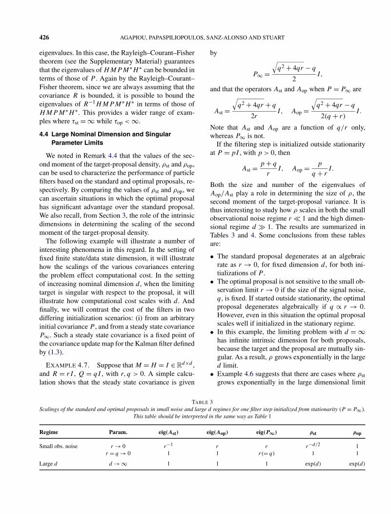
426 AGAPIOU, PAPASPILIOPOULOS, SANZ-ALONSO AND STUART
eigenvalues. In this case, the Rayleigh–Courant–Fishertheorem (see the Supplementary Material) guaranteesthat the eigenvalues of HMPM∗H ∗ can be bounded interms of those of P . Again by the Rayleigh–Courant–Fisher theorem, since we are always assuming that thecovariance R is bounded, it is possible to bound theeigenvalues of R−1HMPM∗H ∗ in terms of those ofHMPM∗H ∗. This provides a wider range of exam-ples where τst = ∞ while τop < ∞.
4.4 Large Nominal Dimension and SingularParameter Limits
We noted in Remark 4.4 that the values of the sec-ond moment of the target-proposal density, ρst and ρop,can be used to characterize the performance of particlefilters based on the standard and optimal proposals, re-spectively. By comparing the values of ρst and ρop, wecan ascertain situations in which the optimal proposalhas significant advantage over the standard proposal.We also recall, from Section 3, the role of the intrinsicdimensions in determining the scaling of the secondmoment of the target-proposal density.
The following example will illustrate a number ofinteresting phenomena in this regard. In the setting offixed finite state/data state dimension, it will illustratehow the scalings of the various covariances enteringthe problem effect computational cost. In the settingof increasing nominal dimension d , when the limitingtarget is singular with respect to the proposal, it willillustrate how computational cost scales with d . Andfinally, we will contrast the cost of the filters in twodiffering initialization scenarios: (i) from an arbitraryinitial covariance P , and from a steady state covarianceP∞. Such a steady state covariance is a fixed point ofthe covariance update map for the Kalman filter definedby (1.3).
EXAMPLE 4.7. Suppose that M = H = I ∈ Rd×d ,
and R = rI , Q = qI , with r, q > 0. A simple calcu-lation shows that the steady state covariance is given
by
P∞ =√
q2 + 4qr − q
2I,
and that the operators Ast and Aop when P = P∞ are
Ast =√
q2 + 4qr + q
2rI, Aop =
√q2 + 4qr − q
2(q + r)I.
Note that Ast and Aop are a function of q/r only,whereas P∞ is not.
If the filtering step is initialized outside stationarityat P = pI , with p > 0, then
Ast = p + q
rI, Aop = p
q + rI.
Both the size and number of the eigenvalues ofAop/Ast play a role in determining the size of ρ, thesecond moment of the target-proposal variance. It isthus interesting to study how ρ scales in both the smallobservational noise regime r � 1 and the high dimen-sional regime d � 1. The results are summarized inTables 3 and 4. Some conclusions from these tablesare:
• The standard proposal degenerates at an algebraicrate as r → 0, for fixed dimension d , for both ini-tializations of P .
• The optimal proposal is not sensitive to the small ob-servation limit r → 0 if the size of the signal noise,q , is fixed. If started outside stationarity, the optimalproposal degenerates algebraically if q ∝ r → 0.However, even in this situation the optimal proposalscales well if initialized in the stationary regime.
• In this example, the limiting problem with d = ∞has infinite intrinsic dimension for both proposals,because the target and the proposal are mutually sin-gular. As a result, ρ grows exponentially in the larged limit.
• Example 4.6 suggests that there are cases where ρstgrows exponentially in the large dimensional limit
TABLE 3Scalings of the standard and optimal proposals in small noise and large d regimes for one filter step initialized from stationarity (P = P∞).
This table should be interpreted in the same way as Table 1
Regime Param. eig(Ast) eig(Aop) eig(P∞) ρst ρop
Small obs. noise r → 0 r−1 r r r−d/2 1r = q → 0 1 1 r(= q) 1 1
Large d d → ∞ 1 1 1 exp(d) exp(d)
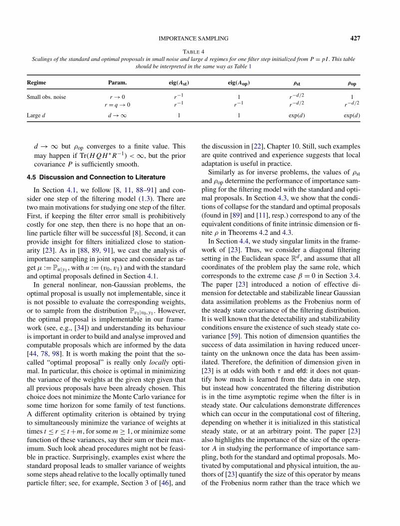
IMPORTANCE SAMPLING 427
TABLE 4Scalings of the standard and optimal proposals in small noise and large d regimes for one filter step initialized from P = pI . This table
should be interpreted in the same way as Table 1
Regime Param. eig(Ast) eig(Aop) ρst ρop
Small obs. noise r → 0 r−1 1 r−d/2 1r = q → 0 r−1 r−1 r−d/2 r−d/2
Large d d → ∞ 1 1 exp(d) exp(d)
d → ∞ but ρop converges to a finite value. Thismay happen if Tr(HQH ∗R−1) < ∞, but the priorcovariance P is sufficiently smooth.
4.5 Discussion and Connection to Literature
In Section 4.1, we follow [8, 11, 88–91] and con-sider one step of the filtering model (1.3). There aretwo main motivations for studying one step of the filter.First, if keeping the filter error small is prohibitivelycostly for one step, then there is no hope that an on-line particle filter will be successful [8]. Second, it canprovide insight for filters initialized close to station-arity [23]. As in [88, 89, 91], we cast the analysis ofimportance sampling in joint space and consider as tar-get μ := Pu|y1 , with u := (v0, v1) and with the standardand optimal proposals defined in Section 4.1.
In general nonlinear, non-Gaussian problems, theoptimal proposal is usually not implementable, since itis not possible to evaluate the corresponding weights,or to sample from the distribution Pv1|v0,y1 . However,the optimal proposal is implementable in our frame-work (see, e.g., [34]) and understanding its behaviouris important in order to build and analyse improved andcomputable proposals which are informed by the data[44, 78, 98]. It is worth making the point that the so-called “optimal proposal” is really only locally opti-mal. In particular, this choice is optimal in minimizingthe variance of the weights at the given step given thatall previous proposals have been already chosen. Thischoice does not minimize the Monte Carlo variance forsome time horizon for some family of test functions.A different optimality criterion is obtained by tryingto simultaneously minimize the variance of weights attimes t ≤ r ≤ t +m, for some m ≥ 1, or minimize somefunction of these variances, say their sum or their max-imum. Such look ahead procedures might not be feasi-ble in practice. Surprisingly, examples exist where thestandard proposal leads to smaller variance of weightssome steps ahead relative to the locally optimally tunedparticle filter; see, for example, Section 3 of [46], and
the discussion in [22], Chapter 10. Still, such examplesare quite contrived and experience suggests that localadaptation is useful in practice.
Similarly as for inverse problems, the values of ρstand ρop determine the performance of importance sam-pling for the filtering model with the standard and opti-mal proposals. In Section 4.3, we show that the condi-tions of collapse for the standard and optimal proposals(found in [89] and [11], resp.) correspond to any of theequivalent conditions of finite intrinsic dimension or fi-nite ρ in Theorems 4.2 and 4.3.
In Section 4.4, we study singular limits in the frame-work of [23]. Thus, we consider a diagonal filteringsetting in the Euclidean space R
d , and assume that allcoordinates of the problem play the same role, whichcorresponds to the extreme case β = 0 in Section 3.4.The paper [23] introduced a notion of effective di-mension for detectable and stabilizable linear Gaussiandata assimilation problems as the Frobenius norm ofthe steady state covariance of the filtering distribution.It is well known that the detectability and stabilizabilityconditions ensure the existence of such steady state co-variance [59]. This notion of dimension quantifies thesuccess of data assimilation in having reduced uncer-tainty on the unknown once the data has been assim-ilated. Therefore, the definition of dimension given in[23] is at odds with both τ and efd: it does not quan-tify how much is learned from the data in one step,but instead how concentrated the filtering distributionis in the time asymptotic regime when the filter is insteady state. Our calculations demonstrate differenceswhich can occur in the computational cost of filtering,depending on whether it is initialized in this statisticalsteady state, or at an arbitrary point. The paper [23]also highlights the importance of the size of the opera-tor A in studying the performance of importance sam-pling, both for the standard and optimal proposals. Mo-tivated by computational and physical intuition, the au-thors of [23] quantify the size of this operator by meansof the Frobenius norm rather than the trace which we
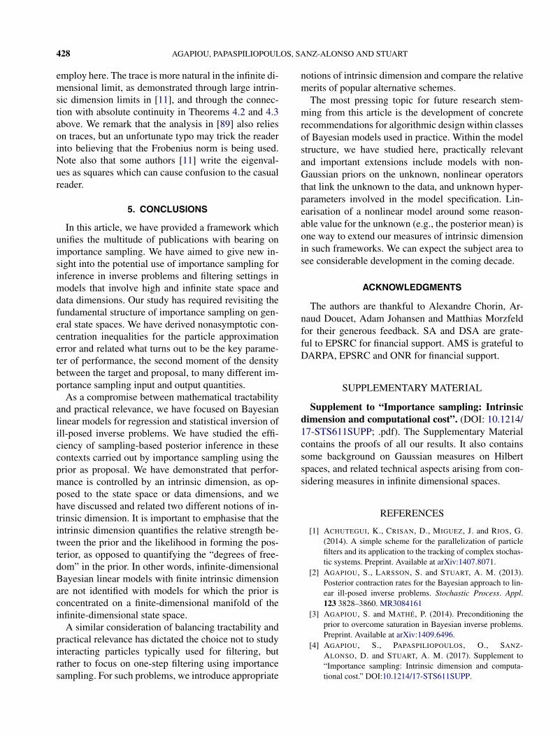
428 AGAPIOU, PAPASPILIOPOULOS, SANZ-ALONSO AND STUART
employ here. The trace is more natural in the infinite di-mensional limit, as demonstrated through large intrin-sic dimension limits in [11], and through the connec-tion with absolute continuity in Theorems 4.2 and 4.3above. We remark that the analysis in [89] also relieson traces, but an unfortunate typo may trick the readerinto believing that the Frobenius norm is being used.Note also that some authors [11] write the eigenval-ues as squares which can cause confusion to the casualreader.
5. CONCLUSIONS
In this article, we have provided a framework whichunifies the multitude of publications with bearing onimportance sampling. We have aimed to give new in-sight into the potential use of importance sampling forinference in inverse problems and filtering settings inmodels that involve high and infinite state space anddata dimensions. Our study has required revisiting thefundamental structure of importance sampling on gen-eral state spaces. We have derived nonasymptotic con-centration inequalities for the particle approximationerror and related what turns out to be the key parame-ter of performance, the second moment of the densitybetween the target and proposal, to many different im-portance sampling input and output quantities.
As a compromise between mathematical tractabilityand practical relevance, we have focused on Bayesianlinear models for regression and statistical inversion ofill-posed inverse problems. We have studied the effi-ciency of sampling-based posterior inference in thesecontexts carried out by importance sampling using theprior as proposal. We have demonstrated that perfor-mance is controlled by an intrinsic dimension, as op-posed to the state space or data dimensions, and wehave discussed and related two different notions of in-trinsic dimension. It is important to emphasise that theintrinsic dimension quantifies the relative strength be-tween the prior and the likelihood in forming the pos-terior, as opposed to quantifying the “degrees of free-dom” in the prior. In other words, infinite-dimensionalBayesian linear models with finite intrinsic dimensionare not identified with models for which the prior isconcentrated on a finite-dimensional manifold of theinfinite-dimensional state space.
A similar consideration of balancing tractability andpractical relevance has dictated the choice not to studyinteracting particles typically used for filtering, butrather to focus on one-step filtering using importancesampling. For such problems, we introduce appropriate
notions of intrinsic dimension and compare the relativemerits of popular alternative schemes.
The most pressing topic for future research stem-ming from this article is the development of concreterecommendations for algorithmic design within classesof Bayesian models used in practice. Within the modelstructure, we have studied here, practically relevantand important extensions include models with non-Gaussian priors on the unknown, nonlinear operatorsthat link the unknown to the data, and unknown hyper-parameters involved in the model specification. Lin-earisation of a nonlinear model around some reason-able value for the unknown (e.g., the posterior mean) isone way to extend our measures of intrinsic dimensionin such frameworks. We can expect the subject area tosee considerable development in the coming decade.
ACKNOWLEDGMENTS
The authors are thankful to Alexandre Chorin, Ar-naud Doucet, Adam Johansen and Matthias Morzfeldfor their generous feedback. SA and DSA are grate-ful to EPSRC for financial support. AMS is grateful toDARPA, EPSRC and ONR for financial support.
SUPPLEMENTARY MATERIAL
Supplement to “Importance sampling: Intrinsicdimension and computational cost”. (DOI: 10.1214/17-STS611SUPP; .pdf). The Supplementary Materialcontains the proofs of all our results. It also containssome background on Gaussian measures on Hilbertspaces, and related technical aspects arising from con-sidering measures in infinite dimensional spaces.
REFERENCES
[1] ACHUTEGUI, K., CRISAN, D., MIGUEZ, J. and RIOS, G.(2014). A simple scheme for the parallelization of particlefilters and its application to the tracking of complex stochas-tic systems. Preprint. Available at arXiv:1407.8071.
[2] AGAPIOU, S., LARSSON, S. and STUART, A. M. (2013).Posterior contraction rates for the Bayesian approach to lin-ear ill-posed inverse problems. Stochastic Process. Appl.123 3828–3860. MR3084161
[3] AGAPIOU, S. and MATHÉ, P. (2014). Preconditioning theprior to overcome saturation in Bayesian inverse problems.Preprint. Available at arXiv:1409.6496.
[4] AGAPIOU, S., PAPASPILIOPOULOS, O., SANZ-ALONSO, D. and STUART, A. M. (2017). Supplement to“Importance sampling: Intrinsic dimension and computa-tional cost.” DOI:10.1214/17-STS611SUPP.
IMPORTANCE SAMPLING 429
[5] AGAPIOU, S., STUART, A. M. and ZHANG, Y.-X. (2014).Bayesian posterior contraction rates for linear severely ill-posed inverse problems. J. Inverse Ill-Posed Probl. 22 297–321. MR3215928
[6] BAIN, A. and CRISAN, D. (2009). Fundamentals ofStochastic Filtering 3. Springer, Berlin.
[7] BENDER, C. M. and ORSZAG, S. A. (1999). AdvancedMathematical Methods for Scientists and Engineers. I.Asymptotic Methods and Perturbation Theory. Springer,New York. MR1721985
[8] BENGTSSON, T., BICKEL, P., LI, B. et al. (2008). Curse-of-dimensionality revisited: Collapse of the particle filter invery large scale systems. In Probability and Statistics: Es-says in Honor of David A. Freedman. Inst. Math. Stat. (IMS)Collect. 316–334. IMS, Beachwood, OH.
[9] BESKOS, A., CRISAN, D. and JASRA, A. (2014). On thestability of sequential Monte Carlo methods in high dimen-sions. Ann. Appl. Probab. 24 1396–1445. MR3211000
[10] BESKOS, A., CRISAN, D., JASRA, A., KAMATANI, K. andZHOU, Y. (2014). A stable particle filter in high-dimensions.Preprint. Available at 1412.3501.
[11] BICKEL, P., LI, B. and BENGTSSON, T. (2008). Sharp fail-ure rates for the bootstrap particle filter in high dimensions.In Pushing the Limits of Contemporary Statistics: Contribu-tions in Honor of Jayanta K. Ghosh. Inst. Math. Stat. (IMS)Collect. 3 318–329. IMS, Beachwood, OH. MR2459233
[12] BISHOP, C. M. (2006). Pattern Recognition and MachineLearning. Springer, New York. MR2247587
[13] BOUCHERON, S., LUGOSI, G. and MASSART, P. (2013).Concentration Inequalities. Oxford Univ. Press, Oxford.MR3185193
[14] BUI-THANH, T. and GHATTAS, O. (2012). Analysis of theHessian for inverse scattering problems: I. Inverse shapescattering of acoustic waves. Inverse Problems 28 055001,32. MR2915289
[15] BUI-THANH, T., GHATTAS, O., MARTIN, J. andSTADLER, G. (2013). A computational framework forinfinite-dimensional Bayesian inverse problems part I: Thelinearized case, with application to global seismic inversion.SIAM J. Sci. Comput. 35 A2494–A2523.
[16] CAFLISCH, R. E., MOROKOFF, W. J. and OWEN, A. B.(1997). Valuation of Mortgage Backed Securities UsingBrownian Bridges to Reduce Effective Dimension. Dept.Mathematics, Univ. California, Los Angeles.
[17] CAPONNETTO, A. and DE VITO, E. (2007). Optimal ratesfor the regularized least-squares algorithm. Found. Comput.Math. 7 331–368.
[18] CAVALIER, L. and TSYBAKOV, A. (2002). Sharp adaptationfor inverse problems with random noise. Probab. Theory Re-lated Fields 123 323–354.
[19] CHATTERJEE, S. and DIACONIS, P. (2015). The samplesize required in importance sampling. Preprint. Available atarXiv:1511.01437.
[20] CHEN, Y. (2005). Another look at rejection samplingthrough importance sampling. Statist. Probab. Lett. 72 277–283. MR2153124
[21] CHOPIN, N. (2004). Central limit theorem for sequentialMonte Carlo methods and its application to Bayesian infer-ence. Ann. Statist. 32 2385–2411. MR2153989
[22] CHOPIN, N. and PAPASPILIOPOULOS, O. (2016). A Con-cise Introduction to Sequential Monte Carlo.
[23] CHORIN, A. J. and MORZFELD, M. (2013). Conditionsfor successful data assimilation. Journal of Geophysical Re-search: Atmospheres 118 11–522.
[24] CONSTANTINE, P. G. (2015). Active Subspaces: Emerg-ing Ideas for Dimension Reduction in Parameter Studies 2.SIAM Spotlights, Philadelphia, PA.
[25] COTTER, S. L., ROBERTS, G. O., STUART, A. M. andWHITE, D. (2013). MCMC methods for functions: Mod-ifying old algorithms to make them faster. Statist. Sci. 28424–446. MR3135540
[26] CRISAN, D., DEL MORAL, P. and LYONS, T. (1999). Dis-crete filtering using branching and interacting particle sys-tems. Markov Process. Related Fields 5 293–318.
[27] CRISAN, D. and DOUCET, A. (2002). A survey of conver-gence results on particle filtering methods for practitioners.IEEE Trans. Signal Process. 50 736–746.
[28] CRISAN, D. and ROZOVSKII, B., eds. (2011). The OxfordHandbook of Nonlinear Filtering. Oxford Univ. Press, Ox-ford. MR2882749
[29] CUI, T., MARTIN, J., MARZOUK, Y. M., SOLONEN, A.and SPANTINI, A. (2014). Likelihood-informed dimensionreduction for nonlinear inverse problems. Inverse Problems30 114015, 28. MR3274599
[30] DASHTI, M. and STUART, A. M. (2016). The Bayesian ap-proach to inverse problems. In Handbook of UncertaintyQuantification (R. Ghanem, D. Higdon and H. Owhadi,eds.). http://arxiv.org/abs/1302.6989.
[31] DEL MORAL, P. (2004). Feynman–Kac Formulae. Springer,New York. MR2044973
[32] DEL MORAL, P. and MICLO, L. (2000). Branching and in-teracting particle systems approximations of Feynman–Kacformulae with applications to non-linear filtering. In Sémi-naire de Probabilités, XXXIV. Lecture Notes in Math. 17291–145. Springer, Berlin. MR1768060
[33] DOUCET, A., DE FREITAS, N. and GORDON, N. (2001).An introduction to sequential Monte Carlo methods. In Se-quential Monte Carlo Methods in Practice. 3–14. Springer,New York. MR1847784
[34] DOUCET, A., GODSILL, S. and ANDRIEU, C. (2000). Onsequential Monte Carlo sampling methods for Bayesian fil-tering. Stat. Comput. 10 197–208.
[35] DOUKHAN, P. and LANG, G. (2009). Evaluation for mo-ments of a ratio with application to regression estimation.Bernoulli 15 1259–1286.
[36] DOWNEY, P. J. and WRIGHT, P. E. (2007). The ratio of theextreme to the sum in a random sequence. Extremes 10 249–266.
[37] DUPUIS, P., SPILIOPOULOS, K. and WANG, H. (2012).Importance sampling for multiscale diffusions. MultiscaleModel. Simul. 10 1–27. MR2902596
[38] ENGL, H. W., HANKE, M. and NEUBAUER, A.(1996). Regularization of Inverse Problems. Mathematicsand Its Applications 375. Kluwer Academic, Dordrecht.MR1408680
[39] FRANKLIN, J. N. (1970). Well-posed stochastic extensionsof ill-posed linear problems. J. Math. Anal. Appl. 31 682–716. MR0267654

430 AGAPIOU, PAPASPILIOPOULOS, SANZ-ALONSO AND STUART
[40] FREI, M. and KÜNSCH, H. R. (2013). Bridging the ensem-ble Kalman and particle filters. Biometrika 100 781–800.
[41] FURRER, R. and BENGTSSON, T. (2007). Estimation ofhigh-dimensional prior and posterior covariance matrices inKalman filter variants. J. Multivariate Anal. 98 227–255.
[42] GELMAN, A., ROBERTS, G. O. and GILKS, W. R. (1996).Efficient Metropolis jumping rules. In Bayesian Statistics, 5(Alicante, 1994). 599–607. Oxford Univ. Press, New York.MR1425429
[43] GIBBS, A. L. and SU, F. E. (2002). On choosing andbounding probability metrics. Int. Stat. Rev. 70 419–435.
[44] GOODMAN, J., LIN, K. K. and MORZFELD, M. (2015).Small-noise analysis and symmetrization of implicit MonteCarlo samplers. Comm. Pure Appl. Math.
[45] HAN, W. (2013). On the Numerical Solution of the FilteringProblem Ph.D. thesis, Dept. Mathematics, Imperial College,London.
[46] JOHANSEN, A. M. and DOUCET, A. (2008). A note on aux-iliary particle filters. Statist. Probab. Lett. 78 1498–1504.
[47] KAHN, H. (1955). Use of Different Monte Carlo SamplingTechniques. Rand Corporation, Santa Monica, CA.
[48] KAHN, H. and MARSHALL, A. W. (1953). Methods of re-ducing sample size in Monte Carlo computations. Journal ofthe Operations Research Society of America 1 263–278.
[49] KAIPIO, J. and SOMERSALO, E. (2005). Statistical andComputational Inverse Problems. Applied MathematicalSciences 160. Springer, New York. MR2102218
[50] KALLENBERG, O. (2002). Foundations of Modern Prob-ability. Probability and Its Applications, 2nd ed. Springer,Berlin.
[51] KALMAN, R. E. (1960). A new approach to linear filteringand prediction problems. J. Fluids Eng. 82 35–45.
[52] KALNAY, E. (2003). Atmospheric Modeling, Data Assimila-tion, and Predictability. Cambridge Univ. Press, Cambridge.
[53] KEKKONEN, H., LASSAS, M. and SILTANEN, S. (2016).Posterior consistency and convergence rates for Bayesianinversion with hypoelliptic operators. Inverse Probl. 32085005, 31. MR3535664
[54] KNAPIK, B. T., VAN DER VAART, A. W. and VAN ZAN-TEN, J. H. (2011). Bayesian inverse problems with Gaussianpriors. Ann. Statist. 39 2626–2657.
[55] KNAPIK, B. T., VAN DER VAART, A. W. and VAN ZAN-TEN, J. H. (2013). Bayesian recovery of the initial condi-tion for the heat equation. Comm. Statist. Theory Methods42 1294–1313.
[56] KONG, A. (1992). A note on importance sampling usingstandardized weights. Technical Report 348, Dept. Statis-tics, Univ. Chicago, Chicago, IL.
[57] KONG, A., LIU, J. S. and WONG, W. H. (1994). Sequentialimputations and Bayesian missing data problems. J. Amer.Statist. Assoc. 89 278–288.
[58] KUO, F. Y. and SLOAN, I. H. (2005). Lifting the curseof dimensionality. Notices Amer. Math. Soc. 52 1320–1329.MR2183869
[59] LANCASTER, P. and RODMAN, L. (1995). Algebraic Ric-cati Equations. Oxford Univ. Press, London.
[60] LASANEN, S. (2007). Measurements and infinite-dimensional statistical inverse theory. PAMM 7 1080101–1080102.
[61] LASANEN, S. (2012). Non-Gaussian statistical inverseproblems. Part I: Posterior distributions. Inverse Probl.Imaging 6 215–266. MR2942739
[62] LASANEN, S. (2012). Non-Gaussian statistical inverseproblems. Part II: Posterior convergence for approximatedunknowns. Inverse Probl. Imaging 6 267–287.
[63] LAX, P. D. (2002). Functional Analysis. Wiley, New York.[64] LEHTINEN, M. S., PAIVARINTA, L. and SOMERSALO, E.
(1989). Linear inverse problems for generalised randomvariables. Inverse Probl. 5 599.
[65] LE GLAND, F., MONBET, V. and TRAN, V. (2009). Largesample asymptotics for the ensemble Kalman filter Ph.D.thesis, INRIA.
[66] LI, W., TAN, Z. and CHEN, R. (2013). Two-stage impor-tance sampling with mixture proposals. J. Amer. Statist. As-soc. 108 1350–1365.
[67] LIANG, F., LIU, C. and CARROLL, R. J. (2007). Stochasticapproximation in Monte Carlo computation. J. Amer. Statist.Assoc. 102 305–320.
[68] LIN, K., LU, S. and MATHÉ, P. (2015). Oracle-type poste-rior contraction rates in Bayesian inverse problems. InverseProbl. Imaging 9.
[69] LINDLEY, D. V. and SMITH, A. F. M. (1972). Bayes es-timates for the linear model. J. R. Stat. Soc. Ser. B. Stat.Methodol. 34 1–41. MR0415861
[70] LIU, J. S. (1996). Metropolized independent sampling withcomparisons to rejection sampling and importance sam-pling. Stat. Comput. 6 113–119.
[71] LIU, J. S. (2008). Monte Carlo Strategies in Scientific Com-puting. Springer, New York. MR2401592
[72] LIU, J. S. and CHEN, R. (1998). Sequential Monte Carlomethods for dynamic systems. J. Amer. Statist. Assoc. 931032–1044. MR1649198
[73] LU, S. and MATHÉ, P. (2014). Discrepancy based model se-lection in statistical inverse problems. J. Complexity 30 290–308. MR3183335
[74] MANDELBAUM, A. (1984). Linear estimators and measur-able linear transformations on a Hilbert space. Z. Wahrsch.Verw. Gebiete 65 385–397. MR0731228
[75] MARTIN, J., WILCOX, L. C., BURSTEDDE, C. and GHAT-TAS, O. (2012). A stochastic Newton MCMC method forlarge-scale statistical inverse problems with application toseismic inversion. SIAM J. Sci. Comput. 34 A1460–A1487.MR2970260
[76] MCLEISH, D. L. and O’BRIEN, G. L. (1982). The expectedratio of the sum of squares to the square of the sum. Ann.Probab. 10 1019–1028. MR0672301
[77] MÍGUEZ, J., CRISAN, D. and DJURIC, P. M. (2013). Onthe convergence of two sequential Monte Carlo methods formaximum a posteriori sequence estimation and stochasticglobal optimization. Stat. Comput. 23 91–107.
[78] MORZFELD, M., TU, X., WILKENING, J. andCHORIN, A. J. (2015). Parameter estimation by im-plicit sampling. Commun. Appl. Math. Comput. Sci. 10205–225.
[79] MOSKOWITZ, B. and CAFLISCH, R. E. (1996). Smooth-ness and dimension reduction in quasi-Monte Carlo meth-ods. Math. Comput. Modelling 23 37–54. MR1398000
[80] MUELLER, J. L. and SILTANEN, S. (2012). Linear andNonlinear Inverse Problems with Practical Applications.
IMPORTANCE SAMPLING 431
Computational Science & Engineering 10. Society for In-dustrial and Applied Mathematics (SIAM), Philadelphia,PA. MR2986262
[81] OLIVER, D. S., REYNOLDS, A. C. and LIU, N. (2008). In-verse Theory for Petroleum Reservoir Characterization andHistory Matching. Cambridge Univ. Press, Cambridge.
[82] OWEN, A. and ZHOU, Y. (2000). Safe and effective im-portance sampling. J. Amer. Statist. Assoc. 95 135–143.MR1803146
[83] PITT, M. K. and SHEPHARD, N. (1999). Filtering via sim-ulation: Auxiliary particle filters. J. Amer. Statist. Assoc. 94590–599. MR1702328
[84] RAY, K. (2013). Bayesian inverse problems with non-conjugate priors. Electron. J. Stat. 7 2516–2549.
[85] REBESCHINI, P. and VAN HANDEL, R. (2015). Can localparticle filters beat the curse of dimensionality? Ann. Appl.Probab. 25 2809–2866. MR3375889
[86] REN, Y.-F. and LIANG, H.-Y. (2001). On the best constantin Marcinkiewicz–Zygmund inequality. Statist. Probab.Lett. 53 227–233. MR1841623
[87] SANZ-ALONSO, D. (2016). Importance sampling andnecessary sample size: An information theory approach.Preprint. Available at arXiv:1608.08814.
[88] SLIVINSKI, L. and SNYDER, C. Practical estimates of theensemble size necessary for particle filters.
[89] SNYDER, C. (2011). Particle filters, the “optimal” pro-posal and high-dimensional systems. In Proceedings of theECMWF Seminar on Data Assimilation for Atmosphere andOcean.
[90] SNYDER, C., BENGTSSON, T., BICKEL, P. and ANDER-SON, J. (2008). Obstacles to high-dimensional particle fil-tering. Mon. Weather Rev. 136 4629–4640.
[91] SNYDER, C., BENGTSSON, T. and MORZFELD, M. (2015).Performance bounds for particle filters using the optimalproposal. Mon. Weather Rev. 143 4750–4761.
[92] SPANTINI, A., SOLONEN, A., CUI, T., MARTIN, J., TENO-RIO, L. and MARZOUK, Y. (2015). Optimal low-rank ap-proximations of Bayesian linear inverse problems. SIAM J.Sci. Comput. 37 A2451–A2487.
[93] SPIEGELHALTER, D. J., BEST, N. G., CARLIN, B. P. andVAN DER LINDE, A. (2002). Bayesian measures of modelcomplexity and fit. J. R. Stat. Soc. Ser. B. Stat. Methodol. 64583–639. MR1979380
[94] SPILIOPOULOS, K. (2013). Large deviations and impor-tance sampling for systems of slow-fast motion. Appl. Math.Optim. 67 123–161.
[95] STUART, A. M. (2010). Inverse problems: A Bayesian per-spective. Acta Numer. 19 451–559. MR2652785
[96] TAN, Z. (2004). On a likelihood approach for MonteCarlo integration. J. Amer. Statist. Assoc. 99 1027–1036.MR2109492
[97] TIERNEY, L. (1998). A note on Metropolis–Hastings ker-nels for general state spaces. Ann. Appl. Probab. 8 1–9.MR1620401
[98] VAN LEEUWEN, P. J. (2010). Nonlinear data assimilation ingeosciences: An extremely efficient particle filter. Q. J. R.Meteorol. Soc. 136 1991–1999.
[99] VANDEN-EIJNDEN, E. and WEARE, J. (2012). Data assim-ilation in the low noise, accurate observation regime withapplication to the Kuroshio current. Mon. Weather Rev. 141.
[100] VOLLMER, S. J. (2013). Posterior consistency for Bayesianinverse problems through stability and regression results. In-verse Probl. 29 125011.
[101] WHITELEY, N., LEE, A. and HEINE, K. (2016). On therole of interaction in sequential Monte Carlo algorithms.Bernoulli 22 494–529. MR3449791
[102] ZHANG, T. (2002). Effective dimension and generalizationof kernel learning. In Advances in Neural Information Pro-cessing Systems 454–461.
[103] ZHANG, T. (2005). Learning bounds for kernel regres-sion using effective data dimensionality. Neural Comput. 172077–2098.
[104] ZHANG, W., HARTMANN, C., WEBER, M. andSCHÜTTE, C. (2013). Importance sampling in pathspace for diffusion processes. Multiscale Model. Simul.


![neural networks · 2019-10-29 · arXiv:1905.12784v2 [cs.LG] 28 Oct 2019 Intrinsic dimension of data representations in deep neural networks Alessio Ansuini InternationalSchool for](https://img.dokumen.tips/doc/110x75/5f0325e37e708231d407c6b3/neural-networks-2019-10-29-arxiv190512784v2-cslg-28-oct-2019-intrinsic-dimension.jpg)