Lecture 1: Intrinsic complexity of Black-Box Optimizationfrancqui/slides/Lect1_Complexity... · Standard Complexity Classes Let data be coded in matrix A, and n be dimension of the

Liege University: Francqui Chair 2011-2012

Lecture 1: Intrinsic complexity of Black-BoxOptimization

Yurii Nesterov, CORE/INMA (UCL)

February 24, 2012

Yu. Nesterov () Complexity of Black-Box Optimization 1/26February 24, 2012 1 / 26

Outline

1 Basic NP-hard problem

2 NP-hardness of some popular problems

3 Lower complexity bounds for Global Minimization

4 Nonsmooth Convex Minimization. Subgradient scheme.

5 Smooth Convex Minimization. Lower complexity bounds

6 Methods for Smooth Minimization with Simple Constraints


Standard Complexity Classes

Let data be coded in matrix A, and n be dimension of the problem.

Combinatorial Optimization

NP-hard problems: 2n operations. Solvable in O(p(n)‖A‖).

Fully polynomial approximation schemes: O(p(n)εk

lnα ‖A‖)

.

Polynomial-time problems: O(p(n) lnα ‖A‖).

Continuous Optimization

Sublinear complexity: O(p(n)εα ‖A‖

β)

, α, β > 0.

Polynomial-time complexity: O(p(n) ln( 1

ε‖A‖)).


Basic NP-hard problem: Problem of stones

Given n stones of integer weights a1, . . . , an, decide if it is possible todivide them on two parts of equal weight.

Mathematical formulation

Find a Boolean solution xi = ±1, i = 1, . . . , n, to a single linear equationn∑

i=1aixi = 0.

Another variant:n∑

i=2aixi = a1.

NB: Solvable in O

(ln n ·

n∑i=1|ai |)

by FFT transform.


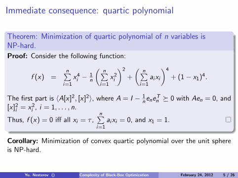
Immediate consequence: quartic polynomial

Theorem: Minimization of quartic polynomial of n variables isNP-hard.

Proof: Consider the following function:

f (x) =n∑

i=1x4i −

1n

(n∑

i=1x2i

)2

+

(n∑

i=1aixi

)4

+ (1− x1)4.

The first part is 〈A[x ]2, [x ]2〉, where A = I − 1nene

Tn � 0 with Aen = 0, and

[x ]2i = x2i , i = 1, . . . , n.

Thus, f (x) = 0 iff all xi = τ ,n∑

i=1aixi = 0, and x1 = 1.

Corollary: Minimization of convex quartic polynomial over the unit sphereis NP-hard.


Nonlinear Optimal Control: NP-hard

Problem: minu{ f (x(1)) : x ′ = g(x , u), 0 ≤ t ≤ 1, x(0) = x0 }.

Consider g(x , u) = 1nx · 〈x , u〉 − u.

Lemma. Let ‖x0‖2 = n. Then ‖x(t)‖2 = n, 0 ≤ t ≤ 1.

Proof. Consider g̃(x , u) =(

xxT

‖x‖2 − I)u and let x ′ = g̃(x , u). Then

〈x ′, x〉 = 〈(

xxT

‖x‖2 − I)u, x〉 = 0.

Thus, ‖x(t)‖2 = ‖x0‖2. Same is true for x(t) defined by g .Note: We have enough degrees of freedom to put x(1) at any position ofthe sphere.Hence, our problem is: min{f (y) : ‖y‖2 = n}.


Descent direction of nonsmooth nonconvex function

Consider φ(x) =(

1− 1γ

)max

1≤i≤n|xi | − min

1≤i≤n|xi |+ |〈a, x〉|,

where a ∈ Zn+ and γ

def=

n∑i=1

ai ≥ 1. Clearly, φ(0) = 0.

Lemma. It is NP-hard to decide if φ(x) < 0 for some x ∈ Rn.Proof: 1. Assume that σ ∈ Rn with σi = ±1 satisfies 〈a, σ〉 = 0. Thenφ(σ) = − 1

γ < 0.2. Assume φ(x) < 0 and max

1≤i≤n|xi | = 1. Denote δ = |〈a, x〉|.

Then |xi | > 1− 1γ + δ, i = 1, . . . , n.

Denoting σi = signxi , we have σixi > 1− 1γ + δ. Therefore,

|σi − xi | = 1− σixi < 1γ − δ, and we conclude that

|〈a, σ〉| ≤ |〈a, x〉|+ |〈a, σ − x〉| ≤ δ + γ max1≤i≤n

|σi − xi |

< (1− γ)δ + 1 ≤ 1.

Since a ∈ Zn , this is possible iff 〈a, σ〉 = 0.


Black-box optimization

Oracle: Special unit for computing function value and derivatives at testpoints. (0-1-2 order.)

Analytic complexity: Number of calls of oracle, which is necessary(sufficient) for solving any problem from the class.

(Lower/Upper complexity bounds.)

Solution: ε-approximation of the minimum.

Resisting oracle: creates the worst problem instance for a particularmethod.

Starts from “empty” problem.

Answers must be compatible with the description of the problem class.

The bad problem is created after the method stops.


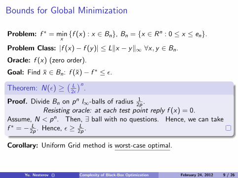
Bounds for Global Minimization

Problem: f ∗ = minx{f (x) : x ∈ Bn}, Bn = {x ∈ Rn : 0 ≤ x ≤ en}.

Problem Class: |f (x)− f (y)| ≤ L‖x − y‖∞ ∀x , y ∈ Bn.

Oracle: f (x) (zero order).

Goal: Find x̄ ∈ Bn: f (x̄)− f ∗ ≤ ε.

Theorem: N(ε) ≥(

L2ε

)n.

Proof. Divide Bn on pn l∞-balls of radius 12p .

Resisting oracle: at each test point reply f (x) = 0.Assume, N < pn. Then, ∃ ball with no questions. Hence, we can takef ∗ = − L

2p . Hence, ε ≥ L2p .

Corollary: Uniform Grid method is worst-case optimal.


Nonsmooth Convex Minimization (NCM)

Problem: f ∗ = minx{f (x) : x ∈ Q}, where

Q ⊆ Rn is a convex set: x , y ∈ Q ⇒ [x , y ] ∈ Q. It is simple.

f (x) is a sub-differentiable convex function:

f (y) ≥ f (x) + 〈f ′(x), y − x〉, x , y ∈ Q,

for certain subgradient f ′(x) ∈ Rn.

Oracle: f (x), f ′(x) (first order).

Solution: ε-approximation in function value.

Main inequality: 〈f ′(x), x − x∗〉 ≥ f (x)− f ∗ ≥ 0, ∀x ∈ Q.

NB: Anti-subgradient decreases the distance to the optimum.


NCM: Lower Complexity Bounds

.Let Q ≡ {‖x‖ ≤ 2R} and xk+1 ∈ x0 + Lin{f ′(x0), . . . , f ′(xk)}.Consider the function fm(x) = L max

1≤i≤mxi + µ

2‖x‖2 with µ = L

Rm1/2 .

From the problem: minτ

(Lτ + µm

2 τ2), we get

τ∗ = − Lµm = − R

m1/2 , f∗m = − L2

2µm = − LRm1/2 , ‖x∗‖2 = mτ2

∗ = R2.

NB: If x0 = 0, then after k iterations we can keep xi = 0 for i > k .

Lipschitz continuity: fk+1(xk)− f ∗k+1 ≥ −f ∗k+1 = LR(k+1)1/2 .

Strong convexity: fk+1(xk)− f ∗k+1 ≥ −f ∗k+1 = L2

2(k+1)·µ .

Both lower bounds are exact!


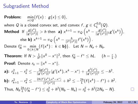
Subgradient Method

Problem: minx∈Q{f (x) : g(x) ≤ 0},

where Q is a closed convex set, and convex f , g ∈ C 0,0L (Q).

Method If g(xk )‖g ′(xk )‖ > h then a) xk+1 = πQ

(xk − g(xk )

‖g ′(xk )‖2 g′(xk)

),

else b) xk+1 = πQ

(xk − h

‖f ′(xk )‖ f′(xk)

).

Denote f ∗N = min0≤k≤N

{f (xk) : k ∈ b)}. Let N = Na + Nb.

Theorem: If N > 1h2 ‖x0 − x∗‖2, then f ∗N − f ∗ ≤ hL. (h = ε

L .)

Proof: Denote rk = ‖xk − x∗‖.

a): r2k+1 − r2

k ≤ −2g(xk )‖g ′(xk )‖2 〈g ′(xk), xk − x∗〉+ g2(xk )

‖g ′(xk )‖2 ≤ −h2.

b): r2k+1 − r2

k ≤ −2h〈f ′(xk ),xk−x∗〉‖f ′(xk )‖ + h2 ≤ −2h

L (f (xk)− f ∗) + h2.

Thus, Nb2hL (f ∗N − f ∗) ≤ r2

0 + h2(Nb − Na) = r20 + h2(2Nb − N).


Smooth Convex Minimization (SCM)

Lipschitz-continuous gradient: ‖f ′(x)− f ′(y)‖ ≤ L‖x − y‖.Geometric interpretation: for all x , y ∈ domF we have

0 ≤ f (y)− f (x)− 〈f ′(x), y − x〉

=1∫

0

〈f ′(x + τ(y − x)− f ′(x), y − x〉dt ≤ L2‖x − y‖2.

Sufficient condition: 0 � f ′′(x) � L · In, x ∈ dom f .

Equivalent definition:

f (y) ≥ f (x) + 〈f ′(x), y − x〉+ 12L‖f

′(x)− f ′(y)‖2.

Hint: Prove first that f (x)− f ∗ ≥ 12L‖f

′(x)‖2.


SCM: Lower complexity bounds

Consider the family of functions (k ≤ n):

fk(x) = 12

[x2

1 +k−1∑i=1

(xi − xi+1)2 + x2k

]− x1 ≡ 1

2〈Akx , x〉 − x1.

Let Rnk = {x ∈ Rn : xi = 0, i > k}. Then fk+p(x) = fk(x), x ∈ Rn

k .

Clearly, 0 ≤ 〈Akh, h〉 ≤ h21 +

k−1∑i=1

2(h2i + h2

i+1) + h2k ≤ 4‖h‖2,

Ak =

2 −1 0−1 2 −1

0 −1 20

. . . . . .

0−1 2 −1

0 −1 2

k lines

0n−k,k 0n−k,n−k

,


Hence, Akx = e1 has the solution x̄ki =

{k+1−ik+1 , 1 ≤ i ≤ k ,

0, i > k ..

Thus f ∗k = 12〈Ak x̄

k , x̄k〉 − 〈e1, x̄k〉 = −1

2〈e1, x̄k〉 = − k

2(k+1) , and

‖ x̄k ‖2=k∑

i=1

(k+1−ik+1

)2= 1

(k+1)2

k∑i=1

i2 = k(2k+1)6(k+1) .

Let x0 = 0 and p ≤ n is fixed.

Lemma. If xk ∈ Lkdef= Lin{f ′p(x0), . . . , f ′p(xk−1)}, then Lk ⊆ Rn

k .

Proof: x0 = 0 ∈ Rn0 , f′p(0) = −e1 ∈ Rn

1 ⇒ x1 ∈ Rn1 , f′p(x1) ∈ Rn

2 ,�

Corollary 1: fp(xk) = fk(xk) ≥ f ∗k .

Corollary 2: Take p = 2k + 1. Thenfp(xk )−f ∗pL‖x0−x̄p‖2 ≥

[− k

2(k+1) + 2k+12(2k+2)

]/[

(2k+1)(4k+3)3(k+1)

]= 3

4(2k+1)(4k+3) .

‖ xk − x̄p ‖2≥2k+1∑i=k+1

(x̄2k+1i )2 = (2k+3)(k+2)

24(k+1) ≥ 18‖x̄

p‖2.


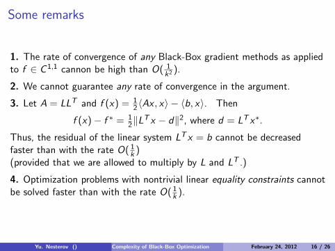
Some remarks

1. The rate of convergence of any Black-Box gradient methods as appliedto f ∈ C 1,1 cannon be high than O( 1

k2 ).

2. We cannot guarantee any rate of convergence in the argument.

3. Let A = LLT and f (x) = 12〈Ax , x〉 − 〈b, x〉. Then

f (x)− f ∗ = 12‖L

T x − d‖2, where d = LT x∗.

Thus, the residual of the linear system LT x = b cannot be decreasedfaster than with the rate O( 1

k )(provided that we are allowed to multiply by L and LT .)

4. Optimization problems with nontrivial linear equality constraints cannotbe solved faster than with the rate O( 1

k ).


Methods for Smooth Minimization with Simple Constraints

Consider the problem: minx{f (x) : x ∈ Q},

where convex f ∈ C 1,1L (Q), and Q is a simple closed convex set (allows

projections).

Gradient mapping: for M > 0 defineTM(x) = arg min

y∈Q[f (x) + 〈f ′(x), y − x〉+ M

2 ‖x − y‖2].

If M ≥ L, thenf (TM(x)) ≤ f (x) + 〈f ′(x),TM(x)− x〉+ M

2 ‖x − TM(x)‖2].

Reduced gradient: gM(x) = M · (x − TM(x)).

Since 〈f ′(x) + M(TM(x)− x), y − TM(x)〉 ≥ 0 for all y ∈ Q,

f (x)− f (TM(x)) ≥ M2 ‖x − TM(x)‖2 = 1

2M ‖gM(x)‖2, (→ 0)

f (y) ≥ f (x) + 〈f ′(x),TM(x)− x〉+ 〈f ′(x), y − TM(x)〉≥ f (TM(x))− 1

2M ‖gM(x)‖2 + 〈gM(x), y − TM(x)〉.


Primal Gradient Method (PGM)

Main scheme: x0 ∈ Q, xk+1 = TL(xk), k ≥ 0.

Primal interpretation: xk+1 = πQ(xk − 1

L f′(xk)

).

Rate of convergence. f (xk)− f (xk+1) ≥ 12L‖gL(xk)‖2.

f (TL(x))− f ∗ ≤ 12L‖gL(x)‖2 + 〈gL(x),TL(x)− x∗〉

≤ 12L(‖gL(x)‖+ LR)2 − L

2R2.

Hence, ‖gL(x)‖ ≥[2L(f (TL(x))− f ∗) + L2R2

]1/2 − LR

= 2L(f (TL(x))−f ∗)[2L(f (TL(x))−f ∗)+L2R2]1/2+LR

≥ cR · (f (TL(x))− f ∗).

Thus, f (xk)− f (xk+1) ≥ c2

LR2 (f (xk+1)− f ∗)2.

Similar situation: a′(t) = −a2(t)⇒ a(t) ≈ 1t .

Conclusion: PGM converges as O( 1k ). This is far from the lower

complexity bounds.


Dual Gradient Method (DGM)

Model: Let λki ≥ 0, i = 0, . . . , k, and Skdef=

k∑i=0

λki . Then

Sk f (y) ≥ Lλk (y)def=

k∑i=0

λki [f (x i ) + 〈f ′(x i ), y − x i 〉], y ∈ Q.

Our method: xk+1 = arg miny∈Q

{ψk(y)

def= Lλk (y) + M

2 ‖y − x0‖2}

.

Let us choose λki ≡ 1 and M = L. We prove by induction

(∗) : F ∗kdef=

k∑i=0

f (y i ) ≤ ψ∗kdef= min

y∈Qψk(y). (≤ (k + 1)f ∗ + L

2R2)

1. k = 0. Then y0 = TL(x0).2. Assume (∗) is true for some k ≥ 0. Then

ψ∗k+1 = miny∈Q

[ψk(y) + f (xk) + 〈f ′(xk), y − xk〉

]≥ min

y∈Q

[ψ∗k + L

2‖y − xk‖2 + f (xk) + 〈f ′(xk), y − xk〉].

We can take yk+1 = TL(xk). Thus, 1k+1

k∑i=0

f (y i ) ≤ f ∗ + LR2

2(k+1) .


Some remarks

1. Dual gradient method works with the model of the objective function.

2. The minimizing sequence {yk} is not necessary for the algorithmicscheme. We can generate it if necessary.

3. Both primal and dual method have the same rate of convergence O( 1k ).

It is not optimal.

May be we can combine them in order to get a better rate?


Comparing PGM and DGM

Primal Gradient method

Monotonically improves the current state using the local model of theobjective.

Interpretation: Practitioners, industry.

Dual Gradient Method

The main goal is to construct a model of the objective.

It is updated by a new experience collected around the predicted testpoints (xk).

Practical verification of the advices (yk) is not essential for theprocedure.

Interpretation: Science.

Hint: Combination of theory and practice should give better results


Estimating sequences

Def. A sequences {φk(x)}∞k=0 and {λk}∞k=0, λk ≥ 0 are called theestimating sequences if λk → 0 and ∀x ∈ Q, k ≥ 0,

(∗) : φk(x) ≤ (1− λk)f (x) + λkφ0(x).

Lemma: If (∗∗) : f (xk) ≤ φ∗k ≡ minx∈Q

φk(x), then

f (xk)− f ∗ ≤ λk [φ0(x∗)− f ∗]→ 0.

Proof. f (xk) ≤ φ∗k = minx∈Q

φk(x) ≤ minx∈Q

[(1− λk)f (x) + λkφ0(x)]

≤ (1− λk)f (x∗) + λkφ0(x∗). �

Rate of λk → 0 defines the rate of f (xk)→ f ∗.

Questions

How to construct the estimating sequences?

How we can ensure (**)?


Updating estimating sequences

Let φ0(x) = L2‖x − x0‖2, λ0 = 1, {yk}∞k=0 is a sequence in Q, and

{αk}∞k=0 : αk ∈ (0, 1),∞∑k=0

αk =∞. Then {φk(x)}∞k=0, {λk}∞k=0:

λk+1 = (1− αk)λk ,

φk+1(x) = (1− αk)φk(x) + αk [f (yk) + 〈f ′(yk), x − yk〉]are estimating sequences.Proof: φ0(x) ≤ (1− λ0)f (x) + λ0φ0(x) ≡ φ0(x).If (*) holds for some k ≥ 0, then

φk+1(x) ≤ (1− αk)φk(x) + αk f (x)= (1− (1− αk)λk)f (x) + (1− αk)(φk(x)− (1− λk)f (x))≤ (1− (1− αk)λk)f (x) + (1− αk)λkφ0(x)= (1− λk+1)f (x) + λk+1φ0(x). �


Updating the points

Denote φ∗k = minx∈Q

φk(x), vk = arg minx∈Q

φk(x). Suppose φ∗k ≥ f (xk).

φ∗k+1 = minx∈Q

{(1− αk)φk(x) + αk [f (yk) + 〈f ′(yk), x − yk〉]

}≥

minx∈Q

{(1− αk)[φ∗k + λkL

2 ‖x − vk‖2] + αk [f (yk) + 〈f ′(yk), y − yk〉]}

≥ minx∈Q{f (yk) + (1−αk )λkL

2 ‖x − vk‖2

+〈f ′(yk), αk(x − yk) + (1− αk)(xk − yk)〉}(yk

def= (1− αk)xk + αkv

k = xk + αk(vk − xk))

= minx∈Q{f (yk) + (1−αk )λkL

2 ‖x − vk‖2 + αk〈f ′(yk), x − vk〉}

= miny=xk+αk (x−xk )

x∈Q

{f (yk) + (1−αk )λkL2α2

k‖y − yk‖2 + 〈f ′(yk), y − yk〉}

(?)

≥ f (xk+1)

Answer: α2k = (1− αk)λk . xk+1 = TL(yk).


Optimal method

Choose v 0 = x0 ∈ Q, λ0 = 1, φ0(x) =L2‖x − x0‖2.

For k ≥ 0 iterate:

Compute αk : α2k = (1− αk)λk ≡ λk+1.

Define yk = (1− αk)xk + αkvk .

Compute xk+1 = TL(yk).

φk+1(x) = (1− αk)φk(x) + αk [f (yk) + 〈f ′(yk), x − yk〉].

Convergence: Denote ak = λ−1/2k . Then

ak+1 − ak =λ

1/2k −λ

1/2k+1

λ1/2k λ

1/2k+1

= λk−λk+1

λ1/2k λ

1/2k+1(λ

1/2k +λ

1/2k+1)≥ λk−λk+1

2λkλ1/2k+1

= αk

2λ1/2k+1

= 12 .

Thus, ak ≥ 1 + k2 . Hence, λk ≤ 4

(k+2)2 .


Interpretation

1. φk(x) accumulates all previously computed information about theobjective. This is a current model of our problem.2. vk = arg min

x∈Qφk(x) is a prediction of the optimal strategy.

3. φ∗k = φk(vk) is an estimate of the optimal value.

4. Acceleration condition: f (xk) ≤ φ∗k . We need a firm, which is atleast as good as the best theoretical prediction.5. Then we create a startup yk = (1−αk)xk +αkv

k , and allow it to workone year.

6. Theorem: Next year, its performance will be at least as good as thenew theoretical prediction. And we can continue!

Acceleration result: 10 years instead 100.

Who is in a right position to arrange 5? Government, politicalinstitutions.


Documents

Lecture 1: Intrinsic complexity of Black-Box Optimizationfrancqui/slides/Lect1_Complexity... · Standard Complexity Classes Let data be coded in matrix A, and n be dimension of the