Embed Size (px)
Citation preview
Importance Sampling for Reinforcement Learning
with Multiple Objectives
by
Christian Robert Shelton
B.S., Leland Stanford Junior University (1996)
S.M., Massachusetts Institute of Technology (1998)
Submitted to the Department of Electrical Engineering and Computer
Science in Partial Fulfillment of the Requirements for the Degree of
Doctor of Philosophy in Electrical Engineering and Computer Science
at the
MASSACHUSETTS INSTITUTE OF TECHNOLOGY
August 2001
c© Massachusetts Institute of Technology 2001. All rights reserved.
Author . . . . . . . . . . . . . . . . . . . . . . . . . . . . . . . . . . . . . . . . . . . . . . . . . . . . . . . . . . . . . .Department of Electrical Engineering and Computer Science
August 20, 2001
Certified by. . . . . . . . . . . . . . . . . . . . . . . . . . . . . . . . . . . . . . . . . . . . . . . . . . . . . . . . . .Tomaso Poggio
Professor of Brain and Cognitive Science
Thesis Supervisor
Accepted by . . . . . . . . . . . . . . . . . . . . . . . . . . . . . . . . . . . . . . . . . . . . . . . . . . . . . . . . .
Arthur C. SmithChairman, Departmental Committee on Graduate Students

2
Importance Sampling for Reinforcement Learning with
Multiple Objectives
by
Christian Robert Shelton
Submitted to the Department of Electrical Engineering and Computer Scienceon August 20, 2001, in partial fulfillment of the requirements for the Degree of
Doctor of Philosophy in Electrical Engineering and Computer Science
Abstract
This thesis considers three complications that arise from applying reinforcement learn-ing to a real-world application. In the process of using reinforcement learning tobuild an adaptive electronic market-maker, we find the sparsity of data, the partialobservability of the domain, and the multiple objectives of the agent to cause seriousproblems for existing reinforcement learning algorithms.
We employ importance sampling (likelihood ratios) to achieve good performancein partially observable Markov decision processes with few data. Our importancesampling estimator requires no knowledge about the environment and places fewrestrictions on the method of collecting data. It can be used efficiently with reac-tive controllers, finite-state controllers, or policies with function approximation. Wepresent theoretical analyses of the estimator and incorporate it into a reinforcementlearning algorithm.
Additionally, this method provides a complete return surface which can be used tobalance multiple objectives dynamically. We demonstrate the need for multiple goalsin a variety of applications and natural solutions based on our sampling method. Thethesis concludes with example results from employing our algorithm to the domainof automated electronic market-making.
Thesis Supervisor: Tomaso PoggioTitle: Professor of Brain and Cognitive Science
3

4

This thesis describes research done within the Department of Electrical Engineer-ing and Computer Science and the Department of Brain & Cognitive Sciences withinthe Center for Biological & Computational Learning and the Artificial IntelligenceLaboratory at the Massachusetts Institute of Technology.
This research was sponsored by grants from Office of Naval Research (DARPA)under contract No. N00014-00-1-0907, National Science Foundation (ITR) under con-tract No. IIS-0085836, National Science Foundation (KDI) under contract No. DMS-9872936, and National Science Foundation under contract No. IIS-9800032.
Additional support was provided by: Central Research Institute of Electric PowerIndustry, Center for e-Business (MIT), Eastman Kodak Company, DaimlerChryslerAG, Compaq, Honda R&D Co. Ltd., Komatsu Ltd., Merrill-Lynch, NEC Fund, Nip-pon Telegraph & Telephone, and Siemens Corporate Research, Inc., Toyota MotorCorporation, and The Whitaker Foundation.
I know this thesis would have been more difficult and of lesser quality were it not forthe patience and trust of my advisor,the flexibility and approachability of my committee,the academic and social support of the AI Lab graduate students,and the faith and love of my parents.
Thank you.
5

6

Contents
1 Introduction 13
1.1 Task Description . . . . . . . . . . . . . . . . . . . . . . . . . . . . . 14
1.1.1 Agent-Environment Cycle . . . . . . . . . . . . . . . . . . . . 17
1.1.2 Example Domains . . . . . . . . . . . . . . . . . . . . . . . . . 18
1.1.3 Environment Knowledge . . . . . . . . . . . . . . . . . . . . . 18
1.2 Environment Models . . . . . . . . . . . . . . . . . . . . . . . . . . . 19
1.2.1 POMDP Model . . . . . . . . . . . . . . . . . . . . . . . . . . 19
1.2.2 MDP Model . . . . . . . . . . . . . . . . . . . . . . . . . . . . 21
1.2.3 Previous Work . . . . . . . . . . . . . . . . . . . . . . . . . . 22
1.3 Contribution . . . . . . . . . . . . . . . . . . . . . . . . . . . . . . . . 25
2 Importance Sampling for Reinforcement Learning 29
2.1 Notation . . . . . . . . . . . . . . . . . . . . . . . . . . . . . . . . . . 30
2.2 Overview of Importance Sampling . . . . . . . . . . . . . . . . . . . . 30
2.3 Previous Work . . . . . . . . . . . . . . . . . . . . . . . . . . . . . . 31
2.4 Importance Sampling Estimator . . . . . . . . . . . . . . . . . . . . . 32
2.4.1 Sampling Ratios . . . . . . . . . . . . . . . . . . . . . . . . . . 33
2.4.2 Importance Sampling as Function Approximation . . . . . . . 33
2.4.3 Normalized Estimates . . . . . . . . . . . . . . . . . . . . . . 36
2.5 Estimator Properties . . . . . . . . . . . . . . . . . . . . . . . . . . . 37
2.6 Policy Improvement Algorithm . . . . . . . . . . . . . . . . . . . . . 41
2.7 Results . . . . . . . . . . . . . . . . . . . . . . . . . . . . . . . . . . . 44
7
3 Extensions of Importance Sampling 45
3.1 Memory . . . . . . . . . . . . . . . . . . . . . . . . . . . . . . . . . . 45
3.1.1 Finite State Machine Model . . . . . . . . . . . . . . . . . . . 46
3.1.2 Memory Ratios . . . . . . . . . . . . . . . . . . . . . . . . . . 46
3.1.3 Hidden Markov Models . . . . . . . . . . . . . . . . . . . . . . 48
3.1.4 Results . . . . . . . . . . . . . . . . . . . . . . . . . . . . . . . 49
3.2 Function Approximation . . . . . . . . . . . . . . . . . . . . . . . . . 53
3.2.1 Policy Weights . . . . . . . . . . . . . . . . . . . . . . . . . . 53
3.2.2 Results . . . . . . . . . . . . . . . . . . . . . . . . . . . . . . . 55
3.3 Controlled Search . . . . . . . . . . . . . . . . . . . . . . . . . . . . . 56
4 Balancing Multiple Goals 61
4.1 Rewards as Goals . . . . . . . . . . . . . . . . . . . . . . . . . . . . . 62
4.1.1 Related Work . . . . . . . . . . . . . . . . . . . . . . . . . . . 63
4.1.2 Notation . . . . . . . . . . . . . . . . . . . . . . . . . . . . . . 64
4.2 Policy Equilibria . . . . . . . . . . . . . . . . . . . . . . . . . . . . . 64
4.2.1 Policy Climbing . . . . . . . . . . . . . . . . . . . . . . . . . . 65
4.2.2 Algorithm . . . . . . . . . . . . . . . . . . . . . . . . . . . . . 68
4.2.3 Results . . . . . . . . . . . . . . . . . . . . . . . . . . . . . . . 68
4.3 Bounded Maximization . . . . . . . . . . . . . . . . . . . . . . . . . . 71
4.3.1 Algorithm . . . . . . . . . . . . . . . . . . . . . . . . . . . . . 71
4.3.2 Results . . . . . . . . . . . . . . . . . . . . . . . . . . . . . . . 72
5 Electronic Market-Making 75
5.1 Market-Making . . . . . . . . . . . . . . . . . . . . . . . . . . . . . . 75
5.1.1 Automating Market-Making . . . . . . . . . . . . . . . . . . . 76
5.1.2 Previous Work . . . . . . . . . . . . . . . . . . . . . . . . . . 77
5.2 Simple Model . . . . . . . . . . . . . . . . . . . . . . . . . . . . . . . 79
5.2.1 Model Description . . . . . . . . . . . . . . . . . . . . . . . . 80
5.2.2 Theoretical Analysis . . . . . . . . . . . . . . . . . . . . . . . 82
5.2.3 Results . . . . . . . . . . . . . . . . . . . . . . . . . . . . . . . 84
8

5.3 Spread Model . . . . . . . . . . . . . . . . . . . . . . . . . . . . . . . 89
5.3.1 Model Description . . . . . . . . . . . . . . . . . . . . . . . . 90
5.3.2 Results . . . . . . . . . . . . . . . . . . . . . . . . . . . . . . . 90
5.4 Discussion . . . . . . . . . . . . . . . . . . . . . . . . . . . . . . . . . 93
6 Conclusions 95
6.1 Algorithm Components . . . . . . . . . . . . . . . . . . . . . . . . . . 96
6.1.1 Estimator Performance . . . . . . . . . . . . . . . . . . . . . . 96
6.1.2 Greedy Search . . . . . . . . . . . . . . . . . . . . . . . . . . . 97
6.1.3 Multiple Objectives . . . . . . . . . . . . . . . . . . . . . . . . 98
6.2 Market-Making . . . . . . . . . . . . . . . . . . . . . . . . . . . . . . 99
A Bias and Variance Derivations 101
A.1 Unnormalized Estimator . . . . . . . . . . . . . . . . . . . . . . . . . 102
A.2 Unnormalized Differences . . . . . . . . . . . . . . . . . . . . . . . . . 104
A.3 Normalized Differences . . . . . . . . . . . . . . . . . . . . . . . . . . 105
9

10
List of Figures
1-1 Block diagram of the reinforcement learning setting . . . . . . . . . . 15
1-2 RL algorithm plot . . . . . . . . . . . . . . . . . . . . . . . . . . . . . 26
2-1 Nearest-neighbor partitioning . . . . . . . . . . . . . . . . . . . . . . 34
2-2 Empirical estimates of means and standard deviations . . . . . . . . . 40
2-3 Left-right world . . . . . . . . . . . . . . . . . . . . . . . . . . . . . . 42
2-4 Comparison of normalized and unnormalized importance sampling . . 43
3-1 Memory model graph . . . . . . . . . . . . . . . . . . . . . . . . . . . 46
3-2 Load-unload world . . . . . . . . . . . . . . . . . . . . . . . . . . . . 50
3-3 Blind load-unload world . . . . . . . . . . . . . . . . . . . . . . . . . 51
3-4 Comparison of REINFORCE to normalized importance sampling . . 51
3-5 Comparison of external and internal memory . . . . . . . . . . . . . . 52
3-6 Fully-observable left-right world returns . . . . . . . . . . . . . . . . . 56
3-7 Importance sampling for fully-observable left-right world . . . . . . . 57
3-8 Hypothetical one-dimensional example . . . . . . . . . . . . . . . . . 58
4-1 Joint maximization search algorithm . . . . . . . . . . . . . . . . . . 67
4-2 Cooperate world . . . . . . . . . . . . . . . . . . . . . . . . . . . . . 69
4-3 Cooperate comparison . . . . . . . . . . . . . . . . . . . . . . . . . . 70
4-4 Robot collision world . . . . . . . . . . . . . . . . . . . . . . . . . . . 73
4-5 Collision verses time . . . . . . . . . . . . . . . . . . . . . . . . . . . 74
5-1 Theoretical basic model profits . . . . . . . . . . . . . . . . . . . . . . 83
5-2 Basic model noise . . . . . . . . . . . . . . . . . . . . . . . . . . . . . 84
11
5-3 Sample market-making runs . . . . . . . . . . . . . . . . . . . . . . . 85
5-4 Sample market-making episodes . . . . . . . . . . . . . . . . . . . . . 85
5-5 Basic model results . . . . . . . . . . . . . . . . . . . . . . . . . . . . 86
5-6 Noise dependence . . . . . . . . . . . . . . . . . . . . . . . . . . . . . 87
5-7 Imbalance/spread interaction . . . . . . . . . . . . . . . . . . . . . . 91
5-8 Spread verses profit . . . . . . . . . . . . . . . . . . . . . . . . . . . . 91
12

Chapter 1
Introduction
“A little learning is a dangerous thing.”
Essay on Criticism. part ii. line 15.
Alexander Pope
Designing the control algorithm for the robot can be difficult for many robotic
tasks. The physical world is highly variable: the same exact situation seldom arises
twice, measurements of the world are noisy, much of the important information for a
decision is hidden, and the exact dynamics of the environment are usually unknown.
When the robot is created, we may not be able to anticipate all possible situations and
tasks. In many applications, writing software to explicitly control the robot correctly
is difficult if not impossible.
Similar situations arise in other areas of control. Virtual robots, or software agents,
have similar difficulties navigating and solving problems in electronic domains. Agents
that search the world wide web for prices or news stories, programs that trade securi-
ties electronically, and software for planning travel itineraries are all becoming more
popular. They don’t operate in the physical world, but their virtual environments
have many of the same characteristics. The agents have actions they can take, such
as requesting information from online services or presenting data to the user. They
have observations they make, such as the web page provided by a server or the user’s
current choice. And they have goals, such as finding the best price for a book or
13
finding the quickest way to travel from New York to Los Angeles.
This thesis considers learning as a tool to aid in the design of robust algorithms
for environments which may not be completely known ahead of time. We begin in
this chapter by describing reinforcement learning, some of its background, and the
relationship of this work to other algorithms and methods. Chapter 2 develops the
main algorithm and theoretical contributions of the thesis. Chapters 3 and 4 extend
this algorithm to deal with more complex controllers, noisy domains, and multiple
simultaneous goals. Chapter 5 uses these techniques to design an adaptive electronic
market-maker. We conclude in chapter 6 by discussing the contribution of this work
and possible future directions.
1.1 Task Description
A learning algorithm has the potential to be more robust than an explicit control algo-
rithm. Most programmed control policies are designed by beginning with assumptions
about the environment’s dynamics and the goal behavior. If the assumptions are in-
correct, this can lead to critically suboptimal behavior. Learning algorithms begin
with few assumptions about the environment dynamics and therefore less often fail
due to incorrect assumptions. However, as with all adaptive methods, the trade-off is
that the algorithm may perform poorly initially while learning. The relaxed assump-
tions come at the cost of a more general model of the environment. In order to be
effective, the algorithm must use experience to fill in the details of the environment
that the designer left unspecified.
In practice, it is not unsurprising that hybrid systems that have adaptation for
some parts and engineered preset knowledge for other parts are the most successful.
Yet, for this work, we will try to make only the most necessary assumptions so as to
push the learning aspects of agent control as far as possible.
There are a number of separate fields of learning within artificial intelligence. Su-
pervised learning is the most common. In a supervised learning scenario, the agent
is presented with a number of example situations and the corresponding correct re-
14
π
environment
reward
agent
observation action
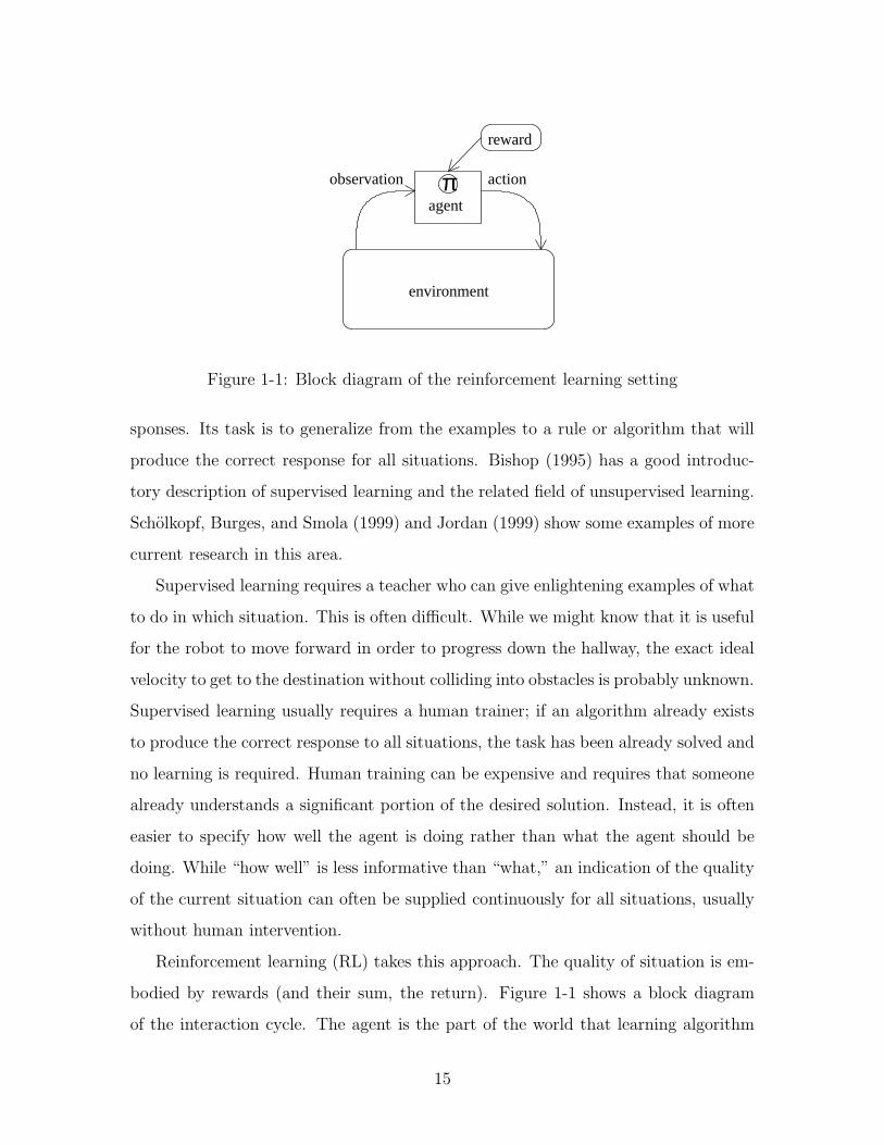
Figure 1-1: Block diagram of the reinforcement learning setting
sponses. Its task is to generalize from the examples to a rule or algorithm that will
produce the correct response for all situations. Bishop (1995) has a good introduc-
tory description of supervised learning and the related field of unsupervised learning.
Scholkopf, Burges, and Smola (1999) and Jordan (1999) show some examples of more
current research in this area.
Supervised learning requires a teacher who can give enlightening examples of what
to do in which situation. This is often difficult. While we might know that it is useful
for the robot to move forward in order to progress down the hallway, the exact ideal
velocity to get to the destination without colliding into obstacles is probably unknown.
Supervised learning usually requires a human trainer; if an algorithm already exists
to produce the correct response to all situations, the task has been already solved and
no learning is required. Human training can be expensive and requires that someone
already understands a significant portion of the desired solution. Instead, it is often
easier to specify how well the agent is doing rather than what the agent should be
doing. While “how well” is less informative than “what,” an indication of the quality
of the current situation can often be supplied continuously for all situations, usually
without human intervention.
Reinforcement learning (RL) takes this approach. The quality of situation is em-
bodied by rewards (and their sum, the return). Figure 1-1 shows a block diagram
of the interaction cycle. The agent is the part of the world that learning algorithm
15

controls. In our examples above, the agent would be the robot or the internet appli-
cation. The environment encompasses all of the rest of the world. In general, we limit
this to be only the parts of the world that have a measurable effect on the agent. The
symbol π is used to stand for the controlling policy of the agent. The reinforcement
learning algorithm’s job is to find a policy that maximizes the return.
The reward is not part of either the agent or the environment but is a function
of one or both of them. The task of the agent is to maximize the return, the total
reward over all time. It might be in the agent’s best interest to act such as to decrease
the immediate reward if that leads to greater future rewards. The agent needs to
consider the long-term consequences of its actions in order to achieve its objective.
The reward defines the agent’s objective and is a fixed part of the problem’s definition.
Whether it is defined by the system’s designers or is a signal from the environment
is left unspecified. For the purposes of this thesis, it is assumed to be fixed prior to
invoking learning.
All parts of this model are unknown to the learning algorithm. The learning algo-
rithm knows the interface to the world (the set of possible actions and observations),
but no more. The dynamics of the environment, the meaning of the observations,
the effects of actions, and the reward function are all unknown to the agent. As the
agent interacts with the environment, it experiences observations and rewards as it
tries actions. From this experience, the algorithm’s job is to select a control policy
for the agent that will, in expectation, maximize the total reward.
Narrowing the definition can be difficult without omitting some type of reinforce-
ment learning. Kaelbling, Littman, and Moore (1996) do a good job of describing
the many aspects to reinforcement learning and the range of the different approaches.
The definition of return, the type of controller, and the knowledge about the task do-
main can vary. Yet, two properties are universal to almost all reinforcement learning
research: time passes in discrete increments and the return is the sum of rewards, one
per time step.
16
1.1.1 Agent-Environment Cycle
The discrete nature implies that the environment and the agent take turns (or are at
least modeled that way). The system is a closed loop and thus the output generated
by the agent affects the output generated by the environment and, symmetrically,
the environment affects the agent. These changes are sequential and occur in time
steps. Usually the environment is considered to be fixed to begin the cycle and the
description takes an agent-centric point-of-view. The environment’s output is called
an observation (because it is what the agent senses about the environment) and the
agent’s output is called an action (because it is what the agent uses to affect the
environment). The agent senses the current observation from the environment; the
agent executes its controller policy to select an action; and the environment changes
in response to the action (thus affecting the next observation). This completes one
time step after which the cycle repeats.
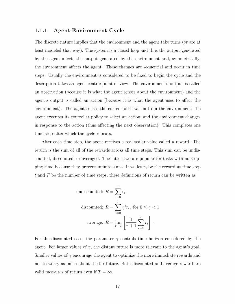
After each time step, the agent receives a real scalar value called a reward. The
return is the sum of all of the rewards across all time steps. This sum can be undis-
counted, discounted, or averaged. The latter two are popular for tasks with no stop-
ping time because they prevent infinite sums. If we let rt be the reward at time step
t and T be the number of time steps, these definitions of return can be written as
undiscounted: R =
T∑
t=0
rt
discounted: R =T∑
t=0
γtrt, for 0 ≤ γ < 1
average: R = limτ→T
[
1
τ + 1
τ∑
t=0
rt
]
.
For the discounted case, the parameter γ controls time horizon considered by the
agent. For larger values of γ, the distant future is more relevant to the agent’s goal.
Smaller values of γ encourage the agent to optimize the more immediate rewards and
not to worry as much about the far future. Both discounted and average reward are
valid measures of return even if T =∞.
17
1.1.2 Example Domains
We can now instantiate our robot and internet search scenarios from before, as re-
inforcement learning problems. In the case of electronic trading, the agent would
be the trading program and the environment would consist of the other traders and
the trading system. Actions might include placing bids on the market and querying
news agencies for financial stories. Observations would include the current value of
the traded securities, headlines from news sources, the current status of placed bids,
and text from requested articles. The most obvious reward would be the current
estimated value of the portfolio. The agent’s task would be to request information
and trade securities to maximize the value of its portfolio.
For robot navigation, the set of observations might be the current values of the
sensors on the robot (e.g., sonars, laser range finder, bump sensors). The actions
allowed might be settings of the motor voltages for the robot. At each time step, the
robot would receive a positive reward if it successfully navigated to the mail room and
a negative reward if it collided with a wall. The learning task would be to find a control
policy that drives the robot to the mail room as quickly as possible without colliding
with walls. We could also take a higher level view and provide the RL algorithm with
more broad statistics of the sensor readings and change the set of actions to be target
velocities or positions for fixed control subroutines (like PID controllers). With this
more abstract view of the problem, the provided fixed procedures for sensor fusion
and motor control become part of the environment from the RL problem formulation
standpoint. This is a common method to provide domain knowledge to reinforcement
learning algorithms in the form of known useful subroutines.
1.1.3 Environment Knowledge
Generally, it is assumed that the RL algorithm has no a priori knowledge about
the environment except to know the valid choice of actions and the set of possible
observations. This is what defines RL as a learning task. By trying actions or policies,
the algorithm gains information about the environment which it can use to improve
18
its policy. A fundamental struggle in reinforcement learning is achieving a balance
between the knowledge gained by trying new things and the benefit of using the
knowledge already gained to select a good policy. This is known as the exploration-
exploitation trade-off and it pits immediate knowledge benefits against immediate
return benefits. Although maximizing the return is the overall goal of the algorithm,
gaining knowledge now might lead to greater returns in the future.
1.2 Environment Models
To aid in addressing RL in a mathematically principled fashion, the environment
is usually assumed to be describable by a particular mathematical model. We first
outline two of the basic models and then describe the types of RL algorithms that
have been studied in conjunction with these models.
1.2.1 POMDP Model
The most general commonly-used model is a partially observable Markov decision
process (POMDP). A POMDP consists of seven elements: S,A,X , ps, px, p0, r. They
are:
• S is the set of all possible environment states. It is often called the state space.
• A is the set of all agent actions. It is often called the action space.
• X is the set of all observations. It is often called the observation space.
• ps is a probability distribution over S conditioned on a value from S×A. It the
probability of the world being in a particular state conditioned on the previous
world state and the action the agent took and is often written as ps(st|at−1, st−1).
• px is a probability distribution over X conditioned on a value from S. It is the
probability of an observation conditioned on the state of the world and is often
written as px(xt|st).
19

• p0 is a probability distribution over S. It is the probability that the world begins
in a particular state and is often written p0(s0).
• r is a function from S to the real numbers. It is the reward the agent receives
after the world transitions to a state and is often written as r(s).
The generative POMDP model is run as follows. To begin, s0 (the state at time
step 0) is picked at random from the distribution p0. From that point on, for each
time step t (beginning with t = 0), the following four steps occur:
1. The agent receives reward r(st).
2. Observation xt is drawn from the distribution px(xt|st).
3. The agent observes xt and makes calculations according to its policy. This
results in it producing at, the action for this time step.
4. The new world state st+1 is drawn from the distribution ps(st+1|at, st).
After these four steps, the time index increase (i.e., t← t+1) and the process repeats.
There are variations on this basic POMDP definition. The reward can depend
not only on the current state, but also on the last action taken. This new model
can be reduced to a POMDP of the form above with an increase in the size of S.
The POMDP definition above can also be simplified either by making the start state
deterministic, by making the observation a deterministic function of the state, or
by making the transition function deterministic. Any of these three (although not
more than one) simplifications can be placed on the POMDP model above without
changing the class of environments modeled. Again, however, any of these changes
might affect the size of S. Finally, the action space can be modified to depend on the
observation space. This can have an effect on the problem difficulty but complicates
the mathematical description unnecessarily for our purposes.
The POMDP model is Markovian in the state sequence. In particular, if one knows
the current state of the system and all of the internals of the agent, no additional
information about past states, observations, or actions will change one’s ability to
20
predict the future of the system. Unfortunately, this information is not available to
the agent. The agent, while knowing its own internal system, does not observe the
state of the environment. Furthermore, in the general case, it does not know any of
the probability distributions associated with the environment (ps, px, p0), the state
space of the environment (S), or the reward function (r). It is generally assumed,
however, that the agent knows the space of possible observations and actions (X and
A respectively). The observations may contain anywhere from complete information
about the state of the system to no information about the state of the system. It
depends on the nature of the unknown observation probability distribution, px.
1.2.2 MDP Model
The POMDP model is difficult to work with because of the potential lack of infor-
mation available to the agent. The MDP, Markov decision process, model can be
thought of as a specific form of the POMDP model for which the observation space
is the same as the state space (i.e., X = S) and the observation is always exactly
equal to the state (i.e. px(x|s) is 1 if x = s and 0 otherwise). Thus the model is fully
observable: the agent observes the true state of the environment. The only other
difference from the POMDP model is that the reward function is now stochastic to
make the learning problem slightly more difficult. Formally, it is best to remove the
observation from consideration entirely. The MDP consists then of five elements:
S,A,R, ps, p0, pr. They are:
• S is the set of all possible environment states (state space).
• A is the set of all agent actions (action space).
• R is the set of possible rewards. R ⊂ <.
• ps is a probability distribution over S conditioned on a value from S×A. It the
probability of the world being in a particular state conditioned on the previous
world state and the action the agent took and is often written as ps(st|at−1, st−1).
21
• p0 is a probability distribution over S. It is the probability that the world begins
in a particular state and is often written p0(s0).
• pr is a probability distribution over R conditioned on a value from S. It is
the probability of a reward conditioned on the current world state and is often
written as pr(rt|st).
The generative MDP model is run very similarly to the POMDP model. The
beginning state s0 is picked at random from p0 as before. Three steps occur for each
time step:
1. The reward rt is drawn from the distribution pr(rt|st).
2. The agent observes st and makes calculations according to its policy. This
results in it producing at, the action for this time step.
3. The new world state st+1 is drawn from the distribution ps(st+1|at, st).
After these three steps, the time index increases (i.e., t ← t + 1) and the process
repeats.
MDP models are often augmented by allowing the reward probability distribution
to depend also on the action taken by the agent. This does change the model slightly,
but not significantly for our considerations. Just as in the POMDP case, the MDP
definition is sometimes augmented to allow the action set to depend on the state of the
environment. This also slightly, but not significantly, changes the model. Although
the agent observes the true state value at each time step, ps, po, and pr are still
unknown. However, estimating them or functions of them is much easier than it
would be for POMDPs because samples from the distributions are directly observed.
1.2.3 Previous Work
Value functions are the single most prevalent reinforcement learning concept. They
do not play a role in this thesis, but are useful in understanding other algorithms. It
is beyond the scope of this thesis to fully describe value functions, but we will outline
their definition and use briefly.
22
Two types of value functions exist. V-values are associated with states and Q-
values are associated with state-action pairs. Informally, V π(s) is the return expected
if the environment is in state s and the agent is executing policy π. Qπ(s, a) is the
expected return if the environment is in state s, the agent executes action a and then
on subsequent time steps the agent executes policy π.
Because in an MDP the agent can observe the true state of the system, it can
estimate the quality (or value) of its current situation as represented by the value
functions. The current state, as mentioned before, provides as much information as
possible to predict the future and thereby the rewards that the agent is likely to
experience later.
The most popular value function methods are temporal difference (TD) algo-
rithms, the best known variants of which are Q-learning and SARSA. Sutton and
Barto (1998) provide a nice unified description of these algorithms. In temporal
difference algorithms, the value functions are updated by considering temporally ad-
jacent state values and adjusting the corresponding value function estimates to be
consistent. As an example, if the problem definition uses undiscounted reward, then
consistent value functions will have the property that
V π(st) = E[rt + V π(st+1)]
for any state st. This expresses that the value of being in a state at time t should
be equal to the expected reward plus the expected value of the next state. V π(st)
should represent all future rewards. They can be broken down into the immediate
next reward and all rewards that will occur after the environment reaches its next
state (V π(st+1)). By keeping track of all value function values and modifying them
carefully, a consistent value function can be estimated from experience the agent
gathers by interacting with the environment. One possible method is for the agent to
adjust the value of V π(st) towards the sum of the next reward and the value function
at the next state. This uses the interactions with the environment to sample the
expectation in the above equation.
23
Such methods have been very well studied and for environments which adhere to
the MDP model, they work consistently and well. In particular for MDPs, we do not
need to keep a separate value function for each policy. A number of methods exist for
estimating the value function for the optimal policy (even if the policy is unknown)
while learning. Once the value function has converged, it is simple to extract the
optimal policy from it. Bertsekas and Tsitsiklis (1996) give a nice mathematical
treatment of the convergence conditions for temporal difference methods in MDPs.
Yet, TD algorithms do not solve all problems. In many situations, the space of
states and actions is large. If value function estimates must be maintained for every
state-action pair, the number of estimated quantities is too big for efficient calculation.
The amount of experience needed grows with the number of quantities to estimate.
Furthermore, we might expect that many such estimates would have similar values
which might be able to be grouped together or otherwise approximated to speed up
learning. In general, we would hope be to be able to represent the value function with
a parameterized estimator instead of a large table of values, one for each state-action
pair. Unfortunately, while some approximators forms do yield convergence guarantees
(Boyan and Moore 1995), the class of allowable approximators is restricted.
For environments that are not fully observable, the situation is worse. The general
POMDP problem is quite difficult. Even if the model is known (and therefore no
learning needs to take place, the model must only be evaluated), finding the best
policy is PSPACE-hard (Littman 1996) for the finite time episodic tasks of this thesis.
Therefore, it is more reasonable to search for the optimal policy within a fixed class
of policies or to settle for a locally optimal policy of some form. Unfortunately,
temporal difference methods cannot yet do either. TD, SARSA, and Q-learning can
all be shown to fail to converge to the correct best policy for some simple POMDP
environments. While Q-learning can be shown to diverge in such situations, TD
and SARSA have been shown to converge to a region. Unfortunately, the region
of convergence is so large as to be useless (Gordon 2001). Thus, no performance
guarantees can be made for any of these algorithms if run on POMDP problems.
However, value functions can be otherwise extended to POMDPs. Actor-critic
24
methods have been used to extend value function methods to partially observable
domains. Jaakkola, Singh, and Jordan (1995) and Williams and Singh (1999) present
one such method and Konda and Tsitsiklis (2000) and Sutton, McAllester, Singh,
and Mansour (2000) describe another. They use value function estimation on a fixed
policy (this type of estimation is stable) to estimate the value for that policy and then
improve their policy according to the gradient of the expected return of the policy
as estimated by the value function. After each policy change, the old value function
estimates must be thrown away and the new ones recomputed from scratch in order
to maintain convergence guarantees.
Other more direct methods for POMDPs also exist. REINFORCE (Williams
1992) is the most classic and enduring RL algorithm for POMDPs. In this method,
each policy trial is used to adjust the policy slightly and is then discarded. No value
functions are required. It is similar to an actor-critic algorithm where the value
function estimation is performed using only a single trial of the policy. In fact the
hope of actor-critic methods such as that of Sutton, McAllester, Singh, and Mansour
(2000) is that the use of a value function would reduce the variance of the gradient
estimate and lead to faster convergence in comparison to REINFORCE. However,
initial theoretical results (McAllester 2000) seem to indicate that there is no extra
gain with such a variance reduction. In fact, the update rule may be the same in
formula and differ only in method of calculation.
VAPS (Baird and Moore 1999) is a different method for using value methods with
POMDP environments. It combines the criteria from REINFORCE and SARSA to
create a single algorithm. It is relatively new and its success is as of yet unevaluated.
1.3 Contribution
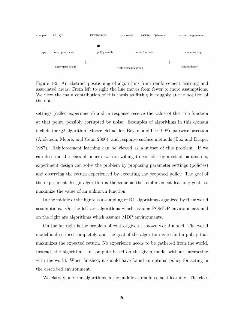
Figure 1-2 shows one possible ranking of algorithms from fewest to most assumptions
about the world. On the far left is the problem of function maximization from limited
stochastic samples. In this problem, the goal of the algorithm is to find the parameters
that maximize a particular unknown function. The algorithm can propose parameter
25
value functions model solvingpolicy search
experiment design reinforcement learning control theory
REINFORCE actor-criticPB1, Q2
type:
example: SARSA Q-learning
noisy optimization
dynamic programming
Figure 1-2: An abstract positioning of algorithms from reinforcement learning andassociated areas. From left to right the line moves from fewer to more assumptions.We view the main contribution of this thesis as fitting in roughly at the position ofthe dot.
settings (called experiments) and in response receive the value of the true function
at that point, possibly corrupted by noise. Examples of algorithms in this domain
include the Q2 algorithm (Moore, Schneider, Boyan, and Lee 1998), pairwise bisection
(Anderson, Moore, and Cohn 2000), and response surface methods (Box and Draper
1987). Reinforcement learning can be viewed as a subset of this problem. If we
can describe the class of policies we are willing to consider by a set of parameters,
experiment design can solve the problem by proposing parameter settings (policies)
and observing the return experienced by executing the proposed policy. The goal of
the experiment design algorithm is the same as the reinforcement learning goal: to
maximize the value of an unknown function.
In the middle of the figure is a sampling of RL algorithms organized by their world
assumptions. On the left are algorithms which assume POMDP environments and
on the right are algorithms which assume MDP environments.
On the far right is the problem of control given a known world model. The world
model is described completely and the goal of the algorithm is to find a policy that
maximizes the expected return. No experience needs to be gathered from the world.
Instead, the algorithm can compute based on the given model without interacting
with the world. When finished, it should have found an optimal policy for acting in
the described environment.
We classify only the algorithms in the middle as reinforcement learning. The class
26
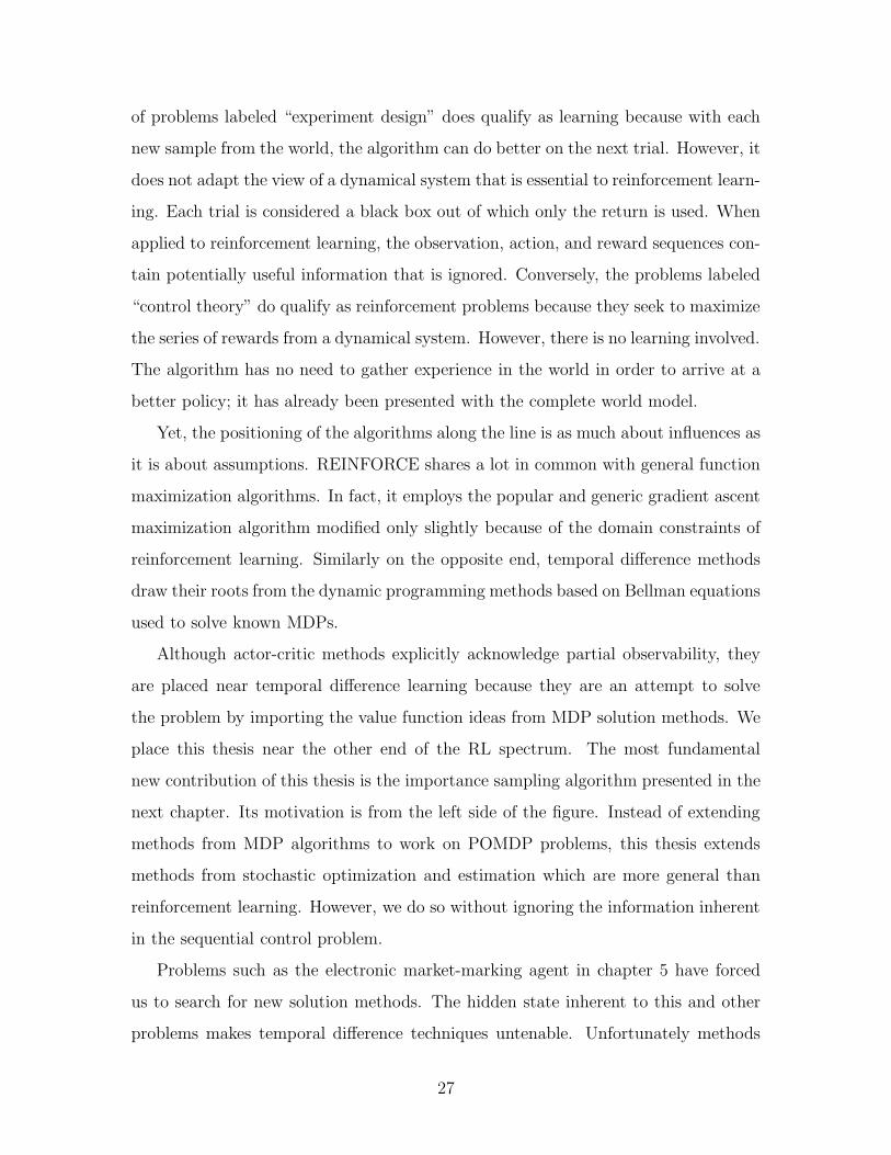
of problems labeled “experiment design” does qualify as learning because with each
new sample from the world, the algorithm can do better on the next trial. However, it
does not adapt the view of a dynamical system that is essential to reinforcement learn-
ing. Each trial is considered a black box out of which only the return is used. When
applied to reinforcement learning, the observation, action, and reward sequences con-
tain potentially useful information that is ignored. Conversely, the problems labeled
“control theory” do qualify as reinforcement problems because they seek to maximize
the series of rewards from a dynamical system. However, there is no learning involved.
The algorithm has no need to gather experience in the world in order to arrive at a
better policy; it has already been presented with the complete world model.
Yet, the positioning of the algorithms along the line is as much about influences as
it is about assumptions. REINFORCE shares a lot in common with general function
maximization algorithms. In fact, it employs the popular and generic gradient ascent
maximization algorithm modified only slightly because of the domain constraints of
reinforcement learning. Similarly on the opposite end, temporal difference methods
draw their roots from the dynamic programming methods based on Bellman equations
used to solve known MDPs.
Although actor-critic methods explicitly acknowledge partial observability, they
are placed near temporal difference learning because they are an attempt to solve
the problem by importing the value function ideas from MDP solution methods. We
place this thesis near the other end of the RL spectrum. The most fundamental
new contribution of this thesis is the importance sampling algorithm presented in the
next chapter. Its motivation is from the left side of the figure. Instead of extending
methods from MDP algorithms to work on POMDP problems, this thesis extends
methods from stochastic optimization and estimation which are more general than
reinforcement learning. However, we do so without ignoring the information inherent
in the sequential control problem.
Problems such as the electronic market-marking agent in chapter 5 have forced
us to search for new solution methods. The hidden state inherent to this and other
problems makes temporal difference techniques untenable. Unfortunately methods
27

aimed at POMDPs such as REINFORCE and actor-critic architectures forget all
previous data each time the policy is modified. For RL to be a viable solution method,
it must learn quickly and efficiently. We, therefore, need a method that makes use
of all of the data to make maximally informed decisions. Finally, we found that
most problems from real applications do not have a single obvious reward function.
Designing multiple reward functions separately, each to describe a different objective
of the agent, is simpler and leads to more natural designs. The techniques of this
thesis are designed to address these three considerations: partial observability, scarce
data, and multiple objectives.
We make what we feel are a minimal number of assumptions about reinforcement
learning and develop an algorithm to solve this general problem. Such an approach
is not without flaws. Most problems are not as difficult as the most general reinforce-
ment learning problem can be. By making few assumptions, the algorithm is inclined
to treat all problems as equally and maximally difficult. Because this thesis presents a
novel solution method, we have concentrated on theoretical and experimental results
for the algorithm’s most basic forms. However, we feel confident that, despite its
current generality, useful biases and heuristics can be added to allow better perfor-
mance on practical applications. We are not convinced that all of the useful biases are
towards full observability and value function approaches. By starting from the other
end of the spectrum we hope to develop a framework that more easily allows for the
incorporation of other types of heuristics and information. We do not dismiss the use-
fulness of values functions and temporal difference algorithms; we present this work
as an alternative approach. Hopefully the connection between the two approaches
will become clearer in the future.
28
Chapter 2
Importance Sampling for
Reinforcement Learning
“Solon gave the following advice: ‘Consider your honour, as a
gentleman, of more weight than an oath. Never tell a lie. Pay
attention to matters of importance.’ ”
Solon. xii.
Diogenes Laertius
In this chapter, we jump right in and develop an algorithm for reinforcement
learning based on importance sampling and greedy search.
There are a number of different ways to organize the experience of the agent. For
this thesis, we use the episodic formulation. The agent’s experience is grouped into
episodes or trials. At the beginning of each trial, the environment is reset (the state
is drawn from p0). The agent interacts with the environment until the end of the
trial when the environment is reset again and the cycle continues. The agent is aware
of the trial resets. We are using fixed-length episodes: a trial lasts for a set number
of time steps. The current time step index may or may not be available as part of
the observations (it is not available for any the problems in this thesis). We use the
undiscounted return definition. Because the number of time steps is fixed, there are
no real differences among the various return definitions.
29
2.1 Notation
Throughout the thesis, we will use the following consistent notation to refer to the
experience data gathered by the agent. s represents the hidden state of the environ-
ment, x the observation, a the action, and r the reward. Subscripts denote the time
step within a trial and superscripts denote the trial number.
Let π(x, a) be a policy (the probability of picking action a upon observing x). For
this chapter, we will consider only reactive policies (policies that depend only on the
current observation and have no memory). Memory is added in the next chapter.
h represents a trial history1 (of T time steps). h is a tuple of four sequences:
states (s1 through sT ), observations (x1 through xT ), actions (a1 through aT ), and
rewards (r1 through rT ). The state sequence is not available to the algorithm and is
for theoretical consideration only. Any calculations performed by the algorithm must
depend only on the observation, action, and reward sequences. Lastly, we let R be
the return (the sum of r1 through rT ).
We assume the agent employs only one policy during each trial. Between trials,
the agent may change policies. π1 through πn are the n policies tried (n increases as
the agent experiences more trials). h1 through hn are the associated n histories with
R1 through Rn being the returns of those histories. Thus during trial i, the agent
executed policy πi resulting in the history hi. Ri is used as a shorthand notation for
R(hi), the return of trial i.
2.2 Overview of Importance Sampling
Importance sampling is typically presented as a method for reducing the variance of
the estimate of an expectation by carefully choosing a sampling distribution (Rubin-
stein 1981). For example, the most direct method for evaluating∫
f(x)p(x) dx is to
sample i.i.d. xi ∼ p(x) and use 1n
∑
i f(xi) as the estimate. However, by choosing
1It might be better to refer to this as a trajectory. We will not limit h to represent only sequencesthat have been observed; it can also stand for sequences that might be observed. However, thesymbol t is over-used already. Therefore, we have chosen to use h to represent state-observation-action-reward sequences.
30
a different distribution q(x) which has higher density in the places where |f(x)| is
larger, we can get a new estimate which is still unbiased and has lower variance. In
particular, we can draw xi ∼ q(x) and use 1n
∑
i f(xi)p(xi)q(xi)
as the new estimate. This
can be viewed as estimating the expectation of f(x) p(x)q(x)
with respect to q(x) which is
like approximating∫
f(x)p(x)q(x)
q(x) dx with samples drawn from q(x). If q(x) is chosen
properly, our new estimate has lower variance. It is always unbiased provided that
the support of p(x) and q(x) are the same. Because in this thesis we only consider
stochastic policies that have a non-zero probability of taking any action at any time,
our sampling and target distributions will always have the same support.
Instead of choosing q(x) to reduce variance, we will be forced to use q(x) because
of how our data was collected. Unlike the traditional setting where an estimator is
chosen and then a distribution is derived which will achieve minimal variance, we
have a distribution chosen and we are trying to find an estimator with low variance.
2.3 Previous Work
Kearns, Mansour, and Ng (2000) present a method for estimating the return for every
policy simultaneously using data gathered while executing a fixed policy. By contrast,
we consider the case where the policies used for gathering data are unrestricted. Either
we did not have control over the method for data collection, or we would like to allow
the learning algorithm the freedom to pick any policy for any trial and still be able
to use the data. Ng and Jordan (2000) give a method for estimating returns from
samples gathered under a variety of policies. However, their algorithm assumes the
environment is a simulation over which the learning algorithm has some control, such
as the ability to fix the random number sequence used to generate trials. Such an
assumption is impractical for non-simulated environments.
Importance sampling has been studied before in conjunction with reinforcement
learning. In particular, Precup, Sutton, and Singh (2000) and Precup, Sutton, and
Dasgupta (2001) use importance sampling to estimate Q-values for MDPs with func-
tion approximation for the case where all data have been collected using a single
31
policy. Meuleau, Peshkin, and Kim (2001) use importance sampling for POMDPs,
but to modify the REINFORCE algorithm (Williams 1992) and thereby discard trials
older than the most recent one. Peshkin and Mukherjee (2001) consider estimators
very similar to the ones developed here and prove theoretical PAC bounds for them.
This chapter differs from previous work in that it allows multiple sampling policies,
uses normalized estimators for POMDP problems, derives exact bias and variance for-
mulas for normalized and unnormalized estimators, and extends importance sampling
from reactive policies to finite-state controllers.
In this chapter we develop two estimators (unnormalized and normalized). Sec-
tion 2.5 shows that while the normalized estimator is biased, its variance is much
lower than the unnormalized (unbiased) estimator resulting in a better estimator for
comparisons. Section 2.7 demonstrates some results on a simulated environment.
2.4 Importance Sampling Estimator
Policy evaluation is the task of estimating the expected return of a fixed policy.
Many reinforcement learning algorithms use such an evaluation method as a key
part to maximizing the expected return, although there are algorithms which do not
explicitly compute expected returns.
Usually an RL algorithm will fix a policy to be evaluated (a target policy). It will
then perform either on-policy or off-policy evaluation. In the former, the algorithm
executes the target policy (possibly repeatedly) and uses the experience to evaluate
the expected return. In the latter, the algorithm executes a different policy and uses
the experience to evaluate the expected return of the target policy.
We will extend the generality slightly further. Instead of picking the target policy
ahead of time, we will allow the agent to collect experience with any desired series of
execution policies. We develop an estimator that can take this data and estimate the
expected return for any target policy. This will prove useful for efficient use of data.
32
2.4.1 Sampling Ratios
Every policy induces a probability distribution over histories. The probabilities asso-
ciated with the policy combined with the probabilities of the environment produce a
complete distribution over histories. The returns are a deterministic function of the
history. Therefore, we desire to calculate E[R(h)|π] where the expectation is taken
with respect to the history probability induced by the policy π.
A key observation is that we can calculate one factor in the probability of a history
given a policy. In particular, that probability has the form
p(h|π) = p(s0)
T∏
t=0
p(xt|st)π(xt, at)p(st+1|st, at)
=
[
p(s0)
T∏
t=0
p(xt|st)p(st+1|st, at)
][
T∏
t=0
π(xt, at)
]
4= W (h)A(h, π) .
A(h, π), the effect of the agent, is computable whereas W (h), the effect of the world,
is not because it depends on knowledge of the hidden state sequence. However, W (h)
does not depend on π. This implies that the ratios necessary for importance sampling
are exactly the ratios that are computable without knowing the state sequence. In
particular, if a history h was drawn according to the distribution induced by π and
we would like an unbiased estimate of the return of π′, then we can use R(h)p(h|π′)p(h|π)
and although neither the numerator nor the denominator of the importance sampling
ratio can be computed, the W (h) terms from each cancel, leaving the ratio of A(h, π ′)
to A(h, π) which can be calculated. A different statement of the same fact has been
shown before by Meuleau, Peshkin, and Kim (2001). This fact will be exploited in
each of the estimators of this thesis.
2.4.2 Importance Sampling as Function Approximation
Because each πi is potentially different, each hi is drawn according to a different
distribution and so while the data are drawn independently, they are not identically
33
1 2
3
45
6
7
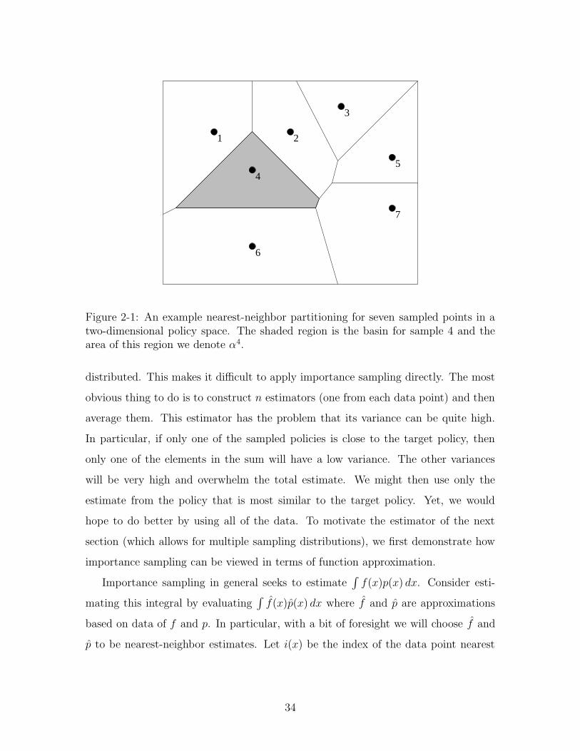
Figure 2-1: An example nearest-neighbor partitioning for seven sampled points in atwo-dimensional policy space. The shaded region is the basin for sample 4 and thearea of this region we denote α4.
distributed. This makes it difficult to apply importance sampling directly. The most
obvious thing to do is to construct n estimators (one from each data point) and then
average them. This estimator has the problem that its variance can be quite high.
In particular, if only one of the sampled policies is close to the target policy, then
only one of the elements in the sum will have a low variance. The other variances
will be very high and overwhelm the total estimate. We might then use only the
estimate from the policy that is most similar to the target policy. Yet, we would
hope to do better by using all of the data. To motivate the estimator of the next
section (which allows for multiple sampling distributions), we first demonstrate how
importance sampling can be viewed in terms of function approximation.
Importance sampling in general seeks to estimate∫
f(x)p(x) dx. Consider esti-
mating this integral by evaluating∫
f(x)p(x) dx where f and p are approximations
based on data of f and p. In particular, with a bit of foresight we will choose f and
p to be nearest-neighbor estimates. Let i(x) be the index of the data point nearest
34
to x. Then the nearest-neighbor approximations can be written as,
f(x) = f(xi(x))
p(x) = p(xi(x)) .
We now must define the size of the “basin” near sample xi. In particular we let αi
be the size of the region of the sampling space closest to xi. In the case where the
sampling space is discrete, this is the number of points which are closer to sampled
point xi than any other sampled point. For continuous sampling spaces, αi is the
volume of space which is closest to xi (see figure 2-1 for a geometric diagram). With
this definition,∫
f(x)p(x) dx =∑
i
αif(xi)p(xi) .
Both f and p are constant within a basin. We calculate the integral by summing over
each basin and multiplying by its volume.
αi cannot be computed and thus we need to approximate it as well. Let q(x)
be the distribution from which the data were sampled (we are still considering case
of a single sampling distribution). On average, we expect the density of points to
be inversely proportional to the volume nearest each point. For instance, if we have
sampled uniformly from a unit volume and the average density of points is d, then
the average volume nearest any given point is 1d. Extending this principle, we take
the estimate of αi to be inversely proportional to the sampling density at xi. That
is, αi = k 1q(xi)
. This yields the standard importance sampling estimator
∫
f(x)p(x) dx ≈1
n
∑
i
f(xi)p(xi)
q(xi).
More importantly, this derivation gives insight into how to merge samples from
different distributions, q1(x) through qn(x). Not until the estimation of αi did we
require knowledge about the sampling density. We can use the same approximations
for f and p. When estimating αi we need only an estimate of the density of points
35
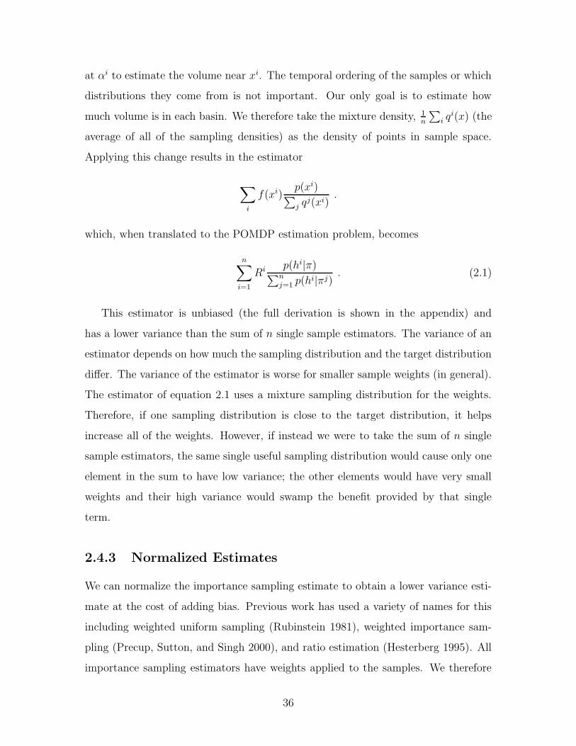
at αi to estimate the volume near xi. The temporal ordering of the samples or which
distributions they come from is not important. Our only goal is to estimate how
much volume is in each basin. We therefore take the mixture density, 1n
∑
i qi(x) (the
average of all of the sampling densities) as the density of points in sample space.
Applying this change results in the estimator
∑
i
f(xi)p(xi)
∑
j qj(xi).
which, when translated to the POMDP estimation problem, becomes
n∑
i=1
Ri p(hi|π)∑n
j=1 p(hi|πj). (2.1)
This estimator is unbiased (the full derivation is shown in the appendix) and
has a lower variance than the sum of n single sample estimators. The variance of an
estimator depends on how much the sampling distribution and the target distribution
differ. The variance of the estimator is worse for smaller sample weights (in general).
The estimator of equation 2.1 uses a mixture sampling distribution for the weights.
Therefore, if one sampling distribution is close to the target distribution, it helps
increase all of the weights. However, if instead we were to take the sum of n single
sample estimators, the same single useful sampling distribution would cause only one
element in the sum to have low variance; the other elements would have very small
weights and their high variance would swamp the benefit provided by that single
term.
2.4.3 Normalized Estimates
We can normalize the importance sampling estimate to obtain a lower variance esti-
mate at the cost of adding bias. Previous work has used a variety of names for this
including weighted uniform sampling (Rubinstein 1981), weighted importance sam-
pling (Precup, Sutton, and Singh 2000), and ratio estimation (Hesterberg 1995). All
importance sampling estimators have weights applied to the samples. We therefore
36
prefer the term normalized importance sampling to indicate that the weights sum to
one. Such an estimator has the form
∑
i f(xi)p(xi)q(xi)
∑
ip(xi)q(xi)
.
This normalized form can be viewed in three different ways. First, it can be seen just
as a trick to reduce variance. Second, it has been viewed as a Bayesian estimate of the
expectation (Geweke 1989; Kloek and van Dijk 1978). Unfortunately, the Bayesian
view does not work for our application because we do not know the true probabilities
densities. Hesterberg (1995) connects the ratio and Bayesian views, but neither can
be applied here.
Finally we can view the normalization as an adjustment to the function approx-
imator p. The problem with the previous estimator can be seen by noting that
the function approximator p(h) does not integrate (or sum) to 1. Instead of us-
ing p = p(xi(x)), we make sure p integrates (or sums) to 1: p = p(xi(x))/Z where
Z =∑
i αip(xi). When recast in terms of our POMDP problem the normalized
estimator is∑n
i=1 Ri p(hi|π)∑n
j=1p(hi|πj)
∑n
i=1p(hi|π)
∑nj=1
p(hi|πj)
. (2.2)
2.5 Estimator Properties
It is well known that importance sampling estimates (both normalized and unnormal-
ized) are consistent (Hesterberg 1995; Geweke 1989; Kloek and van Dijk 1978). This
means that as the number of sample grows without bound, the estimator converges
in the mean-squares sense to the true estimate. Additionally, normalized estimators
have smaller asymptotic variance if the sampling distribution does not exactly match
the distribution to estimate (Hesterberg 1995). However, our purpose behind using
importance sampling was to cope with few data. Therefore, we are more interested
in the case of finite sample sizes.
The estimator of equation 2.1 is unbiased. That is, for a set of chosen policies,
37

π1, π2, . . . , πn, the expectation of the estimate evaluated at π is the true expected
return for executing policy π. The expectation is over the probability of the histories
given the chosen policies. Similarly, the estimator of section 2.4.3 (equation 2.2) is
biased. In specific, it is biased towards the expected returns of π1, π2, . . . , πn.
The goal of constructing these estimators is to use them to choose a good policy.
This involves comparing the estimates for different values of π. Therefore instead of
considering a single point we will consider the difference of the estimator evaluated at
two different points, πA and πB. In other words, we will use the estimator to calculate
an estimate of the difference in expected returns between two policies. The difference
estimate uses the same data for both estimates at πA and πB.
We denote the difference in returns for the unnormalized estimator as DU and the
difference for the normalized estimator as DN . First, a few useful definitions (allowing
the shorthand RX = E[R|πX ] where X can stand for A or B):
p(h) =1
n
∑
i
p(h|πi)
p(h, g) =1
n
∑
i
p(h|πi)p(g|πi)
bA,B =
∫∫
[R(h)− R(g)]p(h|πA)p(g|πB)
p(h)p(g)p(h, g) dh dg
s2X,Y =
∫
R2(h)p(h|πX)p(h|πY )
p(h)dh
s2X,Y =
∫
(R(h)− RX)(R(h)−RY )p(h|πX)p(h|πY )
p(h)dh
η2X,Y =
∫∫
R(h)R(g)p(h|πX)p(g|πY )
p(h)p(g)p(h, g) dh dg
η2X,Y =
∫∫
(R(h)−RX)(R(g)− RY )
p(h|πX)p(g|πY )
p(h)p(g)p(h, g) dh dg
(2.3)
Note that all of these quantities are invariant to the number of samples provided that
the relative frequencies of the sampling policies remains fixed. p and p are measures
of the average sampling distribution. The other quantities are difficult to describe
intuitively. However, each of them has a form similar to an expectation integral.
38
s2X,Y and η2
X,Y are measures of second moments and s2X,Y and η2
X,Y are measures
of (approximately) centralized second moments.bA,B
nis the bias of the normalized
estimate of the return difference.
The means and variances are2
E[DU ] = RA − RB
E[DN ] = RA − RB −1
nbA,B
var[DU ] =1
n(s2
A,A − 2s2A,B + s2
B,B)
−1
n(η2
A,A − 2η2A,B + η2
B,B)
var[DN ] =1
n(s2
A,A − 2s2A,B + s2
B,B)
−1
n(η2
A,A − 2η2A,B + η2
B,B)
− 31
n(RA − RB)bA,B + O(
1
n2) .
(2.4)
The bias of the normalized return difference estimator and the variances of both
return difference estimators decrease as 1n. It is useful to note that if all of the
πi’s are the same, then p(h, g) = p(h)p(g) and thus bA,B = RA − RB. In this case
E[DN ] = n−1n
(RA − RB). If the estimator is only used for comparisons, this value is
just as good as the true return difference (of course, for small n, the same variance
would cause greater relative fluctuations).
In general we expect bA,B to be of the same sign as RA − RB. We would also
expect s2X,Y to be less than s2
X,Y and similarly η2X,Y to be less than η2
X,Y . s2X,Y and
η2X,Y depend on the difference of the returns from the expected return under πX
and πY . s2X,Y and η2
X,Y depend on the difference of the returns from zero. Without
any other knowledge of the underlying POMDP, we expect that the return from an
arbitrary history be closer to RA or RB than to the arbitrarily chosen value 0. If bA,B
is the same sign as the true difference in returns and the overlined values are less
2For the normalized difference estimator, the expectations shown are for the numerator of thedifference written as a single fraction. The denominator is a positive quantity and can be scaledto be approximately 1. Because the difference is only used for comparisons, this scaling makes nodifference in its performance. See the appendix for more details.
39
unnormalized normalized
mea
n
20 40 60 80 100
0
20
40
60
80
100
20 40 60 80 1000
5
10
15
20
25
30
35
std.dev
.
20 40 60 80 1000
1000
2000
3000
4000
5000
6000
7000
20 40 60 80 1000
2
4
6
8
10
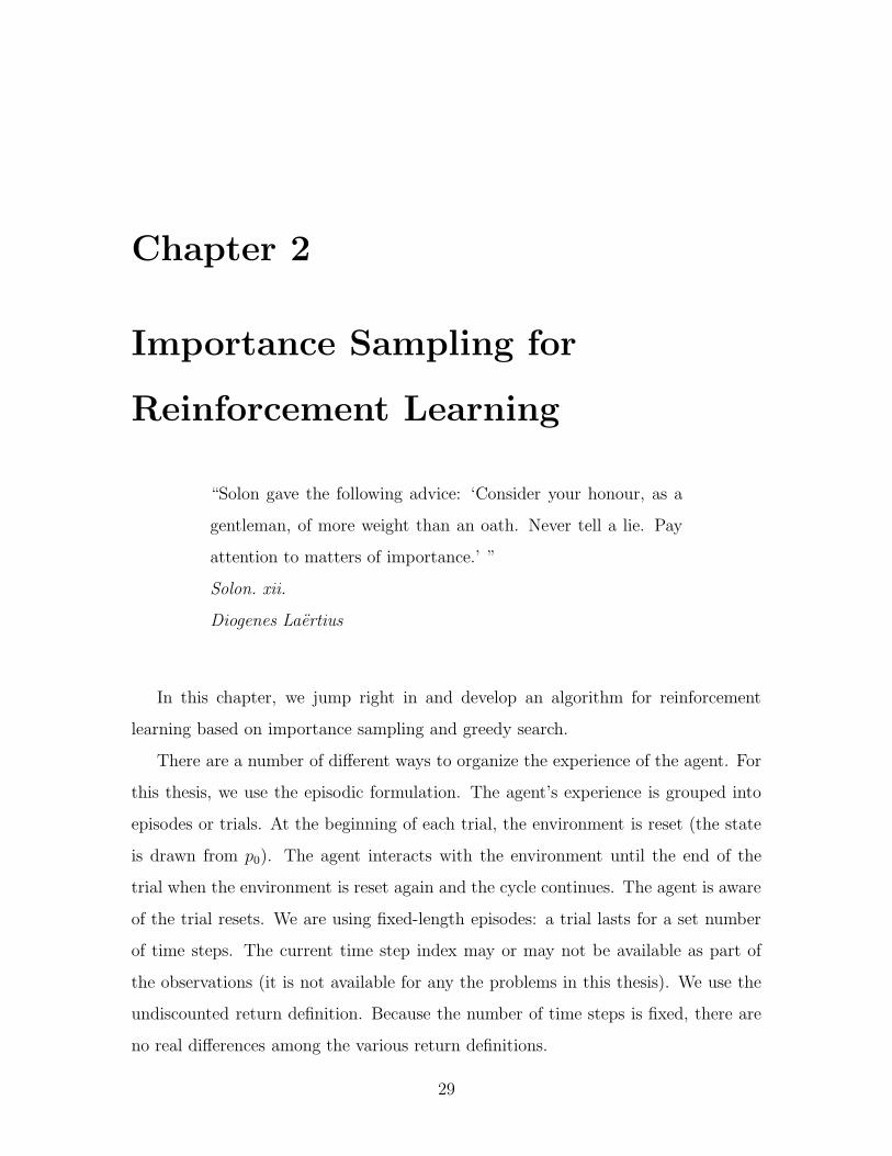
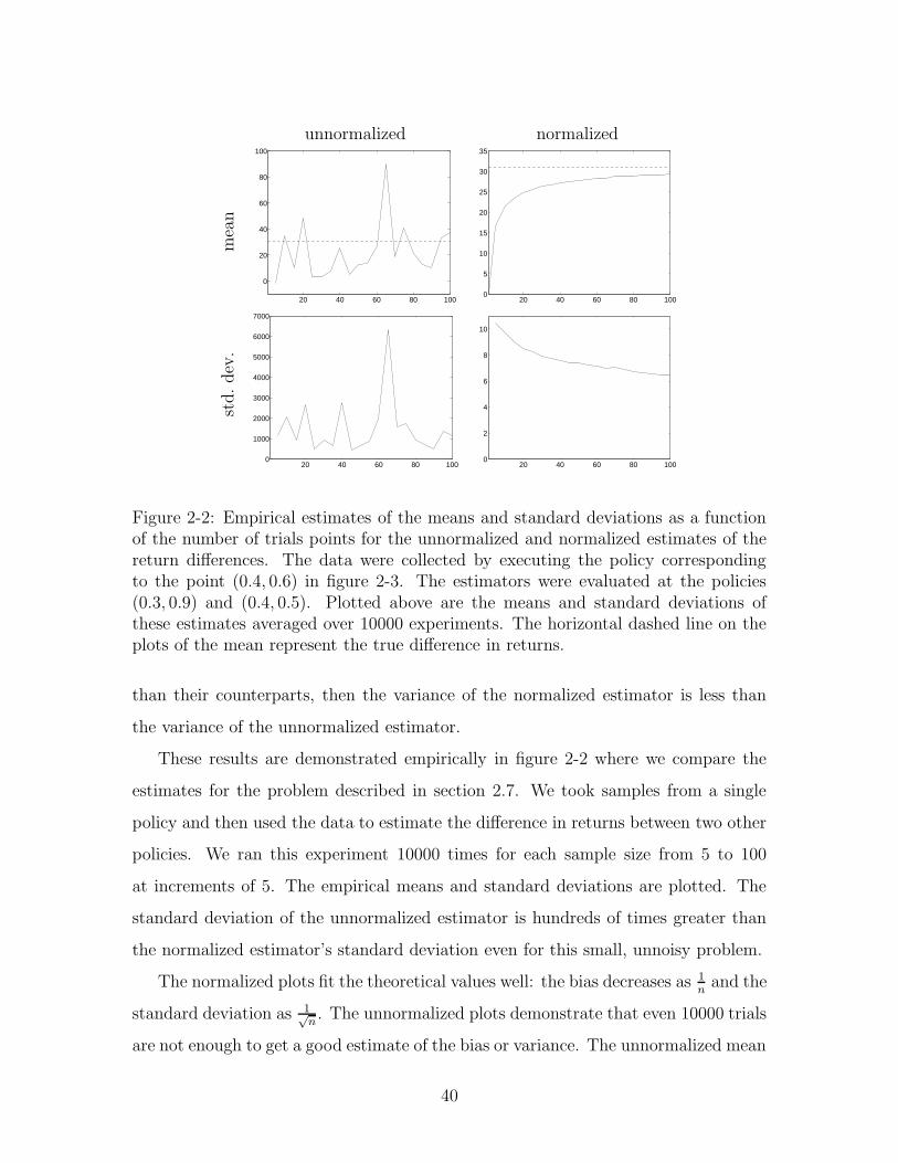
Figure 2-2: Empirical estimates of the means and standard deviations as a functionof the number of trials points for the unnormalized and normalized estimates of thereturn differences. The data were collected by executing the policy correspondingto the point (0.4, 0.6) in figure 2-3. The estimators were evaluated at the policies(0.3, 0.9) and (0.4, 0.5). Plotted above are the means and standard deviations ofthese estimates averaged over 10000 experiments. The horizontal dashed line on theplots of the mean represent the true difference in returns.
than their counterparts, then the variance of the normalized estimator is less than
the variance of the unnormalized estimator.
These results are demonstrated empirically in figure 2-2 where we compare the
estimates for the problem described in section 2.7. We took samples from a single
policy and then used the data to estimate the difference in returns between two other
policies. We ran this experiment 10000 times for each sample size from 5 to 100
at increments of 5. The empirical means and standard deviations are plotted. The
standard deviation of the unnormalized estimator is hundreds of times greater than
the normalized estimator’s standard deviation even for this small, unnoisy problem.
The normalized plots fit the theoretical values well: the bias decreases as 1n
and the
standard deviation as 1√n. The unnormalized plots demonstrate that even 10000 trials
are not enough to get a good estimate of the bias or variance. The unnormalized mean
40
should be constant at the true return difference (no bias) and the standard deviation
should decay as 1√n. However, because the unnormalized estimator is much more
asymmetric (it relies on a few very heavily weighted unlikely events to offset the more
common events), the graph does not correspond well to the theoretical values. This
is indicative of the general problem with the high variance unnormalized estimates.
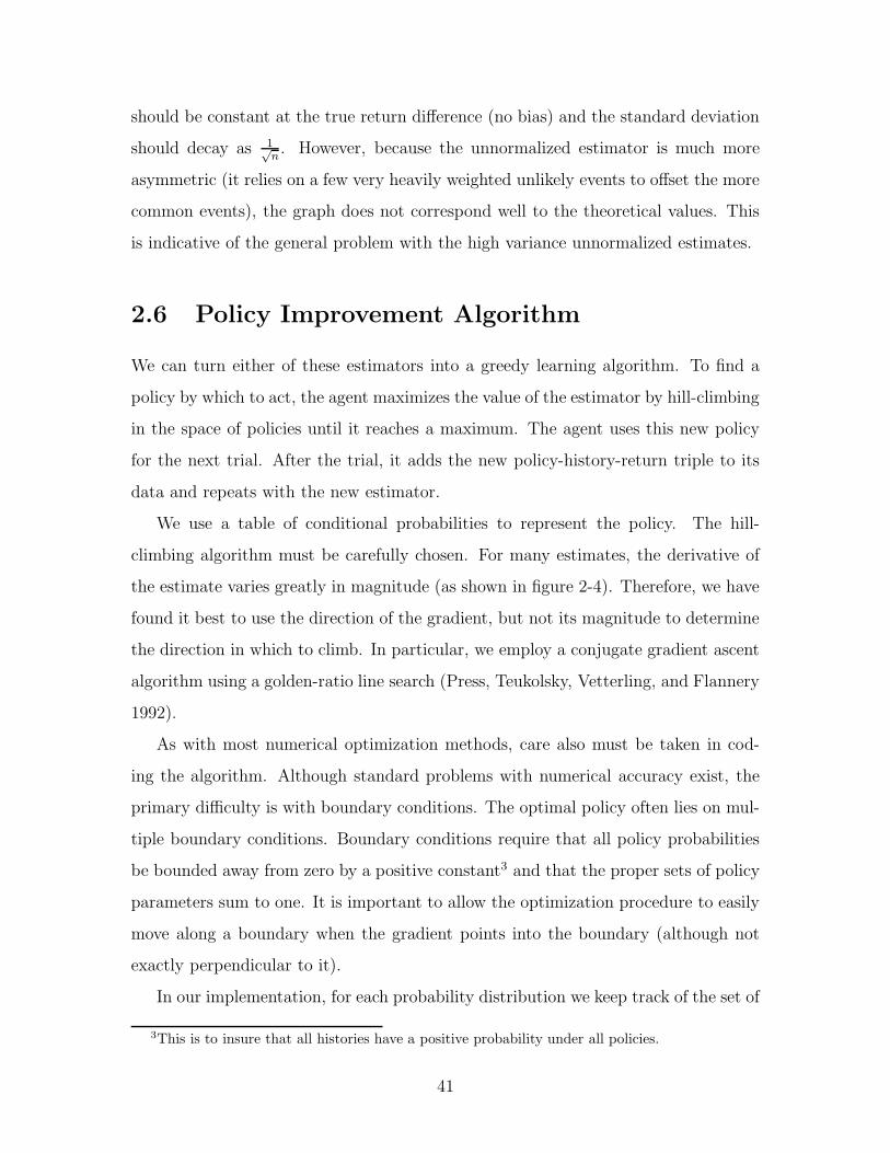
2.6 Policy Improvement Algorithm
We can turn either of these estimators into a greedy learning algorithm. To find a
policy by which to act, the agent maximizes the value of the estimator by hill-climbing
in the space of policies until it reaches a maximum. The agent uses this new policy
for the next trial. After the trial, it adds the new policy-history-return triple to its
data and repeats with the new estimator.
We use a table of conditional probabilities to represent the policy. The hill-
climbing algorithm must be carefully chosen. For many estimates, the derivative of
the estimate varies greatly in magnitude (as shown in figure 2-4). Therefore, we have
found it best to use the direction of the gradient, but not its magnitude to determine
the direction in which to climb. In particular, we employ a conjugate gradient ascent
algorithm using a golden-ratio line search (Press, Teukolsky, Vetterling, and Flannery
1992).
As with most numerical optimization methods, care also must be taken in cod-
ing the algorithm. Although standard problems with numerical accuracy exist, the
primary difficulty is with boundary conditions. The optimal policy often lies on mul-
tiple boundary conditions. Boundary conditions require that all policy probabilities
be bounded away from zero by a positive constant3 and that the proper sets of policy
parameters sum to one. It is important to allow the optimization procedure to easily
move along a boundary when the gradient points into the boundary (although not
exactly perpendicular to it).
In our implementation, for each probability distribution we keep track of the set of
3This is to insure that all histories have a positive probability under all policies.
41

j j j j j j jY Y Y Y Y Y Y
: 9
0
0.5
1
0
0.5
10
20
40
60
80
p(left | left)p(left | right)
expe
cted
ret
urn
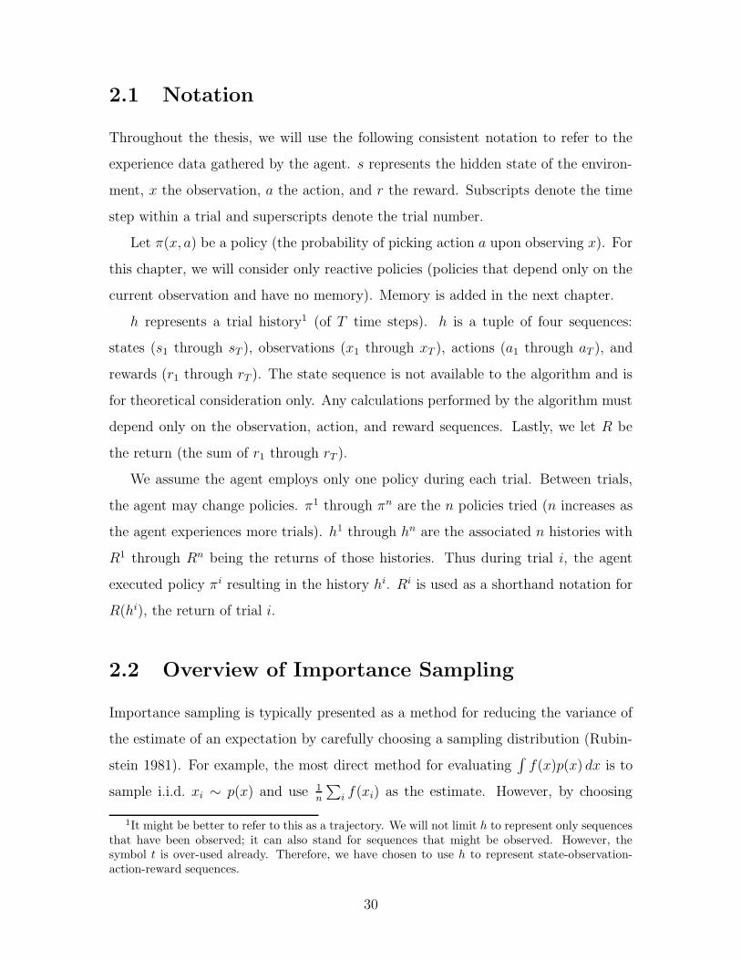
Figure 2-3: Left: Diagram of the left-right world. This world has eight states. Theagent receives no reward in the outlined states and one unit of reward each time itenters one of the solid states. The agent only observes whether it is in the left orright set of boxed states (a single bit of information). Each trial begins in the fourthstate from the left and lasts 100 time steps. Right: The true expected return as afunction of policy for this world. The optimal policy is at the point (0.4, 1) which isthe maximum of the plotted function.
constraints currently active. The constraint that all values sum to 1 is always active.
If the line search extends past one of the other boundary constraints (namely that each
value must be greater than some small positive constant), we active that constraint. If
the gradient points away from a constraint into the valid search region, we clear that
constraint. Each gradient calculated is projected onto the subspace defined by the
current active constraints. Any policy constructed during the line search is checked
against all constraints and projected into the valid region if it violates any constraints.
As a final performance improvement, we reduce the chance of being stuck in a
local minimum by starting the search at the previously sampled policy that has the
best estimated value. The estimated values of previously sampled policies can be
updated incrementally as each new trial ends.
42
normalized unnormalizedgreedy random greedy random
retu
rns
0 20 40 60 80 1000
10
20
30
40
50
60
70
80
90
trial number
retu
rn
0 20 40 60 80 1000
10
20
30
40
50
60
70
80
90
trial number
retu
rn
pol
icie
s
0 0.2 0.4 0.6 0.8 10
0.2
0.4
0.6
0.8
1
p(left | left)
p(le
ft | r
ight
)
0 0.2 0.4 0.6 0.8 10
0.2
0.4
0.6
0.8
1
p(left | left)
p(le
ft | r
ight
)
0 0.2 0.4 0.6 0.8 10
0.2
0.4
0.6
0.8
1
p(left | left)
p(le
ft | r
ight
)
0 0.2 0.4 0.6 0.8 10
0.2
0.4
0.6
0.8
1
p(left | left)
p(le
ft | r
ight
)
5iter
atio
ns
0
0.5
1
0
0.5
10
20
40
60
80
p(left | left)p(left | right)
retu
rn
0
0.5
1
0
0.5
10
20
40
60
80
p(left | left)p(left | right)
retu
rn
0
0.5
1
0
0.5
10
10
20
30
p(left | left)p(left | right)
retu
rn
0
0.5
1
0
0.5
10
50
100
150
p(left | left)p(left | right)
retu
rn
10iter
atio
ns
0
0.5
1
0
0.5
10
20
40
60
80
p(left | left)p(left | right)
retu
rn
0
0.5
1
0
0.5
10
20
40
60
80
p(left | left)p(left | right)
retu
rn
0
0.5
1
0
0.5
10
10
20
30
40
p(left | left)p(left | right)
retu
rn
0
0.5
1
0
0.5
10
20
40
60
80
p(left | left)p(left | right)
retu
rn
50iter
atio
ns
0
0.5
1
0
0.5
10
20
40
60
80
p(left | left)p(left | right)
retu
rn
0
0.5
1
0
0.5
10
20
40
60
80
p(left | left)p(left | right)
retu
rn
0
0.5
1
0
0.5
10
20
40
60
80
p(left | left)p(left | right)
retu
rn
0
0.5
1
0
0.5
10
100
200
300
400
p(left | left)p(left | right)
retu
rn
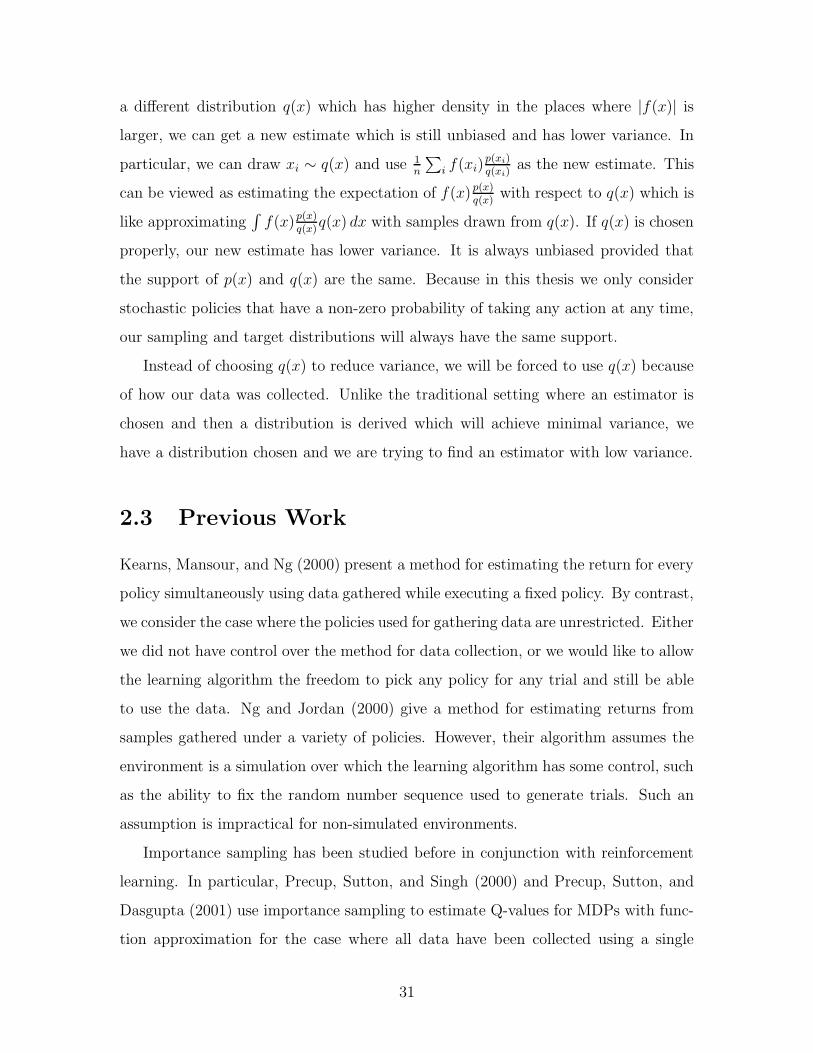
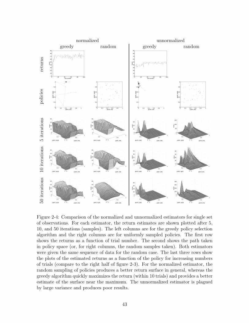
Figure 2-4: Comparison of the normalized and unnormalized estimators for single setof observations. For each estimator, the return estimates are shown plotted after 5,10, and 50 iterations (samples). The left columns are for the greedy policy selectionalgorithm and the right columns are for uniformly sampled policies. The first rowshows the returns as a function of trial number. The second shows the path takenin policy space (or, for right columns, the random samples taken). Both estimatorswere given the same sequence of data for the random case. The last three rows showthe plots of the estimated returns as a function of the policy for increasing numbersof trials (compare to the right half of figure 2-3). For the normalized estimator, therandom sampling of policies produces a better return surface in general, whereas thegreedy algorithm quickly maximizes the return (within 10 trials) and provides a betterestimate of the surface near the maximum. The unnormalized estimator is plaguedby large variance and produces poor results.
43

2.7 Results
Figure 2-3 shows a simple world for which policies can be described by two numbers
(the probability of going left when in the left half and the probability of going left when
in the right half) and the true expected return as a function of the policy. Figure 2-4
compares the normalized (equation 2.1) and unnormalized (equation 2.2) estimators
with both the greedy policy selection algorithm and random policy selection. We
feel this example is illustrative of the reasons that the normalized estimate works
much better on the problems we have tried. Its bias to observed returns works well
to smooth out the space. The estimator is willing to extrapolate to unseen regions
where the unnormalized estimator is not. This causes the greedy algorithm to explore
new areas of the policy space whereas the unnormalized estimator gets trapped in the
visited area under greedy exploration and does not successfully maximize the return
function.
44
Chapter 3
Extensions of Importance Sampling
“A liar should have a good memory.”
Institutiones Oratoriæ. iv. 2, 91.
Quintilian
We now move beyond reactive policies with action distributions specified as tables.
Although they are a good starting place, they are not always practical. Many domains
have too many observations (possibly a continuous space of observations) to make a
table possible. Additionally, a single instantaneous observation seldom captures all of
the necessary information. In this chapter we examine two extensions to the previous
algorithm: we allow for policies with memory and with function approximators. We
conclude the chapter with a pragmatic extension to the greedy search algorithm that
will prove useful for more noisy environments such as the one in chapter 5.
3.1 Memory
Memory is an important aspect to successful manipulation of the world. Many mem-
ory models have been tried in the past. In this thesis, we explore adding a fixed
memory space that can be read and modified as desired by the agent. In particular,
we use a finite-state controller model. In this model, the agent has an internal state
which, in addition to the observation, affects the action probabilities. This model
45

? ? ?
? ? ?
- -
- -
� �
R R R
R R
a1 a2 a3
m1 m2 m3
x1 x2 x3
s1 s2 s3
-time
Figure 3-1: Dependency graph for agent-world interaction with memory model. Thisis the same as the standard POMDP model except that the current action dependson previous observation through the current memory state.
has been studied before in conjunction with POMDP learning (Meuleau, Peshkin,
Kim, and Kaelbling 1999) but not with importance sampling which allows a greater
information gain.
3.1.1 Finite State Machine Model
At each time step, the agent reads the value of the memory along with the observation
and makes a choice about which action to take and the new value for the memory.
The policy now expands to the form π(x, m, a, m′) = p(a, m′|x, m), the probability of
picking action a and new memory state m′ given observation x and old memory state
m. The space of allowable memory states is fixed to a finite set, M. If |M| = 1,
there is only one memory state and the model reduces to the reactive policy class
of the previous chapter. The meanings of the memory states are not defined. It is
up to the RL algorithm to construct a policy which makes use of the memory in an
intelligent manner.
3.1.2 Memory Ratios
Let us factor the policy distribution, thereby limiting the class of policies realizable by
a fixed memory size slightly but making the model simpler. In particular we consider
46
an agent model where the agent’s policy has two parts: πa(x, m, a) and πm(x, m, m′).
The former is the probability of choosing action a given that the observation is x
and the internal memory is m. The latter is the probability of changing the inter-
nal memory to m′ given the observation is x and the internal memory is m. Thus
p(a, m′|x, m) = πa(x, m, a)πm(x, m, m′). By this factoring of the probability distribu-
tion of action-memory choices, we induce the dependency graph shown in figure 3-1.
If we let M be an arbitrary memory sequence m1, m2, . . . , mT , p(h|π) can be
written as
∑
M
p(h, M |π)
=∑
M
p(s0)p(m0)
T∏
t=0
(p(xt|st)πa(xt, mt, at)
πm(xt, mt, mt+1)p(st+1|st, at))
=
[
p(s0)T∏
t=0
p(xt|st)p(st+1|st, at)
]
[
∑
M
p(m0)
T∏
t=0
πa(xt, mt, at)πm(xt, mt, mt+1)
]
4= W (h)A(h, π) ,
once again splitting the probability into two parts: one for the world dynamics and
one for the agent dynamics. The A(h, π) term now involves a sum over all possible
memory sequences.
The beauty of this formulation is that it makes it explicit that the memory se-
quence does not affect the return except through the action sequence. In particular,
notice that the formula directly expresses that the probability of a history involves
marginalizing out the memory sequence. A memory sequence only indirectly affects
the return through its effect on the action sequence. This explicit modeling of the
memory dynamics allows a single trial’s experience to affect every policy that could
have produced the action sequence without considering the memory sequence that
occurred. Note that the history does not include the memory sequence and the mem-
47
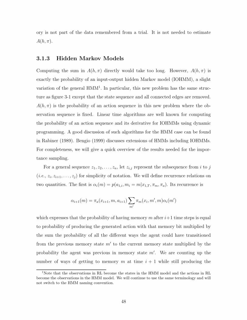
ory is not part of the data remembered from a trial. It is not needed to estimate
A(h, π).
3.1.3 Hidden Markov Models
Computing the sum in A(h, π) directly would take too long. However, A(h, π) is
exactly the probability of an input-output hidden Markov model (IOHMM), a slight
variation of the general HMM1. In particular, this new problem has the same struc-
ture as figure 3-1 except that the state sequence and all connected edges are removed.
A(h, π) is the probability of an action sequence in this new problem where the ob-
servation sequence is fixed. Linear time algorithms are well known for computing
the probability of an action sequence and its derivative for IOHMMs using dynamic
programming. A good discussion of such algorithms for the HMM case can be found
in Rabiner (1989). Bengio (1999) discusses extensions of HMMs including IOHMMs.
For completeness, we will give a quick overview of the results needed for the impor-
tance sampling.
For a general sequence z1, z2, . . . , zn, let zi,j represent the subsequence from i to j
(i.e., zi, zi+1, . . . , zj) for simplicity of notation. We will define recurrence relations on
two quantities. The first is αi(m) = p(a1,i, mi = m|x1,T , πm, πa). Its recurrence is
αi+1(m) = πa(xi+1, m, ai+1)∑
m′
πm(xi, m′, m)αi(m
′)
which expresses that the probability of having memory m after i+1 time steps is equal
to probability of producing the generated action with that memory bit multiplied by
the sum the probability of all the different ways the agent could have transitioned
from the previous memory state m′ to the current memory state multiplied by the
probability the agent was previous in memory state m′. We are counting up the
number of ways of getting to memory m at time i + 1 while still producing the
1Note that the observations in RL become the states in the HMM model and the actions in RLbecome the observations in the HMM model. We will continue to use the same terminology and willnot switch to the HMM naming convention.
48
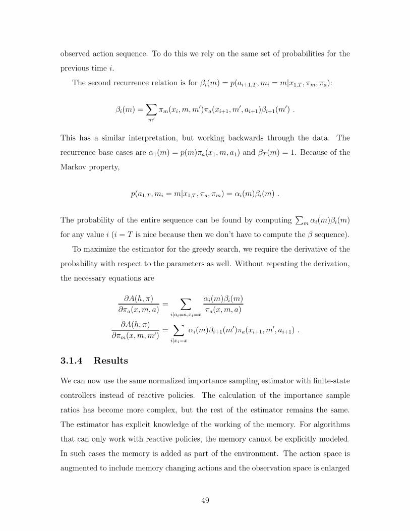
observed action sequence. To do this we rely on the same set of probabilities for the
previous time i.
The second recurrence relation is for βi(m) = p(ai+1,T , mi = m|x1,T , πm, πa):
βi(m) =∑
m′
πm(xi, m, m′)πa(xi+1, m′, ai+1)βi+1(m
′) .
This has a similar interpretation, but working backwards through the data. The
recurrence base cases are α1(m) = p(m)πa(x1, m, a1) and βT (m) = 1. Because of the
Markov property,
p(a1,T , mi = m|x1,T , πa, πm) = αi(m)βi(m) .
The probability of the entire sequence can be found by computing∑
m αi(m)βi(m)
for any value i (i = T is nice because then we don’t have to compute the β sequence).
To maximize the estimator for the greedy search, we require the derivative of the
probability with respect to the parameters as well. Without repeating the derivation,
the necessary equations are
∂A(h, π)
∂πa(x, m, a)=
∑
i|ai=a,xi=x
αi(m)βi(m)
πa(x, m, a)
∂A(h, π)
∂πm(x, m, m′)=∑
i|xi=x
αi(m)βi+1(m′)πa(xi+1, m
′, ai+1) .
3.1.4 Results
We can now use the same normalized importance sampling estimator with finite-state
controllers instead of reactive policies. The calculation of the importance sample
ratios has become more complex, but the rest of the estimator remains the same.
The estimator has explicit knowledge of the working of the memory. For algorithms
that can only work with reactive policies, the memory cannot be explicitly modeled.
In such cases the memory is added as part of the environment. The action space is
augmented to include memory changing actions and the observation space is enlarged
49
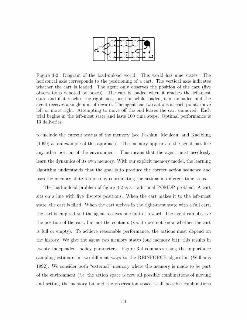
j j j
j j j
Y
Y
Y
Y
Y
�
:9
I:
Y
�
Figure 3-2: Diagram of the load-unload world. This world has nine states. Thehorizontal axis corresponds to the positioning of a cart. The vertical axis indicateswhether the cart is loaded. The agent only observes the position of the cart (fiveobservations denoted by boxes). The cart is loaded when it reaches the left-moststate and if it reaches the right-most position while loaded, it is unloaded and theagent receives a single unit of reward. The agent has two actions at each point: moveleft or move right. Attempting to move off the end leaves the cart unmoved. Eachtrial begins in the left-most state and lasts 100 time steps. Optimal performance is13 deliveries.
to include the current status of the memory (see Peshkin, Meuleau, and Kaelbling
(1999) as an example of this approach). The memory appears to the agent just like
any other portion of the environment. This means that the agent must needlessly
learn the dynamics of its own memory. With our explicit memory model, the learning
algorithm understands that the goal is to produce the correct action sequence and
uses the memory state to do so by coordinating the actions in different time steps.
The load-unload problem of figure 3-2 is a traditional POMDP problem. A cart
sits on a line with five discrete positions. When the cart makes it to the left-most
state, the cart is filled. When the cart arrives in the right-most state with a full cart,
the cart is emptied and the agent receives one unit of reward. The agent can observe
the position of the cart, but not the contents (i.e. it does not know whether the cart
is full or empty). To achieve reasonable performance, the actions must depend on
the history. We give the agent two memory states (one memory bit); this results in
twenty independent policy parameters. Figure 3-4 compares using the importance
sampling estimate in two different ways to the REINFORCE algorithm (Williams
1992). We consider both “external” memory where the memory is made to be part
of the environment (i.e. the action space is now all possible combinations of moving
and setting the memory bit and the observation space is all possible combinations
50
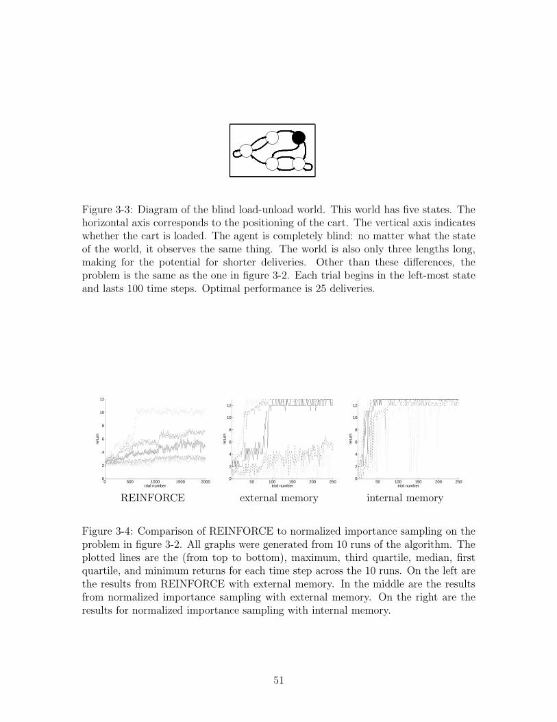
j
j
Y
��
Y
:9
I:
Figure 3-3: Diagram of the blind load-unload world. This world has five states. Thehorizontal axis corresponds to the positioning of the cart. The vertical axis indicateswhether the cart is loaded. The agent is completely blind: no matter what the stateof the world, it observes the same thing. The world is also only three lengths long,making for the potential for shorter deliveries. Other than these differences, theproblem is the same as the one in figure 3-2. Each trial begins in the left-most stateand lasts 100 time steps. Optimal performance is 25 deliveries.
0 500 1000 1500 20000
2
4
6
8
10
12
trial number
retu
rn
50 100 150 200 2500
2
4
6
8
10
12
trial number
retu
rn
50 100 150 200 2500
2
4
6
8
10
12
trial number
retu
rn
REINFORCE external memory internal memory
Figure 3-4: Comparison of REINFORCE to normalized importance sampling on theproblem in figure 3-2. All graphs were generated from 10 runs of the algorithm. Theplotted lines are the (from top to bottom), maximum, third quartile, median, firstquartile, and minimum returns for each time step across the 10 runs. On the left arethe results from REINFORCE with external memory. In the middle are the resultsfrom normalized importance sampling with external memory. On the right are theresults for normalized importance sampling with internal memory.
51

50 100 150 200 250 3000
5
10
15
20
25
trial number
retu
rn
50 100 150 200 250 3000
5
10
15
20
25
trial number
retu
rn
external memory internal memory
Figure 3-5: Comparison of placing the memory bits externally as part of the environ-ment to modeling them explicitly as an internal part of the agent for the problem infigure 3-3. Both graphs were generated from 10 runs of the normalized importancesampling algorithm. The plotted lines are the (from top to bottom), maximum, thirdquartile, median, first quartile, and minimum returns for each time step across the10 runs.
of position and memory state) and “internal” memory where the memory model is
explicit as described in this chapter. REINFORCE can only use external memory.
On the left is the result of running the REINFORCE algorithm with an external
memory representation. In the middle is the result of using external memory with the
normalized importance sampling estimator. And, on the right is the result of using
internal memory with normalize importance sampling. The REINFORCE results
are for the best settings for the step size schedule and the bias term. Yet, it still
frequently gets stuck in local minima and only 2 out of the 10 experiments manage
to converge to a near-optimal solution (in roughly 500 trials). By comparison, the
importance sampling algorithm usually converges in approximately 100 trials with
external memory and almost always converges within 50 trials with internal memory.
To consider a more drastic example, we constructed a blind load-unload problem,
as shown in figure 3-3. In this case, we give the agent four memory states (two mem-
ory bits). Figure 3-5 compares the result of internal and external memory for the
normalized importance sampling estimate. Again, we see a clear gain by explicitly
modeling the memory dynamics. With an increase in the importance of memory, we
see an increase in the difference between external and internal memory representa-
tions. Whereas figure 3-4 demonstrates a 2-fold speed-up, figure 3-5 demonstrates a
52
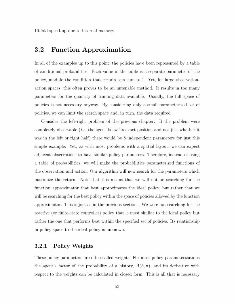
10-fold speed-up due to internal memory.
3.2 Function Approximation
In all of the examples up to this point, the policies have been represented by a table
of conditional probabilities. Each value in the table is a separate parameter of the
policy, modulo the condition that certain sets sum to 1. Yet, for large observation-
action spaces, this often proves to be an untenable method. It results in too many
parameters for the quantity of training data available. Usually, the full space of
policies is not necessary anyway. By considering only a small parameterized set of
policies, we can limit the search space and, in turn, the data required.
Consider the left-right problem of the previous chapter. If the problem were
completely observable (i.e. the agent knew its exact position and not just whether it
was in the left or right half) there would be 8 independent parameters for just this
simple example. Yet, as with most problems with a spatial layout, we can expect
adjacent observations to have similar policy parameters. Therefore, instead of using
a table of probabilities, we will make the probabilities parameterized functions of
the observation and action. Our algorithm will now search for the parameters which
maximize the return. Note that this means that we will not be searching for the
function approximator that best approximates the ideal policy, but rather that we
will be searching for the best policy within the space of policies allowed by the function
approximator. This is just as in the previous sections. We were not searching for the
reactive (or finite-state controller) policy that is most similar to the ideal policy but
rather the one that performs best within the specified set of policies. Its relationship
in policy space to the ideal policy is unknown.
3.2.1 Policy Weights
These policy parameters are often called weights. For most policy parameterizations
the agent’s factor of the probability of a history, A(h, π), and its derivative with
respect to the weights can be calculated in closed form. This is all that is necessary
53
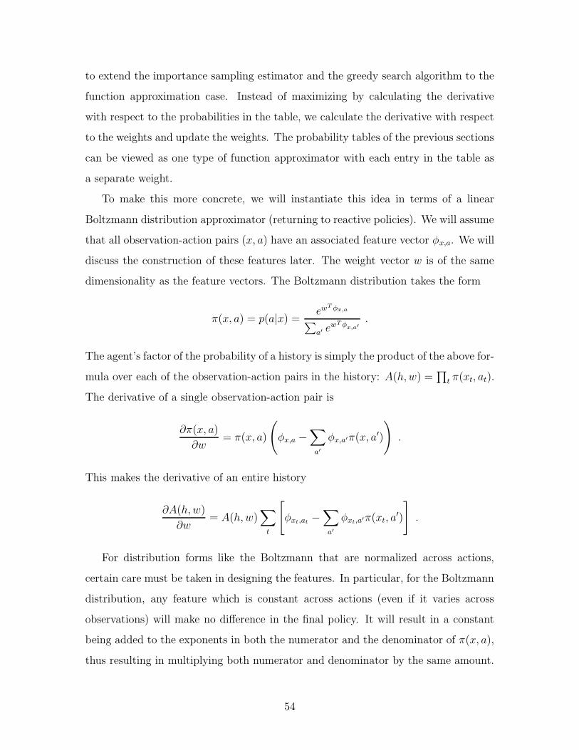
to extend the importance sampling estimator and the greedy search algorithm to the
function approximation case. Instead of maximizing by calculating the derivative
with respect to the probabilities in the table, we calculate the derivative with respect
to the weights and update the weights. The probability tables of the previous sections
can be viewed as one type of function approximator with each entry in the table as
a separate weight.
To make this more concrete, we will instantiate this idea in terms of a linear
Boltzmann distribution approximator (returning to reactive policies). We will assume
that all observation-action pairs (x, a) have an associated feature vector φx,a. We will
discuss the construction of these features later. The weight vector w is of the same
dimensionality as the feature vectors. The Boltzmann distribution takes the form
π(x, a) = p(a|x) =ewT φx,a
∑
a′ ewT φx,a′
.
The agent’s factor of the probability of a history is simply the product of the above for-
mula over each of the observation-action pairs in the history: A(h, w) =∏
t π(xt, at).
The derivative of a single observation-action pair is
∂π(x, a)
∂w= π(x, a)
(
φx,a −∑
a′
φx,a′π(x, a′)
)
.
This makes the derivative of an entire history
∂A(h, w)
∂w= A(h, w)
∑
t
[
φxt,at−∑
a′
φxt,a′π(xt, a′)
]
.
For distribution forms like the Boltzmann that are normalized across actions,
certain care must be taken in designing the features. In particular, for the Boltzmann
distribution, any feature which is constant across actions (even if it varies across
observations) will make no difference in the final policy. It will result in a constant
being added to the exponents in both the numerator and the denominator of π(x, a),
thus resulting in multiplying both numerator and denominator by the same amount.
54
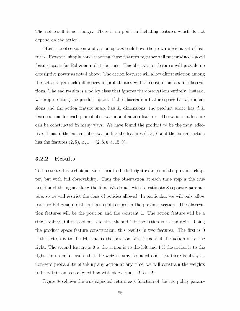
The net result is no change. There is no point in including features which do not
depend on the action.
Often the observation and action spaces each have their own obvious set of fea-
tures. However, simply concatenating those features together will not produce a good
feature space for Boltzmann distributions. The observation features will provide no
descriptive power as noted above. The action features will allow differentiation among
the actions, yet such differences in probabilities will be constant across all observa-
tions. The end results is a policy class that ignores the observations entirely. Instead,
we propose using the product space. If the observation feature space has do dimen-
sions and the action feature space has da dimensions, the product space has doda
features: one for each pair of observation and action features. The value of a feature
can be constructed in many ways. We have found the product to be the most effec-
tive. Thus, if the current observation has the features (1, 3, 0) and the current action
has the features (2, 5), φx,a = (2, 6, 0, 5, 15, 0).
3.2.2 Results
To illustrate this technique, we return to the left-right example of the previous chap-
ter, but with full observability. Thus the observation at each time step is the true
position of the agent along the line. We do not wish to estimate 8 separate parame-
ters, so we will restrict the class of policies allowed. In particular, we will only allow
reactive Boltzmann distributions as described in the previous section. The observa-
tion features will be the position and the constant 1. The action feature will be a
single value: 0 if the action is to the left and 1 if the action is to the right. Using
the product space feature construction, this results in two features. The first is 0
if the action is to the left and is the position of the agent if the action is to the
right. The second feature is 0 is the action is to the left and 1 if the action is to the
right. In order to insure that the weights stay bounded and that there is always a
non-zero probability of taking any action at any time, we will constrain the weights
to lie within an axis-aligned box with sides from −2 to +2.
Figure 3-6 shows the true expected return as a function of the two policy param-
55
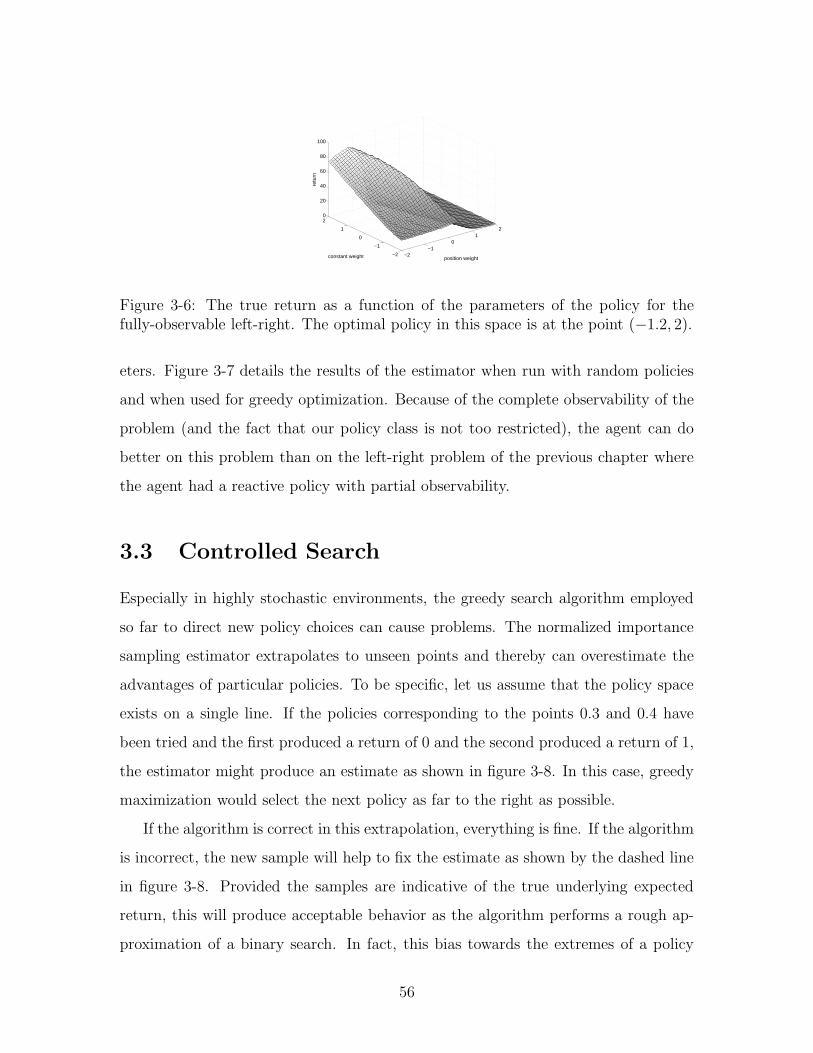
−2−1
01
2
−2
−1
0
1
20
20
40
60
80
100
position weightconstant weight
retu
rnFigure 3-6: The true return as a function of the parameters of the policy for thefully-observable left-right. The optimal policy in this space is at the point (−1.2, 2).
eters. Figure 3-7 details the results of the estimator when run with random policies
and when used for greedy optimization. Because of the complete observability of the
problem (and the fact that our policy class is not too restricted), the agent can do
better on this problem than on the left-right problem of the previous chapter where
the agent had a reactive policy with partial observability.
3.3 Controlled Search
Especially in highly stochastic environments, the greedy search algorithm employed
so far to direct new policy choices can cause problems. The normalized importance
sampling estimator extrapolates to unseen points and thereby can overestimate the
advantages of particular policies. To be specific, let us assume that the policy space
exists on a single line. If the policies corresponding to the points 0.3 and 0.4 have
been tried and the first produced a return of 0 and the second produced a return of 1,
the estimator might produce an estimate as shown in figure 3-8. In this case, greedy
maximization would select the next policy as far to the right as possible.
If the algorithm is correct in this extrapolation, everything is fine. If the algorithm
is incorrect, the new sample will help to fix the estimate as shown by the dashed line
in figure 3-8. Provided the samples are indicative of the true underlying expected
return, this will produce acceptable behavior as the algorithm performs a rough ap-
proximation of a binary search. In fact, this bias towards the extremes of a policy
56
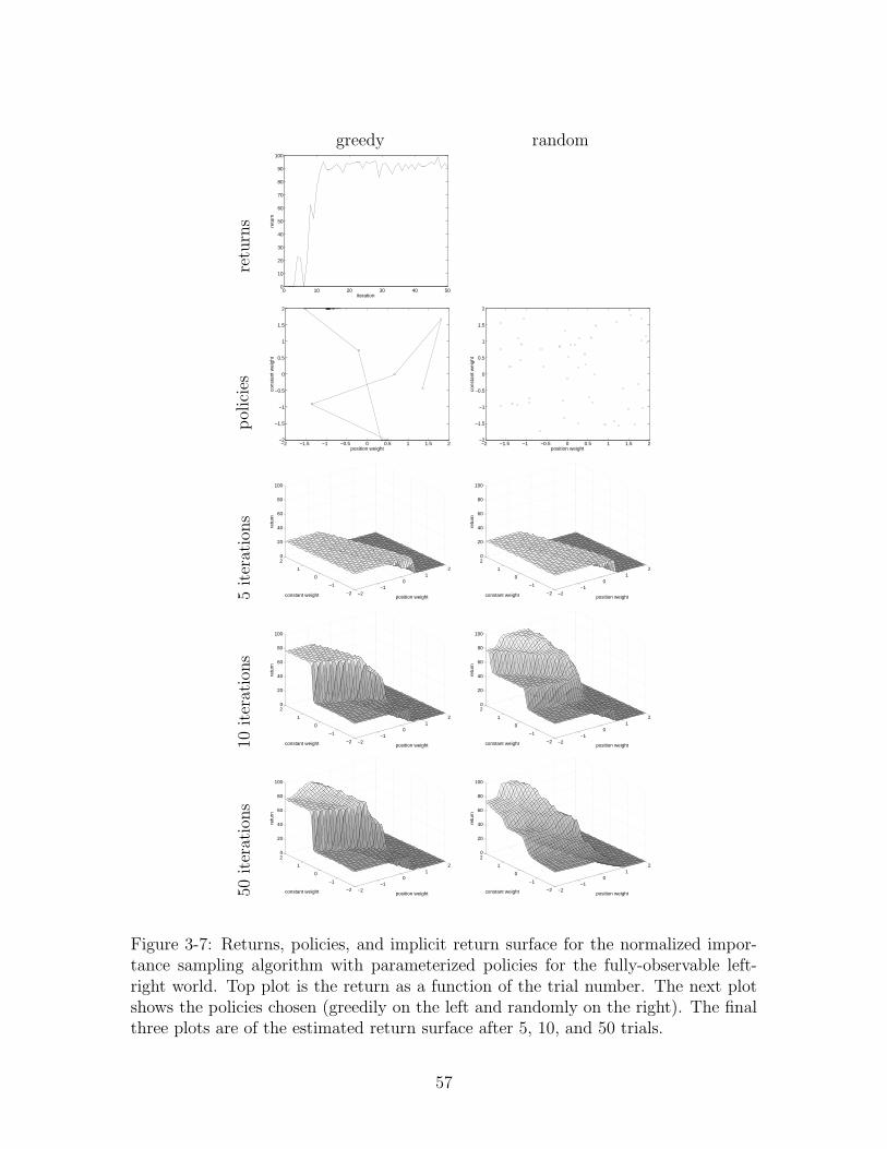
greedy random
retu
rns
0 10 20 30 40 500
10
20
30
40
50
60
70
80
90
100
iteration
retu
rn
pol
icie
s
−2 −1.5 −1 −0.5 0 0.5 1 1.5 2−2
−1.5
−1
−0.5
0
0.5
1
1.5
2
position weight
cons
tant
wei
ght
−2 −1.5 −1 −0.5 0 0.5 1 1.5 2−2
−1.5
−1
−0.5
0
0.5
1
1.5
2
position weight
cons
tant
wei
ght
5iter
atio
ns
−2−1
01
2
−2
−1
0
1
20
20
40
60
80
100
position weightconstant weight
retu
rn
−2−1
01
2
−2
−1
0
1
20
20
40
60
80
100
position weightconstant weight
retu
rn
10iter
atio
ns
−2−1
01
2
−2
−1
0
1
20
20
40
60
80
100
position weightconstant weight
retu
rn
−2−1
01
2
−2
−1
0
1
20
20
40
60
80
100
position weightconstant weight
retu
rn
50iter
atio
ns
−2−1
01
2
−2
−1
0
1
20
20
40
60
80
100
position weightconstant weight
retu
rn
−2−1
01
2
−2
−1
0
1
20
20
40
60
80
100
position weightconstant weight
retu
rn
Figure 3-7: Returns, policies, and implicit return surface for the normalized impor-tance sampling algorithm with parameterized policies for the fully-observable left-right world. Top plot is the return as a function of the trial number. The next plotshows the policies chosen (greedily on the left and randomly on the right). The finalthree plots are of the estimated return surface after 5, 10, and 50 trials.
57
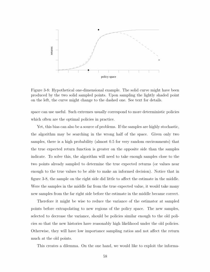
retu
rns
policy space
Figure 3-8: Hypothetical one-dimensional example. The solid curve might have beenproduced by the two solid sampled points. Upon sampling the lightly shaded pointon the left, the curve might change to the dashed one. See text for details.
space can use useful. Such extremes usually correspond to more deterministic policies
which often are the optimal policies in practice.
Yet, this bias can also be a source of problems. If the samples are highly stochastic,
the algorithm may be searching in the wrong half of the space. Given only two
samples, there is a high probability (almost 0.5 for very random environments) that
the true expected return function is greater on the opposite side than the samples
indicate. To solve this, the algorithm will need to take enough samples close to the
two points already sampled to determine the true expected returns (or values near
enough to the true values to be able to make an informed decision). Notice that in
figure 3-8, the sample on the right side did little to affect the estimate in the middle.
Were the samples in the middle far from the true expected value, it would take many
new samples from the far right side before the estimate in the middle became correct.
Therefore it might be wise to reduce the variance of the estimator at sampled
points before extrapolating to new regions of the policy space. The new samples,
selected to decrease the variance, should be policies similar enough to the old poli-
cies so that the new histories have reasonably high likelihood under the old policies.
Otherwise, they will have low importance sampling ratios and not affect the return
much at the old points.
This creates a dilemma. On the one hand, we would like to exploit the informa-
58
tion gained from the original two samples and jump to the current maximum of the
estimated return function. Yet, we might also like to verify the information gained
before taking such a large jump. This is an example of the exploration-exploitation
dilemma mentioned in chapter 1. In higher-dimensional policy spaces the problem
becomes more pronounced. Search in the “wrong” half of the space is a bigger penalty
because of the greater size of that half.
The most obvious solution is to take multiple samples from each policy chosen:
instead of changing the policy by maximizing every trial, we could modify the algo-
rithm to only change the policy every k trials. However this can be wasteful. If a
new chosen policy is near other samples, its variance may already be small. Forcing
multiple samples from this new point would be needless. In general, it would seem
better to simply limit the maximization routine to stay within the part of policy space
in which we are confident of our estimated return. This insures that any new chosen
policy will already have low variance due to its proximity to previous samples.
We have not yet developed an entirely principled way of achieving this. Techniques
in experiment design like response surfaces (Box and Draper 1987) have found ways
to deal with the variance in the environment. However, such methods, as mentioned
in the introduction, are more general than reinforcement learning. We would like
to exploit our knowledge about the environment dynamics inherent to reinforcement
learning problems. While we have a variance formula for the estimator (shown in
the previous chapter and detailed in the appendix), this formula requires specific
knowledge of the environment which the algorithm does not have. We have not found
a good method for estimating the needed probability distributions. Instead, we take
a more pragmatic view.
The source of variance in the estimate comes from misestimating the probabilities
of histories and a sparse sampling of the history space. Thus, in the estimator
∑
i Ri p(hi|π)∑
j p(hi|πj)∑
ip(hi|π)
∑
j p(hi|πj)
,
the returns, Ri, are deterministic whereas the weights associated with them are the
59

source of the error. In fact, there is an implied 0 weight to all histories we have
not yet sampled. As mentioned above, this error is difficult to compute, so instead,
we will assume the reverse: the weights are correct and fixed, and the returns are
random variables. Thus, our estimator is the linear combination of random variables.
If we furthermore assume that all of the returns have the same variance σ2 and let
win(π) be the normalized weight for return Ri, then the variance of our estimator is
σ2∑
i(win(π))2. So, while the absolute magnitude of the variance cannot be deter-
mined (σ is unknown), we can determine the relative variances among the estimates
for difference policies.
To use this knowledge, we limit the range of the policy search to areas where∑
i(win(π)2) is less than a threshold θ. If no such regions exist, we reuse the sampled
policy with the best estimated value instead thereby decreasing the variance near that
sample. θ is application dependent and must be set on a case-by-case basis. Although
it is unfortunate to add a tuning parameter to the algorithm, we have found it to be
invaluable (despite the lack of theoretical justification) for achieving convergence in
reasonable time. All of the results in chapter 5 use this method.
60

Chapter 4
Balancing Multiple Goals
“I do perceive here a divided duty.”
Othello. act i. sc 3.
William Shakespeare
The importance sampling methods of the previous chapters estimate the entire
return surface. Therefore, they can be used not only to find the policy with the
maximum return, but they can also be used to find other important or interesting
policies. In this chapter, we develop two methods for balancing multiple objectives
simultaneously that utilize the complete return surface characterization.
Others have previously considered the case of multiple objectives. In particular,
Gabor, Kalmar, and Szepesvari (1998) describe the notion of partial orderings over
solutions and develop a framework based on MDPs. Geibel (2001) applies this idea
to balancing expected return and risk. In section 4.2, we use these ideas but work
with POMDP models and extend the estimators of the previous chapters.
For section 4.3 we take a different approach. Instead of attempting to optimize all
objectives simultaneously, we fix a minimum necessary performance with regard to
one or more of the objectives and then optimize the rest of the objectives as before.
This makes different guarantees on the performance of the resulting policy. Each
technique is applicable to a different type of objective.
This chapter differs from our previous work (Shelton 2001) in that it does not
61

take a game theoretic approach to balancing. We achieve the same results but can
guarantee qualities of performance that were not possible with the our prior method.
4.1 Rewards as Goals
Many agents have multiple objectives. The pedagogical example from robotics is an
office service robot. The robot needs to deliver mail to employees’ offices, stock the
printer with paper, and keep its battery charged. Designing a return function for
each of these tasks independently is simple. However, designing a return function
that balances each of these tasks can be more difficult.
Consider the case of mail delivery and paper restocking. We might give the agent
one unit of reward each time mail is delivered or paper is restocked. If we only
consider the mail delivery, the agent does the right thing: it delivers mail as often as
possible. The same is true of the paper restocking. However, put together, the agent
will only fulfill one of its duties: whichever is easier or quicker. There is no sense in
restocking the paper at all if mail delivery is faster and results in the same reward.
We can try to solve this by reweighting or discounting the rewards. Yet, this
does not solve the real problem. These rewards are difficult to combine because they
were not designed to be combined. Each specifies the successfulness of completing a
particular goal. However, their sum (or any other fixed combination) has no guarantee
to represent a desirable objective on its own.
Note that in some cases separate goals can be combined. For instance, a store
may wish to both sell as many products as possible and charge the highest price.
However, there is a clear way of combining the two objectives. The overall goal is to
maximize profits for which the proper objective is the multiplication of the price and
the number sold (ignoring fixed costs). In this chapter, we are interested in situations
for which such a combination is unknown or impossible.
Such an example naturally arises when there are multiple users of a system. Each
user might express his or her content with the system through rewards. Optimizing
the total content of the users is not as simple as optimizing the sum of their rewards.
62

One user might decide to reward twice as often or with twice the force as another.
That should not necessarily result in this user gaining twice the control over the
behavior of the agent. Limiting the amount of reward possible from a given user does
not solve the problem; it merely deafens the agent’s ability to correctly distinguish
the preferences of its users.
Whether each reward represents an objective or a user’s desire, we will call each
separate reward signal a source. We are considering problem for which rewards are
comparable within the same source, but are not comparable across sources.
4.1.1 Related Work
The same problem also arises in the context of social choice theory. We recommend
Resnik (1987) as a good introduction to the subject. In a social choice problem, each
objective corresponds to a citizen and the goal is to pick a single global policy based
on all of the citizens’ individual preferences. Most of the work does not promote
direct calculation or single unique solutions. The necessary computations to achieve
the answer are, for our domain, intractable and for most situations do not yield a
single solution, but a set of possible solutions with no principled way of selecting
among them.
The most promising areas of social choice theory deal with utility functions. Util-
ity functions directly correspond to the expected returns in our application. How-
ever, these methods assume utilities can be compared across individuals (or reward
sources). We are unwilling to make this assumption. For our problem, we would like
to be able to design each reward function for each objective independently without
consideration as to how it will dovetail with the other reward functions. Furthermore,
each reward source might be associated with an individual user in which case it cer-
tainly undesirable to assume that the rewards provided by one user can be directly
compared against those of another user. Personal style may cause two people with
the same preferences to manifest them in different reward techniques.
Even in social choice theory, the notion of comparable utilities is questionable. It is
uncertain how to elicit true comparable utilities from people. The area of mechanism
63
design or implementation theory (Mas-Collel, Whinston, and Green 1995; Green and
Laffont 1979) deals directly with this problem, but in the context of an extensible
universally desired good, money. Without the ability to pay or charge the citizens (or
objectives), we cannot employ the algorithms and methods from that area of research.
4.1.2 Notation
We modify the standard POMDP framework slightly to include multiple sources. We
keep the state space, action space, and observation spaces as well as the starting state,
state transition, and observation probabilities the same as in the regular definition.
However, we modify the reward function. Although still a deterministic function of the
state, the reward function is now a vector quantity with each dimension representing
the reward from a different source.
The goal of the agent is no longer to optimize a scalar quantity but rather to
simultaneously optimize all of the expected returns (each return is the sum of one
dimension of the reward vector). In some special cases it may be possible to maximize
all of the returns simultaneously. However, in general, a trade-off must be made
among the sources. For this problem, there is no single correct or optimal solution.
We propose two solution methods that each have different solution guarantees.
For notation, we will let R(π) be the estimate expected return for following policy
π. R(π) is therefore a vector of length m, the number of reward sources. Ri(π) will
denote the ith element of that vector. Each element is estimated individually with
its own importance sampling estimator.
4.2 Policy Equilibria
A reward function implies an ordering over policies. In particular, we can infer that
πA is preferred to πB if and only if R(πA) > R(πB). Many reward functions are
consistent with a single policy preference ordering. We define reward restructuring as
any change to the reward function that does not change the policy preference ordering.
We would like to develop an algorithm that is insensitive to reward restructuring for
64
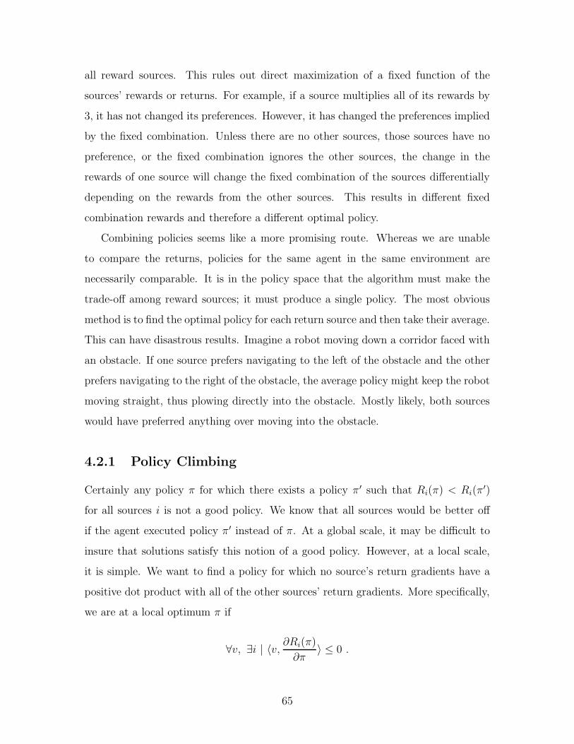
all reward sources. This rules out direct maximization of a fixed function of the
sources’ rewards or returns. For example, if a source multiplies all of its rewards by
3, it has not changed its preferences. However, it has changed the preferences implied
by the fixed combination. Unless there are no other sources, those sources have no
preference, or the fixed combination ignores the other sources, the change in the
rewards of one source will change the fixed combination of the sources differentially
depending on the rewards from the other sources. This results in different fixed
combination rewards and therefore a different optimal policy.
Combining policies seems like a more promising route. Whereas we are unable
to compare the returns, policies for the same agent in the same environment are
necessarily comparable. It is in the policy space that the algorithm must make the
trade-off among reward sources; it must produce a single policy. The most obvious
method is to find the optimal policy for each return source and then take their average.
This can have disastrous results. Imagine a robot moving down a corridor faced with
an obstacle. If one source prefers navigating to the left of the obstacle and the other
prefers navigating to the right of the obstacle, the average policy might keep the robot
moving straight, thus plowing directly into the obstacle. Mostly likely, both sources
would have preferred anything over moving into the obstacle.
4.2.1 Policy Climbing
Certainly any policy π for which there exists a policy π ′ such that Ri(π) < Ri(π′)
for all sources i is not a good policy. We know that all sources would be better off
if the agent executed policy π′ instead of π. At a global scale, it may be difficult to
insure that solutions satisfy this notion of a good policy. However, at a local scale,
it is simple. We want to find a policy for which no source’s return gradients have a
positive dot product with all of the other sources’ return gradients. More specifically,
we are at a local optimum π if
∀v, ∃i | 〈v,∂Ri(π)
∂π〉 ≤ 0 .
65
This implies that at such an optimum no instantaneous change, v, in the policy will
produce a new policy that is not worse for at least one of the return sources.
The obvious search algorithm is therefore to begin with a policy and continue to
climb all return surfaces at the same time by picking changes to the policy that have
a positive dot product with all return derivatives. There are two main specifications
left in such an algorithm. First, which direction, of the many with non-negative dot
product with all gradients, should be selected for each step. And second, how should
the initial policy should be selected.
To pick a step direction, let ∆i be the gradient of the return of source i with respect
to the policy parameters evaluated at the current policy. We can then calculate ∆i,
the normalized direction with a non-negative dot product with all of the gradients
which has the highest dot product with ∆i. ∆i is the vector on the unit sphere
which has the largest dot product with ∆i while still satisfying the constraint of non-
negative gain for all of the returns. Any vector ∆ that is a convex combination of
∆1, ∆2, . . . , ∆m satisfies all of the non-negative dot product constraints. We fix a set
of convex combination coefficients based on the relative importance of the various
return sources. Note that because ∆i is normalized, the magnitude of change in the
returns does not matter; only the local relative preferences matter.
Picking the initial policy at which to begin the climb is important. In particular,
this choice specifies the performance guarantee of the final policy: the final policy
will have returns no worse than the initial policy. For this reason, we pick the initial
policy to be a mixture of the best policies for each of the return sources individually.
A mixture policy is a policy that, at t = 0, randomly picks one of its component
subpolicies and then executes that single subpolicy for the entire trial. Thus, the
expected return of a mixture policy is a weighted average of the expected returns
of its components where the weights are the same as the weights on the mixture’s
subpolicy. The weights of the mixture can be selected to be the same as the weights
of the direction combination or different depending on the type of solution desired.
The joint maximization algorithm is shown in figure 4-1. Step 1 is accomplished
by the maximization detailed in the previous chapters. The gradient in step 3 is with
66

Input: R1(π), R2(π), . . . , Rm(π)Output: πParameters: (α1, α2, . . . , αm), (β1, β2, . . . , βm), ηConstraints:
∑
i αi = 1,∑
i βi = 1
1. Using the single source maximization procedure, for all sources i, let θi be theparameters of the maximization of Ri over all policies in the input policy class.
2. Let Φ be the parameters of a mixture policy with mixture weights α1, α2, . . . , αm
and subpolicies with parameters θ1, θ2, . . . , θm.
3. For all sources i, let ∆i be the gradient of Ri evaluated at the mixture policywith parameters Φ.
4. For all sources i, let ∆i be the vector in gradient space with the largest dotproduct with ∆i subject to the constraints that the magnitude of ∆i be 1 and∆i ·∆j ≥ 0 for all sources j.
5. If ∆i does not exist for any source i, quit and return the mixture policy Φ.Otherwise, let ∆ =
∑
i αi∆i
6. If |∆| = 0 quit and return the mixture policy Φ.
7. Normalize ∆ to be unit length.
8. Let Φ′ = Φ + η∆.
9. If Ri(Φ′) ≥ Ri(Φ) for all sources i, let Φ = Φ′ and jump back to step 3.
10. Let η = η/2.If η is too small, return the mixture policy ΦOtherwise, jump back to step 8.
Figure 4-1: Joint maximization search algorithm
67
respect to all parameters (all subpolicy parameters and the mixture parameters).
The constraint satisfaction program of step 4 in general can be difficult. However,
with a small number of constraints, it can be solved quickly by searching all possible
combinations of active constraints. The α-values are the starting policy combination
coefficients. They specify the relative importance of the sources in selecting the start-
ing policy; the starting policy dictates the performance guarantees for the algorithm.
The β-values are the gradient combination coefficients. While hill-climbing, they
specify the relative importance of increasing each source’s return. η is the maximum
step size.
A number of interesting parameter combinations are possible. If αi = βi for all
sources i, then these values represent the global relative importance of maximizing
each source. If βi = 0 for some i, then the algorithm does not maximize Ri but rather
just enforces the constraint Ri(π) ≥∑
j αj maxπ′ Rj(π′), that the return from this
source be no worse than the return from the mixture of individually optimal policies.
4.2.2 Algorithm
Just as we previously took a maximization procedure and turned it into a greedy
RL algorithm, we can do the same with the procedure of figure 4-1. Before each
trial, the agent runs the joint maximization algorithm to find a new policy. The
joint maximization procedure is given the current estimated return functions based
on the data collected so far. These functions may incorporate the controlled search
method from the previous chapter and limit the valid area of search to those policies
with small estimated variance. The agent executes the policy returned by the joint
maximization procedure and then adds it and the observed history to its data. Using
the new data set, it reiterates for the next trial.
4.2.3 Results
Figure 4-2 shows a test world for comparing the joint maximization method of the
previous section to other techniques. Note that while source 1 would prefer the left
68

0 0 0
0 0 0
0
0
0
1
1
0
.75
.75
j j j
Y Y Y
U
UKI
s+
jK K
Figure 4-2: Diagram of the cooperate world. The world state is fully observable. Thecenter state has three choices (each a different “arm”). Each middle state of an armhas three choices: go back, stay in the center, move to the end. From the end statesthe agent has no choice but to return to the center. The top number in a state isthe reward from source 1 upon entering the state. The bottom number is the rewardfrom source 2. Trials last for 20 time steps.
arm of the POMDP and source 2 would prefer the right arm, the lower arm is an
acceptable compromise which is better than randomly picking between the left and
right.
Figure 4-3 shows the results of running the joint maximization procedure of this
chapter against two other possible methods. The “mixture” procedure is to find the
optimal policies for each source independently (using the importance sampling from
the previous chapters) and then compose a final policy that is a weighted mixture
policy of the found optimal policies. The “sum maximization” procedure is to max-
imize the weighted sum of returns using the importance sampling from the previous
chapters. For the joint maximization, we let αi = βi.
The first important thing to notice is that the sum maximization method has a
very strange plot. In fact, the two transitions are much steeper than shown. Because
the graph was created by sampling the weights at 0.1 intervals, the steps appear to be
gradual. In fact, they are vertical rises owing to qualitatively different solutions. The
transition points are at 0.25 and 0.75 because of the nature of the environment. Fur-
thermore, the sum maximization method is highly sensitive to reward restructuring.
Changing one of the source’s rewards while still keeping its objectives the same (for
instance, multiplying all of the rewards by a positive constant) results in a drastically
different solution.
69
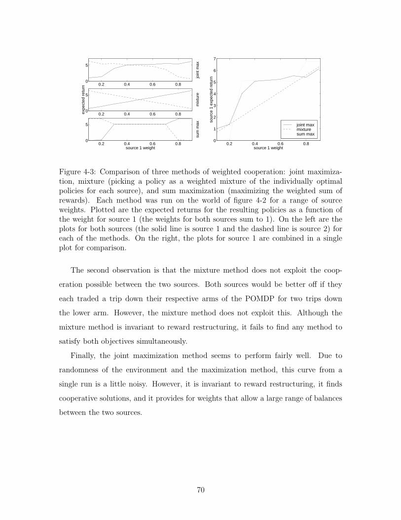
0.2 0.4 0.6 0.80
5
join
t max
0.2 0.4 0.6 0.80
5
expe
cted
ret
urn
mix
ture
0.2 0.4 0.6 0.80
5
source 1 weight
sum
max
0.2 0.4 0.6 0.80
1
2
3
4
5
6
7
source 1 weight
sour
ce 1
exp
ecte
d re
turn
joint maxmixturesum max
Figure 4-3: Comparison of three methods of weighted cooperation: joint maximiza-tion, mixture (picking a policy as a weighted mixture of the individually optimalpolicies for each source), and sum maximization (maximizing the weighted sum ofrewards). Each method was run on the world of figure 4-2 for a range of sourceweights. Plotted are the expected returns for the resulting policies as a function ofthe weight for source 1 (the weights for both sources sum to 1). On the left are theplots for both sources (the solid line is source 1 and the dashed line is source 2) foreach of the methods. On the right, the plots for source 1 are combined in a singleplot for comparison.
The second observation is that the mixture method does not exploit the coop-
eration possible between the two sources. Both sources would be better off if they
each traded a trip down their respective arms of the POMDP for two trips down
the lower arm. However, the mixture method does not exploit this. Although the
mixture method is invariant to reward restructuring, it fails to find any method to
satisfy both objectives simultaneously.
Finally, the joint maximization method seems to perform fairly well. Due to
randomness of the environment and the maximization method, this curve from a
single run is a little noisy. However, it is invariant to reward restructuring, it finds
cooperative solutions, and it provides for weights that allow a large range of balances
between the two sources.
70

4.3 Bounded Maximization
The previous section allowed for joint maximization of all objectives. We could guar-
antee that the found policy was better than a mixture of individually optimal policies.
However, sometimes we would like a different guarantee. Instead of insuring that the
policy surpasses the unknown mixture policy, we might instead wish to insure that for
some objectives, the resulting policy is better than an absolute set constant. This is a
slight relaxation of the condition that that algorithm be insensitive to reward restruc-
turing: the minimum return specified by the algorithm designer must be changed with
any reward restructuring. However, in many circumstances (like the market-marking
application of the next chapter), absolute performance measures can be set without
complete knowledge of the solution. Especially in situations where the return func-
tion is known to the designer, or where it has a well-understood interpretation, this
is a viable approach.
For the case of robot navigation towards a goal, we may wish to insure that the
robot hits obstacles with probability less than some constant. However, within the
space of policies that achieve this first objective, we want to minimize the time-to-
goal. Thus, we have two reward functions. The first penalizes for collisions and the
second rewards the robot for making it to the goal (reduced by some function of
the time the robot took). We want to find an algorithm for maximizing the second
subject to a constraint on the first.
4.3.1 Algorithm
We will designate some of the reward sources as constraint sources. For these sources,
we will associate a fixed minimum return. The optimization algorithms from previous
chapters can be modified to search only within areas of the policy space for which the
estimators’ values for the constraint sources is greater than the minimum returns.
Once again we can use a greedy search algorithm. If there is only one uncon-
strained reward source, we maximize the single source using the conjugate gradient
ascent algorithm from chapter 2. If there are multiple unconstrained reward sources,
71

we maximize them using the joint maximization algorithm in figure 4-1. To insure
that the constraints are satisfied, a few changes to the algorithms must be made.
Both algorithms use the maximization algorithm from chapter 2. This algorithm
requires a valid starting point selected from among the sampled policies. If no sampled
policy exists whose estimated returns satisfy the constraints, we discard the goal
of maximization with respect to the constraints and instead try to maximize the
constrained sources. In particular, we order the constrained sources and select the
first constrained source i for which no sampled policy conforms to all of the constraints
on sources j ≤ i. We then maximize the source i subject to the constraints on the
sources j < i. Thus, if we are concentrating on maximizing constrained source i, we
know that one of the sampled policies obeys all source constraints from 1 to i − 1.
Continuing in this manner will insure we eventually find a policy that satisfies all of
the constraints if such a policy exists. At that point we can return to optimizing the
unconstrained sources.
Additionally both algorithms search the policy space by evaluating the returns
and gradients of each source’s estimators. To insure that the algorithms stay within
the space of valid policies, we augment the return evaluation routine to return a very
small value (i.e., −∞) if any constrained source’s estimator has a value less than the
source’s constraint at the evaluation policy.
4.3.2 Results
Figure 4-4 shows a very simple abstracted robot control problem. The mobile robot
begins at point S. Its goal is to arrive in the shaded region as quickly as possible
avoiding the left wall. At each time step, it moves 1 unit of distance. It can choose
to move left, right, or down. There is a 50% chance the robot will actually move 45o
either to the left or right of the intended direction. The robot has two sources of
reward. The first rewards it for every time step during which it is in the shaded area.
The second penalizes it for every time step it runs into the left wall.
It is impossible to achieve perfect performance in this domain. No matter how
careful the robot is, if it wants to arrive at the goal position, there is some chance it
72

S
E
1 unit
soft wall (no collision penalty)
hard
wal
l (co
llisi
on p
enal
ty)
Figure 4-4: Diagram of the simulated robot collision world. The goal is for the robotto move from the start position (S) to the end position (E) without hitting the left-hand wall. At each time step, the robot has the option of moving left, right, or down.There is a 25% chance that the robot will move in a direction 45o to the left fromthe desired direction and a 25% chance it will move 45o to the right from the desireddirection on any given time step. Each time step moves the robot 1 unit of length.The robot automatically stops when it is within 1 unit of the end position. For everytime step it spends within 1 unit of the end position, it is rewarded one unit of reward.Additionally, a separate reward source rewards −1 unit of reward each time the robothits the left-hand wall. Each trial lasts for 20 time steps.
will collide with the wall. We ran the minimum reward constraint algorithm with this
world for a range of maximum allowable collisions (a maximum number of collisions
translates to a minimum reward for the collision reward source). In particular we
required the expected number of collisions to be less than values from 0.25 to 1.5
at increments of 0.25. After each run of the algorithm had converged, we measured
the true expected number of collisions and the true expected time-to-goal by running
10000 separate trails with the resulting policy. The results are shown in figure 4-
5 for a Boltzmann distribution policy class with six observation features: the cross
product of the state features (the constant 1, the x-position, and the y-position) and
two binary action features (the first is 1 only if the action is to the left and the second
is 1 only if the action is to the right).
73
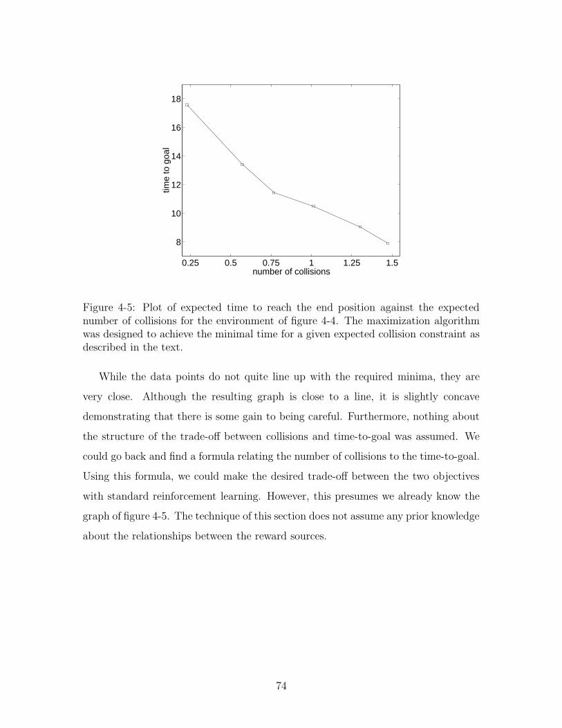
0.25 0.5 0.75 1 1.25 1.5
8
10
12
14
16
18
number of collisions
time
to g
oal
Figure 4-5: Plot of expected time to reach the end position against the expectednumber of collisions for the environment of figure 4-4. The maximization algorithmwas designed to achieve the minimal time for a given expected collision constraint asdescribed in the text.
While the data points do not quite line up with the required minima, they are
very close. Although the resulting graph is close to a line, it is slightly concave
demonstrating that there is some gain to being careful. Furthermore, nothing about
the structure of the trade-off between collisions and time-to-goal was assumed. We
could go back and find a formula relating the number of collisions to the time-to-goal.
Using this formula, we could make the desired trade-off between the two objectives
with standard reinforcement learning. However, this presumes we already know the
graph of figure 4-5. The technique of this section does not assume any prior knowledge
about the relationships between the reward sources.
74

Chapter 5
Electronic Market-Making
“Grace is given of God but knowledge is bought in the market.”
Bothie of Tober-na-Vuolich
Arthur Hugh Clough
In this chapter, we apply the algorithms developed to the problem of running a
market-making system automatically. We begin with an overview of market-making
and some of the literature to motivate the problem and our approach. We then apply
importance sampling to solve the reinforcement learning problem for two market
models. The first has theoretical bounds to which to compare our results. The second
is more complex and allows us to balance competing objectives of the market-maker.
5.1 Market-Making
Many economic markets, including most major stock exchanges, employ market-
makers to aid in the transactions and provide a better quality market. Each com-
modity has one or more market-makers assigned to it. All transactions in the market
go through a market-maker. The market-maker is responsible for setting prices and
volumes for buying and selling. If a market-maker quotes a buy price and volume
(an ask quote), this requires the market-maker to honor that price for all buy orders
75
up to the quantity indicated by the volume. The symmetric obligation holds for sell
orders (bid quotes).
Market-makers supply an advantage to the market. By consolidating the trading
in a few agents, the market becomes more efficient. Traders wishing to buy and sell do
not need to find each other or wait for each other’s arrival. Additionally, by quoting
a single price which is guaranteed for all traders, market-makers remove the price
fluctuations that occur in markets where buyers and sellers must come to their own
agreement for a price individually for each transaction. Markets with market-makers
have greater volumes and better price stability.
Market-makers themselves benefit from their position as well. They have an in-
formational advantage over regular traders because they get to see all (or many in
some cases) of the orders. The average trader does not have such information and can
only see transactions which actually take place and not all of the bids and asks that
led to the final selling price. This advantage allows market-makers to make better
predictions about the true value of a good and thereby better profits. This is regu-
lated by rules applied to market-makers and by competition in the case of multiple
market-makers. However, such an advantage is not without some risk. The market-
maker trades using his or her own personal inventory. Negative inventory puts the
market-maker at risk should the value rise and positive inventory has a similar risk
should the value drop.
5.1.1 Automating Market-Making
Many major markets are now electronic. The NASDAQ is a distributed trading
system completely run through networked computers. It uses competing market-
makers (usually one per major trading company) to maintain a high quality market.
However, the demands on human market-makers are high. A typical market-maker
will be responsible for 10 to 20 securities. At any given moment, it is only feasible
for the market-maker to be actively attentive to 2 to 3 of them. The market-maker
is generally losing potential profit or volume on the other securities.
The last few years have also seen the growth of on-line trading systems. These
76

systems are also entirely electronic and usually employ no market making. Orders
are crossed against the other orders that happen to be present at that time of the
trade and otherwise are dropped.
The goal of this chapter is to demonstrate the ability of reinforcement learning
to fill the need for automated market-making. For the case of the NASDAQ, a
learning system could fill the role of an “autopilot” by taking care of stocks in a more
intelligent manner while being supervised by a human market-maker. This would
allow a human market-maker to more successfully manage a large set of securities. In
the case of small on-line trading systems, the system could replace the existing naive
order crossing mechanism to provide a better market to its traders.
5.1.2 Previous Work
The understanding of the price formation process in security markets has been one
of the focal points of the market microstructure literature. There are two main
approaches to the market-making problem. One focuses on the uncertainties of an
order flow (the time series of orders placed) and the inventory holding risk of a market-
maker. In a typical inventory-based model, the market-maker sets the price to balance
demand and supply in the market while actively controlling its inventory holdings.
The second approach attempts to explain the price setting dynamics employing the
role of information. In information-based models, the market-maker faces traders
with superior information. The market-maker makes inferences from the orders and
sets the quotes. This informational disadvantage is reflected in the bid-ask spread
(the difference between the buy and sell prices quoted by the market-maker).
Garman (1976) describes a model in which there is a single, monopolistic, and
risk neutral market-maker who sets prices, receives all orders, and clears trades. The
dealer’s objective is to maximize expected profit per unit time. Failure of the market-
maker arises when it runs out of either inventory or cash. Arrivals of buy and sell
orders are characterized by two independent Poisson processes whose arrival rates
depend on the market-maker’s quotes. Essentially the collective activity of the traders
is modeled as a stochastic flow of orders. The solution to the problem resembles
77
that of the Gambler’s ruin problem. Garman studied several inventory-independent
strategies that lead to either a sure failure or a possible failure. The conditions to avoid
a sure failure imply a positive bid-ask spread. Garman concluded that a market-maker
must relate its inventory to the price-setting strategy in order to avoid failure. Amihud
and Mendelson (1980) extend Garman’s model by studying the role of inventory. The
problem is solved in a dynamic programming framework with inventory as the state
variable. The optimal policy is a pair of bid and ask prices, both decreasing functions
of the inventory position. The model also implies that the spread is positive, and
the market-maker has a preferred level of inventory. Ho and Stoll (1981) study the
optimal behavior of a single dealer who is faced with a stochastic demand and return
risk of his own portfolio. As in Garman (1976), orders are represented by price-
dependent stochastic processes. However, instead of maximizing expected profit, the
dealer maximizes the expected utility of terminal wealth which depends on trading
profit and returns to other components in its portfolio. Consequently the dealer’s
risks play a significant role in its price-setting strategy. One important implication of
this model is that the spread can be decomposed into two components: a risk neutral
spread that maximizes the expected profits for a set of given demand functions and a
risk premium that depends on the transaction size and return variance of the stock.
Ho and Stoll (1983) extend this to a multiple-dealer scenario. The price-dependent
stochastic order flow mechanism is common in the above studies. All preceding studies
only allow market orders traded in the market. O’Hara and Oldfield (1986) attempt
to incorporate more realistic features of real markets into their analysis. Their paper
studies a dynamic pricing policy of a risk-averse market-maker who receives both limit
and market orders and faces uncertainty in the inventory valuation. The optimal
pricing strategy takes into account the nature of the limit and market orders as well
as inventory risk.
Inventory-based models focus on the role of order flow uncertainty and inventory
risk in the determination of the bid-ask spread. The information-based approach
suggests that the bid-ask spread could be a purely informational phenomenon irre-
spective of inventory risk. Glosten and Milgrom (1985) study the market-making
78
problem in a market with asymmetric information. In the Glosten-Milgrom model
some traders have superior (insider) information and others do not. Traders consider
their information and submit orders to the market sequentially. The market-maker,
which does not have any information advantage, sets its prices, conditioning on all
the available information such that the expected profit on any trade is zero. Specif-
ically, the specialist sets its prices equaled the conditional expectation of the stock
value given past transactions. Its main finding is that in the presence of insiders, a
positive bid-ask spread would exist even when the market-maker is risk-neutral and
make zero expected profit.
Most of these studies have developed conditions for optimality but provided no
explicit price adjustment policies. For example, in Amihud and Mendelson (1980),
bid and ask prices are shown to relate to inventory but the exact dependence is
unavailable. Some analyses do provide functional forms of the bid/ask prices (such as
O’Hara and Oldfield (1986)) but the practical applications of the results are limited
due to stringent assumptions made in the models.
The reinforcement learning models developed in this chapter make few assump-
tions about the market environment and yield explicit price setting strategies. We
will start with a simple model where theoretical analysis is possible and then move
to a more complex model with multiple objectives.
5.2 Simple Model
Our goal for this section is to develop a simple model that adequately simulates the
strategy of a trading crowd given the quotes of a market-maker. Information-based
models focusing on information asymmetry provide the basis for our basic model. In
a typical information-based model, there is a group of informed traders or insiders
who have superior information about the true value of the stock and a group of
uninformed traders who possess only public information. The insiders buy whenever
the market-maker’s prices are too low and sell whenever they are too high based on
their private information; the uninformed simply trade randomly for liquidity needs.
79

A single market-maker is at the center of trading in the market. It posts the bid and
ask prices at which all trades transact. Due to the informational disadvantage, the
market-maker always loses to the insiders while breaking even with the uninformed.
5.2.1 Model Description
To further illustrate this idea of asymmetric information among different traders,
consider the following case. A single security is traded in the market. There are
three types of participants: a monopolistic market-maker, insiders, and uninformed
traders. The market-maker sets one price at which the next arriving trader has the
option to either buy or sell one share. In other words, it is assumed that the bid price
equals the ask price. Traders trade only with market orders. All orders are executed
by the market-maker and there are no crossings of orders among traders. After the
execution of an order, the market-maker can adjust its quotes given its knowledge of
past transactions.
To further simplify the problem, we allow the market-maker to have negative
inventory and cash. We assume the resources of the company running the market-
making are vast enough to allow this. Furthermore, the position is liquidated at the
end of the day, limiting the risk of such a method. For real markets, the details
of the market’s closing are complex and individual to the particular market. How-
ever, because the securities can shift and change overnight, it is common practice
for market-makers to return their inventory to zero at the close of the market. The
closing mechanism for many markets also serves to converge on a single price for each
security. This means that calculating the profit at the end of the day is reasonable
and in many cases part of the normal closing function of the market. For simplicity,
events in the market occur at discrete time steps. In particular, events are modeled
as independent Poisson processes. These events include the change of the security’s
true price and the arrival of informed and uninformed orders.
There exists a true price p∗ for the security. The idea is that there is an exogenous
process that completely determines the value of the stock. The true price is to be
distinguished from the market price which is determined by the interaction between
80

the market-maker and the traders. The price p∗ follows a Poisson jump process. In
particular, it makes discrete jumps, upward or downward with a probability λp at
each time step. The size of the discrete jump is a constant 1. The true price, p∗, is
given to the insiders but not known to the uninformed traders or the market-maker.
The insider and uninformed traders arrive at the market with a probability of
λi and 2λu respectively.1 Insiders are the only ones who observe the true price of
the security. They can be considered as investors who acquire superior information
through research and analysis. They compare the true price with market-maker’s
price and will buy (sell) one share if the true price is lower (higher) than the market-
maker’s price, and will submit no orders otherwise. Uninformed traders will place
orders to buy and sell a security randomly. The uninformed merely re-adjust their
portfolios to meet liquidity needs, which is not modeled in the market. Hence they
simply submit buy or sell orders of one share randomly with equal probabilities λu.
All independent Poisson processes are combined together to form a new Poisson
process. Furthermore, it is assumed that there is one arrival of an event at each time
step. Hence, at any particular time step, the probability of a change in the true price
is 2λp, that of an arrival of an insider is λi, and that of an arrival of an uninformed
trader is 2λu. Since there is a guaranteed arrival of an event, all probabilities sum up
to one: 2λp + 2λu + λi = 1.
Each trial of the market represents one trading day. The market begins with the
true price and the market-maker’s price both set to the arbitrary value of 100. At
every time step the market-maker observes whether a buy, a sell, or neither took
place and has the chance to increase or decrease its price by 1 unit. At the end of
the trading day (100 time steps), the inventory is liquidated at the current true price
resulting in the profit (or loss) of the market-maker.
The uninformed traders represent noise in the market. By randomly trading, they
obscure the information available from the informed traders’ trades. The market-
maker cannot differentiate between orders placed by informed traders and those
placed by uninformed traders. For the results in this chapter, we use the term noise
1Buy and sell orders from the uninformed traders each arrive at a probability of λu.
81
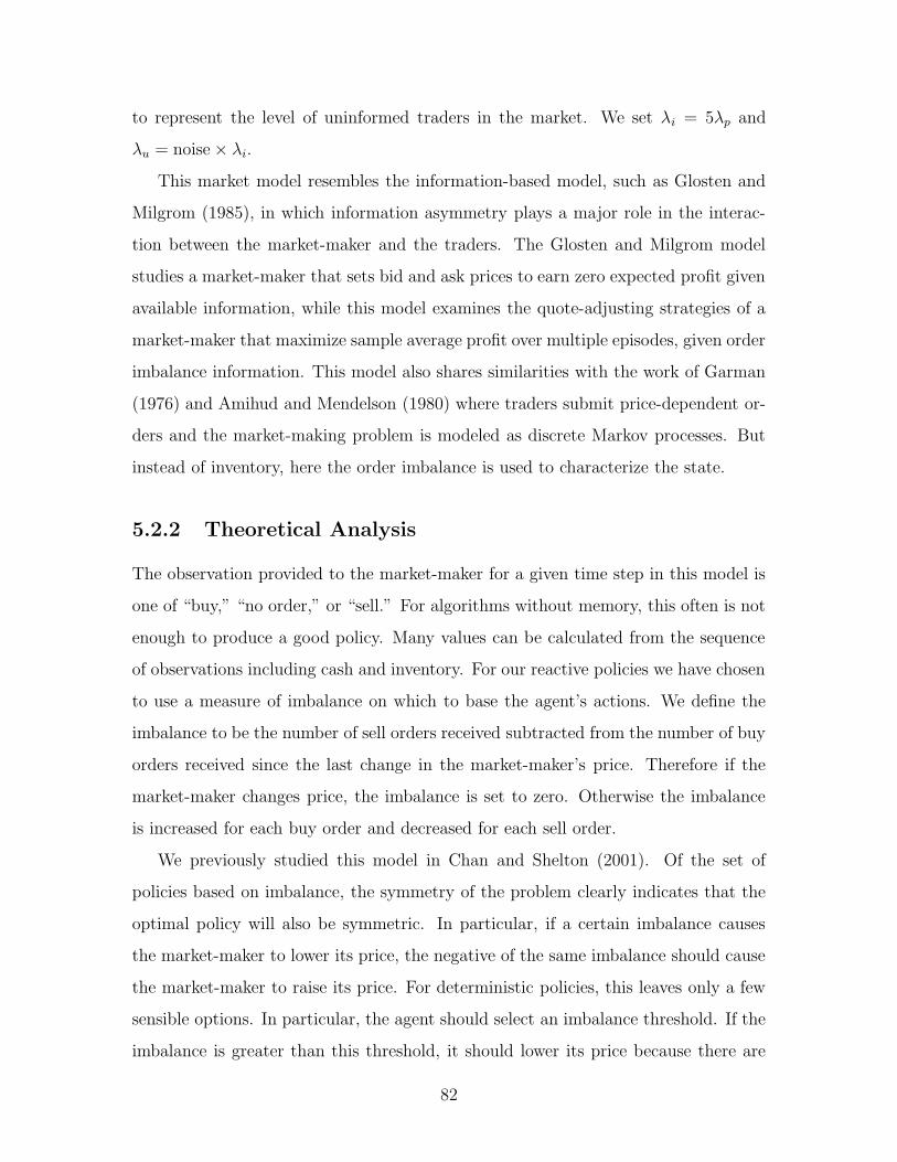
to represent the level of uninformed traders in the market. We set λi = 5λp and
λu = noise× λi.
This market model resembles the information-based model, such as Glosten and
Milgrom (1985), in which information asymmetry plays a major role in the interac-
tion between the market-maker and the traders. The Glosten and Milgrom model
studies a market-maker that sets bid and ask prices to earn zero expected profit given
available information, while this model examines the quote-adjusting strategies of a
market-maker that maximize sample average profit over multiple episodes, given order
imbalance information. This model also shares similarities with the work of Garman
(1976) and Amihud and Mendelson (1980) where traders submit price-dependent or-
ders and the market-making problem is modeled as discrete Markov processes. But
instead of inventory, here the order imbalance is used to characterize the state.
5.2.2 Theoretical Analysis
The observation provided to the market-maker for a given time step in this model is
one of “buy,” “no order,” or “sell.” For algorithms without memory, this often is not
enough to produce a good policy. Many values can be calculated from the sequence
of observations including cash and inventory. For our reactive policies we have chosen
to use a measure of imbalance on which to base the agent’s actions. We define the
imbalance to be the number of sell orders received subtracted from the number of buy
orders received since the last change in the market-maker’s price. Therefore if the
market-maker changes price, the imbalance is set to zero. Otherwise the imbalance
is increased for each buy order and decreased for each sell order.
We previously studied this model in Chan and Shelton (2001). Of the set of
policies based on imbalance, the symmetry of the problem clearly indicates that the
optimal policy will also be symmetric. In particular, if a certain imbalance causes
the market-maker to lower its price, the negative of the same imbalance should cause
the market-maker to raise its price. For deterministic policies, this leaves only a few
sensible options. In particular, the agent should select an imbalance threshold. If the
imbalance is greater than this threshold, it should lower its price because there are
82
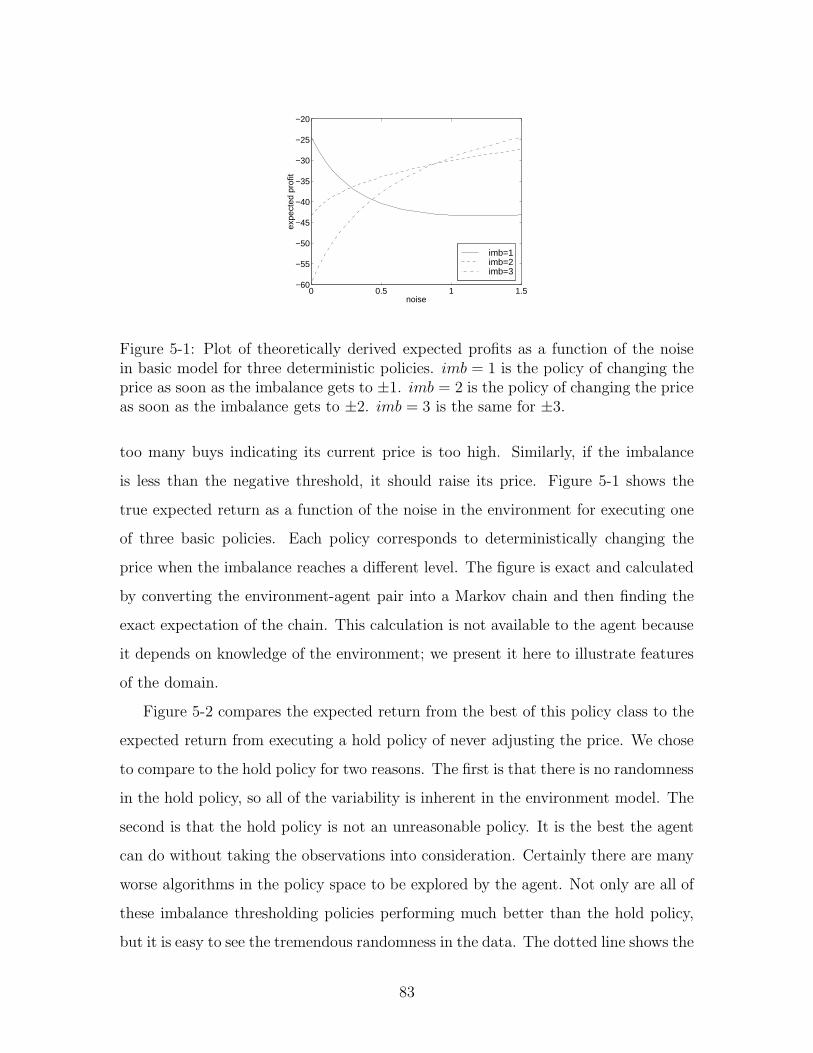
0 0.5 1 1.5−60
−55
−50
−45
−40
−35
−30
−25
−20
noiseex
pect
ed p
rofit
imb=1imb=2imb=3
Figure 5-1: Plot of theoretically derived expected profits as a function of the noisein basic model for three deterministic policies. imb = 1 is the policy of changing theprice as soon as the imbalance gets to ±1. imb = 2 is the policy of changing the priceas soon as the imbalance gets to ±2. imb = 3 is the same for ±3.
too many buys indicating its current price is too high. Similarly, if the imbalance
is less than the negative threshold, it should raise its price. Figure 5-1 shows the
true expected return as a function of the noise in the environment for executing one
of three basic policies. Each policy corresponds to deterministically changing the
price when the imbalance reaches a different level. The figure is exact and calculated
by converting the environment-agent pair into a Markov chain and then finding the
exact expectation of the chain. This calculation is not available to the agent because
it depends on knowledge of the environment; we present it here to illustrate features
of the domain.
Figure 5-2 compares the expected return from the best of this policy class to the
expected return from executing a hold policy of never adjusting the price. We chose
to compare to the hold policy for two reasons. The first is that there is no randomness
in the hold policy, so all of the variability is inherent in the environment model. The
second is that the hold policy is not an unreasonable policy. It is the best the agent
can do without taking the observations into consideration. Certainly there are many
worse algorithms in the policy space to be explored by the agent. Not only are all of
these imbalance thresholding policies performing much better than the hold policy,
but it is easy to see the tremendous randomness in the data. The dotted line shows the
83
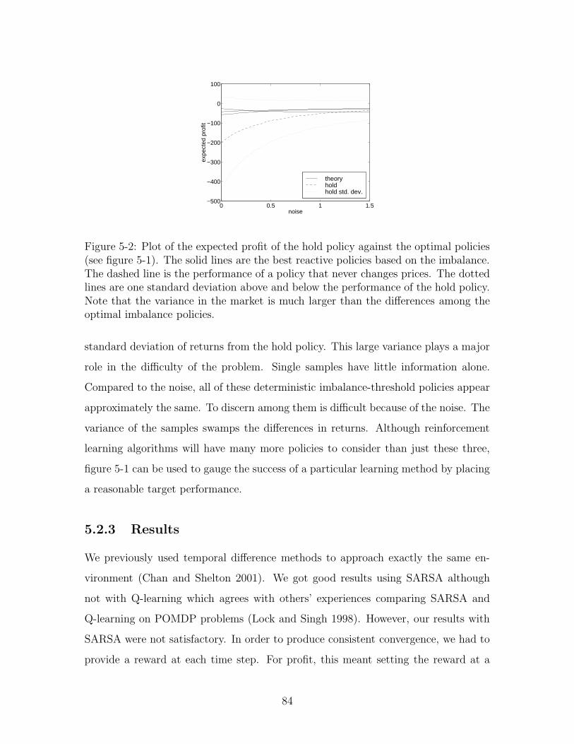
0 0.5 1 1.5−500
−400
−300
−200
−100
0
100
noiseex
pect
ed p
rofit
theoryholdhold std. dev.
Figure 5-2: Plot of the expected profit of the hold policy against the optimal policies(see figure 5-1). The solid lines are the best reactive policies based on the imbalance.The dashed line is the performance of a policy that never changes prices. The dottedlines are one standard deviation above and below the performance of the hold policy.Note that the variance in the market is much larger than the differences among theoptimal imbalance policies.
standard deviation of returns from the hold policy. This large variance plays a major
role in the difficulty of the problem. Single samples have little information alone.
Compared to the noise, all of these deterministic imbalance-threshold policies appear
approximately the same. To discern among them is difficult because of the noise. The
variance of the samples swamps the differences in returns. Although reinforcement
learning algorithms will have many more policies to consider than just these three,
figure 5-1 can be used to gauge the success of a particular learning method by placing
a reasonable target performance.
5.2.3 Results
We previously used temporal difference methods to approach exactly the same en-
vironment (Chan and Shelton 2001). We got good results using SARSA although
not with Q-learning which agrees with others’ experiences comparing SARSA and
Q-learning on POMDP problems (Lock and Singh 1998). However, our results with
SARSA were not satisfactory. In order to produce consistent convergence, we had to
provide a reward at each time step. For profit, this meant setting the reward at a
84
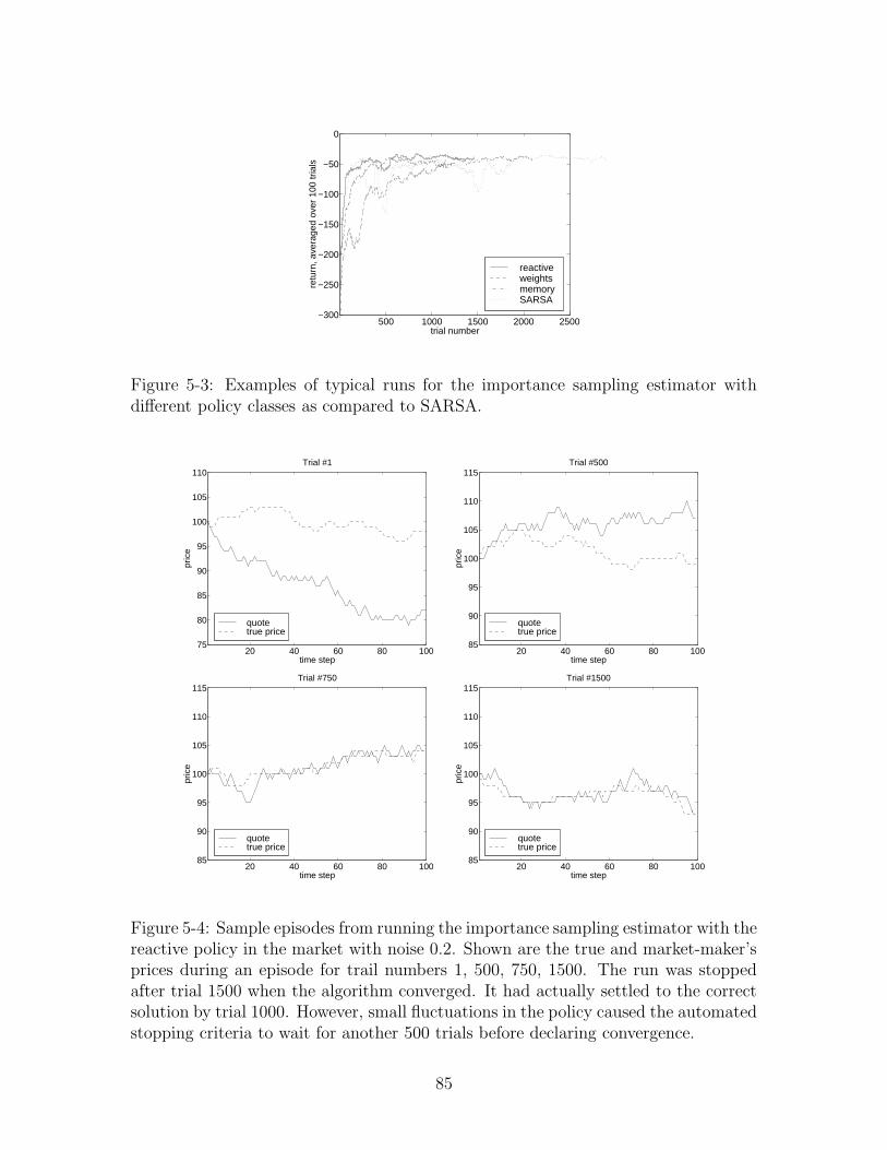
500 1000 1500 2000 2500−300
−250
−200
−150
−100
−50
0
trial number
retu
rn, a
vera
ged
over
100
tria
ls
reactiveweightsmemorySARSA
Figure 5-3: Examples of typical runs for the importance sampling estimator withdifferent policy classes as compared to SARSA.
20 40 60 80 10075
80
85
90
95
100
105
110
time step
pric
e
Trial #1
quotetrue price
20 40 60 80 10085
90
95
100
105
110
115
time step
pric
eTrial #500
quotetrue price
20 40 60 80 10085
90
95
100
105
110
115
time step
pric
e
Trial #750
quotetrue price
20 40 60 80 10085
90
95
100
105
110
115
time step
pric
e
Trial #1500
quotetrue price
Figure 5-4: Sample episodes from running the importance sampling estimator with thereactive policy in the market with noise 0.2. Shown are the true and market-maker’sprices during an episode for trail numbers 1, 500, 750, 1500. The run was stoppedafter trial 1500 when the algorithm converged. It had actually settled to the correctsolution by trial 1000. However, small fluctuations in the policy caused the automatedstopping criteria to wait for another 500 trials before declaring convergence.
85
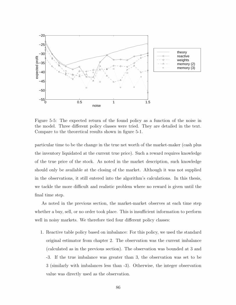
0 0.5 1 1.5−55
−50
−45
−40
−35
−30
−25
−20
noise
expe
cted
pro
fit
theoryreactiveweightsmemory (2)memory (3)
Figure 5-5: The expected return of the found policy as a function of the noise inthe model. Three different policy classes were tried. They are detailed in the text.Compare to the theoretical results shown in figure 5-1.
particular time to be the change in the true net worth of the market-maker (cash plus
the inventory liquidated at the current true price). Such a reward requires knowledge
of the true price of the stock. As noted in the market description, such knowledge
should only be available at the closing of the market. Although it was not supplied
in the observations, it still entered into the algorithm’s calculations. In this thesis,
we tackle the more difficult and realistic problem where no reward is given until the
final time step.
As noted in the previous section, the market-market observes at each time step
whether a buy, sell, or no order took place. This is insufficient information to perform
well in noisy markets. We therefore tied four different policy classes:
1. Reactive table policy based on imbalance: For this policy, we used the standard
original estimator from chapter 2. The observation was the current imbalance
(calculated as in the previous section). The observation was bounded at 3 and
-3. If the true imbalance was greater than 3, the observation was set to be
3 (similarly with imbalances less than -3). Otherwise, the integer observation
value was directly used as the observation.
86
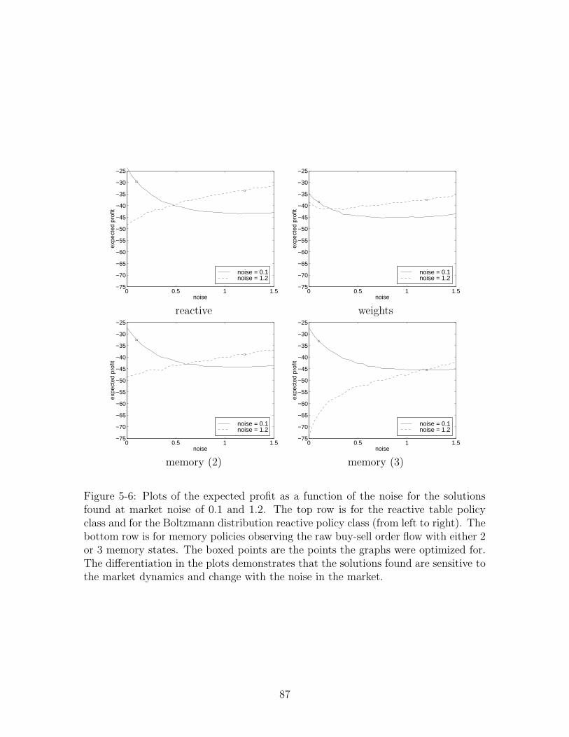
0 0.5 1 1.5−75
−70
−65
−60
−55
−50
−45
−40
−35
−30
−25
noise
expe
cted
pro
fit
noise = 0.1noise = 1.2
0 0.5 1 1.5−75
−70
−65
−60
−55
−50
−45
−40
−35
−30
−25
noiseex
pect
ed p
rofit
noise = 0.1noise = 1.2
reactive weights
0 0.5 1 1.5−75
−70
−65
−60
−55
−50
−45
−40
−35
−30
−25
noise
expe
cted
pro
fit
noise = 0.1noise = 1.2
0 0.5 1 1.5−75
−70
−65
−60
−55
−50
−45
−40
−35
−30
−25
noise
expe
cted
pro
fit
noise = 0.1noise = 1.2
memory (2) memory (3)
Figure 5-6: Plots of the expected profit as a function of the noise for the solutionsfound at market noise of 0.1 and 1.2. The top row is for the reactive table policyclass and for the Boltzmann distribution reactive policy class (from left to right). Thebottom row is for memory policies observing the raw buy-sell order flow with either 2or 3 memory states. The boxed points are the points the graphs were optimized for.The differentiation in the plots demonstrates that the solutions found are sensitive tothe market dynamics and change with the noise in the market.
87
2. Policy weights based on Boltzmann distribution using imbalance: For this pol-
icy, we used the Boltzmann distribution for a policy class with weights as in
section 3.2. The observation feature vector had four features. The first two
were 1 and the imbalance if the action was to lower the price. Otherwise, they
were both 0. The second two were 1 and the imbalance if the action was to
raise the price (and otherwise 0).
3. Memory policy with 2 memory states based on the raw observations: For this
policy, the imbalance was not computed automatically for the agent. Instead,
it was given two memory states (as in section 3.1) and the raw observations of
buy, sell, or no action.
4. Memory policy with 3 memory states based on the raw observations: as above,
but with three memory states.
We let θ (from section 3.3) be 0.03 for all experiments in this chapter to combat the
noise inherent in the problem. The experiments were run until on twenty consecutive
trials, no policy parameter changed by more than 0.01 and the estimated return for
the policy changed by no more than 0.1. We ran each of these four policy classes on
the market model, varying the noise from 0.0 to 1.5 at increments of 0.1.
Figure 5-3 compares a sample run of each algorithm and SARSA (using the reac-
tive table policy class based on imbalance) for a market with noise of 0.2. We can see
that the SARSA method takes longer to converge and can become unstable later. It
often will jump to strange policies after seeming convergence. Faster annealing of the
SARSA learning rate causes the algorithm to fail to converge. Although not as appar-
ent due to the smoothing, the SARSA algorithm produced some very negative returns
for a couple of trials in a row and then returned to its previous performance (this
can be seen by the dips in the graph at about 500 and 1500 trials). By comparison,
the importance sampling estimators behave more nicely in this partially observable
environment.
To show the adaptation of the learning algorithm, figure 5-4 shows the price
dynamics for three episodes during one run of the algorithm. We can see that as the
88
agent gathers more experience, it is better able to track the true price of the stock.
Figure 5-5 shows the expected returns (measured by 10000 separate trials taken
after learning had converged) for each algorithm as a function of the noise. We notice
that the two policies based on imbalance come close to meeting the theoretical bounds
of the solid line. The two policies based on memory fair more poorly. However, it
should be noted that, as shown in figure 5-2, all of these policies perform very well
compared to holding even and the noise inherent in the model.
To demonstrate that the learned policies are sensitive to the particulars of the
market environment (in this case, the noise), figure 5-6 compares the policies found
at noise 0.1 to those found at 1.2. We took the policies found for both noise settings
and plotted how those policies would perform across all noise levels. We can see that
for each policy class, the algorithm finds a different type of solution and that the
solutions found for noise 0.1 are different than those at 1.2.
5.3 Spread Model
The previous section demonstrates how reinforcement learning algorithms can be ap-
plied to market-making problems and successfully converge to competitive strategies
under different circumstances. Although the basic model is useful because the exper-
imental and theoretical results can be compared, one of its major limitations is the
equality of the bid and ask prices. Without the bid-ask spread the market-maker suf-
fers a loss from the market due to the information disadvantage. A natural extension
of the basic model is to let the market-maker quote bid and ask prices. The rest of
the market remains the same. Informed traders sell if the bid price is too high and
buy if the ask is too low. Uninformed traders still trade randomly. Each transaction
is for the fixed volume of 1 share.
The market-maker now has two objectives. It wants to maximize profits to insure a
stable business platform. It also wants to minimize the average spread. By minimizing
spread, the market-maker insures better volume (more trades through the market-
making system) because it provides more competitive prices. Because of the increased
89

volume, the company running the market-maker can provide better deals to its private
investors.
5.3.1 Model Description
To incorporate bid and ask prices to the model, the set of actions is augmented to
include the change of the bid price and the change of the ask price. Thus the agent
has 9 action choices corresponding to each possible pair of actions with respect to
the bid and ask prices (each can be raised, kept the same, or lowered). The spread
also enters the reward function to regulate the of market quality maintained by the
agent. The profit and spread rewards are separate sources. The profit source is as in
the previous model. The spread source’s reward at a time step is the negative spread.
Thus the return from this source is the negative sum of the spread over all time steps.
In the basic model, the market-maker only aims at maximizing profit. By adding
spread to the model, the market-maker also needs to consider the quality of market
it provides. If it only seeks to maximize profits, it can create a huge spread and
gain profit from the uninformed traders. Unfortunately, this results in low market
quality and a loss in volume (as mentioned above). These objectives are not entirely
competitive: some policies result in poor profits and large spreads. However, for the
most part, increases in profit come at the expense of reduced spreads. The exact
trade-off is a function of the market and unknown.
5.3.2 Results
The most natural method to balance the rewards is to fix a desired minimum expected
profit find the minimal average spread policy subject to the profit constraint. Such
a constraint may be set by the operators of the market-maker to insure reasonable
profitability. For these experiments, we used the bounded maximization method from
section 4.3 to achieve this goal. The average profit per day was fixed between −15 and
15 and the negative average spread (the second reward source) was maximized. The
results from the previous section were assumed. The default policy therefore lowers
90
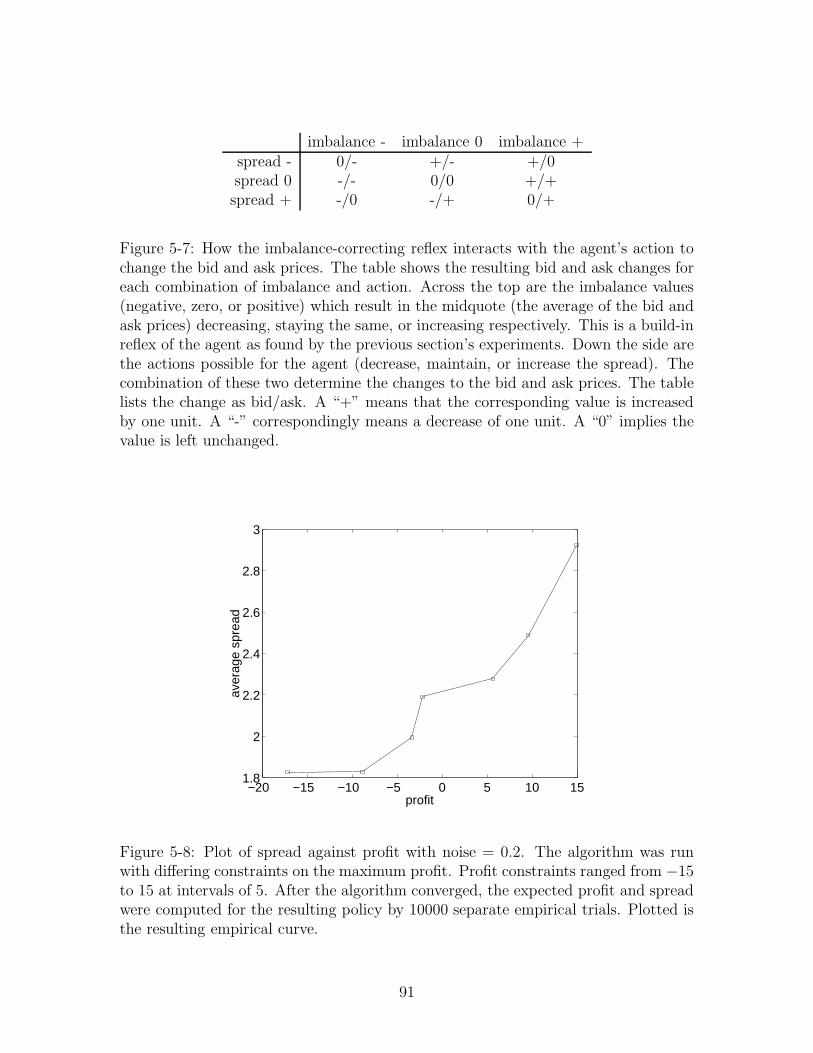
imbalance - imbalance 0 imbalance +spread - 0/- +/- +/0spread 0 -/- 0/0 +/+spread + -/0 -/+ 0/+
Figure 5-7: How the imbalance-correcting reflex interacts with the agent’s action tochange the bid and ask prices. The table shows the resulting bid and ask changes foreach combination of imbalance and action. Across the top are the imbalance values(negative, zero, or positive) which result in the midquote (the average of the bid andask prices) decreasing, staying the same, or increasing respectively. This is a build-inreflex of the agent as found by the previous section’s experiments. Down the side arethe actions possible for the agent (decrease, maintain, or increase the spread). Thecombination of these two determine the changes to the bid and ask prices. The tablelists the change as bid/ask. A “+” means that the corresponding value is increasedby one unit. A “-” correspondingly means a decrease of one unit. A “0” implies thevalue is left unchanged.
−20 −15 −10 −5 0 5 10 151.8
2
2.2
2.4
2.6
2.8
3
profit
aver
age
spre
ad
Figure 5-8: Plot of spread against profit with noise = 0.2. The algorithm was runwith differing constraints on the maximum profit. Profit constraints ranged from −15to 15 at intervals of 5. After the algorithm converged, the expected profit and spreadwere computed for the resulting policy by 10000 separate empirical trials. Plotted isthe resulting empirical curve.
91
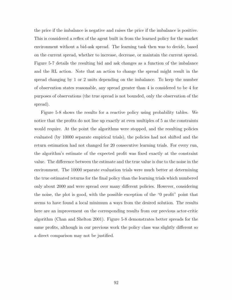
the price if the imbalance is negative and raises the price if the imbalance is positive.
This is considered a reflex of the agent built in from the learned policy for the market
environment without a bid-ask spread. The learning task then was to decide, based
on the current spread, whether to increase, decrease, or maintain the current spread.
Figure 5-7 details the resulting bid and ask changes as a function of the imbalance
and the RL action. Note that an action to change the spread might result in the
spread changing by 1 or 2 units depending on the imbalance. To keep the number
of observation states reasonable, any spread greater than 4 is considered to be 4 for
purposes of observations (the true spread is not bounded, only the observation of the
spread).
Figure 5-8 shows the results for a reactive policy using probability tables. We
notice that the profits do not line up exactly at even multiples of 5 as the constraints
would require. At the point the algorithms were stopped, and the resulting policies
evaluated (by 10000 separate empirical trials), the policies had not shifted and the
return estimation had not changed for 20 consecutive learning trials. For every run,
the algorithm’s estimate of the expected profit was fixed exactly at the constraint
value. The difference between the estimate and the true value is due to the noise in the
environment. The 10000 separate evaluation trials were much better at determining
the true estimated returns for the final policy than the learning trials which numbered
only about 2000 and were spread over many different policies. However, considering
the noise, the plot is good, with the possible exception of the “0 profit” point that
seems to have found a local minimum a ways from the desired solution. The results
here are an improvement on the corresponding results from our previous actor-critic
algorithm (Chan and Shelton 2001). Figure 5-8 demonstrates better spreads for the
same profits, although in our previous work the policy class was slightly different so
a direct comparison may not be justified.
92
5.4 Discussion
We feel these results clearly demonstrate the power of our importance sampling algo-
rithm. The models of this chapter are highly stochastic and provide difficult challenges
for reinforcement learning algorithms. We were able to show that our algorithm is
can find good solutions in the presence of large amounts of noise while at the same
time remaining sensitive to small differences in the market. Furthermore, we were
able to successfully balance two major objectives of real market-makers in a simple
framework that allows for a natural specification of the desired trade-off between the
objectives.
93

94
Chapter 6
Conclusions
“Error has no end.”
Paracelsus. Part iii.
Robert Browning
We feel this thesis represents the first major exploration of importance sampling
for reinforcement learning. There have been only two previous uses of importance
sample in RL. The first (Precup, Sutton, and Singh 2000; Precup, Sutton, and Das-
gupta 2001) used importance sampling as a slight modification to temporal differ-
ence learning. The second (Peshkin and Mukherjee 2001) developed some theoretical
bounds for importance sampling, but did not develop any algorithms or experimental
results.
We have extended importance sampling to multiple sampling policies, demon-
strated it can be calculated for not only reactive table-based policies, but also param-
eterized policies and finite-state controllers. We have given exact variance formulae
for the estimates. Furthermore, we have demonstrated the power of the full return
surface estimate provided by our importance sampling method in solving problems
with multiple objectives. Finally, we have demonstrated its success on numerous
small problems and ultimately on the practical and highly noisy domain of electronic
market-making.
95
Electronic market-making is a real problem with few robust automatic techniques.
Reinforcement learning shows promise of making useful progress on this practical and
important domain. However, as this is the first serious use of importance sampling
and only the second attempt to apply reinforcement learning to market-making, there
are a number of immediate and future problems to be tackled. We feel that all of
them are possible given the foundations laid in this thesis.
6.1 Algorithm Components
The algorithm of this thesis is composed of a number of components. Each could
individually benefit from some additional research.
6.1.1 Estimator Performance
We think the normalized estimator works very well given the minimal assumptions
made. These assumptions allow the algorithm to work in almost any reinforcement
learning scenario, yet we still take into consideration the temporal control problem
inherent to reinforcement learning. The time series of observations, action, and re-
wards are explicit in calculating the importance sampling ratios. When combined
with a greedy algorithm, the estimator produces quick learning.
Yet, we feel that two immediate extensions might help. The first is to provide
error estimates or bounds on the return estimate. We have a formula for the variance
of the estimator, but we still need a good estimate of this variance from the samples
(direct application of the formula requires full knowledge of the POMDP). Although
we provide a simple variance estimate of sorts in section 3.3, it is not theoretically
rigorous.
Second, the estimate needs to be “sparsified.” After n trials, computing the
estimate (or its derivative) for a given policy takes O(n) work. This makes the
entire algorithm quadratic in the number of trials. However, a similar estimate could
probably be achieved with fewer points. Remembering only the important trials
would produce a simpler estimate.
96
More generally, improved insight and theory may come from more study of the
basic research in importance sampling. Yet, it is difficult to bring the results from
importance sampling to this problem. Importance sampling usually assumes that the
designer has control over the sampling distribution. In our problem, we’d like to allow
the agent to use experience that was sampled in any fashion. Whereas importance
sampling often asks, “given an expectation to estimate, how should I sample to reduce
the variance of the estimate?” we would like to ask “given a sampling method, how
best should I estimate the expectation to reduce variance?” Hesterberg (1995) does
list a number of other importance sampling methods. Unfortunately none of them
are computable in this case (recall that the full probability function is not available,
only one factor of it).
Finally, it may seem disturbing that we must remember which policies were used
on each trial. The return doesn’t really depend on the policy that the agent wants
to execute; it only depends on how the agent actually does act. In theory we should
be able to forget which policies were tried; doing so would allow us to use data which
was not gathered with a specified policy. The policies are necessary in this paper as
proxies for the unobserved state sequences. We hope future work might be able to
remove this dependence.
6.1.2 Greedy Search
The greedy search algorithms used are simple and can be effective for environments
with little noise and where the optimal policies are near the boundaries of the policy
space. However, not all problems exhibit these properties. Although the variance-
controlled search algorithm of section 3.3 does help, it is not a complete solution.
The greedy search is prone to getting stuck in local minimum and in general, the
variance-control does not help in this respect. The most obvious example of local
minima is in the simple problem of maximizing the estimated return function. This
problem is unsurmountable in general and will only be improved with better general
function maximization algorithms.
However, the more addressable and less fundamental difficulty is in picking ex-
97

ploration policies. Although, given enough samples, the estimate will eventually
converge to the true return, if those samples are drawn from policies far from the
optimal distribution, it may take a long time before convergence. In fact, it may take
long enough that the algorithm appears to have converged to a suboptimal procedure
even though the function maximization algorithm is not stuck in local minima. The
problem is not that the maximization procedure could not find the global maximum
of the return surface, but rather that the global maximum of the estimated return is
actually only a local maximum of the true return.
The algorithm needs to select sampling policies for the potential information they
will supply to the estimator in addition to the potential immediate return. Whether
such a choice requires more assumptions about the environment is unclear. However,
a more clever sampling procedure would certainly lead to faster convergence with
fewer local minima problems.
6.1.3 Multiple Objectives
We do not feel that multiple objectives have been given enough attention in the RL
literature. They are crucial to the application of RL to many real-world applications.
It is often nearly impossible for a designer of a system to sit down and write out an
exact expression for a single reward function that will lead to the desired behavior.
More often it is only practical for the designer to create separate reward functions for
each sub-behavior or sub-goal of the agent.
These sub-goals usually interact in one of a number of different ways first presented
by Kaelbling (2001):
1. Conjunctive: The agent must achieve all goals.
2. Consecutive: The agent must perform each task in serial.
3. Simultaneous: The agent must maintain all goals at the same time.
4. Conditional: The agent must perform one goal while maintaining a minimum
level of performance on another goal.
98
The first interaction form is difficult to define more carefully without specifying a sin-
gle reward function that captures the way in which trade-offs among the goals should
be balanced should they not all be maximally obtainable simultaneously. Without
additional knowledge, it may not be practical to address this interaction style. The
second form is well covered by standard reinforcement learning methods. Each policy
is learned individually and executed in series. It makes the implicit assumption that
achieving one goal does not undo the gains from achieving other goals.
The last two forms are addressed by this thesis. The simultaneous objectives
are covered by the joint maximization algorithm of chapter 4 and the conditional
objectives are covered by the conditional maximization algorithm of the same chapter.
These two forms are particularly crucial for designing systems by multiple reward
source specifications. The entire purpose for specifying multiple reward sources is
that the exact method of combination is unknown. Both of the algorithms in this
thesis have tunable parameters that have natural interpretations which regards to
balancing the rewards, and yet do not require a priori knowledge about the optimal
policy. In this way, the reward designer can create sub-goals and reason about the
correct parameter settings to balance the objectives. Furthermore, the parameters can
be adjusted easily if the resulting behavior does not match the designer’s expectations.
We think that there is more to be done however. In particular, for the simultaneous
objectives, a better overall objective needs to formulated so that different algorithms
can be compared. Additionally, it would be nice if complex single reward sources could
be automatically broken down into multiple sources. The additional complexity of
the multiple sources may be overcome by the ease of learning with simpler reward
function.
6.2 Market-Making
Not only are we excited about the possibilities of importance sampling for reinforce-
ment learning, we are excited about the possibilities of reinforcement learning for
market-marking. This domain is growing with the increasing number of markets
99

moving to electronic domains. Not only is this a practical and useful problem to
solve with many of the complications of real-world domains, it is an environment
well-suited to electronic and algorithmic control. The market structure is mathemat-
ical, events occur at distinct points in time, and the entire environment is electronic
making the interface simple. Market-making differs from general portfolio manage-
ment in that market-makers have a legitimate information advantage allowing them
to make a profit even in a rational market. The potential for useful algorithms is very
high.
We also see great potential from the scalability of market-making. Additional
information and model complexity can be added gradually much as we did in this
thesis by first solving the basic market model and then using the results from that as
reflexes for the policies of the spread model. We hope that this technique can con-
tinue, allowing the addition of more complex environment models involving additional
information sources including financial news and related markets.
It would seem that any system employed in a real market will require adaptive fea-
tures to allow it to adjust to market changes. Reinforcement learning and importance
sampling in particular shows the promise of providing such adaptive systems.
100
Appendix A
Bias and Variance Derivations
We will assume that the policy we are evaluating is πA and thus we are interested
in estimating E[R|πA]. Later, we will look at the difference between the estimate at
point πA and at point πB. All sums are over the data points (1 through n) unless
otherwise noted. Integrals will be over the space of histories. If the space of histories
is discrete (as is the case for POMDPs), these should actually be sums. However, by
using integrals for histories and sums for experience, the notation becomes clearer.
To aid in the derivation of the bias and variance of the estimators, we will define
a few symbols to represent common quantities and simplify the notation.
p(h)4=
1
n
∑
i
p(h|πi)
p(h, g)4=
1
n
∑
i
p(h|πi)p(g|πi) .
These are mixture distributions that represent the average sampling distribution.
wiA
4=
p(hi|πA)
p(hi)
wiB
4=
p(hi|πB)
p(hi).
These are the unnormalized sample weights for the estimates at πA and πB respec-
101
tively.
Ri 4= R(hi)
riA
4= Riwi
A
riB
4= Riwi
B
RA4= E[R|πA]
RB4= E[R|πB] .
Finally, these are the sampled returns, the weighted returns, and the true expectation
values.
A.1 Unnormalized Estimator
First we consider the unnormalized estimator
U(πA) =1
n
∑
i
riA .
Its mean can easily be derived as
E[U(πA)] = E[1
n
∑
i
riA]
=1
n
∑
i
E[riA]
=1
n
∑
i
∫
R(hi)p(hi|πA)
p(hi)p(hi|πi) dhi
=1
n
∑
i
∫
R(h)p(h|πA)
p(h)p(h|πi) dh
=
∫
R(h)p(h|πA)
p(h)
1
n
∑
i
p(h|πi) dh
=
∫
R(h)p(h|πA)
p(h)p(h) dh
=
∫
R(h)p(h|πA) dh
102

= E[R|πA]
= RA
and thus U(πA) is an unbiased estimate of RA. Similarly, we can derive that
1
n
∑
i
E[riB] = RB
1
n
∑
i
E[wiA] = 1
1
n
∑
i
E[wiB] = 1
which will be useful later.
We can also find the variance of this estimator:
E [(U(πA) − E[U(πA)])2]
= E[(1
n
∑
i
riA)2]−R2
A
=1
n2
∑
i
E[(riA)2] +
1
n2(∑
i
E[riA])2 −
1
n2
∑
i
E[riA]2 − R2
A
=1
n
(
1
n
∑
i
E[(riA)2]−
1
n
∑
i
E[riA]2
)
=1
n
(∫
R2(h)p(h|πA)
p(h)p(h|πA) dh−
∫∫
R(h)R(g)p(h, g)
p(h)p(g)p(h|πA)p(g|πA) dh dg
)
.
Although this might look a bit messy, there is sense in it. The quantity inside the
parentheses is constant if, as n increases, the chosen policies (πi) remain the same.
This would happen if we kept the same set of trial policies and just kept cycling
through them. In fact, if all of the πi’s are equal, then the second integral works out
to just be R2A as p(h, g) = p(h)p(g) for this case. The first integral can be rewritten
as E[R2 p(h|πA)p(h)|πA] which looks more like a term normally associated with variances.
103
To make this (and future) derivations simpler, we add the following definitions
s2A,A
4=
1
n
∑
i
E[(riA)2] =
∫
R2(h)p(h|πA)
p(h)p(h|πA) dh
s2A,B = s2
B,A
4=
1
n
∑
i
E[riAri
B] =
∫
R2(h)p(h|πA)
p(h)p(h|πB) dh
s2B,B
4=
1
n
∑
i
E[(riB)2] =
∫
R2(h)p(h|πB)
p(h)p(h|πB) dh
η2A,A
4=
1
n
∑
i
E[riA]2 =
∫∫
R(h)R(g)p(h, g)
p(h)p(g)p(h|πA)p(g|πA) dh dg
η2A,B = η2
B,A
4=
1
n
∑
i
E[riA]E[ri
B] =
∫∫
R(h)R(g)p(h, g)
p(h)p(g)p(h|πA)p(g|πB) dh dg
η2B,B
4=
1
n
∑
i
E[riB]2 =
∫∫
R(h)R(g)p(h, g)
p(h)p(g)p(h|πB)p(g|πB) dh dg .
Thus, var(U(πA)) = 1n(s2
A,A − η2A,A).
A.2 Unnormalized Differences
Instead of computing the mean and variance of the normalized estimator (these quan-
tities are too convoluted to be useful), we will now look at the difference of the es-
timator at two different policies, πA and πB. If we are using the estimator to guide
a greedy search, then this is closer to a quantity we care about. In fact, we really
care how the maximum of the estimator compares to the true maximum. That is too
difficult to calculate. However, looking at the difference gives a better sense of how
the estimator works when used for comparisons.
For the unnormalized estimator, U(πA) − U(πB) is clearly an unbiased estimate
of RA − RB. The variance of the difference can be derived, similarly to the previous
derivation, to be
E[
(U(πA)− E[U(πA)]− U(πB) + E[U(πB)])2]
=1
n
(
s2A,A − 2s2
A,B + s2B,B − η2
A,A + 2η2A,B − η2
B,B
)
.
104

If we define q as
qA,B(h) = p(h|πA)− p(h|πB)
then we can also write
var(U(πA)− U(πB))
=1
n
(∫
R2(h)q2A,B(h)
p2(h)p(h) dh−
∫∫
R(h)R(g)qA,B(h)qA,B(g)
p(h)p(g)p(h, g) dh dg
)
.
A.3 Normalized Differences
For the normalized estimator we are interested in
∑
i riA
∑
i wiA
−
∑
i riB
∑
i wiB
=
∑
i riA
∑
j wjB −
∑
i riB
∑
j wjA
∑
i wiA
∑
j wiB
.
However, since the denominator is always positive and we only care about the sign
of this quantity (because we are using the estimator to compare potential policies),
we can concentrate on the numerator only. Furthermore, we can scale this quantity
by any positive value. We will scale it by 1n2 so that it is roughly the same as the
unnormalized estimator and the variances can be compared.
Thus, we are interested in the bias and variance of the difference
D =1
n2
∑
i,j
(riAwj
B − riBwj
A) .
It is important to note that riAwi
B = riBwi
A and thus when i = j the two terms in the
sum cancel. This leaves us with
D =1
n2
∑
i6=j
(riAwj
B − riBwj
A) .
The bias derivation is similar to the variance derivations of the unnormalized estima-
105
tor.
E[D] =1
n2
(
∑
i6=j
E[riAwj
B]−∑
i6=j
E[riBwj
A]
)
=1
n2
(
∑
i,j
E[riA]E[wj
B]−∑
i
E[riA]E[wi
B]−∑
i,j
E[riB]E[wj
A]−∑
i
E[riB]E[wi
A]
)
=1
n
∑
i
E[riA]
1
n
∑
j
E[wjB]−
1
n
∑
i
E[riB]
1
n
∑
j
E[wjA]
−1
n
(
1
n
∑
i
(E[riA]E[wi
B]− E[riB]E[wi
A])
)
= RA −RB −1
nbA,B
where we define bA,B as
bA,B =
∫∫
[R(h)−R(g)]p(h, g)
p(h)p(g)p(h|πA)p(g|πB) dh dg .
Again, if we fix the relative frequencies of the selected policies, bA,B is a constant as
n increases. Thus, the bias of D decreases at a rate of 1n. In fact, if all of the πi’s are
the same, bA,B = RA −RB and the expectation of the difference is
n− 1
n(RA −RB)
which, except for n = 1, is just a scaled version of the true difference.
The derivation of the variance of D is slightly more involved but involves the same
basic technique. First, however, we must make a brief detour. Consider, in general,
calculating E[∑
i6=j,k 6=l aibjckdl]. We wish to break this sum up into independent
components so that the expectations can be calculated. It involves a lot of algebra
but the notion is fairly simple.
106
First we count up the different ways that the indices could coincide.
∑
i6=j,k 6=l
aibjckdl =∑
i6=j 6=k 6=l
aibjckdl
+∑
i6=j 6=k
(aicibjdk + aidibjck + aibjcjdk + aibjdjck)
+∑
i6=j
(aicibjdk + aidibjcj)
where the notation i 6= j 6= k 6= l implies none of the indices equal each other. While
the expectation can now be pushed through these three sums easily (because we know
the indices to be different), we have the complication that the sums are difficult to
compute. We therefore break each sum into a sum over all indices minus a set of
sums accounting for when the indices are the same (and therefore should not have
been included). As is usual with inclusion-exclusion calculations, we also have to add
back in some sums which were subtracted out twice. The net result is
E[∑
i6=j,k 6=l
aibjckdl]
=∑
i6=j 6=k 6=l
E[ai]E[bj ]E[ck]E[dl]
+∑
i6=j 6=k
(E[aici]E[bj ]E[dk] + E[aidi]E[bj ]E[ck]+
E[ai]E[bjcj ]E[dk] + E[ai]E[bjdj ]E[ck])
+∑
i6=j
(E[aici]E[bjdj ] + E[aidi]E[bjcj ])
107
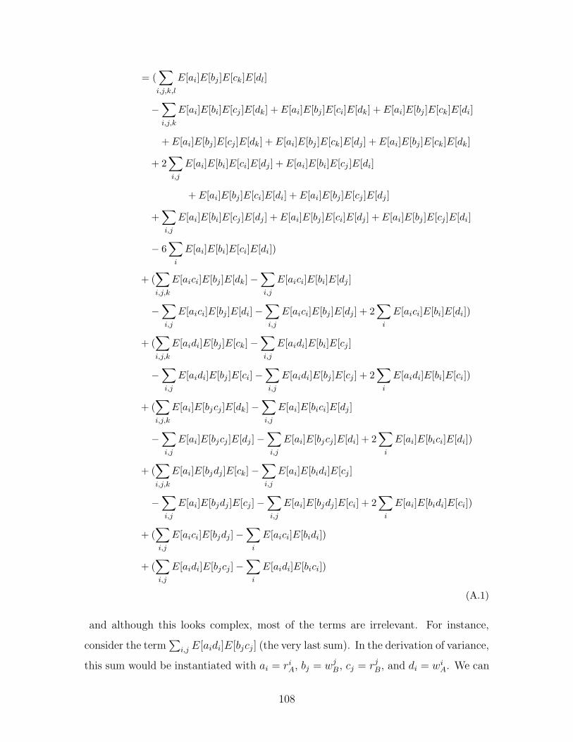
= (∑
i,j,k,l
E[ai]E[bj ]E[ck]E[dl]
−∑
i,j,k
E[ai]E[bi]E[cj ]E[dk] + E[ai]E[bj ]E[ci]E[dk] + E[ai]E[bj ]E[ck]E[di]
+ E[ai]E[bj ]E[cj ]E[dk] + E[ai]E[bj ]E[ck]E[dj ] + E[ai]E[bj ]E[ck]E[dk]
+ 2∑
i,j
E[ai]E[bi]E[ci]E[dj ] + E[ai]E[bi]E[cj ]E[di]
+ E[ai]E[bj ]E[ci]E[di] + E[ai]E[bj ]E[cj ]E[dj ]
+∑
i,j
E[ai]E[bi]E[cj ]E[dj ] + E[ai]E[bj ]E[ci]E[dj ] + E[ai]E[bj ]E[cj ]E[di]
− 6∑
i
E[ai]E[bi]E[ci]E[di])
+ (∑
i,j,k
E[aici]E[bj ]E[dk]−∑
i,j
E[aici]E[bi]E[dj ]
−∑
i,j
E[aici]E[bj ]E[di]−∑
i,j
E[aici]E[bj ]E[dj ] + 2∑
i
E[aici]E[bi]E[di])
+ (∑
i,j,k
E[aidi]E[bj ]E[ck]−∑
i,j
E[aidi]E[bi]E[cj ]
−∑
i,j
E[aidi]E[bj ]E[ci]−∑
i,j
E[aidi]E[bj ]E[cj ] + 2∑
i
E[aidi]E[bi]E[ci])
+ (∑
i,j,k
E[ai]E[bjcj ]E[dk]−∑
i,j
E[ai]E[bici]E[dj ]
−∑
i,j
E[ai]E[bjcj ]E[dj ]−∑
i,j
E[ai]E[bjcj ]E[di] + 2∑
i
E[ai]E[bici]E[di])
+ (∑
i,j,k
E[ai]E[bjdj ]E[ck]−∑
i,j
E[ai]E[bidi]E[cj ]
−∑
i,j
E[ai]E[bjdj ]E[cj ]−∑
i,j
E[ai]E[bjdj ]E[ci] + 2∑
i
E[ai]E[bidi]E[ci])
+ (∑
i,j
E[aici]E[bjdj ]−∑
i
E[aici]E[bidi])
+ (∑
i,j
E[aidi]E[bjcj ]−∑
i
E[aidi]E[bici])
(A.1)
and although this looks complex, most of the terms are irrelevant. For instance,
consider the term∑
i,j E[aidi]E[bjcj] (the very last sum). In the derivation of variance,
this sum would be instantiated with ai = riA, bj = wj
B, cj = rjB, and di = wi
A. We can
108
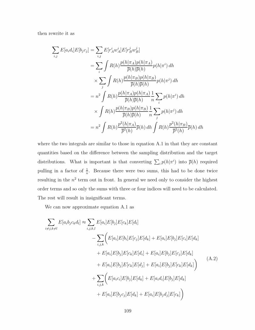
then rewrite it as
∑
i,j
E[aidi]E[bjcj] =∑
i,j
E[riAwi
A]E[rjBwj
B]
=∑
i
∫
R(h)p(h|πA)p(h|πA)
p(h)p(h)p(h|πi) dh
×∑
j
∫
R(h)p(h|πB)p(h|πB)
p(h)p(h)p(h|πj) dh
= n2
∫
R(h)p(h|πA)p(h|πA)
p(h)p(h)
1
n
∑
i
p(h|πi) dh
×
∫
R(h)p(h|πB)p(h|πB)
p(h)p(h)
1
n
∑
j
p(h|πj) dh
= n2
∫
R(h)p2(h|πA)
p2(h)p(h) dh
∫
R(h)p2(h|πB)
p2(h)p(h) dh
where the two integrals are similar to those in equation A.1 in that they are constant
quantities based on the difference between the sampling distribution and the target
distributions. What is important is that converting∑
i p(h|πi) into p(h) required
pulling in a factor of 1n. Because there were two sums, this had to be done twice
resulting in the n2 term out in front. In general we need only to consider the highest
order terms and so only the sums with three or four indices will need to be calculated.
The rest will result in insignificant terms.
We can now approximate equation A.1 as
∑
i6=j,k 6=l
E[aibjckdl] ≈∑
i,j,k,l
E[ai]E[bj]E[ck]E[dl]
−∑
i,j,k
(
E[ai]E[bi]E[cj]E[dk] + E[ai]E[bj]E[ci]E[dk]
+ E[ai]E[bj]E[ck]E[di] + E[ai]E[bj]E[cj]E[dk]
+ E[ai]E[bj]E[ck]E[dj] + E[ai]E[bj]E[ck]E[dk]
)
+∑
i,j,k
(
E[aici]E[bj ]E[dk] + E[aidi]E[bj]E[dk]
+ E[ai]E[bjcj]E[dk] + E[ai]E[bjdj]E[ck]
)
(A.2)
109
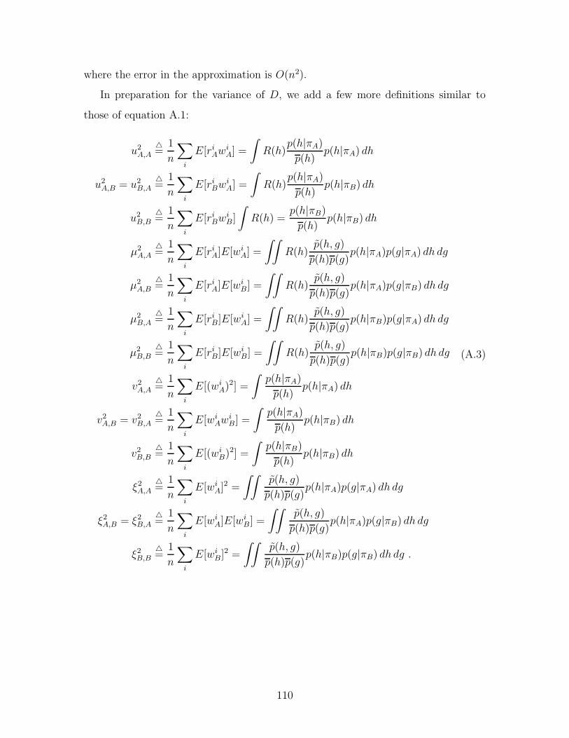
where the error in the approximation is O(n2).
In preparation for the variance of D, we add a few more definitions similar to
those of equation A.1:
u2A,A
4=
1
n
∑
i
E[riAwi
A] =
∫
R(h)p(h|πA)
p(h)p(h|πA) dh
u2A,B = u2
B,A
4=
1
n
∑
i
E[riBwi
A] =
∫
R(h)p(h|πA)
p(h)p(h|πB) dh
u2B,B
4=
1
n
∑
i
E[riBwi
B]
∫
R(h) =p(h|πB)
p(h)p(h|πB) dh
µ2A,A
4=
1
n
∑
i
E[riA]E[wi
A] =
∫∫
R(h)p(h, g)
p(h)p(g)p(h|πA)p(g|πA) dh dg
µ2A,B
4=
1
n
∑
i
E[riA]E[wi
B] =
∫∫
R(h)p(h, g)
p(h)p(g)p(h|πA)p(g|πB) dh dg
µ2B,A
4=
1
n
∑
i
E[riB]E[wi
A] =
∫∫
R(h)p(h, g)
p(h)p(g)p(h|πB)p(g|πA) dh dg
µ2B,B
4=
1
n
∑
i
E[riB]E[wi
B] =
∫∫
R(h)p(h, g)
p(h)p(g)p(h|πB)p(g|πB) dh dg
v2A,A
4=
1
n
∑
i
E[(wiA)2] =
∫
p(h|πA)
p(h)p(h|πA) dh
v2A,B = v2
B,A
4=
1
n
∑
i
E[wiAwi
B] =
∫
p(h|πA)
p(h)p(h|πB) dh
v2B,B
4=
1
n
∑
i
E[(wiB)2] =
∫
p(h|πB)
p(h)p(h|πB) dh
ξ2A,A
4=
1
n
∑
i
E[wiA]2 =
∫∫
p(h, g)
p(h)p(g)p(h|πA)p(g|πA) dh dg
ξ2A,B = ξ2
B,A
4=
1
n
∑
i
E[wiA]E[wi
B] =
∫∫
p(h, g)
p(h)p(g)p(h|πA)p(g|πB) dh dg
ξ2B,B
4=
1
n
∑
i
E[wiB]2 =
∫∫
p(h, g)
p(h)p(g)p(h|πB)p(g|πB) dh dg .
(A.3)
110
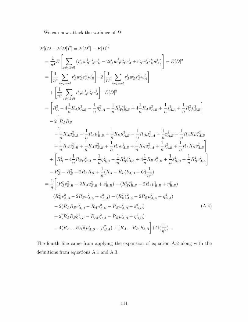
We can now attack the variance of D.
E[(D − E[D])2] = E[D2]− E[D]2
=1
n4E
[
∑
i6=j,k 6=l
(
riAwj
BrkAwl
B − 2riAwj
BrkBwl
A + riBwj
ArkBwl
A
)
]
− E[D]2
=
[
1
n4
∑
i6=j,k 6=l
riAwj
BrkAwl
B
]
−2
[
1
n4
∑
i6=j,k 6=l
riAwj
BrkBwl
A
]
+
[
1
n4
∑
i6=j,k 6=l
riBwj
ArkBwl
A
]
−E[D]2
=
[
R2A − 4
1
nRAµ2
A,B −1
nη2
A,A −1
nR2
Aξ2B,B + 4
1
nRAu2
A,B +1
ns2
A,A +1
nR2
Av2B,B
]
− 2
[
RARB
−1
nRAµ2
B,A −1
nRAµ2
B,B −1
nRBµ2
A,B −1
nRBµ2
A,A −1
nη2
A,B −1
nRARBξ2
A,B
+1
nRAu2
A,B +1
nRAu2
B,B +1
nRBu2
A,B +1
nRBu2
A,A +1
ns2
A,B +1
nRARBv2
A,B
]
+
[
R2B − 4
1
nRBµ2
B,A −1
nη2
B,B −1
nR2
Bξ2A,A + 4
1
nRBu2
A,B +1
ns2
B,B +1
nR2
Bv2A,A
]
−R2A −R2
B + 2RARB +1
n(RA −RB)bA,B + O(
1
n2)
=1
n
[
(R2Av2
B,B − 2RAu2B,B + s2
B,B)− (R2Aξ2
B,B − 2RAµ2B,B + η2
B,B)
(R2Bv2
A,A − 2RBu2A,A + s2
A,A)− (R2Bξ2
A,A − 2RBµ2A,A + η2
A,A)
− 2(RARBv2A,B − RAu2
A,B −RBu2A,B + s2
A,B)
+ 2(RARBξ2A,B −RAµ2
B,A −RBµ2A,B + η2
A,B)
− 4(RA −RB)(µ2A,B − µ2
B,A) + (RA − RB)bA,B
]
+O(1
n2) .
(A.4)
The fourth line came from applying the expansion of equation A.2 along with the
definitions from equations A.1 and A.3.
111
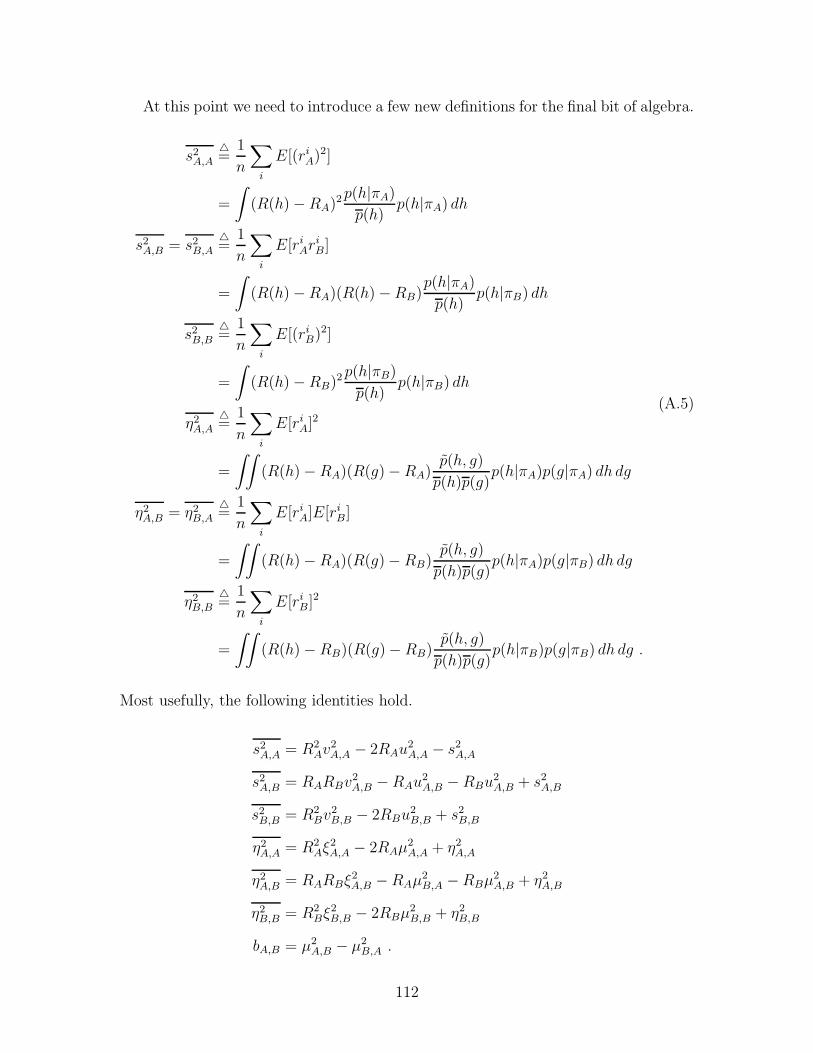
At this point we need to introduce a few new definitions for the final bit of algebra.
s2A,A
4=
1
n
∑
i
E[(riA)2]
=
∫
(R(h)−RA)2p(h|πA)
p(h)p(h|πA) dh
s2A,B = s2
B,A
4=
1
n
∑
i
E[riAri
B]
=
∫
(R(h)−RA)(R(h)−RB)p(h|πA)
p(h)p(h|πB) dh
s2B,B
4=
1
n
∑
i
E[(riB)2]
=
∫
(R(h)−RB)2 p(h|πB)
p(h)p(h|πB) dh
η2A,A
4=
1
n
∑
i
E[riA]2
=
∫∫
(R(h)− RA)(R(g)− RA)p(h, g)
p(h)p(g)p(h|πA)p(g|πA) dh dg
η2A,B = η2
B,A
4=
1
n
∑
i
E[riA]E[ri
B]
=
∫∫
(R(h)− RA)(R(g)− RB)p(h, g)
p(h)p(g)p(h|πA)p(g|πB) dh dg
η2B,B
4=
1
n
∑
i
E[riB]2
=
∫∫
(R(h)− RB)(R(g)− RB)p(h, g)
p(h)p(g)p(h|πB)p(g|πB) dh dg .
(A.5)
Most usefully, the following identities hold.
s2A,A = R2
Av2A,A − 2RAu2
A,A − s2A,A
s2A,B = RARBv2
A,B − RAu2A,B − RBu2
A,B + s2A,B
s2B,B = R2
Bv2B,B − 2RBu2
B,B + s2B,B
η2A,A = R2
Aξ2A,A − 2RAµ2
A,A + η2A,A
η2A,B = RARBξ2
A,B −RAµ2B,A −RBµ2
A,B + η2A,B
η2B,B = R2
Bξ2B,B − 2RBµ2
B,B + η2B,B
bA,B = µ2A,B − µ2
B,A .
112
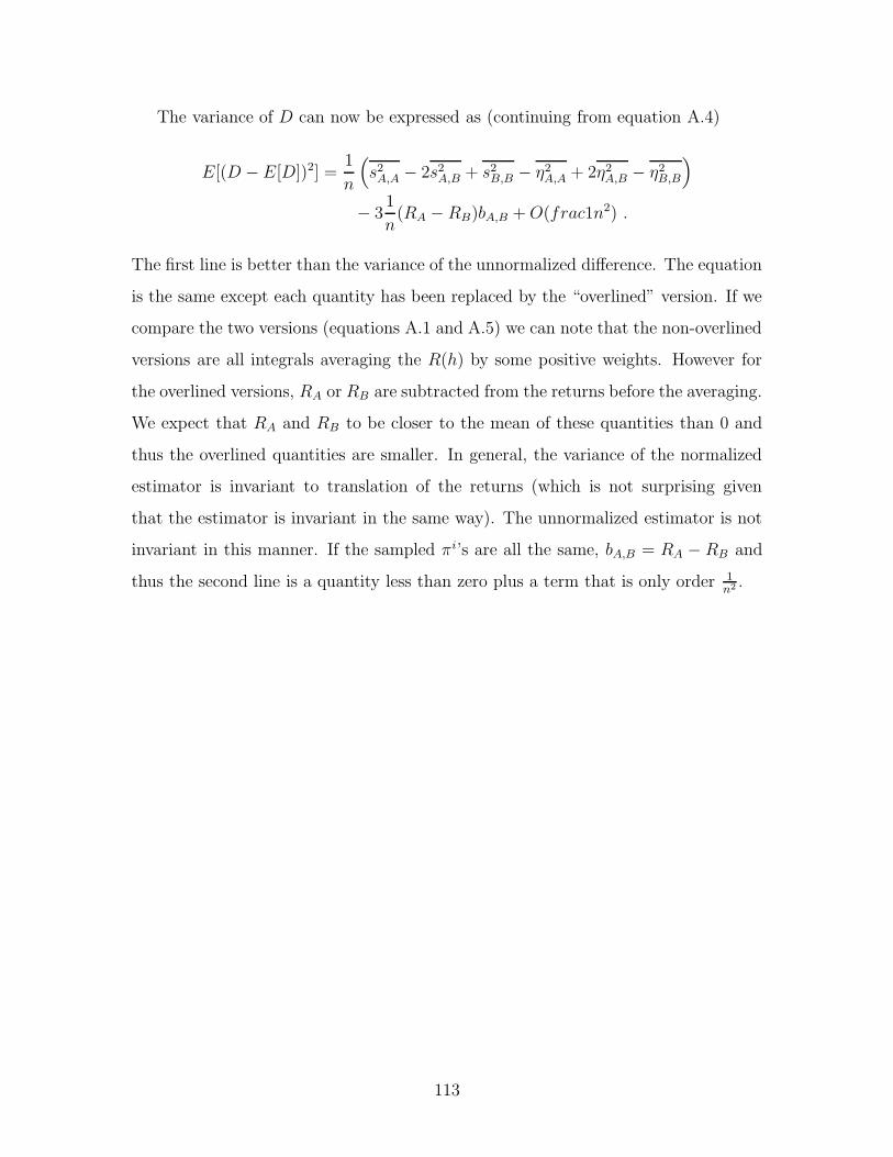
The variance of D can now be expressed as (continuing from equation A.4)
E[(D − E[D])2] =1
n
(
s2A,A − 2s2
A,B + s2B,B − η2
A,A + 2η2A,B − η2
B,B
)
− 31
n(RA − RB)bA,B + O(frac1n2) .
The first line is better than the variance of the unnormalized difference. The equation
is the same except each quantity has been replaced by the “overlined” version. If we
compare the two versions (equations A.1 and A.5) we can note that the non-overlined
versions are all integrals averaging the R(h) by some positive weights. However for
the overlined versions, RA or RB are subtracted from the returns before the averaging.
We expect that RA and RB to be closer to the mean of these quantities than 0 and
thus the overlined quantities are smaller. In general, the variance of the normalized
estimator is invariant to translation of the returns (which is not surprising given
that the estimator is invariant in the same way). The unnormalized estimator is not
invariant in this manner. If the sampled πi’s are all the same, bA,B = RA − RB and
thus the second line is a quantity less than zero plus a term that is only order 1n2 .
113

114
Bibliography
Amihud, Y. and H. Mendelson (1980). Dealership market: Market-making withinventory. Journal of Financial Economics 8, 31–53.
Anderson, B. S., A. W. Moore, and D. Cohn (2000). A nonparametric approach tonoisy and costly optimization. In Proceedings of the Seventeenth International
Conference on Machine Learning, pp. 17–24. Morgan Kaufmann.
Baird, L. and A. Moore (1999). Gradient descent for general reinforcement learning.In M. S. Kearns, S. A. Solla, and D. A. Cohn (Eds.), Advances in Neural
Information Processing Systems, Volume 11, pp. 968–974. The MIT Press.
Bengio, Y. (1999). Markovian models for sequential data. Neural Computing Sur-
veys 2, 129–162.
Bertsekas, D. P. and J. N. Tsitsiklis (1996). Neuro-Dynamic Programming. AthenaScientific.
Bishop, C. M. (1995). Neural Networks for Pattern Recognition. Oxford: ClarendonPress.
Box, G. E. P. and N. R. Draper (1987). Empirical Model-building and Response
Surfaces. Wiley.
Boyan, J. A. and A. W. Moore (1995). Generalization in reinforcement learning:Safely approximating the value function. In G. Tesauro, D. Touretzky, andT. Leen (Eds.), Advances in Neural Information Processing Systems, Volume 7,pp. 369–376. The MIT Press.
Chan, N. T. and C. Shelton (2001, April). An electronic market-maker. TechnicalReport AI-MEMO 2001-005, MIT, AI Lab.
Gabor, Z., Z. Kalmar, and C. Szepesvari (1998). Multi-criteria reinforcement learn-ing. In Proceedings of the Fifteenth International Conference on Machine Learn-
ing, pp. 197–205. Morgan Kaufmann.
Garman, M. (1976). Market microstructure. Journal of Financial Economics 3,257–275.
Geibel, P. (2001). Reinforcement learning with bounded risk. In Proceedings of
the Eighteenth International Conference on Machine Learning, pp. 162–169.Morgan Kaufmann.
Geweke, J. (1989, November). Bayesian inference in econometric models usingmonte carlo integration. Econometrica 57 (6), 1317–1339.
115
Glosten, L. R. and P. R. Milgrom (1985). Bid, ask and transaction prices in aspecialist market with heterogeneously informed traders. Journal of Financial
Economics 14, 71–100.
Gordon, G. J. (2001). Reinforcement learning with function approximation con-verges to a region. In T. K. Leen, T. G. Dietterich, and V. Tresp (Eds.), Ad-
vances in Neural Information Processing Systems, Volume 13, pp. 1040–1046.
Green, J. R. and J.-J. Laffont (1979). Incentives in Public Decision-Making. North-Holland Publishing Company.
Hesterberg, T. (1995). Weighted average importance sampling and defensive mix-ture distributions. Technometrics 37 (2), 185–194.
Ho, T. and H. R. Stoll (1981). Optimal dealer pricing under transactions and returnuncertainty. Journal of Financial Economics (9), 37–73.
Ho, T. and H. R. Stoll (1983). The dynamics of dealer markets under competition.Journal of Finance 38, 1053–1074.
Jaakkola, T., S. P. Singh, and M. I. Jordan (1995). Reinforcement learning algo-rithm for partially observable markov decision problems. In G. Tesauro, D. S. T.Touretzky, and T. K. Leen (Eds.), Advances in Neural Information Processing
Systems, Volume 7, pp. 345–352. The MIT Press.
Jordan, M. I. (Ed.) (1999). Learning in Graphics Models. Cambridge, MA: TheMIT Press.
Kaelbling, L. P. (2001, June). oral presentation in the hierarchy and memory work-shop at the Eighteenth International Conference on Machine Learning.
Kaelbling, L. P., M. L. Littman, and A. W. Moore (1996). Reinforcement learning:A survey. Journal of Artificial Intelligence Research 4, 237–285.
Kearns, M., Y. Mansour, and A. Ng (2000). Approximate planning in largePOMDPs via reusable trajectories. In S. A. Solla, T. K. Leen, and K.-R. Muller(Eds.), Advances in Neural Information Processing Systems, Volume 12, pp.1001–1007.
Kloek, T. and H. K. van Dijk (1978, January). Bayesian estimates of equationsystem parameters: An application of integration by monte carlo. Economet-
rica 46 (1), 1–19.
Konda, V. R. and J. N. Tsitsiklis (2000). Actor-critic algorithms. In S. A. Solla,T. K. Leen, and K.-R. Muller (Eds.), Advances in Neural Information Process-
ing Systems, Volume 12, pp. 1008–1014. The MIT Press.
Littman, M. (1996). Algorithms for Sequential Decision Making. Ph. D. thesis,Brown University.
Lock, J. and S. Singh (1998). Using eligibility traces to find the best memorylesspolicy in partially observable markov decision processes. In Proceedings of the
Fifteenth International Conference on Machine Learning, pp. 141–150. MorganKaufmann.
116
Mas-Collel, A., W. Whinston, and J. Green (1995). Microeconomic Theory. OxfordUniversity Press.
McAllester, D. (2000, December). personal communication.
Meuleau, N., L. Peshkin, and K.-E. Kim (2001, April). Exploration in gradient-based reinforcement learning. Technical Report AI-MEMO 2001-003, MIT, AILab.
Meuleau, N., L. Peshkin, K.-E. Kim, and L. P. Kaelbling (1999). Learning finite-state controllers for partially observable environments. In Proceedings of the
Fifteenth International Conference on Uncertainty in Artificial Intelligence.
Moore, A. W., J. Schneider, J. Boyan, and M. S. Lee (1998). Q2: A memory-basedactive learning algorithm for blackbox noisy optimization. In Proceedings of the
Fifteenth International Conference on Machine Learning, pp. 386–394. MorganKaufmann.
Ng, A. Y. and M. Jordan (2000). Pegasus: A policy search method for large MDPsand POMDPs. In Proceedings of the Sixteenth International Conference on Un-
certainty in Artificial Intelligence.
O’Hara, M. and G. Oldfield (1986, December). The microeconomics of marketmaking. Journal of Financial and Quantitative Analysis 21, 361–376.
Peshkin, L., N. Meuleau, and L. P. Kaelbling (1999). Learning policies with externalmemory. In Proceedings of the Sixteenth International Conference on Machine
Learning. Morgan Kaufmann.
Peshkin, L. and S. Mukherjee (2001). Bounds on sample size for policy evaluationin markov environments. In Fourteenth Annual Conference on Computational
Learning Theory.
Precup, D., R. S. Sutton, and S. Dasgupta (2001). Off-policy temporal-differencelearning with function approximation. In Proceedings of the Eighteenth Inter-
national Conference on Machine Learning. Morgan Kaufmann.
Precup, D., R. S. Sutton, and S. Singh (2000). Eligibility traces for off-policypolicy evaluation. In Proceedings of the Seventeenth International Conference
on Machine Learning. Morgan Kaufmann.
Press, W. H., S. A. Teukolsky, W. T. Vetterling, and B. P. Flannery (1992). Nu-
merical Recipes in C (Second ed.). Cambridge University Press.
Rabiner, L. R. (1989, February). A tutorial on hidden markov models and selectedapplications in speech recognition. Proceedings of the IEEE 77 (2), 257–286.
Resnik, M. D. (1987). Choices: An Introduction to Decision Theory. University ofMinnesota Press.
Rubinstein, R. Y. (1981). Simulation and the Monte Carlo Method. John Wiley &Sons.
Scholkopf, B., C. J. Burges, and A. J. Smola (Eds.) (1999). Advances in Kernel
Methods. Cambridge, MA: The MIT Press.
117
Shelton, C. R. (2001). Balancing multiple sources of reward in reinforcement learn-ing. In T. K. Leen, T. G. Dietterich, and V. Tresp (Eds.), Advances in Neural
Information Processing Systems, Volume 13, pp. 1082–1088.
Sutton, R. S. and A. G. Barto (1998). Reinforcement Learning: An Introduction.The MIT Press.
Sutton, R. S., D. McAllester, S. Singh, and Y. Mansour (2000). Policy gradi-ent methods for reinforcement learning with function approximation. In S. A.Solla, T. K. Leen, and K.-R. Muller (Eds.), Advances in Neural Information
Processing Systems, Volume 12, pp. 1057–1063. The MIT Press.
Williams, J. K. and S. Singh (1999). Experimental results on learning stochasticmemoryless policies for partially observable markov decision processes. In M. S.Kearns, S. A. Solla, and D. A. Cohn (Eds.), Advances in Neural Information
Processing Systems, Volume 11, pp. 1073–1079.
Williams, R. J. (1992). Simple statistical gradient-following algorithms for connec-tionist reinforcement learning. Machine Learning 8, 229–256.
118