Embed Size (px)
Citation preview
Implicit partitioned Runge-Kutta integratorsfor simulations of gauge theories
Master Thesis
Master’s ProgramComputer Simulation in Science
Supervisors:
Prof. Dr. Michael GuntherProf. Dr. Francesco Knechtli
Michele WandeltFaculty of Mathematics and Natural Science
University of Wuppertal
April 30, 2010


Contents
Introduction 1
1 Gauge Fields on a Lattice 31.1 Gauge Field . . . . . . . . . . . . . . . . . . . . . . . . . . . . . 41.2 Wilson Action . . . . . . . . . . . . . . . . . . . . . . . . . . . . 61.3 Hamilton Operator . . . . . . . . . . . . . . . . . . . . . . . . . 71.4 Hamiltonian Equations of Motion . . . . . . . . . . . . . . . . . 8
1.4.1 Time Derivatives of the Links . . . . . . . . . . . . . . . 81.4.2 Time Derivatives of the Momenta . . . . . . . . . . . . . 10
2 Hybrid Monte Carlo Method 152.1 Metropolis Monte Carlo Method . . . . . . . . . . . . . . . . . . 15
2.1.1 Markov Process . . . . . . . . . . . . . . . . . . . . . . . 162.1.2 Metropolis Algorithm . . . . . . . . . . . . . . . . . . . . 17
2.2 Hybrid Monte Carlo Method . . . . . . . . . . . . . . . . . . . . 18
3 Numerical Integration 233.1 Desired Properties of the Integration Scheme . . . . . . . . . . . 24
3.1.1 Differential Equations on Lie Groups . . . . . . . . . . . 243.1.2 Symmetry (= Time-Reversibility) . . . . . . . . . . . . . 263.1.3 Convergence Order . . . . . . . . . . . . . . . . . . . . . 26
3.2 The Stormer-Verlet (= Leapfrog) Method . . . . . . . . . . . . . 273.2.1 Lie-Euler Method . . . . . . . . . . . . . . . . . . . . . . 273.2.2 Stormer-Verlet Method . . . . . . . . . . . . . . . . . . . 29
3.3 Partitioned Runge-Kutta Methods for Lie Groups . . . . . . . . 303.3.1 Partitioned Runge-Kutta Methods in General . . . . . . 303.3.2 Munthe-Kaas Method . . . . . . . . . . . . . . . . . . . 323.3.3 Conditions of Symmetry (= Time-Reversibility) . . . . . 343.3.4 Derivation of the Order Conditions . . . . . . . . . . . . 38
3.4 Munthe-Kaas Method for Convergence Order 2 and 3 . . . . . . 383.4.1 Symmetric Partitioned Runge-Kutta Method of Order 2 393.4.2 Symmetric Partitioned Runge-Kutta Method of Order 3 42
4 Simulation 494.1 Model: An SU(2,C) Lattice Gauge Field . . . . . . . . . . . . . 494.2 Details of the Simulation . . . . . . . . . . . . . . . . . . . . . . 524.3 Results . . . . . . . . . . . . . . . . . . . . . . . . . . . . . . . . 53
i

4.3.1 Model of a 4x4-Lattice with β = 2.0 . . . . . . . . . . . . 534.3.2 Volume Dependence . . . . . . . . . . . . . . . . . . . . 574.3.3 Dependence on the Gauge Coupling β . . . . . . . . . . 59
Conclusion and outlook 59
A Theory 65
B Calculations 67B.1 Check of the symmetry and the convergence order 2 . . . . . . . 67
ii
List of Figures
1.1 Lattice sites . . . . . . . . . . . . . . . . . . . . . . . . . . . . . 31.2 Lattice links . . . . . . . . . . . . . . . . . . . . . . . . . . . . . 41.3 Links in forward and backward direction . . . . . . . . . . . . . 41.4 Plaquette . . . . . . . . . . . . . . . . . . . . . . . . . . . . . . 51.5 Staples of a link . . . . . . . . . . . . . . . . . . . . . . . . . . . 5
4.1 Convergence order . . . . . . . . . . . . . . . . . . . . . . . . . 544.2 Acceptance rate . . . . . . . . . . . . . . . . . . . . . . . . . . . 554.3 Expectation value of the mean plaquette value . . . . . . . . . . 554.4 Expectation value of exp(−∆H) . . . . . . . . . . . . . . . . . . 564.5 Number of fixed point iterations per integration step . . . . . . 574.6 Mean time consumption per trajectory per link . . . . . . . . . 574.7 Volume dependence: Convergence orders . . . . . . . . . . . . . 584.8 Volume dependence: Expectation value of exp(−∆H) . . . . . . 584.9 Volume dependence: Number of fixed point iterations per inte-
gration step . . . . . . . . . . . . . . . . . . . . . . . . . . . . . 594.10 Volume dependence: Computational time . . . . . . . . . . . . . 594.11 Volume dependence: Comparison of the computational time at
a similar acceptance rate . . . . . . . . . . . . . . . . . . . . . . 604.12 Dependence on the gauge coupling term β: Convergence order . 604.13 Dependence on the gauge coupling term β: Computational time 61
iii

iv

List of Tables
3.1 Coefficients of the partitioned Runge-Kutta method followingthe Leapfrog method . . . . . . . . . . . . . . . . . . . . . . . . 42
3.2 Coefficients of the partitioned Runge-Kutta method of conver-gence order 3 . . . . . . . . . . . . . . . . . . . . . . . . . . . . 47
4.1 Comparison of the computational time at a similar acceptancerate . . . . . . . . . . . . . . . . . . . . . . . . . . . . . . . . . 56
v


Acknowledgement
First of all, I would like to thank my supervisors Prof. Dr. Michael Guntherand Prof. Dr. Francesco Knechtli for the idea of this interesting interdisci-plinary Master Thesis. Your doors were opened at any time and I am gratefulfor your continual support.
Additionally, I would like to send a warm thanks to Dr. Michael Striebel forthe proofreading of this work.
Furthermore, a special thank goes to Matthias Lichter for the introduction inthe secrets of Matlab and especially Mathematica. Without Mathematica, Iwould have been lost in the calculation of the method coefficients.
Wuppertal, April 2010 Michele Wandelt


Introduction
In the simulations of gauge theories, expectation values of certain operatorshave to be calculated. This is usually performed using a Hybrid Monte Carlomethod that combines a Metropolis step with a Molecular Dynamics step.During the Molecular Dynamics step, Hamiltonian equations of motion haveto be solved through an integration scheme. The state-of-the-art integrationmethods are the Leapfrog scheme as well as spliting methods.
At the beginning of this thesis, there was the question:
• Are there any higher order numerical integration schemes besides theLeapfrog or splitting methods for simulations of gauge theories?
For this to be possible, it has to be taken into account that the numericalintegration method has to fulfill some desired properties. First of all, it has tobe symmetric, i. e. time reversible and of a preferably high convergence order.Due to the fact that the intgration method has to be applied in gauge theorieswith elements regarded to be situated in a Lie group, the preservation of theLie group structure has to be fulfilled as well.As mentioned in the title of this thesis, implicit partitioned Runge-Kutta meth-ods are chosen to be examined in this work.
In chapter 1, a lattice gauge theory is introduced. It is described from a math-ematical point of view with respect to the simulations.The necessary conceptsas link, plaquette and staple are depicted here. Additionally, the Hamiltonoperator and the derivation of its equations of motion are outlined.
Chapter 2 describes the Markov process used in a Metropolis method. More-over, the Hybrid Monte Carlo algorithm is characterized in detail. The neces-sity of the properties symmetry and symplecticity (=volume-preservation) ofthe numerical intergration scheme are discussed. These features are used inthe detailed balance condition of the Markov process to ensure the reachabilityof the equilibrium distribution of the field.
The numerical integration is the main part of this thesis and situated in chapter3. It starts with an examination of the aforementioned desired properties. Thecharacteristics symmetry and convergence order are described and connectedto well-known integration schemes including the Leapfrog method. (The men-tioned splitting methods are not investigated here, they can be found in [1].)
1

Furthermore, some facts on differential equations on Lie groups are carriedtogether.Considering the aforementioned properties, partitioned Runge-Kutta methodsfor Lie groups are developed. During this process, there arise some difficul-ties: First of all, the solution of the differential equations of course has to bean element of the Lie group. This is achieved using a Munthe-Kaas methodwhich replaces the differential equation in the Lie group through a differentialequation in the appropriate Lie algebra and maps the result back in the Liegroup via an exponential function. In this process, the differential equation isreplaced by a truncated series which depends on the desired convergence order.Moreover, the integration method has to be symmetric. Due to the shape ofthe previously described mapping, this is none too easy. There occur problemsconcerning the exponential function in the mapping, such that an additionalterm is needed. Finally, the convergence order of the partitioned Runge-Kuttamethod is derived via Taylor expansions. Since the differential equation is asuitable truncation of a series, this has to be done for each desired convergenceorder separately. At the end of this chapter, there are two symmetric implicitpartitioned Runge-Kutta methods with appropriate conditions for the symme-try and its convergence orders 2 and 3 derived. For the executed simulations,there are values for the coefficients needed. The coefficients for convergenceorder 2 are taken from [2]. For convergence order 3, they are chosen accord-ing to calculations performed with the computer algebra system Mathematica.
In chapter 4, the details of the model of an SU(2,C) lattice gauge field aredescribed. Then, the used fixed point iterations are discussed. In the lastparagraph, the results of the executed simulations are presented which indicate,that a convergence order 4 can be achieved. These simulations are performedusing the software package Matlab. For the investigation of the derived Runge-Kutta method, a lattice of size 4 × 4 with gauge coupling β = 2.0 is chosen.Furthermore, the dependence on the lattice volume and the gauge couplingare examined.
2

Chapter 1
Gauge Fields on a Lattice
The first chapter serves as a rough introduction to gauge fields on a lattice.The necessary information for understanding the numerical simulations willbe provided here. Thereby, the sections concerning the gauge field and theWilson action are described in [3] and [4]. Parts of section 1.3 can be found in[5].
Figure 1.1: Lattice sites [x]. The field [ϕ] on a discrete lattice [x] is given. Itcan be imagined as a color space at the sites x.
Let a field [ϕ] on a discrete lattice [x] be given.One of the fundamental objects of quantum field theory is the calculation ofthe expectation value ⟨A⟩ of some operator A
([ϕ]). This is done via a path
integral of the lattice action S([ϕ])
⟨A⟩ = 1Z
∫[dϕ] exp
(−S
([ϕ]))
A([ϕ])
(1.1)
with partition function
Z =∫
[dϕ] exp(−S
([ϕ])),
integration measure [dϕ], and lattice action S([ϕ]). The lattice action S
([ϕ])
has to fulfill two conditions. It must reach the correct continuum limit and hasto be gauge invariant. This will be described more detailed in the followingpragraphs.
3

Chapter 1. Gauge Fields on a Lattice
1.1 Gauge FieldLet an equidistant lattice with lattice spacing a and periodic boundary condi-tions be given. We introduce a gauge field [U ] that is a set of matrices beingelements of the special unitary Lie group SU(N,C).
SU(N,C) = X ∈ Gl(N,C) : X† = X−1 and det(X) = 1.
The matrices Ux,µ of the set [U ] represent the links between two adjacent latticesites from site x in direction µ and are shown as arrows in figure 1.2.
µ = 0
µ = 1 a
Figure 1.2: 2-dimensional field [U ] of lattice links on an equidistant latticewith lattice spacing a and periodic boundary conditions. The orientation isgiven as µ = 0, 1.
Definition 1.1 (Link matrices). A matrix
Ux,µ ∈ SU(N,C)
is called link matrix. It is situated on the link from the lattice site x to its nextneighbour x + aµ in direction µ = 0, 1 and will be shortly referred as link.µ denotes the unit vector in direction µ, such that 0 = (1, 0)T and 1 = (0, 1)Tholds. The vector µ is scaled by the lattice constant a.
A link is orientated such that Ux,µ can be seen as a forward connection. Thusthe link Ux+aµ,−µ from site x + aµ in the reverse direction −µ is a backwardconnection. They are related through Ux+aµ,−µ = U †
x,µ since the backwardconnection is simply the reversed forward one.
x x + aµ
U †x,µ = Ux+aµ,−µ
x x + aµ
Ux,µ
Figure 1.3: Left: Link Ux,µ from site x in direction µ. Right: Link U †x,µ in the
reverse direction (from site x+ aµ in direction −µ).
4

1.1. Gauge Field
Definition 1.2 (Plaquette variable). The plaquette variable
U01(x) = Ux,01 := Ux,0Ux+a0,1U†x+a1,0U
†x,1 (1.2)
related to site x in the (0, 1)-plane is the smallest closed loop of link matricesin counterclockwise direction. It is defined as the product over contiguous linkmatrices starting and ending at site x and also called plaquette.
Ux,0
Ux+a0,1
U†x+a1,0
U†x,1
x
Figure 1.4: The plaquette is the shortest closed loop on the lattice.
Besides the plaquette, the staple is another important notation in quantumfield theories. For every link Ux,µ from site x to site x+aµ there exist shortestpaths from site x+ aµ to site x not containing the link itself. These paths arecalled staples of the link Ux,µ.
Ux,0
Ux−a1,1Ux+a0,1
Ux,0
U†x−a1,0
U†x+a1,0
U†x,1 U†
x+a(0−1),1
Figure 1.5: Staples of the link Ux,µ.
Definition 1.3 (Staples). The sum of all shortest paths is called sum of staplesand will be denoted with Vx,µ := V (Ux,µ). The sum of staples belonging to thelink Ux,0, respective link Ux,1 are
Vx,0 := V (Ux,0) = Ux+a0,1U†x+a1,0U
†x,1 + U †
x+a(0−1),1U†x−a1,0Ux−a1,1
resp. Vx,1 := V (Ux,1) = Ux+a1,0U†x+a0,1U
†x,0 + U †
x+a(1−0),0U†x−a0,1Ux−a0,0
5

Chapter 1. Gauge Fields on a Lattice
1.2 Wilson ActionThe lattice action has to be gauge invariant. In this paragraph, we introducethe Wilson gauge action and show its gauge invariance. For this purpose, theexpression gauge transformation has to be explained.
Definition 1.4 (Gauge transformation). Let [W ] be a set of matrices Wx,
Wx ∈ SU(N,C),
situated on the lattice sites. The gauge transformation
ϕx → ϕ′x = Wxϕx.
rotates the elements of the color space [ϕ]. The link matrices are transformedas
Ux,µ → U ′x,µ = WxUx,µW
†x+aµ.
Thus the gauge inner product ϕ†(x)Ux,µϕ(x+ aµ) is invariant under the gaugetransformation because ϕ†xUx,µϕx+aµ transforms to
(ϕ′x)†U ′x,µϕ
′x+aµ =
(Wxϕx
)† ·WxUx,µW†x+aµ ·Wx+aµϕx+aµ
= ϕ†x ·W †xWx · Ux,µ ·W †
x+aµWx+aµ · ϕx+aµ
= ϕ†xUx,µϕx+aµ.
The Wilson action is the lattice action corresponding to the plaquettes. It willbe denoted as SG
([U ]
)in the following.
Definition 1.5 (Wilson action). The Wilson action
SG([U ]
)=∑
x
β
(1− 1
NRe(tr(U01(x)
)))(1.3)
depends on the sum of the real part of the trace of all plaquettes. Note thatthis sum contains every plaquette with just one orientation. The factor β is ahopping parameter and can be seen as inverse temperature.
Remark 1.6 (Gauge invariance of the Wilson action). The Wilson action isgauge invariant if SG
([U ]
)= SG
([U ′]
)holds.
Due to the fact that the Wilson action depend on the trace of the plaquette,the gauge invariance can be easily shown:
U ′01(x) = Ux,0Ux+a0,1U
†x+a1,0U
†x,1
= WxUx,0W†x+a0Wx+a0Ux+a0,1W
†x+a(0+1)
(Wx+a1Ux+a1,0W
†x+a(1+0)
)†(WxUx,1W
†x+a1
)†
= WxUx,0W†x+a0Wx+a0Ux+a0,1W
†x+a(0+1)Wx+a(1+0)U
†x+a1,0W
†x+a1Wx+a1U
†x,1W
†x
= WxUx,0Ux+a0,1U†x+a1,0U
†x,1W
†x
= WxU01(x)W †x .
6

1.3. Hamilton Operator
All except for the first and the last transformation matrices Wx vanish. Be-cause of the properties of the trace, the trace of a closed path of link variabesis gauge invariant.
tr(U ′
01(x))
= tr(WxU01(x)W †
x
)
= tr(W †
xWxU01(x))
= tr(U01(x)
).
Thus the Wilson action is gauge invariant. It is possible to create other gaugeinvariant expressions, for example by another closed path of links. For a smalllattice spacing a→ 0 the continuum limit will be reached.
Remark 1.7 (Expectation value of a gauge field). We can transfer the expec-tation value ⟨A⟩ of equation (1.1) to the one of a bosonic gauge field [U ] withWilson action SG
([U ]
). It reads
⟨A⟩ = 1Z
∫[dU ] exp
(SG([U ]
))A([U ]
)(1.4)
with Haar measure [dU ] (see definition A.1) and partition function
Z =∫
[dU ] exp(−SG
([U ]
)).
The expectation value ⟨A⟩ will be computed numerically. As we shall see later,we use a Hybrid Monte Carlo method to evaluate the path integral of equation(1.4). For this purpose, we need the Hamiltonian of the gauge field.
1.3 Hamilton OperatorThe Hamiltonian H represents the total energy of the bosonic field. It is aconserved quantity, such that its time derivative H vanishes. Furthermore,the Hamiltonian induces the Hamiltonian equations of motion.
Momenta
We introduce a field [P ] of fictious momenta on the lattice needed for thedefinition of the Hamiltonian. The momenta [P ] are associated with the links[U ]. For every link matrix Ux,µ there exists a fictitious conjugated momentumPx,µ. These elements Px,µ are traceless, and hermitian (N ×N)-matrices, i. e.
Px,µ = P †x,µ and tr
(Px,µ
)= 0.
The traceless and anti-hermitian matrices iPx,µ are elements of the Lie algebra
su(N,C) = X ∈ Gl(N) | X + X† = 0 and tr(X)
= 0.
associated to the Lie group SU(N,C).
7

Chapter 1. Gauge Fields on a Lattice
Definition 1.8. The Hamiltonian
H([U, P ]
)= Ekin
([P ])
+ SG([U ]
)(1.5)
depends on the set of link matrices [U ] and its conjugated momenta [P ]. Itconsists of the kinetic energy Ekin and the Wilson action SG.
The kinetic energy is associated with the set of momenta [P ] and reads
Ekin
([P ])
= 12∑
x
∑
µ=0,1tr(P 2x,µ
). (1.6)
The Hamilton operator induces the Hamiltonian equations of motion:
∂H([U, P ]
)
∂Ux,µ
= −∂Px,µ∂t
= −Px,µ
and∂H
([U, P ]
)
∂Px,µ= ∂Ux,µ
∂t= Ux,µ.
Note that the time derivatives Ux,µ and Px,µ do not depend on real time but ona fictious computer time. This means the Hamilton operator and its equationsof motion are quite artificial because the momenta and the time are factitious.Nevertheless, we can develop formulas to compute the Hamiltonian equationsof motion.
1.4 Hamiltonian Equations of MotionThe Hamiltonian equations of motion read
∂H([U, P ]
)
∂Px,µ= Ux,µ = iPx,µUx,µ (1.7)
and∂H
([U, P ]
)
∂Ux,µ
= −Px,µ = −i βN
Ux,µVx,µ
TA(1.8)
with traceless and anti-hermitian operatorUx,µVx,µ
TA= 1
2Wx,µ −1
2N tr(Wx,µ
)· IN . (1.9)
using Wx,µ = Ux,µVx,µ − V †x,µU
†x,µ. The variable Vx,µ is called sum of staples as
mentioned in definition 1.3.
1.4.1 Time Derivatives of the LinksThe differential equation
Ux,µ = iPx,µ · Ux,µ. (1.10)
8
1.4. Hamiltonian Equations of Motion
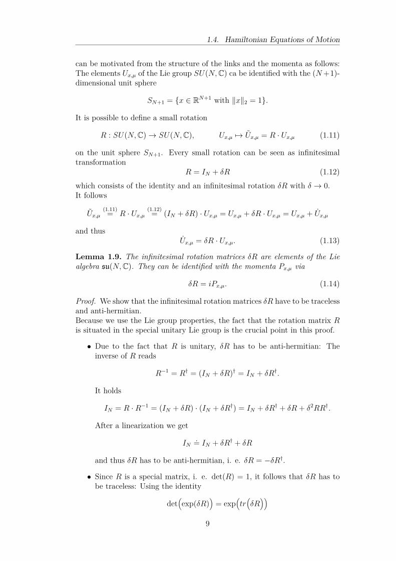
can be motivated from the structure of the links and the momenta as follows:The elements Ux,µ of the Lie group SU(N,C) ca be identified with the (N+1)-dimensional unit sphere
SN+1 = x ∈ RN+1 with ∥x∥2 = 1.
It is possible to define a small rotation
R : SU(N,C) → SU(N,C), Ux,µ 7→ Ux,µ = R · Ux,µ (1.11)
on the unit sphere SN+1. Every small rotation can be seen as infinitesimaltransformation
R = IN + δR (1.12)which consists of the identity and an infinitesimal rotation δR with δ → 0.It follows
Ux,µ(1.11)= R · Ux,µ
(1.12)= (IN + δR) · Ux,µ = Ux,µ + δR · Ux,µ = Ux,µ + Ux,µ
and thusUx,µ = δR · Ux,µ. (1.13)
Lemma 1.9. The infinitesimal rotation matrices δR are elements of the Liealgebra su(N,C). They can be identified with the momenta Px,µ via
δR = iPx,µ. (1.14)
Proof. We show that the infinitesimal rotation matrices δR have to be tracelessand anti-hermitian.Because we use the Lie group properties, the fact that the rotation matrix Ris situated in the special unitary Lie group is the crucial point in this proof.
• Due to the fact that R is unitary, δR has to be anti-hermitian: Theinverse of R reads
R−1 = R† = (IN + δR)† = IN + δR†.
It holds
IN = R ·R−1 = (IN + δR) · (IN + δR†) = IN + δR† + δR + δ2RR†.
After a linearization we get
IN.= IN + δR† + δR
and thus δR has to be anti-hermitian, i. e. δR = −δR†.
• Since R is a special matrix, i. e. det(R) = 1, it follows that δR has tobe traceless: Using the identity
det(exp(δR)
)= exp
(tr(δR))
9

Chapter 1. Gauge Fields on a Lattice
and the Taylor expansion
R = IN + δR + 12(δR)2
+ . . . = exp(δR)
of R, we get
1 = det(R) = det(exp(δR)
)= exp
(tr(δR)).
Hence, δR has to be traceless.
The equation of motionUx,µ = iPx,µ · Ux,µ. (1.10)
immediately follows from (1.13) and (1.14).
1.4.2 Time Derivatives of the MomentaThe derivation of the equation of motion for the momenta needs a few consid-erations: Due to the energy conservation, it holds
H([U, P ]
)= Ekin
([P ])
+ SG([U ]
)= 0.
Thus we have to deduce the time derivatives of the kinetic energy and theWilson action to get a concrete formula for H: While it is evident that
Ekin
([P ])
= 12∑
x
∑
µ=0,1tr(Px,µPx,µ + Px,µPx,µ
)
=∑
x
∑
µ=0,1tr(Px,µPx,µ
)(1.15)
holds, the calculation of the derivative of the Wilson action
SG([U ]
)= − β
2N∑
x
∑
µ=0,1tr(Ux,µVx,µ + V †
x,µU†x,µ
)(1.16)
requires some additional work.
The derivative of the Wilson action
We start with the Wilson action and use the property (A.4) of the trace:
SG([U ]
)=∑
x
β
(1− 1
NRe(tr(U01(x)
)))
=∑
x
β(1− 1
2N tr(U01(x) + U †
01(x))).
10
1.4. Hamiltonian Equations of Motion
Then, we replace the plaquette variable U01(x) with the product of links (seeequation (1.2)) and rewrite the Wilson action as
SG([U ]
)= − β
2N∑
x
(tr(Ux,0Ux+a0,1U
†x+a1,0U
†x,1 +
(Ux,0Ux+a0,1U
†x+a1,0U
†x,1
)†))
= − β
2N∑
x
(tr(Ux,0Ux+a0,1U
†x+a1,0U
†x,1 + Ux,1Ux+a1,0U
†x+a0,1U
†x,0
)).
The time derivative SG([U ]
)of the Wilson action can be computed in a
straightforward way. Because a reordering of the matrix product has no effecton the trace (see equation (A.3)), the time derivations of the links are placedat the beginning and the end of a product of links.
SG([U ]
)= − β
2N∑
x
tr(
Ux,0Ux+a0,1U†x+a1,0U
†x,1 + Ux,1Ux+a1,0U
†x+a0,1U
†x,0
+ Ux+a0,1U†x+a1,0U
†x,1Ux,0 + Ux+a1,0U
†x+a0,1U
†x,0Ux,1
+ U †x,1Ux,0Ux+a0,1U
†x+a1,0 + U †
x,0Ux,1Ux+a1,0U†x+a0,1
+ Ux,0Ux+a0,1U†x+a1,0U
†x,1 + Ux,1Ux+a1,0U
†x+a0,1U
†x,0
)(1.17)
Taking account of some additional information, we simplify this expression.Since we sum over all lattice sites x, we can shift some indices. This will bedone in such a way that we can factorise the time derivatives of the links, e.g.
x + a1, 0 → x, 0 and x + a0, 1 → x, 1.
The shifts in direction −0 and −1 imply the changes
x + a0, 1 −0−→ x, 1x + a1, 0 −0−→ x + a(1− 0), 0,
x, 1 −0−→ x− a0, 1,x, 0 −0−→ x− a0, 0,
x + a1, 0 −1−→ x, 0,x + a0, 1 −1−→ x + a(0− 1), 1,
x, 0 −1−→ x− a1, 0,x, 1 −1−→ x− a1, 1.
Using these shifts and equation (1.17), we get
∑
x
tr(Ux,0Ux+a0,1U
†x+a1,0U
†x,1 + Ux+a1,0U
†x+a0,1U
†x,0Ux,1
)
=∑
x
tr(Ux,0
(Ux+a0,1U
†x+a1,0U
†x,1 + U †
x+a(0−1),1U†x−a1,0Ux−a1,1
))
and∑
x
tr(Ux,1Ux+a1,0U
†x+a0,1U
†x,0 + Ux+a0,1U
†x+a1,0U
†x,1Ux,0
)
=∑
x
tr(Ux,1
(Ux+a1,0U
†x+a0,1U
†x,0 + U †
x+a(1−0),0U†x−a0,1Ux−a0,0
)).
11
Chapter 1. Gauge Fields on a Lattice
The inner sums of the expressions above consist of the sum of staples of thelinks Ux,0 and Ux,1. This implies
∑
x
tr(Ux,0Ux+a0,1U
†x+a1,0U
†x,1 + Ux+a1,0U
†x+a0,1U
†x,0Ux,1
)=∑
x
tr(Ux,0Vx,0
)
and∑
x
tr(Ux,1Ux+a1,0U
†x+a0,1U
†x,0 + Ux+a0,1U
†x+a1,0U
†x,1Ux,0
)=∑
x
tr(Ux,1Vx,1
).
The other 4 addends of equation (1.17) lead to the inverse expressions∑
x
tr(U †x,1Ux,0Ux+a0,1U
†x+a1,0 + Ux,1Ux+a1,0U
†x+a0,1U
†x,0
)=∑
x
tr(V †x,0U
†x,0
)
and∑
x
tr(U †x,0Ux,1Ux+a1,0U
†x+a0,1 + Ux,0Ux+a0,1U
†x+a1,0U
†x,1
)=∑
x
tr(V †x,1U
†x,1.)
The insertion of these equations in the derivative of the Wilson action of equa-tion (1.17) yields
SG([U ]
)= − β
2N∑
x
tr(Ux,0Vx,0 + Ux,1Vx,1 + V †
x,0U†x,0 + V †
x,1U†x,1
)
= − β
2N∑
x
∑
µ=0,1tr(Ux,µVx,µ + V †
x,µU†x,µ
)
and coincides with equation (1.16).
The derivative of the Hamiltonian
We can outline the derivative of the Hamiltonian
0 = H([U, P ]
)= Ekin
([P ])
+ SG([U ]
)
using the kinetic energy (1.15) and the Wilson action (1.16):
H([U, P ]
)=∑
x
∑
µ=0,1tr(Px,µPx,µ
)− β
2N∑
x
∑
µ=0,1tr(Ux,µVx,µ + V †
x,µU†x,µ
).
Having in mind that we are seeking for the derivative of the momenta Px,µ, wereplace Ux,µ in SG
([U ]
)with iPx,µUx,µ. Again, we use the property (A.3) of the
trace. Furthermore, Px,µ is hermitian, i. e. Px,µ = P †x,µ. Thus the derivative
of the Wilson action is rearranged as
SG([U ]
)= − β
2N∑
x
∑
µ=0,1tr(iPx,µUx,µVx,µ + V †
x,µ
(iPx,µUx,µ
)†)
= − β
2N∑
x
∑
µ=0,1tr(iPx,µUx,µVx,µ − iV †
x,µU†x,µP
†x,µ
)
= −i β2N∑
x
∑
µ=0,1tr((Ux,µVx,µ − V †
x,µU†x,µ
)Px,µ
)
12

1.4. Hamiltonian Equations of Motion
and inserted in the formula of the derivative of the Hamiltonian such that
H([U, P ]
)=∑
x
∑
µ=0,1tr(Px,µPx,µ − i
β
2N(Ux,µVx,µ − V †
x,µU†x,µ
)Px,µ
)
=∑
x
∑
µ=0,1tr
((Px,µ − i
β
2N(Ux,µVx,µ − V †
x,µU†x,µ
))Px,µ
)
holds. Then we use the shortcut
Fx,µ := −i β2N(Ux,µVx,µ − V †
x,µU†x,µ
)(1.18)
and insert it in the formula above:
0 = H([U, P ]
)=∑
x
∑
µ=0,1tr((Px,µ + Fx,µ
)Px,µ
).
The derivative of the momentum
It follows the sufficient condition
0 = tr((Px,µ + Fx,µ
)Px,µ
). (1.19)
for all sites x and all directions µ. Then we can determine the form of Px,µwith a consideration of the properties of the trace.The most important feature is that the momentum Px,µ is traceless. Sinceequation (1.19) holds for all traceless and hermitian matrices Px,µ, the matrixPx,µ has to be multiplied with a constant times the identity,
Px,µ + Fx,µ = c · IN ,
with so far unknown constant c. This means
Px,µ = c · IN − Fx,µ. (1.20)
Due to the fact that the derivative Px,µ of the momentum Px,µ also has to betraceless, we can determine the constant via equation (1.20) considering thetrace:
tr(Px,µ
)= tr
(c · IN − Fx,µ
)= tr
(c · IN
)− tr
(Fx,µ
)= c ·N − tr
(Fx,µ
).
With tr(Px,µ
)= 0 we yield
c = 1Ntr(Fx,µ
)
and get the result
Px,µ = 1Ntr(Fx,µ
)· IN − Fx,µ
13
Chapter 1. Gauge Fields on a Lattice
which can be rewritten by means of (1.18) as
Px,µ = iβ
2N(Ux,µVx,µ − V †
x,µU†x,µ
)− 1Ntr(iβ
2N(Ux,µVx,µ − V †
x,µU†x,µ
))· IN
With help of the notation of the traceless anti-hermitian operator of equation(1.9) the equation of motion concerning the momenta amounts to
Px,µ = iβ
N
Ux,µVx,µ
TA. (1.8)
Hence, the Hamiltonian equations of motion are derived.
14

Chapter 2
Hybrid Monte Carlo Method
Our aim is to calculate the expectation value ⟨A⟩ (see equation (1.4)) of anobservable A over an ensemble of gauge field configurations, i. e.
⟨A⟩ =∑
UA(U)
exp(−S
([U ]
))
Z, (2.1)
where the partition function reads
Z =∑
Uexp
(−S
(U)).
Note that S([U ]
)denotes the Wilson action and U means all configurations.
We assume that the expectation value can not be calculated directly, so it hasto be computed by a numerical simulation. Thereby, the occurence of almost allconfigurations is very small such that we need many configurations to reach thecorrect expectation value ⟨A⟩. To scale down the computational effort, we needa more sophisticated method called importance sampling. This is implementedby choosing configurations according to the Boltzmann-distributed probability
pi := p([U i]
)= 1
Zexp
(−S
([U i]
))(2.2)
such that configurations [U i] occurring with a high probability will be pre-ferred. This approach is realized in the Metropolis Monte Carlo method andcan be improved to a Hybrid Monte Carlo method. The original idea of theHybrid Monte Carlo method has been described in [6]. It can also be foundin [4] and [7]. Section 2.1 is taken in large parts from [7]. For section 2.2, thereferences [6] and [4] are used.
2.1 Metropolis Monte Carlo MethodThe Metropolis Monte Carlo method is based on the principle of a Markovprocess which is described below.
15

Chapter 2. Hybrid Monte Carlo Method
2.1.1 Markov ProcessA Markov process is a stochastic method which generates a new configurationfrom one or more old configurations. Thereby, the probability p
(k)i to find
configuration [U i] at time point k depends only on the previous configurationsthemselves and not on the point in time. If the new configuration dependsonly on its predecessor the Markov process is called Markov process of firstorder.
Definition 2.1 (Stochastic matrix). A matrix T is called stochastic if andonly if its elements are greater than or equal to zero and if the sum over eachrow is equal to one, i. e.
Tij ≥ 0 ∀i, j and∑
j
Tij = 1 ∀i.
Theorem 2.2 (Perron-Frobenius). Let T be a stochastic matrix. Then thereexists a non-negative vector v with vT = v. This means v is a (left-) eigenvec-tor of T with eigenvalue 1. If all elements Tij are larger than 0, the eigenvalue1 is a simple one.
Let [U ] be a set of configurations. Then the Markov process will be createdwith help of the transition probabilites T
([U i] → [U j]
)=: Tij such that the
Markov chain reads
[U0] T01−→ [U1] T12−→ [U2] T23−→ . . . (2.3)
with indices 0, 1, 2, . . . representing the elements of an index set.We are interested in the equilibrium distribution of the fields [U ], which is thefixed point of the Markov process (2.3) under the conditions described as fol-lows. First of all, the transition propabilities have to be ergodic, which meansthat every possible configuration can be reached with a certain probabilityfrom any other one. This property will be denoted with Tij ≥ 0. Furthermore,the stability criterion ∑
i
p(k+1)i Tij = p
(k)j ∀j (2.4)
has to be fulfilled. The stability criterion can be written in a more compactform as
p(k+1) = p(k)T (2.5)
with row vector p(k) =(p
(k)1 , p
(k)2 , . . .
)and transition matrix T . The row vector
p(k) represents the probability distribution of the configurations after k stepsin the Markov chain. Due to the theorem of Perron-Frobenius we get forlimk→∞ p(k) = p the fixed point equation pT = p. With strong ergodicityTij > 0, the fixed point p will be unique.The aim of the Metropolis algorithm is to construct the transition matrix Tto reach a prescribed equilibrium distribution p, in our case the Boltzmanndistribution (see equation (2.2)). For this purpose, we use the detailed balance
16

2.1. Metropolis Monte Carlo Method
condition, which is a stronger requirement than the stability criterion, buteasier to handle:
piTij = pjTji. (2.6)Note that the detailed balance condition is not necessary but sufficient. Weobtain the stability criterion (2.4) if we sum over i and use definition of astochastic matrix (see definition 2.1):
∑
i
piTij =∑
i
pjTji = pj∑
i
Tji = pj.
2.1.2 Metropolis AlgorithmWith the aforementioned concepts we can introduce the Metropolis algorithmand analyze the acceptance and update step.
Algorithm 2.1 (Metropolis Algorithm). Let pi, resp. pj denote the probabilityfor the occurence of the configuration [U i], resp. [U j]. The transition matrixwill be created from an initial field configuration [U i] by alternating an updateand an acceptance step:
1. Update step:Create a test configuration [U j] randomly.
2. Acceptance step:Accept the configuration [U j] with transition probability
Tij = min(1, pjpi
). (2.7)
Acceptance step
The acceptance step has to fulfill the stability criterion (2.4) to reach the fixedpoint of the Markov process. Indeed, it satisfies the detailed balance condition(2.6) because it holds
piTij = pi ·min(1, pjpi
)= min
(pi, pj
)= pj ·min
(pipj, 1)
= pjTji.
Hence, with strong ergodicity (Tij > 0 for all i, j) the Markov process will tendto a unique fixed point. Concerning the action of the model, the fixed pointshould be Boltzmann distributed, i. e. the probability for each configuration[U i] reads
pi = 1Z· exp
(−S
([U i]
) ).
With ∆S := S([U j]
)− S
([U i]
)the transition probability can be rewritten as
Tij = min(
1, exp(−∆S
)). (2.8)
This means the new configuration will always be accepted if the action hasbecome smaller. Otherwise, a uniformly distributed random number r ∈ [0, 1]has to be generated and the new configuration will be accepted if r < Tij holds.
17

Chapter 2. Hybrid Monte Carlo Method
Update step
The update can be carried out by changing one or more elements of the oldconfiguration. If we replace just one element we call it local update. In doingso, we will get a high acceptance rate since the difference of two actions willbe small.Refreshing all elements of a given configuration is called global update andproduces a lower acceptance rate because the average difference of two succes-sive actions S([U i]) and S([U j]) will be relatively large. Thus the local updatewill naturally be favoured in a Metropolis Monte Carlo algorithm unless theacceptance step of a local update will cause as much computational effort asthe acceptance step of a global update.
2.2 Hybrid Monte Carlo MethodIn quantum field theories, we can distinguish between two different sorts offields, the bosonic and the fermionic field. If we do not just consider the bosonicbut also the fermionic field, the acceptance step comprises the inversion the ofa large matrix called Dirac operator. Unfortunately, this inversion needs muchcomputational time such that one global update will be preferred instead ofmany local ones.Nevertheless to reach a high acceptance rate the idea is to replace the actionS[U ] with the Hamiltonian H([U, P ]) (see definition 1.8) and combine theMetropolis method with a Molecular Dynamics method. For this purpose, weuse
pi = 1Z· exp
(−H
([U i, P i]
) )(2.9)
as new probability distribution. Since the Hamiltonian is a constant in timethe advantages of getting a high acceptance rate and saving many matrixinversions by performing a global update are combined.
Molecular Dynamics Method
In the Molecular Dynamics method, the Hamiltonian equations of motion
∂H([U(t), P (t)]
)
∂U= −∂P (t)
∂t= −P (t)
and∂H
([U(t), P (t)]
)
∂P= ∂U(t)
∂t= U(t)
will be calculated by numerical integration. These equations define a trajectory[U(t), P (t)] through phase space where the variable t denotes the fictious time.Starting from an initial configuration [U i, P i] at time t0 = 0, the new configu-ration [U j, P j] at time t will be obtained via a numerical integration throughphase space.Because the Hamiltonian is conserved in time, the Hamiltonians of two succes-sive configurations will be the same up to the numerical errors of the integrationmethod.
18

2.2. Hybrid Monte Carlo Method
Algorithm 2.2 (Hybrid Monte Carlo Algorithm). During the Hybrid MonteCarlo algorithm the following steps will be carried out:
1. Select an initial configuration [U i] randomly.
2. Create conjugated momenta [P i] randomly according to equation (2.11).
3. Reach the new configuration [U j, P j] by performing a Molecular Dynam-ics step.
4. Compute the difference of the Hamiltonians as ∆H := Hj −Hi.
5. Accept the new configuration with acceptance probability
PA([U i, P i] → [U j, P j]
)= min
(1, pjpi
)(2.9)= min
(1, exp(−∆H)
). (2.10)
6. Start at step 2.
Choice of the initial field and momenta refreshment
The initial field configuration [U ] can be chosen arbitrarily, for example withuniformly distributed random numbers, because the system will converge tothe unique fixed point.The conjugated momenta [P ] are chosen at random from a Gaussian distribu-tion
PG([P ]) ∼ exp(−1
2∑
x,µ
Tr(P 2x,µ)
)= exp
(−Ekin
([P ]))
(2.11)
with mean 0 and variance 1. It is important to generate a new field of momentain each step. This has to be done regardless of acceptance or rejection of thenew configuration to ensure ergodicity.
Acceptance step
During the acceptance step, the configuration [U i, P i] and its successor [U j, P j]have to be considered. The total energy in terms of the Hamiltonian
H([U, P ]
)= Ekin
([P ])
+ S([U ]
)
from equation (1.5) is used to decide whether the new configuration will beaccepted or rejected.If the energy becomes smaller, the new configuration [U j, P j] is always ac-cepted. Otherwise a uniformly distributed random number r ∈ [0, 1) has to begenerated. In the case of r being smaller or equal than PA
([U i, P i] → [U j, P j]
)
given in equation (2.10) the new configuration is also accepted. The configu-ration [U i] is replaced by [U j] to proceed in the next step. To save computingtime the value of the action S([U i]) can be changed to S([U j]).Whenever the acceptance probability PA
([U i, P i] → [U j, P j]
)is smaller than
the random number r, the new configuration is dismissed and the old one [U i]is used again in the next step.
19

Chapter 2. Hybrid Monte Carlo Method
Convergence of the Markov chain
It is essential for the Hybrid Monte Carlo method that the Markov processconverges to the fixed point of the equlibrium distribution of the field config-urations [U ].To ensure this, the numerical integration scheme has to fulfill thedetailed balance condition concerning the action S([U ]), i. e.
piTij = pjTji with pi ∼ exp(−S
([U i]
)).
Again, the total transition probability to reach configuration [U j] from [U i] isdenoted with Tij. Compared with the transition probability of the MetropolisMonte Carlo method, the transition probability Tij for the Hybrid Monte Carlomethod is a complicated expression. It is obtained via an integration of thedifferent probabilities PA,PG and PM over the conjugated momenta:
Tij =∫
[dP idP j] PA
([U i, P i] → [U j, P j]
)PG([P i])PM
([U i, P i] → [U j, P j]
).
(2.12)PM
([U i, P i] → [U j, P j]
)denotes the probability to reach the new configuration
[U j, P j] from the old one [U j, P j] via the molecular dynamics step.
Lemma 2.3. (Time reversibility of the integrator) The numerical method usedin the Hybrid Monte Carlo method has to be time-reversible, (i. e. in mathe-matical notation symmetric) to fulfill the detailed balance condition
piTij = pjTji
with pi ∼ exp(−S
([U i]
))and transition probability.
Tij =∫
[dP idP j] PA
([U i, P i] → [U j, P j]
)PG([P i])PM
([U i, P i] → [U j, P j]
).
Proof. The time-reversibility means that the probability to attain configura-tion [U j, P j] from configuration [U i, P i] is the same as the probability to get[U i,−P i] from the start configuration [U j,−P j] with reversed momenta [−P j].It is essential for the proof of the detailed balance condition (2.6) that the nu-merical integration scheme for solving the equations of motion is symmetric ortime-reversible. This means that the mapping [U i, P i] → [U j, P j] is reversiblein the sense that
PM
([U i, P i] → [U j, P j]
)= PM
([U j,−P j] → [U i,−P i]
). (2.13)
Furthermore, it holds
piPG
([P i]) = exp
(−H([U i, P i])
)
since S([U i]
)+ E
kin
([P i]) = H
([U i, P i]
). Using the formula (2.10) for the
20

2.2. Hybrid Monte Carlo Method
acceptance probability, we attain
pi · PG([P i]) · PA([U i, P i] → [U j, P j]
)=
exp(−H
([U i, P i]
))·min
(1, exp(−∆H)
)=
exp(−H
([U j, P j]
))·min
(exp
(∆H, 1
)=
pj · PG([P j]) · PA([U j, P j] → [U i, P i]
).
Thus, we yield with equation (2.13)
piTij = pi
∫[dP idP j] PG([P i])PA
([U i, P i] → [U j, P j]
)PM
([U i, P i] → [U j, P j]
)
= pj
∫[dP idP j] PG([P j])·PA
([U j, P j] → [U i, P i]
)PM
([U j,−P j] → [U i,−P i]
).
After changing the sign of the momenta (i. e. [P i] ↔ [−P i] and [P j] ↔ [−P j])we get
piTij = pj
∫[−dP i − dP j] PG([−P j]) · PA
([U j,−P j] → [U i,−P i]
)
PM
([U j, P j] → [U i, P i]
)
The Hamiltonian H does not depend on the sign of the momenta such that thegaussian distribution and the acceptance probability both remain unchangedafter a change of a sign. Since [dP idP j] equals [−dP i − dP j], we can rewritethe last equation as
piTij = pj
∫[dP idP j] PG([P j]) · PA
([U j, P j] → [U i, P i]
)
· PM
([U j, P j] → [U i, P i]
)= pjTji.
Lemma 2.4 (Area-preservation). Let the numerical integration method usedin the Hybrid Monte Carlo method be time-reversible. If the numerical inte-gration scheme is also area-preservating (i. e. symplectic), the Markov processconverges to the fixed point of the equlibrium distribution of the field configu-rations [U ].
Proof. We have the Boltzmann- and Gaussian-distributed probabilities
p([U ]) ∼ exp(−S
([U ]
))and PG([P ]) ∼ exp
(−Ekin
([P ])).
Both probabilities are normalized such that∫
[dU ]p([U ]) = 1 and∫
[dP ]PG([P ]) = 1
21

Chapter 2. Hybrid Monte Carlo Method
holds. It follows
p([U ])PG([P ]) = 1n
exp(−S
([U ]
))exp
(−Ekin
([P ]))
= 1n
exp(−H
([U, P ]
))
with a normalization constant
n =∫
[dUdP ] exp(−H
([U, P ]
)).
The normalization factors should be the same for all configurations. Thatmeans, the factor
ni =∫
[dU idP i] exp(−H
([U i, P i]
))
of configuration [U j, P j] should be the same as the one of the succeeding con-figuration [U j, P j], i. e.
nj =∫
[dU jdP j] exp(−H
([U j, P j]
))
=∫
[dU idP i] exp(−H
([U i, P i]
)exp
(−∆H
)
with ∆H = H[U j, P j]−H[U i, P i]. Using
⟨exp(−∆H
)⟩ = 1
ni
∫[dU idP i] exp
(−H
([U i, P i]
)exp
(−∆H
)
it followsnj = ni⟨exp
(−∆H
)⟩.
If the numerical integration method is area-preservating, it holds nj = ni.Hence, the expectation value of ⟨exp
(−∆H
)⟩ has to be equal to one.
In case of no area-preservation, there has to be a correction in the acceptancestep to ensure this.
22

Chapter 3
Numerical Integration
In the previous chapters, the effective calculation of the expectation value ⟨A⟩of a gauge field (see equation (2.1)) by a Hybrid Monte Carlo algorithm isdescribed. In doing so, the Hamiltonian
H([U, P ]
)= Ekin
([P ])
+ SG([U ]
)
(see equation (1.5)) has to be evaluated.For the numerical integration it is important to note that the kinetic energyEkin is composed of the traceless and hermitian momenta P whereas the Wilsonaction SG depends on the link matrices U which are elements of the Lie groupSU(N,C).The sets of links U and momenta P will be calculated in a Molecular Dynamicstep by means of solving the equations of motion
U(t) = iP (t)U(t) and P (t) = iβ
N
U(t)V (t)
TA
given in the equations (1.7) and (1.8) numerically. For convenience, theseequations will be denoted as
U(t) = f(U(t), iP (t)
)and P (t) = g
([U(t)]
). (3.1)
Since the sum of staples V (t) (see definition 1.3) consists of the surroundinglinks of U(t), we consider it as fixed. Thus P (t) can be expressed as functiong of the whole field [U(t)]. The variables β and N are constants.The numerical integration during the Molecular Dynamic step is the crucialpoint in the Hybrid Monte Carlo algorithm and will be investigated in detail inthis chapter.We start with discussing the properties of the integration methodand present known methods for computing differential equations in Lie groups.Afterwards, partitioned Runge-Kutta methods are introduced and broughtforward on matrix Lie groups. These methods can be found in [2]. Finally, weplace our emphasis on solving the equations of motion (3.1) with partitionedRunge-Kutta methods and check the time-reversibility and convergence orderof this scheme.
23
Chapter 3. Numerical Integration
3.1 Desired Properties of the Integration SchemeA suitable integration scheme has to fulfill several properties:
• First of all, the numerical solution(U, P
)has to consist of a link U situ-
ated in the Lie group and an associated momentum P , which is tracelessand hermitian.
• Additionally, the scheme has to be symmetric or time-reversible to fulfillthe detailed balance condition required in the Hybrid Monte Carlo algo-rithm.Note that the concept of symmetry is widely used in mathematical lan-guage whereas the item time-reversibility occurs frequently in physicalliterature.
• The integration should also be volume-preservating. If this is not thecase, a correction in the acceptance step has to be performed. Thevolume-preservation will not be investigated in this work.
• Furthermore, preferably a high convergence order should be obtained toallow larger step sizes and reduce computing time.
3.1.1 Differential Equations on Lie GroupsLet a matrix Lie group G ∈ GL(n) be given. (GL(n) is the set of all quadraticand invertible matrices of dimension n×n.) A Lie group is also a differentiablemanifold and has a tangent space TUG in every point U ∈ G. The tangentspace g = TIG at the identity I is the appropriate Lie algebra of the Lie groupG. Note that the dependence of the Lie algebra element A on the Lie groupelement U is expressed in the whole section by AU .
Lemma 3.1 (Differential equations on manifolds). Let U be an element of theLie group G and AU an element of its associated Lie Algebra g. Then it holds:
• AUU is an element of the tangent space TUG := AUU |AU ∈ g.
• U = AUU defines a differential equation on the manifold G.
Proof. With AU ∈ g and the definition of the tangent space TIG there exists adifferentiable path α(t) in G with α(0) = I and α(0) = AU . For a fixed U ∈ Gthe path γ(t) = α(t)U satisfies γ(0) = U and γ(0) = AUU .Thus AUU is an element of the tangent space TUG and U = AUU defines adifferential equation on the manifold G.
Theorem 3.2. Let G be a matrix Lie goup and g its Lie algebra. The solutionof the differential equation
U = AUU (3.2)
satisfies U(t) ∈ G for all t, if AU ∈ g for all U ∈ G and the initial value U0 isan element of the Lie group G.
24

3.1. Desired Properties of the Integration Scheme
It is a consequence of the last theorem that the differential equation U(t) =AU(t)U(t) can be solved by finding a suitable expression Ω(t) in the Lie alge-bra g and map it into the Lie group G. One way to get the solution of thedifferential equation (3.2) is constituted by the theorem of Magnus.
Theorem 3.3 (Magnus, 1954). The solution of U(t) = AU(t)U(t) with AU(t) ∈g and U(t) in the appropriate Lie group G can be written as U(t) = exp
(Ω(t)
)U0
with U0 ∈ G and Ω(t) definded by the derivative of the inverse exponential map
Ω(t) = d exp−1Ω
(AU(t)
)=∑
k≥0
Bk
k! adkΩ
(AU(t)
)(3.3)
with initial value Ω(t0) = 0. As long as ∥Ω(t)∥ < π, the convergence of thed exp−1
Ω expansion is assured.
There are still some unknowns in this theorem that have to be explained.
Definition 3.4 (Bernoulli numbers). The elements Bk in theorem 3.3 are theBernoulli numbers, defined by
∑
k≥0
Bk
k! xk = x
exp(x)− 1 .
The first few Bernoulli numbers are B0 = 1, B1 = −12 , B2 = 1
6 , B3 = 0.
Definition 3.5 (Adjoint operator). The adjoint operator adΩ(A) is a linearoperator
ad : g → g , A 7→ adΩ(A) = [Ω, A]
for a fixed Ω and uses matrix commutators.The adjoint operator can be used iteratively, such that adkΩ denotes the k-thiterated application of the linear operator adΩ. By convention, ad0
Ω(A) is setto A.
Differential equations on the special unitary Lie group
Let us return to the equation U(t) = f(U(t), iP (t)
)= iP (t)U(t). Due to the
fact that U(t) is an element of the Lie group SU(N,C) and iP (t) its associatedLie algebra element, this is a special case of equation (3.2).Applying lemma 3.1, we know that
U(t) = iP (t)U(t)
is a differential equation on the Lie group SU(N,C). It follows from theorem3.2 that this equation has a solution U(t) in SU(N,C) if we solve an initialvalue problem with initial value U0 ∈ SU(N,C). This can be performed usingthe theorem of Magnus above.
25
Chapter 3. Numerical Integration
3.1.2 Symmetry (= Time-Reversibility)To ensure the convergence of the Markov process to the equilibrium distri-bution, the symmetry is a necessary property of the integration method. Weinvestigate the symmetry of a numerical one-step scheme ϕh by the term of itsadjoint method ϕ∗h.
Definition 3.6 (Adjoint method). The adjoint method ϕ∗h of a method ϕh isthe inverse map of the original method with reversed time step −h, i. e. ϕ∗his identified with ϕ−1
−h. The index h expresses the dependence of the scheme onthe step size h.
As an example, we formulate the adjoint of the implicit midpoint rule:
1. We start with y1 = ϕh(y0) = y0 + h · f(0.5 · (y0 + y1)
).
2. The adjoint method will be obtained by reversing the time step, i. e.exchange y1 ↔ y0 and h↔ −h. Thus we get
y0 = ϕ−h(y1) = y1 − h · f(0.5 · (y1 + y0)
)
as intermediate step.
3. Finally, we invert the map ϕ−h(y1). This means, the equation above issolved for y1. We get the result
y1 = ϕ−1−h(y0) = y0 + h · f
(0.5 · (y1 + y0)
)
which is the adjoint method ϕ∗h(y0).
Definition 3.7 (Symmetry). A numerical one-step method ϕh is called sym-metric or time-reversible, if it satisfies
ϕh ϕ−h = id or equivalently ϕh = ϕ−1−h =: ϕ∗h.
For the implicit midpoint rule, it holds ϕh = ϕ∗h, thus this method is symmetric,i. e. time-reversible.
3.1.3 Convergence OrderIn general, the convergence order of a method is composed of the consistencyorder and an additional stability criterion. For one step schemes the stabilitycondition is automatically fulfilled, such that the consistency and the conver-gence order coincide.
Definition 3.8 (Consistency order). A method is called consistent, if the localdiscretization error tends to zero for a step size h→ 0:
∥τ(h)∥ ≤ γ(h) with limh→0
γ(h) → 0.
26

3.2. The Stormer-Verlet (= Leapfrog) Method
Thereby, the local discretization error τ(h) is defined as
τ(h) = ϕ(t0 + h)− ϕ1(h)h
.
with numerical solution ϕ1 (after one step). ϕ(t) is the exact solution of theinitial value problem ϕ′ = f(t) with initial value ϕ(t0) = ϕ0. The method hasconsistency order p, if ∥τ(h)∥ = O(hp) holds.
The consistency order will be obtained by expanding the exact and numericalsolution of the differential equation in a Taylor series and afterwards calculatingthe local discretization error τ(h).Since we solve the two equations for the links U and the momenta P simultane-ously, we have to expand the exact solutions as well as the numerical solutionsU1 and P1 and consider both local discretization errors
τU(h) = U(t0 + h)− U1(h)h
and τP (h) = P (t0 + h)− P1(h)h
to get the consistency order of the system (U, P ).
Remark 3.9 (Numerical error after one trajectory). Let the convergence orderof a one-step scheme using the step size h be p. This implies a numerical errorof order hp+1 after one step.If a whole trajectory of length τ = n·h is computed, the integration is performedn times with step size h. After one trajectory, this implies a total error of order
n · hp+1 = τ
h· hp+1 = hp.
3.2 The Stormer-Verlet (= Leapfrog) MethodWe start with the investigation of the properties symmetry and convergenceorder on the basis of already known one-step methods applied to the problemof solving the equations of motion of (3.1). First of all, these methods areformulated for the general system of differential equations
y = f(y, z), z = g(y, z)
with initial values y(t0) = y0 and z(t0) = z0. They can be found in [2] as well.
3.2.1 Lie-Euler MethodDefinition 3.10 (Explicit Euler Method). The explicit Euler method reads
(y1z1
)= ϕh
(y0z0
),
y1 = y0 + h · f(y0, z0)z1 = z0 + h · g(y0, z0).
(3.4)
Lemma 3.11 (Properties of the explicit Euler scheme). The explicit Eulerscheme is not symmetric and has convergence order one because ∥τy∥ = O(h) =∥τz∥.
27

Chapter 3. Numerical Integration
Proof. For symmetry, it has to hold ϕ∗h = ϕh. The explicit Euler scheme isnot symmetric, because exchanging y0 ↔ y1, z0 ↔ z1 and h ↔ −h yields theadjoint method
ϕ∗h
(y0z0
)=(y0 + h · f(y1, z1)z0 + h · g(y1, z1)
)
and thus ϕ∗h = ϕh.The consistency order of the scheme will be obtained by comparing the Tay-lor series of the exact and numerical solution of the system (3.4). The localdiscretization errors read
τy(h) =y0 + hy(t0) + h2
2 y(t0)−(y0 + hf(y0, z0)
)
h=
h2
2 y(t0)h
= h
2 y(t0)
and τz(h) =z0 + hz(t0) + h2
2 z(t0)−(y0 + hg(y0, z0)
)
h=
h2
2 z(t0)h
= h
2 z(t0).
such that the convergence order is one.
This method is not symmetric, and has just convergence order one such thatit is not suitable for simulation of gauge theories.
Lie Euler Method
Nevertheless, the explicit Euler method serves as an example to restate ageneral method as a method for solving differential equations on a Lie group.In this case, it is called Lie-Euler method. For the equations of motion
∂H([U, P ]
)
∂U= −P = −g
([U(t)
])and
∂H([U, P ]
)
∂P= U = iP (t)U(t)
in phase space (U, P ) with initial values (U(t0), P (t0)) = (U0, P0) it holdsU1 = U0 +hU(t0) = U0 +hiP (t0)U(t0) = (I +hiP0)U0 = exp(hiP0)U0 +O(h2)Thus, the method can be changed to
(U1P1
)= ϕh
(U0P0
),
U1 = exp(hiP0)U0 ∈ SU(N,C)iP1 = iP0 + h · ig(U0) ∈ su(N,C)
(3.5)
Symplectic Lie Euler Method
We can reformulate the explicit Lie-Euler method to the so-called symplecticLie-Euler method by evaluating the Hamilonian equations of motion at (U0, P1)and get(U1P1
)= ϕh
(U0P0
),
U1 = exp(hiP1)U0P1 = P0 + hg(U0)
orU1 = exp(hiP0)U0P1 = P0 + hg(U1)
(3.6)
which is a symplectic (i. e. a volume-preservating) method of order one. Itcan be easily seen that this method is not symmetric.
28

3.2. The Stormer-Verlet (= Leapfrog) Method
3.2.2 Stormer-Verlet MethodThe combination of the two symplectic Euler methods from equation (3.6)yields the Stormer-Verlet scheme which is also mentioned as Leapfrog method.
Definition 3.12 (Stormer-Verlet Method). The Stormer-Verlet scheme reads
P 12
= P0 + h
2g(U0), U1 = exp(hiP 1
2
)U0, P1 = P 1
2+ h
2g(U1). (3.7)
It is known as symmetric(i.e time-reversible), symplectic (i. e. volume-preserving)and has convergence order two. Due to its properties, this method is used inmany applications, for example in simulations of lattice gauge fields. In thesesimulations, a whole trajectory is computed at once. During the calculationof one trajectory with length τ = n · h, the integration (3.7) is carried out ntimes with step size h:
P 12
= P0 + h
2g(U0), U1 = exp(hiP 1
2
)U0, P1 = P 1
2+ h
2g(U1),
P 32
= P1 + h
2g(U1), U2 = exp(hiP 3
2
)U1, P2 = P 3
2+ h
2g(U2),... ... ...
Pn− 12
= Pn−1 + h
2g(Un−1), Un = exp(hiPn− 1
2
)Un−1, Pn = Pn− 1
2+ h
2g(Un).
In doing so, we start with an initial configuration (U(t0), P (t0)) at time t0.Then, n trajectories of step size h are computed such that the final configura-tion (U(t0 + τ), P (t0 + τ)) is reached.The Stormer-Verlet method can be summarized in the following algorithm:
Algorithm 3.1 (Leapfrog method).Let the initial values (U(t0), P (t0)) at time t0 be given. For simplicity, t0 isset to zero. Thereby, the integration can be divided in three parts:
1. Start with carrying out one explicit Euler half-step for the momentum
• Ph2
= P0 + h2 · g
(U0).
2. For k = 1, . . . , n and l = 1, . . . , n− 1 calculate alternately
• Uk·h = exp(P(k− 1
2 )·h)· U(k−1)·h
• P(l+ 12 )·h = P(l− 1
2 )·h + h · g(Ul·h
)
such that the iteration ends with Uτ ) and Pτ−h2. In this part, the inte-
gration step size will be h.
3. The last half-step reads
• Pτ = Pτ−h2
+ h2 · g
(Uτ
).
29

Chapter 3. Numerical Integration
Note that the integration uses the step size h in the main part but only stepsize h
2 in the first and last halfstep to evaluate each link U and each momentumP at two different points in time.The convergence order of the Stormer-Verlet method is 2. This implies anumerical error of order h3 after one step. Since the integration is performedn = τ
htimes with an error of order h3, the numerical error after one trajectory
is of order h2 (see remark 3.9).
3.3 Partitioned Runge-Kutta Methods for LieGroups
3.3.1 Partitioned Runge-Kutta Methods in GeneralOur aim is to reformulate the Stormer-Verlet method as implicit partitionedRunge-Kutta method. As the investigated Stormer-Verlet method it also hasto be symmetric and should be volume-preserving. Additionally, we wish toget a method of order greater than two to enlarge the step sizes, thus we haveto investigate the attainable order of the partitioned Runge-Kutta method.
Definition 3.13 (Partitioned Runge-Kutta Method). A coupled system
y = f(y, z), z = g(y, z)
of ordinary differential equations may be solved by a partitioned Runge-Kuttamethod of the form
y1 = y0 + hs∑
j=1bjKj, z1 = z0 + h
s∑
j=1bjLj,
Kj = f(y0 + h
s∑
k=1aj,kKk, z0 + h
s∑
k=1aj,kLk
),
Lj = g(y0 + h
s∑
k=1aj,kKk, z0 + h
s∑
k=1aj,kLk
)
with initial values y0 and z0.The coefficients bj, ajk,bj, ajk and increments Kj
and Lj belong to the s stages of y1 and z1.
Definition 3.14 (Butcher tableau). The coefficients bj, aj,k,bj, aj,k of the Runge-Kutta scheme can be denoted in a Butcher tableau. For example, the Butchertableau for the coefficients aj,k and bj (j, k = 1, . . . , s) looks like
a1 a1,1 a1,2 . . . a1,sa2 a2,1 a2,2 . . . a2,s... ... ... . . . ...as as,1 as,2 . . . as,s
b1 b2 . . . bs.
30

3.3. Partitioned Runge-Kutta Methods for Lie Groups
The entries of the left column aj express the row sums of the coefficients aj,k,i. e. aj = ∑s
k=1 aj,k.
Using these coefficients, we can distinguish between explicit and implicit Runge-Kutta methods: We have an
• explicit Runge-Kutta method if aj,k = 0 ∀k ≥ j
• and an implicit Runge-Kutta method if aj,k = 0 for one or more k ≥ j.
Theorem 3.15 (Symmetric Runge-Kutta scheme). The adjoint method ofan s-stage Runge-Kutta method defined by definition 3.13 is again an s-stageRunge-Kutta method. Its coefficients are given by
a∗j,k = bs+1−k − as+1−j,s+1−k , b∗j = bs+1−k,
a∗j,k = bs+1−j − as+1−j,s+1−k , b∗j = bs+1−k.
The Runge-Kutta method of definition 3.13 is symmetric if
as+1−j,s+1−k + aj,k = bk and as+1−j,s+1−k + aj,k = bk for all j, k. (3.8)
Explicit Runge-Kutta schemes can not fulfill equations (3.8) with j = k andthus can not be symmetric. So they are not suitable to be adopted in thesimulations of gauge fields and hence we have to investigate implicit partitionedRunge-Kutta methods.
Runge-Kutta Method for Lie Groups
Transferred to our problem of solving the differential equations (3.1)
U(t) = f(U(t), iP (t)
)and iP (t) = ig
([U(t)]
).
with initial values U(t0) ∈ SU(N,C) and iP (t0) ∈ su(N,C), the partitionedRunge-Kutta method reads as follows:
Calculate U1 = U0 + hs∑
j=1bjKj and iP1 = iP0 + h
s∑
j=1bjLj with increments
Kj = f(U0 + h
s∑
k=1aj,kKk, P0 + h
s∑
k=1aj,kLk
)and Lj = ig
(U0 + h
s∑
k=1aj,kKk
)
for the stages j = 1, . . . , s with the same coefficients bj, aj,k and bj, aj,k usedabove.
The solution iP1 will be part of the Lie algebra su(N,C). Nevertheless, thereis a problem concerning the solution U1. The initial value U0 is an element ofSU(N,C), but the increments Kj are elements of the assosiated Lie algebrasu(N,C). Thus, U1 is a sum of one Lie group and Lie algebra elements andtherefore not in the Lie group.However, we know that the differential equation U(t) = iP (t)U(t) can besolved by finding a suitable expression Ω(t) in the Lie algebra su(N,C) andmap it into the Lie group. This needs some general considerations.
31
Chapter 3. Numerical Integration
3.3.2 Munthe-Kaas MethodLet G be a Lie group and g the appropriate Lie algebra. Consider the differ-ential equation
U = A(t)U(t) with A(t) ∈ g and U(t) ∈ G,
that should be solved by a Runge-Kutta method.Following the idea of Munthe-Kaas that uses the exponential map as transfor-mation from the Lie algebra to the Lie group, the solution will be identifiedwith
U(t) = exp(Ω(t)
)U0. (3.9)
The initial value Ω(t0) has to be zero in order that the initial values of U(t)and exp
(Ω(t)
)U0 coincide.
It is evident that the unknown function has changed from U(t) ∈ G to Ω(t) ∈ g.So we face the problem of getting the function Ω(t) ∈ g that can fortunatelybe obtained by the following approach using the derivative of the inverse ex-ponential map d exp−1
Ω (see equation (3.3)).
Algorithm 3.2 (Munthe-Kaas, 1999). We consider the differential equation
U = A(t)U(t)
with A(t) ∈ g and U(t) in the appropriate Lie group G. This problem can besolved by the following steps:
• Take a suitable truncation
Ω =q∑
k=0
Bk
k! adkΩ(A) = A− 1
2[Ω, A] + 16[Ω, [Ω, A]
]+ . . .
of the differential equation Ω = d exp−1Ω
(A(t)
)given in equation (3.3).
• Use a Runge-Kutta scheme for the computation of the numerical solutionΩ1 ≈ Ω(t0 + h).
• Calculate the numerical solution of U = A(t)U(t) as U1 = exp(Ω1)U0.
The suitable truncation can be found as follows:
Theorem 3.16 (Suitable truncation of Ω). If the Runge-Kutta method is oforder p and the truncation index q of
Ω =q∑
k=0
Bk
k! adkΩ(A)
satisfies q ≥ p− 2, then the method of the Munthe-Kaas algorithm is of orderp.
32

3.3. Partitioned Runge-Kutta Methods for Lie Groups
Runge-Kutta Methods Applied to the Equations of Motion
Our problem
U(t) = f(U(t), iP (t)
)and P (t) = g
([U(t)]
)(3.1)
with initial values U(t0) ∈ SU(N,C) and iP (t0) ∈ su(N,C) can be solved witha partitioned Runge-Kutta method by means of the Munthe-Kaas method.
Instead of finding the solution of U(t) in the Lie group and the solution of iP (t)in the Lie algebra, we use U(t) = exp
(Ω(t)
)U0 with initial value Ω(t0) = 0.
Then we replace the differential equations of (3.1) by
Ω(t) = f(Ω(t), iP (t)
)= d exp−1
Ω (iP )
and iP (t) = ig([
exp(Ω(t)
)· U(t0)
]).
(3.10)
This is advantageous because we solve both differential equations in the Liealgebra su(N,C) and get the solution
(U(t), P (t)
)=(exp
(Ω(t)
)U(t0), P (t)
)
in the phase space via the mapping (3.9).
Remark 3.17 (Example of suitable truncations). It is sufficient to expandthe series of the inverse exponential map Ω up to order p− 2 to derive methodorder p (see theorem 3.16).The truncation of Ω reads
Ω = d exp−1(iP ) =p−2∑
k=0
Bk
k! adkΩ(iP ).
We yield Runge-Kutta methods of order p = 2 and p = 3 with
p = 2 : Ω = f(Ω, iP ) = B0iP,
p = 3 : Ω = f(Ω, iP ) = B0iP + B1[Ω, iP ].
using the Bernoulli numbers B0 = 1 and B1 = −12 (see definition 3.4) .
Definition 3.18 (Runge-Kutta method applied to the equations of motion).The system of equations (3.10) with initial values (Ω(t0), P (t0)) = (Ω0, P0) maybe solved with a partitioned Runge-Kutta method. The scheme can be denotedas
Ω1 = Ω0 + hs∑
j=1bjKj and iP1 = iP0 + h
s∑
j=1bjLj.
The increments Kj and Lj read
Kj = f(Ω0 + h
s∑
k=1aj,kKk, iP0 + h
s∑
k=1aj,kLk
)
and Lj = ig(exp
(Ω0 + h
s∑
k=1aj,kKk
)U0
)
for j = 1, . . . , s with coefficients bj, aj,k and bj, aj,k.
33

Chapter 3. Numerical Integration
Due to the fact that the initial value of Ω(t) vanishes, the notation of thisRunge-Kutta method can be simplyfied as follows:
Remark 3.19 (Simplified partitioned Runge-Kutta scheme).
Ω1 = hs∑
j=1bjKj and iP1 = iP0 + h
s∑
j=1bjLj.
with increments
Kj = f(h
s∑
k=1aj,kKk
︸ ︷︷ ︸=:Yj
, iP0 + hs∑
k=1aj,kLk
︸ ︷︷ ︸=:Zj
)= f
(Yj, Zj
)
and Lj = ig(exp
(h
s∑
k=1aj,kKk
)
︸ ︷︷ ︸=:Yj
U0
)= ig
(exp
(Yj)U0
)
and coefficients bj, aj,k and bj, aj,k for j, k = 1, . . . , s.
In doing so we reach the numerical solution(U1, P1
)=(exp(Ω1) ·U0, P1
)that
will be investigated in detail in the following section.
Remark 3.20 (Kind of the variables). Note that P0, and P1 are traceless andhermitian matrices. The other variables Ω1, Kj, Lj, Yj, and Zj are elementsof the Lie algebra su(N,C). We solve both equations in the Lie algebra.
3.3.3 Conditions of Symmetry (= Time-Reversibility)The Runge-Kutta method is symmetric, if the method coincides with its ad-joint method. Unfortunately, theorem 3.15 can not be transferred to theRunge-Kutta method on Lie groups, except for the special case of convergenceorder p = 2. Even in this case, it has to be combined with a further conditionconcerning the exponential function. Thus, we have to derive conditions forthe symmetry manually.Given is the system
U1 = exp(Ω1)U0 , Ω1 = h
s∑
j=1bjKj , iP1 = iP0 + h
s∑
j=1bjLj
with Kj = f(Yj, Zj) , Lj = ig([
exp(Yj)U0]),
Yj = hs∑
k=1aj,kKk , Zj = iP0 + h
s∑
k=1aj,kLk.
(3.11)
Special Case: Convergence Order p = 2
For the special case of convergence order 2, the function f(Yj, Zj) just dependson its second element. As explained in the following paragraph in more detail,the adjoint of the system will be attained as follows:
34

3.3. Partitioned Runge-Kutta Methods for Lie Groups
• Exchange U0 ↔ U1, P0 ↔ P1, h ↔ −h and Ω1 ↔ −Ω1. Thereby, theindices of the increments Kj, Lj, Yj and Zj are changed to s + 1− j.
• Rearrange the formulas due to the shape of the original method.
• Substitute the indices s + 1− j, s + 1− k through j, k.
Hence, the adjoint of the method is denoted with
U1 = exp(Ω1)U0 , Ω1 = h
s∑
j=1bs+1−jKj , iP1 = iP0 + h
s∑
j=1bs+1−jLj
with Kj = f(Zj) depending on Zj = iP0 + hs∑
k=1(bs+1−k − aj,k)Lk
and Lj = ig([
exp(Yj) exp(Ω1)U0])
depending on Yj = −hs∑
k=1as+1−j,s+1−kKk.
Thus, we get the symmetry conditions
Ω1 : b∗j = bs+1−j ,
P1 : b∗j = bs+1−j ,
Kj : a∗j,k = bs+1−k − as+1−j,s+1−k ,
Lj : a∗j,k = bs+1−k − as+1−j,s+1−k , if Yj and Ω1 commutate.
(3.12)
for j = 1, . . . , s. The symmetry conditions coincide with the conditions givenin theorem 3.15. Since exponential functions of matrices can just be subsumedif the matrices commmutate, this would imply an additional condition forthe symmetry concerning the increments Lj. For example, the colums of thecoefficients aj,k denoted in a Butcher tableau can be multiples of the coefficientsbk. For this special case, there are coefficients, given in paragraph 3.4.1.
General Convergence Order
We run into problems concerning the symmetry of the increments Lj for j =1, . . . , s. These problems are
• Kj = f(Yj, Zj) and Lj = ig(exp(Yj)U0
)both depend on Yj. Thus the
symmetry conditions for the coefficients aj,k have to coincide for bothincrements Kj and Lj for j, k = 1, . . . , s.
• As we have seen, a second exponential function exp(Ω1) occurs insidethe adjoint of Lj. Since exponential functions of matrices can just besubsumed if the matrices commmutate, this would imply an additionalcondition for the symmetry, which should preferably be avoided.
Due to these problems, the function g will be modified:
35
Chapter 3. Numerical Integration
• First of all, we exchange the coefficients aj,k with new coefficients cj,k,j, k = 1, . . . , s. We get
Lj = ig([
exp(Wj)U0])
with Wj = hs∑
k=1cj,kKk.
Thus Kj and Lj do not depend on the same coefficients and we get 2seperate symmetry conditions.
• The problem concerning the exponential function will be resolved asfollows: We introduce a function exp(1
2Ω1) inside g, such that
Lj = ig([
exp(Wj) exp(12Ω1)U0])
holds. Due to the shape of U1 = exp(Ω1)U0, both exponential functionsoccur as well in the adjoint of Lj and therefore do not have to be resumed.
Because of the aforementioned changes, the whole system of the Runge-Kuttamethod changes to a symmetric one:Lemma 3.21 (Symmetric Runge-Kutta method with a general convergenceorder). The symmetric Runge-Kutta method for a general convergence orderreads
U1 = exp(Ω1)U0 , Ω1 = h
s∑
j=1bjKj , iP1 = iP0 + h
s∑
j=1bjLj ,
Kj = f(Yj, Zj) , Lj = ig([
exp(Wj) exp(12Ω1)U0])
Yj = hs∑
k=1aj,kKk , Wj = h
s∑
k=1cj,kKk , Zj = iP0 + h
s∑
k=1aj,kLk.
(3.13)
Remark 3.22. The adjoined method has the same shape as the system givenin (3.13) with new coefficients denoted with a star. It looks like
U1 = exp(Ω1)U0 , Ω1 = h
s∑
j=1b∗jKj , iP1 = iP0 + h
s∑
j=1b∗jLj ,
Kj = f(Yj , Zj) , Lj = ig([
exp(Wj) exp(12Ω1)U0]),
Yj = hs∑
k=1a∗j,kKk , Wj = h
s∑
k=1c∗j,kKk , Zj = iP0 + h
s∑
k=1a∗j,kLk.
(3.14)
Lemma 3.23 (Conditions for a symmetric Runge-Kutta method with a gen-eral convergence order). The method described in lemma 3.21 is symmetric ifthe conditions
Ω1 : b∗j = bs+1−j (3.15)P1 : b∗j = bs+1−j (3.16)Yj : a∗j,k = −as+1−j,s+1−k (3.17)Zj : a∗j,k = bs+1−k − as+1−j,s+1−k (3.18)Wj : c∗j,k = −cs+1−j,s+1−k (3.19)
hold for j, k = 1, . . . , s.
36

3.3. Partitioned Runge-Kutta Methods for Lie Groups
They are obtained by exchanging
U0 ↔ U1, P0 ↔ P1, h↔ −h and Ω1 ↔ −Ω1.
Since we reversed the time-step, we also have to replace the increments Kj andLj by Ks+1−j and Ls+1−j for j = 1, . . . , s. So we yield the new system
U0 = exp(−Ω1
)U1 , −Ω1 = −h
s∑
j=1bjKs+1−j , iP0 = iP1 − h
s∑
j=1bjLs+1−j ,
Ks+1−j = f(Ys+1−j, Zs+1−j) , Ls+1−j = ig([
exp(Ws+1−j) exp(−12Ω1)U1
]),
Ys+1−j = −hs∑
k=1aj,kKs+1−k , Ws+1−j = −h
s∑
k=1cj,kKs+1−k ,
Zs+1−j = iP1 − hs∑
k=1aj,kLs+1−k
as intermediate step. We can transform the equations of the first line andinsert them into Lj and Zj. If we substitute the indices j and k by s + 1− jand s + 1− k, we will obtain the adjoint method of the system (3.13):
U1 = exp(Ω1)U0 , Ω1 = h
s∑
j=1bs+1−jKj , iP1 = iP0 + h
s∑
j=1bs+1−jLj ,
Kj = f(Yj, Zj) , Lj = ig([
exp(Wj) exp(12Ω1)U0])
Yj = −hs∑
k=1as+1−j,s+1−kKk , Wj = −h
s∑
k=1cs+1−j,s+1−kKk ,
Zj = iP0 + hs∑
k=1(bs+1−k − as+1−j,s+1−k)Lk.
A comparison of these coefficients and the ones of the adjoined method (see(3.14)) leads to the symmetry conditions described in lemma (3.23) Note thatthe conditions (3.17) and (3.19) differ from the symmetry condition for generalpartitioned Runge-Kutta methods given in theorem 3.15.
The question of the existence of a partitioned Runge-Kutta method for Liegroups that is simultaneously symmetric and has a convergence order largerthan 2 arises. We will see that it is possible to create a partitioned Runge-Kutta method of convergence order three and combine it with the symmetryconditions above. Using this scheme, we can solve the equations of motion(3.1)
U(t) = iP (t)U(t) and iP (t) = ig([U(t)
]).
Remark 3.24 (Even convergence orders for symmetric methods). The prop-erty symmetry implies an even convergence order, provided that the model erroris small enough.
37
Chapter 3. Numerical Integration
3.3.4 Derivation of the Order ConditionsThe order conditions for the partitioned Runge-Kutta method of order p arederived via Taylor expansions of the exact solution (U(t), P (t)) and the numer-ical solution (U1(t), P1(t)) up to order p in the neighbourhood of t0 = 0. Thecomparison of the coefficients leads to the needed order conditions. To get or-der conditions of order p, the coefficients of both solutions have to coincide upto order p. Since the original function U(t) has been replaced by exp(Ω(t)U0),it is sufficient to compare the coefficients of the Taylor expansions of the newunknown functions Ω(t) and Ω1(t) instead of U(t) and U1(t).
Preparation of the Taylor Expansions
Remark 3.25 (Taylor expansions of exact and numerical solution). The Tay-lor expansions of Ω(t), P (t), Ω1(t) and P1(t) read
Ω(t0 + h) =∞∑
k=0
hk
k! Ω(k)(t0), P (t0 + h) =
∞∑
k=0
hk
k!P(k)(t0), (3.20)
Ω1(t0 + h) =∞∑
k=0
hk
k! Ω(k)1 (t0), P1(t0 + h) =
∞∑
k=0
hk
k!P(k)1 (t0). (3.21)
We develop the Taylor expansions around t0 = 0. Thus using the Leibniz rule,the m-th derivatives of Ω1 and P1 evaluated at the point 0 read
Ω(m)1 (0) = m
s∑
j=1bjΩ(m)(0)
and P(m)1 (0) = m
s∑
j=1bjP
(m)(0).(3.22)
These derivatives depend on the unknown function Ω(t) that is the solution ofthe differential equation Ω(t) = dexp−1
Ω(t). Due to the fact that the truncation ofΩ(t) has to be adopted to the desired convergence order (see remark 3.17), thecomputation of the Taylor series is not performed for a general case here. Thecalculation takes place in the subsequent paragraphs concerning the examplesof convergence orders 2 and 3.
3.4 Munthe-Kaas Method for Convergence Or-der 2 and 3
We show that it is possible to create a symmetric partitioned Runge-Kuttamethod with convergence order p = 2 and p = 3 to solve the equations ofmotion (3.1)
U(t) = iP (t)U(t) and iP (t) = ig([U(t)
])
with initial values(U0, iP0
).
38

3.4. Munthe-Kaas Method for Convergence Order 2 and 3
The Munthe-Kaas method
The solution of the equation of motion concerning the links U(t) is situatedin the Lie group SU(N,C). As mentioned in the last paragraph, it can not bedirectly obtained via a Runge-Kutta method. This means, we have to rewritethe function U(t) as
U(t) = exp(Ω(t)
)U0
such that the unknown function changes to Ω(t). Ω(t) is the solution of thedifferential equation
Ω(t) = f(Ω(t), iP (t)
)= d exp−1
Ω (iP (t)) (see (3.3))
situated in the Lie algebra su(N,C). Hence, the solution Ω(t) of Ω(t) can beattained via a Runge-Kutta method in the Lie algebra su(N,C).In this manner, the differential equations (3.1) being situated both in a Liegroup and in a Lie algebra are replaced with the two differential equations ina Lie algebra. So we can solve
Ω(t) = f(Ω(t), iP (t)
)= d exp−1
Ω (iP )
and iP (t) = ig([
exp(Ω(t)
)· U(t0)
]).
(see (3.10))
with the algorithm of Munthe-Kaas (see algorithm 3.2). Thereby, the initialvalues of (3.10) read
(Ω0, iP0
)= (0, iP0). The function Ω(t) has to be suitably
truncated, according to the desired convergence order p of the Runge-Kuttamethod (as described in remark 3.17):
Ω(t) = f(Ω(t), iP (t)
)= d exp−1
Ω(t)(iP ) =p−2∑
k=0
Bk
k! adkΩ(iP ).
Our aim is to attain methods of convergence order 2 and 3. Thus, we can usethe suitable truncation of d exp−1
Ω (iP ), i. e.
Ω(t) = f(Ω(t), iP (t)) = iP (t) (3.23)
Ω(t) = f(Ω(t), iP (t)) = iP (t)− 12[Ω(t), iP (t)], (3.24)
as mentioned in remark 3.17. Note that hese truncations imply model errorsof order p + 1, i. e. the model error of (3.23) is of order 3 and and that of(3.24) of order 4.
3.4.1 Symmetric Partitioned Runge-Kutta Method ofConvergence Order 2
The symmetric partitioned Runge-Kutta method of convergence order p = 2is a special case because it can be seen as reformulated Leapfrog method. Westart with the differential equations
Ω(t) = f(Ω(t), iP (t)
)= d exp−1
Ω (iP )
and iP (t) = ig([
exp(Ω(t)
)· U(t0)
]).
(see (3.10))
39
Chapter 3. Numerical Integration
Using the truncation
Ω(t) = f(Ω(t), iP (t)) = iP (t)
given in equation (3.23), we get the differential equations
Ω(t) = f(Ω(t), iP (t)
)= iP (t)
and iP (t) = ig([
exp(Ω(t)
)· U(t0)
]).
(3.25)
The solution(Ω1, P1
)of these differential equations
(Ω1, P1
)can be calculated
with the Runge-Kutta method of s = 2 stages as follows (see remark 3.19):Since the function f
(Ω(t), iP (t)
)= iP (t) only depends on its second variable,
the symmetric Runge-Kutta method reads
Lemma 3.26 (Partitioned Runge-Kutta Method of Convergence Order 2).
Compute
Ω1 = hs=2∑
j=1bjKj and iP1 = iP0 + h
s=2∑
j=1bjLj (3.26)
with increments
Kj = f(Yj, Zj
)= Zj and Lj = ig
(exp(Yj)U0
)
depending on the functions
Yj = hs=2∑
k=1aj,kKk and Zj = iP0 + h
s=2∑
k=1aj,kLk
for the stages j = 1, 2. The variables aj,k, bj, aj,k and bj with j, k = 1, 2 denotethe coefficients of the method.
We reach the numerical solution (U1, P1) of the original problem (3.1) via(U1, P1
)=(exp(Ω1) · U0, P1
).
Order conditions
As described in the last section, we have to compare the Taylor series of theexact and numerical solution of (3.25) to determine the convergence order. Weknow from remark 3.25 that these Taylor expansions read
Ω(t0 + h) =s=2∑
k=0
hk
k! Ω(k)(t0), P (t0 + h) =
s=2∑
k=0
hk
k!P(k)(t0),
Ω1(t0 + h) =s=2∑
k=0
hk
k! Ω(k)1 (t0), P1(t0 + h) =
s=2∑
k=0
hk
k!P(k)1 (t0).
Thus we have to compute the derivatives of Ω(t) and P (t) around t0 = 0 upto second order. While Ω(0) is chosen as iP (0) = iP0, it is evident that
P (0) = g(U0) and Ω(0) = iP (0) = ig([U0])
40
3.4. Munthe-Kaas Method for Convergence Order 2 and 3
holds. The second derivative of the function P reads
P (0) = g([
exp(Ω(0)
)U0])
= ∂g
∂U([U0]) · exp
(Ω(0)
)Ω(0)U0 = ∂g
∂U(U0) · iP0U0.
Furthermore, the derivatives of the numerical solution Ω1, P1 have to be com-puted up to second order using the equations (3.22). Hence, the derivatives att0 = 0 read
Ω1(0) =s=2∑
j=1bjZj(0) ,
Ω1(0) =s=2∑
j=1bj(2Zj(0)
),
P1(0) =s=2∑
j=1bjg([
exp(Yj(0)
)U0]),
and P1(0) = 2s=2∑
j=1bj∂g
∂U
([exp
(Yj(0)
)U0])
exp(Yj(0)
)Yj(0)U0.
Hence, we have to compute
Yj(0) = 0 ,Zj(0) = iP0 ,
Yj(0) =s=2∑
k=1aj,kZk(0) =
(s=2∑
k=1aj,k
)iP0 ,
and Zj(0) =s=2∑
k=1aj,kg
([exp
(Yk(0)
)U0])
=(s=2∑
k=1aj,k
)g([U0]).
Afterwards, we insert these values in the derivatives of the numerical solutionand get
Ω1(0) =(s=2∑
j=1bj)iP0 ,
Ω1(0) =(s=2∑
j=1bj(2s=2∑
k=1aj,k
))g([U0]) ,
P1(0) =(s=2∑
j=1bj)g([U0]) ,
and P1(0) = 2(s=2∑
j=1bj(s=2∑
k=1aj,k
)) ∂g
∂U([U0])iP0U0.
At this point we have collected the necessary information to set up the orderconditions for the Runge-Kutta scheme (3.26) with truncated function Ω(t) =
41

Chapter 3. Numerical Integration
iP (t). We get the conditions
Ω1(0) = Ω(0) :s=2∑
j=1bj = 1 for the links U (3.27)
P1(0) = P (0) : ands=2∑
j=1bj = 1 for the momenta P (3.28)
to attain convergence order one. Convergence order two will be obtained by
Ω1(0) = Ω(0) :s=2∑
j=1
(bj
s=2∑
k=1aj,k
)= 1
2 for the links U (3.29)
P1(0) = P (0) : ands=2∑
j=1
(bj
s=2∑
k=1aj,k
)= 1
2 for the momenta P. (3.30)
Remark 3.27. The model error due to the truncation Ω = iP is of order3. Since the used partitioned Runge-Kutta method is symmetric, the orderconditions (3.29) and (3.30) are already fulfilled through the conditions for thesymmetry and convergence order 1 (see remark 3.24)
Coefficients
Due to the fact that the symmetric partitioned Runge-Kutta method withconvergence order two can be seen as reformulated Leapfrog method, we takethe coefficients of the Leapfrog method. They are denoted as Butcher tableausand given in table 3.1. It is shown in the appendix B.1, that they fulfill theorder conditions (3.27)-(3.30) for convergence order two as well as the symme-try conditions given in equation (3.12).
This means we have indeed a symmetric Runge-Kutta method of convergenceorder two. As we will see in the next chapter, the simulation of a gauge fieldwith this method and these coefficients works well.
links U:0 0 01 1
212
12
12
momenta P:
12
12 0
12
12 012
12
Table 3.1: Butcher tableaus of the coefficients of the Stormer-Verlet(=Leapfrog) method as partitioned Runge-Kutta method
3.4.2 Symmetric Partitioned Runge-Kutta Method ofConvergence Order 3
Finally, our aim is to investigate symmetric Runge-Kutta methods of conver-gence order larger than two for the problem of solving
U(t) = iP (t)U(t) and iP (t) = ig([U(t)]) (3.1)
42

3.4. Munthe-Kaas Method for Convergence Order 2 and 3
with initial values(U0, P0
). As in section 3.4.1, we rewrite our differential
equations (3.1) as
Ω(t) = f(Ω(t), iP (t)
)= d exp−1
Ω (iP )
and iP (t) = ig([
exp(Ω(t)
)· U(t0)
]).
(see (3.10))
Using U(t) = exp(Ω(t)
)· U(t0) and the truncation
Ω(t) = f(Ω(t), iP (t)) = iP (t)− 12[Ω(t), iP (t)]
given in equation (3.24), we get the differential equations
Ω(t) = f(Ω(t), iP (t)
)= iP (t)− 1
2[Ω(t), iP (t)]
and iP (t) = ig([
exp(Ω(t)
)· U(t0)
]).
Due to the symmetry of the Runge-Kutta scheme, we have to use the morecomplicated Runge-Kutta method prescribed in lemma 3.21:Lemma 3.28 (Partitioned Runge-Kutta Method for Convergence Order 3).
Compute
Ω1 = hs=3∑
j=1bjKj and iP1 = iP0 + h
s=3∑
j=1bjLj (3.31)
with increments
Kj = f(Yj, Zj
)= Zj −
12[Yj, Zj]
and Lj = ig([
exp(Wj
)exp
(12Ω1
)U0])
depending on the functions
Yj = hs=3∑
k=1aj,kKk , Zj = iP0 + h
s=3∑
k=1aj,kLk and Wj = h
s=3∑
k=1cj,kKk
for the stages j = 1, . . . , s and coefficients bj, aj,k, cj,k, bj, aj,k used above.At the end we attain the numerical solution of our problem (3.1) as
(U1, P1
)=(exp(Ω1)U0, P1
).
Order conditions
Again, we have to compare the Taylor series of the exact and numerical solutionof the differential equations (3.31) to determine the convergence order. Thus,we compute the Taylor expansions of these solutions:
Ω(t0 + h) =s=3∑
k=0
hk
k! Ω(k)(t0), P (t0 + h) =
s=3∑
k=0
hk
k!P(k)(t0),
Ω1(t0 + h) =s=3∑
k=0
hk
k! Ω(k)1 (t0), P1(t0 + h) =
s=3∑
k=0
hk
k!P(k)1 (t0).
43

Chapter 3. Numerical Integration
These Taylor expansions are performed around t0 = 0. Since the detailedcomputation is very long and similar to the calculation in subsection 3.4.2,the derivation of the Taylor expansions are left out. Just the results are givenhere. The Taylor expansions of the exact solution read
Ω(0) = iP0 ,
Ω(0) = ig([U0]) ,...Ω(0) = i
∂g
∂U
([U0]
)· iP0U0 −
12[ig([U0]
), iP0
]−[iP0, ig
([U0]
)],
P (0) = g([U0]) ,
P (0) = ∂g
∂U
([U0]
)· iP0U0 ig([U0]) ,
...P (0) = ∂2g
∂U2
([U0]
)·(iP0U0
)2+ ∂g
∂U
([U0]
)·((iP0)2 + ig
([U0]
))U0 .
(3.32)
In comparison, the Taylor expansions of the numerical solution are computedwith s = 3 stages as
Ω1(0) =( s∑
j=1bj
)· iP0 ,
Ω1(0) = 2( s∑
j=1bj
s∑
k=1aj,k
)· ig
([U0]
),
...Ω1(0) = 3
s∑
j=1bj
(2
s∑
k=1aj,k
( s∑
l=1ck,l +
12
s∑
m=1bm
)· i ∂g∂U
([U0]
)· iP0 · U0
−( s∑
k=1aj,k
s∑
l=1ak,l
)[ig([U0]
), iP0
]
−( s∑
k=1aj,k
)·( s∑
l=1aj,l
)·[iP0, ig
([U0]
)]),
P1(0) =( s∑
j=1bj
)· g([U0]
),
P1(0) = 2s∑
j=1bj
( s∑
k=1cj,k + 1
2
s∑
l=1bl
)· ∂g∂U
([U0]
)· iP0 · U0 ,
...P 1(0) = 3
s∑
j=1bj
( s∑
k=1cj,k + 1
2
s∑
l=1bl
)2· ∂
2g
∂U2
([U0]
) (iP0U0
)2
+ 3s∑
j=1bj
( s∑
k=1cj,k + 1
2
s∑
l=1bl
)2· ∂g∂U
([U0]
) (iP0
)2U0
+ 3s∑
j=1bj
(2
s∑
k=1cj,k
s∑
l=1ak,l +
s∑
k=1bk
s∑
l=1ak,l
)· ∂g∂U
([U0]
)ig([U0]
)U0 .
At this point the necessary information is given to compute the order con-ditions. We get the conditions for convergence order m by a comparison ofthe m-th derivative of the exact solution Ω(t), iP (t) with the numerical oneΩ1(t), iP1(t):
44

3.4. Munthe-Kaas Method for Convergence Order 2 and 3
Conditions for convergence order 1
Ω1(0) = Ω(0) :s=3∑
j=1bj = 1
P1(0) = P (0)s=3∑
j=1bj = 1.
Conditions for convergence order 2
Ω1(0) = Ω(0) :s∑
j=1bj
s∑
k=1aj,k = 1
2
P1(0) = P (0) :s∑
j=1bj( s∑
k=1cj,k + 1
2
s∑
l=1bl)
= 12
Conditions for convergence order 3
...Ω1(0) =
...Ω(0) :
s∑
j=1bj
s∑
k=1aj,k
( s∑
l=1ck,l +
12
s∑
m=1bm)
= 16
s∑
j=1bj
s∑
k=1aj,k
s∑
l=1ak,l = 1
6s∑
j=1bj( s∑
k=1aj,k
)( s∑
l=1aj,l)
= 13
...P 1(0) =
...P (0) :
s∑
j=1bj( s∑
k=1cj,k + 1
2
s∑
l=1bl)2
= 13
s∑
j=1bj(2
s∑
k=1cj,k
s∑
l=1ak,l +
s∑
m=1bm
s∑
n=1am,n
)= 1
3 .
Remark 3.29. The method is symmetric and has convergence order 3. Thisimplies a convergence order 4, provided that the model error is small enough(see remark 3.24).
The truncation Ω(t) = iP (t) − 12 [Ω(t), iP (t)] implies a model error of order
4. For a convergence order of 4, the model error has to be 5 such that theadditional term
16[Ω(t), [Ω(t), iP (t)]
]=: X(t) (3.33)
has to be used.
Remark 3.30 (Vanishing additional term of the model evaluated at t0 = 0).The term X(t) := 1
6
[Ω(t), [Ω(t), iP (t)]
]and its derivations X(t) and
...X(t)
evaluated at t0 = 0 lead to
X(0) = 0 , X(0) = 0 , and...X(0) = 0 .
.
45

Chapter 3. Numerical Integration
Proof. Compute the derivatives of the term (3.33) up to third order and eval-uate them at t0 = 0. We get
X(t) = 16
[Ω(t), [Ω(t), iP (t)]
]+ 1
6
[Ω(t), [Ω(t), iP (t)] + [Ω(t), iP (t)]
]
...X(t) = 1
6
[Ω(t), [Ω(t), iP (t)]
]+ 1
6
[Ω(t), [Ω(t), iP (t)] + [Ω(t), iP (t)]
]
+ 16
[Ω(t), [Ω(t), iP (t)] + [Ω(t), iP (t)]
]
+ 16
[Ω(t), [Ω(t), iP (t)] + [Ω(t), iP (t)] + [Ω(t), iP (t)] + [Ω(t), iP (t)]
].
Since the initial value Ω(0) equals zero, an evaluation at t0 = 0 leads to
X(0) = 16[0, [Ω(t), iP (t)]
]= 0
X(0) = 16
[Ω(t), [0, iP (t)]
]+ 1
6
[0, [Ω(t), iP (t)] + [Ω(t), iP (t)]
]
= 16
[Ω(t), 0
]+ 0
]= 0
...X(0) = 1
6
[Ω(t), [0, iP (t)]
]+ 1
6
[Ω(t), [Ω(t), iP (t)] + [0, iP (t)]
]
+ 16
[Ω(t), [Ω(t), iP (t)] + [0, iP (t)]
]
+ 16
[0, [Ω(t), iP (t)] + [Ω(t), iP (t)] + [Ω(t), iP (t)] + [Ω(t), iP (t)]
]
= 16
[Ω(t), 0
]+ 1
6
[Ω(t), [Ω(t), iP (t)] + 0
]+ 1
6
[Ω(t), [Ω(t), iP (t)] + 0
]+ 1
6 · 0.
With Ω(0) = iP (0) = iP0 it follows
...X(t) = 1
6
[Ω(t), [iP0, iP0] + 0
]+ 1
6
[Ω(t), [iP0, iP0] + 0
]
= 16
[Ω(t), 0 + 0
]+ 1
6
[Ω(t), 0 + 0
]= 0.
Due to the fact that the term (3.33) has no influence on the Taylor expansionsaround t0 = 0, the total convergence order of the symmetric implicit parti-tioned Runge-Kutta method given in lemma (3.28) is 4. Hence, this methodis mentioned as symmetric implicit partitioned Runge-Kutta method of con-vergence order 4 in the following paragraphs.
46

3.4. Munthe-Kaas Method for Convergence Order 2 and 3
Coefficients for a partitioned Runge-Kutta method of order 4
The coefficients used for the symmetric partitioned Runge-Kutta method ofconvergence order 4, are chosen according to calculations performed with thecomputer algebra system Mathematica. For these computations, the afore-mentioned conditions on the convergence order and the symmetry conditions(3.15)-(3.19) are used.
links U:aj,k:
bj:
0 0 0 00 −
√3
6 0√
36
0 0 0 0
0 1 0
cj,k:
bj:
−√
36 −
√3
6 0 00 0 0 0√
36 0 0
√3
6
0 1 0
momenta P:aj,k:
bj:
3+√
36
3+√
36 0 0
12
3+√
312 0 3−
√3
123−
√3
612 0 −
√3
6
12 0 1
2
Table 3.2: Butcher tableaus of the coefficients of the partitioned Runge-Kuttamethod of convergence order 3
47

Chapter 3. Numerical Integration
48

Chapter 4
Simulation
4.1 Model: An SU(2,C) Lattice Gauge FieldIn this section we describe the simulation of an SU(2,C) gauge field situatedon a lattice executed with a Hybrid Monte Carlo method. Concerning thereplicability of the simulation, the required facts of the previous chapters aregleaned. We start with a reminder of the Hybrid Monte Carlo algorithmdescribed in paragraph 2.2. It works as follows:
1. Select an initial configuration [U i] of links randomly.
2. Create conjugated momenta [P i] randomly according to the equation
PG([P ]) ∼ exp(−1
2∑
x,µ
tr(P 2x,µ)
)= exp
(−Ekin
([P ])). (2.11)
3. Molecular Dynamics step: Reach the new configuration [U j, P j] usingthe symmetric partitioned Runge-Kutta method.
4. Monte Carlo step:Compute the difference of the Hamiltonians as ∆H := Hj − Hi. Thenaccept the new configuration with acceptance probability
PA([U i, P i] → [U j, P j]
)= min
(1, pjpi
)(2.9)= min
(1, exp(−∆H)
).
5. Start at step 2.
Molecular Dynamics and Monte Carlo step
For the simulation of the lattice gauge field, we need the Hamiltonian andits equations of motion. These formulas are given in paragraph 1.2 and 1.3.The Hamiltonian is composed of the kinetic energy and the Wilson action (seeequations (1.6) and (1.3)) as
H([U, P ]
)= Ekin
([P ])
+ SG([U ]
)(1.5)
49

Chapter 4. Simulation
with Ekin
([P ])
= 12∑
x
∑
µ=0,1tr(P 2x,µ
)
and SG([U ]
)=∑
x
β(1− 1
NRe(tr(U01(x))
))
The Hamiltonian equations of motion for an an SU(2,C) gauge field
∂H([U, P ]
)
∂Px,µ= Ux,µ = iPx,µUx,µ (1.7)
and∂H
([U, P ]
)
∂Ux,µ
= −Px,µ = −i βN
Ux,µVx,µ
TA(1.8)
are used in the Molecular Dynamics step. They will be solved with the parti-tioned Runge-Kutta scheme described in section 3.3.
Representation of the links and its conjugated momenta
We have a gauge field composed of link variables Ux,µ situated in the specialunitary Lie group SU(N,C) mentioned in section 1.1. Furthermore, we have anadditional field with fictous conjugated momenta Px,µ used for the computationof the Hamiltonian H
([U, P ]
). These momenta are traceless and hermitian
matrices, such that iPx,µ is an element of the Lie algebra su(N,C).
Notation 4.1. For convenience of notation, we leave away the indices x andµ of the links Ux,µ and momenta Px,µ as of now. Hence, the notations
U := Ux,µ and P := Px,µ
mean one special but arbitrary pair of matrices.
Due to the fact that we simulate a gauge field of SU(2,C) matrices, the variableN used in the equations (1.3) and (1.8) is set to N = 2. Thus, we deal with2× 2-matrices in the whole simulation.
Definition 4.2 (Pauli matrices). The Pauli matrices are a set of 2×2 complexHermitian and unitary matrices
σ1 =(
0 11 0
), σ2 =
(0 −ii 0
), σ3 =
(1 00 −1
).
Remark 4.3 (Pauli matrices). Note that the complex conjugate and transposedmatrices of the Pauli matrices are the Pauli matrices itself such that it holds
σ†1 = σ1, σ†2 = σ2, σ†3 = σ3. (4.1)
The product of 2 Pauli matrices can be described through the Levi-Cita-symbolεjkl and the Kronecker delta δjk as
σjσk = δjk + i∑
k
εjklσl.
50
4.1. Model: An SU(2,C) Lattice Gauge Field
Hence, we get
σjσk =
iσl if (j, k) is equal to (1, 2) or (2, 3) or (3, 1)I2 if j is equal to k
−iσl if (j, k) is equal to (2, 1) or (3, 2) or (1, 3).
Furhermore, it holds det(σj) = −1 and tr(σj) = 0 for j = 1, 2, 3.
This means, the link variables U and the momenta P can be created as a linearcombination of these Pauli matrices and the identity I2.
Lemma 4.4. Every matrix U ∈ SU(2,C) can be represented by
U =3∑
j=1xjiσj + x4 · I2 =
(x4 + ix3, x2 + ix1
−x2 + ix1, x4 − ix3
)
with complex i and a vector x ∈ R4 and ∥x∥2 = 1, such that x is an elementof the unit sphere S3.
Proof. We have to show that the complex conjugate and transposed matrixU † will be the inverse of U . Moreover, the determinant of U has to be equalto 1. So with
U † =3∑
j=1xj · (−iσ†j) + x4 · I2
(4.1)= −3∑
j=1xjiσj + x4 · I2
we get
U · U † =( 3∑
j=1xjiσj + x4 · I2
)·(−
3∑
j=1xjiσj + x4 · I2
)
=( 3∑
j=1xjσj
)2+ (x4 − x4) ·
( 3∑
j=1xjiσj
)+ x2
4 · I2
=3∑
j=1x2jσ
2j + x1x2(σ1σ2 + σ2σ1) + x1x3(σ1σ3 + σ3σ1) + x2x3(σ2σ3 + σ3σ2) + x2
4 · I2
=4∑
j=1x2j · I2 + x1x2(σ3 − σ3) + x1x3(−σ2 + σ2) + x2x3(σ1 − σ1)
= ∥x∥ · I2 = 1 · I2 = I2
and also U † · U = I2.
It holds det(U) = 1 because
det(U) = (x4 + ix3) · (x4 − ix3)− (−x2 + ix1) · (x2 + ix1)= x2
4 − i2x23 + (x2
2 − i2x21) = x2
4 + x23 + x2
1 + x22 = ∥x∥2 = 1.
51

Chapter 4. Simulation
Lemma 4.5. The conjugated momenta P of the links have to be hermitianmatrices with trace zero. They are constructed as linear combinations of thetraceless and hermitian Pauli matrices σ1, σ2 and σ3. Additionally, the mo-menta have to be gaussian distributed according to the probability distributionPG([P ]) given in equation (2.11). The choice of
P = 1√2
3∑
j=1yjσj = 1√
2
(y3 y1 − iy2
y1 + iy2 −y3
)
with gaussian distributed random numbers yj (j = 1, 2, 3) (with mean 0 andvariance 1) fulfills these requirements.
Proof. It holds
tr(σiσj) =
2 if i = j0 if i = j.
and thus,
tr(P 2) = 12tr
(( 3∑
j=1yjσj
)2)
= 12
3∑
i,j=1yiyjtr(σiσj) =
3∑
j=1y2j .
With gaussian distributed random numbers yj we get
exp(−1
2tr(P2))
= exp(−1
2∑
j
y2j
)
such that the the configuration [P ] will be gaussian distributed as well.
4.2 Details of the SimulationThere are different integration schemes implemented using the software pack-age Matlab. First of all, the symmetric partitioned Runge-Kutta schemes ofconvergence order 2 and 4 are used. Since these new schemes are comparedwith the well known Leapfrog (=Stormer-Verlet) method described in algo-rithm 3.1, the Leapfrog method is computed as well.The symmetric partitioned Runge-Kutta schemes are implemented using thecoefficients given in table 3.1 and 3.2. Due to the fact that these Runge-Kutta methods are implicit, a fixed point iteration is needed to compute theincrements Kj, Lj, Yj, Zj and Wj for j = 1, . . . , s. This has to be done for thewhole field at once.
Notation 4.6 (Increments for the whole field and all stages). We have a fieldof size L × T . Since we simulate a 2-dimensional lattice, we concern about2 × L × T links U with its conjugated momenta P . These elements will becomputed through a Runge-Kutta method using the increments Kj and Lj withj = 1, . . . , s stages. Due to the discriminability of these increments for thedifferent positions in the field, we denote the increments Kj and Lj used tocompute the link U at position x with Kx,j and Lx,j.
52

4.3. Results
The fixed point iteration works as follows:
• Start with the initial values K0x,j and L0
x,j set to 0. Set the index i = 0.
• Compute
– Y i+1j , Zi+1
j and W i+1j for j = 1, . . . , s (from Ki
j and Lij)
– and Ki+1j and Li+1
j for j = 1, . . . , s depending on the above values
for all field positions x until
max(∥Ki+1
x,j −Kix,j∥2
∥Ki+1x,j ∥2
,∥Li+1
x,j − Lix,j∥2
∥Li+1x,j ∥2
, j = 1 . . . , s)
(4.2)
is smaller than a predifined value. Thereby, the index i is incrementedin each step.
In the described simulation, this predefined value is set to 10−8 without furtherconsiderations. All increments are computed using its matrix notation. For atemporization, they can be rewritten in terms of a base of Pauli matrices (seedefinition 4.2), such that only its factors have to be used in the fixed pointiteration.
4.3 ResultsWe simulate a 2-dimensional lattice gauge field with periodic boundary con-ditions using a Hybrid Monte Carlo method. During the Molecular Dynamicsstep, a whole trajectory is computed. The length τ of the trajectory is fixedand set to 1 in the whole simulation. This means that n = 1
hintegration steps
with step size h are performed to compute one trajectory. Afterwards, the en-ergy change along a trajectory ∆H is calculated and used in the Monte Carlostep. Since the expectation values of different variables have to be compared,there are 5000 trajectories computed in each simulation.
4.3.1 Model of a 4x4-Lattice with β = 2.0As a first model, a 4 × 4 lattice with gauge coupling β = 2.0 is computedapplying the aforementioned different integration schemes. It can be seenin the following figures that the Runge-Kutta method of convergence order 2coincides with the Leapfrog method. The Runge-Kutta method of convergenceorder 4 differs from these schemes.
Convergence Order and Acceptance Rate
The main result of this thesis is the possibility to use a Runge-Kutta schemesuch that convergence orders higher than 2 can be achieved. This result canbe measured through the mean absolute value of the energy change along atrajectory and is represented in figure 4.1. Thereby, a convergence order p of
53
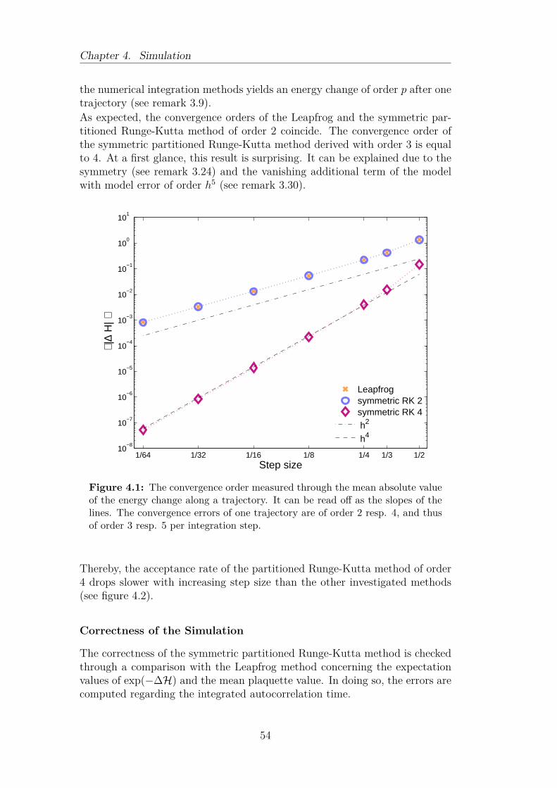
Chapter 4. Simulation
the numerical integration methods yields an energy change of order p after onetrajectory (see remark 3.9).As expected, the convergence orders of the Leapfrog and the symmetric par-titioned Runge-Kutta method of order 2 coincide. The convergence order ofthe symmetric partitioned Runge-Kutta method derived with order 3 is equalto 4. At a first glance, this result is surprising. It can be explained due to thesymmetry (see remark 3.24) and the vanishing additional term of the modelwith model error of order h5 (see remark 3.30).
1/64 1/32 1/16 1/8 1/4 1/3 1/210
−8
10−7
10−6
10−5
10−4
10−3
10−2
10−1
100
101
Step size
⟨ |∆
H| ⟩
Leapfrogsymmetric RK 2symmetric RK 4
h2
h4
Figure 4.1: The convergence order measured through the mean absolute valueof the energy change along a trajectory. It can be read off as the slopes of thelines. The convergence errors of one trajectory are of order 2 resp. 4, and thusof order 3 resp. 5 per integration step.
Thereby, the acceptance rate of the partitioned Runge-Kutta method of order4 drops slower with increasing step size than the other investigated methods(see figure 4.2).
Correctness of the Simulation
The correctness of the symmetric partitioned Runge-Kutta method is checkedthrough a comparison with the Leapfrog method concerning the expectationvalues of exp(−∆H) and the mean plaquette value. In doing so, the errors arecomputed regarding the integrated autocorrelation time.
54

4.3. Results
1/64 1/32 1/16 1/8 1/4 1/3 1/275
80
85
90
95
100
105
Step size
⟨ Acc
epat
nce
rate
[%] ⟩
Leapfrogsymmetric RK 2,symmetric RK 4,
Figure 4.2: Acceptance rate of the simulations after 5000 trajectories.
The reference value of the mean plaquette value of the model is known as⟨tr(U)⟩ = 0.8669(2) (personal communication with Prof. Dr. Knechtli). It ismet in the realized simulations as visualized in figure 4.3.
1/64 1/32 1/16 1/8 1/4 1/3 1/20.845
0.85
0.855
0.86
0.865
0.87
0.875
0.88
0.885
Step size
⟨ Pla
quet
te ⟩
Leapfrogsymmetric RK 2symmetric RK 4reference value
Figure 4.3: Expectation value of the mean plaquette value
The expectation value of exp(−∆H) serves as a measure for the volume-preservation. It has to be equal to one in the region of the errors. This isillustrated in figure 4.4. It can be seen that there may occur instabilities forlarger step sizes if methods of convergence order 2 are used. These instabilitiesvanish for the Runge-Kutta method of order 4.
55
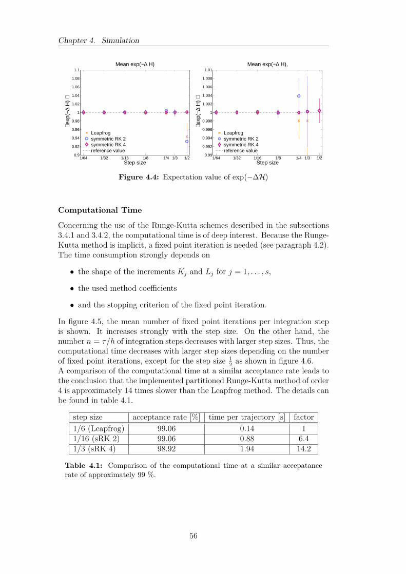
Chapter 4. Simulation
1/64 1/32 1/16 1/8 1/4 1/3 1/20.9
0.92
0.94
0.96
0.98
1
1.02
1.04
1.06
1.08
1.1
Step size
⟨ exp
(−∆
H)
⟩Mean exp(−∆ H)
Leapfrogsymmetric RK 2symmetric RK 4reference value
1/64 1/32 1/16 1/8 1/4 1/3 1/20.99
0.992
0.994
0.996
0.998
1
1.002
1.004
1.006
1.008
1.01
Step size
⟨ exp
(−∆
H)
⟩
Mean exp(−∆ H),
Leapfrogsymmetric RK 2symmetric RK 4reference value
Figure 4.4: Expectation value of exp(−∆H)
Computational Time
Concerning the use of the Runge-Kutta schemes described in the subsections3.4.1 and 3.4.2, the computational time is of deep interest. Because the Runge-Kutta method is implicit, a fixed point iteration is needed (see paragraph 4.2).The time consumption strongly depends on
• the shape of the increments Kj and Lj for j = 1, . . . , s,
• the used method coefficients
• and the stopping criterion of the fixed point iteration.
In figure 4.5, the mean number of fixed point iterations per integration stepis shown. It increases strongly with the step size. On the other hand, thenumber n = τ/h of integration steps decreases with larger step sizes. Thus, thecomputational time decreases with larger step sizes depending on the numberof fixed point iterations, except for the step size 1
2 as shown in figure 4.6.A comparison of the computational time at a similar acceptance rate leads tothe conclusion that the implemented partitioned Runge-Kutta method of order4 is approximately 14 times slower than the Leapfrog method. The details canbe found in table 4.1.
step size acceptance rate [%] time per trajectory [s] factor1/6 (Leapfrog) 99.06 0.14 11/16 (sRK 2) 99.06 0.88 6.41/3 (sRK 4) 98.92 1.94 14.2
Table 4.1: Comparison of the computational time at a similar accepatancerate of approximately 99 %.
56
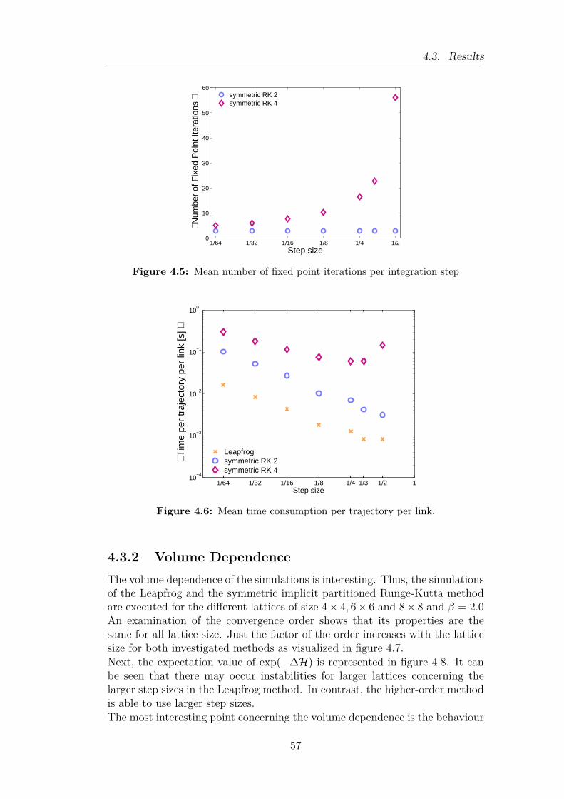
4.3. Results
1/64 1/32 1/16 1/8 1/4 1/20
10
20
30
40
50
60
Step size
⟨ Num
ber
of F
ixed
Poi
nt It
erat
ions
⟩
symmetric RK 2symmetric RK 4
Figure 4.5: Mean number of fixed point iterations per integration step
1/64 1/32 1/16 1/8 1/4 1/3 1/2 110
−4
10−3
10−2
10−1
100
Step size
⟨ Tim
e pe
r tr
ajec
tory
per
link
[s] ⟩
Leapfrogsymmetric RK 2symmetric RK 4
Figure 4.6: Mean time consumption per trajectory per link.
4.3.2 Volume DependenceThe volume dependence of the simulations is interesting. Thus, the simulationsof the Leapfrog and the symmetric implicit partitioned Runge-Kutta methodare executed for the different lattices of size 4× 4, 6× 6 and 8× 8 and β = 2.0An examination of the convergence order shows that its properties are thesame for all lattice size. Just the factor of the order increases with the latticesize for both investigated methods as visualized in figure 4.7.Next, the expectation value of exp(−∆H) is represented in figure 4.8. It canbe seen that there may occur instabilities for larger lattices concerning thelarger step sizes in the Leapfrog method. In contrast, the higher-order methodis able to use larger step sizes.The most interesting point concerning the volume dependence is the behaviour
57
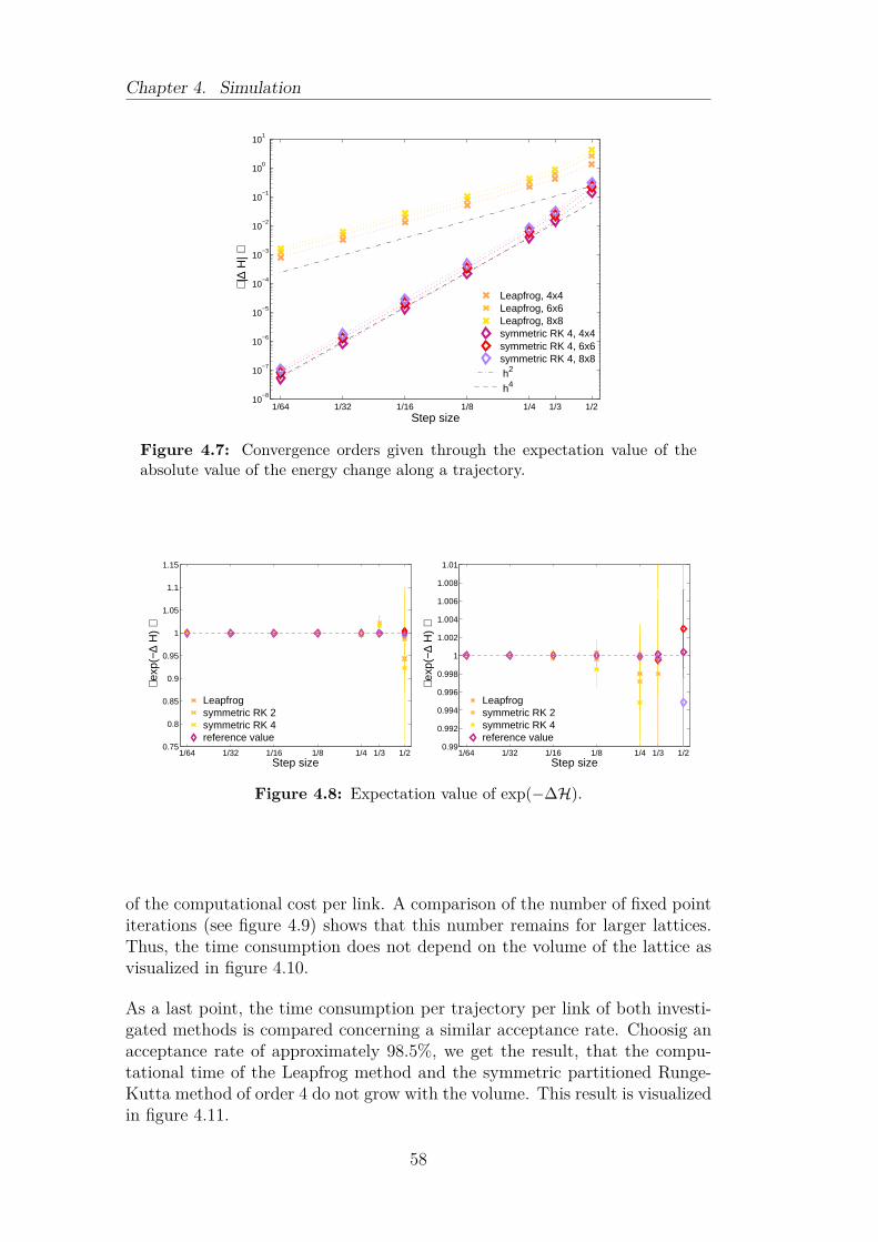
Chapter 4. Simulation
1/64 1/32 1/16 1/8 1/4 1/3 1/210
−8
10−7
10−6
10−5
10−4
10−3
10−2
10−1
100
101
Step size
⟨ |∆
H| ⟩
Leapfrog, 4x4Leapfrog, 6x6Leapfrog, 8x8symmetric RK 4, 4x4symmetric RK 4, 6x6symmetric RK 4, 8x8 h2
h4
Figure 4.7: Convergence orders given through the expectation value of theabsolute value of the energy change along a trajectory.
1/64 1/32 1/16 1/8 1/4 1/3 1/20.75
0.8
0.85
0.9
0.95
1
1.05
1.1
1.15
Step size
⟨ exp
(−∆
H)
⟩
Leapfrogsymmetric RK 2symmetric RK 4reference value
1/64 1/32 1/16 1/8 1/4 1/3 1/20.99
0.992
0.994
0.996
0.998
1
1.002
1.004
1.006
1.008
1.01
Step size
⟨ exp
(−∆
H)
⟩
Leapfrogsymmetric RK 2symmetric RK 4reference value
Figure 4.8: Expectation value of exp(−∆H).
of the computational cost per link. A comparison of the number of fixed pointiterations (see figure 4.9) shows that this number remains for larger lattices.Thus, the time consumption does not depend on the volume of the lattice asvisualized in figure 4.10.
As a last point, the time consumption per trajectory per link of both investi-gated methods is compared concerning a similar acceptance rate. Choosig anacceptance rate of approximately 98.5%, we get the result, that the compu-tational time of the Leapfrog method and the symmetric partitioned Runge-Kutta method of order 4 do not grow with the volume. This result is visualizedin figure 4.11.
58
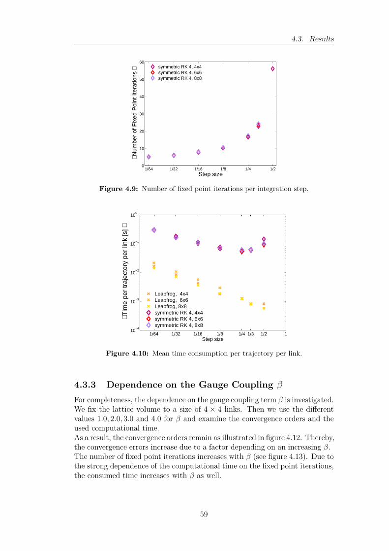
4.3. Results
1/64 1/32 1/16 1/8 1/4 1/20
10
20
30
40
50
60
Step size
⟨ Num
ber
of F
ixed
Poi
nt It
erat
ions
⟩
symmetric RK 4, 4x4symmetric RK 4, 6x6symmetric RK 4, 8x8
Figure 4.9: Number of fixed point iterations per integration step.
1/64 1/32 1/16 1/8 1/4 1/3 1/2 110
−4
10−3
10−2
10−1
100
Step size
⟨ Tim
e pe
r tr
ajec
tory
per
link
[s] ⟩
Leapfrog, 4x4Leapfrog, 6x6Leapfrog, 8x8symmetric RK 4, 4x4symmetric RK 4, 6x6symmetric RK 4, 8x8
Figure 4.10: Mean time consumption per trajectory per link.
4.3.3 Dependence on the Gauge Coupling β
For completeness, the dependence on the gauge coupling term β is investigated.We fix the lattice volume to a size of 4 × 4 links. Then we use the differentvalues 1.0, 2.0, 3.0 and 4.0 for β and examine the convergence orders and theused computational time.As a result, the convergence orders remain as illustrated in figure 4.12. Thereby,the convergence errors increase due to a factor depending on an increasing β.The number of fixed point iterations increases with β (see figure 4.13). Due tothe strong dependence of the computational time on the fixed point iterations,the consumed time increases with β as well.
59
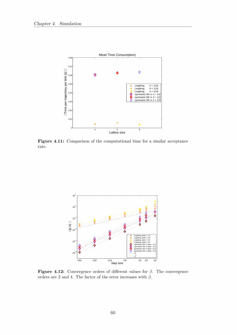
Chapter 4. Simulation
4 6 80
0.01
0.02
0.03
0.04
0.05
0.06
0.07
0.08
Lattice size
⟨ Tim
e pe
r tr
ajec
tory
per
link
[s] ⟩
Mean Time Consumption)
Leapfrog, h = 1/16Leapfrog, h = 1/16Leapfrog, h = 1/16symmetric RK 4, h = 1/3symmetric RK 4, h = 1/3symmetric RK 4, h = 1/3
Figure 4.11: Comparison of the computational time for a similar acceptancerate.
1/64 1/32 1/16 1/8 1/4 1/3 1/2
10−8
10−6
10−4
10−2
100
102
Step size
⟨ |∆
H| ⟩
Leapfrog, beta = 1.0Leapfrog, beta = 2.0Leapfrog, beta = 3.0Leapfrog, beta = 4.0symmetric RK 4, beta = 1.0symmetric RK 4, beta = 2.0symmetric RK 4, beta = 3.0symmetric RK 4, beta = 4.0
h2
h4
Figure 4.12: Convergence orders of different values for β. The convergenceorders are 2 and 4. The factor of the error increases with β.
60

4.3. Results
1/64 1/32 1/16 1/8 1/4 1/20
10
20
30
40
50
60
Step size
⟨ Num
ber
of F
ixed
Poi
nt It
erat
ions
⟩
symm RK 4, beta =1.0symm RK 4, beta =2.0symm RK 4, beta =3.0symm RK 4, beta =4.0
1/64 1/32 1/16 1/8 1/4 1/3 1/2 110
−4
10−3
10−2
10−1
100
Step size
⟨ Tim
e pe
r tr
ajec
tory
per
link
[s] ⟩
Leapfrog, beta =1.0Leapfrog, beta =2.0Leapfrog, beta =3.0Leapfrog, beta =4.0symm RK 4, beta =1.0symm RK 4, beta =2.0symm RK 4, beta =3.0symm RK 4, beta =4.0
Figure 4.13: Left: The number of fixed point iterations for different values ofβ. Right: The computational time increases with β.
61

Chapter 4. Simulation
62

Conclusion and Outlook
The main result of this work is the insight that implicit partitioned Runge-Kutta methods can be used during the simulations of gauge theories. It canbe mentioned, that symmetric implicit partitioned Runge-Kutta methods havean even convergence order provided that the model error is small enough. Dueto the fact that a convergence order of 4 is reached in the simulations, it hasbeen shown that a convergence order greater than 2 can in fact be attained.Furthermore, the investigated implicit partitioned Runge-Kutta method ofconvergence order 4 is stable, which allows to use larger step sizes. So far,the complexity of the integration scheme described in lemma 3.21 preventsthe method from being more efficient than the Leapfrog integration scheme.Though, it needs to be said, that the main objective of this thesis has beenthe investigation of the feasibility of higher-order integration schemes besidesthe Leapfrog and splitting methods. Thus, there has been no attempt in opti-mizing this method until now.
The symplecticity, i.e volume-preservation is not considered in this thesis. Al-though the expectation value of the energy chage along a trajectory exp(−∆H)serves as a measure for volume-preservation, it should be shown numericallyby means of the Jacobian of the field configurations.As a next step, the time consumption of the implicit partitioned Runge-Kuttamethod should be examined. The fixed point iteration depends on matrixcomputations so far. It can be improved, e.g using a base of Pauli matrices.With this ansatz, only the coefficients of the Pauli base would have to becomputed. Furthermore, the stopping criterion used in the fixed point iterationcan be considered as well as the method coefficients. Probably, the coefficientscan be chosen in a way that the expensive parts have to be evaluated less often.Another possibility to save computational time is the change of the increment
Lj = ig([
exp(Wj
)exp
(12Ω1
)U0]).
Because of the two matrix exponential functions, its evaluation is very costly.
Another idea is the exchange of the used mapping U(t) = exp(Ω(t)U0) given inequation (3.9) and its appropriate differential equation Ω(t) = exp−1
Ω (see equa-tion (3.3)) with another one, e.g. the Cayley map. In doing so, the exponentialfunction and the truncation of the derivative of the inverse exponential mapwould be replaced. Since the computation of the matrix exponential function
63

Chapter 4. Simulation
is time-consuming, this could be advantageous. Another point is that the Tay-lor series used to determine the convergence orders depend on the truncationof the model and have to be computed for each convergence order separately.The derivative of the inverse Cayley map is not truncated, such that higherconvergence orders can be derived from lower ones.As a general remark, it can be said that the implicit partitioned Runge-Kuttamethod does not depend on the size of its used matrices. Thus, the schemecan be applied for any differential equations with result in a Lie group.
64

Appendix A
Theory
Definition A.1 (Haar measure). For any compact group G the Haar measureis the unique measure dU on G which is
• normalized: ∫
Gf(U)dU = 1,
• invariant:∫
Gf(U)dU =
∫
Gf(V U)dU =
∫
Gf(UV )dU ∀V ∈ G.
Definition A.2 (Lie Algebra). A Lie algebra g is a vector space over a fieldF with composition
[ , ] : g× g −→ g, (x, y) 7−→ [x, y]
which is called Lie bracket or commutator and satisfies the following conditions:
L1 Antisymmetry[x, y] = −[y, x] ∀x, y ∈ g
L2 Bilinearity
[αx + βy, z] = α[x, z] + β[y, z][x, αy + βz] = α[x, y] + β[x, z]
∀x, y, z ∈ g and α, β ∈ F
L3 Jacobi identity[x, [y, z]
]+[y, [z, x]
]+[z, [x, y]
]= 0 ∀x, y, z ∈ g
Remark A.3. We will consider the general linear Lie algebra g with commu-tator
[A,B] = AB −BA ∀A,B ∈ g.
Definition A.4 (Lie Group). A Lie group G is a group which is also a differ-entiable manifold. The group operation is a differentiable mapping G×G→ G.
65
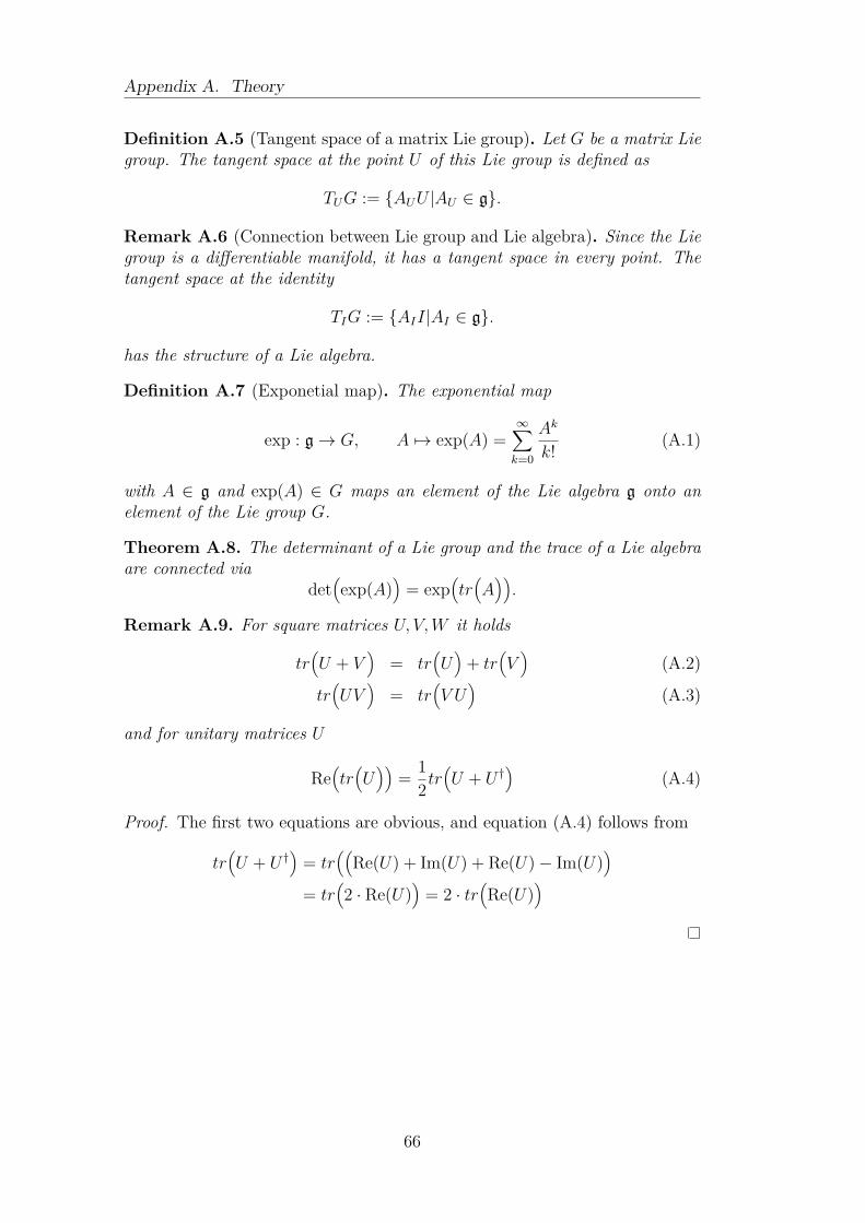
Appendix A. Theory
Definition A.5 (Tangent space of a matrix Lie group). Let G be a matrix Liegroup. The tangent space at the point U of this Lie group is defined as
TUG := AUU |AU ∈ g.
Remark A.6 (Connection between Lie group and Lie algebra). Since the Liegroup is a differentiable manifold, it has a tangent space in every point. Thetangent space at the identity
TIG := AII|AI ∈ g.
has the structure of a Lie algebra.
Definition A.7 (Exponetial map). The exponential map
exp : g → G, A 7→ exp(A) =∞∑
k=0
Ak
k! (A.1)
with A ∈ g and exp(A) ∈ G maps an element of the Lie algebra g onto anelement of the Lie group G.
Theorem A.8. The determinant of a Lie group and the trace of a Lie algebraare connected via
det(exp(A)
)= exp
(tr(A)).
Remark A.9. For square matrices U, V,W it holds
tr(U + V
)= tr
(U)
+ tr(V)
(A.2)
tr(UV
)= tr
(V U
)(A.3)
and for unitary matrices U
Re(tr(U))
= 12tr
(U + U †
)(A.4)
Proof. The first two equations are obvious, and equation (A.4) follows from
tr(U + U †
)= tr
((Re(U) + Im(U) + Re(U)− Im(U)
)
= tr(2 · Re(U)
)= 2 · tr
(Re(U)
)
66
Appendix B
Calculations
B.1 Check of the symmetry and the conver-gence order 2
Remark B.1. The coefficiens given in table 3.1 fulfill the symmetry conditions(3.12) and the order conditions (3.27)-(3.30) for convergence order 2.Proof. The order conditions will be checked with the coefficients from theButcher tableaus denoted in table 3.1:
(3.27) :s=2∑
j=1bj = b1 + b2 = 1
2 + 12 = 1
(3.28) :s=2∑
j=1bj = b1 + b2 = 1
2 + 12 = 1
(3.29) :s=2∑
j=1
(bj
s=2∑
k=1ajk)
= b1 · (a11a12) + b2 · (a21a22) = 12 ·
12 + 1
2 ·12 = 1
2
(3.30) :s=2∑
j=1
(bj
s=2∑
k=1ajk
)= b1 · (a11 + a12) + b2 · (a21 + a22) = 1
2 · 0 + 12 · 1 = 0 + 1
2 = 12
This means the partitioned Runge-Kutta method (3.26) with coefficients givenin table 3.1 fulfills convergence order two. Considering the symmetry condi-tions
b1 = 12 = b2
a1,1 = b2 − a22 = 12 − 0 = 1
2a1,2 = b2 − a21 = 1
2 −12 = 0
a2,1 = b1 − a12 = 12 − 0 = 1
2a2,2 = b1 − a11 = 1
2 −12 = 0
b1 = 12 = b2
a1,1 = b2 − a22 = 12 −
12 = 0
a1,2 = b2 − a21 = 12 −
12 = 0
a2,1 = b1 − a12 = 12 − 0 = 1
2a2,2 = b1 − a11 = 1
2 − 0 = 12
mentioned in the system of equations (3.12), the method is also symmetric.
67

Appendix B. Calculations
68

Bibliography
[1] J. C. Sexton and D. H. Weingarten. Hamiltonian evolution for the hybridMonte Carlo algorithm. Nucl. Phys., B380:665–678, 1992.
[2] C. Lubich E. Hairer and G. Wanner. Geometric Numerical Integration.Springer-Verlag Berlin Heidelberg, 2006.
[3] Christof Gattringer and Christian B. Lang. Quantum chromodynamics onthe lattice, an introductory presentation. Lecture notes in physics ; 788.Springer, 2010.
[4] Istvan Montvay and Gernot Munster. Quantum Fields on a Lattice. Cam-bridge University Press, 1994.
[5] Thomas DeGrand and Carleton DeTar. Lattice Methods for Quantum Chro-modynamics. World Scientific, 2006.
[6] B. J. Pendleton S. Duane, A. D. Kennedy and D. Roweth. Hybrid montecarlo. Physics Letters B, 195:216–222, 1987.
[7] Carsten Urbach. Untersuchung der Reversibilitatsverletzung beim Hybrid-Monthe-Carlo-Algorithmus. Master’s thesis, Freie Universitaet Berlin,2002.
69