Embed Size (px)
Citation preview

III-47
MOMENT FRAME MODEL
Grids 1 and 8 were modeled in conventional structural analysis software as two-dimensional models. The second-order option in the structural analysis program was not used. Rather, for illustration purposes, second-order effects are calculated separately, using the B1-B2 approximation method given in Specification Section C2.1b. The column and beam layouts for the moment frames follow. Although the frames on Grids A and F are the same, slightly heavier seismic loads accumulate on grid F, after accounting for the atrium area on Grid A and accidental torsion. The models are half-building models. The frame was originally modeled with W14×82 interior columns and W21×44 non-composite beams. This model had a drift that substantially exceeded the 0.025hsx story drift allowed per IBC Table 1617.3.1, Seismic Use Group I. The column size was incremented up to a W14×99 and the W21×44 beams were upsized to W24×55 (with minimum composite studs) and the beams were modeled with a stiffness of Ieq = Is. Alternatively, the beams could be modeled as = +0.6 0.4eq LB nI I I (Formula 24), s. This equation is given in AISC Design Guide 8. These changes resulted in a drift that satisfied the L / 400 limit. This layout is shown in the Grid A and F, Frame (½ building) layout that follows.
All of the vertical loads on the frame were modeled as point loads on the frame. As noted in the description of the dead load, W, in IBC Section 1617.5, 0.010 kip/ft2 is included in the dead load combinations. The remainder of the half-building model gravity loads were accumulated in the leaning column, which was connected to the frame portion of the model with pinned ended links. See Geschwindner, AISC Engineering Journal, Fourth Quarter 1994, A Practical Approach to the “Leaning” Column. The dead load and live load are shown in the load cases that follow. The wind and the seismic loads are modeled and distributed 1/14 to exterior columns and 1/7 to the interior columns. This approach minimizes the tendency to accumulate too much load in the lateral system nearest an externally applied load. There are four horizontal load cases. Two are the wind load and seismic load, per the previous discussion. In addition, notional loads of Ni = 0.002Yi were established. These load cases are shown in the load cases that follow. The same modeling procedures were used in the braced frame analysis. If column bases are not fixed in construction, they should not be fixed in the analysis.

III-48
The model layout, dead loads, live loads, wind loads, seismic loads, dead load notional loads, and live load notional loads for the moment frame are given as follows:

III-49

III-50

III-51

III-52

III-53
CALCULATION OF REQUIRED STRENGTH - THREE METHODS Three methods of determining the required strength including second-order effects are included below. A fourth method – second-order analysis by amplified first-order analysis – is found in Section C2.2b or the Specification. The method requires the inclusion of notional loads in the analysis, but all required strengths can be determined from a first-order analysis. For guidance on applying these methods, see the discussion in Manual Part 2 titled Required Strength, Effective Length, and Second-Order Effects. GENERAL INFORMATION FOR ALL THREE METHODS Seismic load dominates over winds loads in the moment frame direction of this example building. Although the frame analysis that follows was run for all LRFD and ASD load combinations, the column unity design check is highly dependent on the moment portion, and therefore, the controlling equations are those with the load combinations shown below. A typical column near the middle of the frame is analyzed, but the first interior columns and the end columns were also checked. Beam analysis is covered after the three different methods are shown for the typical interior column. Note: The second-order analysis and the unity checks are based on the moments and column loads for the particular load combination being checked, and not on the envelope of maximum values. METHOD 1. EFFECTIVE LENGTH METHOD This method accounts for second-order effects in frames by amplifying the axial forces and moments in members and connections from a first-order analysis.
A first-order frame analysis is run using the load combinations for LRFD or ASD. A minimum lateral load (notional load) equal to 0.2% of the gravity loads is included for any load case for which the lateral load is not already greater. The general load combinations are in ASCE 7 and are summarized in Part 2 of the Manual.
A summary of the axial loads, moments and 1st floor drifts from the first-order computer analysis is shown below:
Specification C2.2a
LRFD ASD 1.2D ± 1.0E + 0.5L + 0.2S
(Controls for columns and beams) For Interior Column Design: Pu = 335 kips M1u = 157 kip-ft (from first-order analysis) M2u = 229 kip-ft (from first-order analysis) First-order first floor drift = 0.562 in.
D ± (W or 0.7 E) (Controls for columns) D + 0.75(W or 0.7E) + 0.75L + 0.75(Lr or S or R) (Controls for beams) For Interior Column Design: Pa = 247 kips M1a = 110 kip-ft (from first-order analysis) M2a = 161 kip-ft (from first-order analysis) First-order first floor drift = 0.394 in.
The required second-order flexural strength, Mr, and axial strength, Pr, are as follows: For typical interior columns the gravity-load moments are approximately balanced, therefore, Mnt = 0.0 kip-ft
III-54
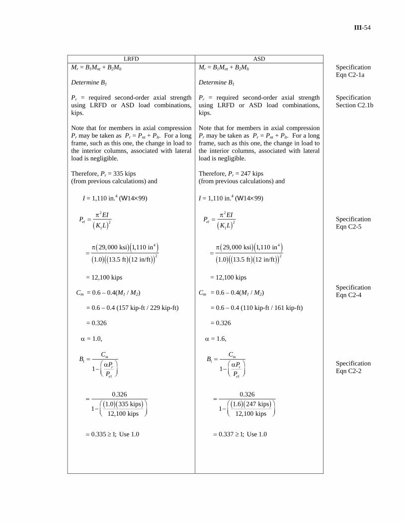
LRFD ASD Mr = B1Mnt + B2Mlt
Determine B1 Pr = required second-order axial strength using LRFD or ASD load combinations, kips. Note that for members in axial compression Pr may be taken as Pr = Pnt + Plt. For a long frame, such as this one, the change in load to the interior columns, associated with lateral load is negligible. Therefore, Pr = 335 kips (from previous calculations) and I = 1,110 in.4 (W14×99)
( )
( ) ( )( ) ( ) ( )( )
2
21
4
2
29,000 ksi 1,110 in
1.0 13.5 ft 12 in/ft
elEIP
K Lπ
=
π=
= 12,100 kips Cm = 0.6 – 0.4(M1 / M2) = 0.6 – 0.4 (157 kip-ft / 229 kip-ft) = 0.326 α = 1.0,
( ) ( )
1
1
1
0.326 1.0 335 kips
112,100 kips
0.335 1; Use 1.0
m
r
e
CB
PP
=⎛ ⎞α
− ⎜ ⎟⎝ ⎠
=⎛ ⎞
− ⎜ ⎟⎝ ⎠
= ≥
Mr = B1Mnt + B2Mlt
Determine B1 Pr = required second-order axial strength using LRFD or ASD load combinations, kips. Note that for members in axial compression Pr may be taken as Pr = Pnt + Plt. For a long frame, such as this one, the change in load to the interior columns, associated with lateral load is negligible. Therefore, Pr = 247 kips (from previous calculations) and I = 1,110 in.4 (W14×99)
( )
( ) ( )( ) ( ) ( )( )
2
21
4
2
29,000 ksi 1,110 in
1.0 13.5 ft 12 in/ft
elEIP
K Lπ
=
π=
= 12,100 kips Cm = 0.6 – 0.4(M1 / M2) = 0.6 – 0.4 (110 kip-ft / 161 kip-ft) = 0.326 α = 1.6,
( ) ( )
1
1
1
0.326 1.6 247 kips
112,100 kips
0.337 1; Use 1.0
m
r
e
CB
PP
=⎛ ⎞α
− ⎜ ⎟⎝ ⎠
=⎛ ⎞
− ⎜ ⎟⎝ ⎠
= ≥
Specification Eqn C2-1a Specification Section C2.1b Specification Eqn C2-5 Specification Eqn C2-4 Specification Eqn C2-2

III-55
Calculate B2
2
2
1
1=
⎛ ⎞α− ⎜ ⎟⎜ ⎟
⎝ ⎠
∑∑
nt
e
BP
P
where: α = 1.0,
5, 250 kips (from computer output)=∑ ntP and
2 may be taken as =
where is taken as 0.85 for moment frames
1.2 1.0 0.5 0.2
= 195 kips (Horizontal) (from previous seismic force distribution calculations)
e MH
M
HLP R
R
H D E L S
∆
= + + +
∑∑
∑
H = 0.562 in. (from computer output)∆
( ) ( ) ( )
2
195 kips 13.5 ft 12 in/ft 0.85
0.562 in.
47,800 kips
eP =
=
∑
( ) ( )
2
2
1
1
1 1.0 5, 250 kips
147,800 kips
1.12 1
=⎛ ⎞α
− ⎜ ⎟⎜ ⎟⎝ ⎠
=⎛ ⎞
− ⎜ ⎟⎝ ⎠
= ≥
∑∑
nt
e
BP
P
Calculate amplified moment
= (1.0)(0.0 kip-ft) + (1.12)(229 kip-ft) = 256 kip-ft
Calculate amplified axial load
Pr = 335 kips (from computer analysis)
Calculate B2
2
2
1
1=
⎛ ⎞α− ⎜ ⎟⎜ ⎟
⎝ ⎠
∑∑
nt
e
BP
P
where: α= 1.6,
3, 750 kips (from computer output)=∑ ntP and
2 may be taken as =
where is taken as 0.85 for moment frames
0.7
= 137 kips (Horizontal)(from previous seismic force distribution calculations)
e MH
M
HLP R
R
H D E
∆
= +
∑∑
∑
H = 0.394 in. (from computer output)∆
( ) ( ) ( )
2
137 kips 13.5 ft 12 in/ft 0.85
0.394 in.
47,900 kips
eP =
=
∑
( ) ( )
2
2
1
1
1 1.6 3,750 kips
147,900 kips
1.14 1
=⎛ ⎞α
− ⎜ ⎟⎜ ⎟⎝ ⎠
=⎛ ⎞
− ⎜ ⎟⎝ ⎠
= ≥
∑∑
nt
e
BP
P
Calculate amplified moment
= (1.0)(0.0 kip-ft) + (1.14)(161 kip-ft) = 184 kip-ft Calculate amplified axial load Pr = 247 kips (from computer analysis)
Specification Section C2.1b Specification Eqn C2-6b Specification Eqn C2-3

III-56
Pr = Pnt + B2Plt = 335 kips + (1.12)(0.0 kips) = 335 kips
Determine the controlling effective length For out-of-plane buckling in the braced frame Ky=1.0 For in-plane buckling in the moment frame, use the nomograph
Kx=1.43
To account for leaning columns in the controlling load case For leaning columns,
3010 kips
2490 kips
Q
P
=
=
∑∑
= +
= + =
= =
∑∑
1
3010 1.43 1 2.132490
2.13(13.5) 17.3/ 1.66
o
x
x y
QK K
P
KLr r
Pr = Pnt + B2Plt = 247 kips + (1.14)(0.0 kips) = 247 kips
Determine the controlling effective length For out-of-plane buckling in the braced frame Ky=1.0 For in-plane buckling in the moment frame, use the nomograph
Kx=1.43
To account for leaning columns in the controlling load case For leaning columns,
2140 kips
1740 kips
Q
P
=
=
∑∑
= +
= + =
= =
∑∑
1
2140 1.43 1 2.141740
2.14(13.5) 17.4/ 1.66
o
x
x y
QK K
P
KLr r
Commentary Section C2.2b

III-57
1,041 kips ( 14 99 @ = 17.3 ft)
335 kips 0.321 0.21,041 kips
646 kip-ft ( 14 99)
89
8 256 kip-ft0.3219 646 kip-ft
0.673 1.0
c
r
c
cx
ryrxr
c cx cy
P KL
PP
M
MMPP M M
= ×
= = ≥
= ×
⎛ ⎞⎛ ⎞+ +⎜ ⎟ ⎜ ⎟⎝ ⎠ ⎝ ⎠
⎛ ⎞⎛ ⎞= + ⎜ ⎟ ⎜ ⎟⎝ ⎠ ⎝ ⎠
= ≤
W
W
o.k.
692 kips ( 14 99 @ = 17.4 ft)
247 kips 0.357 0.2692 kips
430 kip-ft ( 14 99)
89
8 184 kip-ft0.3579 430 kip-ft
0.737 1.0
c
r
c
cx
ryrxr
c cx cy
P KL
PP
M
MMPP M M
= ×
= = ≥
= ×
⎛ ⎞⎛ ⎞+ +⎜ ⎟ ⎜ ⎟⎝ ⎠ ⎝ ⎠
⎛ ⎞⎛ ⎞= + ⎜ ⎟ ⎜ ⎟⎝ ⎠ ⎝ ⎠
= ≤
W
W
o.k.
Specification Sect H1.1 Manual Table 4-1 Manual Table 3-2 Specification Eqn H1-1a

III-58
METHOD 2. SIMPLIFIED DETERMINATION OF REQUIRED STRENGTH A method of second-order analysis based upon drift limits and other assumptions is described in Chapter 2 of the Manual. A first-order frame analysis is run using the load combinations for LRFD or ASD. A minimum lateral load (notional load) equal to 0.2% of the gravity loads is included for any load case for which the lateral load is not already greater.
LRFD ASD 1.2D ± 1.0E + 0.5L + 0.2S (Controls
columns and beams) For a first-order analysis For Interior Column Design: Pu = 335 kips M1u = 157 kip-ft (from first-order analysis) M2u = 229 kip-ft (from first-order analysis) First-floor first-order drift = 0.562 in.
D ± (W or 0.7 E) (Controls columns) D + 0.75(W or 0.7E) + 0.75L + 0.75(Lr or S or R) (Controls beams) For a first-order analysis For Interior Column Design: Pa = 247 kips M1a = 110 kip-ft (from first-order analysis) M2a = 161 kip-ft (from first-order analysis) First-floor first-order drift = 0.394 in.
Then the following steps are executed.
LRFD ASD Step 1:
Lateral load = 195 kips Deflection due to first-order elastic analysis ∆ = 0.562 in. between first and second floor Floor height = 13.5 ft Drift ratio = (13.5 ft)(12 in/ft) / 0.562 in = 288 Step 2: Design story drift limit = 0.025 hxs = h/400 Adjusted Lateral load = (288/ 400)(195 kips) = 141 kips
Step 1: Lateral load = 140 kips Deflection due to first-order elastic analysis ∆ = 0.394 in. between first and second floor Floor height = 13.5 ft Drift ratio = (13.5 ft)(12 in/ft) / 0.394 in = 411 Step 2: Design story drift limit = 0.025 hxs = h/400 Adjusted Lateral load = (411 / 400)(137 kips) = 141 kips
IBC Table 1617.3.1

III-59
Step 3:
( )
( )
total story loadLoad ratio = 1.0lateral load
5, 250 kips = 1.0141 kips
= 37.2
Interpolating from the table: B2 = 1.1 Which matches the value obtained in the first method to the 2 significant figures of the table
Step 3: (for an ASD design the ratio must be factored by 1.6)
( )
( )
total story loadLoad ratio = 1.6lateral load
3,750 kips = 1.6141 kips
= 42.6
Interpolating from the table: B2 = 1.1 Which matches the value obtained in the first method to the 2 significant figures of the table
Manual Page 2-12
Note: Because the table is intentionally based on two significant figures, this value is taken as 1.1 rather than an interpolated value > 1.1. This convenient selection is within the accuracy of the method. Since the selection is in the shaded area of the chart, K=1.0.
Step 4. Multiply all the forces and moment from the first-order analysis by the value obtained from the table.
LRFD ASD Mr = B2(Mnt + Mlt)
= 1.1(0 kip-ft + 229 kip-ft) = 252 kip-ft Pr = 1.1(Pnt + Plt) = 1.1(335 kips +0.0 kips) = 368 kips
368 kips For 0.323 0.21,140 kips
where1,140 kips ( 14 99 @ =13.5 ft)
646 kip-ft ( 14 99)
89
8 252 kip-ft0.3239 646 kip-ft
0.670 1.0
r
c
c
cx
ryrxr
c cx cy
PP
P KL
M
MMPP M M
= = ≥
= ×
= ×
⎛ ⎞⎛ ⎞+ +⎜ ⎟⎜ ⎟⎝ ⎠ ⎝ ⎠
⎛ ⎞⎛ ⎞= + ⎜ ⎟ ⎜ ⎟⎝ ⎠ ⎝ ⎠
= ≤
W
W
o.k.
Mr = B2(Mnt + Mlt) = 1.1(0 kip-ft + 161 kip-ft) = 177 kip-ft Pr = 1.1(Pnt + Plt) = 1.1(247 kips +0.0 kips) = 272 kips
272 kips For 0.358 0.2759 kips
759 kips ( 14 99 @ = 13.5 ft)
430 kip-ft ( 14 99)
89
8 177 kip-ft0.3589 430 kip-ft
0.724 1.0
r
c
c
cx
ryrxr
c cx cy
PP
P KL
M
MMPP M M
= = ≥
= ×
= ×
⎛ ⎞⎛ ⎞+ +⎜ ⎟⎜ ⎟⎝ ⎠ ⎝ ⎠
⎛ ⎞⎛ ⎞= + ⎜ ⎟ ⎜ ⎟⎝ ⎠ ⎝ ⎠
= ≤
W
W
o.k.
Specification Sect H1.1 Manual Table 4-1 Manual Table 3-2 Specification Eqn H1-1a

III-60
METHOD 3. DIRECT ANALYSIS METHOD Second-order analysis by the direct analysis method is found in Appendix 7 of the Specification. This method requires that both the flexural stiffness and axial stiffness be reduced and that 0.2% notional lateral loads be applied in the analysis. The combination of these two modifications account for the second-order effects and the results for design can be taken directly from the analysis. A summary of the axial loads, moments and 1st floor drifts from first-order analysis is shown below:
LRFD ASD 1.2D ± 1.0E + 0.5L + 0.2S (Controls
columns and beams) For a 1st order analysis with notional loads and reduced stiffness: For Interior Column Design: Pu = 335 kips M1u = 157 kip-ft (from first-order analysis) M2u = 229 kip-ft (from first-order analysis) First-floor drift due to reduced stiffnesses = 0.703 in.
D ± (W or 0.7 E) (Controls columns) D + 0.75(W or 0.7E) + 0.75L + 0.75(Lr or S or R) (Controls beams) For a 1st order analysis with notional loads and with reduced stiffness: For Interior Column Design: Pa = 247 kips M1a = 110 kip-ft M2a = 161 kip-ft First-floor drift due to reduced stiffnesses = 0.493 in.
Note: For ASD, this method requires multiplying the ASD load combinations by a factor of 1.6 in analyzing the drift of the structure, and then dividing the results by 1.6 to obtain the required strengths. The ASD forces shown above include the multiplier of 1.6.
LRFD ASD For this method, =1.0.
1,140 kips ( 14 99 @ = 13.5 ft)
335 kips 0.294 0.21,140 kips
646 kip-ft ( 14 99)
c
r
c
cx
K
P KL
PP
M
= ×
= = ≥
= ×
W
W
Mr = B1Mnt + B2Mlt
Determine B1 Pr = required second-order axial strength using LRFD or ASD load combinations, kips. Note that for members in axial compression Pr may be taken as Pr = Pnt + Plt. For a long frame, such as this one, the change in load to the interior columns, associated with lateral load is negligible. Therefore, Pr = 335 kips (from previous calculations) and
For this method, =1.0
759 kips ( 14 99 @ = 13.5 ft)
247 kips 0.325 0.2759 kips
430 kip-ft ( 14 99)
c
r
c
cx
K
P KL
PP
M
= ×
= = ≥
= ×
W
W
Mr = B1Mnt + B2Mlt
Determine B1 Pr = required second-order axial strength using LRFD or ASD load combinations, kips. Note that for members in axial compression Pr may be taken as Pr = Pnt + Plt. For a long frame, such as this one, the change in load to the interior columns, associated with lateral load is negligible. Therefore, Pr = 247 kips (from previous calculations) and
Manual Table 4-1 Specification Sect H1.1 Manual Table 3-2
III-61
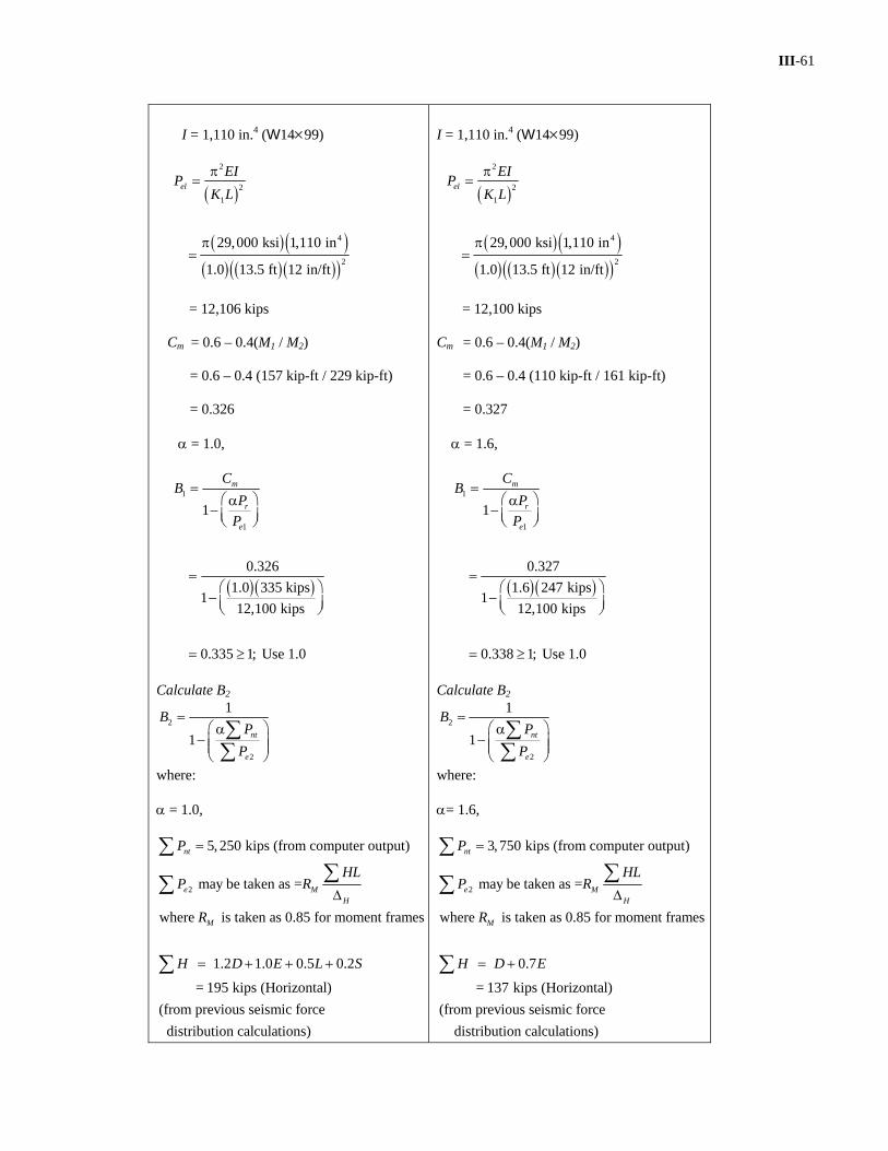
I = 1,110 in.4 (W14×99)
( )
( ) ( )( ) ( ) ( )( )
2
21
4
2
29,000 ksi 1,110 in
1.0 13.5 ft 12 in/ft
elEIP
K Lπ
=
π=
= 12,106 kips Cm = 0.6 – 0.4(M1 / M2) = 0.6 – 0.4 (157 kip-ft / 229 kip-ft) = 0.326 α = 1.0,
( ) ( )
1
1
1
0.326 1.0 335 kips
112,100 kips
0.335 1; Use 1.0
m
r
e
CB
PP
=⎛ ⎞α
− ⎜ ⎟⎝ ⎠
=⎛ ⎞
− ⎜ ⎟⎝ ⎠
= ≥
Calculate B2
2
2
1
1=
⎛ ⎞α− ⎜ ⎟⎜ ⎟
⎝ ⎠
∑∑
nt
e
BP
P
where: α = 1.0,
5, 250 kips (from computer output)=∑ ntP
2 may be taken as =
where is taken as 0.85 for moment frames
1.2 1.0 0.5 0.2
= 195 kips (Horizontal) (from previous seismic force distribution calculations)
e MH
M
HLP R
R
H D E L S
∆
= + + +
∑∑
∑
I = 1,110 in.4 (W14×99)
( )
( ) ( )( ) ( ) ( )( )
2
21
4
2
29,000 ksi 1,110 in
1.0 13.5 ft 12 in/ft
elEIP
K Lπ
=
π=
= 12,100 kips Cm = 0.6 – 0.4(M1 / M2) = 0.6 – 0.4 (110 kip-ft / 161 kip-ft) = 0.327 α = 1.6,
( ) ( )
1
1
1
0.327 1.6 247 kips
112,100 kips
0.338 1; Use 1.0
m
r
e
CB
PP
=⎛ ⎞α
− ⎜ ⎟⎝ ⎠
=⎛ ⎞
− ⎜ ⎟⎝ ⎠
= ≥
Calculate B2
2
2
1
1=
⎛ ⎞α− ⎜ ⎟⎜ ⎟
⎝ ⎠
∑∑
nt
e
BP
P
where: α= 1.6,
3, 750 kips (from computer output)=∑ ntP
2 may be taken as =
where is taken as 0.85 for moment frames
0.7
= 137 kips (Horizontal)(from previous seismic force distribution calculations)
e MH
M
HLP R
R
H D E
∆
= +
∑∑
∑

III-62
H = 0.703 in. ∆
( ) ( ) ( )2
195 kips 13.5 ft 12 in/ft 0.85
0.703 in.
38,200 kips
eP =
=
∑
( ) ( )
2
2
1
1
1 1.0 5,250 kips
138,200 kips
1.16 1
nt
e
BP
P
=⎛ ⎞α
− ⎜ ⎟⎝ ⎠
=⎛ ⎞
− ⎜ ⎟⎝ ⎠
= ≥
∑∑
Calculate amplified moment
= (1.0)(0.0 kip-ft) + (1.16)(229 kip-ft) = 266 kip-ft
Calculate amplified axial load
Pr = 335 kips (from computer analysis)
Pr = Pnt + B2Plt = 335 kips + (1.16)(0.0 kips) = 335 kips
89
8 266 kip-ft0.2949 646 kip-ft
0.660 1.0
ryrxr
c cx cy
MMPP M M
⎛ ⎞⎛ ⎞+ +⎜ ⎟ ⎜ ⎟⎝ ⎠ ⎝ ⎠
⎛ ⎞⎛ ⎞= + ⎜ ⎟ ⎜ ⎟⎝ ⎠ ⎝ ⎠
= ≤
H = 0.493 in. (from computer output)∆
( ) ( ) ( )2
137 kips 13.5 ft 12 in/ft 0.85
0.493 in.
38,300 kips
eP =
=
∑
( ) ( )
2
2
1
1
1 1.6 3,750 kips
138,300 kips
1.19 1
nt
e
BP
P
=⎛ ⎞α
− ⎜ ⎟⎝ ⎠
=⎛ ⎞
− ⎜ ⎟⎝ ⎠
= ≥
∑∑
Calculate amplified moment
= (1.0)(0.0 kip-ft) + (1.19)(161 kip-ft) = 192 kip-ft
Calculate amplified axial load Pr = 247 kips (from computer analysis) Pr = Pnt + B2Plt = 247 kips + (1.19)(0.0 kips) = 247 kips
89
8 192 kip-ft0.3259 430 kip-ft
0.722 1.0
ryrxr
c cx cy
MMPP M M
⎛ ⎞⎛ ⎞+ +⎜ ⎟ ⎜ ⎟⎝ ⎠ ⎝ ⎠
⎛ ⎞⎛ ⎞= + ⎜ ⎟ ⎜ ⎟⎝ ⎠ ⎝ ⎠
= ≤
Specification Eqn H1-1b

III-64
BRACED FRAME ANALYSIS
The braced frames at Grids 1 and 8 were analyzed for their lateral loads. The same stability design requirements from Chapter C were applied to this system.
Second-order analysis by amplified first-order analysis
The following is a method to account for second-order effects in frames by amplifying the axial forces and moments in members and connections from a first-order analysis.
First a first-order frame analysis is run using the load combinations for LRFD and ASD. From this analysis the critical axial loads, moments, and deflections are obtained.
The required second-order flexural strength, Mr, and axial strength, Pr, are as follows:
Specification C2.1b
LRFD ASD
( )
( ) ( )( ) ( ) ( )( )
2
21
4
2
4
29,000 ksi 425 in
1.0 13.5 ft 12 in/ft
= 4,635 kips
425 in ( 12 58)
elEIP
K L
I
π=
π=
= ×W
( ) ( )
2
2
1
1
1 1.0 5, 452 kips
1150,722 kips
1.04 1
5,452 kips (from computer output)
nt
e
nt
BP
P
P
=⎛ ⎞α
− ⎜ ⎟⎜ ⎟⎝ ⎠
=⎛ ⎞
− ⎜ ⎟⎝ ⎠
= ≥
=
∑∑
∑
( ) ( ) ( )
2
195 kips 13.5 ft 12 in/ft 1.0
0..210 in.
= 150,722 kips
e MH
HLP R=
∆
=
∑∑
( )
( ) ( )( ) ( ) ( )( )
2
21
4
2
4
29,000 ksi 425 in
1.0 13.5 ft 12 in/ft
= 4,635 kips
425 in ( 12 58)
elEIP
K L
I
π=
π=
= ×W
( )( )
2
2
1
1
1 1.6 3,894 kips
1150,722 kips
1.04 1
3,894 kips (from computer output)
nt
e
nt
BP
P
P
=⎛ ⎞α
− ⎜ ⎟⎜ ⎟⎝ ⎠
=⎛ ⎞
− ⎜ ⎟⎝ ⎠
= ≥
=
∑∑
∑
( ) ( ) ( )
2
137 kips 13.5 ft 12 in/ft = 1.0
0.147 in.
= 150,722 kips
e MH
HLP R=
∆∑∑
Specification Eqn C2-5 Specification Eqn C2-3 Specification Eqn C2-6b

III-65
H
1.2 1.0 0.2
= 195 kips (from previous calculations)
= 0.210 in. (from computer output)
H D E L S= + + +
∆
∑
Pr = Pnt + B2Plt = 242 kips + (1.04)(220 kips) = 470 kips
553 kips ( 12 58)
470 kips For 0.850 1.0553 kips
c
r
c
P
PP
= ×
= = ≤
W
H
0.7
137 kips (from previous calculations)
= 0.147 in. (from computer output)
H D E= +
=
∆
∑
Pr = Pnt + B2Plt = 173 kips + (1.04)(179 kips) = 360 kips
368 kips ( 12 58)
360 kipsFor 0.977 1.0368 kips
c
r
c
P
PP
= ×
= = ≤
W
Specification Eqn C2-1b Manual Table 4-1
Note: Notice that the lower displacements of the braced frame produce much lower values for B2. Similar values could be expected for the other two methods of analysis.