Embed Size (px)
Citation preview
CIVIL ENGINEERING STUDIES Structural Research Series No. 636
UILU-ENG-2004-2010
ISSN:0069-4274
REDUNDANCY IN STEEL MOMENT FRAME SYSTEMS UNDER SEISMIC EXCITATIONS
By
Kuo-Wei Liao Yi-Kwei Wen
DEPARTMENT OF CIVIL AND ENVIRONMENTAL ENGINEERING UNIVERSITY OF ILLINOIS AT URBANA-CHAMPAIGN URBANA, ILLINOIS
August 2004

iii
ABSTRACT
REDUNDANCY IN STEEL MOMENT FRAME SYSTEMS
UNDER SEISMIC EXCITATIONS
Kuo-Wei Liao, Ph.D. Candidate Department of Civil Engineering
University of illinois at Urbana-Champaign, 2004 Yi-Kwei Wen, Advisor
Although the importance and the positive effects of structural redundancy have
been long recognized, structural redundancy became the focus of research only after the
1994 Northridge and 1995 Kobe earthquakes. Several researchers have investigated the
benefit of redundancy to structural system. However, the definition and interpretation of
structural redundancy vary significantly and it remains a controversial subject.
A reliability/redundancy factor, p, was introduced in NEHRP 97, UBC 1997, and
IBC 2000. It is used as a multiplier of the lateral design earthquake load and takes into
account only the floor area and maximum element-story shear ratio. It lacks an adequate
rationale and can lead to poor structural designs (e.g. Searer G. R. and Freeman S. A.,
2002, Wen and Song, 2003). A new reliability/redundancy factor, primary a function of
plan configuration of the structures such as the number of moment frames in the direction
of earthquake excitations, has been adopted in NEHRP 2003 and also proposed in ASCE-
7. This new factor attempts a more reasonable and mechanism-based approach, and it is
likely to be implemented in other codes in the near future. However, the uniform
multiplied factor (1.3) of lateral design force for non-redundancy structures fails to
account for different structural configurations and could lead to serious damage in a
poorly designed structure. In view of the complicated nonlinear structural behaviors and
the effects of uncertainty in demand and capacity, redundancies of structures under
seismic loads can be measured meaningfully only in terms of reliability of a given system.
Therefore, a systematic and probabilistic study of redundancy in structural system is
needed and a uniform-risk redundancy factor is used for reliability assessment of
structural redundancy.
iv
To accurately describe the inelastic connection behaviors, the Bouc-W en model is
used and incorporated into the ABAQUS computer program. A 3-D finite element model
is developed, which allows one to examine the effects of 3-D motions including torsion
oscillation and biaxial bending interaction. The capacity uncertainties of connections that
were documented in the FEMAISAC projects are included in the Bouc-Wen model and
used in the reliability analysis.
Finally, a framework is proposed for evaluation of structural redundancy against·
incipient collapse limit state. In this framework: (1) the maximum column drift ratio
(MCDR) or biaxial spectral acceleration (BSA) is used to measure both demand and
capacity of a given building; (2) the demand and capacity analyses of a building are
performed, from which the probabilistic demand curves and the distribution of capacity
are constructed. The demand of a building is determined by conducting a series of time
history analyses under a given probability level. The capacity of a building against
incipient collapse is determined by performing the Incremental Dynamic Analyses (IDA);
(3) both aleatory and epistemic uncertainties in demand and capacity are taken into
account; (4) based on the results of (2), a uniform-risk redundancy factor, RR' for design
to achieve a uniform reliability level for buildings of different redundancies is obtained.
This method is also used to evaluate the redundancy of a given structural system. The p
factors in NEHRP 97 and in NEHRP 2003 and the proposed RR factor are compared and
the inadequacies of p factors are pointed out.

vi
ACKNOWLEDGEMENTS
The author wishes to express his sincere gratitude to Professor Yi-Kwei Wen for
his enthusiastic advice and guidance throughout the period of his study.
He is also grateful to the members of his committee, Professors Douglas A. Foutch,
James M. LaFave, and Youssef Hashash, for their precious and constructive
recommendations in his research.
The author would like to express the thanks for the softball team of Formosa. Their
friendships provide him a very strong support in his research.
The author appreciated the friendship from his colleagues and friends in the
Department of Civil and Environmental Engineering, especially from Ping Gu, Zhong
Zhuo Li and Svrakic Neda who shared with his study.
The author is especially indebted to his wife, Jung-Hsuan, for her patient and
constant love.
The support from the National Science Foundation under grants NSF-CMS 02-
18703 and EEC-9701785 to Mid-America Earthquake Center is gratefully acknowledged.

Vll
TABLE OF CONTENTS
LIST OFTABLES ..................................................................................... x
LIST OF FIGURES ................................................................................. xiii
CHAPTER 1 IN"TRODUCTION ..................................................................... 1
1.1 Background .................................................................................................................. 1
1.2 Previous Research on Structural Redundancy ............................................................ 3
1.3 Objective and Scope ..................................................................................................... 4
1.4 Organization ................................................................................................................. 6
CHAPTER 2 MODELING OF BEAM-COLUMN CONNECTIONS ......................... 9
2.1 Introduction .................................................................................................................. 9
2.2 Bouc-Wen Smooth Hysteresis Model ....................................................................... 10
2.3 Development of an ABAQUS User-Defined-Element ............................................. 12
2.3.1 Formulation of an ABAQUS Element ............................................................. 13
2.3.2 Modeling of Pre-Northridge and Post-Northridge Connections ..................... 14
2.3.3 Comparison with Experimental Result ............................................................ 16
2.4 Figures ........................................................................................................................ 17
CHAPTER 3 MODELING AND DESIGN OF BUILDINGS ................................. 23
3.1 Introduction ................................................................................................................ 23
3.2 Dynamic Time History Analysis Procedure .............................................................. 24
3.3 Modeling of Gravity Frames ...................................................................................... 25
3.4 Modeling of Ductile Partially Restrained Connections ............................................ 25
3.5 Modeling of Panel Zone ............................................................................................. 26
3.6 Modeling of Nonlinearity .......................................................................................... 28
viii
3.7 Modeling of Uncertainty ............................................................................................ 28
3.7.1 Modeling of Ground Motions ........................................................................... 29
3.7.2 Monte-Carlo Simulation in Materials and Member Properties ....................... 30
3.7.3 Incremental Dynamic Analysis ........................................................................ 30
3.7.4 Uncertainty Correction Factor for Modeling Errors ........................................ 31
3.8 Building Design .......................................................................................................... 32
3.8.1 Design Assumptions ......................................................................................... 32
3.8.2 Design Results ................................................................................................... 33
3.9 Tables ........................................................................................................................ 36
3.10 Figures ...................................................................................................................... 40
CHAPTER 4 STRUTURAL RESPONSE, DEMAND AND CAPACITY ANAL YSES ... 47
4.1 Introduction ................................................................................................................ 47
4.2 Responses Analyses of 3- and 12-Story Buildings ................................................... 47
4.2.1 Free Vibration Analyses ................................................................................... 48
4.2.2 Dynamic Time History Analyses ..................................................................... 50
4.3 Effects of Panel Zone ................................................................................................. 51
4.4 Comparisons of pre-Northridge and post-Northridge Connections ......................... 52
4.5 Effects of Connection Fracture .................................................................................. 53
4.6 Effects of Elastic-Plastic Column of Moment Frame ............................................... 54
4.7 Effects of Post-Fracture Behavior of Connections on MCDR Demand .................. 55
4.8 Performance Evaluation of 3-story Buildings ........................................................... 56
4.8.1 Demand Analyses ............................................................................................. 57
4.8.2 Structural Capacity by Incremental Dynamic Analysis ................................... 57
4.9 Performance Evaluation of 12-story Buildings ......................................................... 59
4.9.1 Demand Analyses ............................................................................................. 59
4.9.2 Structural Capacity by Incremental Dynamic Analyses .................................. 59
4.10 Response of Buildings of Equal Floor Aspect Ratios ............................................. 60
4.11 Tables ........................................................................................................................ 61
ix
4.12 Figures ...................................................................................................................... 70
<:~Ft 5 ~~IJ\J3~I1L1{ ~ ~I)1J]\f.[)~c:1{ ........................................ 107
5.1 Introduction .............................................................................................................. 107
5.2 The Fteliability/Redundancy Factor in NEHRP 97 ................................................. 108
5.3 The NEHRP Proposal2-1Ft (NEHRP 2003) ........................................................... 110
5.4 Uniform-rusk Ftedundancy Factor ........................................................................... 111
5.4.1 Methods of I)eterrnining the Uniform-rusk Ftedundancy Factor .................. 112
5.4.2 C:omparison of Ftesults of 3-Story Buildings ................................................. 113
5.4.3 C:omparison of Ftesults of 12-Story Buildings ............................................... 114
5.4.4 Ftedundancy as Function of Floor Area .......................................................... 115
5.5 Ftegression Analysis of the Uniform-rusk Ftedundancy Factors ............................ 116
5.6 Investigation of the Seismic Intensity Measures ..................................................... 117
5.7 Fragility Analyses and the Limit State Probability Analyses ................................. 119
5.8 Tables ........................................................................................................................ 121
5.9 Figures ...................................................................................................................... 129
<:HAPTEFt 6 <:ONc:~USION ~ RE<:OMMENI)ATIONS .............................. 136
6.1 C:onclusions .............................................................................................................. 136
6.2 Recommendations for Future Ftesearch ................................................................... 140
APPENDIX A S1{STEM ~I)1J]\f.[)~C:1{ OF SIMP~E PARALLEL SYSTEMS ...... 142
APPENDIX B STATISTI<:AL TEST ~ ~SIDUAL DIAGNOSIS ................... 146
~FE~NC:ES ..................................................................................................................... 148
VITA ..................................................................................................................................... 153

x
LIST OF TABLES
Table 3.1 Design Details of Moment Frames of 3-Story Buildings .................................. 36
Table 3.2 Design Details of Moment Frames of 12-Story Buildings ................................ 37
Table 3.3 Design Details of Gravity Frames of 3-Story Building ..................................... 38
Table 3.4 Design Details of Gravity Frames of 12-Story Building ................................... 38
Table 3.5 Periods of 3-story and 12-Story Buildings (Second) ......................................... 39
Table 3.6 Dimensions and Properties of Plate Girders. (Base Unit: inch) ........................ 39
Table 4.1 Statistics of MCDR Demand on 3-Story Buildings at Two Hazard Levels ..... 61
Table 4.2 Statistics of Drift Capacity against Incipient Collapse of pre-Northridge and
post-Northridge Buildings .................................................................................. 61
Table 4.3 Statistics of MCDR Demand on Buildings with Different post-to-pre Fracture
Moment Capacity Ratios at Two Hazard Levels ............................................... 62
Table 4.4 Relationship of Rotational Capacity and the Depth of Beams .......................... 62
Table 4.5 Statistics of MCDR Demand on Each Building at Two Hazard Levels (3-Story
Buildings) ............................................................................................................ 63
Table 4.6 Statistics of BSA of Each Building (3-Story Buildings) ................................... 63
Table 4.7 Statistics of Capacities (MCDR) of Each Building (3-Story Buildings) .......... 64
Table 4.8 Structural Demand (MCDR) for 3bay _3bay Building with Three Different
Modeling ............................................................................................................. 64
Table 4.9 Statistics of Capacities of 3bay _3bay Building with Different Modeling (3-
Story) ................................................................................................................... 65
Table 4.10 Comparison of System Capacity (MCDR) for 2D Building with Different
Modelings-( 1) ..................................................................................................... 65
Table 4.11 Comparison of System Capacity (MCDR) for 2D Building with Different
Modelings-(2) ..................................................................................................... 66
Table 4.12 Statistics of MCDR Demand on Each Building at Two Hazard Levels (12-
Story Buildings) .................................................................................................. 66

xi
Table 4.13 Statistics of BSA of Each Building (l2-Story Buildings) at Two Probability
Levels .................................................................................................................. 67
Table 4.14 Statistics of Capacities (MCDR) of Each Building (l2-Story Buildings) ........ 67
Table 4.15 Design Details of 3-Story IBC2000 Buildings with Ductile Connections and
Equal Floor Aspect Ratio ................................................................................... 68
Table 4.16 Design Details of 12-Story IBC2000 Buildings with Ductile Connections and
Equal Floor Aspect Ratio ................................................................................... 68
Table 4.17 Medians and COV of MCDR (%) of IBC2000 Buildings with Ductile
Connections and Equal Floor Aspect Ratio ....................................................... 69
Table 4.18 Fundamental Period of IBC2000 Buildings with Ductile Connections and
Equal Floor Aspect Ratio ................................................................................... 69
Table 5.1 Unifonu-Risk Redundancy Factors (RR) and Corresponding p Factors (lIRR) of
3-Story Buildings (using MCDR) .................................................................... 121
Table 5.2 Statistics of Demand on 3-Story Buildings in Tenus of BSA ........................ 121
Table 5.3 Statistics of System Capacity of 3-Story Buildings in Tenus of BSA ........... 122
Table 5.4 Unifonu-Risk Redundancy Factors (RR) and Corresponding p Factors (lIRR) of
3-Story Buildings (using BSA) ........................................................................ 122
Table 5.5 Statistics of Demand on 12-Story Buildings in Tenus of BSA ...................... 123
Table 5.6 Statistics of System Capacity of 12-Story Buildings in Tenus of BSA ......... 123
Table 5.7 Unifonu-Risk Redundancy Factors (RR) and Corresponding p Factors (lIRR) of
12-Story Buildings (using BSA) ...................................................................... 124
Table 5.8 Comparison of Unifonu-Risk Redundancy Factor (RR) and p Factor (defined
NEHRP 97) of IBC2000 Buildings with Ductile Connections ....................... 124
Table 5.9 Statistics of Regression Analysis of llRR Factor on the Number of Moment
Frames (with ~ Variable) ................................................................................ 125
Table 5.10 Statistics of Regression Analysis of llRR Factor on the Number of Moment
Frames (without X2 Variable) ........................................................................... 125
Table 5.11 Comparison of Using Different Regression Models of 3-Story Building
(with/without X2 Variable) ............................................................................... 125

xii
Table 5.12 R-Squared for 12-Story Buildings .... : .............................................................. 126
Table 5.13 Statistics of Demand on 12-Story Buildings in Terms of SBSA .................... 126
Table 5.14 Statistics of System Capacity of 12-Story Buildings in Terms of SBSA ....... 127
Table 5.15 Uniform-Risk Redundancy Factors (RR) and Corresponding p Factors (lIRR) of
12-Story Buildings (Using the SBSA as Response Measure) ......................... 127
Table 5.16 Comparison of 1IRR using Different Intensity Measures ................................ 128
Table 5.17 50-Year Incipient Collapse Probability of 3 and 12-Story Buildings ............. 128

xiii
LIST OF FIGURES
Figure 2.1 Shi and Foutch Hysteresis Model (1997) .......................................................... 17
Figure 2.2 Bouc-Wen Hysteretic Restoring Force Model with Degradation in Stiffness
(top), Strength (center), and Both (bottom) ....................................................... 18
Figure 2.3 Bouc-Wen Hysteretic Restoring Force Model with Pinching Effect ................ 19
Figure 2.4 Comparison of Experimental (top) and Analytical (bottom) Hysteretic
Behaviors of post-Northridge Connection without Fracture (FEMA 289) ...... 20
Figure 2.5 Comparison of Experimental (top) and Analytical (bottom) Hysteretic
Behaviors of pre-Northridge Connection with Fracture (FEMA 289) ............. 21
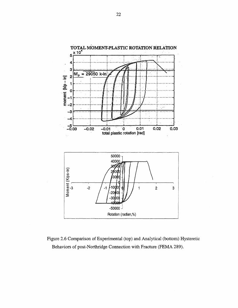
Figure 2.6 Comparison of Experimental (top) and Analytical (bottom) Hysteretic
Behaviors of post-Northridge Connection with Fracture (FEMA 289) ............ 22
Figure 3.1 Measured Moment-Rotation Behavior of T-stub Partially Restrained
Connection, Beam: W21X44, Column: W14X145 (Swanson, 1999) .............. 40
Figure 3.2 Details ofT-Stub Connection (Beam: W21X44, Column: W14XI45) ............ 40
Figure 3.3 A Representative Ductile Beam-Column Connection Behavior of 3-Story
Building (120'XI80') under 2% 50 Years Ground Motion (Beam: W24X117,
Column: WI4x283) ............................................................................................ 41
Figure 3.4 Assumptions for Equation 3.2 (EI-Tawil et al, 1999) ....................................... 41
Figure 3.5 A Representative Tri-Linear Rotational Element to Model the Behavior of
Panel Zone .......................................................................................................... 42
Figure 3.6 Typical Steel Stress-Strain Curves (Solid line) and the Idealized Elastic-Plastic
Steel Stress-Strain Curve (Dashed line) ............................................................. 42
Figure 3.7 Typical Demand Curve of a Building ................................................................ 43
Figure 3.8 Typical IDA Curves of a Building ..................................................................... 43
Figure 3.9 Ground Motion Time History ofLA21 (Top) and LA22 (Bottom) ................. 44
Figure 3.10 Elastic Spectral Acceleration ofLA21 (Top) and LA22 (Bottom) ................... 44
Figure 3.11 Nine Plan Configurations of 3-Story and 12-Story Buildings (Bold Lines
Represent the Moment Frames) ......................................................................... 45
xiv
Figure 3.12 Finite Element Model of a 3-Story Building (Bold Lines Represent the
Moment Frames) ................................................................................................. 46
Figure 3.13 Finite Element Model of a 12-Story Building (Bold Lines Represent the
Moment Frames) ................................................................................................. 46
Figure 4.1 Examples of the post-Northridge Connection Response (Beam Size: W24X207,
with Fracture, Residual Moment = 10% of Plastic Moment) ........................... 70
Figure 4.2 Examples of the post-Northridge Connection Response (Beam Size: W24X207,
with Fracture, Residual Moment = 10% of Plastic Moment) ........................... 71
Figure 4.3 Examples of the post-Northridge Connection Response (Beam Size: W24X279,
without Fracture) ................................................................................................ 72
Figure 4.4 The First Three Modes of a 3-Story Building ................................................... 73
Figure 4.5 The First Three Modes of a 3-Story Building (1bay_interior_1bay_interior) .. 74
Figure 4.6 The Representative First Three Modes of a 12-Story Building ........................ 75
Figure 4.7 The First Three Modes of a 12-Story Building (lbay_interior_1bay_interior).76
Figure 4.8 Roof Displacement Histories of 3-Story Buildings, X-Direction .................... 77
Figure 4.9 Roof Displacement Histories of 3-Story Buildings, X-Direction ..................... 78
Figure 4.10 Roof Displacement Histories of 3-Story Buildings, X-Direction ..................... 79
Figure 4.11 Roof Displacement Histories of 3-Story Buildings, Y-Direction ..................... 80
Figure 4.12 Roof Displacement Histories of 3-Story Buildings, Y-Direction ..................... 81
Figure 4.13 Roof Displacement Histories of 3-Story Buildings, Y-Direction ..................... 82
Figure 4.14 Roof Displacement Histories of 3-Story Buildings, Rotation about Z-axis ..... 83
Figure 4.15 Roof Displacement Histories of 3-Story Buildings, Rotation about Z-axis ..... 84
Figure 4.16 Roof Displacement Histories of 3-Story Buildings, Rotation about Z-axis ..... 85
Figure 4.17 Displacement Time Histories of 12-Story Buildings, X-Direction ................... 86
Figure 4.18 Displacement Time Histories of 12-Story Buildings, Y-Direction ................... 87
Figure 4.19 Displacement Time Histories of 12-Story Buildings, Rotation about Z-Axis .. 88
Figure 4.20 Time History of Roof Displacement of a Building with and without
Considering Panel Zone Response (Bold Line Denotes a Building without
Panel Zone Modeling) ........................................................................................ 89
xv
Figure 4.21 Comparison of MCDR of a Building with/without Considering Panel Zone
Response ............................................................................................................. 90
Figure 4.22 Response Time History of the Panel Zone ........................................................ 90
Figure 4.23 Probabilistic MCDR Demand Curve of a 3-Story Building with pre-Northridge
Connections (upper) and post-Northridge Connections (lower). Solid and
Dashed Lines Indicate Performance Curve with and without Consideration of
Epistemic Uncertainty. 0 Indicates the Median Value ..................................... 91
Figure 4.24 IDA Curves of pre-Northridge (left) and post-Northridge (right) Buildings .... 92
Figure 4.25 Building Drift (%) Ratio Capacity against Incipient Collapse with pre
Northridge (left) and post-Northridge (right) Connections Plotted on Log-
Normal Probability Paper ................................................................................... 92
Figure 4.26 Time History of Roof Displacement for Buildings with Brittle and Ductile
Connections (Bold Line Represents the Building with Brittle Connection) .... 93
Figure 4.27 An IDA Curve under SAC Ground Motions, LA25 and LA26 ....................... 94
Figure 4.28 Time History of Roof Displacement for Buildings with Different Column
Properties ............................................................................................................ 94
Figure 4.29 A Typical Response of a Column with Nonlinear Material Property ............... 95
Figure 4.30 Probabilistic MCDR Demand Curve of 3-Story Buildings. Solid and Dashed
Lines Indicate Performance Curve with and without Consideration of
Epistemic Uncertainty. 0 Indicates the Median Value ..................................... 96
Figure 4.31 Probabilistic MCDR Demand Curve of 3-Story Buildings. Solid and Dashed
Lines Indicate Performance Curve with and without Consideration of
Epistemic Uncertainty. 0 Indicates the Median Value ..................................... 97
Figure 4.32 Probabilistic MCDR Demand Curve of 3-Story Buildings. Solid and Dashed
Lines Indicate Performance Curve with and without Consideration of
Epistemic Uncertainty. 0 Indicates the Median Value ..................................... 98
Figure 4.33 IDA Curves of 3-Story Buildings (Solid Points Represent Collapse Points) ... 99
Figure 4.34 IDA Curves of 3-Story Buildings (Solid Points Represent Collapse Points). 100
Figure 4.35 IDA Curves of 3-Story Buildings (Solid Points Represent Collapse Points). 101
xvi
Figure 4.36 IDA Curves of 3-Story Buildings (3bay_3bay) with 2-D Modeling (Ten
Elastic-Plastic Elements in One Story) ............................................................ 102
Figure 4.37 IDA Curves of 3-Story Buildings (3bay_3bay) with 2-D Modeling (One
Lumped-Plasticity Element in One Story) ....................................................... 102
Figure 4.38 IDA Curves of 3-Story Buildings (3bay_3bay) with 2-D Modeling-(l) ........ 103
Figure 4.39 IDA Curves of 3-Story Buildings (3bay_3bay) with 2-D Modeling-(2) ........ 103
Figure 4.40 Probabilistic MCDR Demand Curve of 12-Story Buildings. Solid and Dashed
Lines Indicate Performance Curve with and without Consideration of
Epistemic Uncertainty. 0 Indicates the Median Value ................................... 104
Figure 4.41 IDA Curves of 12-Story Buildings (Solid Points Indicate Collapse Points) .. 105
Figure 4.42 The Plan View of Two Basic Configurations, 120'XI80' (upper) and
I80'X270' (lower) ............................................................................................ 106
Figure 4.43 Time History of the 2-D Roof Displacement of IBC2000 3-Story Buildings
with Ductile Connections and Floor Area of I20'x180' and I80'x270' ........ 106
Figure 5.1 p Factors (based on RR Factor) of 3-Story Buildings ...................................... 129
Figure 5.2 p Factors (based on the NEHRP 2003) of 3-Story Buildings under Excitations
in Y-Direction ................................................................................................... 130
Figure 5.3 p Factors (based on RR Factor) of 12-Story Buildings .................................... 131
Figure 5.4 Residuals Plot (left) and Q-Q Plot (right) of the Regression Model. .............. 132
Figure 5.5 Residuals Plot (left) and Q-Q Plot (right) of the Regression Model. .............. 132
Figure 5.6 Regression Plots of MCDR on BSA for I2-Story Buildings .......................... 133
Figure 5.7 Regression Plots of MCDR on SBSA for 12-Story Buildings ........................ 134
Figure 5.8 Incipient Collapse Fragility Curves of 3-Story Buildings ............................... 135
Figure 5.9 Incipient Collapse Fragility Curves of I2-Story Buildings ............................. 135
Figure A.I Configurations of Series System (left) and Parallel System (right) ................ 145
Figure A.2 Rind versus the Number of Components in a Parallel System ......................... 145
1
CHAPTER 1 INTRODUCTION
1.1 Background
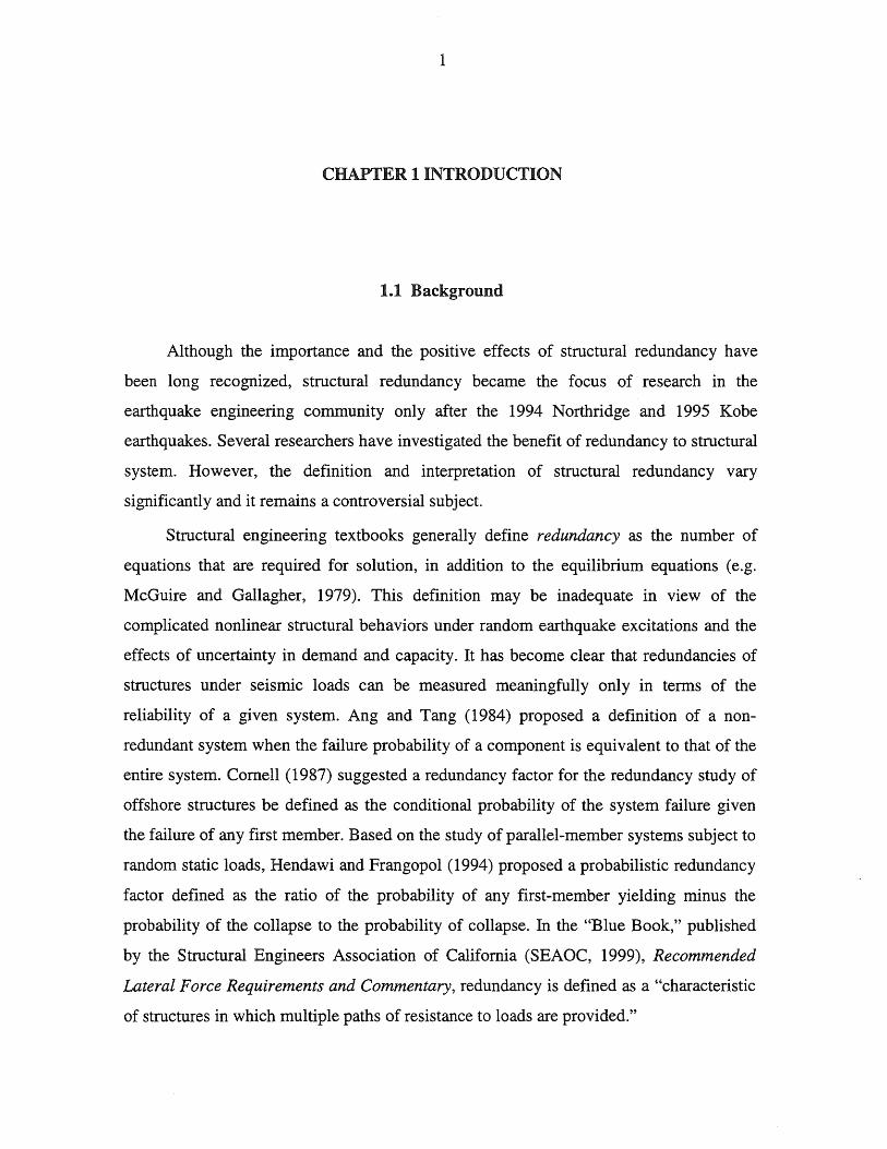
Although the importance and the positive effects of structural redundancy have
been long recognized, structural redundancy became the focus of research in the
earthquake engineering community only after the 1994 Northridge and 1995 Kobe
earthquakes. Several researchers have investigated the benefit of redundancy to structural
system. However, the definition and interpretation of structural redundancy vary
significantly and it remains a controversial subject.
Structural engineering textbooks generally define redundancy as the number of
equations that are required for solution, in addition to the equilibrium equations (e.g.
McGuire and Gallagher, 1979). This definition may be inadequate in view of the
complicated nonlinear structural behaviors under random earthquake excitations and the
effects of uncertainty in demand and capacity. It has become clear that redundancies of
structures under seismic loads can be measured meaningfully only in terms of the
reliability of a given system. Ang and Tang (1984) proposed a definition of a non
redundant system when the failure probability of a component is equivalent to that of the
entire system. Cornell (1987) suggested a redundancy factor for the redundancy study of
offshore structures be defined as the conditional probability of the system failure given
the failure of any first member. Based on the study of parallel-member systems subject to
random static loads, Hendawi and Frangopol (1994) proposed a probabilistic redundancy
factor defined as the ratio of the probability of any first-member yielding minus the
probability of the collapse to the probability of collapse. In the "Blue Book," published
by the Structural Engineers Association of California (SEAOC, 1999), Recommended
Lateral Force Requirements and Commentary, redundancy is defined as a "characteristic
of structures in which multiple paths of resistance to loads are provided."
2
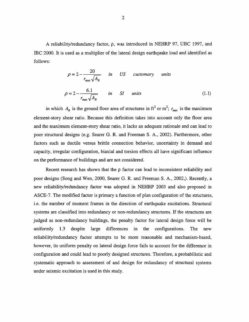
A reliability/redundancy factor, p, was introduced in NEHRP 97, VBC 1997, and
IBe 2000. It is used as a multiplier of the lateral design earthquake load and identified as
follows:
20 P = 2 - -----,,=
rmax ~AB
p = 2- 6.1 rmax~AB
in US customary units
in SI units (1.1)
in which AB is the ground floor area of structures in ft2 or m2; r max is the maximum
element-story shear ratio. Because this definition takes into account only the floor area
and the maximum element-story shear ratio, it lacks an adequate rationale and can lead to
poor structural designs (e.g. Searer G. R. and Freeman S. A., 2002). Furthermore, other
factors such as ductile versus brittle connection behavior, uncertainty in demand and
capacity, irregular configuration, biaxial and torsion effects all have significant influence
on the performance of buildings and are not considered.
Recent research has shown that the p factor can lead to inconsistent reliability and
poor designs (Song and Wen, 2000, Searer G. R. and Freeman S. A., 2002,). Recently, a
new reliability/redundancy factor was adopted in NEHRP 2003 and also proposed in
ASCE-7. The modified factor is primary a function of plan configuration of the structures,
i.e. the number of moment frames in the direction of earthquake excitations. Structural
systems are classified into redundancy or non-redundancy structures. If the structures are
judged as non-redundancy buildings, the penalty factor for lateral design force will be
uniformly 1.3 despite large differences in the configurations. The new
reliability/redundancy factor attempts to be more reasonable and mechanism-based,
however, its uniform penalty on lateral design force fails to account for the difference in
configuration and could lead to poorly designed structures. Therefore, a probabilistic and
systematic approach to assessment of and design for redundancy of structural systems
under seismic excitation is used in this study.
3
1.2 Previous Research on Structural Redundancy
De et al (1989) and Gollwitzer and Rackwitz (1990) have conducted extensive
studies on the redundancy of simple parallel systems with random capacity under random
static loads. They found that the redundancy of a system can be significantly improved by
using a larger number of members with a low strength correlation among the members, a
small ratio of variability of load to member resistance and adequate member ductility
capacity. Since nonlinear response and load redistribution after member failures for
structural systems under dynamic earthquake excitations become considerably more
complex than in a simple parallel system under static loads, the investigation of such
behaviors is essential in the evaluation of the building redundancy.
Bertero and Bertero (1999) utilized the concept of the redundancy degree, defined
as the number of plastic hinges of the structural system that fails when the structure
collapses, to investigate the redundancy of frame structures in static and dynamic
analyses. Effects of over-strength, coefficients of variation of demand and capacity,
plastic rotation capacity (finite or infinite) on failure probability and redundancy of frame
structures were investigated. They found that a reduction factor R due to redundancy
cannot be established independently of the over-strength and ductility of the system.
However, they did not suggest a way to incorporate redundancy effect into procedures of
structural design.
Whittaker and Hart, et al. (1999) used the reliability index or safety index (Ang and
Tang, 1984) to investigate the redundancy of structures under earthquake excitations
assumed to be deterministic. Assuming the strength and stiffness of components of a
structural system are identical, they found that the benefit of structural redundancy
depends on the correlation of components. Further, they were highly critical of the p
factor, defined in NEHRP 97, being based on the floor area and which does not take into
account the relative stiffness and strength of vertical seismic framing. They proposed four
lines of strength- and deformation-compatible vertical seismic framing in each principle

4
direction of a building as the minimum for adequate redundancy. A draft redundancy
factor, which varies as a function of the number of the vertical lines, was also proposed.
Wang and Wen (2000) developed a smooth hysteretic model to reproduce the
moment-rotation behavior of brittle connections of pre-Northridge steel buildings. A 3-D
building model was developed to account for the effects of bi-axial excitation and torsion
motions under seismic loadings. Moreover, a uniform-risk redundancy factor was
developed to calculate the required design base-shear force for structures of different
degrees of redundancy to satisfy a uniform reliability requirement. Song and Wen (2000)
investigated the redundancy of special moment resisting frames (SMRF) in terms of the
system reliability under SAC ground motions. Key factors considered included structural
configuration (number of moment resisting frames), uncertainty in demand (in terms of
column drift ratio) and uncertainty in material strength. The study included 3-D ductile
SMRF of three and nine stories and equal floor area and strength, with a different
numbers of bays and different beam and column sizes. In addition, to investigate the
effect of brittle versus ductile connections, brittle SMRF of a different number of bays,
equal strength and floor area were analyzed.
Although the proceeding research examined several important factors that affect
building redundancy. The effects of other factors such as different floor areas, irregular
plan configuration, role of gravity frames and the behavior of post-Northridge
connections remain unclear and need to be investigated for performance evaluation and
design of buildings.
1.3 Objective and Scope
The objective of this study is to develop further understanding of structural
redundancy and a risk-consistent redundancy factor for design. To achieve this objective,
a systematic evaluation of redundancy in buildings under seismic excitation, considering
factors in addition to those previously investigated, is required. The research scope is
listed as follows:
5
1. Identification 'and quantification of important redundancy contributing factors
for representative special moment resisting frames (SMRF). For this purpose,
investigations of potential redundancy contributing factors such as floor area,
story number, floor configuration, and gravity frame are carried out. Both
brittle and ductile connections are considered.
2. Development of a risk-consistent redundancy factor for the improvement in
design for redundancy which may lead to a more rational design provision.
To achieve the objectives, two core areas need to be considered: accurate modeling
of the structural response and adequate treatment of uncertainty in the system demand
and capacity. Accuracy of the analysis of inelastic structural responses under seismic
loads depends largely on the modeling of buildings. The following structural modeling
issues are of particular relevance to this study.
1. Examining the effects of the interior frames, e.g. gravity frames, on the
redundancy of buildings. Gravity frames, primarily designed to resist vertical
loads, are known to contribute to lateral resistance. Their influence on building
performance needs further investigation.
2. Accurate estimation of connection capacity against fracture is crucial due to its
significant influence on building performance.' Structural element rotation (or
rotational ductility) is commonly used as a damage measure. In the FEMAISAC
project, a series of experiments were conducted to investigate the performance
of steel moment frame connections, including both pre-Northridge and post
Northridge connections. The rotational capacity of connections was estimated
by a least squares fit to experimental data and reported in FEMA 355D. This
study incorporates the experimental data into Bouc-Wen model to reproduce the
inelastic behavior of beam-column connections and their uncertainties.
3. Frames without fully restrained connections, e.g., T -stub connections, the
stiffness of these connections needs to be taken into account. Partially restrained
(PR) connections usually have significant rotation within the connection before
the connection develops its ultimate resistance, and the stiffness of PR
6
connections varies greatly; therefore, realistic modeling of connections based on
experiments is important when investigating the redundancy of structures.
Investigation of building behavior under earthquakes must include effects of
uncertainty. Randomness as well as modeling errors in ground motion intensity,
displacement demand and displacement capacity are crucial when evaluating building
performance. SAC phase-2 ground motions (Somerville, 1997) corresponding to 2% and
10% exceedance probability in 50 years are used in this study. The uncertainty in demand
can be determined in terms of the maximum column drift ratio (MCDR) via time history
analyses. The uncertainty in capacity may arise due to ground motion (record-to-record
uncertainty), member properties (material and nonlinear behaviors) and other factors such
as workmanship. Incremental Dynamic Analysis (IDA) is utilized for the capacity
analysis against incipient collapse. Further, the Monte-Carlo simulation is used to consider
the effects of uncertainty due to material properties, the capacity of brittle connections of
structural performance.
1.4 Organization
Chapter 2 introduces the Bouc-Wen smooth connection-fracture hysteresis model.
This model is then incorporated with ABAQUS computer program as a user-defined
element (DEL) to account for inelastic and degrading connection behavior of steel
moment frames. The experimental results of connection capacity, which are documented
in FEMA 355D, are implemented in this DEL to take the potential brittle connection
behaviors into account.
Chapter 3 introduces the modeling and design of the buildings. mc 2000 (NEHRP
97) is used as the basis to design all buildings. Buildings are assumed to be located in the
Los Angles downtown area. Inelastic yielding of the girder of moment frames is assumed
to be confined to discrete hinge regions located at the ends of beam elements (lumped
plasticity), where the Bouc_ Wen model is implemented to describe inelastic connection
behaviors. The columns of moment resisting frames are modeled using beam elements
7
with nonlinear material property. Shell elements are used to model the flexible floor.
Gravity frames are also designed and included in the finite element model while the
connections of gravity frames are assumed to have no rotational resistance (e.g., a hinge
connection). In addition, an accidental torsional moment produced by horizontal offset in
the center of mass is considered. P-~ effect and the randomness of material and member
properties are considered. Finally, a 3-D finite element model is developed for the
structural system, in which the biaxial interaction, torsional oscillation and brittle beam
column joint failures are investigated.
Chapter 4 consists of response analyses of a series of 3-story and 12-story steel
moment-resisting buildings subjected to ground motions of the SAC Phase 2 project
using the hysteresis and structural models developed in Chapters 2 and 3. In order to
examine the effects of floor configurations on building performance, nine different floor
configurations, commonly used in practice, are investigated and compared with the
results of the uniform-risk redundancy factor in chapter 5. Because the buildings are
under biaxial excitations, a definition of biaxial spectral acceleration is proposed
considering concurrently the dynamic properties in the two principal directions of
buildings. It has been found that the biaxial spectral acceleration (BSA) and the
maximum column drift ratio (MCDR), which will be used as ground motion intensity
measures respectively, can be modeled as random variables with log-normal distribution.
The investigation includes the demand and capacity analyses for each building. A suite
of time history analysis determines the displacement demand (Dd). As proposed by
Wang and Wen (2000), the median MCDR responses multiplied by the correction factor
for the capacity uncertainty at the two hazard levels (e.g. 10% and 2 % in 50 yrs) is used
to establish the probabilistic drift demand curve. The displacement capacity (Dc) is
determined by performing Incremental Dynamic Analyses (IDA). Details of the IDA are
described in Chapter 3.
Buildings of equal floor aspect ratios and equal number of moment-resisting
frames, but with different floor areas, are also included in this chapter to investigate the
effects of floor area on building performance.
8
In Chapter 5, a framework is presented for evaluation of structural reliability and
redundancy against specified limit states such as incipient collapse. Structural reliability
can be determined in terms of the displacement demand versus capacity. In this study, the
maximum column drift ratio (MCDR) or biaxial spectral acceleration (BSA) is used to
measure both demand and capacity. Both randomness and modeling errors (aleatory and
epistemic uncertainties) in the demand and capacity are considered. The uniform-risk
redundancy factor (RR)' for designing a uniform reliability level for buildings of different
redundancies, is constructed, following Wang and Wen (2000). This factor is also used to
evaluate the redundancy of a given structural system. Comparisons between the p factor
in NEHRP 97, in NEHRP 2003 and the RR factor are carried out. Based on the results of
RR factor derived from different buildings, statistic analyses are conducted and a practical
relationship between structural redundancy and plan configuration is proposed for
possible application on codified design. The 50-year limit state probability and the
fragility curve are also calculated for each building.
Chapter 6 summarizes the conclusions of this study and recommendations for
future research.

9
CHAPTER 2 MODELING OF BEAM-COLUMN CONNECTIONS
2.1 Introduction
Although only a few buildings collapsed in the 1994 Northridge earthquake,
hundreds of welded-flange-bolted-web connections of steel moment frames failed due to
fracture. Because the resistance of moment frames to seismic excitations is largely
dependent on the performance of the connections, understanding and improving
connection performance became an important issue. In order to make the discussion clear
throughout this study, connection is referred to the portion that beam and column are
connected and does not include the panel zone. The SAC joint venture, which includes
the Structural Engineers Association of California, the Applied Technology Council, and
the California Universities for Research in Earthquake Engineering, then conducted a
series of tests of pre- and post-Norridge connections to investigate the behavior of
connection failures. The rotational capacity of connections was used as the basis to
describe the connection capacity and was estimated by a least squares fit to experimental
data (FEMA 355D). The plastic rotational capacity at failure, 8p, is defined as the
maximum plastic rotation at which initial fracture occurred or where the resistance
dropped below 80% of the plastic moment capacity calculated from the measured yield
stress of the steel. The results shown indicate that the plastic rotational capacity is highly
random and largely dependent on the depth of beam. Therefore, a probabilistic approach
should be used to predict the failure of connection capacity.
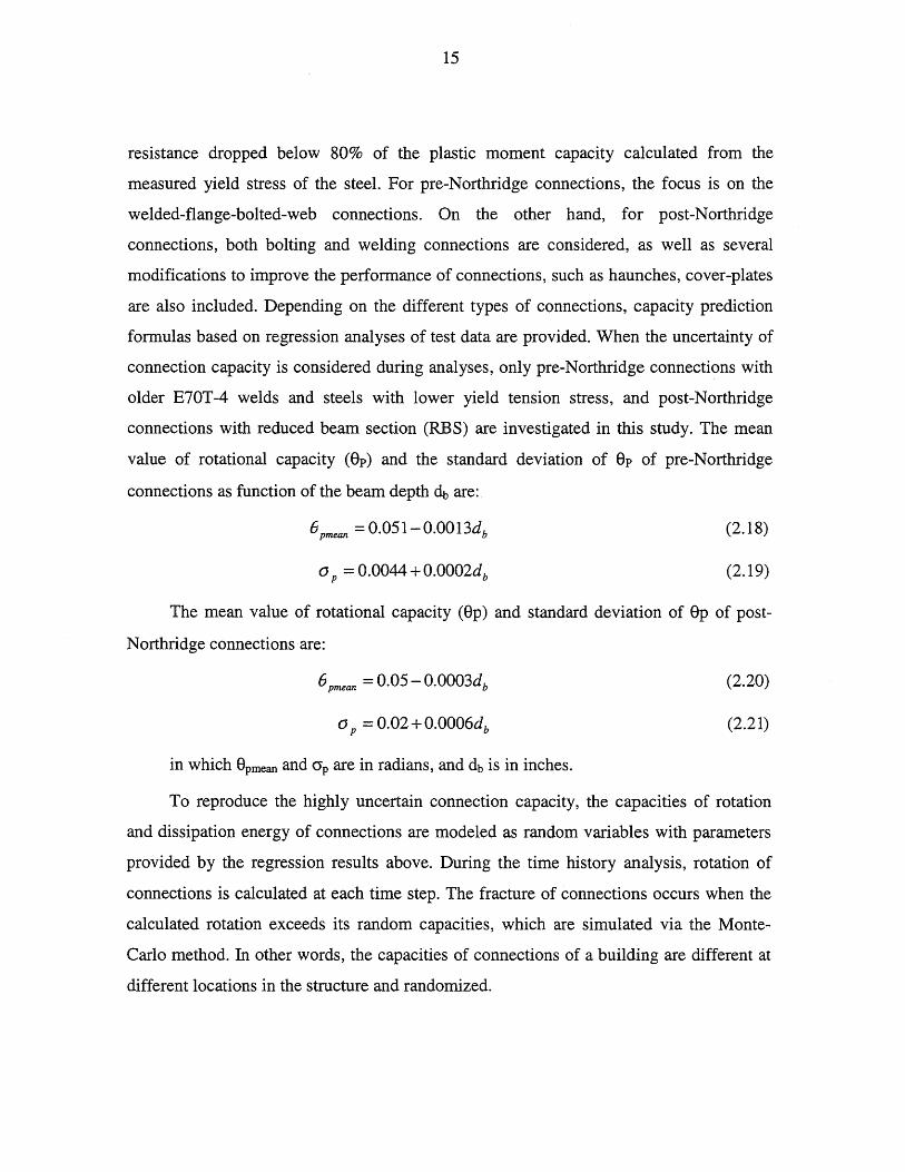
Shi (1997) proposed a piecewise-linear model to reproduce the behavior beam
column connections (Figure 2.1), and incorporated it into the DRAIN-2DX computer
program as an additional element type. A number of controlling parameters and rules are
used in this model in order to match the hysteresis loops derived from experimental data.
Because this model was developed primarily as an extension to the DRAIN-2DX,
10
extension to 3-D analyses is difficult. Wang and Wen (2000) developed a 3-D finite
element program, in which the Bouc-W en model is used as the basis to describe the
inelastic behavior of beam-column connections. The Bouc-W en model developed in
Wang's program is used in this study and incorporated into the ABAQUS computer
program to take advantage of many ABAQUS built-in elements and a variety of analyses
such as large displacement analysis, where geometric nonlinearity is considered.
The Bouc-W en model will be briefly described in the following. The formulation
of an ABAQUS user-defined-element (DEL) is also described, and also how the SAC
experimental results are implemented into the DEL.
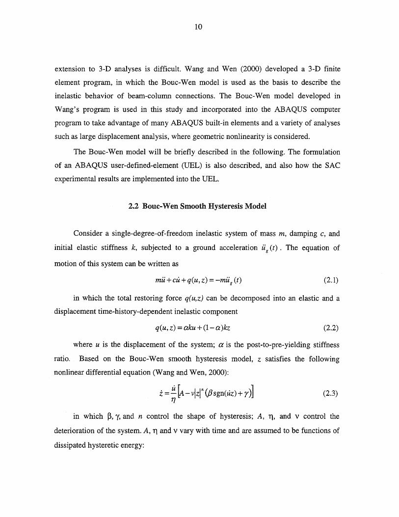
2.2 Boue .. Wen Smooth Hysteresis Model
Consider a single-degree-of-freedom inelastic system of mass m, damping c, and
initial elastic stiffness k, subjected to a ground acceleration ilg (t). The equation of
motion of this system can be written as
mil + cu + q(u, z) = -mil g (t) (2.1)
in which the total restoring force q( u,z) can be decomposed into an elastic and a
displacement time-history-dependent inelastic component
q(u,z) = aku +(1-a)kz (2.2)
where u is the displacement of the system; a is the post-to-pre-yielding stiffness
ratio. Based on the Bouc-Wen smooth hysteresis model, z satisfies the following
nonlinear differential equation (Wang and Wen, 2000):
z = u [A - vlzln (j3 sgn(uz) + r)]
1] (2.3)
in which ~,,¥, and n control the shape of hysteresis; A, 'Tl, and v control the
deterioration of the system. A, 'Tl and v vary with time and are assumed to be functions of
dissipated hysteretic energy:

11
(2.4)
in which Ao, 110, Vo are initial values and ()A, ~, Ov are the rates of degradation. E is
the normalized dissipated hysteretic energy and calculated as follows:
I-aft E=-- kzudt FI1 0
(2.5)
in which F = the yield force and 11 = yield displacement. To see the effect of the
parameters above on the ultimate hysteretic displacement, Zu ' when z reaches the
ultimate value, i approaches zero, Ii and z have the same sign. Therefore, Zu can be
obtained as a function of the parameters as follows:
(2.6)
1
z, =[v(p~rJ (2.7)
Hysteresis loop pinching can be included by incorporating a time-dependent "slip
lock" element (Baber and Noori, 1985). The following function is used in this study as a
slip-lock element, which was proposed by Wang and Wen (2000).
2
(2.8)
sgn(u)~-q f(z)= T2 ~exp _! ___ z.;;;;....u_ "ri (j 2 (j
where the parameter a controls the length of the pinching; (j controls the sharpness
of pinching; q controls the "thickness" of pinching area. The following function for a was
also recommended by Wang (2000):
(2.9)
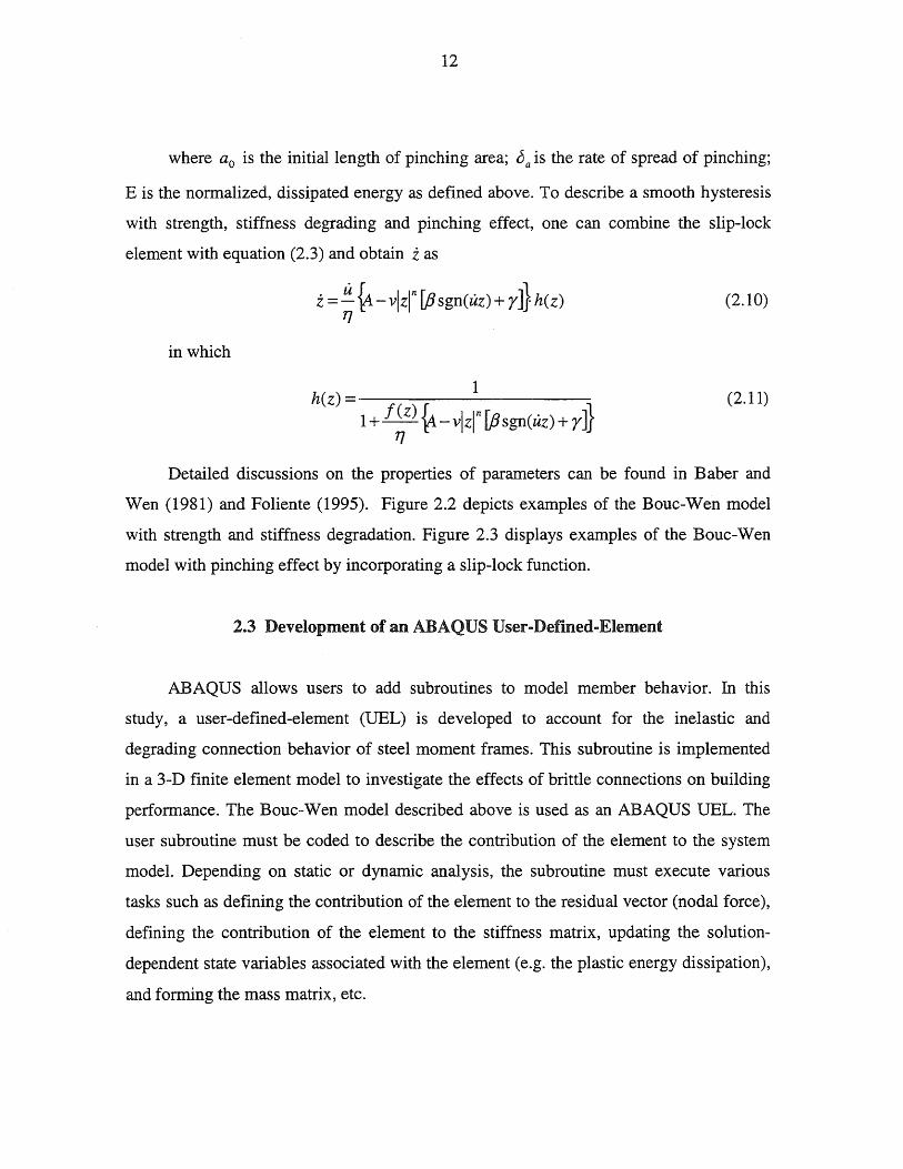
12
where ao is the initial length of pinching area; ~ a is the rate of spread of pinching;
E is the normalized, dissipated energy as defined above. To describe a smooth hysteresis
with strength, stiffness degrading and pinching effect, one can combine the slip-lock
element with equation (2.3) and obtain i as
in which
i = u {4. - vlzln [B sgn(uz) + r]} h(z) 7]
h(z) = _____ 1 ____ _
1+ fez) ~-vlzln[Bsgn(uz)+r]} 7]
(2.10)
(2.11)
Detailed discussions on the properties of parameters can be found in Baber and
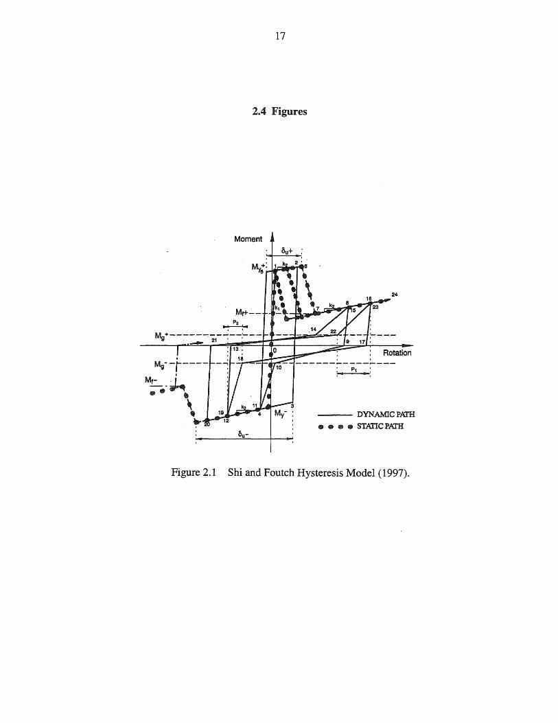
Wen (1981) and Foliente (1995). Figure 2.2 depicts examples of the Bouc-W en model
with strength and stiffness degradation. Figure 2.3 displays examples of the Bouc-W en
model with pinching effect by incorporating a slip-lock function.
2.3 Development of an ABAQUS User-Dermed-Element
ABAQVS allows users to add subroutines to model member behavior. In this
study, a user-defined-element (VEL) is developed to account for the inelastic and
degrading connection behavior of steel moment frames. This subroutine is implemented
in a 3-D finite element model to investigate the effects of brittle connections on building
performance. The Bouc-Wen model described above is used as an ABAQVS VEL. The
user subroutine must be coded to describe the contribution of the element to the system
model. Depending on static or dynamic analysis, the subroutine must execute various
tasks such as defining the contribution of the element to the residual vector (nodal force),
defining the contribution of the element to the stiffness matrix, updating the solution
dependent state variables associated with the element (e.g. the plastic energy dissipation),
and forming the mass matrix, etc.
13
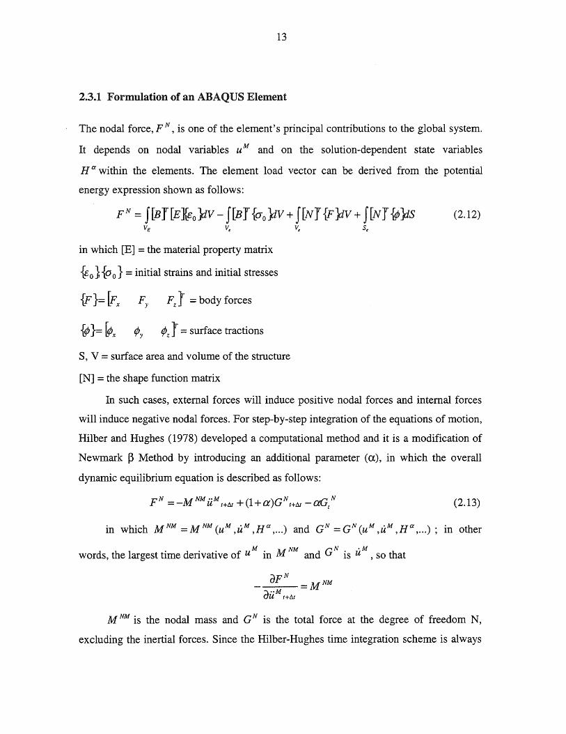
2.3.1 Formulation of an ABAQUS Element
The nodal force, pN, is one of the element's principal contributions to the global system.
It depends on nodal variables u M and on the solution-dependent state variables
H a within the elements. The element load vector can be derived from the potential
energy expression shown as follows:
in which [E] = the material property matrix
{eo} {oo } = initial strains and initial stresses
{g)}= ~x ¢y ¢z Y = surface tractions
S, V = surface area and volume of the structure
[N] = the shape function matrix
(2.12)
In such cases, external forces will induce positive nodal forces and internal forces
will induce negative nodal forces. For step-by-step integration of the equations of motion,
Hilber and Hughes (1978) developed a computational method and it is a modification of
Newmark ~ Method by introducing an additional parameter (a), in which the overall
dynamic equilibrium equation is described as follows:
P N MNM .. M (1 )GN aG N = - U t+& + + a t+& - t (2.13)
in which MNM =MNM(uM,itM,Ha, ... ) and GN =GN(UM,itM,H a, ... ); in other
words, the largest time derivative of uM
in M NM and GN
is uM , so that
_ (JpN =M NM (Jii M
t+M
M NM is the nodal mass and G N is the total force at the degree of freedom N,
excluding the inertial forces. Since the Hilber-Hughes time integration scheme is always
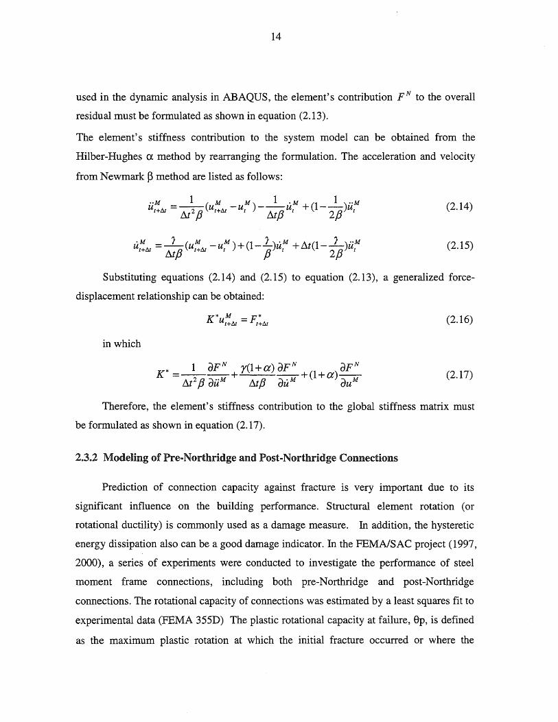
14
used in the dynamic analysis in ABAQUS, the element's contribution F N to the overall
residual must be formulated as shown in equation (2.13).
The element's stiffness contribution to the system model can be obtained from the
Hilber-Hughes a method by rearranging the formulation. The acceleration and velocity
from Newmark ~ method are listed as follows:
•• M 1 (M M ) 1. M (1 1) .. M ut+& = --2 - u t+& -ut ---ut + -- u t
f!,.t {3 f!,.t{3 2{3 (2.14)
(2.15)
Substituting equations (2.14) and (2.15) to equation (2.13), a generalized force
displacement relationship can be obtained:
K * M F* ut+& = t+& (2.16)
in which
(2.17)
Therefore, the element's stiffness contribution to the global stiffness matrix must
be formulated as shown in equation (2.17).
2.3.2 Modeling of Pre-Northridge and Post-Northridge Connections
Prediction of connection capacity against fracture is very important due to its
significant influence on the building performance. Structural element rotation (or
rotational ductility) is commonly used as a damage measure. In addition, the hysteretic
energy dissipation also can be a good damage indicator. In the FEMAISAC project (1997,
2000), a series of experiments were conducted to investigate the performance of steel
moment frame connections, including both pre-Northridge and post-Northridge
connections. The rotational capacity of connections was estimated by a least squares fit to
experimental data (FEMA 355D) The plastic rotational capacity at failure, 8p, is defined
as the maximum plastic rotation at which the initial fracture occurred or where the
15
resistance dropped below 80% of the plastic moment capacity calculated from the
measured yield stress of the steel. For pre-Northridge connections, the focus is on the
welded-flange-bolted-web connections. On the other hand, for post-Northridge
connections, both bolting and welding connections are considered, as well as several
modifications to improve the performance of connections, such as haunches, cover-plates
are also included. Depending on the different types of connections, capacity prediction
formulas based on regression analyses of test data are provided. When the uncertainty of
connection capacity is considered during analyses, only pre-Northridge connections with
older E70T-4 welds and steels with lower yield tension stress, and post-Northridge
connections with reduced beam section (RBS) are investigated in this study. The mean
value of rotational capacity (ep) and the standard deviation of ep of pre-Northridge
connections as function of the beam depth db are:
6pmean = 0.051-0.0013db
o p = 0.0044+0.0002db
(2.18)
(2.19)
The mean value of rotational capacity (ep) and standard deviation of ep of post
Northridge connections are:
6 pmean = 0.05 - 0.0003db
o p = 0.02+0.0006db
in which eprnean and O"p are in radians, and db is in inches.
(2.20)
(2.21)
To reproduce the highly uncertain connection capacity, the capacities of rotation
and dissipation energy of connections are modeled as random variables with parameters
provided by the regression results above. During the time history analysis, rotation of
connections is calculated at each time step. The fracture of connections occurs when the
calculated rotation exceeds its random capacities, which are simulated via the Monte
Carlo method. In other words, the capacities of connections of a building are different at
different locations in the structure and randomized.

16
Once the fracture of a connection has occurred, a bilinear model is used to describe the
post-fracture behavior of this connection with the residual strength of this connection
assumed to be maintained at 10% of the yielding strength. This assumption of 10% will
also be examined in section 4.7.
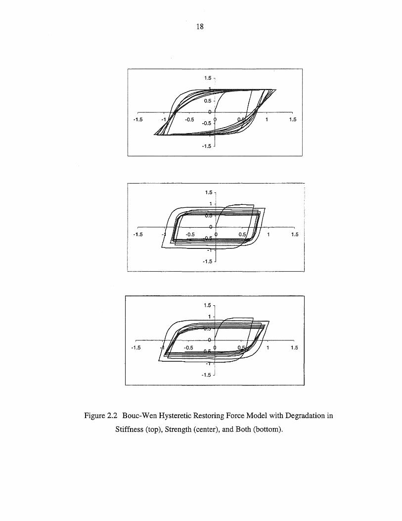
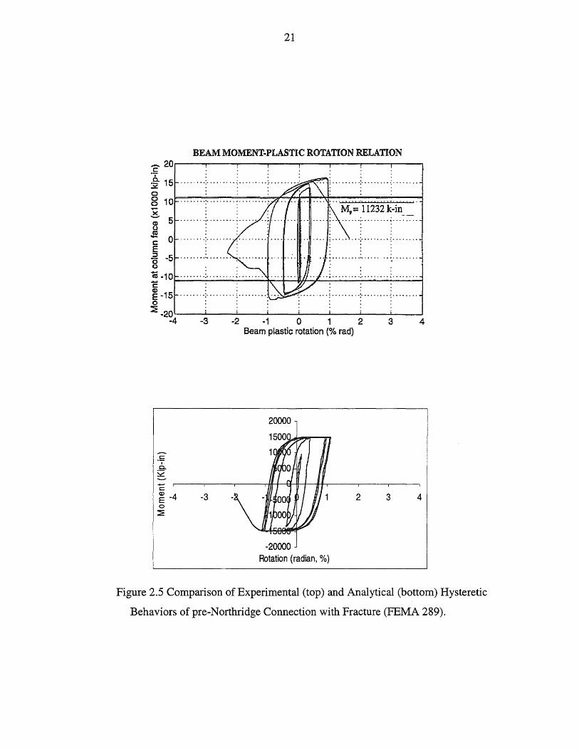
2.3.3 Comparison with Experimental Result
FEMA 289 provides detailed descriptions of experiments including connection
details, applied loading/displacement histories, and cumulative energy dissipations. Both
pre- and post - Northridge connections experimental results are reported in this document.
The employment of exact applied loading histories and laboratory setup used in the
experiment tests will not be attempted, due to the scope of this study, which aims to: (1)
demonstrate the capability of the Bouc-Wen model in reproducing important hysteretic
behavior, such as smooth yielding of hysteresis loops, degrading of strength or stiffness;
and (2) incorporate the Bouc-Wen model into ABAQUS finite program.
A one-story frame with one bay under a harmonic excitation is analyzed to examine
the connection behavior. A comparison of experimental and analytical behaviors of post
Northridge connections without fracture is shown in Figure 2.4. A comparison of
experimental and analytical behaviors of pre- and post-Northridge connections with
fracture is shown in Figure 2.5 and Figure 2.6, respectively. Results shown here indicate
that the proposed model captures the important hysteretic properties of test data.
17
2.4 Figures
Moment
--- : 13 : I 121
Mg--,-----
~-~ .. , ~ ~ ...
24
Rotation
--- DYNAMIC PATH ED ED • ED STATIC PATII
Figure 2.1 Shi and Foutch Hysteresis Model (1997).
18
1.5
-1.5 -0.5 -0.5 1.5
-1.5
1.5
-1.5 1.5
-1.5
-1.5 1.5
Figure 2.2 Bouc-Wen Hysteretic Restoring Force Model with Degradation in
Stiffness (top), Strength (center), and Both (bottom).

19
1.5
-1.5 1.5
-1.5
(1) cr = 10
1.5
-1.5 -1 1.5
-1.5
(2) cr = 15
Figure 2.3 Bouc-Wen Hysteretic Restoring Force Model with Pinching Effect.

20
BEAM MOl\1ENT .. PLASTIC ROTATION RELATION
c= : : " 20 .. " .... -: .......... ~ ......... : .......... :. . .. : ......... : ......... ~ ....... . c. " ~~ .. 32 15 .......... ~ ......... ~ ......... ~ .... ~ .. 8 '" . .E 10 hlp: 11232 k-in .... . .. .. ........ : ....
B 5 . S c: E
i -15 E ~ -20
........ : ......... ,; ....... . · . . · . . ..................................... · . . · . . · . .
.... : .................. : ................. : ............... '0 ~ .............. .. .. .. .. .. .. .. .. ..
~5~----~--------~----~~----~------~--------~----~---------~ -8
"E Q) -8 E o
:::2:
-6 -2 0 2 4 6 8 Beam plastic rotation (% rad)
25000
8
Rotation (radian, %)
Figure 2.4 Comparison of Experimental (top) and Analytical (bottom) Hysteretic
Behaviors of post-Northridge Connection without Fracture (FEMA 289).
21
BEAM MOMENT-PLASTIC ROTATION RELATION _20~--~----~--~--~----~--~----~--~ .E ~ 15 o g 10 ..... ~
CD 5 Jg c 0 E ~ -5 o
••••••• • : •••• , •••• ~ •••• , ••• • :. 4 •••••••• "
· . . · . . · . .
m .10 c F-------------~-+~~~--~----~~--~
~ -15 ....... -: ......... ~ ........ '. .. . .: ......... : ......... :. " ....... : ....... . o ::::::: ~-20~--~· ----:~--~:----~:----~.----~:----~:--~
-4 -3
.!:: I
c.. 52 -c E -4 o
:::a:
-3
~2 ·1 0 1 2 3 4 Beam plastic rotation (% rad)
20000
2 3 4
-20000 Rotation (radian, %)
Figure 2.5 Comparison of Experimental (top) and Analytical (bottom) Hysteretic
Behaviors of pre-Northridge Connection with Fracture (FEMA 289).
22
· . . · . . 4. ,.,., ..•... ~ ..•...• ~ •.. ~' .••.. ";'.: .. : .. ;.,.
., . .. ". "
'3 '~.' ..•..... ': ........... :'. '.' . . .. . . . . ; .•. ; .. ~ .. :.: ....••.. ~ ~':':. .. . •...• ;M' ~ 29050. ·k .. iA:: ....... ...:(.:. " : :s 2· _P -": '.' ..... ~ .. ... \~. . ........ :.~ .. ,,:., ..... :- ...... ,., . ".
"" "" "" ""
" " " " " " " " " ":" " " " " " " "" "~""" ."" ": ~ , t ~" """ ",. ." ~:. "... """"""" ~ •• " " " " " " " " ~ "
· . .. . " ... " ......... ::- ........... " .......... . . , , . .• .
-3 .......... : .. ' .......... :.' .....•... ' , . . . .
-4. . .. : ..... ,,""""""" -:""""" ... " .. ".~. " ... """" "" . '" " " , . .
-5~----~----~~~~~~~~--~--~~ -0.03 -0.02 -O~01··:·· b 0.010.020.03
-.5 I
(J)
c.. S2
total plastic rotation [rad]
50000
- ~----~---+~r-~~~~~----~-----.
-2 2 3
-50000 Rotation (radian, % )
Figure 2.6 Comparison of Experimental (top) and Analytical (bottom) Hysteretic
Behaviors of post-Northridge Connection with Fracture (FEMA 289).

23
CHAPTER 3 MODELING AND DESIGN OF BllLDINGS
3.1Introduction
For performance evaluation a structural engineer needs to accurately estimate the
response demand and the capacity of buildings under ground motion excitation of a given
level, e.g. corresponding to a hazard of a given probability. Since structures generally go
into an inelastic range under severe seismic excitations, the accuracy of the demand and
the capacity analysis depend largely on the nonlinear structural modeling. The important
system demand and capacity contributing factors, namely, uncertainty in material
properties and members, randomness in ground motions, and inelastic structural member
behaviors including brittle connection failure, also need to be considered in the structural
analyses. Details of modeling and design of buildings is described in the following.
A building of regular, symmetric configuration and uniform mass distribution may
be modeled as a 2-D frame structure without losing much of accuracy. On the other
hand, for buildings with non-uniform mass distribution or with asymmetrically fractured
beam-column connections, the biaxial interaction of buildings may have significant
effects on the response of buildings under seismic excitation. Therefore, a 3-D finite
element model based on ABAQUS is developed to take the biaxial interaction of
buildings into consideration. In a.c:l9.!tiQI!, the gravity frames are also included in the 3-D
model; hence, their effects on the building performance can be investigated more
accurately than a 2-D model. The beam column connections of the gravity frames are
assumed to be simple hinges in this study following Yun (2000).
Many analyses of steel frames assume the floor diaphragms to be rigid and that
plastic deformation can occur only in columns. The recent design philosophy, however,
encourages strong-column, weak-beam designs to prevent inelastic distortions from
occurring in the columns. Additionally, with respect to the effects of connection
24
fractures, the girders need to be modeled with reasonable flexibility and moment-resisting
capacity. It is necessary, therefore, that the floor diaphragms remain flexible in the
modeling of building structures. Shell elements are then used to model the flexible
diaphragm in this study.
In principle, the yielding locations of a structure can be formed at any high-stress
regions. The lateral displacement is dominated by the deformation of moment frames in
a SMRF, particularly, at the locations near the beam-to-column connections. Thus, this
study will assume the inelastic deformation of structures to concentrate at regions
adjacent to beam-column connections and modeled as discrete inelastic hinges at girder
ends (lumped plasticity), where the Bouc-Wen model is used to describe the hysteretic
behavior as depicted in Chapter 2. Also, to consider the inelastic deformation in column
of moment frames, a perfect elastic-plastic material is used in the finite element analyses.
Based on Krawinkler's research (2000), a tri-linear rotational spring is used to simulate
the panel behavior, and then investigate its effect on the performance of SMRF under
seismic excitations. P-Ll effect and the randomness of materials and member properties
are also considered in the analyses.
3.2 Dynamic Time History Analysis Procedure
Inelastic dynamic time history analysis is performed to evaluate the probabilistic
demand and capacity of a building. The step-by-step integration scheme of the equations
of motion, developed by Hilber and Hughes (1978), is used in this study. It is a
modification of Newmark ~ Method by introducing an additional parameter (a ), and in
order to maintain the numerical stability, the integration time steps are allowed to vary
during the analysis. This is of particular importance when the structure is yielding with
large displacement and fracture. A smaller time step is necessary to avoid numerical
singularity and to obtain accurate results.
25
3.3 Modeling of Gravity Frames
Lateral resistances of gravity frames are usually ignored in structural response
analysis since the beams and columns are only connected at the webs and not at the
flanges. Nevertheless, based on the experimental results of Liu and Astaneh-Asl (2000),
the gravity frames also provide some lateral resistance when a compression force in the
composite floor slab is connected to the beam by shear stabs. Yun (2000) developed a
simple connection model to simulate the gravity frame connections, and the results
revealed that although the lateral resistance from gravity frame is significant, most of the
contribution is from the flexible deformation of continuous columns connected to the
rigid floor slabs and not from the connections. Connections do not provide much
resistance partly due to their significant loss of strength in the very early stages of the
loading. Therefore, once the continuous columns of gravity frames are properly modeled,
the rotational stiffness of connections of gravity frames can be ignored. Gravity frames
are included in finite element models and the connection behavior of gravity frames is
then assumed as a simple hinge in this study.
3.4 Modeling of Ductile Partially Restrained Connections
Two types of frames, Fully Restrained (PR) and Partially Restrained (PR) , are
categorized in FEMA 273. Fully restrained moment frames have no more than 5% of the
lateral deflections result from connection deformation. Partially restrained moment frames
have more than 5% of the lateral deflections result from connection deformation. Based on
this definition, buildings with PR connections, their strength and stiffness are strongly
influenced by the strength and the stiffness of the connections. The PR connections (T -stub
connections) are only modeled for investigation of the floor area effect on the building
redundancy in this study. The typical measured moment-rotation behavior of T-stub
connections is shown in Figure 3.1 (Swanson, 1999). The detail of the T-stub connection is

26
shown in Figure 3.2. To model the T-stub connections, the following stiffness equation
specified in FEMA-273 for PR connections is used in this study. Hence,
K = MCE
B 0.005 (3.1)
where
M CE = 50% of the beam strength
The strain-hardening ratio is assumed to be 20%, which matches the response of
the experiment and is verified by Yun (2000). A representative ductile beam-column
connection behavior is shown in Figure 3.3.
3.5 Modeling of Panel Zone
A panel zone is the region in the column web defined by the extension of the beam
flange lines into the column. Panel zone yielding has been recognized well as one of the
important contributing factors to the overall deformation, however, its influence on the
overall response can be negative or positive. The ideal situation is that yielding
mechanisms between panel zones and connections are balanced. Unfortunately, this is not
an easy task. On the other hand, it is obvious that excessive panel zone deformation can
lead to large secondary stresses into the connection, and will degrade connection
performance and increase fracture toughness demand on welded joints (FEMA350).
Therefore, the adequacy of the shear strength of the panel zone should be checked. There
are three main design philosophies for panel zones in seismic regions (EI-Tawil et aI,
1999):
1. The panel zones remain elastic.
2. All inelastic deformations occur in panel zones instead of beams.
3. Some level of controlled inelastic deformation is allowed in panel zones.
Based on the concept of the third approach above, FEMA 267 requests the shear
strength of panel zones (Vy) as follows:
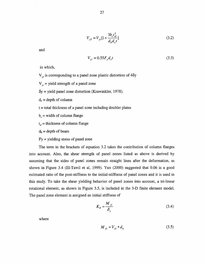
27
and
in which,
V y2 is corresponding to a panel zone plastic distortion of 4by
V yl = yield strength of a panel zone
by = yield panel zone distortion (Krawinkler, 1978).
de = depth of column
t = total thickness of a panel zone including doubler plates
be = width of column flange
tef = thickness of column flange
db = depth of beam
Fy = yielding stress of panel zone
(3.2)
(3.3)
The term in the brackets of equation 3.2 takes the contribution of column flanges
into account. Also, the shear strength of panel zones listed as above is derived by
assuming that the sides of panel zones remain straight lines after the deformation, as
shown in Figure 3.4 (EI-Tawil et aI, 1999). Yun (2000) suggested that 0.06 is a good
estimated ratio of the post-stiffness to the initial-stiffness of panel zones and it is used in
this study. To take the shear yielding behavior of panel zones into account, a tri-linear
rotational element, as shown in Figure 3.5, is included in the 3-D finite element model.
The panel zone element is assigned an initial stiffness of
(3.4)
where
(3.5)
28
F 8 =-y-
y .J3G (3.6)
where,
G = the shear modulus
3.6 Modeling of Nonlinearity
This study considers both material and geometric nonlinearity. Material
nonlinearity refers to the nonlinear relationship between the stresses and strains in an
element, and thus depends on the constitutive properties of the material. To take the
nonlinear deformation of columns of moment frames into account, the perfect elastic
plastic stress-strain curve as shown in Figure 3.6 is used to reproduce the material
nonlinearity of columns. In addition, the Bouc-W en model is used to simulate the
hysteretic response of beam-column connection. Geometric nonlinearity, on the other
hand, is a result of large displacements or rotations. Wang (2000) developed a 3-d finite
element program, in which the p-~ effect is included. However, the formulation of
elements was not based on the deformed shape in the step-by-step integration.
Consequently, geometric nonlinearity was ignored in the element calculations. To capture
the p-~ effect and the geometric nonlinearity in this study, a large displacement analysis
is performed, in which elements are formulated in the current configuration using current
nodal positions.
3.7 Modeling of Uncertainty
Structural reliability can be determined in terms of displacement demand versus
displacement capacity. In this study, the maximum column drift ratio (MCDR) is used to
measure both the demand and the capacity. Since the uncertainty in displacement demand
and displacement capacity may be due to the inherent variability (aleatory) uncertainty
and/or the modeling error (epistemic) uncertainty, both uncertainties will be considered.

29
The displacement demand (D d ) is determined by performing a suite of time history
analyses of the response under the SAC ground motions. The displacement capacity (Dc)
is determined by performing Incremental Dynamic Analysis (Vamvatsikos and Cornell,
2002).
Figure 3.7 shows an example of the results of demand analyses for a building.
Points labeled with D represent the response of a single structure under different SAC
ground motion excitations. Points labeled with 0 represent the median response at each
of the two probability levels. Solid line includes the correction for modeling error using
the correction factor following Wen and Foutch (1997). The displacement demand (Dd )
is represented by the corrected median response, as shown on the solid line, Figure 3.7.
The connection capacity against rotation is modeled as a normal random variable
with mean and standard deviation given by those in FEMA 355D. The yield strength and
the elastic modulus are also assumed to follow a normal distribution based on previous
experimental results. These parameters will be generated via the Monte-Carlo method.
Figure 3.8 shows an example of the capacity of a building against incipient collapse.
This capacity is random and difficult to predict, particularly when the structural response
goes into a nonlinear range. The Incremental Dynamic Analysis (IDA) is used for this
purpose.
Details of the uncertainty treatment are described in the following sections.
3.7.1 Modeling of Ground Motions
SAC phase-2 ground motions (Somerville, 1997) corresponding to 2% and 10%
exceedance probability in 50 years are used in this study. They are recorded and
simulated accordance with the USGS uniform-hazard target response spectra. Examples
of SAC phase-2 time history ground motions are shown in Figure 3.9, and the elastic
spectral acceleration with 5% damping of these ground motions are shown in Figure 3.10.
Structural time history response is calculated for each of ten uniform-hazard ground
motions. The advantage of using such ground motions is that the suite of ten ground
30
motions allows evaluation of the structural response of small probability of exceedance
that normally required a considerably larger number (thousands) of structural response
analyses.
3.7.2 Monte-Carlo Simulation in Materials and Member Properties
Material properties of buildings and the capacity of connections are inherently
random and need to be considered in the structure redundancy analyses. In view of the
complexity and uncertainty of the nonlinear structure response, a probabilistic treatment
is necessary and can be executed via Monte-Carlo simulations. Normal distributions are
used to model the uncertainty in the material properties and connections. The yield
strength of Grade 50 steel (FY) and elastic modulus of structural members are modeled
by normal variables with mean values equal to 50 (ksi) and 29000 (ksi), and a coefficient
of variation of 15% and 4%, respectively (Kennedy and Baker, 1984). The connection
capacity against rotation is also modeled as a normal random variable with parameters
following those in FEMA 355D, and details are described in Chapter 2.
3.7.3 Incremental Dynamic Analysis
System capacity against incipient collapse is determined by the incremental
dynamic analysis (IDA) (Vamvatsikos and Cornell, 2002). A single-record IDA is a
series of dynamic nonlinear analyses of one building under a single ground motion scaled
incrementally in terms of its elastic spectral acceleration. The result is highly dependent
on the record chosen; therefore, to capture the uncertainty, it is necessary to perform IDA
analyses of the same building under different ground motions.
The capacity described by each IDA curve, in terms of the drift ratio, is taken at the
point when the curve slope is less than 20% of the initial slope (Vamvatsikos and Cornell,
2002). The displacement capacity is assumed to follow a log-normal distribution. IDA is
extended to 3-D analyses, in which the aleatory uncertainty in ground motions,
connections and material properties are considered as described in foregoing sections,
31
from which the system capacity against incipient collapse and uncertainty can be
determined.
3.7.4 Uncertainty Correction Factor for Modeling Errors
To include epistemic uncertainties (modeling errors) in the structural demand
analysis, a correction factor is applied to the median response (Wen and Foutch, 1997).
The correction factor is given by
in which
1 ~2 CF =1+-Suy 2
(3.7)
(3.8)
(3.9)
(3.10)
S stands for a sensitivity factor; A and ~ are the log-normal distribution parameters
in the elastic spectral acceleration hazard curve; Sam is the median system limit state
capacity in terms of elastic spectral acceleration; Y is the total uncertainty random
variable assumed to be log-normal; (iy is the coefficient of variation of Y, related to the
variance of InY by equation 3.9; O"l!Y can be obtained by combining the record-to-record
response variation for a given elastic spectral acceleration, O"l! Dis' and the capacity
modeling errors'O"l!D . O"~D is assumed to be 30% in this study (Yun, Hamburger and cao cap
Cornell et aI, 2002).
32
3.8 Building Design
Buildings are designed according to the current code and the connection capacities
against rotation are randomized as described in Chapter 2. Both pre-Northridge and post
Northridge connections are considered in the moment frames.
3.8.1 Design Assumptions
The design of the moment frame follows the 2000 International Building Code and
the 1997 AISC Seismic Provisions. Design assumptions for special moment resisting
frames are:
1. Strong column weak beam (SCWB) guideline is used, i.e. the sum of the
moments in the column above and below the joint at the intersection of beam and column
centerlines should be no less than the sum of the moments in the beams at the intersection
of beam and column centerlines.
2.5% damping in first and second modes is used in the time history analysis.
3. The floors are modeled as flexible diaphragms. The SCWB design guideline is
used to prevent plastic hinges in the columns. Notice that, a rigid diaphragm can cause
plastic hinges in the columns. In addition, to consider the effects of fracture of
beam/column connections, beams and floors should remain flexible to allow the
development of such fracture failures.
4. 5% accidental torsional moment produced by horizontal offset in the center of
mass is assumed.
5. The buildings are located in Los Angeles, California. The site class is assumed to
be type D. Seismic Use Group I is assigned to the bUilding. For example, the seismic
response coefficient (Cs) could be calculated by the follows:
C = SDL
s (~I*T IE )
(3.11)
33
in which SDL is the design spectral acceleration, R (= 8) is the response modification
factor, IE (= 1) is the occupancy importance factor, and T is the fundamental period
estimated by 0.035x(H)o.75. H is the height of building (ft).
In most cases, the assumptions above lead to beam sizes controlled by the strength
requirement instead of the drift criteria, and the column sizes are controlled by the SCWB
guideline.
3.8.2 Design Results
Nine different designs are obtained for each of the 3-story and 12-story buildings.
Buildings are square in plan configuration with width and length of 150 ft. The story
height is 13 feet. There are five bays in each direction. The plan configuration, number
and arrangement of moment frame follow those prototype designs in the recent proposal
submitted to NEHRP (NEHRP Proposal 2-1 R), which has been adopted in NEHRP 2003.
These designs are used in this study because they are designed and proposed by engineers,
and are believed to be commonly used in this country. They also allow a direct
comparison of the redundancy factors proposed in NEHRP 2003 and the uniform-risk
redundancy factor proposed in this study. The plan configurations of these nine different
buildings are displayed in Figure 3.11, in which the abbreviations of buildings are used in
these figures and throughout this paper. They are explained as follows:
1. 3 _s_3bay _3bay: 3-story building with three moment bays in both directions.
Only the three center bays of the perimeter frames are designed as moment
frames. The rest are gravity frames.
2. 3_s_2bay_2bay: 3-story building with two moment bays in both directions.
Only the two center bays of the perimeter frames are designed as moment
frames. The rest are gravity frames.
3. 3_s_1bay_1bay: 3-story building with one moment bay in both directions. Only
the center bay of the perimeter frames is designed as a moment frame. The rest
are gravity frames.
34
4. 3_s_3bay_1bay: 3-story building with three moment bays in N-S direction and
one moment bay in E-W direction. Only the three center bays of the perimeter
frames (N-S direction) and the center bay of the perimeter frame (E-W
direction) are designed as moment frames. The rest are gravity frames.
5. 3_s_2bay_1bay: 3-story building with two moment bays in N-S direction and
one moment bay in E-W direction. Only the two center bays of the perimeter
frames (N-S direction) and the center bay of the perimeter frame (E-W
direction) are designed as moment frames. The rest are gravity frames.
6. 3_s_3bay _1 bay_interior: 3-story building with three moment bays in N-S
direction, and one moment bay in the core area. The three center bays of the
perimeter frames in the N-S direction and the center bay in the core area (E-W
direction) are designed as moment frames. The rest are gravity frames.
7. 3_s_2bay_1bay_interior: 3-story building with two moment bays in N-S
direction, and one moment bay in the core area. The two center bays of the
perimeter frames in the N -S direction and the center bay in the core area (E-W
direction) are designed as moment frames. The rest are gravity frames.
8. 3_s_1bay_1bay_interior: 3-story building with one moment bay in N-S
direction, and one moment bay in the core area. The center bay of the perimeter
frames in the N-S direction and the center bay in the core area (E-W direction)
are designed as moment frames. The rest are gravity frames.
9. 3_s_1 bay_interior_1 bay_interior: 3-story building with one moment bay in
both directions. Only the center bay of the core area in both directions is
designed as moment frames. The rest are gravity frames.
The abbreviations of 12-story buildings follow those of 3-story buildings. Table 3.1
and Table 3.2 show the design details of moment frames of 3-story buildings and 12-
story buildings, respectively. Table 3.3 and Table 3.4 show the design details of gravity
frames of 3-story and 12-story buildings, respectively. Table 3.5 describes periods of
each of 3-story and 12-story buildings. Table 3.6 provides the information of dimensions
and properties of plate girders, which are used in the designs of 12-story buildings. Figure

35
3.12 and Figure 3.13 display the finite element model of 3-story and 12-story building,
respectively, where the bold lines represent the moment frames.
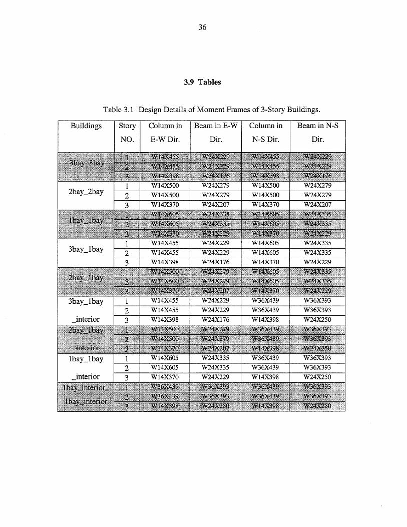
Buildings
36
3.9 Tables
Table 3.1 Design Details of Moment Frames of 3-Story Buildings.
Story Column in Beam in E-W Column in
NO. E-W Dir. Dir. N-S Dir.
Beam in N-S
Dir.
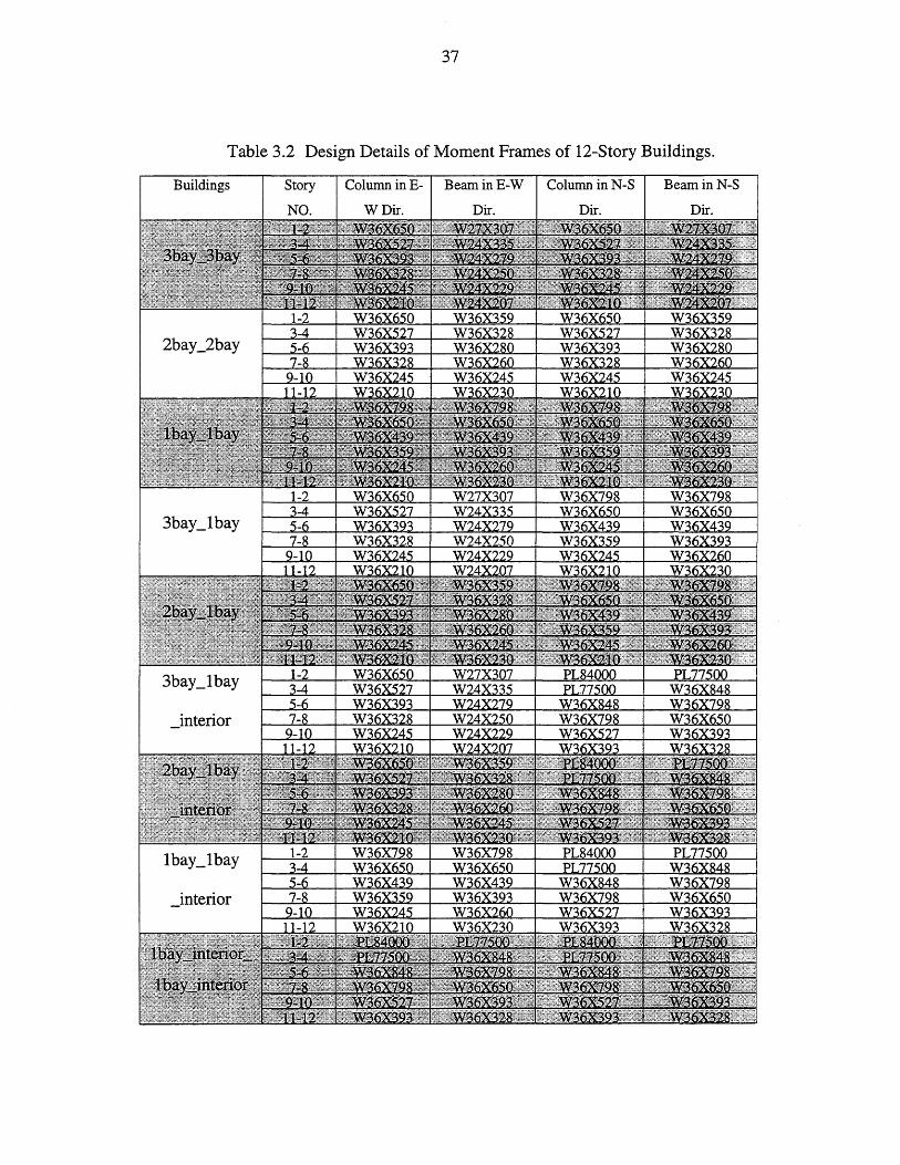
37
Table 3.2 Design Details of Moment Frames of 12-Story Buildings.
Buildings Story
NO.
Column in E- Beam in E-W Column in N-S
W Dir. Dir. Dir.
BeaminN-S
Dir.
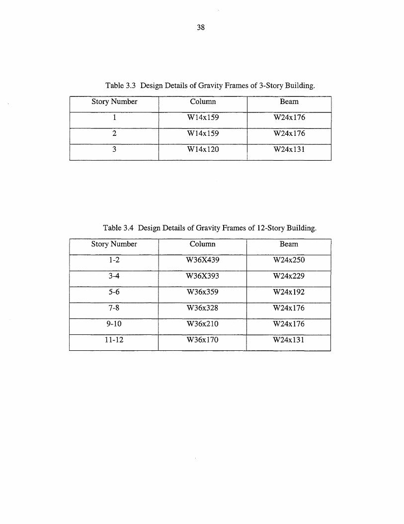
38
Table 3.3 Design Details of Gravity Frames of 3-Story Building.
Story Number Column Beam
1 W14x159 W24x176
2 W14x159 W24x176
3 W14x120 W24x131
Table 3.4 Design Details of Gravity Frames of 12-Story Building.
Story Number Column Beam
1-2 W36X439 W24x250
3-4 W36X393 W24x229
5-6 W36x359 W24x192
7-8 W36x328 W24x176
9-10 W36x210 W24x176
11-12 W36x170 W24x131
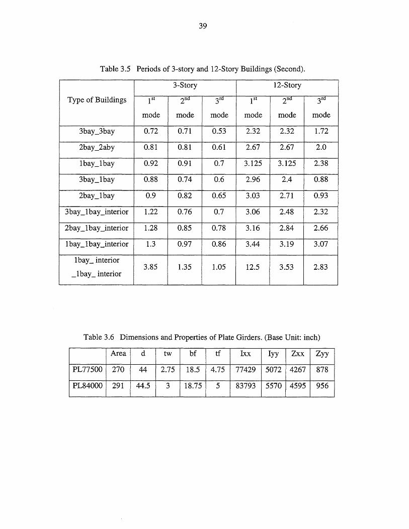
39
Table 3.5 Periods of 3-story and 12-Story Buildings (Second).
3-Story 12-Story
Type of Buildings 1 st 2nd 3rd 1 st 2nd 3rd
mode mode mode mode mode mode
3bay_3bay 0.72 0.71 0.53 2.32 2.32 1.72
2bay_2aby 0.81 0.81 0.61 2.67 2.67 2.0
1bay_1bay 0.92 0.91 0.7 3.125 3.125 2.38
3bay_1bay 0.88 0.74 0.6 2.96 2.4 0.88
2bay_1bay 0.9 0.82 0.65 3.03 2.71 0.93
3bay _1 bay_interior 1.22 0.76 0.7 3.06 2.48 2.32
2bay _1 bay_interior 1.28 0.85 0.78 3.16 2.84 2.66
1 bay _1 bay_interior 1.3 0.97 0.86 3.44 3.19 3.07
1 bay_ interior 3.85 1.35 1.05 12.5 3.53 2.83
_1bay_ interior
Table 3.6 Dimensions and Properties of Plate Girders. (Base Unit: inch)
Area d tw bf tf Ixx Iyy Zxx Zyy
PL77500 270 44 2.75 18.5 4.75 77429 5072 4267 878
PL84000 291 44.5 3 18.75 5 83793 5570 4595 956
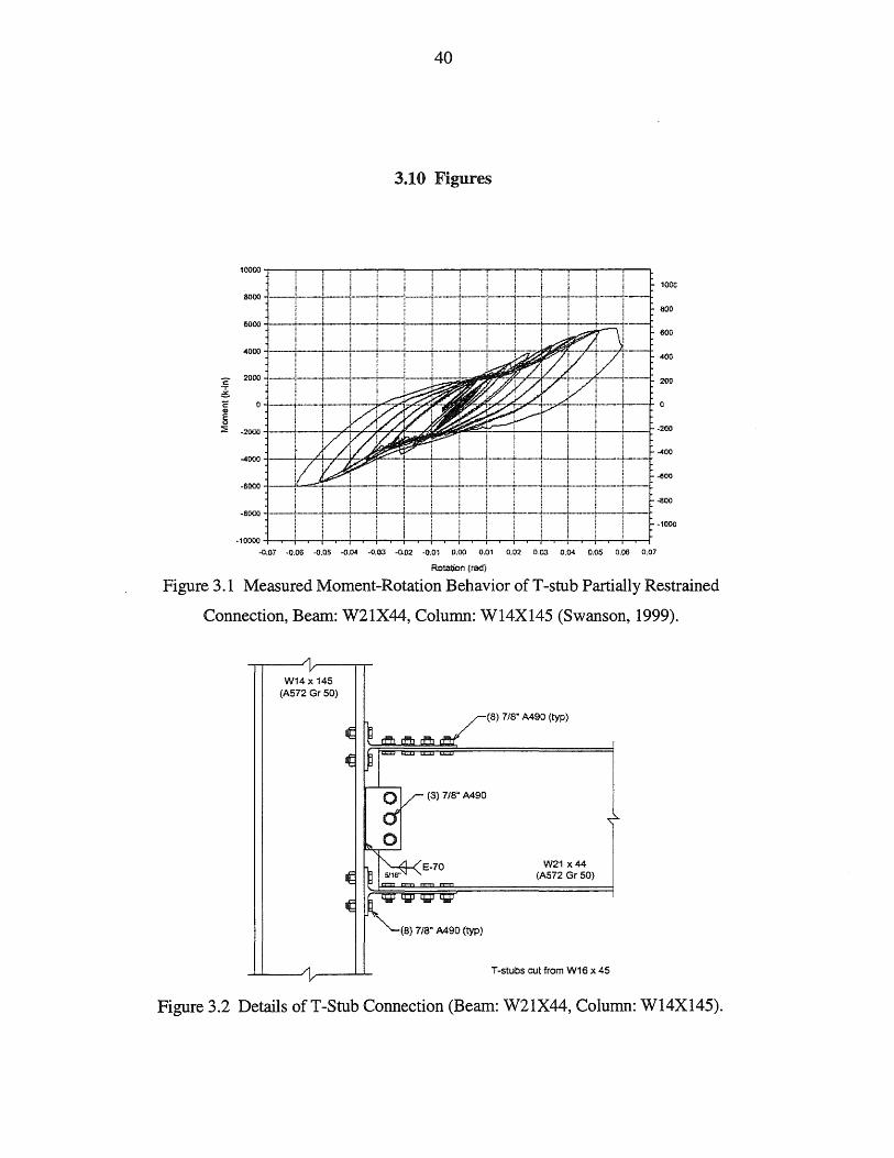
40
3.10 Figures
10000 .,.---.---.---.--..,----.---..,----.---.---.---.---.---..,----.---L I f I I I • I !
:~! i t- ! t+tt= i 1-1 : !=t-1000
~QO
600 J t ! I ! f ! i !'
4000 __ 1 __ - ..... 1 __ L __ I --.. L. __ .L._ .. __ ...L __ .. i ____ ~-_. I
iii ! ! i I t I 400 I i I I:! f
C 2000 __ ·I ___ + __ -+_+_+ __ ~----L. '
~ 0 --J--L--l-I . . i '!! ! :E -2Q(J(j i :;~~~ii'~fiP.!-~-I;::.--=---I--~
¥-... ~"--1---~--~--I-·-·-~-_+--!-----t---~---
200
·200
-400
j I Ii: ._. __ 1 ___ , _--.J ___ L __ ..L ___ J ___ -1 .. ___ 1 .. ___ -l_ ... ____ L ___ .. ..: __
I I I I ! I ! I I ! I I ---!._ .. _--i---+--.--! ----i---4-.---4--·--! .. ·---·-+--.. --i...--+--... ---.. +.----!---
i ; ! ! !! I!!! i !
-6000
-BOOO
~oo
-aClO
·1000
.. 10000 -1-....--+
'
--r-+--r-+l--r-+~ --r-+--r-+--r-+--r-+I--r-+--r-+I--r-+J --r-+i --r--+! --.--1 -O.Oi ·0.06 -{I.OS -0.0<1 ·0.03 -0.02 -0.01 0.00 0.01 0.02 C.O;! O.C4 0.05 0.00 0.07
Rotation (rad)
Figure 3.1 Measured Moment-Rotation Behavior ofT-stub Partially Restrained
Connection, Beam: W21X44, Column: W14X145 (Swanson, 1999).
W14x 145 (A572 Gr 50)
{8} 7/8* A490 (typ)
(8) 7/8" A490 (typ)
W21 x44 (A572 Gr 50)
T-stubs cut from W16 x 45
Figure 3.2 Details ofT-Stub Connection (Beam: W21X44, Column: W14X145).
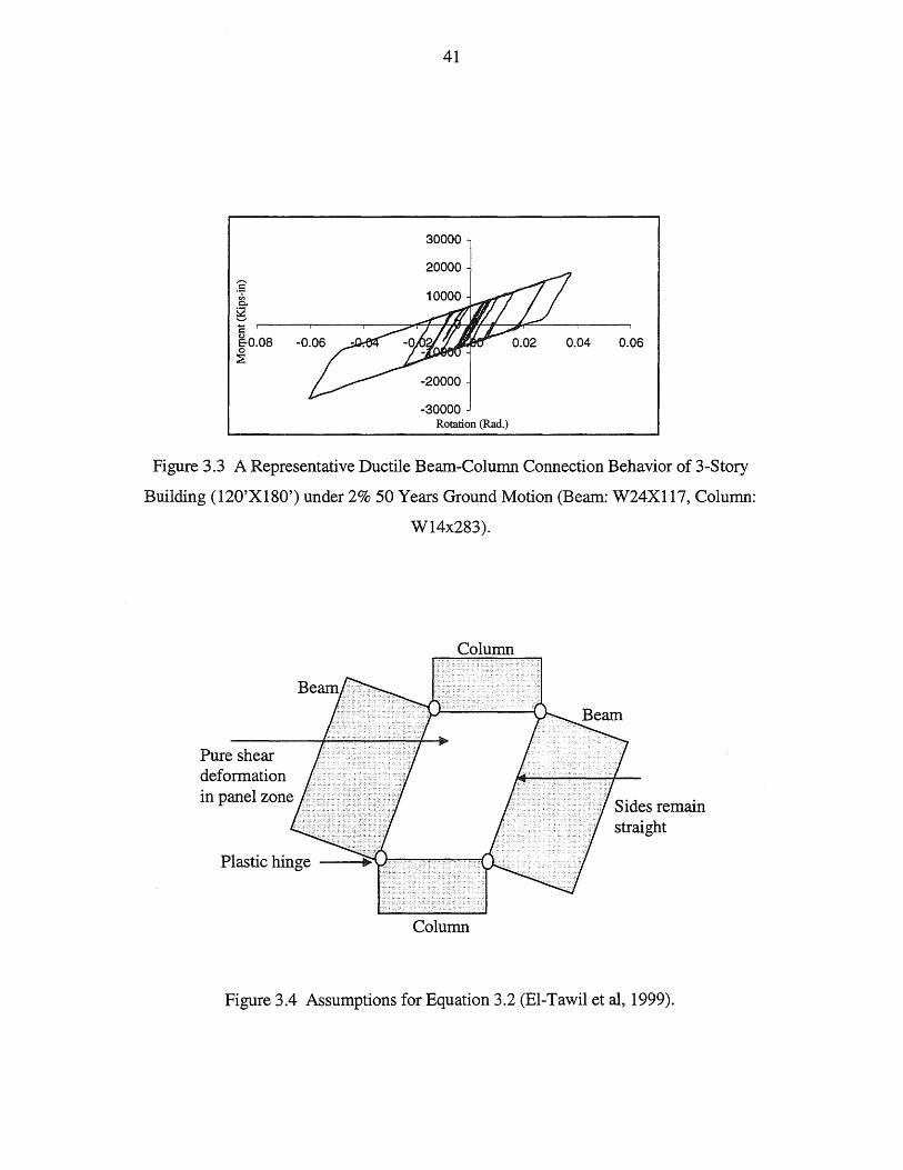
= &0.08 o
:::E
41
30000
0.06
-30000 Rotation (Rad.)
Figure 3.3 A Representative Ductile Beam-Column Connection Behavior of 3-Story
Building (120'X180') under 2% 50 Years Ground Motion (Beam: W24Xl17, Column:
Pure shear deformation in panel zone
Plastic hinge --..-
W14x283).
Column
Column
Sides remain straight
Figure 3.4 Assumptions for Equation 3.2 (EI-Tawil et aI, 1999).
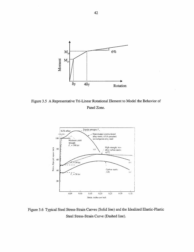
42
...... M _ .....
J yl I
~~------~------------------~ oy 40y Rotation
Figure 3.5 A Representative Tri-Linear Rotational Element to Model the Behavior of
Panel Zone.
I.f)(! I
!
]
'" ~ or.
~
f ::;:: 40
20
Minimum 11dii ~tre!1:lth F, :::~W(}k:>i
OJO
/r" Hell.t··tri:~ted <::<:;n~1.111ctiol1:;11 .... :llloy ~tt'.eb: AS 14 I.juench~d
and tcmpcr~~ ;J\!()Y sled
HiglH;treng!h. to~\". ;litO), ,:arbon ;.1eeb: /\572
(US 0.·.20 O.3f)
$tr.lin.im:llt's ly<:r inch
Figure 3.6 Typical Steel Stress-Strain Curves (Solid line) and the Idealized Elastic-Plastic
Steel Stress-Strain Curve (Dashed line).
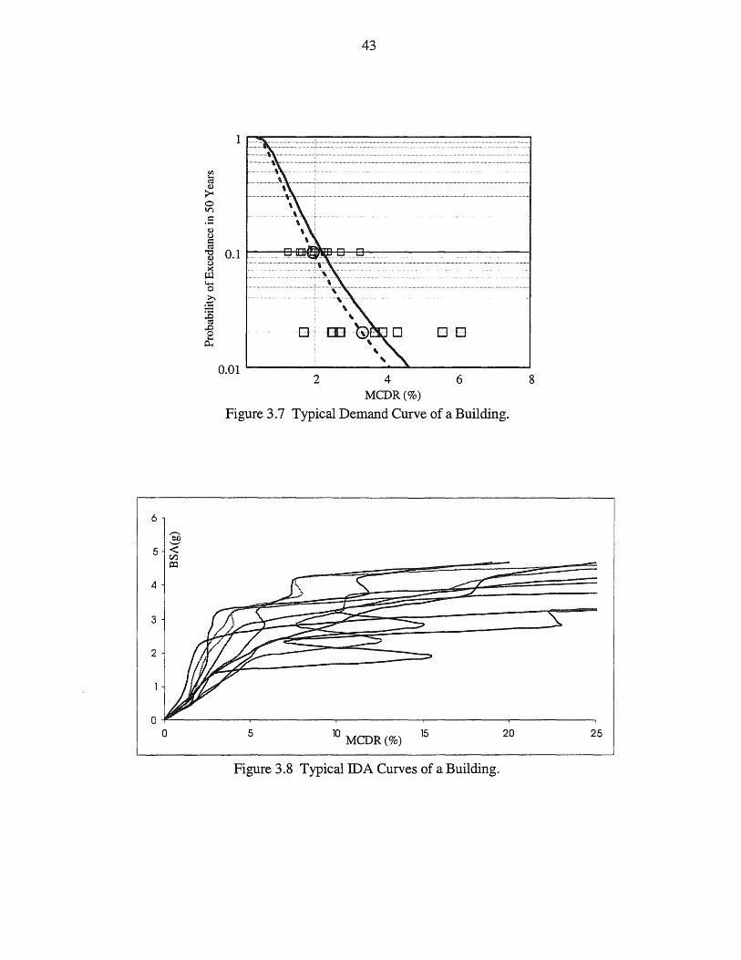
43
1
CJJ a Q)
~ 0 III
.5 Q) u = C';S
"0 0.1 Q) u ><: ~ 4-4 0
g :§ ..0 0 0 0 '"" ~
0.01 2 4 6 8
MCDR(%)
Figure 3.7 Typical Demand Curve of a Building.
6
4
3
2
5 10 MCDR(%) 15 20 25
Figure 3.8 Typical IDA Curves of a Building.
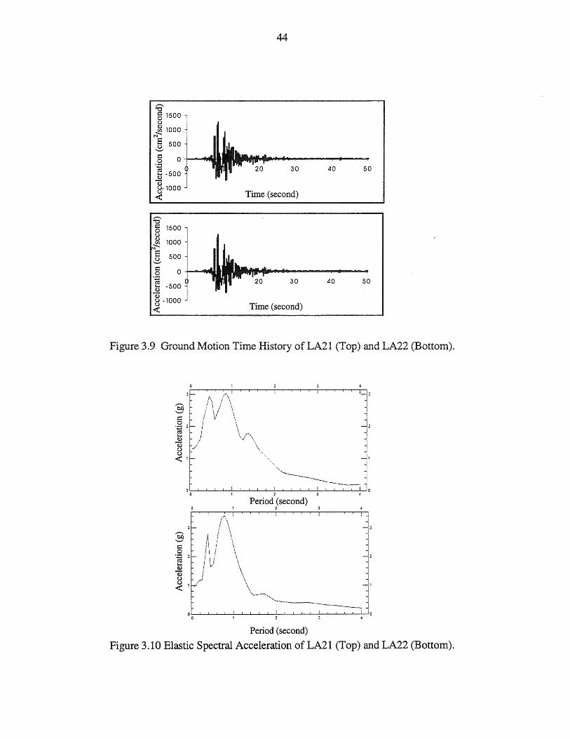
44
-"0 § 1500 u ~ 1000
N e 500 u "-' t:: 0 0 .~ 30 40 50 ~ -500 ~ ~-1000
Time (second) <
-"0 t:: 1500 0 u Q)
1000 en -.. e 500 u "-' t:: 0 0 .~
-500 30 40 50
~ Q)
~ ~ -1000
Time (second) <
Figure 3.9 Ground 1\1otion Time History of LA21 (Top) and LA22 (Bottom).
'-.._-_._._.---_ .. _-_._ ... _. 2
Period (second) 2
/'. I
! \ f \
I~ i \ Ji i \ !\ i \
I I
31-
I V \ i \
1-:,/) \ \ '_ ................... ,
' ........ -._--_. '-"-"-'~-
-3
-2
-1
O~~~~_I~~~_L_~I,~~~_L_I~~~~I o
Period (second)
Figure 3.10 Elastic Spectral Acceleration ofLA21 (Top) and LA22 (Bottom).

r
45
1 bay _interior_1 bay
_interior
Figure 3.11 Nine Plan Configurations of 3-Story and 12-Story Buildings (Bold Lines
Represent the Moment Frames).
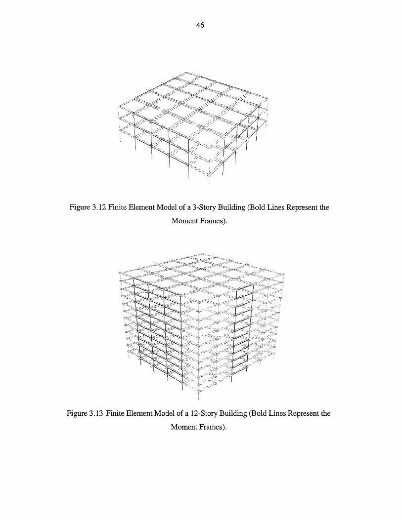
46
Figure 3.12 Finite Element Model of a 3-Story Building (Bold Lines Represent the
Moment Frames).
Figure 3.13 Finite Element Model of a 12-Story Building (Bold Lines Represent the
Moment Frames).
47
CHAPTER 4 STRUTURAL RESPONSE, DEMAND AND CAPACITY ANAL YSES
4.1 Introduction
Most structures exhibit nonlinear behavior under severe seismic excitations. The
structural response becomes more complicated and the principle of superposition is no
longer valid. Research has shown that the random vibration of nonlinear structures is
generally difficult. The Monte-Carlo simulation, on the other hand, has been well
developed and becomes more efficient as computation speed increases with time. As
there is significant uncertainty in three-dimensional structures under dynamic stochastic
loads such as earthquakes and the complicated restoring force behavior exists due to
brittle connection failure, simulation techniques and time history analyses may be the
most appropriate methods for evaluating a nonlinear system. Therefore, in this study the
Monte-Carlo simulation method is used for nonlinear response analysis and evaluation of
structural performance, structural reliability and redundancy.
Nine 3-story and 12-story buildings of different configurations described in section
3.8.2 are studied in section 4.2 to section 4.9. Four other bUildings, designed to
investigate the effects of floor area, are studied in section 4.10.
4.2 Responses Analyses of 3- and 12-Story Buildings
A modal analysis is performed for each of 3- and 12-story buildings with nine
different configurations, described in section 3.8.2, and the structural period and mode
shapes are obtained. With this information, an appropriate design and the modeling of a
building are ensured. Dynamic time history analysis is performed for each building as
well, and the following important factors are considered: (1) uncertainties in material
properties; (2) uncertainties in connection capacity; (3) effects of gravity frames; (4) p-~
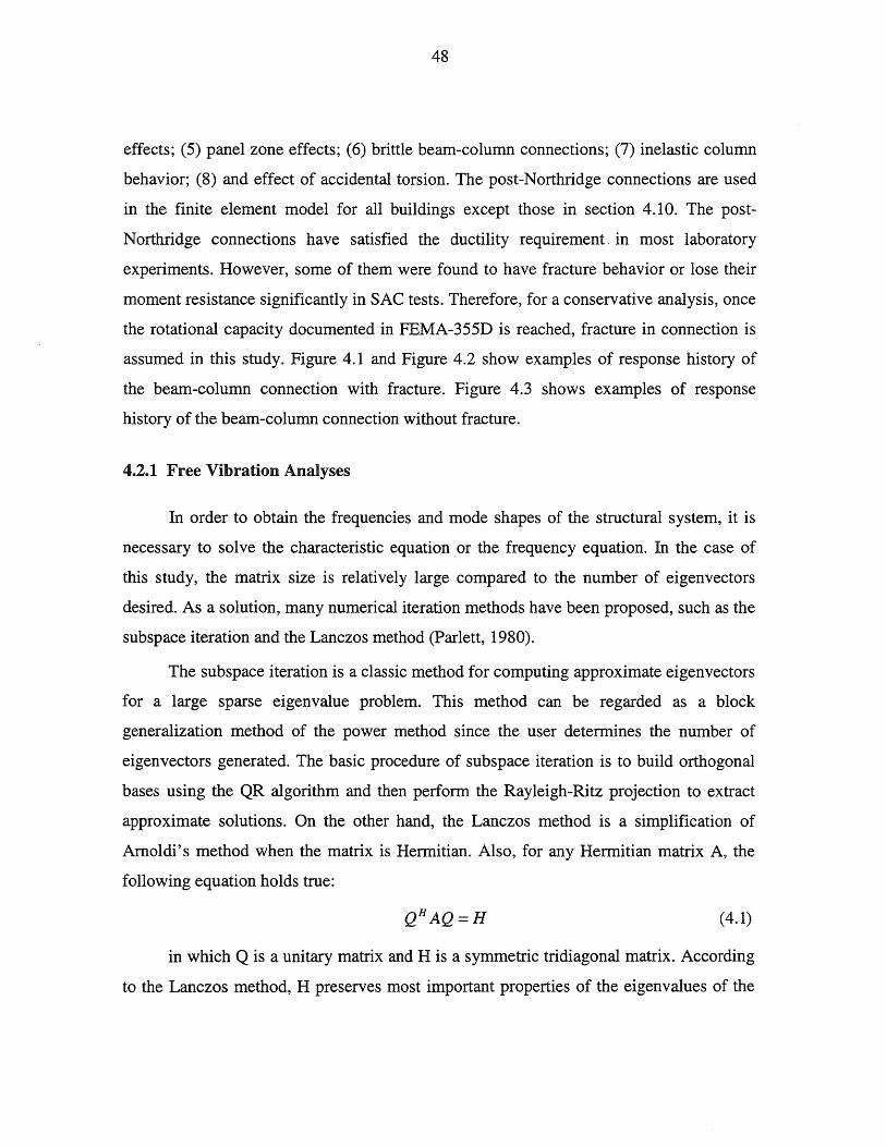
48
effects; (5) panel zone effects; (6) brittle beam-column connections; (7) inelastic column
behavior; (8) and effect of accidental torsion. The post-Northridge connections are used
in the finite element model for all buildings except those in section 4.10. The post
Northridge connections have satisfied the ductility requirement. in most laboratory
experiments. However, some of them were found to have fracture behavior or lose their
moment resistance significantly in SAC tests. Therefore, for a conservative analysis, once
the rotational capacity documented in FEMA-355D is reached, fracture in connection is
assumed in this study. Figure 4.1 and Figure 4.2 show examples of response history of
the beam-column connection with fracture. Figure 4.3 shows examples of response
history of the beam-column connection without fracture.
4.2.1 Free Vibration Analyses
In order to obtain the frequencies and mode shapes of the structural system, it is
necessary to solve the characteristic equation or the frequency equation. In the case of
this study, the matrix size is relatively large compared to the number of eigenvectors
desired. As a solution, many numerical iteration methods have been proposed, such as the
subspace iteration and the Lanczos method (Parlett, 1980).
The subspace iteration is a classic method for computing approximate eigenvectors
for a large sparse eigenvalue problem. This method can be regarded as a block
generalization method of the power method since the user determines the number of
eigenvectors generated. The basic procedure of subspace iteration is to build orthogonal
bases using the QR algorithm and then perform the Rayleigh-Ritz projection to extract
approximate solutions. On the other hand, the Lanczos method is a simplification of
Arnoldi's method when the matrix is Hermitian. Also, for any Hermitian matrix A, the
following equation holds true:
(4.1)
in which Q is a unitary matrix and H is a symmetric tridiagonal matrix. According
to the Lanczos method, H preserves most important properties of the eigenvalues of the

49
original matrix A. Using the Lanczos method to create the H matrix and Q matrix, which
consists of the number of vectors referred to as Lanczos vectors, enables finding
eigenvalues of matrix H without computational difficulty. Parlett (1980) and Saad (1992)
discuss the details of subspace iteration and the Lanczos method. Implementations of the
subspace iteration and the Lanczos method are both available in ABAQUS. This study
uses the subspace iteration to compute frequencies (eigenvalues) and mode shapes
(eigenvectors).
Table 3.5 displays the periods of all 3-story buildings. The range of fundamental
period is from 0.72 second and 1.3 second (exclude the 1bay_interior_1bay_interior
case). Yun (2000) did an analysis of the period of buildings based on measured data from
a report by Goel and Chopra (1997). According to Yun's regression result, the median
period of 3-story buildings is 0.7 second. The calculated values from this study are a little
higher than that from Yun's regression analysis; nevertheless, they are within a
reasonable range. It is important to emphasize that the 3_s_1bay_interior_1bay_interior
building has a longer fundamental period than those of other buildings, due to the poor
plan configuration design as demonstrated in Figure 3.11. Consequently, torsion will
dominate the building response when moment frames are located only in the core area of
a building. As a result, the first mode of this building is rotational instead of translational
(X or Y direction). Figure 4.4 shows the first three mode shapes of the 3bay_3bay
building; it is also true for other buildings except 1 bay _interior_1 bay_interior building.
Figure 4.5 shows the first three mode shapes of the 1 bay _interior_1 bay_interior building:
rotation dominates the overall response.
Table 3.5 displays the periods of all 12-story buildings. The range of the
fundamental period is from 2.32 second and 3.44 second excluding the
1bay_interior_1bay_interior case. Based on Yun's regression results (2000), the median
period of 12-story is 2.1 second. The calculation values from this study are again a
slightly higher than the results of the regression analysis. The
12_s_1 bay _interior_1 bay_interior building has a longer fundamental period than other
buildings, as the case of the 3-story buildings, indicating again that a poor design may
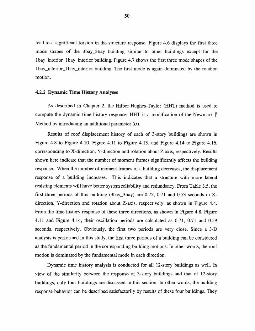
50
lead to a significant torsion in the structure response. Figure 4.6 displays the first three
mode shapes of the 3bay_3bay building similar to other buildings except for the
1bay_interior_1bay_interior building. Figure 4.7 shows the first three mode shapes of the
1bay_interior_1bay_interior building. The first mode is again dominated by the rotation
motion.
4.2.2 Dynamic Time History Analyses
As described in Chapter 2, the Hilber-Hughes-Taylor (HHT) method is used to
compute the dynamic time history response. HHT is a modification of the Newmark ~
Method by introducing an additional parameter (a.).
Results of roof displacement history of each of 3-story buildings are shown in
Figure 4.8 to Figure 4.10, Figure 4.11 to Figure 4.13, and Figure 4.14 to Figure 4.16,
corresponding to X-direction, Y-direction and rotation about Z axis, respectively. Results
shown here indicate that the number of moment frames significantly affects the building
response. When the number of moment frames of a building decreases, the displacement
response of a building increases. This indicates that a structure with more lateral
resisting elements will have better system reliability and redundancy. From Table 3.5, the
first three periods of this building (3bay_3bay) are 0.72, 0.71 and 0.53 seconds in X
direction, Y-direction and rotation about Z-axis, respectively, as shown in Figure 4.4.
From the time history response of these three directions, as shown in Figure 4.8, Figure
4.11 and Figure 4.14, their oscillation periods are calculated as 0.71, 0.71 and 0.59
seconds, respectively. Obviously, the first two periods are very close. Since a 3-D
analysis is performed in this study, the first three periods of a building can be considered
as the fundamental period in the corresponding building motions. In other words, the roof
motion is dominated by the fundamental mode in each direction.
Dynamic time history analysis is conducted for all 12-story buildings as well. In
view of the similarity between the response of 3-story buildings and that of 12-story
buildings, only four buildings are discussed in this section. In other words, the building
response behavior can be described satisfactorily by results of these four buildings. They
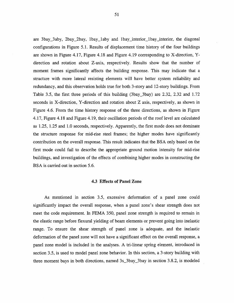
51
are 3bay_3aby, 2bay_2bay, 1bay_1aby and 1 bay_interior_1 bay_interior, the diagonal
configurations in Figure 5.1. Results of displacement time history of the four buildings
are shown in Figure 4.17, Figure 4.18 and Figure 4.19 corresponding to X-direction, Y
direction and rotation about Z-axis, respectively. Results show that the number of
moment frames significantly affects the building response. This may indicate that a
structure with more lateral resisting elements will have better system reliability and
redundancy, and this observation holds true for both 3-story and 12-story buildings. From
Table 3.5, the first three periods of this building (3bay_3bay) are 2.32, 2.32 and 1.72
seconds in X-direction, Y-direction and rotation about Z axis, respectively, as shown in
Figure 4.6. From the time history response of the three directions, as shown in Figure
4.17, Figure 4.18 and Figure 4.19, their oscillation periods of the roof level are calculated
as 1.25, 1.25 and 1.0 seconds, respectively. Apparently, the first mode does not dominate
the structure response for mid-rise steel frames; the higher modes have significantly
contribution on the overall response. This result indicates that the BSA only based on the
first mode could fail to describe the appropriate ground motion intensity for mid-rise
buildings, and investigation of the effects of combining higher modes in constructing the
BSA is carried out in section 5.6.
4.3 Effects of Panel Zone
As mentioned in section 3.5, excessive deformation of a panel zone could
significantly impact the overall response, when a panel zone's shear strength does not
meet the code requirement. In FEMA 350, panel zone strength is required to remain in
the elastic range before flexural yielding of beam elements or prevent going into inelastic
range. To ensure the shear strength of panel zone is adequate, and the inelastic
deformation of the panel zone will not have a significant effect on the overall response, a
panel zone model is included in the analyses. A tri-linear spring element, introduced in
section 3.5, is used to model panel zone behavior. In this section, a 3-story building with
three moment bays in both directions, named 3s_3bay_3bay in section 3.8.2, is modeled
52
with and without panel zone elements to investigate the influence of panel zones on the
global response. The building is subjected to a pair of SAC phase 2 ground motions,
LA31 and LA32 corresponding to the probability level of 2% in 50 years. Figure 4.20
shows the time history of building roof response with and without considering panel zone
effects. The peak responses of two buildings are not much difference except the rotational
motion. However, the magnitude of the rotation is relatively small, and its effect on the
overall response can be ignored. The maximum column drift ratios in two cases are
shown in Figure 4.21. The MCDR of a building with panel zone modeling is slightly
larger than that of a building without panel zone, i.e. 4.7 to 4.3. Figure 4.22 shows the
response time history of the panel zone - one within elastic range, the other just into
inelastic range. Given that the development of panel zone inelastic deformation is not
remarkable, results shown here indicate that panel zones only have a moderate influence
on the overall response when its shear strength is adequate.
4.4 Comparisons of pre-Northridge and post-Northridge Connections
A commonly accepted practice in seismic designs is to take advantage of the
ductility capacity of the system. A ductile system can resist intense ground excitation
without collapse. Before the Northridge earthquake, the standard connections of steel
moment frames were thought to have ductility capability. After the earthquake, many
brittle connection failures were discovered and such pre-Northridge connections are no
longer acceptable. This section aims to investigate the difference between pre- and post
Northridge connection on the overall response, and the system demand and capacity are
used as measures for evaluation. The drift demand at two probability levels, 2% and 10%
in 50 years, is determined by multiplying the median MCDR, determined from the time
history analyses, with the correction factors as described in section 3.7.4. The
displacement capacity (Dc) against incipient collapse is determined by performing IDA
as described in section 3.7.3. The structure, named 3s_3bay_3bay (section 3.8.2),
53
presented in Figure 3.11, is modeled with both types of connections to demonstrate the
process and results of this evaluation.
Table 4.1 and Figure 4.23 show the results of the demand analysis. As expected,
fracture failure of the pre-Northridge connections has a serious impact on the building
performance. For the 2% in 50 years hazard, the median drift demand of pre-Northridge
buildings is almost doubled compared to that of the post-Northridge buildings.
Figure 4.24 shows the results of IDA analysis. Building properties are randomized
as shown in section 2.3.2 and section 3.7. The incipient collapse capacity can be
determined from the IDA analysis and approximately described by a lognormal
distribution as shown in Figure 4.25. Table 4.2 shows the statistics of drift capacities for
the two buildings: the median capacity of the pre-Northridge building is only 80% of the
post -Northridge building.
4.5 Effects of Connection Fracture
This section aims to investigate the impacts of connection failures on the time
history analyses and the IDA. A 3-story building with three moment bays in E-W
direction and one moment bay in N-S direction (3bay_lbay) is used. The building is
modeled with or without connection fractures for comparison. The post-Northridge
connections as described in section 2.3.2 and section 4.2 are used. A pair of SAC phase 2
ground motions, LA 35 and LA 36 is used as the seismic excitations. As expected the
building with connection fractures have a serious impact on the structural response, as
shown in Figure 4.26. Also, the effective period of the building becomes longer as
fractures occurred. Moreover, the building with connection fracture will have a larger
permanent displacement compared to a building without connection fracture.
The structure, named 3s_3bay_3bay (section 3.8.2), shown in Figure 3.11, is used
for the evaluation of the IDA response. Figure 4.27 shows the ratio of fractured
connections to total connections in an IDA curve, in which the ground motions LA25 and
LA26 are used. The results indicate that the significant connection fractures start at about

54
BSA at 2.2g corresponding to the 2% in 50 years probability (2/50) level (nine of the
seventy-two connections are fractured). When the ground intensity increases to 1.4 times
2150 BSA, fifty-six of the seventy-two connections are fractured. At this point, the slope
of the IDA curve drops below the 20% of the initial slope, in other words, the structural
system is near the overall collapse stage. Results indicate that the connection fracture and
the overall stability are crucially interrelated and the connection failure significantly
impacts the overall performance.
4.6 Effects of Elastic-Plastic Column of Moment Frame
One of the design concepts of steel frames is to prevent the formulation of single
story mechanisms, in which plastic hinges form at both ends of all columns in a story. A
single-story mechanism can induce a large lateral displacement and thus lead to large
local drift demand and potential p-L\. instability. The Strong-Column-Weak-Beam
(SCWB) guideline is a common method for preventing a single-story mechanism. Still, it
is reasonable to question whether columns of SCWB frames will remain in the elastic
range under severe ground excitations.
To investigate the column response and its effect on structure performance, three
different modeling techniques are proposed: elastic column, elastic-plastic column and
lumped-plasticity column. Lumped-plasticity modeling is commonly used in a nonlinear
analysis because of its computational efficiency and its consistency with site
observations, in which column damage occurred in conjunction with weld damage or
beam fractures. In lumped-plasticity modeling, inelastic yielding of columns is assumed
to be confined to discrete hinge regions located at the ends of columns. Since the IDA is
used here to determine capacities of steel frames, intensity of excitation can be much
higher than that of any real earthquake. It is reasonable not to limit the development of
column plasticity to its boundary regions. Therefore, a column with elastic-plastic
material properties is also used to investigate the effects of column plasticity on the
overall response.
55
A 3-story building with three moment bays in both directions, named 3bay _3bay in
section 3.8.2, is modeled with the above three types of columns. Post-Northridge
connections are used in all cases. A pair of SAC phase 2 ground motions, LA 21 and LA
22 are used as the seismic excitations. Figure 4.28 shows the roof displacement of three
buildings, indicating that the elastic-plastic and lumped-plasticity model exhibits a
similar trend, and as expected, the response of the elastic-plastic model is slightly larger
than that of the lumped-plasticity model. Figure 4.29 shows an example of a nonlinear
response of a column, in which the column element is located at the base of a building,
and an elastic-plastic model is used. This result indicates that the use of SCWB does not
necessarily prevent plasticity development in columns.
4.7 Effects of Post-Fracture Behavior of Connections on MCDR Demand
In this section, effects of post-to-pre capacity ratio, rotational capacity of
connections and asymmetric post-fracture behavior will be discussed.
When the plastic rotation of connections reaches the capacity, 8p, the connection
will experience fracture or lose its moment resistance significantly (FEMA 355D). It is
difficult to determine how much residual moment capacity of connections will remain
since most tests will stop at this point. In the piecewise-linear model developed by Shi
(1997), the positive post-fracture moment ratio is assumed to be 30%, and the negative
post-fracture moment is assumed to be 50%. The post-fracture moment for both cases is
temporarily assumed to be 10% in this study. It is of interest to investigate the effects of
post-fracture moment of connections on MCDR demand on structures. Table 4.3 shows
the MCDR demand of 3bay_3bay and 1bay_1bay buildings with different post-fracture
moment ratios, in which the positive and negative post-fracture moment ratios are
assumed to be identical. Results indicate that the post-fracture moment capacity has only
slight influence on MCDR demand for 3bay _3bay building and for both buildings at the
hazard level of 10% in 50 years. This is because connections do not experience serious
fracture behavior due to redundancy (3bay _3bay) at the hazard level of 10% in 50 years.

56
On the other hand, at the hazard level of 2% in 50 years, the benefit of higher post
fracture moment ratio is more obvious for the Ibay_lbay building, but still moderate.
The rotational capacity, ep, has a significant influence on the structural response as
shown in the section 4.4 (the comparison of pre-Northridge and post-Northridge
connection), connection fracture will occur when ep is exceeded. Since it is dependent on
the depth of the beam, the sensitivity to the depth of beam becomes an important issue
and needs to be examined. Table 4.4 shows the relationship of 8p and the depth of beams
based on equation 2.20, which is used to model the random rotational capacity in this
study. The rotational capacity reduces to 0.038 from 0.043 when the depth of beam
increases from 24 inch to 40 inch. Since the beams used in this study are mostly within
this range, it may conclude that the depth of beam does not have significant effects on the
structural response.
Depending on the location of fracture (on the top, bottom or both); the post-fracture
hysteretic behavior could be asymmetric (Yang and Popov, 1995). Based on the results of
Table 4.3, in which the post fracture behavior is assumed to be symmetric, the MCDR
demand do not significantly depend on the post fracture moment ratio ranging from 10%
to 50%. It is reasonable to expect that the effects of unequal positive and negative post
fracture moment ratio within the same range (from 10% to 50%) will not be significant.
4.8 Performance Evaluation of 3 .. story Buildings
System demand is determined by performing a suite of time history analyses. To
include the modeling error, a correction factor described in section 3.7.4 is used and then
the probabilistic demand curve is obtained. The probabilistic demand curve provides
information necessary for the evaluation of probability, reliability and redundancy of the
structures. To investigate the system capacity and its uncertainty against incipient collapse
limit state, the IDA is performed for each building. The biaxial spectral acceleration (BSA),
determined by the maximum value of the vector sum of the accelerations in the two
principal directions throughout the time history, is constructed to measure the intensity of

57
ground motion in the IDA. Structure reliability and redundancy are determined through the
results of demand and capacity analyses as will be discussed in Chapter 5.
4.8.1 Demand Analyses
In order to investigate the probabilistic demand on a building, SAC phase 2 ground
motions corresponding to probability level of 2% and 10% in 50 years are used as
earthquake excitations. For each probability level, a suit of ten ground motions are used
for time history analyses, and the maximum column drift ratio (MCDR) is used as a
measure for demand. The median value of ten MCDRs can be calculated assuming that
the drifts can be modeled by a lognormal distribution. Moreover, to include the modeling
error, a correction factor described in section 3.7.4 is used and then the probabilistic
demand curve is obtained. The probabilistic demand curve provides information
necessary for the evaluation of probability, reliability and redundancy of structures. Table
4.5 shows the median MCDRs of each building at two probability levels. The demand on
a building increases at both probability levels when the number of moment frame of a
building decreases. Table 4.6 shows the BSA statistics of each building. The BSA is used
as a ground motion intensity measure in this study. Figure 4.30 to Figure 4.32 show the
probabilistic demand curves of each building. Results indicate that the demand on the
1 bay _interior_1 bay_interior building has the largest coefficient of variation, also as
shown in Table 4.5.
4.8.2 Structural Capacity by Incremental Dynamic Analysis
System capacity against incipient collapse is determined by IDA analyses as shown in
section 3.7.3. Ten pairs of SAC ground motions (LA21 - LA40) are used as excitations in
the IDA analyses. Figure 4.25 (right) shows the capacity distribution and data points of the
3bay_3bay building plotted on the lognormal probability paper. The fits are reasonably
good. The median capacity of each building is then calculated using lognormal assumption
and the statistics are shown in Table 4.7. Results indicate that the capacities vary between
4.86 and 7.43 and do not show significant dependents on the plan configuration or the
58
number of moment bays. Figure 4.33 to Figure 4.35 displays the results of the IDA for each
building. The transition point is quite obvious and the IDA curves flatten after this point
indicating instability.
Because the structural capacity in terms of MCDR from this study (3-D model) is quite
different with the results from SAC reports (2-D model). In order to investigate the
difference of structural capacity in 2-D and 3-D models, the 3bay_3bay building (3-story)
with elastic-plastic column is reduced to 2-D model for comparison. Ten elements are used
to model the columns within one story in both 3-D and 2-D models. In order to compare
with the results from SAC reports, another 2-D model is also created. In this 2-D model,
the lumped-plasticity element is used to model the column and only one element is used in
one story. Figure 4.33, Figure 4.36 and Figure 4.37 show the results of IDA curves for the
above models, respectively. Table 4.8 shows the statistics of structural demand in terms of
MCDR in two probability levels for these three buildings. Table 4.9 shows the statistics of
structural capacity in terms of MCDR for these three buildings. Results indicate that there
are only moderate differences among these three models for the structural demand at both
probability levels. However, the structural capacities of three models are quite different
(from 6.3 to 10.01). Based on the SAC report, the capacity of a 3-story steel moment frame
should be close to 10; only the 2-D model with one lumped-plasticity model gives this
result. Table 4.10 shows the structural capacity under each ground motion for two 2-D
models. In order to further understand the variation in structural capacity, another 2-D
model with ten lumped-plasticity elements within one story is created and the IDA is
performed under LA29 excitation which gives the largest difference in structural capacity
as shown in Table 4.10. Table 4.11 shows the structural capacity for three different models
for 2-D building. Increasing the number of lumped-plasticity elements does not reduce the
difference of structural capacity as expected. One may then conclude that the variation in
structural capacity in terms of MCDR is due to different types of elements and the 3-D
interaction.
Figure 4.38 shows that the structural capacities in terms of spectral acceleration are
close when ten elements are used in both 2-D models. This indicates that the structural
capacity in terms of spectral acceleration is relatively stable even different types of
elements are used. On the other hand, the structural capacities in terms of spectral
59
acceleration are quite different when the number of elements within one story is different as
shown in Figure 4.39. This indicates that only one element within one story can not fully
capture the inelastic deformation of column response in IDA, especially, when the response
is close to the collapse limit state. Since we calculate the system redundancy/reliability
based on spectral acceleration and ten elements are used to model columns in this study, it
is believed that the variation in structural capacity in terms of MCDR between this study
and SAC reports does not have a significant influence on the redundancy/reliability
calculation.
4.9 Performance Evaluation of 12 .. story Buildings
4.9.1 Demand Analyses
Table 4.12 represents the median MCDRs of each building at two probability
levels: the probabilistic demand of buildings increases when the number of moment
frames decreases at both probability levels. Table 4.13 shows the BSA statistics of each
bUilding. Figure 4.40 shows the probabilistic demand curves of the above four buildings.
It is seen that the demand on the 1bay_1bay and the 1bay_interior_1bay_interior
buildings are much higher; also have larger coefficient of variation than other two
buildings.
4.9.2 Structural Capacity by Incremental Dynamic Analyses
The statistics of system capacity of each building is shown in Table 4.14. Their
values range between 4.89 and 7.4. Again, results do not show significant dependents on
the plan configuration or the number of moment bays. Figure 4.41 displays IDA results
for the above four buildings. The incipient point to instability is easily determined. The
IDA curves flatten after this point for each building.
60
4.10 Response of Buildings of Equal Floor Aspect Ratios
The main purpose of this section is to investigate the suitability of the
reliability/redundancy factor in IBC2000 and NEHRP 97. Buildings of equal floor aspect
ratios and equal number of moment-resisting frames, but different floor areas and story
number, are used to investigate the effects of floor area and number of story on building
performance. The system demand is obtained by performing a suite of dynamic time
history analysis, and the following important factors are considered: (1) uncertainties in
material; (2) P-~ effects; (3) inelastic column behaviors; (4) 5% accidental torsion; (5)
inelastic-ductile connection behaviors (T -stub connections).
Four Partially Restrained (PR) moment frames, designed according to the
IBe2000, are analyzed under ten uniform-hazard ground motions at two probability
levels (2% and 10% in 50 years). All buildings are assumed to have the ductile T-stub PR
connections. Details of modeling of T-stub connections are described in section 3.4. Two
3-story and two 12-story buildings are investigated. The height of each story is 13 feet.
Buildings of the same number of stories have different floor areas. The plan view of these
two configurations is shown in Figure 4.42. Table 4.15 displays the design details of two
3-story buildings; Table 4.16 displays the design details of two 12-story buildings.
The maximum column drift ratio (MCDR) is used again to measure the building
performance. MCDR statistics of these buildings are shown in Table 4.17. Table 4.18
shows the fundamental periods of these buildings. Figure 4.43 represents examples of the
2-D roof displacement, defined as vector sum of the roof displacement time history, of
two 3-story buildings with different floor areas under bi-directional LA21 and LA22
excitations.
According to the results shown here, buildings of different floor areas all satisfy the
Collapse Prevention performance criteria specified in NEHRP97 and SAC (maximum
allowable column drift ratio is 5%). In addition, the number of stories has only a
moderate influence on the building performance.
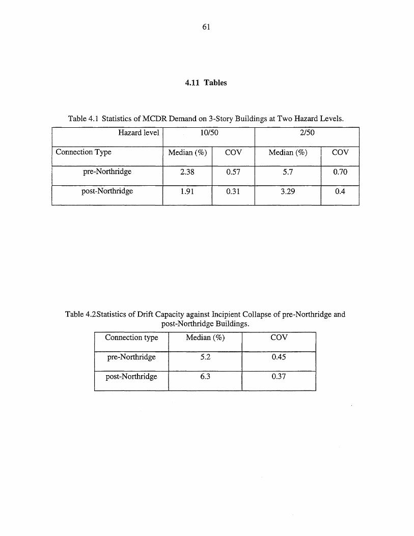
61
4.11 Tables
Table 4.1 Statistics of MCDR Demand on 3-Story Buildings at Two Hazard Levels.
Hazard level 10/50 2/50
Connection Type Median (%) COY Median (%) COY
pre-Northridge 2.38 0.57 5.7 0.70
post-Northridge 1.91 0.31 3.29 0.4
Table 4.2Statistics of Drift Capacity against Incipient Collapse of pre-Northridge and post-Northridge Buildings.
Connection type Median (%) COY
pre-Northridge 5.2 0.45
post-Northridge 6.3 0.37
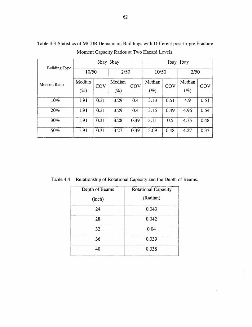
62
Table 4.3 Statistics of MCDR Demand on Buildings with Different post-to-pre Fracture
Moment Capacity Ratios at Two Hazard Levels.
3bay_3bay 1bay_1bay Building Type
10/50 2/50 10/50 2/50
Moment Ratio Median Median Median Median
COY COY COY COY (%) (%) (%) (%)
10% 1.91 0.31 3.29 0.4 3.13 0.51 4.9 0.51
20% 1.91 0.31 3.29 0.4 3.15 0.49 4.96 0.54
30% 1.91 0.31 3.28 0.39 3.11 0.5 4.75 0.48
50% 1.91 0.31 3.27 0.39 3.09 0.48 4.27 0.33
Table 4.4 Relationship of Rotational Capacity and the Depth of Beams.
Depth of Beams Rotational Capacity
(inch) (Radian)
24 0.043
28 0.042
32 0.04
36 0.039
40 0.038
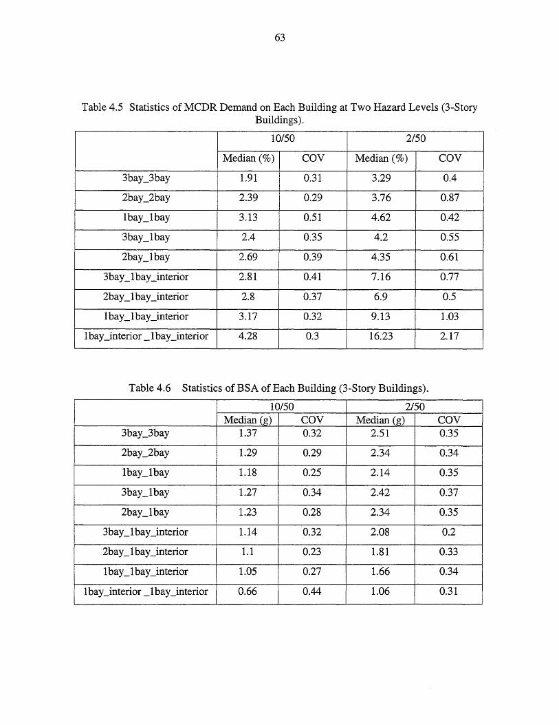
63
Table 4.5 Statistics of MCDR Demand on Each Building at Two Hazard Levels (3-Story Buildings).
10/50 2/50
Median (%) COY Median (%) COY
3bay_3bay 1.91 0.31 3.29 0.4
2bay_2bay 2.39 0.29 3.76 0.87
1bay_1bay 3.13 0.51 4.62 0.42
3bay_1bay 2.4 0.35 4.2 0.55
2bay_1bay 2.69 0.39 4.35 0.61
3bay _1 bay_interior 2.81 0.41 7.16 0.77
2bay _1 bay_interior 2.8 0.37 6.9 0.5
1 bay _1 bay_interior 3.17 0.32 9.13 1.03
1 bay_interior _1 bay_interior 4.28 0.3 16.23 2.17
Table 4.6 Statistics of BSA of Each Building (3-Story Buildings).
10/50 2/50 Median (g) COY Median (g) COY
3bay_3bay 1.37 0.32 2.51 0.35
2bay_2bay 1.29 0.29 2.34 0.34
1bay_1bay 1.18 0.25 2.14 0.35
3bay_1bay 1.27 0.34 2.42 0.37
2bay_1bay 1.23 0.28 2.34 0.35
3bay _1 bay_interior 1.14 0.32 2.08 0.2
2bay _1 bay_interior 1.1 0.23 1.81 0.33
1 bay _1 bay_interior 1.05 0.27 1.66 0.34
1 bay_interior _1 bay_interior 0.66 0.44 1.06 0.31

64
Table 4.7 Statistics of Capacities (MCDR) of Each Building (3-Story Buildings).
Median (%) of MCDR COY
3bay_3bay 6.3 0.37
2bay_2bay 6.9 0.19
1 bay_1 bay 4.86 0.64
3bay_1bay 5.97 0.31
2bay_1bay 6.08 0.18
3bay _1 bay_interior 6.37 0.23
2bay _1 bay_interior 7.43 0.15
1 bay _1 bay_interior 6.6 0.31
1 bay_interior _1 bay_interior 7.06 0.24
Table 4.8 Structural Demand (MCDR) for 3bay _3bay Building with Three
Different Modeling~
10/50 2/50
Median COY Median COY
(%) (%)
3-D modeling with elastic-plastic 1.91 0.31 3.29 0.4
column (ten elements in one story)
2-D modeling with elastic-plastic 1.57 0.21 3.16 0.14
column (ten elements in one story)
2-D modeling with lumped-plasticity 2.02 0.17 3.71 0.55
column (one element in one story)

65
Table 4.9 Statistics of Capacities of 3bay _3bay Building with Different Modeling (3-
Story)
Median (%) of COY
MCDR
3-D modeling with elastic-plastic column (ten 6.3 0.37
elements in one story)
2-D modeling with elastic-plastic column (ten 8.45 0.22
elements in one story)
2-D modeling with lumped-plasticity column (one 10.01 0.25
element in one story)
Table 4.10 Comparison of System Capacity (MCDR) for 2D Building with Different
Modelings-( 1).
Type of column
Ground Motion Elastic-plastic Lumped-plasticity
LA21 11.43 13.5 LA23 7.56 7.98 LA25 5.89 6.21 LA27 8.31 10.57 LA29 9.94 14.31 LA31 6.83 8.88 LA33 7.79 8.69 LA35 7.06 9.12
LA37 9.62 11.15
LA39 12.14 12.78
median 8.45 10.01
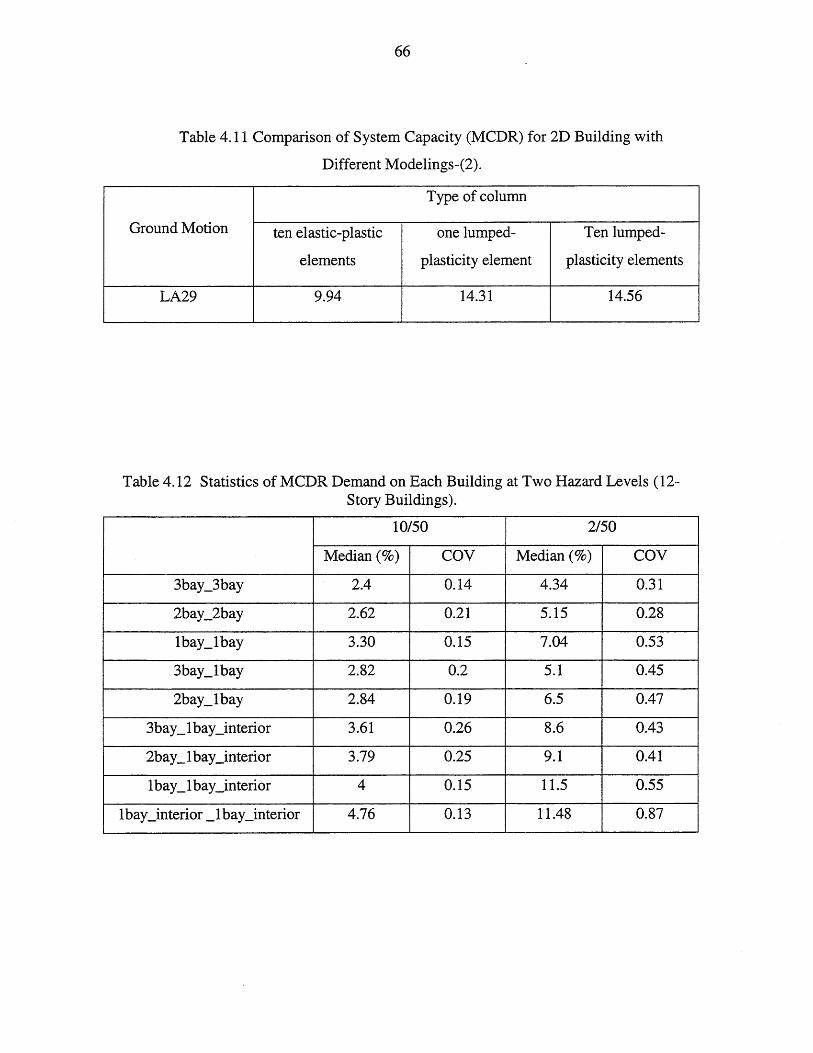
66
Table 4.11 Comparison of System Capacity (MCDR) for 2D Building with
Different Modelings-(2).
Type of column
Ground Motion ten elastic-plastic one lumped- Ten lumped-
elements plasticity element plasticity elements
LA29 9.94 14.31 14.56
Table 4.12 Statistics of MCDR Demand on Each Building at Two Hazard Levels (12-Story Buildings).
10/50 2/50
Median (%) COY Median (%) COY
3bay_3bay 2.4 0.14 4.34 0.31
2bay_2bay 2.62 0.21 5.15 0.28
1 bay_1 bay 3.30 0.15 7.04 0.53
3bay_lbay 2.82 0.2 5.1 0.45
2bay_lbay 2.84 0.19 6.5 0.47
3bay _1 bay_interior 3.61 0.26 8.6 0.43
2bay _1 bay_interior 3.79 0.25 9.1 0.41
1 bay _1 bay_interior 4 0.15 11.5 0.55
1 bay_interior _1 bay_interior 4.76 0.13 11.48 0.87
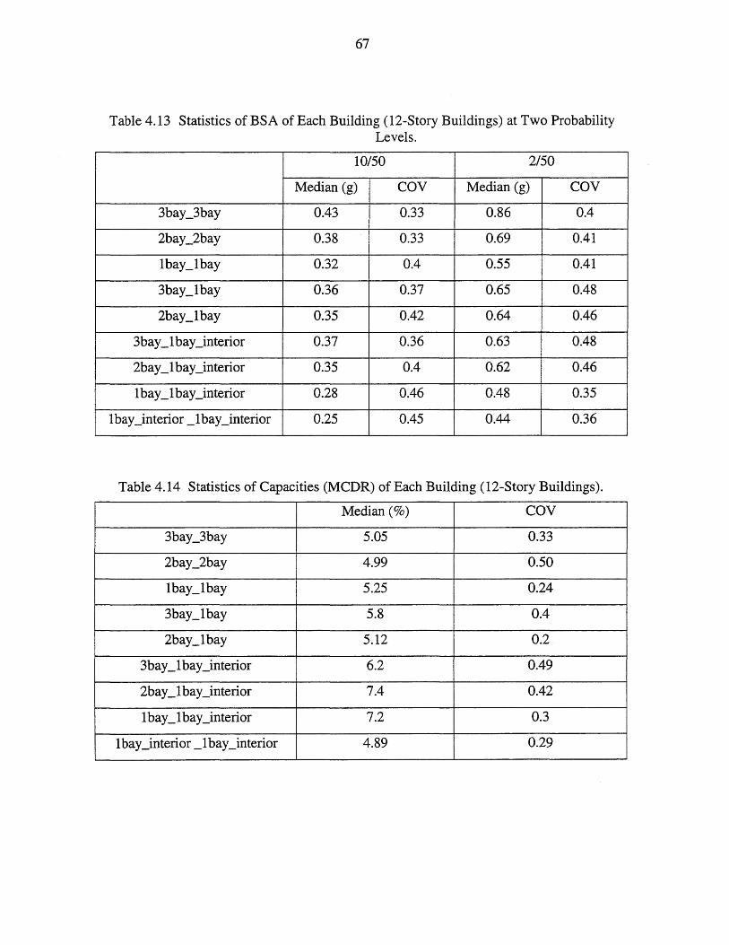
67
Table 4.13 Statistics of BSA of Each Building (12-Story Buildings) at Two Probability Levels.
10/50 2/50
Median (g) COY Median (g) COY
3bay_3bay OA3 0.33 0.86 0.4
2bay_2bay 0.38 0.33 0.69 OA1
1 bay_1 bay 0.32 OA 0.55 OA1
3bay_1bay 0.36 0.37 0.65 OA8
2bay_1bay 0.35 0.42 0.64 0.46
3bay _1 bay_interior 0.37 0.36 0.63 0.48
2bay _1 bay_interior 0.35 0.4 0.62 0.46
1 bay _1 bay_interior 0.28 0.46 0.48 0.35
1 bay_interior _1 bay_interior 0.25 0.45 0.44 0.36
Table 4.14 Statistics of Capacities (MCDR) of Each Building (12-Story Buildings).
Median (%) COY
3b ay_3 bay 5.05 0.33
2bay_2bay 4.99 0.50
1bay_1bay 5.25 0.24
3bay_1bay 5.8 0.4
2bay_1bay 5.12 0.2
3bay _1 bay_interior 6.2 0.49
2bay _1 bay_interior 7.4 OA2
1 bay _1 bay_interior 7.2 0.3
1 bay_interior _1 bay_interior 4.89 0.29
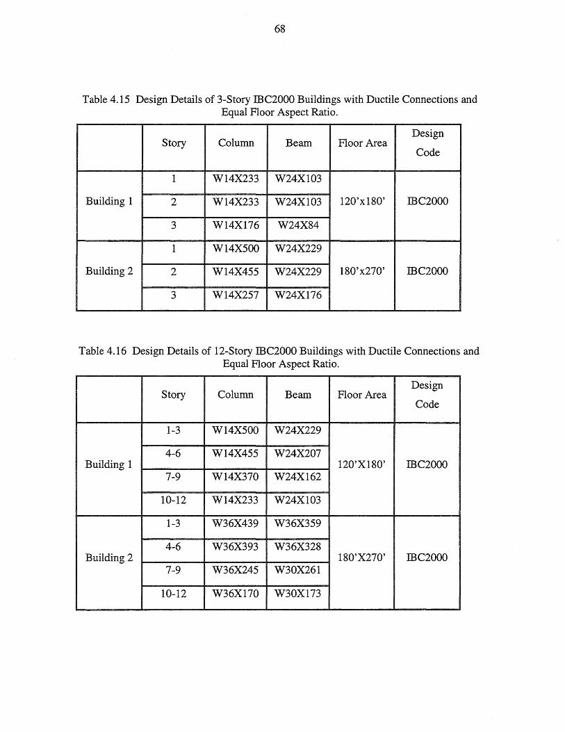
68
Table 4.15 Design Details of 3-Story IBC2000 Buildings with Ductile Connections and Equal Floor Aspect Ratio.
Story Column Beam Floor Area Design
Code
1 W14X233 W24X103
Building 1 2 W14X233 W24X103 120'x180' IBC2000
3 W14X176 W24X84
1 W14X500 W24X229
Building 2 2 W14X455 W24X229 180'x270' IBC2000
3 W14X257 W24X176
Table 4.16 Design Details of 12-Story IBC2000 Buildings with Ductile Connections and Equal Floor Aspect Ratio.
Story Column Beam Floor Area Design
Code
1-3 W14X500 W24X229
4-6 W14X455 W24X207 Building 1 120'X180' IBC2000
7-9 W14X370 W24X162
10-12 W14X233 W24X103
1-3 W36X439 W36X359
4-6 W36X393 W36X328 Building 2 180'X270' IBC2000
7-9 W36X245 W30X261
10-12 W36X170 W30X173

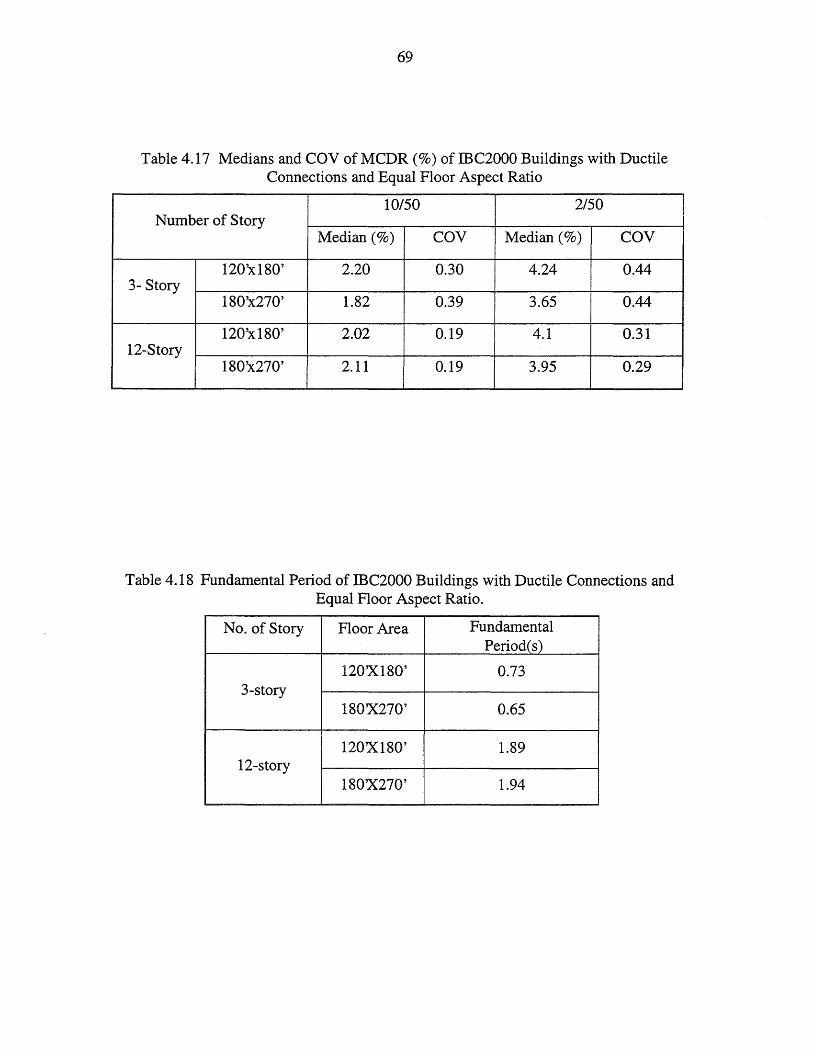
69
Table 4.17 Medians and COY of MCDR (%) of IBC2000 Buildings with Ductile Connections and Equal Floor Aspect Ratio
10/50 2/50 Number of Story
Median (%) COY Median (%) COY
120'x180' 2.20 0.30 4.24 0.44 3- Story
180'x270' 1.82 0.39 3.65 0.44
120'x180' 2.02 0.19 4.1 0.31 12-Story
180'x270' 2.11 0.19 3.95 0.29
Table 4.18 Fundamental Period of IBC2000 Buildings with Ductile Connections and Equal Floor Aspect Ratio.
No. of Story Floor Area Fundamental Period(s)
120X180' 0.73 3-story
180X270' 0.65
120X180' 1.89 12-story
180X270' 1.94
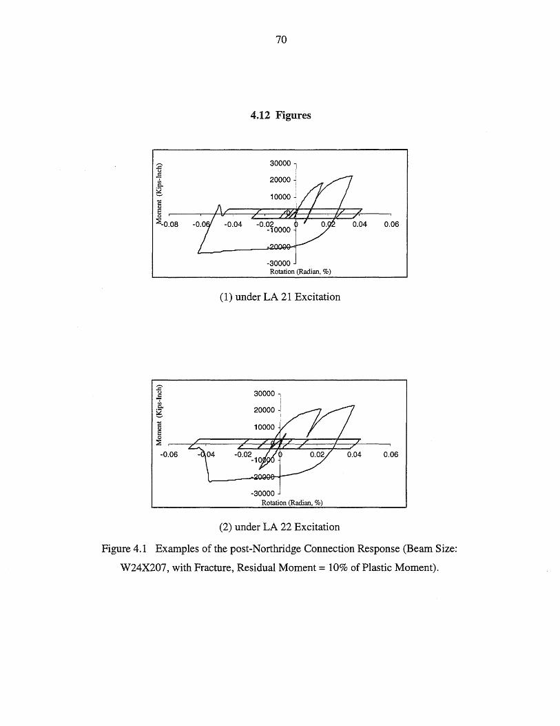
70
4.12 Figures
:a- 30000 u
1 20000 c. g
10000
~ o ~-0.08 -0.04 -O.~foooo 0.06
-30000 Rotation (Radian, %)
(1) under LA 21 Excitation
:a-~
30000
c.. g
~ o ~
-0.06 0.06
-30000 Rotation (Radian, %)
(2) under LA 22 Excitation
Figure 4.1 Examples of the post-Northridge Connection Response (Beam Size:
W24X207, with Fracture, Residual Moment = 10% of Plastic Moment).
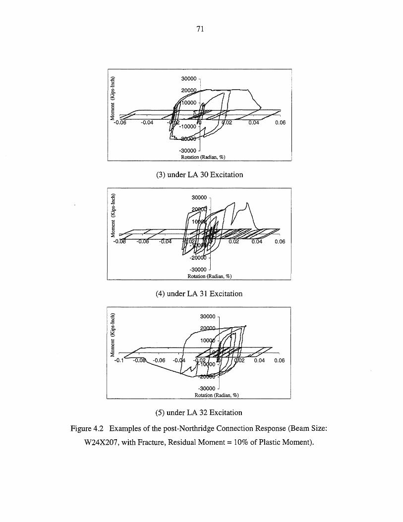
2 t)
~
~ i o ~ -0.
2 t) c '"i'
~ i ~
-0.1
71
-30000 Rotation (Radian, %)
(3) under LA 30 Excitation
30000
-30000 Rotation (Radian, %)
(4) under LA 31 Excitation
30000
0.06
-30000 Rotation (Radian, %)
(5) under LA 32 Excitation
Figure 4.2 Examples of the post-Northridge Connection Response (Beam Size:
W24X207, with Fracture, Residual Moment = 10% of Plastic Moment).

c E ~
-0.08
72
30000
0.06 0.08
-30000 Rotation (Radian, %)
(1) under LA 21
30000
0.06 0.08
-30000 Rotation (Radian, %)
(2) under LA 22
Figure 4.3 Examples of the post-Northridge Connection Response (Beam Size:
W24X279, without Fracture).
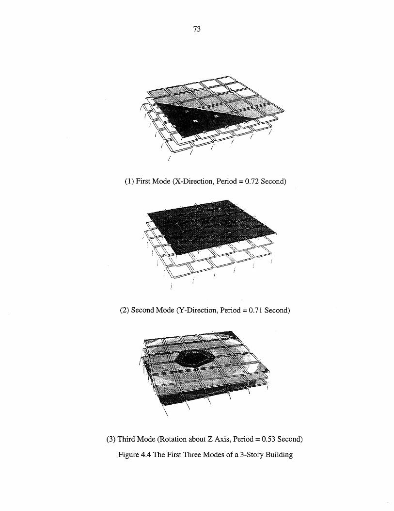
73
i
(1) First Mode (X-Direction, Period = 0.72 Second)
(2) Second Mode (Y-Direction, Period = 0.71 Second)
(3) Third Mode (Rotation about Z Axis, Period = 0.53 Second)
Figure 4.4 The First Three Modes of a 3-Story Building
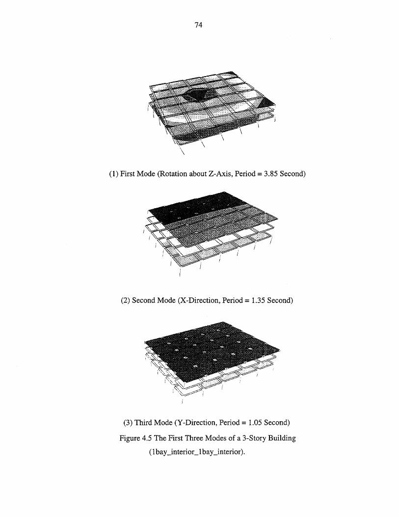
74
(1) First Mode (Rotation about Z-Axis, Period = 3.85 Second)
(2) Second Mode (X-Direction, Period = 1.35 Second)
(3) Third Mode (Y -Direction, Period = 1.05 Second)
Figure 4.5 The First Three Modes of a 3-Story Building
(1 bay _interior_l bay_interior).
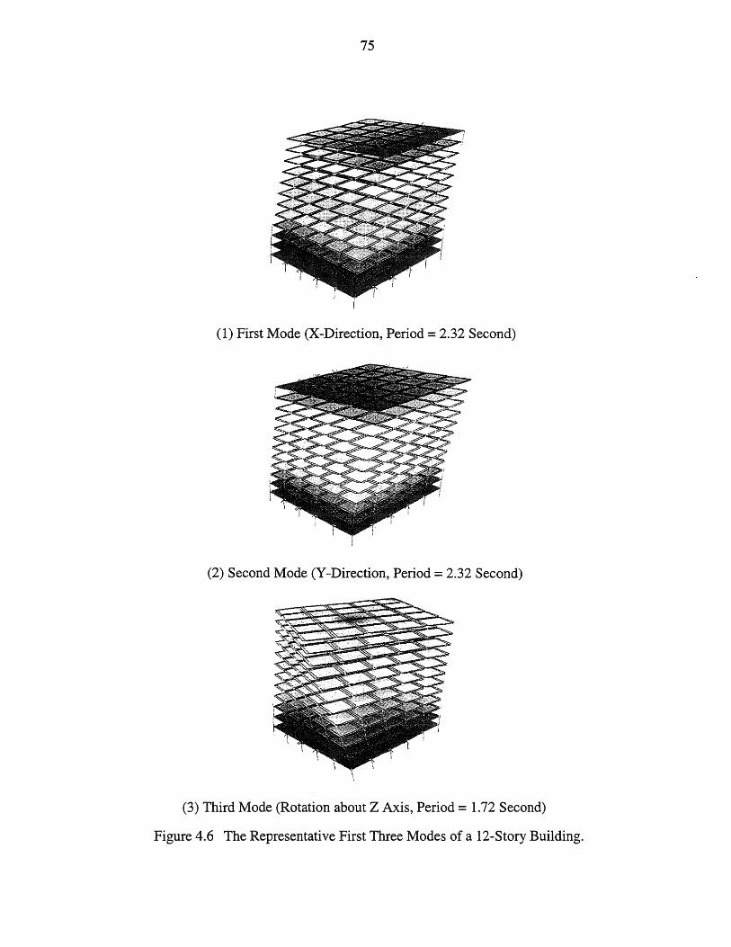
75
(1) First Mode (X-Direction, Period = 2.32 Second)
(2) Second Mode (Y -Direction, Period = 2.32 Second)
(3) Third Mode (Rotation about Z Axis, Period = 1.72 Second)
Figure 4.6 The Representative First Three Modes of a 12-Story Building.
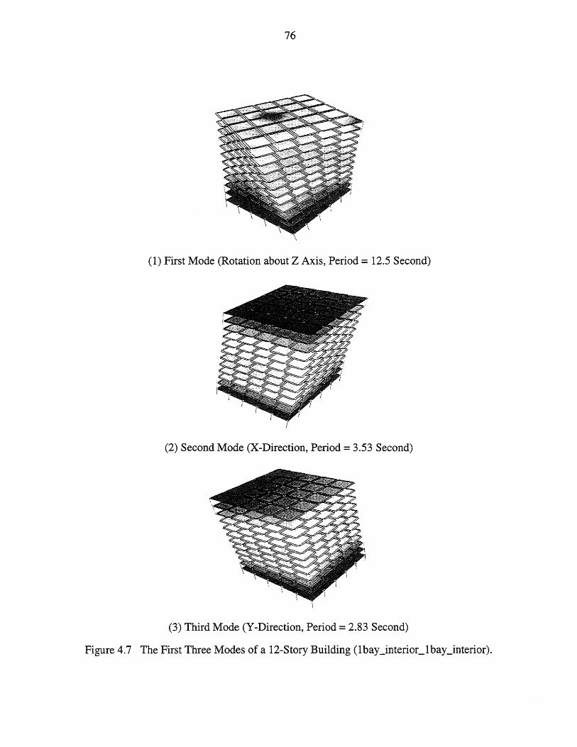
76
(1) First Mode (Rotation about Z Axis, Period = 12.5 Second)
(2) Second Mode (X-Direction, Period = 3.53 Second)
(3) Third Mode (Y -Direction, Period = 2.83 Second)
Figure 4.7 The First Three Modes of a 12-Story Building (lbay_interior_1bay_interior).
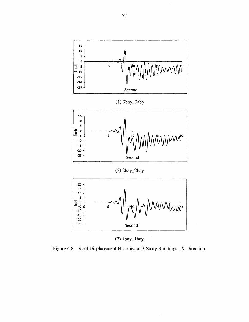
15
10
5
77
o+-------__ ~~~~~--~--~--------~ '"§ -5
== ~-10
-15
-20
-25
15
10 5
5
Second
'"§ o+-------~~~++~~--------~--------~ tS -5
-10 -15
-20
-25
20 15 10
..r:: 5
5
Second
(2) 2bay _2bay
g 0 +----~~PrI_+++-~-H---_I+__I\__j~,....._w__:__--~
- -5 5 -10 -15 -20 -25 Second
Figure 4.8 Roof Displacement Histories of 3-Story Buildings, X-Direction.
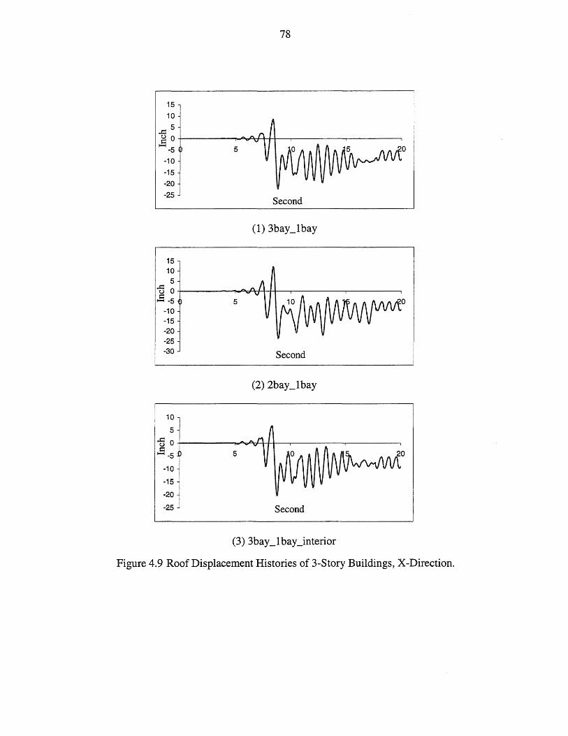
78
15
10
,.s::::5 C) 0 +------T"~Od_++~_,__---___,----__, ~
-5
-10
-15
-20
-25
15 10 5
5
Second
~ O+---------T"~R+++~_,__---___,----__, ~ -5
-10 -15
-20 -25 -30
10
5
Second
5
~O+-------,..,Ag.~++-~--,-----___,,--------,
= ~ -5
-10
-15
-20
-25
5
Second
(3) 3bay _1 bay_interior
Figure 4.9 Roof Displacement Histories of 3-Story Buildings, X-Direction.
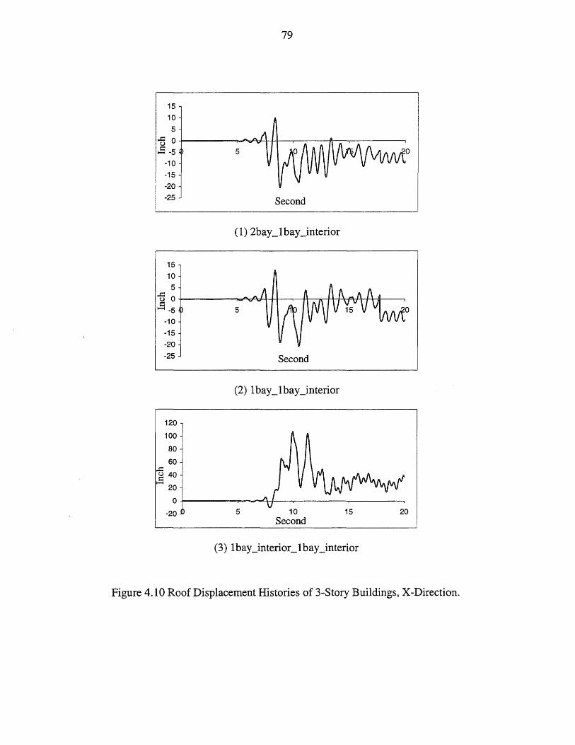
15
10
5
79
~ 0+-------~~~++~~----4r~~------~
~ -5
-10
-15
-20
-25
15
10
5
5
Second
~0+-----_..A::PJ-+-I--l----'----H-----"--H-..f-.\-,~H-4r-A-----' 1=:1
...... -5
..c:::
-10
-15
-20
-25
120
100
80
60
u 40
~ 20
5
Second
O+--------~--~~--~------~------~
-20 5 10 Second
15 20
Figure 4.10 Roof Displacement Histories of 3-Story Buildings, X-Direction.
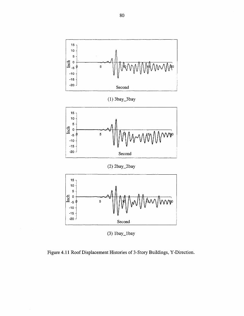
15
10
5
80
~ O+-------____ ~rH~~----~~~----~~
= ~ -5
-10
-15
-20
15
10
5
5
Second
~ O+-----------~~~~------~--------~ ~
-5
-10
-15
-20
15
10
5
5
Second
~ O+-------__ ~~++~~~--~~~--~--~ = ~ -5 5
-10
-15
-20 Second
Figure 4.11 Roof Displacement Histories of 3-Story Buildings, Y -Direction.
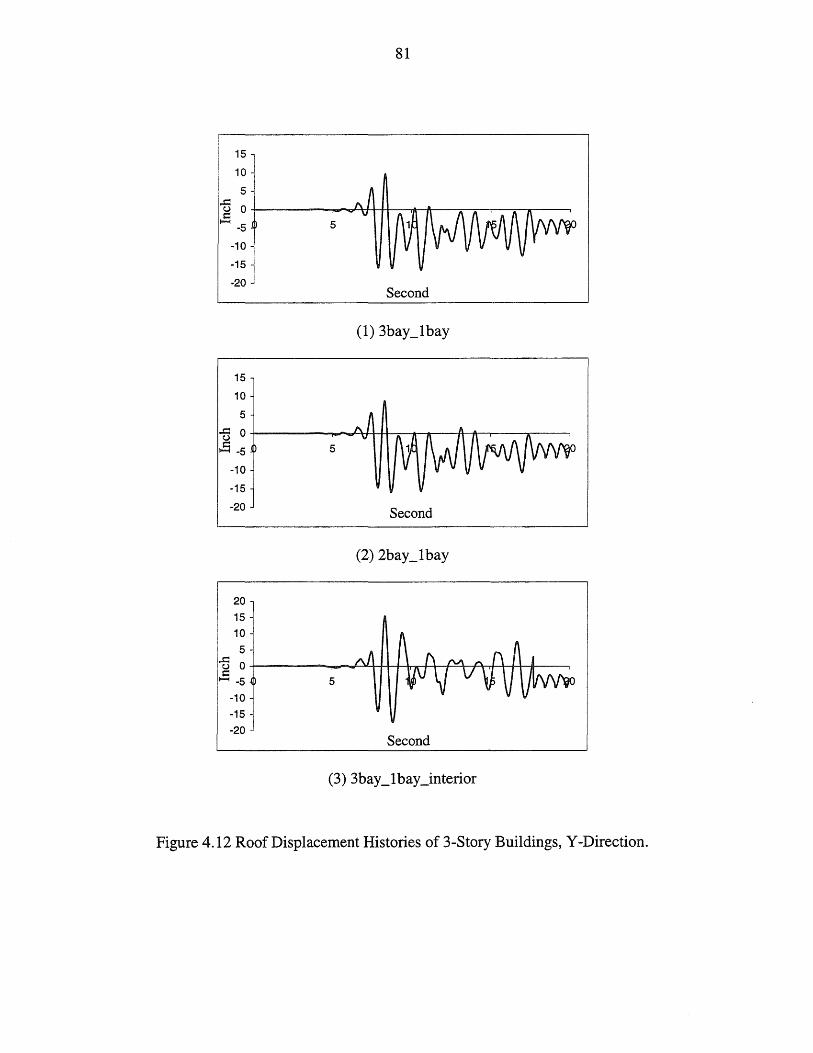
15
10
5
81
..= u 0+-------~_v+H~--~~~~~~~--~
toS -5
-10
-15
-20
15
10
5
5
Second
~ O+-------~_J~rl+~~ __ ~~~--~--~
toS -5
-10
-15
-20
20
15
10
5
5
Second
~ O+-------__ --~H4~hrlHr~~~~~~~ \:: ~ -5 5
-10
-15
-20 Second
(3) 3bay_lbay_interior
Figure 4.12 Roof Displacement Histories of 3-Story Buildings, Y -Direction.
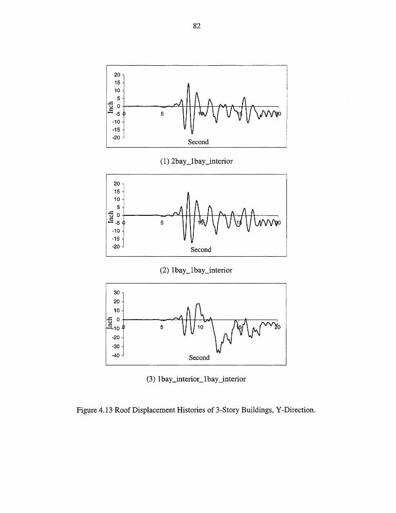
20
15
10
5
82
~ o+-------____ ~++~~++_A~~++~----~ ~ ~ -5
-10
-15
-20
20
15
10
5
5
Second
~ O+-------__ ~~~~+_~~~~++~----~ ~ ~ -5
-10
-15
-20
30 1 20
10
5
Second
~ O+-------____ ~++~~~----~_+------~ g ~-10 5
-20
-30
-40 Second
Figure 4.13 Roof Displacement Histories of 3-Story Buildings, Y -Direction.
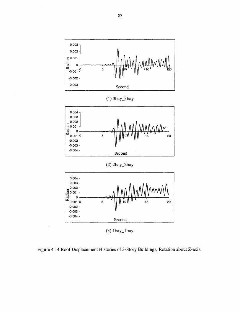
0.003
0.002
=0.001 ~
83
~ 0+-------~~~rt4#+~~~~~~~~+H ~
-0.001
-0.002
-0.003
0.004
0.003
0.002
.§ 0.001
5
Second
~ 0+---------~~M4~~~H+~4H~~~~ ~-O.001
-0.002
-0.003
-0.004
0.004
0.003
0.002
.§ 0.001
5 20
Second
~ O+-------~~~HH~~~~~~------~ ~-0.001 5
-0.002
-0.003
-0.004 Second
Figure 4.14 Roof Displacement Histories of 3-Story Buildings, Rotation about Z-axis.

0.003
0.002
§ 0.001
84
~ o+-------~~~~~----~~~------~ Cd ~0.001
-0.002
-0.003
-0.004
-0.005
0.004
0.002 §
5
Second
~ O+-------~~~~+H~~~~~~~~~ ~
-0.002
-0.004
-0.006
0.002
§ 0.001
5 20
Second
(2) 2bay _1 bay
~ O+---------AJ~~~----~~~------~ ~0.001
-0.002
-0.003
-0.004
-0.005
-0.006
5 20
Second
Figure 4.15 Roof Displacement Histories of 3-Story Buildings, Rotation about Z-axis.
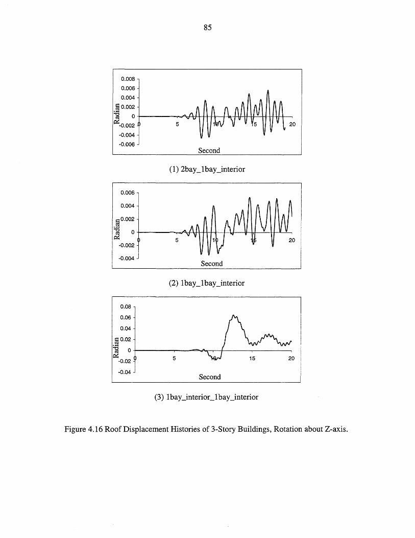
85
0.008
0.006
0.004
fa 0.002 :.a 0 cd
~-0.002 5 20
-0.004
-0.006 Second
0.006
0.004
a 0.002
~ o+---------~~~HH~~~~M-~~~~ ~ 5
-0.002
-0.004 Second
0.08
0.06 !\ 0.04
a 0.02 _ _ I vvvAl~"W'I ~ O+-------~----~~~~~'~ I----~~------~ ~-0.02 ~ 5 .~ 15 20
-0.04 Second
Figure 4.16 Roof Displacement Histories of 3-Story Buildings, Rotation about Z-axis.
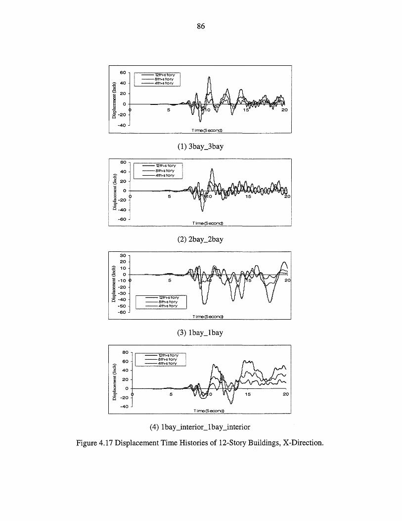
86
60 -- l2th-s tory --8th-story --4th-story
-40 T Ime(S ecx::>n:::!>
60 --12th-s tory
40 --8th-s tory
-5 --4th-s tory
e 20
~ O+----------.~~~~~~~~Md~~~~HH~~ ] -20 s;-0-40
-60
30
20
:2 10
5
T lme (S ecx::>n:::!>
~ O+---------~~~~~~~~~~~~~~,,~~
I ~~~ -a -30
a -40
-50
-60
80
60 :2 u 40 e c 20 ~ 8 0 e<:I c.. a -20
-40
5
--l2th-s tory --8th-story --4th-s tory
T lme (S econc:!>
(3) Ibay_lbay
-- l2th-s tory --8th-s tory --4th-story
5
T ime (S ecx::>n:::!>
(4) Ibay_interior_lbay_interior
Figure 4.17 Displacement Time Histories of 12-Story Buildings, X-Direction.

40
30
:c 20
:§. 10
87
-- l2th-s tory --8th-s tory --4th-story
~ o+---~----~~~~~~~~~~~~~~~ ~ -10 5
~-20 Q
-30
-40
40
30
:c 20
:§. 10
T Irre (S a:::onoj
-- 12th-s tory --8th-s tory --4th-s tory
~ o+---------~~~~~~~~~~~~~~~~~~ 8 -10 5 0:1 ~-20
Q -30
-40
-50
60
-5 40
e 20
T Irre (S e::oncj)
-- l2th-s tory --8th-s tory --4th-story
~ O+---------~~~~~~~~~~_m~~~~~~~ ~ -a. -20
is -40
-60
30
20 10
5
T Irre (S e::oncj)
(3) Ibay_lbay
-5 e O+---------~~~~~~~~~~--~~~~~~= c -10 5
~ -20
~ -30
~-40 Q -50
-60
--12th-s tory --8th-story --4th-s tory
T Irre(Se::oncj)
(4) Ibay_interior_lbay_interior
Figure 4.18 Displacement Time Histories of 12-Story Buildings, Y-Direction.
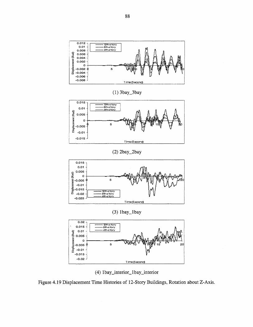
0.012 0.01
0.008 ~ 0.006 g 0.004
~ 0.002
88
--12th-s tory --8th-s tory --4th-story
§ o+---------~ __ ~~~~~~~4_~~~~~~ -a -0.002 is -0.004
-0.006 -0.008
0.015
0.01 ~ g 0.005
5
T Irre (S e:::x:>ncP
--l2th-s tory --8th-story --4th-sto
~ 0 +------"""""" ......... ~MM~\l__A~~~Dhr::_:o.\ 8 i -0.005
is -0.01
-0.015
0.015
0.01
~ 0.005
5
T Irre (S e:::x:>ncP
g O+---------~--__ ~~~~~~~~~~~~~~ ~ -0.005
8 -0.01 0:1
~-0.015
is -0.02
-0.025
0.02
T Irre (S e:::x:>ncP
--12th-s tory --8th-story --4th-story
0.015
~ 0.01
g 0.005 i:: ~ O+-------~--~~~~~~~~~~~~~
~-0.005 -a is -0.01
-0.015
-0.02
5
T Irre (S e:::x:>ncP
(4) 1bay_interior_1bay_interior
Figure 4.19 Displacement Time Histories of 12-Story Buildings, Rotation about Z-Axis.
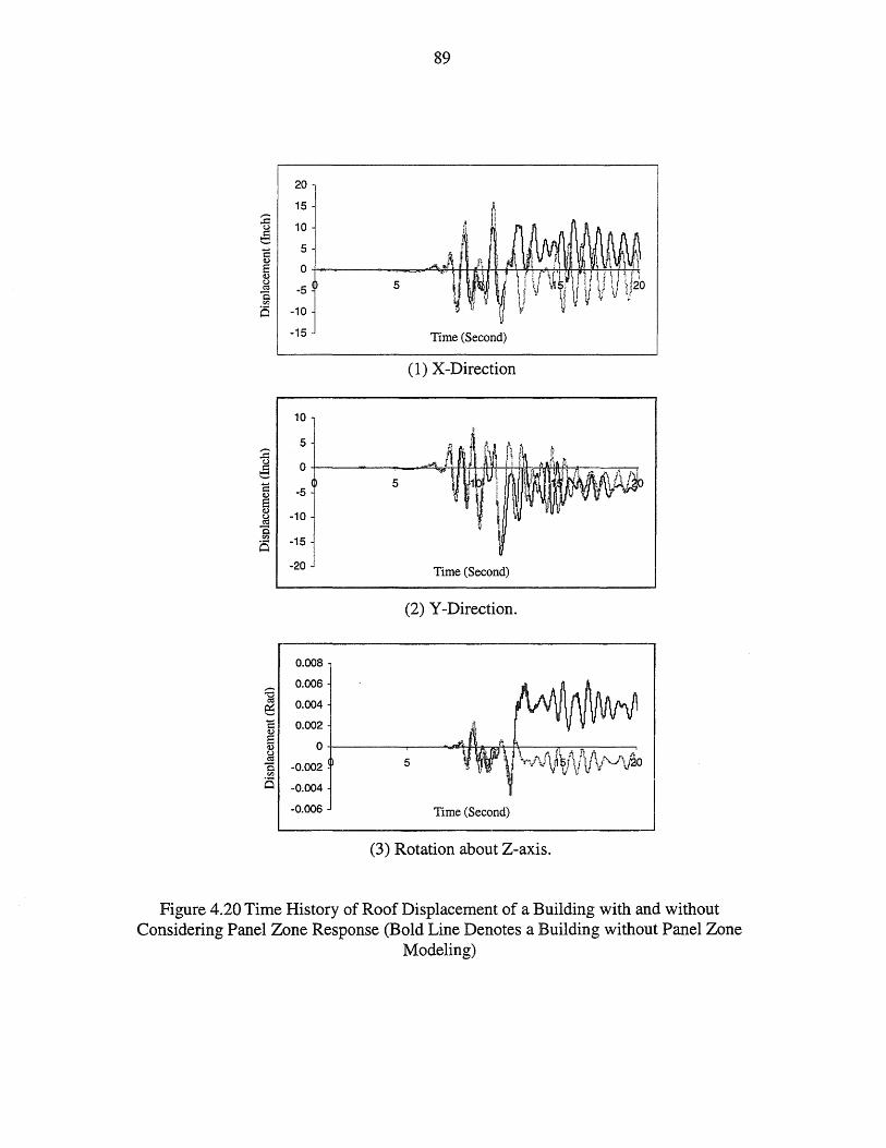
89
20
15 ;c u 10 e
5
Or-------~~~~HHHr~~r~~~~4f~
-5 5
-10
-15 Time (Second)
(1) X-Direction
10
5 ;c ~ O+-----------~ __ ~~~HH~~~~~~----~~
5 -5
-10
-15
-20 Time (Second)
(2) Y-Direction.
0.008
~ 0.006
CI:l 0.004 ~ "5 0.002 E 0 Q) u CI:l
-0 -0.002 5
"" 0 -0.004
-0.006 Time (Second)
(3) Rotation about Z-axis.
Figure 4.20 Time History of Roof Displacement of a Building with and without Considering Panel Zone Response (Bold Line Denotes a Building without Panel Zone
Modeling)
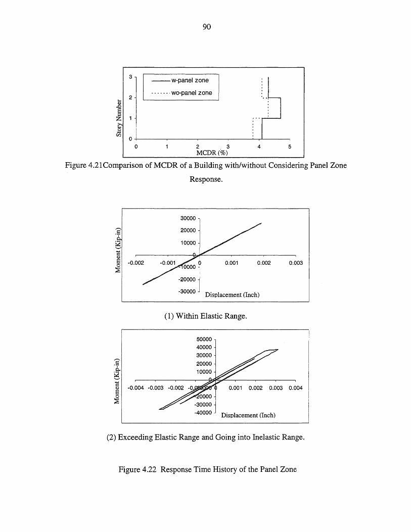
90
3 --w-panel zone
2 - - _. - _. wo-panel zone
'--,-I-< Q)
..0 S ::l
1 Z .• --~ ~ .8 lZ)
0
0 2 3 4 5 MCDR(%)
Figure 4.21 Comparison of MCDR of a Building with/without Considering Panel Zone
Response.
30000
-30000 Displacement (Inch)
(1) Within Elastic Range.
50000
40000 30000 20000
-40000 Displacement (Inch)
0.003
(2) Exceeding Elastic Range and Going into Inelastic Range.
Figure 4.22 Response Time History of the Panel Zone
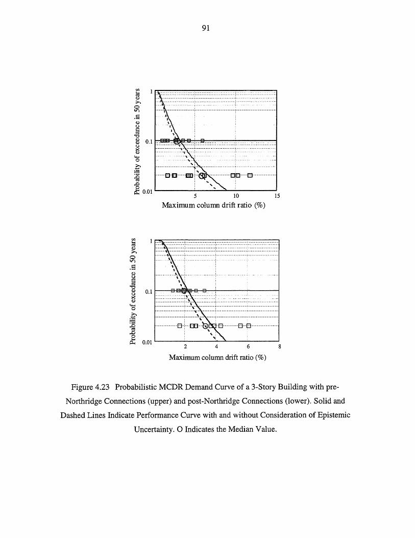
tI.l
~ >. o VI
.S (1) u ~
"'0
91
§ 0.1 ~.~ ........ ~ ....... ~ ......... ~ ... ~2t:===E===j ~ .: ......... ~ .. ~\:: ............ : ............................................................... , ................................. ·····························1
>. ... :.=
·····El········ ii .g ~ 0.01 1.-..-----i.5--..;;.....~--'-1O-----J15
(1) u a
13
Maximum column drift ratio (%)
~ .. !., .. , ........................ .
(1) ........................:, .. "-............................. ; ................................................ : ............................. ··· .. ··· ......... 1
0.1 t---8-!i:!HfiJ!iHH:3--l:3---'------------i
~ .......................... ~~~~ .... ~~~~.:~~~ ... ~.~; ..... ~:.::.~:~;~": ...... ,, ........ : ......... : ................ ,': .•...... : ......... : •....... : .......... : ....... : ....... : ........ : .. "; .. :: ...... : ..... : ....... : ... : .. : .... : ........ 11
~ ................................•...... , ..•.............. ~., ... " ......................................................... ·····················································1
~ ............. e ......... EEl ... @ .. . .J::J . '.~ : 8 ~ ~ 0.01 L...-__ --'-___ --'--.l.... __ -'---__ --I
246 8
Maximum column drift ratio (%)
Figure 4.23 Probabilistic MCDR Demand Curve of a 3-Story Building with pre
Northridge Connections (upper) and post-Northridge Connections (lower). Solid and
Dashed Lines Indicate Performance Curve with and without Consideration of Epistemic
Uncertainty. 0 Indicates the Median Value.
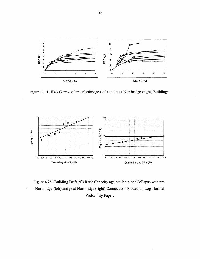
92
10 15 20 25
MCDR(%)
10
8
6
o~,~--~----~--~----~--~
o 5 10 15
MCDR(%)
Figure 4.24 IDA Curves of pre-Northridge (left) and post-Northridge (right) Buildings.
2' o u 6 !:' .~ Q. CI1 U
1~--~~~----~--~----~~ 6.7 10.6 15.9 227 30.940.1 50 59.9 69.1 773 84.1 89.4 93.3
Cumulative prooability (%)
2 o U
1"'1·········,················
. ,
;... ..... ....... ..... ;
.; . .:
;1OF=~ .. ,.~==~~~~~=-~~~ .. ~""~?""~f:;.~ ... ""="~D-~ 'g I ~--r ...... ,.. , ... . ~ p=, U '
.
.
6.7 10.6 15.9 22.7 30.9 40.1 SO 59.9 69.1 77.3 84.1 89.4 93.3
Cumulative probability (%)
Figure 4.25 Building Drift (%) Ratio Capacity against Incipient Collapse with pre
Northridge (left) and post-Northridge (right) Connections Plotted on Log-Normal
Probability Paper.
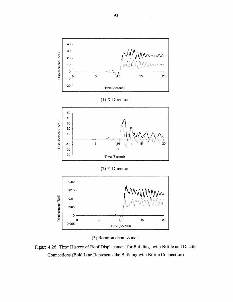
93
5 15 20
Time (Second)
(1) X-Direction.
50
40
:2 30 u r:: 20 0
C 10 Q.)
e Q)
0 u CIS
'0 -10 j[) til 5 is
-20
-30 Time (Second)
(2) Y -Direction.
0.02
0.015
::0 CIS 0.01 E:j C
0.005 Q.)
e Q.) u CIS '0 0
a 5 ~,p 15 20 -0.005
Time (Second)
(3) Rotation about Z-axis.
Figure 4.26 Time History of Roof Displacement for Buildings with Brittle and Ductile
Connections (Bold Line Represents the Building with Brittle Connection)
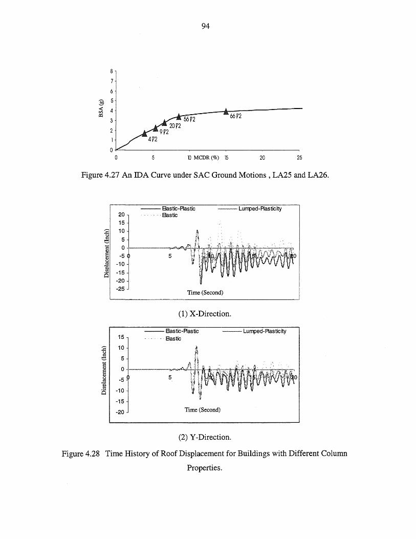
94
8
7
6
§ 5 <: 4 tf)
a:l 66V2 3
2
5 10 MCDR(%) 15 20 25
Figure 4.27 An IDA Curve under SAC Ground Motions, LA25 and LA26.
::2 u I: e c: Q)
e Q) u ro '0
CIl
Q
::2 u I: e c: Q)
e Q) u ro '0
CIl
Q
20
15
10
5
-~ I -10
-15
-20
-25
15
10
5
0
-5
-10
-15
-20
--Bastic-Plastic .......... Bastic
--Lumped-Plasticity
Time (Second)
(1) X-Direction.
--Bastic-Plastic ... Bastic
Time (Second)
--Lumped-Plasticity
(2) Y -Direction.
Figure 4.28 Time History of Roof Displacement for Buildings with Different Column
Properties.
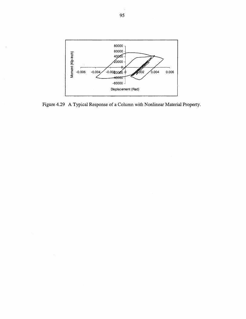
:c-o
.!;;
.9-~ E Q)
E -0.006 o :E
95
80000
-60000
Displacement (Rad)
0.006
Figure 4.29 A Typical Response of a Column with Nonlinear Material Property.
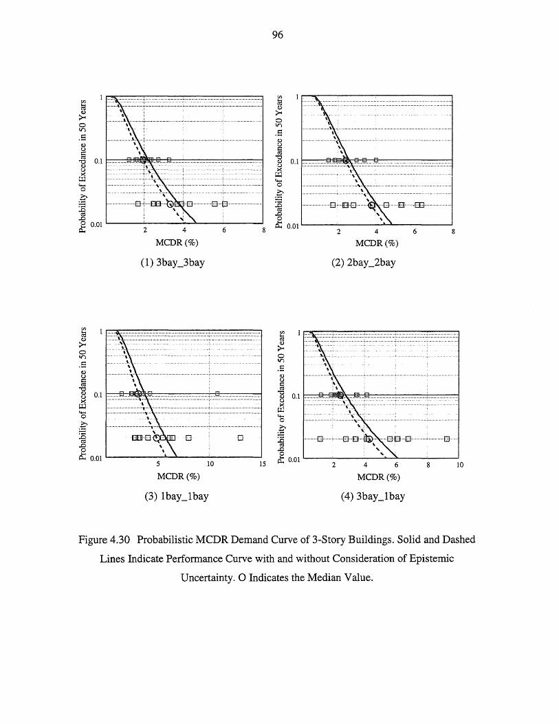
en ~ <L> ~ 0 V')
.5 <L> Co) t:: ro
"'CI <L> Co)
>< Ul <+-< 0
~ :.E ro
..0
1 ....
0.1 .. !.\ ... , ,." ............................... , ............................................ , ........................................... ,
............... , ..... , ,"'," ................... , ............. ,.. ..... " .................. , ........................................... ; ............................................ j ,
. " ........ ··············B·-+······EEl····~ , ... , .. , .... , .................... ++.++ ................. , ........ , .......... ~ ,
" ' , £ 0.01 2 4 6 8
en ~ <L> ~ o V')
.5 <L> Co) t:: ro
MCDR(%)
1 ......... .
"g ~ 0.1 ::::::.:.::.~::::.:::'.::.:.::.:.:: ..... ,'::~.
Ul ..................................... :.~ ..... \: ................................................................ ? ......................................................... ~ ....... o
~ :.E ro
.. ........................................ , ..... '\: .......................................................... · .. f ...... · ............ · ...................... · .............. ·~ , , ................................................. " ...................................................... , ............................................................ j
" [][DO o o ..0 o
I-< ~ 0.01 '--____ ~...:Io.-__________ ----J
5
MCDR(%)
10 15
96
en ~ CI,)
~ 0 V')
.5 <L> Co) t:: ro
"'CI CI,) Co)
>< Ul <+-< 0
~ :.E ro
..0 0 I-< ~
en ~ CI,)
~ o V')
.5 CI,) Co) s::: ro
"'CI CI,) Co)
>< Ul <+-< o
~ ~ ..0 o
0.1
0.01
.. ·[] .... ·IE .........
2 4
MCDR(%)
(2) 2bay_2bay
6 8
~ 0.01 '----'---------"--'6"""------------' 2 4 8 10
MCDR(%)
(4) 3bay_lbay
Figure 4.30 Probabilistic MCDR Demand Curve of 3-Story Buildings. Solid and Dashed
Lines Indicate Performance Curve with and without Consideration of Epistemic
Uncertainty. 0 Indicates the Median Value.
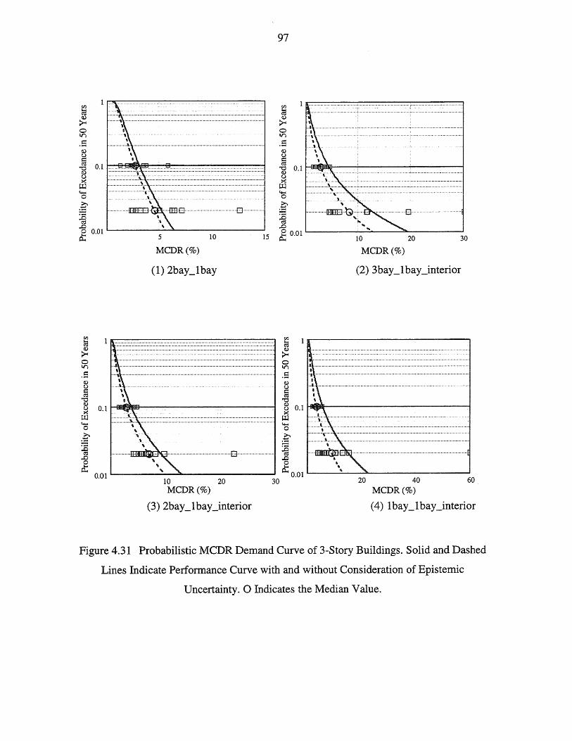
CI}
~ Q)
~ 0 tr)
.5 Q) u s:: t':3 0.1 '"0 Q) u >< ~
CI}
~ ~ 0 tr)
.5 Q) u s:: t':3
'"0 Q)
0.1 u >< ~ '+-< 0
g :.E
t':3 ..c
£ 0.01
5
MCDR(%)
10
(1) 2bay_1bay
············· .. ······B .. · .... · .... · ...... ·
.......................................... 8 .......... ·
10 20 MCDR(%)
(3) 2bay_1bay_interior
97
~ Q)
~ o tr)
.5 Q) u §
'"0 0.1 1-m1lBJm-----!-----....;----~ 8 .......... c·,·· ....................... ; ....................................................... ; ........................... · ...... ·· .. · .. ·· .. · .. · .. ··1
>< .......... \ ... ~ ..................... \ t) ..................... \.~
g .................. ~.~ .... i :g , '" ..... ..c ..
15 £ 0.01 10 20 30
MCDR(%)
(2) 3bay_1bay_interior
CI}
~ Q)
~ 0 tr)
.5 Q) u s:: t':3
'"0 Q)
0.1 u >< ~ '::"\::':'''.'' ........................................................................................................ .. t) ............ ~, ...... " .......................................................................................................................................... · .. 1 >. .............. " ................... . ~ .................. '-...... . , ~ ...... mmt1D .... ..c ...
30
8 \ ~ 0.01 L.-__ ,~_...:::a.-________ ......I
40 60 20 MCDR(%)
(4) 1bay_1bay_interior
Figure 4.31 Probabilistic MCDR Demand Curve of 3-Story Buildings. Solid and Dashed
Lines Indicate Performance Curve with and without Consideration of Epistemic
Uncertainty. 0 Indicates the Median Value.

o V"l
.5
98
.~\ ~ "t~\""""'''''''''''''''''''''''''''''''''''''''''''''''''''''''''''''''''''''''''''' .............................................................. , ..................... · .. ····· .... · .... 1
~ II ~ 0.1 ~:::::::!"~ ..... :~::::: .. ~==:==:==:?:E==:==:==:==:==:?:t==:==:1 ~ • ~~ ................................................... , ................................... ··· ...... ·········· .... ·· .. ·· .. ·· ...... ··• .. · ........ ··· ...... ···· .......... 1
.............. i ............... :.~"' ................................................. ; ........................................................................................................................ 1 , ~~ ............................................ i ........................................... .............................. , ....................................... 1
::::::::::::::~~<:::::::.~., ............................................................................................................................... · .... · .. · .................. 1
"EIIJ1'~~ [J
'.. " .......... '. ~ 0.01 L..-__ ~, __ '--~ _____ '--._----I
20 40 60 80 100
MCDR(%)
Figure 4.32 Probabilistic MCDR Demand Curve of 3-Story Buildings. Solid and Dashed
Lines Indicate Performance Curve with and without Consideration of Epistemic
Uncertainty. 0 Indicates the Median Value.
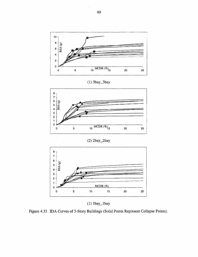
99
10
8
6
4
2
o 5 10 MCDR(%~5 20 25
8
7 6 :§ 5 <
IZl 4 a:l
3 2
1
0 10 MCDR (%)15 0 5 20 25
(2) 2bay _2bay
8
7
6 :§
5
4
3
2 --_ .. -_._ .. _ ... -1
MCDR %
5 10 15 20 25
(1) 1bay_1bay
Figure 4.33 IDA Curves of 3-Story Buildings (Solid Points Represent Collapse Points).

100
8
7
6 """' ~ 5 <::
CIl
4 a:l
3
2 -_ .. _._-_ ........ __ ....... 1
0 MCDR(%)
0 5 10 15 20 25
(1) 3bay_1bay
8
7
6 §
5
4
3
2
MCDR %
5 10 15 20 25
(2) 2bay_1bay
5
4 § <:: CIl
3 a:l ..-=-------2
MCDR(%) O~------~----~------~------~------~
o 5 10 15 20 25
(3) 3bay _1 bay_interior
Figure 4.34 IDA Curves of 3-Story Buildings (Solid Points Represent Collapse Points).
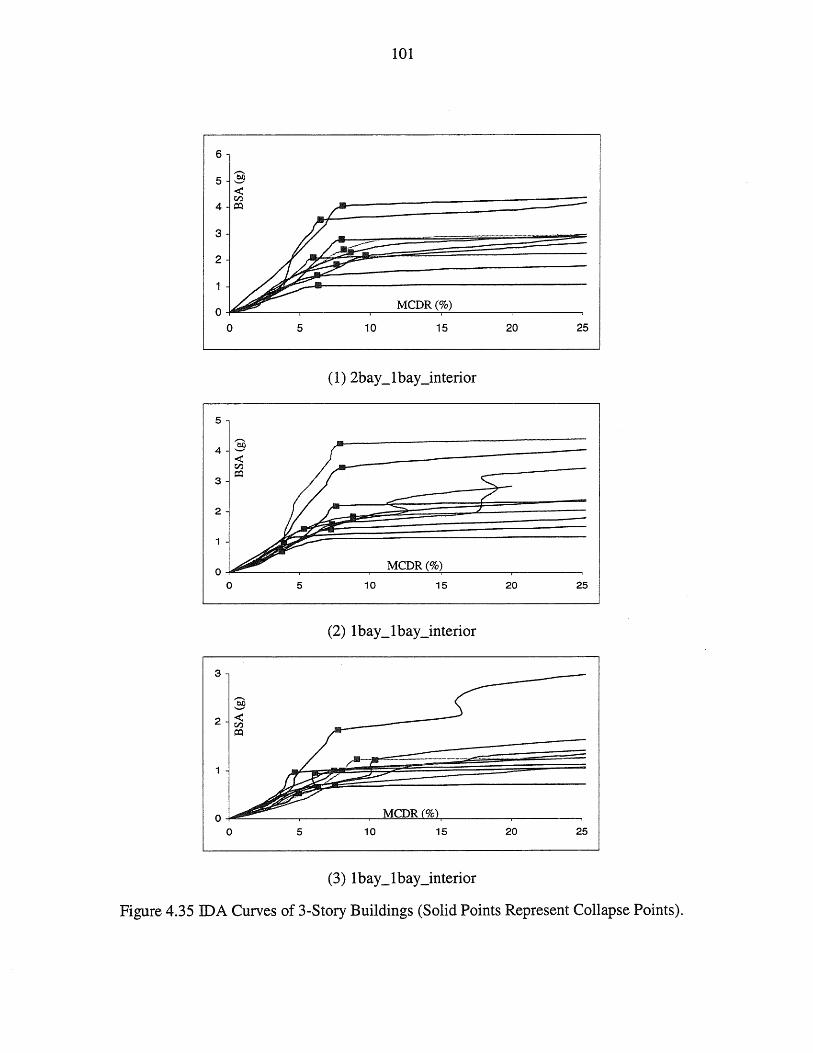
101
6
3
2
O~~ ____ ~ ____ ~ ___ M_C_D_R_(~%~) ______ ~ ____ ~
o 5 10 15 20 25
5
2
O~ ______ ~ ____ ~~M~CD~R~(~~o) ______ ~ ______ ~ o 5 10 15 20 25
3
O~~ ____ ~ ____ ~~M~C~D~R~%~ ______ ~ ____ ~ o 5 10 15 20 25
(3) Ibay_lbay_interior
Figure 4.35 IDA Curves of 3-Story Buildings (Solid Points Represent Collapse Points).
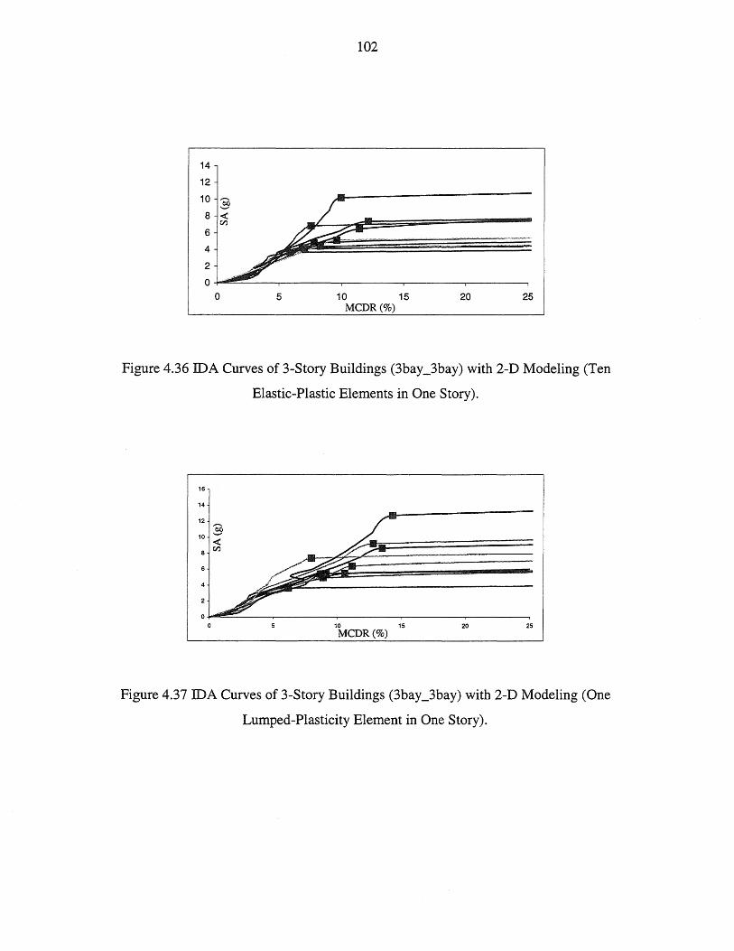
14
12
10
6
4
2
102
O~==----~------~----~------~------~
o 5 10 15 20 25 MCDR(%)
Figure 4.36 IDA Curves of 3-Story Buildings (3bay_3bay) with 2-D Modeling (Ten
Elastic-Plastic Elements in One Story).
16
14
10 15 20 25 MCDR(%)
Figure 4.37 IDA Curves of 3-Story Buildings (3bay_3bay) with 2-D Modeling (One
Lumped-Plasticity Element in One Story).
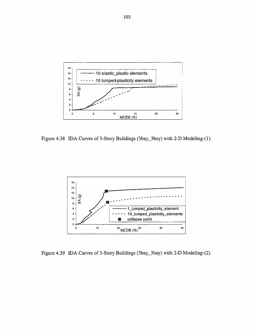
103
16
14 10 elastic_plastic elements 12
10 lumped-plasticity elements 10 .......... - ..... 8 ..... ~ 6
4
2
0 0 5 10 15 20 25
MCDR(%)
Figure 4.38 IDA Curves of 3-Story Buildings (3bay_3bay) with 2-D Modeling-(l).
16
14
12
o 10
11. •• --""-.- ... -----------
.. III III ..
---1_lumped-plasticity _element 1 O_lumped-plasticity _elements
• collapse point
20 MCDR (%) 30 40 50
Figure 4.39 IDA Curves of 3-Story Buildings (3bay _3bay) with 2-D Modeling-(2).
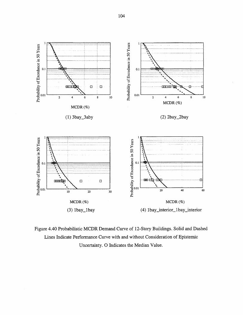
t+-< o
~ :§ .g 0.01
P::
MCDR(%)
... \-.... ~ ................................................................... " ........................................... · .. · .... ·1 .......... """""'''6'''''''''''''' ........ i ..... " ...... " .............................................................................. · .. · .. " ........ 1 ,
'" 0JIl[]IIlijm , ...
'" . 'i 10
o
20
MCDR(%)
(3) 1bay_1bay
o
30
104
0.1 .. """"""""":":':':::':::: ..... S;:::::: .. ............... \. .... .
................................. ......... , ....... .. .. ....... , ............ · ................................................ ·,· .. · .. · .... · .............. ·1
... .. ~ ............... " .......................................... .
" .............................. """O[ElEID~':'
" " 0.01 L....-_______ ---::lL....-...,;...,,;:._--'
6 8 10
Cf.l
~
~ o V)
.5 ~ u
2 4
MCDR(%)
(2) 2bay _2bay
§ 0.1 ~~====::::=====::::===::::=====::==j -g ............ \ ...... \-................................................................................ 0............................................ ..I
u ................ ~ .. .. >< ,
60
~ , t+-< ' o ' ~ ........ crm"dY.'~"'" .
" :§0.Q1 '" ..0 20 40
£ MCDR(%)
(4) 1 bay _interior_l bay_interior
Figure 4.40 Probabilistic MCDR Demand Curve of 12-Story Buildings. Solid and Dashed
Lines Indicate Performance Curve with and without Consideration of Epistemic
Uncertainty. 0 Indicates the Median Value.
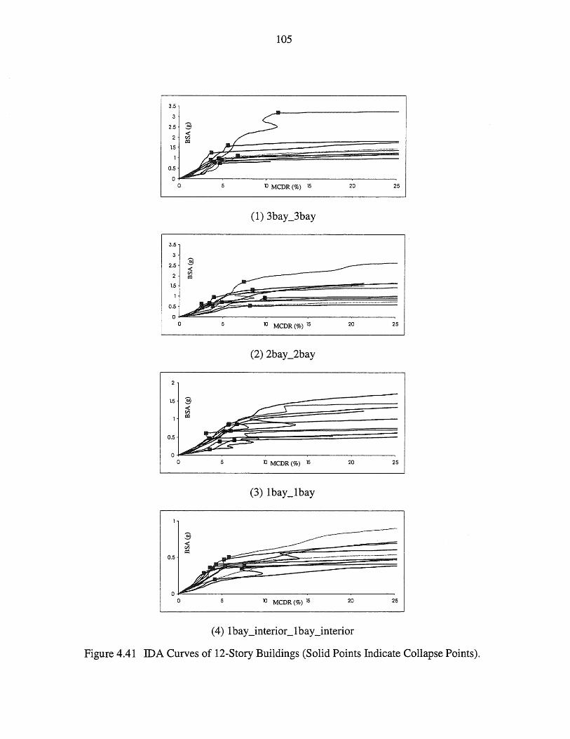
':1 2.5 §
2 < IZl ~
1.5
0.5
0 0
3.5
3
2.5 § <: IZl ~
1.5
0.5
0 0
1.5 § < IZl ~
0.5
105
... .-.... " .... """ .................... .... _--_ ...
D MCDR(%) 15 20 25
(1) 3bay_3bay
--.... ~-~.---.. .-.....
10 MCDR(%) 15 20 25
(2) 2bay _2bay
o~=---~------~------~------------~ o 5 D MCDR(%) 15 20 25
0.5 ---.-....... -~.-.. ~-
10 MCDR (%) 15 20 25
Figure 4.41 IDA Curves of 12-Story Buildings (Solid Points Indicate Collapse Points).

6@20f = 120 ft
6@30ft = 180 ft
_. '" ·
· · ..
. ...
." l-
· · ·
· · · I
· .... -
· B
.. ....
-p. -I-
..... .... · ·
· I
.... ool ..
"'1" ool ..
.. '" • 100
· . ·
106
9@20ft=180 ft
· · . ... . ,. · . .... .. I- .. .. · .. I- -I- ool .. · · · ~
ap. .1- .... .. I- -l- ."
'" . .. i- '"I'" ..I'" -;!~ .... ooll.
· • .1 · · 11""11
9@ 30 ft=270 ft
· .. ... · . . .... .... "1""-
ool .. .... ool .. .
"I- -'" .... .... • 100 .. .. · · .... -'" .... .... .~ .... ·
· R _JI . . . 1""1
Figure 4.42 The Plan View of Two Basic Configurations, 120'X180' (upper) and
180'X270' (lower).
40
30 :0-u e 20 -= ~ ~ u 10 c';S
]. is
0
0 5 10 15 20
Time (Second)
Figure 4.43 Time History of the 2-D Roof Displacement of IBC2000 3-Story Buildings
with Ductile Connections and Floor Area of 120'x180' and 180'x270'.
107
CHAPTER 5 RELIABILITY AND REDUNDANCY
5.1 Introduction
Structural reliability can be described in terms of system demand versus system
capacity. In this study, the maximum column drift ratio (MCDR) and the biaxial spectral
acceleration (BSA) are used to measure both system demand and capacity. Both aleatory
and epistemic uncertainties in the demand and capacity are considered.
The system demand in terms of MCDR is determined by performing a suite of time
history analyses of the response under the SAC ground motions. Alternatively, the system
demand can be also described in terms of BSA at the fundamental period corresponding
to the desired probability level. The system capacity in terms of MCDR or BSA is
determined by performing an IDA as described in the section 3.7.3.
Limit state probability analysis, fragility analysis, and redundancy analysis are
carried out using the system demand and system capacity statistics obtained and
described in Chapter 4. For a given building, the limit state probability can be expressed
as follows:
P[LS]= J p(LSID = d)fD(d)dd (5.1)
where D is a random variable describing the system demand, and P(LSID=d) is the
conditional limit state probability, given D = d, or the fragility curve. fo(d) is the density
function of D. The fragility curve is, therefore, a function of the capacity of the system
and its uncertainty.
As mentioned in section 1.1, although the benefit of redundancy in structural
system has been recognized for a long time, the redundancy concept has only begun to be
implemented into the design practice. Wang and Wen (2000) proposed a uniform-risk
redundancy factor, RR' for design to achieve a uniform reliability level for buildings of

108
different redundancies. In addition, this factor can be also used to evaluate the
redundancy of a given structural system. Hence, the RR factor, described in section 5.4.1,
is used in this study. The target (allowable) probability of incipient collapse is assumed to
be 2% in 50 years. The required design force is multiplied by a factor of 1IRR to achieve
the same reliability against incipient collapse for buildings of different
reliabili ty /redundancies.
A reliability/redundancy factor, p, was introduced in NEHRP 97, UBC 1997, and
mc 2000. This factor lacks sound theoretical basis. It can lead to undesirable designs and
has received criticism from the professions (e.g. Searer G. R. and Freeman S. A., 2002,
Wen and Song, 2003). Thus, a modified reliability/redundancy factor has been adopted in
NEHRP 2003 and proposed in ASCE-7 recently.
The reliability/redundancy factor defined in NEHRP 97 and NEHRP 2003 are
discussed in section 5.2 and section 5.3. In section 5.4, structural redundancy evaluated
according to the RR factor is compared with structural redundancy based on NEHRP 97
and NEHRP 2003. In section 5.5, based on the concept of redundancy indicator for a
simple parallel system, the regression analyses of the 1IRR factor on MCDR are carried
out. In section 5.6, the appropriateness of different seismic intensity measures are
examined. In addition to the spectral acceleration at the first mode, this study considers
also that of the second mode in determining of the RR factor. Fragility analyses and the
limit state probability analyses of buildings are performed in section 5.7.
5.2 The ReIiabilitylRedundancy Factor in NEHRP 97
ATC-34 (1995) recognized redundancy as one of the three elements of the "R"
factor and introduced the redundancy effects in building design. In the report, the number
of vertical lines of moment frames was used to measure the redundancy of a building. In
ATC-34, if a structure with four vertical lines of moment frames is regarded as a
redundant structure, there is no penalty on its seismic design. Otherwise, there is a
109
penalty for a non-redundant structure up to 40% increase in design force when there are
only two vertical lines.
NEHRP97 and IBC2000 also adopted a reliability/redundancy factor, p, and used it
as a multiplier of the lateral design earthquake load. The factor p is defined in the codes
as:
in US customary units
in SI units (5.2)
in which AB is the ground floor area of structures in ft2 or m2; r max is the maximum
element-story shear ratio. Because this definition takes into account only the floor area
and the maximum element-story shear ratio, it lacks an adequate rationale and can lead to
a poor structural design (e.g. Searer G. R. and Freeman S. A., 2002). Furthermore, other
factors such as ductile versus brittle connection behavior, uncertainty in demand and
capacity, irregular configuration, biaxial and torsion effects all have significant influence
on the performance of buildings, and have not been considered in this factor. Further
research is therefore needed to develop a more rational redundancy factor that enables
structure designers to evaluate and design for the effect of redundancy under stochastic
loads.
In order to investigate the effects of floor area and story number on the redundancy
of buildings, buildings of equal floor aspect ratios and equal number of moment-resisting
frames, but with different floor areas and number of story, are used for analyses (section
4.10). The structural redundancies, based on NEHRP 97 and the uniform-risk redundancy
factor, are then compared. The floor area effect on the building redundancy is also
examined.

110
5.3 The NEHRP Proposa12 .. 1R (NEHRP 2003)
A new proposal (NEHRP Proposal 2-1R) to improve the redundancy factor in
NEHRP 97 was adopted into NEHRP 2003 and currently under review by ASCE-7. This
redundancy factor is either 1.0 or 1.3, depending on the structures being classified as
redundant or non-redundant. According to this proposal, a steel moment frame can be
considered as a redundant structure if the following criteria are met.
1. Each story of the steel frame should provide at least 35% of the designed base-
shear.
2. No irregular configuration in plan exists.
3. There should be at least two moment resisting bays in each direction.
If a building fails to meet these criteria above, the designer may either perform an
additional analysis to examine the qualification of the structural redundancy or assign a
redundancy factor 1.3 to the structure. The additional redundancy analyses suggested in
NEHRP 2003 are as follows:
1. The story strength of a structure with a single beam failure at both ends is
required to retain 67% of the story strength of a structure without any
component failure.
2. An extreme torsional irregularity is not allowed when a beam loses its moment
resistance.
As mentioned in section 5.1, the redundancy defined in NEHRP 97 only considers
two factors, the floor area and the maximum element-story shear ratio. This definition
seems to work well in certain buildings; however, there are situations where it can lead
designers to poor designs, as shown by Searer G. R. and Freeman S. A. (2002) and will
be shown in section 5.4.4. The new p factor in NEHRP 2003 attempts to take a more
mechanism-based approach; however, its uniform factor of 1.3 may still fail to account
for the configuration variation and potential for serious damage in poorly designed
structures. For this reason, in this study, nine different plan configurations used as
111
prototype structure in the NEHRP proposal are designed as shown in section 3.8.2. Their
reliability and redundancy are then examined. Results using the new p factor in NEHRP
2003 and the RR factor are compared.
5.4 Uniform .. Risk Redundancy Factor
Wang and Wen (2000) introduced a uniform-risk redundancy factor, RR, for design
to achieve a uniform reliability level for buildings of different redundancies. This factor
can be also used to evaluate the redundancy of a given structural system. The RR factor is
defined as the ratio of spectral acceleration causing incipient collapse of a given structure
to that corresponding to an allowable probability. The RR factor is defined as follows:
[
1 when ~c ~ ~;ll R = Sic R S:ll when ~c ~ ~;ll
a
(5.3)
where ~c denotes the actual probability of incipient collapse; ~;ll denotes the
allowable probability of incipient collapse; and S!C and S:ll represent the elastic spectral
acceleration at the fundamental period causing incipient collapse at these two probability
levels. The elastic spectral acceleration at the fundamental period has been used as a
seismic hazard intensity measure in earthquake engineering. It is suitable when a 2-D
model is used to perform a structural analysis. This study focuses on a 3-D structural
response under biaxial excitations in which the interactions between responses in the two
principal directions and torsional motion are important. Thus, a more general ground
motion intensity measure is needed to take the 3-D effects into account. Wang and Wen
(2000) found the biaxial spectral acceleration (BSA) to be such a measure when biaxial
response is considered. BSA, defined as the maximum value of the vector sum of the
accelerations in the two orthogonal directions throughout time history analysis, is then
used in this study.
112
5.4.1 Methods of Determining the Uniform-Risk Redundancy Factor
As shown above, determining the RR factor requires the spectral acceleration
corresponding to an allowable probability of incipient collapse (S;ll) and the spectral
acceleration causing incipient collapse (S ~C). Wang and Wen (2000) used MCDR to
measure structural response and calculate the RR factor. Their method is used in this
study. The displacement demand and spectral acceleration are related by a power law
(Cornell et aI, 2002) as follows:
(5.4)
in which D is MCDR and Sa denotes the spectral acceleration. One can convert one
measure to the other using this relationship. For example, one can convert the
displacement capacity (Dc) on a given structure corresponding to the S!C and similarly,
the displacement demand (D) on a given structure corresponding to the S;ll , and vice
versa. The displacement demand (D d) is determined by performing a suite of time history
analyses of the response under SAC ground motions, and the results are given in section
4.8.1 and 4.9.1. The displacement capacity (DJ of a given structure against incipient
collapse is determined by performing IDA analyses. The results are shown in section
4.8.2 and section 4.9.2. Once Dc and Dd are obtained, the RR factor can be determined for
a given structure.
Shome and Cornell (2000) found that the dispersion of the displacement demand
(e.g. MCDR) at high intensity is very high (> 1.1). Therefore, the lognormal distribution
could fail to describe the distribution of the displacement demand. They proposed a three
parameters model to characterize the distribution of displacement demand, in which the
exceeding probability of a structure for a given intensity considers the "collapse" and "no
collapse" separately by using conditional probability. In view of high dispersion of
MCDR at high intensity, an alternative method of determining RR factor is proposed in
this study. The RR factor is determined using the S!C obtained directly at the collapse
113
point of each single IDA curve without going through the regression analyses. The S:ll
can be determined by using the spectral acceleration corresponding to the desired
probability level for the collapse prevention. Thus, following equation 5.3, the RR factor
can be detenuined. The advantages of using this method are:
1. Avoiding the possible regression analysis errors in the power law relationship.
2. Avoiding the much larger scatter in the MCDR demand. Because of the
softening load-displacement relationship observed in IDA curves, the transition
point is less sensitive when Sa is used. Table 4.5 displays the system demand of
3-story buildings in tenus of the MCDR. The COVs of the system demand vary
from 0.4 to 2.17, which is similar to the observation of Shome and Cornell
(2000). On the other hand, Table 5.2 displays the system demand of the same
buildings in tenus of the BSA. The COY s of the system demand vary from 0.2
to 0.37. Results shown here indicate that using BSA as the response measure
can effectively narrow the randomness of the system demand.
Both methods are used to construct the RR factor for comparison, and their results
are presented in the following sections.
5.4.2 Comparison of Results of 3-Story Buildings
The nine buildings of different plan configuration investigated in chapter 4 are used
again here for redundancy evaluations. Table 5.1 shows RR factors of these nine
buildings, in which the MCDR is used to measure system demand and system capacity.
The results above reveal an obvious tendency - buildings with more moment frames will
have a larger RR factor, hence, more system redundancy. As mentioned in section 5.4.1,
system demand and system capacity can be described in tenus of biaxial spectral
acceleration (BSA) as well. Table 5.2 and Table 5.3 provide the results of system demand
and system capacity analyses of these buildings using BSA. From the results above
(Table 5.2 and Table 5.3), the RR factors are constructed for each building, and their
results are shown in Table 5.4.

114
Comparing the results from Table 5.1 and Table 5.4, the trends of RR factor
determined by two different methods are similar. Further, the smaller the RR factor, the
bigger the difference between two methods. Since the MCDR is more sensitive to the
instability point in the IDA curves, consequently, when the MCDR is used as the
response measure, a large scatter in system demand is expected. As a result, more
dispersion is involved in the RR factor. This explains the difference in results shown in
Table 5.1 and Table 5.4. Since results shown here indicate that using BSA can reduce
scatter in system demand and dispersion in the RR factor calculation, the BSA is used in
constructing the RR factor in the following sections.
Figure 5.1 shows the results of 1IRR factors of these nine buildings, and Figure 5.2
provides the corresponding results of the redundancy factor (p) of these nine buildings
based on the NEHRP 2003. The p factor fails to prevent potential serious damage in non
redundancy structures, particularly for poorly designed structures. For example, the
previous analysis results displayed in section 4.2.1 and section 4.2.2 show that the design
of the 1 bay _interior_1 bay_interior building is not adequate to resist the seismic excitation,
and its response, represented by MCDR, is much larger than other buildings. However,
the penalty is 1.3 and equal to all other non-redundant buildings based on the p factor in
NEHRP 2003. Obvious, there is room for improvement in this method.
5.4.3 Comparison of Results of 12-Story Buildings
Wang and Wen (2000) only applied the uniform-risk redundancy factor (RR) to
low-rise steel frames. The suitability of the RR factor for mid-rise or high-rise steel frames
remains unclear. Therefore, the nine 12-story buildings of different plan configurations
analyzed in Chapter 4 are used again for redundancy analyses, and the uniform-risk
redundancy factor (RR) is evaluated for its suitability for mid-rise steel frames.
Table 5.5 and Table 5.6 show the system demand and system capacity of these nine
buildings, in which the BSA is used as the response measure. Table 5.7 shows the results
of the RR factor for these nine buildings. Again, buildings with more moment frames have
a larger RR factor. Figure 5.3 shows the results of 1IRR factors for these nine buildings.
115
The relationship between the number of moment frames and RR factors is similar to the
results of 3-story buildings. The 1IRR factor of the 12-story building is a little larger than
that of the 3-story building even though they have identical configuration. The
dependence of llRR factor on number of moment frames and number of story will be
investigated in a regression analysis in 5.5.
5.4.4 Redundancy as Function of Floor Area
The purpose of this section is to investigate the suitability of the p factor in NEHRP
97 and other current code, e.g. mc 2000. The buildings of equal floor aspect and equal
number of moment-resisting frames but different floor areas designed in section 4.10 are
used here for the redundancy analysis. According to the IDA results of steel frames of 3
to 20 stories (Wang, 1998), the drift ratio capacity against incipient collapse of steel
buildings without connection failures ranges from 7 to 10%. In the following calculation
of this section, drift ratio for incipient collapse of structures neglecting connection
failures is assumed to be 8%. The MCDR is used to calculate the RR. The MCDR is
assumed to be a log-normal distributed at each hazard level. The median MCDR
responses are multiplied by the correction factor to include the capacity uncertainty at the
two hazard levels, which allows for the determination of the probabilistic drift demand
curve. The probabilistic drift demand curve, as shown in section 4.10, is obtained for
each building and used to calculate the uniform-risk redundancy factor RR for each
building. The target ( allowable) probability of incipient collapse is assumed to be 2 % in
50 years for the overall system.
The RR and p factors are generally different for different buildings and can lead to
very different required base-shear design forces. Table 5.8 shows the differences in the
design forces based on the p factor compared with the uniform-risk redundancy factor
(RR). It is clear that the floor area does not affect the building redundancy as implied in
the p factor.
116
5.5 Regression Analysis of the Uniform-Risk Redundancy Factors
From the analysis results in section 5.4, uniform-risk redundancy factors (RR) are
obtained. It is of interest to investigate whether these factors can be described by
important structural configuration attributes such as number of moment frames and
number of stories. In reviewing of a simple parallel ductile system under static load, the
redundancy, defined as the ratio of the reliability index of a component to that of a
system, is a function of square root of the number of components. Regression analysis of
the RR factor on the number of moment frames and story number, therefore, takes the
following form
(5.5)
in which Y represents the inverse of the RR factor. Xl represents the number of
moment frames in a structure, and X2 represents the story number of a structure since
structural redundancy drops slightly as number of story increases as found in section
5.4.3. ~i denotes the coefficients of Xi'
The regression line expresses the best prediction (or estimation) of the dependent
variable (Y), given the independent variables (X). Several statistical methods are used to
evaluate whether the regression model fits the data well, and they are described in
Appendix B.
The proposed regression model (equation 5.5) giving the following relationship:
1 Y = 0.251 + 1.6396 r:v + 0.03X 2
VXl (5.6)
Regression statistics are shown in Table 5.9. The R-squared is 0.82, indicating that
82% of the original variability is explained by this model. The p-value of ~l variable is
very small (3.6E-8), which means the NH (null hypothesis) is rejected. In other words,
the variable, Xl' should not be removed from this regression model. The p-value of ~2
variable (0.00412) is not as small as that of the variable ~1' but it is still considered as a
117
small value compared to a common value of the significant level, 0.05. Therefore, the
variable X2 is kept in the regression model at this time. Figure 5.4 shows the plot of the
residuals and the Q-Q plot. From the residuals plot, no apparent pattern is observed and
thus no change of form of the regression equation is needed. According to the Q-Q plot,
data points form an approximate straight line indicating that the residual values follow
the normal distribution.
To investigate the effect of the story number, a new regression model is used, in
which the X 2 variable is removed. The result of the analysis is
1 Y = 0.473 + 1.6396 rv
VXl (5.7)
Table 5.10 shows the regression statistics, and Figure 5.5 shows the plot of the
residuals and the Q-Q plot. The value of the R-squared reduces from 0.82 to 0.65. There
is no apparent pattern on the plot of residuals. The Q-Q plot also indicates that the
residual values follow normal distribution. Based on the results, X2 only has a moderate
effect on the regression results. Additionally, Table 5.11 displays the regression results
for 3-story buildings from equation 5.6 and equation 5.7, and there is no significant
difference between them. As a result, number of story has only a moderate influence on
the building redundancy. Therefore, both regression models, equation 5.6 and equation
5.7, are considered to provide a good estimate of 1IRR as function of number of moment
frames and number of story and may be used as a guide in code provision.
5.6 Investigation of the Seismic Intensity Measures
This section investigates the efficiency of an alternative measure which is the sum
of spectral acceleration at the first and second modes, in conjunction with IDA. This new
measure may lead to a more accurate estimate of the uniform-risk redundancy factor.
As shown in section 5.4.1 and section 5.4.2, BSA is a better measure of demand on
structures for constructing the RR factor than MCDR. However, for a mid-rise or high-rise
steel frame, higher modes will have significant contribution on the overall structural
118
response as revealed in section 4.2. Luco and Cornell (2001) investigated six different
intensity measures (1M) of seismic hazard, including the elastic response of the first two
modes and the inelastic response of the first mode, using "efficiency" and "sufficiency"
as the criteria for selection of an intensity measure (1M). Efficiency denotes a small level
of the uncertainty in demand measure (e.g. drift response) for a given intensity measure.
Sufficiency denotes the independence of the demand measure on other parameters of
ground motion, such as magnitude and distance. Luco and Cornell found that the elastic
spectral acceleration or displacement at the fundamental period does not necessarily
satisfy these two criteria. This is especially true for taller buildings or buildings with long
periods where the seismic response is predominantly governed by higher modes.
In order to investigate the effects of the higher mode on the overall response and the
RR factor of mid-rise steel frames, a combination of the spectral acceleration of the first
two modes of the 12-story steel frames, analyzed in section 4.9, is proposed as follows:
SBSA = BSAjirstmode + BSAsecondmode (5.8)
in which, BSAfirsunode and BSAsecondmode represent the BSA at the fundamental period
and at the second period of the structure, respectively. A good ground motion intensity
measure should be a good prediction of the structural response, i.e. MCDR. The power
law, discussed in section 5.4.1, is used to describe the relationship between MCDR and
BSA as well as MCDR and SBSA for comparison. Figure 5.6 shows the regression plots
of MCDR on BSA, and Figure 5.7 shows the regression plots of MCDR on SBSA for the
12-story buildings. It is rather difficult to discern which measure describes the MCDR
better. Therefore, the R-squared value described in section Appendix B is used for this
purpose. Table 5.12 shows the R -squared value for each plot above. The results indicate
that including the BSA at the second period can improve the prediction of the structural
response for a taller building with a long period, however, the scatter of the MCDR are
still large (the R-squared is below 0.5 for all cases).
Table 5.13 and Table 5.14 show the results of system demand and system capacity
analysis of 12-story buildings in terms of SBSA, respectively. Based on these results, the
RR factor (and lIRR), in which the SBSA is used, can be constructed, as shown in Table

119
5.15. The results show a similar trend observed in the results using BSA. However, the
RR factor is smaller in some buildings, e.g., the 1 bay _interior_1 bay_interior building
(from 1.69 to 1.37). The method of regression analysis described in section 5.5 is used
here to establish the relationship between the RR factor and the number of moment
frames. The regression line is obtained as follows:
1 Y = 0.5848 + 1.2124 rv
VXl (5.9)
in which, Y = 11RR. Xl = the number of moment frames. Table 5.16 lists the
predicted values of 1IRR factors based on equations 5.7 and 5.9. The difference is
insignificant except when the number of moment frames is small. Both results indicate
that the lower bound of the total number of moment frames for a redundant building
should be not less than 10. In other words, for a moment frame system (perimeter) with
an identical number of moment bays in each direction, at least three moment bays in one
frame are needed to ensure the redundancy of a building against incipient collapse.
5.7 Fragility Analyses and the Limit State Probability Analyses
Three major elements are required to determine the fragility curve of a structural
system: ground motion intensity, system demand and system capacity. Previous sections
discussed the processes for determining these three elements. Based on the previous
results, the fragility and limit state probability of a structural system against incipient
collapse is analyzed in this section.
As described in section 5.1, for a given building, the limit state probability exposed
to a hazard can be expressed as follows:
P[LS]= J p(LSID = d)fD(d)dd (5.10)
where D is a random variable describing the system demand, and P(LSID=d) is the
conditional limit state probability, given D = d, or the fragility curve. The hazard is
defined by the probability fD(d), which is the density function of D. For evaluations of
120
building fragility under earthquake excitations, the system demand is represented by
spectral acceleration at the fundamental period of the building, consistent with the
specifications of seismic risk in a number of current codes, e.g., IBe2000.
Assuming lognormal distribution for system demand and capacity, the fragility of a
structural system can be described by a lognormal cumulative distribution function as
follows:
(5.11)
in which
<l> = standard normal probability integral
Ac represents the logarithmic mean of the system capacity
AD represents the logarithmic mean of the system demand
s c represents the logarithmic standard deviation of the system capacity
S D represents the logarithmic standard deviation of the system demand
The fragility curve of a structural system is therefore a function of the demand and
the capacity of the system and their uncertainty. Figure 5.8 and Figure 5.9 show the
fragility curves of 3-story buildings and 12-story buildings designed in section 3.8.2. As
expected, a building with more moment frames has a better performance, and therefore
can resist more severe earthquake excitation. Table 5.17 shows the 50-year incipient
collapse probability of the same 3-story buildings and 12-story buildings against incipient
collapse. The results are similar to the results of the fragility curves. Notice that the 50-
year limit state probability exceeds 20% for the building with only one moment frame in
each direction, and this holds true for both 3-story and 12-story buildings. This indicates
that a building with only one moment bay in the seismic excitation direction is a poor
design.

121
5.8 Tables
Table 5.1 Unifonn-Risk Redundancy Factors (RR) and Corresponding p Factors (lIRR) of 3-Story Buildings (using MCDR).
Building Type RR p (lIRR) P (NEHRP2003, under
Excitation in one Direction)
3bay_3bay 1 1 1
2bay_2bay 1 1 1
Ibay_lbay 0.792 1.26 1.3
3bay_lbay 1 1 1
2bay_lbay 1 1 1
3bay _1 bay_interior 0.61 1.64 1
2bay _1 bay_interior 0.79 1.27 1.3
1 bay _1 bay_interior 0.473 2.11 1.3
Ibay_interior_lbay_interior 0.414 2.41 1.3
Table 5.2 Statistics of Demand on 3-Story Buildings in Terms of BSA.
Hazard Level 10/50 2/50
Build Type Median (g) COY Median (g) COY
3bay_3bay 1.37 0.32 2.51 0.35
2bay_2bay 1.29 0.29 2.34 0.34
Ibay_lbay 1.18 0.25 2.14 0.35
3bay_lbay 1.27 0.34 2.42 0.37
2bay_lbay 1.23 0.28 2.34 0.35
3bay _1 bay_interior 1.14 0.32 2.08 0.2
2bay _1 bay_interior 1.1 0.23 1.81 0.33
1 bay _1 bay_interior 1.05 0.27 1.66 0.34
1 bay _interior_l bay_interior 0.66 0.44 1.06 0.31
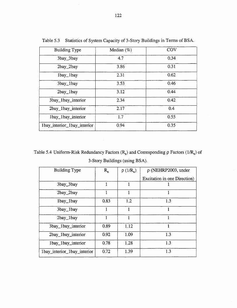
122
Table 5.3 Statistics of System Capacity of 3-Story Buildings in Terms of BSA.
Building Type Median (%) COY
3bay_3bay 4.7 0.34
2bay_2bay 3.86 0.31
Ibay_lbay 2.31 0.62
3bay_lbay 3.53 0.46
2bay_lbay 3.12 0.44
3bay _1 bay_interior 2.34 0.42
2bay _1 bay_interior 2.17 0.4
1 bay _1 bay_interior 1.7 0.55
1 bay _interior_l bay_interior 0.94 0.35
Table 5.4 Uniform-Risk Redundancy Factors (RR) and Corresponding p Factors (lIRR) of
3-Story Buildings (using BSA).
Building Type RR p (lIRR) p(~FU{P2003,under
Excitation in one Direction) 3bay_3bay 1 1 1
2bay_2bay 1 1 1
Ibay_1bay 0.83 1.2 1.3
3bay_lbay 1 1 1
2bay_lbay 1 1 1
3bay _1 bay_interior 0.89 1.12 1
2bay _1 bay_interior 0.92 1.09 1.3
1 bay _1 bay_interior 0.78 1.28 1.3
1 bay _interior_1 bay_interior 0.72 1.39 1.3
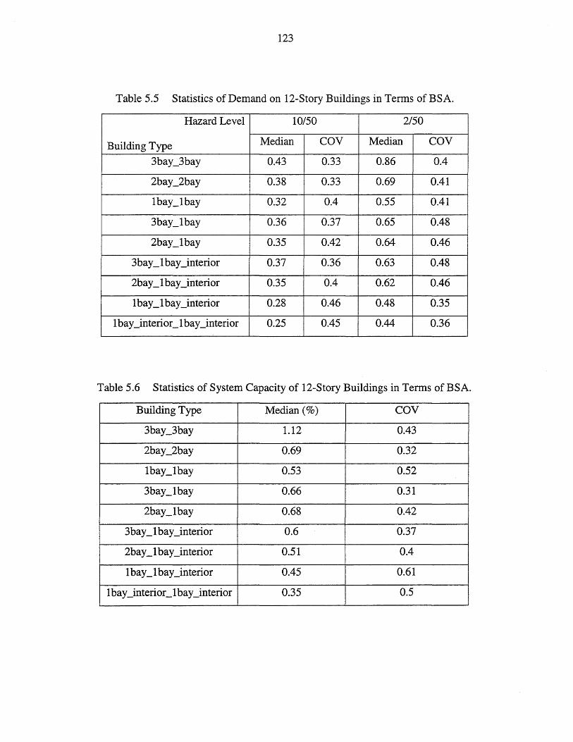
123
Table 5.5 Statistics of Demand on 12-Story Buildings in Terms of BSA.
Hazard Level 10/50 2/50
Building Type Median COY Median COY
3bay_3bay 0.43 0.33 0.86 0.4
2bay_2bay 0.38 0.33 0.69 0.41
1bay_1bay 0.32 0.4 0.55 0.41
3bay_1bay 0.36 0.37 0.65 0.48
2bay_1bay 0.35 0.42 0.64 0.46
3bay _1 bay_interior 0.37 0.36 0.63 0.48
2bay _1 bay_interior 0.35 0.4 0.62 0.46
1 bay _1 bay_interior 0.28 0.46 0.48 0.35
1 bay _interior_1 bay_interior 0.25 0.45 0.44 0.36
Table 5.6 Statistics of System Capacity of 12-Story Buildings in Terms of BSA.
Building Type Median (%) COY
3bay_3bay 1.12 0.43
2bay_2bay 0.69 0.32
1bay_1bay 0.53 0.52
3bay_1bay 0.66 0.31
2bay_1bay 0.68 0.42
3bay _1 bay_interior 0.6 0.37
2bay _1 bay_interior 0.51 0.4
1 bay _1 bay_interior 0.45 0.61
1 bay _interior_1 bay_interior 0.35 0.5

124
Table 5.7 Uniform-Risk Redundancy Factors (RR) and Corresponding p Factors (lIRR)
of 12-Story Buildings (using BSA).
Building Type RR p (lIRR) P (NEHRP2003, under
Excitation in one Direction) 3bay_3bay 1 1 1
2bay_2bay 0.87 1.15 1
Ibay_lbay 0.68 1.47 1.3
3bay_lbay 0.88 1.14 1
2bay_lbay 0.84 1.19 1
3bay _1 bay_interior 0.78 1.28 1
2bay _1 bay_interior 0.67 1.49 1.3
1 bay _1 bay_interior 0.6 1.67 1.3
1 bay _interior_l bay_interior 0.59 1.69 1.3
Table 5.8 Comparison of Uniform-Risk Redundancy Factor (RR) and p Factor
(defined NEHRP 97) of IBC2000 Buildings with Ductile Connections.
Buildings with Ductile Connections RR p
Story Number Floor Area Design Code
120X180' IBC2000 1 1.00 3-Story
180X270' IBC2000 1 1.26
120X180' IBC2000 1 1.00 12-Story
180X270' IBC2000 1 1.26
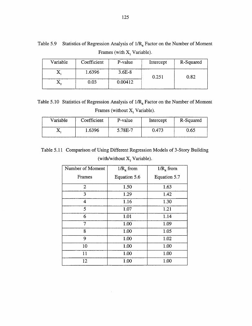
125
Table 5.9 Statistics of Regression Analysis of 1IRR Factor on the Number of Moment
Frames (with X2 Variable).
Variable Coefficient P-value Intercept R-Squared
Xl 1.6396 3.6E-8 0.251 0.82
~ 0.03 0.00412
Table 5.10 Statistics of Regression Analysis of 1IRR Factor on the Number of Moment
Frames (without X2 Variable).
Variable Coefficient P-value Intercept R-Squared
Xl 1.6396 5.78E-7 0.473 0.65
Table 5.11 Comparison of Using Different Regression Models of 3-Story Building
(with/without X2 Variable).
Number of Moment 1IRR from 1IRR from
Frames Equation 5.6 Equation 5.7
2 1.50 1.63
3 1.29 1.42
4 1.16 1.30
5 1.07 1.21
6 1.01 1.14
7 1.00 1.09
8 1.00 1.05
9 1.00 1.02
10 1.00 1.00
11 1.00 1.00
12 1.00 1.00
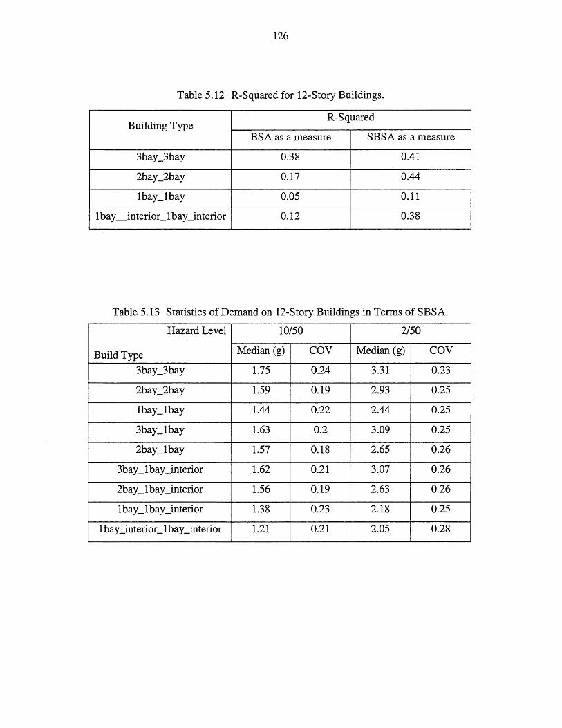
126
Table 5.12 R-Squared for 12-Story Buildings.
Building Type R-Squared
BSA as a measure SBSA as a measure
3bay_3bay 0.38 0.41
2bay_2bay 0.17 0.44
1bay_lbay 0.05 0.11
1 bay_interior_1 bay_interior 0.12 0.38
Table 5.13 Statistics of Demand on 12-Story Buildings in Terms of SBSA.
Hazard Level 10/50 2/50
Build Type Median (g) COY Median (g) COY
3bay_3bay 1.75 0.24 3.31 0.23
2bay_2bay 1.59 0.19 2.93 0.25
1bay_1bay 1.44 0.22 2.44 0.25
3bay_1bay 1.63 0.2 3.09 0.25
2bay_1bay 1.57 0.18 2.65 0.26
3bay _1 bay_interior 1.62 0.21 3.07 0.26
2bay _1 bay_interior 1.56 0.19 2.63 0.26
1 bay _1 bay_interior 1.38 0.23 2.18 0.25
1 bay _interior_1 bay_interior 1.21 0.21 2.05 0.28
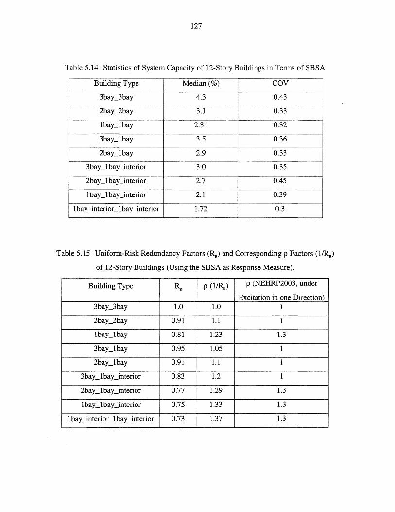
127
Table 5.14 Statistics of System Capacity of 12-Story Buildings in Terms of SBSA.
Building Type Median (%) COY
3 bay_3 bay 4.3 0.43
2bay_2bay 3.1 0.33
1bay_1bay 2.31 0.32
3bay_1bay 3.5 0.36
2bay_1bay 2.9 0.33
3bay _1 bay_interior 3.0 0.35
2bay _1 bay_interior 2.7 0.45
1 bay _1 bay_interior 2.1 0.39
1 bay _interior_1 bay_interior 1.72 0.3
Table 5.15 Uniform-Risk Redundancy Factors (RR) and Corresponding p Factors (lIRR)
of 12-Story Buildings (Using the SBSA as Response Measure).
Building Type RR p (lIRR) p(~f.lltP2003,under
Excitation in one Direction) 3bay_3bay 1.0 1.0 1
2bay_2bay 0.91 1.1 1
Ibay_1bay 0.81 1.23 1.3
3bay_1bay 0.95 1.05 1
2bay_1bay 0.91 1.1 1
3bay _1 bay_interior 0.83 1.2 1
2bay _1 bay_interior 0.77 1.29 1.3
1 bay _1 bay_interior 0.75 1.33 1.3
1 bay _interior_1 bay_interior 0.73 1.37 1.3
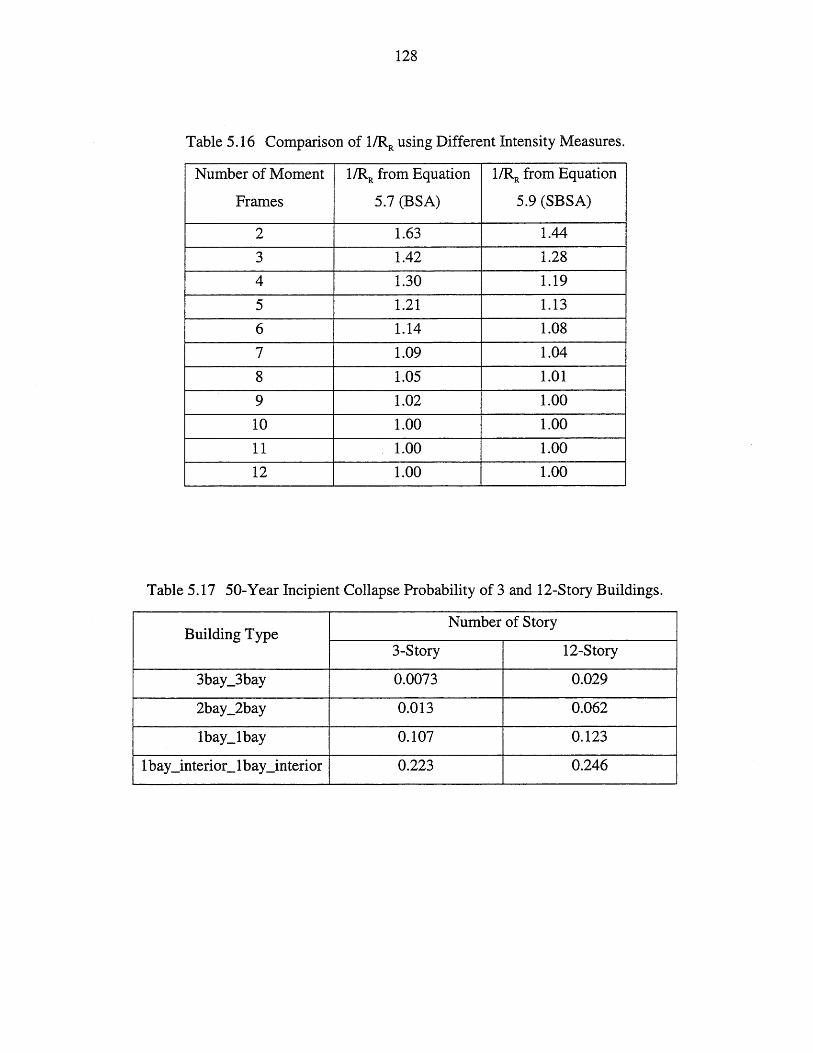
128
Table 5.16 Comparison of llRR using Different Intensity Measures.
Number of Moment llRR from Equation llRR from Equation
Frames 5.7 (BSA) 5.9 (SBSA)
2 1.63 1.44
3 1.42 1.28
4 1.30 1.19
5 1.21 1.13
6 1.14 1.08
7 1.09 1.04
8 1.05 1.01
9 1.02 1.00
10 1.00 1.00
11 1.00 1.00
12 1.00 1.00
Table 5.17 50-Year Incipient Collapse Probability of 3 and 12-Story Buildings.
Building Type Number of Story
3-Story 12-Story
3bay_3bay 0.0073 0.029
2bay_2bay 0.013 0.062
Ibay_lbay 0.107 0.123
1 bay _interior_l bay_interior 0.223 0.246
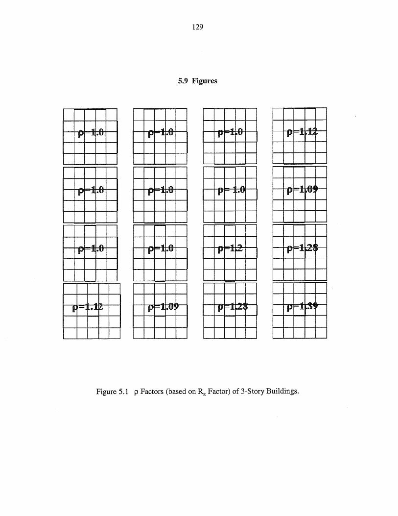
129
5.9 Figures
... .n. - ."111 n .... ,n, .... .... ... t' t-"-.1 .u t' '..I. aU p r--I ~'U' t' '..I. 1D..I...i:~
'iii ,n, - ..... .no .no - ."111 IlL ..
t' -.I .u t' '..I. .u p ;=0- J '-/IV t" '.I.. IRV::'
... .n. .41 on. - ..... """
.... ..... 111'"
t' .... .u t' 1"-..1 .u P 1-.1. ~ .. t' 1-.1. ~O
~- ........ .... .- .. ..-• - ", • .1. " p -<1 .u: , P ~.1. ~(~ P """:.1. IR"'~II'
[] I I I I
Figure 5.1 P Factors (based on RR Factor) of 3-Story Buildings.

130
....... -"f n ....... 1-111 n ."f ~ ~ 11 ~ p JIL aU p JIL .v P .JIL I-...JI! P" ..L ~1II.Ji'
....... -111 n ....... ,-11 n ....... -~ ~ 11 ~ p JIL IaV p JIL aU P fUJ P JIL II"'"
,11'1 n 11'1 n ,"f ~ - 11 ~ p JIL !tV p '..L leV P "..L .,.;po P "..L 1-.,)1'
""' ... - .... ..... ... -FJ' ..... u P -.I.. ~...:J P' ~.J. • .J P' ~.1.. ~~
Figure 5.2 P Factors (based on the NEHRP 2003) of 3-Story Buildings under Excitations in Y -Direction.

131
41 IlL - "111 --'It - .... ....... ~ t" " ... • u .... " .... ~ .I.;' t' '.I. ~CP
.... "" !or -II in. 'fit .dill ., r-.1 .. .I.~ l) tI 1-. ,,+ .... :;It tI " .... ;,"'Ir ..
'fit 'fit L11 - ""II 111111. - .111 ,j}lF, - .-111 ......... k' .,- " .. • .1. II' ., " ... • .I.~ t' -JI. p"'lr t' -..I. ..,U
""'" .... ~ "" A - .... , .. .-
~ -..I L~ ~ P ~.J. .'1:' P ~~ ~U p ;;;;:.1 ~O~,
Figure 5.3 P Factors (based on RR Factor) of 12-Story Buildings.
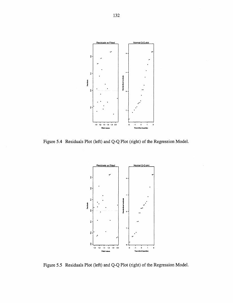
132
Residuals lIS Fitted Normal Q-Q olot
II·
d
~ ! i
c¥ oil
~ I
.. ~
":'
1.0 1.2 1.4 1.6 1.8 2.0 -2-1
Theoretical OJantilea
Figure 5.4 Residuals Plot (left) and Q-Q Plot (right) of the Regression Model.
"I • <;>
Residuals lIS Fitted
,..
2·
Normal Q-Q olot
,.
1.0 1.2 1.4 1.6 1.8 2.0 -2·1
Figure 5.5 Residuals Plot (left) and Q-Q Plot (right) of the Regression Model.
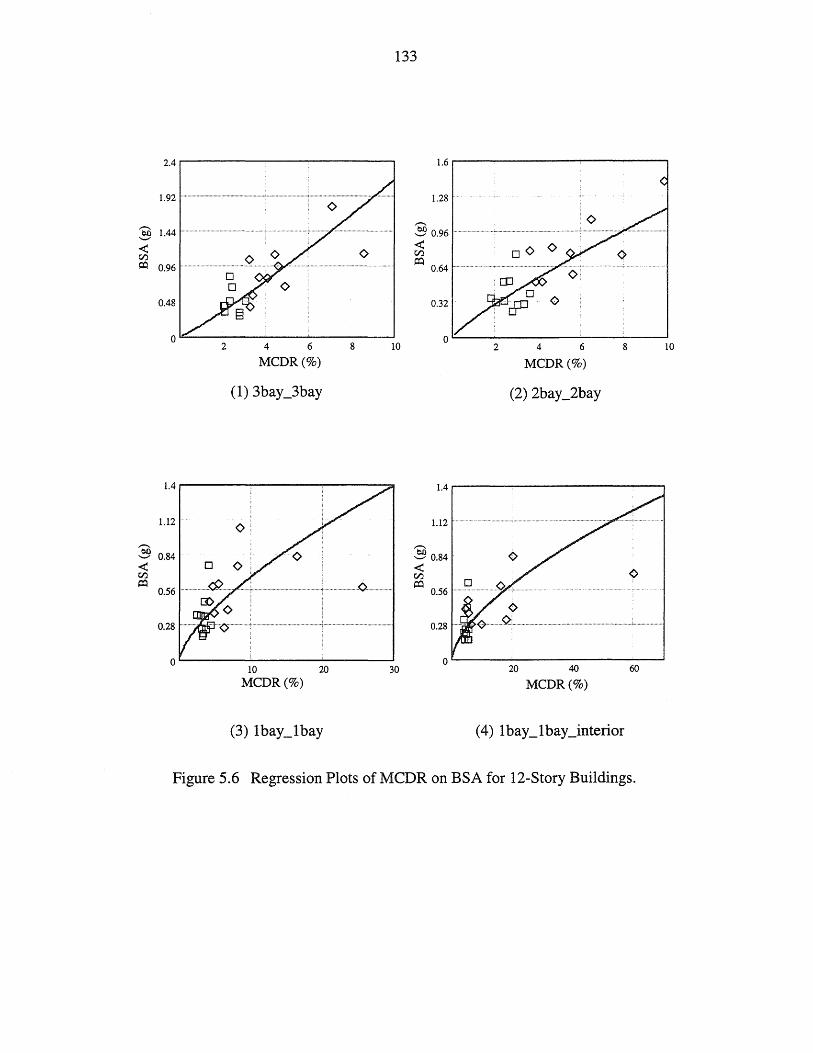
133
2.4 ....------....,.------------,
1. 92 I···· .. ····• .... · ...... · .................. · .. · ...... · .... ·· .. · ...... • .. ·· .... · ....................... ? ............................................... ;,I'-
bil 1.44 f ................................ · .... · ........................ , .. · ........................ · .. ··, ............. / ........
-< lZl ~ 0.96
0.48
o~-----~----~------~ 2 4 6 8 10
MCDR(%)
1.4 ....-----------....,.-----:::0
1.12
3 0.84 -< lZl ~
0.56
o~-----~------~----~ 10 20 30
MCDR(%)
1.6....---------.---------,
1.28
:§ 0.96 ...... <>
-< lZl
a::l 0.64 <>
0.32 <>
o~--~--------~--~--~ 2 4 6 8 10
MCDR(%)
1.4....----.......-----------.,
1.12 I· ................ · .... · .................... ·• ................ · ........ · .. · .. · .......... · .. ·· ....................... :.:..". ........ ,.......... · .. 1
:§ 0.84
-< ~ 0
0.56 .
0.28 ..
o~----~------------~~ 20 40 60
MCDR(%)
Figure 5.6 Regression Plots of MCDR on BSA for 12-Story Buildings.
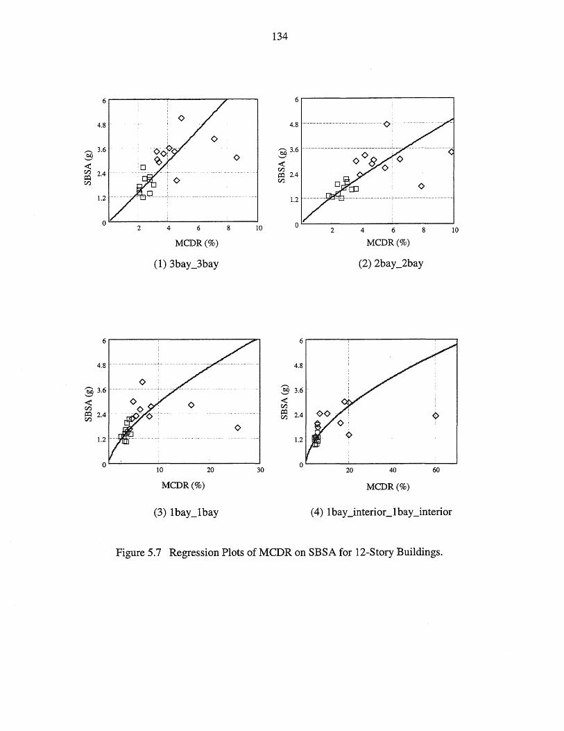
6
4.8
.......... 3.6 ~ <> -< CZl 2.4 ~ CZl
1.2
0 2 4 6 8 10
MCDR(%)
(1) 3bay _3bay
6~--------------~----~
-< CZl
4.8
~ 2.4 ... CZl
1.2 1 .............. = .... .
o~~--~--------------~ 10 20 30
MCDR(%)
134
6
4.8 ..
eo 3.6 '-"'
-< CZl ~ 2.4 CZl
<> 1.2
0 2 4 6 8 10
MCDR(%)
(2) 2bay _2bay
6~----~------------~~
4.8
:§ 3.6 .
-< CZl
B3 2.4
1.2
o~----~------------~~ 60 20 40
MCDR(%)
Figure 5.7 Regression Plots of MCDR on SBSA for 12-Story Buildings.

135
0.8
~ U·' a 0.6
13 ~ U ><
t:!l ....... 0.4 0
~ ~ .D 0 0.2 ....
0..
5 10 3bay _3bay BSA(g)
15
2bay_2bay 1 bay_l bay 1 bay _interiocl bay_interior
Figure 5.8 Incipient Collapse Fragility Curves of 3-Story Buildings.
0.8
~ U a ]
0.6 U ><
t:!l ....... 0
~ 0.4 ~ .D 8
0..
0.2
246 8 10 3 bay_3 bay SBSA(g) 2bay_2bay Ibay_lbay 1 bay _interioc 1 bay_interior
Figure 5.9 Incipient Collapse Fragility Curves of 12-Story Buildings.
136
CHAPTER 6 CONCLUSION AND RECOM:MENDATIONS
6.1 Conclusions
The benefit of structural redundancy has been long recognized, and a number of
researchers have investigated the positive effects of redundancy on overall structural
response. However, there is only limited implementation of the redundancy concept into
the structural design. This study focuses on the structural redundancy of steel moment
frames and the subsequent application of redundancy to engineering practices.
The reliability/redundancy factor, p, defined in NEHRP 97, UBC 1997, and IBe
2000, is used as a multiplier of the lateral design earthquake load. Because this factor
only considers the floor area and maximum element-story shear ratio, but not any of the
other important redundancy contributing factors, it can lead to poor structural designs.
Recently, a modified reliability/redundancy factor was proposed in NEHRP Proposal 2-
1R and adopted into NEHRP 2003. It is a more reasonable and mechanism-based
approach, and likely to be implemented in building codes in the near future. However, its
uniform penalty of increasing the lateral design force for non-redundancy structures
regardless of details in configuration is still debatable. For a structure system of
complicated nonlinear response behaviors and with high uncertainty in demand and
capacity, its redundancy can be measured meaningfully only in terms of reliability.
Therefore, a systematic probabilistic study of redundancy of steel moment frame system
was carried out and the uniform-risk redundancy factor was developed for assessment of
redundancy.
The inelastic behavior of connections has been shown to play an important role in
structural response and redundancy evaluation. The Bouc-W en smooth connection
fracture hysteresis model was used here to take the effects of brittle connection failures
137
into account. This model was then incorporated into the ABAQUS computer program as
a user-defined-element (VEL) to account for the inelastic and degrading connection
behavior of steel moment frames. In addition, the experimental results of connection
capacity, documented in FEMA 355D, were implemented in this VEL to consider
potential brittle connection behaviors and their variability. To account for the biaxial
interaction of buildings with non-uniform mass distribution or with asymmetric plan
configuration, a 3-D finite element model based on ABAQUS was developed in which
the lateral resistance of the gravity frames is also included. Other important factors
considered include: (1) uncertainties in material, (2) uncertainties in connection capacity,
(3) P-.6. effects, (4) panel zone effects, (5) inelastic column behaviors and (6) 5%
accidental torsion.
The evaluation of structural redundancy against incipient collapse was carried out
through a framework that considers: (1) the maximum column drift ratio (MCDR) and
biaxial spectral acceleration (BSA) as a measure of both the demand and the capacity of a
given building; (2) the demand and capacity using Incremental Dynamic Analysis (IDA)
of a building which yields the probabilistic demand curve and the distribution of capacity;
(3) both aleatory and epistemic uncertainties in demand and capacity; (4) the uniform-risk
redundancy factor, RRo RR factor was used in design to achieve a uniform reliability level
for buildings of different redundancies as well as to evaluate the redundancy of a given
structural system.
The p factor in NEHRP 97, in NEHRP 2003 and RR factor were compared.
Fragility curve and limit state probability analyses were also conducted, and the structural
reliability was examined.
Based on the numerical study of the reliability and redundancy of low-rise and mid
rise steel moment frames, the following conclusions are drawn:
1. Fractured beam-column connections may experience larger rotation and loss of
energy-dissipating capacity, resulting in larger responses of buildings. An
accurate modeling of the hysteretic behavior of fractured connection is
necessary for predicting the performance of steel frame buildings. The
138
proposed Bouc-W en smooth hysteresis model incorporated into ABAQUS
serves this purpose.
2. Fracture failure of the pre-Northridge connections had a more severe impact on
the building performance than that of post-Northridge connections. The results
shown in section 4.4 indicate that the median capacity of pre-Northridge
connections was only 80% of the median capacity of post-Northridge
connections.
3. As expected, the number of fractured beam-column connections and the overall
stability are interrelated. As the connection failure occurs progressively, the
overall performance deteriorated.
4. Panel zones have only a moderate influence on the overall response if the shear
strength is adequate.
5. The Strong Column Weak Beam (SCWB) design guideline cannot prevent the
development of plasticity in columns. To investigate the effect of inelastic
column behavior on structure performance, three different modeling techniques
were used in this study: elastic column, elastic-plastic column and lumped
plasticity column. The elastic-plastic model was found to have similar behavior
as the lumped-plasticity model and was used to simulate the column response
because it is closer to reality.
6. The first mode dominates only the response of low-rise steel frames. For mid
rise steel frames, higher modes may have a significant effect on the building
response.
7. Incremental dynamic analyses (IDA) determining the building capacity and its
uncertainty against incipient collapse were successfully extended to 3-D to
incorporate 3-D effects.
8. The number of moment frames has a significant impact on the demand on
structures in terms of MCDR. Buildings with more moment frames will have
139
smaller MCDR demand. However, it does not have a significant influence on
the system capacity in terms of MCDR against incipient collapse.
9. BSA was proven to be a better measure for demand and capacity against
incipient collapse than the MCDR when determining the RR factor. One of the
advantages of the BSA is avoiding the error in the power law regression
analysis required for the BSA and MCDR. The other benefit is that using BSA
can reduce the randomness of the system demand.
10. The combined spectral acceleration, SBSA, of both first and second modes of a
building, can predict the structural MCDR demand of mid-rise steel moment
frames more accurately than BSA.
11. The regression models proposed in this study are considered to provide a good
estimate of llRR as function of number of moment frames and number of story
and may be used as a guide in code provision. Results indicate that at least
three moment frames in each principal direction are needed to ensure a
structure with adequate redundancy.
12. The p factor in NEHRP 97 generally overestimates the effects of floor area
because of its failure to consider all other important redundancy-contributing
factors, e.g., the fracture behavior of beam-column connection, uncertainty in
demand and capacity, etc.
13. The p factor in NEHRP 2003 fails to capture the variations and potential for
serious damage for non-redundant and poorly designed structures. Buildings
with asymmetric plan configurations may experience a larger torsional
displacement and cause the building to lose the ability to resist excitations. The
new p factor generally underestimates this effect because of its failure to
consider the interaction between the motions in two principle directions of the
structures.
14. The results of the fragility and limit state probability analyses indicate that
buildings with a small number of moment frames are more likely to experience

140
incipient collapse therefore are more vulnerable under future seismic
excitations. They need to be strengthened according to the uniform-risk
redundancy factor to achieve the desired reliability level against incipient
collapse.
6.2 Recommendations for Future Research
The results of this study provide insight into the performance of three-dimensional
low-rise and mid-rise steel moment frames under seismic excitations. Some issues,
however, require further investigation:
1. This study uses the biaxial spectral acceleration (BSA or SBSA), determined
by the maximum value of the vector sum of the accelerations in the two
principal directions throughout the time history, to measure the intensity of
ground motion. However, its use is questionable when the first and second
modes of buildings are not in the two translation directions. Other measures are
needed for buildings with large torsional motions.
2. In this study, only the torsional effects due to unsymmetric failure of structure
members on symmetric buildings were investigated. Buildings of irregular
configuration (L or T shape in plan) were not considered. For irregular
buildings, the effects of torsion are expected to cause a more serious concern
and need further investigation.
3. The regression results of the p factor (lIRR) are valid only over the range of
values of the number of moment frames for which the data have been
investigated, e.g., from two moment bays to twelve moment bays. Strictly
speaking, it is not appropriate to apply this regression equation to a system
outside this range. Investigations of other plan configurations are needed to
obtain regression equation applicable to more general systems.
4. The Bouc-Wen smooth model used in this study takes only the uniaxial
connection response into account. The biaxial interactions of connections are

141
known to have effects on the overall response. The contribution of the biaxial
interactions of beam-column connections has not been considered. Their
influence needs further investigation.
5. The procedure for redundancy evaluation was for investigation of low-rise and
mid-rise steel moment frames. Applicability of this methodology to high-rise
steel moment frames requires further invest~gation.
6. Except the 1bay_interior_1bay_interior structure, investigation has been
conducted for perimeter moment frame systems in this study, yet other core
moment frame systems are also commonly used in the United States. It is of
interest to investigate and compare the response characteristics and redundancy
of the two different systems.
142
APPENDIX A SYSTEM REDUNDANCY OF SIMPLE PARALLEL SYSTEMS
Before the regression analysis of the uniform-risk redundancy factor (RR) is
conducted, system redundancy of a parallel system is briefly reviewed and a redundancy
indicator, Rind' is derived. Although the behavior of steel moment frames is not the same
as that of a parallel system, the redundancy indicator (Rind) depicts the system redundancy
for a parallel system well, and provides useful information such as the relationship
between the number of components and system redundancy. This relationship is assumed
to be true for steel moment frames. Therefore, the form of the redundancy indicator (Rind)
is then used as the basis to construct the formulation of the regression model (the form of
X). System redundancy of a parallel is described as follow.
Structural system in engineering is complicated and not easy to predict. Two simple
categories, series and parallel, are commonly used to make the complicated system ideal.
A series or weakest link system refers to a system, in which the failure probability of one
component is equal to the failure probability of the whole system, as shown in Figure
A.I. On the other hand, when one or more components reaching the limit state does not
necessarily indicate a system failure, the system is known as a parallel or redundant
system, as shown in Figure A.l. Mechanism differences between a parallel system with
brittle components and one with ductile components are significant.
The probability distribution of the safety margin for a component is Mj=Rj-Qj, in
which Rj is the ith component strength and Qj is the loading on the ith component. The
following assumptions are used to derive the redundancy of a parallel system:
1. Each component has ideal elastic-plastic behavior.
2. The load-sharing among components is perfectly equal and independent.
3. The strength of each component is independent.
System strength is then given as
143
n
R = "" R. s £... I (A. 1)
i=l
The total loading on the system is then given as
(A.2)
The safety margin of the system (M) is then given as
n
M =""M. s £... I (A.3)
i=l
in which n represents the number of components, M j is the safety margin of the ith
component. As one can see, Ms is a linear combination of several random variables. Its
mean and variance can be described as follows:
n n
E(M) = f.1M = LE(Mi ) = Lf.1Mj (A.4) i=l i=l
n n
E[(M - f.1M )2] = var(M) = LLPijO" MjO" Mj
(A.S) i=l j=l
where 0 Mj is the standard deviation of Mi and pij is the correlation coefficient
between Mi and Mj, with pii=l. The standard deviation of safety margin of the system
(as) can be obtained as follows:
n n
O"s = LLPijO"MjO"Mj i=l j=l
To simplify the derivation, the following conditions are made:
(A.6)
1. The strength of each component is identical and is a normal distributed random
variable.
2. The loading on each component is also a normal distributed random variable.
3. The correlation coefficient between Mi and Mj is identical (p ij = p) .
Equation (A.4) and equation (A.6) then can be reduced to
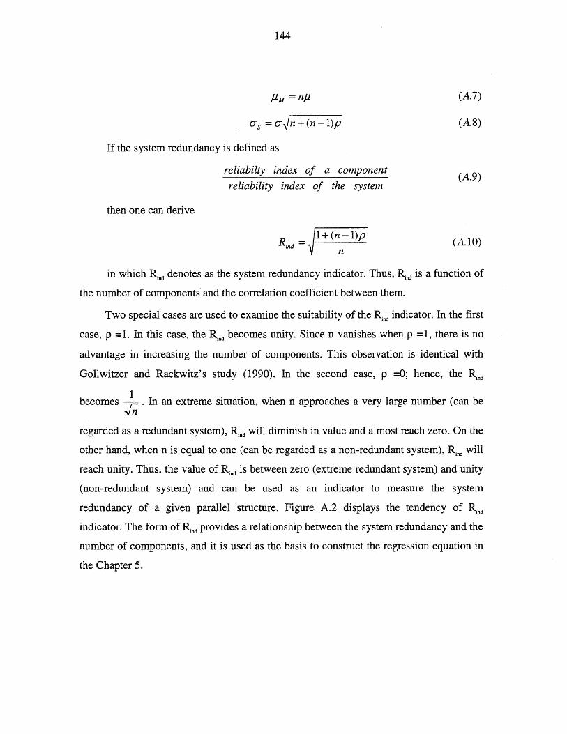
144
f.lM = nf.l
O"s =0"~n+(n-1)p
If the system redundancy is defined as
then one can derive
reliabilty index of a component
reliability index of the system
(A.7)
(A.S)
(A.9)
(A. 10)
in which Rind denotes as the system redundancy indicator. Thus, Rind is a function of
the number of components and the correlation coefficient between them.
Two special cases are used to examine the suitability of the Rind indicator. In the first
case, p =1. In this case, the Rind becomes unity. Since n vanishes when p =1, there is no
advantage in increasing the number of components. This observation is identical with
Gollwitzer and Rackwitz's study (1990). In the second case, p =0; hence, the Rind
becomes .);;. In an extreme situation, when n approaches a very large number (can be
regarded as a redundant system), Rind will diminish in value and almost reach zero. On the
other hand, when n is equal to one (can be regarded as a non-redundant system), Rind will
reach unity. Thus, the value of Rind is between zero (extreme redundant system) and unity
(non-redundant system) and can be used as an indicator to measure the system
redundancy of a given parallel structure. Figure A.2 displays the tendency of Rind
indicator. The form of Rind provides a relationship between the system redundancy and the
number of components, and it is used as the basis to construct the regression equation in
the Chapter 5.
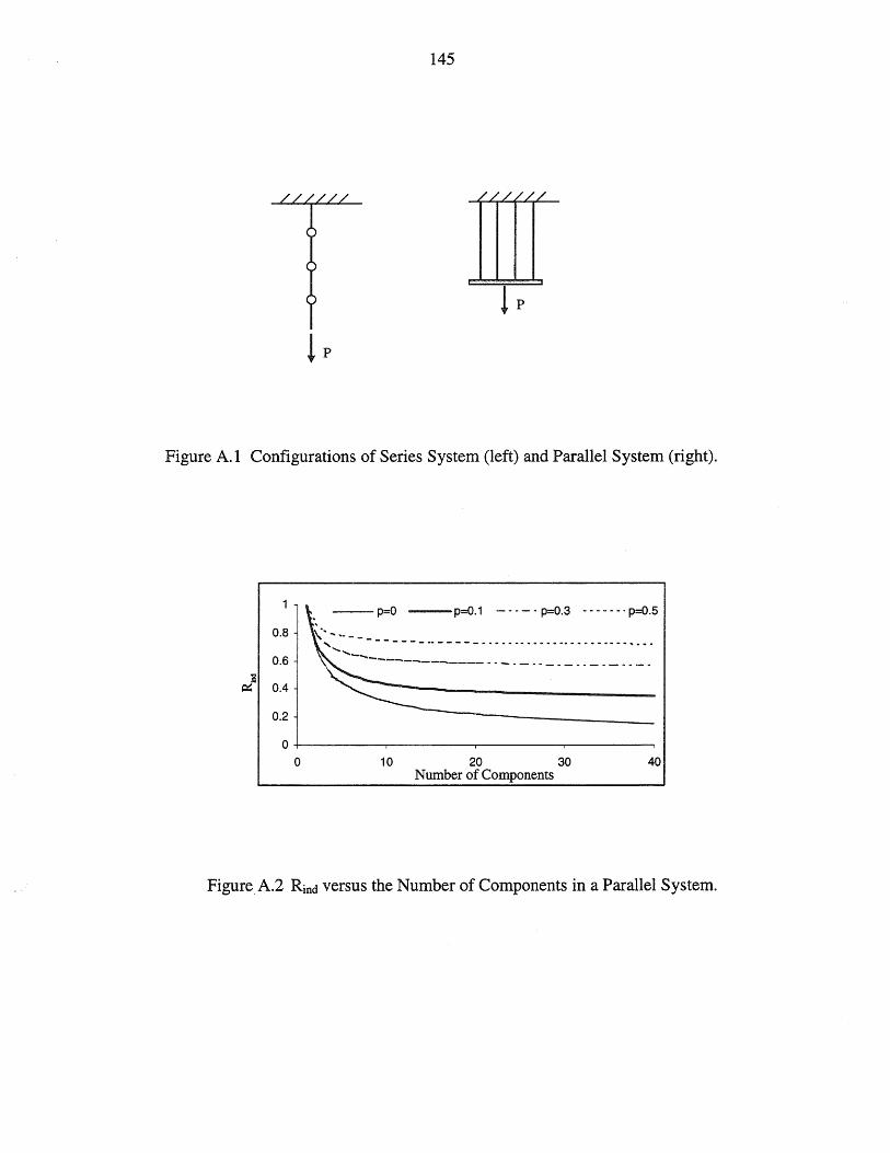
145
// //
Figure A.I Configurations of Series System (left) and Parallel System (right).
-- p=O --p=O.1 _.0 - 0 p=0.3 _.0 - - _. p=O.5
0.8
0.6
;\~ .. -. - - - - - - - - - 00 _____ • 0 ••••••• _ • __ •••••••••• _ •••
....... ,-....... -. ..... - ...... -----.._--_ .... - .. _ ..... _ ... _ .. -_ ... _ ..... _ ... ~"§ 0.4
0.2
0
0 10 20 30 40 Number of Components
Figure A.2 Rind versus the Number of Components in a Parallel System.
146
APPENDIX B STATISTICAL TEST AND RESIDUAL DIAGNOSIS
Methods used as evaluations in the regression analysis are listed and explained as
follows:
1. Residuals plot.
The deviation of an observed data from the regression line is called the residual
value. Once a plot of residuals versus fitted values is created, the shape of the plot is
observed. If a plot shows any certain tendency, it will be described as with a pattern.
Different transformations of variables are suggested based on different patterns of plots.
If there is no apparent pattern observed in the plot, the regression model (or regression
equation) is expected to be appropriate. More detail of residuals plot can be found in
Weisberg (1985).
2. The R-squared value.
The R-squared value represents how much variability of the original variability is
explained by the regression line. It is obvious, as the R -squared approaches unity; a
regression approaches a perfect fit. The mathematical formulation of the R-squared value
is
(B.l)
in which Y represents the value of a observed data, Y represents the value on the
regression line corresponding to Y, and Y represents the mean value of Y.
3. The p-value.
The probability value (p-value) of a statistical hypothesis test is the conditional
probability of observing a value of the computed statistic (here, the value of Pi) as
extreme or more extreme (here, as larger or larger) than the observed value, given that
null hypothesis (NH) is true. A small p-value provides evidence against NH (Weisberg,
1985). A statistical hypothesis is simply a statement about the numerical value of an
147
unknown parameter (Glass and Hopkins, 1996). The null hypothesis (NH) is a statement
that has been put forward, either because it is believed to be true or because it is used as a
basis for argument, but has not been proved. For example, in this study, the NH is that
there is no difference between the coefficient (~i) of the variables (Xi) and zero. If the p
value is small enough (i.e. <0.05) for a ~i, the NH is rejected. In other words, there is
significant evidence to support the existence of the variable Xi corresponding to the ~i.
4. Q-Q plots.
The Quantile-Quantile (Q-Q) plot is used to determine whether the two data sets
come from populations with a common distribution. If so, points on the plot should form
approximately a straight line. It is a common assumption that the residual values follow
normal distribution when the method of least squares is used. A theoretical distribution
(here, normal distribution) is then used as one of the data samples in the Q-Q plot, and
the residual variables are used as the other data samples. Thus, the distribution of the
residual variables is compared to the normal distribution by the Q-Q plot. It is interesting
to point out that once one of the data samples of the Q-Q plot are replaced by a
theoretical distribution, the Q-Q plot is similar to a probability plot (probability paper).
148
REFERENCES
ABAQUS Version 6.4 online Documentation, 2003.
AISC, "Seismic Provisions for Structural Steel Buildings." ANSIIAISC 341-02, 2002.
Ang, A., and Tang, W. "Probability Concepts in Engineering Planning and Design." Vol. 2, john Wiley & Sons, New York, 1984.
ATC-34, "A Critical Review of Current Approaches to Earthquake Resistant Design." Applied Technology Council, Redwood City, California, 1995.
Baber, Thomas T. and Noori, Mohammad N., "Random Vibration of Degrading, Pinching Systems." J. Engrg. Mechanics, ASCE, 111(8), pp. 1010-1017,1985.
Baber, Thomas T. and Wen, Yi-Kwei, "Random Vibration of Hysteretic, Degrading Systems." J. Engrg. Mechanics, ASCE, 107(EM6), pp. 1069-1074, 1981.
Bertero, R. D. and Bertero, V. V., "Redundancy in Earthquake-Resistant Design." J. Struct. Engrg., ASCE, 125(1), pp. 81-88, 1999.
Cornell, C. A., "Offshore structural systems reliability." Rep., C. Allin Cornell, Inc., Portola Valley, Calif., 1987.
Cornell, C. A., Fatemeh Jalayer, Hamburger, R. O. and Foutch, D. A., "Probabilistic Basis for 2000 SAC Federal Emergency Management Agency Steel moment Frame Guidelines." J. Struct. Engrg., ASCE, 128(4), pp. 526-533,2002.
De, R. S. and Cornell, C. A., "Offshore structural system reliability: wave-load modeling, system behavior, and analysis." Rep. No. RMS-6, Dept. of Civ. Engrg., Stanford Univ., Calif., 1990.
De, R. S., Karamchandani, A. and Cornell, C. A., "Study of Redundancy in Near-Ideal Parallel Structural Systems." ICOSSAR'89, Structural Safety and Reliability, pp. 975-982, 1989.
El-Tawil, S., Vidarsson, E., Mikesell, T. and Kunnath S. K., "Inelastic Behavior and Design of Steel Panel Zones." J. Struct. Engrg., ASCE, 125(2), pp. 183-193, 1999.
Foliente, Greg C., "Hysteresis Modeling of Wood Joints and Structural Systems." J. Struct. Engrg., ASCE, 121(6), pp. 1013-1017, 1995.
149
Foutch, D. A. and Shi, Shan, "Effects of Hysteresis Type on the Seismic Response of Buildings." 6th U. S. National Conference on Earthquake Engineering, Seattle, Washington, 1998.
FEMA-273, "NEHRP Guidelines for the Seismic Rehabilitation of Buildings." Federal Emergency Management Agency, Washington D. C., 1997.
FEMA-289, "Connection Test Summaries." Federal Emergency Management Agency, Washington D. C., 1997.
FEMA-302, "NEHRP Recommended Provisions for Seismic Regulations for New Buildings and Other Structures." Federal Emergency Management Agency, Washington D. C., 1998.
FEMA-355D, "State of Art Report on Connection Performance." Federal Emergency Management Agency, Washington D. C., 2000.
Glass, G. V. and Hopkins, K. D., "Statistical Methods in Education and Psychology." Third Edition, Allyn & Bacon, 1996.
Goel, R. K. and Chopra, A. K., "Vibration Properties of Buildings Determined from Recorded Earthquake Motions." Report No. UCBIEERC-97/14, University of California at Berkeley, December, 1997.
Gollwitzer, S. and Rackwitz, R, "On the Reliability of Daniels System," Structural Safety, Vol. 7, pp. 229-243, 1990.
Hendawi, S. and Frangopol, D. M., "System Reliability and Redundancy in Structural Design and Evaluation," Structural Safety, Vol. 16, pp. 47-71, 1994.
Hilber, H. M., T. J. R. Hughes, and R. L. Taylor, "Collocation, Dissipation and ... Overshoot' for Time Integration Schemes in Structural Dynamics." Earthquake Engineering and Structural Dynamics, vol. 6, pp. 99-117, 1978.
mc 2000, "International Building Code," BOCA, ICBO., 1998.
J ames, A Swanson, "Characterization of the Strength, Stiffness, and Ductility Behavior of T-stub Connections." PhD. Dissertation, Roberto Leon, faculty advisor, School of Civil & Environmental Engineering, Georgia Institute of Technology, Atlanta, 1999.
Kennedy, D. J. L. and Baker, K. A., "Resistance Factors for Steel Highway Bridges." Can. J. Civ. Eng., Ottawa, Vol. 11, pp. 324-334,1984.
Krawinkler, H., "Shear Design of Steel Frame Joints." Engineering Journal, AISC, Vol. 15, No.3, 1978.
150
Liao, K. W. and Wen, Y. K., "Performance Analysis of Essential Facilities in MidAmerica." 2th International Conference on Structural Stability and Dynamics, Singapore, 2002.
Liu, J. and Astaneh-AsI, A., "Cyclic Tests on Simple Connections Including Effects of the Slab." SAC Report No. SACIBD-00I03, 2000.
Luco, Nicolas and Cornell, C. A. "Structure-Specific Scalar Intensity Measures for NearSource and Ordinary Earthquake Ground Motions." Submitted for Publication: Earthquake Spectra, April 2001.
Maes, M. A., "Ignorance factors using model expansion," J. Engrg. Mech., ASCE, 122(1), pp. 39--45, 1996.
McGuire, William and Gallagher R. H., "Matrix Structural Analysis." John Wiley & Sons, 1979.
NEHRP 2003 (FEMA-450), "NEHRP Recommended Provisions for Seismic Regulations for New Buildings and Other Structures." Federal Emergency Management Agency, Washington D. C., 2004.
Parlett, B. N., "The Symmetric Eigenvalue Problem." Prentice-Hall, New York, 1980.
Saad, Y., "Numerical Methods for Large Eigenvalue Problems." John Wiley & Sons, 1992.
SAC 96-01, Part 1, "Technical Report: Experimental Investigations of Beam-Column Subassemblages," SAC Steel Project, Sacramento, California, March 1996.
SAC Background Document, "Development of Ground Motion Time Histories for Phase 2 of the FEMAISAC Steel Project," Report No. SACIBD-97/04, by Somerville, P., Smith, N., Punyamurthula, S., and Sun, J., SAC Steel Project, Sacramento, California, October 15, 1997.
Shi, S., "Evaluation of Connection Fracture and Hysteresis Type on the Seismic Response of Steel Buildings," Ph.D. Dissertation, Department of Civil Engineering, University of lllinois at Urbana-Champaign, Urbana, lliinois, August 1997.
Somerville, P., Smith, N., Punyamurthula, S., and Sun, J., "Development of ground motion time histories for phase 2 of the FEMAISAC steel project." Rep. No. SACIBD-97/04, Sacramento, Calif., 1997.
SEAOC Blue Book, "1999 Recommended Lateral Force Requirements and Commentary." Structural Engineers Association of CA (SEAOC), Sacramento, CA, 1999.
151
Searer, G. R. and Freeman, S. A., "Impact of the Reliability/Redundancy Factor on Design." 7th U.S. National Conference on Earthquake Engineering (7NCEE), Boston, Massachusetts, 2002.
Shome, N., and Cornell, C.A., "Structural Seismic Demand Analysis: Consideration of 'Collapse'." Proceedings 8'th Annual ASCE Specialty Conference on Probabilistic Mechanics and Structural Reliability, 2000.
Song, S. H. and Wen, Y. K., "Structural Redundancy of Dual Steel Moment Frame Systems under Seismic Excitation." SRS Report NO.631, Department of Civil Engineering, University of lllinois at Urbana-Champaign, lllinois, 2000.
UBC 1997, "Uniform Building Code." International Conference of Building Officials, Whittier, CA, 1997.
Vamvatsikos, Dimitrios and Cornell, C. A., "Incremental Dynamic Analysis." Submitted to Earthquake Engng. Struct. Dyn., 2002.
Wang, C-H. and Wen, Y. K., "Reliability and Redundancy of pre-Northridge Low-Rise Steel Building under Seismic Excitation." SRS Report NO.624, Department of Civil Engineering, University of lllinois at Urbana-Champaign, lllinois, 1998.
Wang, C-H. and Wen, Y. K., "Evaluation of pre-Northridge Low-Rise Steel BuildingsPart I, Modeling." J. Struct. Engrg., ASCE, 126(10), pp. 1160-1169,2000.
Wang, C-H. and Wen, Y. K., "Evaluation of pre-Northridge Low-Rise Steel BuildingsPart il, Reliability." J. Struct. Engrg., ASCE, 126(10), pp. 1169-1176,2000.
Weisberg, S., "Applied Linear Regression" Second Edition, John Wiley & Sons, 1985.
\Ven, Y. K. "~Y1ethod for Random Vibration of Hysteretic Systems. "Journal of Engineering Mechanics Division, ASCE, Vol. 102, No. EM2, pp. 249-263, 1976.
Wen, Y. K. and Foutch, D. A. "Proposed statistical and reliability framework for comparing and evaluating predictive models for evaluation and design and critical issues in developing such framework." Rep. No. SACIBD-97/03, FEMAISAC Steel Project, Sacramento, Calif., 1997.
Wen, Y. K. and Song, S. H., "Redundancy in Performance-Based Design." 7th U.S. National Conference on Earthquake Engineering (7NCEE), Boston, Massachusetts, 2002.
Wen, Y. K. and Song, S. H .. , "Structural Reliability/Redundancy under Earthquakes." J. Struct. Engrg., ASCE, 129(1), pp. 56-67, 2003.
152
Whittaker, A., Hart, G. and Rojahn, Christopher, "Seismic Response Modification Factors." J. Struc. Engrg., ASCE, 125(4), pp. 438-444, 1999.
Yang, T.-S. and Popov. E. P., "Behavior of Pre-Northridge Moment Resisting Steel Connections," Report No. UCBIEERC-95/08, Earthquake Engineering Research Center, University of California at Berkeley, Berkeley, California, August 1995.
Yun, S. Y., "Performance Prediction and Evaluation of Low Ductility Steel Moment Frames for Seismic Loads." PhD thesis, D. A. Foutch, faculty advisor, Dept. of Civ. and Environ. Engrg, Univ. of illinois at Urbana-Champaign, TIL, 2000.
Yun, S. Y., Hamburger, R. 0., Cornell, C. A. and Foutch, D. A., "Seismic Performance Evaluation for Steel Moment Frames." J. Struct. Engrg., ASCE, 128(4), pp. 534-545, 2002.