Embed Size (px)
Citation preview

- -- ~- : - :~ · .. ,_ -·;_ . ·~·
--· .:";-..
_::· ·
UNIVERSITY OF CALIFORNIA
Santa Barbara
Measurement of Charin Semlleptonic Form Factors
. .
A Dissertation submitted in partial satisfaction
of the requirements for the degree of ·
Committee in charge: · ·
Doctor of Philosophy
in
Physics :- .
. by
David Michael Schmidt
· Professor -Aollin Morrison, Chairperso~
Professor Michael Witherell
Professor Gary Horowitz
November 1992
,_, I
r- 1 -___ .; 1· ·; "ii "
·~ . . : :r : j , ·:_ t
f .. ':
. - . ~ .. '
i · ~ -. ,. ~-


The dissertation of David Michael Schmidt is apprort=
_<;//!Mot~¢
November 1992
- 11 -

© David Michael Schmidt 1992
ALL RIGHTS RESERVED
- lll -

ACKNOWLEDGEMENTS
I would like to thank my advisers, Rolly Morrison and Mike Witherell, for
their guidance and patience. I am especially grateful to them for granting me
the opportunity to work on such an interesting project.
This work would not have been possible without the efforts of all those in
the Fermilab E691 collaboration; thank you for allowing me to share in the
fruits of your labor. I am especially grateful to Alice Bean, Jean Duboscq,
Dan Sperka, and Audrius Stundzia for their help and companionship.
At Cornell, I would like to thank Jim Alexander, Marina Artuso, Brian
Busch, John Dobbins, Chris Jones, and Frank Wiirthwein for their instruction
and company during the long hours in the lab.
I thank all the staff at CLEO and UCSB, particularly Debbie Ceder.
Finally, I would like to thank my parents and family for their guidance
and support over the years. And to my wife, Bert, who has been beside me
the whole way, I give my most heartfelt appreciation for her counsel, love, and
patience.
- IV -

Born:
Education:
CURRICULUM VITAE
March 2, 1964, Columbus, OH
Denison University, Granville, OH
B.S. Physics with High Honors
1982-1986
June 1986
University of California, Santa Barbara 1986-1992
Ph.D. Physics November 1992
PUBLICATIONS
"Measurement of the Form Factors in the Decay n+ --4 f<*0e+ve." J.C. Anjos
et al., Phys. Rev. Lett. 65 (1990), 2630.
"Studies of Performance and Resolution of Double Sided Silicon Strip Detec
tors." J.P. Alexander et al., IEEE Trans. Nucl. Sci. 38 (1991), 263.
-v-

Measurement of Charm Semileptonic Form Factors
by
David Michael Schmidt
ABSTRACT
We report on the first measurement of the three form factors governing
the charm semileptonic decay, fl+--+ f<* 0 e+ve. This measurement attempts
to utilize all the form factor information contained in the data, observed by
Fermilab photoproduction experiment E691, by performing a maximum likeli
hood fit using the complete five-dimensional decay distribution for this decay
mode. The presence of significant smearing and acceptance effects prompted
us to develop a generalized maximum likelihood fitting technique, which is
also presented. In addition, we compare the measured form factors with those
from predictions of various theoretical models and discuss the relationship be
tween the charm form factors measured here and those that are needed in
determining important elements of the Kobayashi-Maskawa mixing matrix.
- VI -

TABLE OF CONTENTS
Chapter 1 Introduction . . . . . . . . . . . . . . . . . . . . . . . . . . . . . . . . . . . . . . . . . . . . . . . 1
1.1 The Kobayashi-Maskawa Matrix ........................... 2
1.2 Beta Decay . . . . . . . . . . . . . . . . . . . . . . . . . . . . . . . . . . . . . . . . . . . . . . . 2
1.3 Charm .................................................... 4
1.4 Bottom and HQET ....................................... 5
Chapter 2 Kinematics . . . . . . . . . . . . . . . . . . . . . . . . . . . . . . . . . . . . . . . . . . . . . . . . 9
2 .1 Form Factors . . . . . . . . . . . . . . . . . . . . . . . . . . . . . . . . . . . . . . . . . . . . . 9
2.2 Matrix Element .......................................... 12
2.3 Helicity Amplitudes ...................................... 14
2.3.1 Partial Waves ...................................... 16
2.4 Decay Rate . . . . . . . . . . . . . . . . . . . . . . . . . . . . . . . . . . . . . . . . . . . . . . 17
Chapter 3 The Experiment and Data . . . . . . . . . . . . . . . . . . . . . . . . . . . . . . . . 21
3 .1 Brief Description of Experiment . . . . . . . . . . . . . . . . . . . . . . . . . . 21
3.2 The SMDs . . . . . . . . . . . . . . .. . . . . . . . . . . . . . . . . . . . . . . . . . . . . . . . . 23
3.3 Extraction of Signal ...................................... 27
3.3.1 Backgrounds . . . . . . . . . . . . . . . . . . . . . . . . . . . . . . . . . . . . . . . 29
3.3.2 Magnitude of Background . . . . . . . . . . . . . . . . . . . . . . . . . . 30
3.4 Determining Kinematic Variables ......................... 31
- Vll -

Chapter 4 Information and Minimum Variance . . . . . . . . . . . . . . . . . . . . . . . 33
4.1 Form Factor Parametrization ............................. 33
4.2 Information on Helicity Amplitudes . . . . . . . . . . . . . . . . . . . . . . 34
4.3 Information on Form Factor Ratios ....................... 37
Chapter 5 Fit Technique ............................................. 41
5.1 Smearing and .Acceptance ................................ 42
5.1.1 Smearing .......................................... 42
5.1.2 Acceptance ........................................ 44
5.2 Description of Technique ................................. 45
Chapter 6 Fit Results . . . . . . . . . . . . . . . . . . . . . . . . . . . . . . . . . . . . . . . . . . . . . . . 52
6.1 Three-Dimensional Fit ................................... 52
6.2 Four-Dimensional Fit .................................... 58
6.2.1 Summary .......................................... 62
6.3 Branching Ratio ......................................... 63
6 .4 The Normalized Form Factors . . . . . . . . . . . . . . . . . . . . . . . . . . . . 68
Chapter 7 Conclusions . . . . . . . . . . . . . . . . . . . . . . . . . . . . . . . . . . . . . . . . . . . . . . 71
7.1 Other Experiments ....................................... 71
7 .2 Comparison with Theory . . . . . . . . . . . . . . . . . . . . . . . . . . . . . . . . . 73
Appendix .A Cleo-II Silicon Detectors ................................. 76
- Vlll -

A.l Operation and Gain of the CAMEX . . . . . . . . . . . . . . . . . . . . . . 78
A.2 Noise Studies ............................................ 81
A.2.1 CAMEX Without Detector ........................ 81
A.2.2 CAMEX With Detector . . . . . . . . . . . . . . . . . . . . . . . . . . . 86
A.3 Noise as Information .................................... 88
A.3.1 Theory . . . . . . . . . . . . . . . . . . . . . . . . . . . . . . . . . . . . . . . . . . . . 89
A.3.2 Effect of CAMEX on Noise Spectrum . . . . . . . . . . . . . . 91
A.3.3 Testing CAMEX Noise Weighting Function . . . . . . . . 92
A.3.4 Evaluation of Total Noise Integral . . . . . . . . . . . . . . . . . 93
A.3.5 Comparison With P-Side Noise . . . . . . . . . . . . . . . . . . . . 95
A.3.6 Comparison With N-Side Noise .................... 96
A.4 Summary of Main Noise Results . . . . . . . . . . . . . . . . . . . . . . . . . 97
REFERENCES ....................................................... 99
- IX -

LIST OF FIGURES
2.1 Spectator diagram of the semileptonic decay, n+-+ k*0e+ve . ....... 10
3.1 11lustration of the E691 spectrometer. . ............................ 22
3.2 Cross section of an E691 SMD ..................................... 24
3.3 Top view of SMD telescope showing the relative location and orientation
(x, y, or v) of each SMD plane ..................................... 25
3.4 Spectrum of K=F7r±e± masses for the standard cuts. The wrong-sign
(K=F7r±e=F) distribution is superimposed (dashed line) .............. 29
3.5 The K 7r mass spectrum with right-sign (solid) and wrong-sign (dashed)
combinations. . .................................................... 31
4.1 lllustration of where the different helicity rates are dominant in cos Be,
cos Bv space. . ..................................................... 36
4.2 Helicity rates as a function of t for R2 = 0. 7 and Rv = 2.0. Top insert
shows the derivative of the helicity rates with respect to R2 and Rv as
a function oft . .................................................... 37
4.3 Information on R2 and Rv plotted as a function of cos Bv ,cos Be and
t,cos Ov. . .......................................................... 39
5.1 Variance of smeared t/tmax, cos Ov, cos Be, and x about the true values
as a function of the true values. . .................................. 43
5.2 Shape of acceptance as a function of the true variables for t/tmax, cos Ov,
cos Be, and X· ...........•.........................•............... 45
-x-

6.1 Projection of the data (dots with error bars) and Monte Carlo (solid
histogram) events onto cos Be, cos Bv, and t/tmax· The Monte Carlo
events are weighted using the measured form factor ratios. . ........ 58
6.2 Projection of the data (dots with error bars) and Monte Carlo (solid
histogram) events onto X· In (a) events are weighted with the coefficient
which multiplies the cos x term in the decay rate. This brings out the
cos X dependence. (b) is a standard projection which should have a small
cos 2x dependence. . ............................................... 60
6.3 (a) S-wave Monte Carlo data (dots with error bars) and fitted Gamma
distribution (solid curve). (b) wrong-sign data (dots with error bars)
and its fitted Gamma distribution. . ............................... 64
6.4 Histogram of K 7r mass distribution together with that of the fitting
function. The shape of the background used in the fit is also shown. 66
A.1 Schematic of a double sided silicon detector. . ...................... 77
A.2 Schematic of a single channel of the CAMEX. . .................... 78
A.3 Plot of Gain vs. time between charge injection and closing of the next S
switch ............................................................ 79
A.4 Gain vs. width of S switch. . ...................................... 80
A.5 Total noise (a) and noise after subtracting the common mode component
(b) vs. channel number. This is with all known noise-reducing techniques
being used. Total noise (a') and noise after subtracting the common
- XI -

mode component (b') vs. channel number. This is from a CAMEX with-
out the testpulse lines grounded. . ................................. 82
A.6 Average pedestal level vs. time between opening of RI and opening of
R2. . .............................................................. 85
A.7 Noise squared plotted as a function of the sampling period, Ts, for the
p-side of a detector. The line is a fit to the data using a second order
polynomial. . ...................................................... 88
A.8 Noise squared plotted as a function of the sampling period, Ts, for the
n-side of the detectors. The line is a fit to the data using a first order
polynomial. . ...................................................... 89
A.9 Diagram of RC circuit showing thermal noise as a parallel source of
current noise, I. . ................................................. 90
A.10 Calculated noise in ADC units on the output of a CAMEX with a sam
pling period of 5.8µs, for an input sine wave voltage of lmV through a
capacitor of 4.7pF. This is plotted vs. frequency, in MHz, of the sine
wave .............................................................. 94
A.11 Plot showing the theoretical shape of noise squared as a function of
R(c+ci) . .......................................................... 95
A.12 Fit of noise from then-side of a detector ........................... 97
- XII -

LIST OF TABLES
4.1 Minimum errors on R2 and Rv . ................................... 40
6.1 Results of fits for different volume dimensions ...................... 55
6.2 Result of fits with 4 independent Monte Carlo samples. . ........... 56
6.3 Summary of results on R2 and Rv and comparison with theoretical min-
imum errors. . ..................................................... 62
7.1 Results from this work compared with those of other experiments. . 72
7 .2 Comparison of measured form factors with theoretical predictions. . 73
- Xlll -


1 Introduction
The Standard Model has been very successful in describing the phenomena
of particle physics, both qualitatively as well as quantitatively. Although this
model is fairly specific, there are many free parameters as well as lingering
questions about the origin of its structure. For example, the Standard Model
makes no prediction for the mass of the quarks and leptons nor does it explain
why there are three generations. An interesting phenomenon that the model
can incorporate, but not require, is the fact the the weak interactions couple
to a mixed set of quark mass eigenstates. The weak decay of a quark occurs
by virtual W emission just as for a lepton-in fact the coupling is exactly
the same. The W couples only to leptons or quarks of the same family. If
there were no difference between the weak quark eigenstates and the mass
eigenstates, then the s quark would not decay. However, the s quark does
decay (we observe the decay of the K meson) and we say that this is because
it is part of the weak d quark eigentstate.
-1-

2 Introduction
1.1 The Kobayashi-Maskawa Matrix
This is incorporated into the Standard Model by replacing the charge -1/3
quarks (d, s, b) in a weak interaction with the mixed quarks, (d', s', b'), such
that
(d') (Vud Vus Vub) (d) S: = Vcd Vcs Vcb S · b Vid vts Vib b
(1.1)
Here Vi; are elements of the unitary Kobayashi-Maskawa mixing matrix which
can be parametrized in terms of three real angles and one phase.1
In principle,
the elements of this matrix can be determined by comparing the decay rate
of real W bosons to quarks versus leptons. This, however, is experimentally
difficult since the the quarks manifest themselves as jets of hadrons so that
the :flavor of the initial quark is difficult to identify. The information that
we do have on the Kobayashi-Maskawa matrix comes mostly from beta decay
of nucleons or semileptonic decays of hadrons. This dissertation concerns
itself with a semileptonic decay of then+ charm meson which is important,
although indirectly, for the determination of some of the Kobayashi-Maskawa
matrix elements.
1.2 Beta Decay
As a useful example, consider the determination of the Kobayashi-Maskawa
matrix element, Vud, by nuclear beta decay. Here a d quark in an initial nu-
deus, N, decays into au quark and forms a final nucleus, n, with the emission

1.2 Beta Decay 3
of an electron and a neutrino. The effective matrix element for this pro
cess is ~Vudhµlµ where Gp is the Fermi coupling constant which can be
determined by muon decay, lµ = e;µ(l + ;s)ve is the leptonic current, and
hµ = u;µ(l + ;s)d is the hadronic current. If the quarks were not bound
in nuclei then the decay rate could be calculated directly from this matrix
element. However, the quarks are bound and this can. affect the interaction
amplitude. To first order, the amplitude for the decay with bound quarks is
(1.2)
where IN) and In) are the quantum states of the initial and final nuclei, respec
tively. Even though we can not calculate this matrix element perturbatively,
we can use the fact that isospin is a very good symmetry of the strong in-
teractions to estimate the matrix element between nuclei of the same isospin
doublet.
If the initial and final nuclei have spin zero then the most general form of
the hadronic current is
(n(p)I hµ IN(P)) = !+(t)(Pµ + p") + f-(t)(PP. - pµ) (1.3)
where t = (PP. - pP.)2 is the squared momentum transfer or the squared mass
of the electron-neutrino system. This form follows from Lorentz invariance.
The parameters, f ±, are functions of the possible Lorentz scalars, of which t
may be taken as the only dynamical scalar. These parameters are known as
form factors and completely determine the decay. By comparing the behavior

4 Introduction
of both sides of eq. (1.3) under a parity transformation one can see that only
the vector term in the hadronic current survives; hence these form factors are
called vector form factors. In order to determine.Vud from the measured decay
rate the value of the form factors must be known.
In the limit that isospin is an exact symmetry, the u and d quarks form
an isospin doublet and the hadronic current, hµ, is conserved. The matrix
elements of the conserved charge, Q = J d3xh0 (x ), between the states IN} and
In), which are isospin eigenstates, can then be determined by the structure of
the isospin group, SU(2)~ In this limit one finds that f +(tmax) is unity and
f-(tmax) is zero. These values are obtained at t = tmax since here the final
nucleus is stationary with respect to the initial nucleus. Corrections to these
values are expected to be on the order of ( M ( d) - M ( u)) / Aqc D which is only a
few percent. Basically the symmetry is insuring that the wave functions for the
initial and final state nuclei are identical so that the matrix element should
be large-in this case unity. Such decays are known as superallowed Fermi
transitions. The value given by the Particle Data Group; IVudl = 0.9744 ±
0.0010, is obtained from these decays. Without isospin symmetry the form
factors would be much less certain and the error on Vud correspondingly larger.
1.3 Charm
Such is the case for the element Vcs. The relevant decay here is the semilep
tonic decay, D -t K eve. The same matrix element applies as for beta decay,
with the nuclei wave functions being replaced by those of the D and the I<.

1.4 Bottom and HQET 5
In this case isospin does not help. Instead one calculates values for the form
factors using models; such as treating the mesons as non-relativistic bound
states of an effective potential. One can also use QCD sum rules and lattice
QCD. All of these methods, however, are only good to about 20%. Thus the
value given by the Particle Data Group 3 Vcs = 1.0 ± 0.2 is limited by the the-
oretical uncertainties rather than the experimentally determined decay rate
which gives IVcsl2 lf+(O)l2 = 0.49 ± 0.10.
With the constraint of unitarity within three generations, Vcs is determined
much more precisely to be within [0.9735, 0.9751] at a 90% confidence limit~
Thus we can turn the argument around and measure the form factors in charm
decay using this precise value of Vcs· This provides a sensitive test of the
models which would be used in determining the very important and least
known values, Vcb and Vub· The form factors measured in n+ ~ k 0e+ve
are consistent with those predicted by most models. However, for the form
factors in fl+~ f(*Oe+lle (and n- ~ /{*Oe-ile)! which is the subject of this
dissertation, it will be shown that the models fail.
1.4 Bottom and HQET
The failure of the models in charm decay makes their reliability in calculat-
ing bottom decay form factors suspect. This in turn implies there will be large
* Recent measurements of the Z cross section indicate that there are indeed only 3 . 4
generations. t C P-conjugate states are implied throughout unless otherwise noted.

6 Introduction
uncertainties in the values of Vcb and Vub which ultimately determine the com
plete Kobayashi-Maskawa matrix. Recently, however, a new set of symmetries
for heavy quarks in QCD has been discovered which puts the calculation of
the bottom form factors on much firmer ground. The situation is very similar
to that for the superallowed transitions of beta decay. When the heavy quark
mass is much greater than the typical QCD energy scale (MQ > AQcD) the
value of the quark mass decouples from the low energy effective Lagrangian for
QCD. 5 In this limit the heavy quark acts as a static source of color. Thus to
the extent that the b and c quark masses are large, the B and D pseudoscalar
mesons are degenerate and form a SU(2) doublet. Then the form factors in
the decay B-+ Deve can be calculated in the same manner as for the super
allowed nuclear beta decays-again at t = tmax in order to satisfy the static
requirement. There is, however, a small correction due to the running of the
coupling constant, as, between the c and b mass scales.
There is an additional symmetry in this heavy quark effective theory
(HQET) due to the fact that the spin of the heavy quark also decouples from
the Lagrangian~ This allows one to relate the form factors in pseudoscalar
to vector meson decay to those of pseudoscalar to pseudoscalar decay. The
result is that there is one universal form factor, ~(tmax -t) with normalization
e(o) = 1 from symmetry, from which all other form factors can be determined.
Corrections to these predictions are expected at the level of AQcD/ MQ. For B
to D decays this implies corrections of the order of 5% and 20% respectively.
Fortunately, it has been shown that the order AQcD/ MQ corrections vanish

1.4 Bottom and HQET 7
at the zero recoil limit oft = tmax; away from this point the corrections do
not vanish but have been calculated using QCD sum rules~ Since sum rule
calculations have a typical uncertainty of about 20%, the uncertainty on the
form factors-and therefore on Vcb-should be on the order of a few percent.
The situation is noi as clean for determining Vub since the u quark is
certainly not heavy in the HQET sense. Nevertheless, the form factors in
c --+ d decay can be related to those of b --+ u decay near t = tmax * using
both HQET and isospin symmetries. And the c --+ d form factors can be
measured using the value of Vcd which is known to a few percent, assuming
three generation unitarity. Thus it appears likely that a precise determination
of Vcb and Vub can be made using the symmetries of H QET.
It is important to verify the validity of the HQET symmetries and the
extent to which corrections can be estimated. One way to do this is to measure
the ratio of form factors governing the decay B --+ D* lv1. This dissertation
presents (among other things) a measurement of the form factor ratios in
n+--+ K* 0e+ve which can serve as a prototype for measuring the B form
factor ratios. Moreover, the D form factors are interesting in themselves since
they can be used to test the factorization hypothesis in charm hadronic decays,
related to the form factors in B--+ K*e+e- using the symmetries of HQET, 7
and serve as a significant test for any method which attempts to calculate
* The matching condition is that the velocity of the daughter mesons, in the rest frame
of the parent meson, must be equal. This means, for example, that the D --+ plv1
form factors, over the full range oft, only map into the last 17% of the t range of the
B --+ plv1 form factors.

8 Introduction
heavy quark semileptonic form factors. The extent to which HQET can be
tested by the measured charm form factors will be discussed in the concluding
chapter.

2 Kinematics
This chapter defines the kinematics involved in the decay n+---+ .k*0 e+ Ve. First
the form factors are defined from the hadronic part of the matrix element.
Then the matrix element is evaluated within the helicity formalism. Finally,
the differential decay rate is obtained which will be used in determining the
form factors from the the data distribution.
2.1 Form Factors
The diagram representing the decay fl+-+ K*0 e+ve is shown in Fig. 2.1.
This is known as a spectator decay since the light quark does not participate
and is merely a spectator in the interaction. In analogy to the beta decay
amplitude discussed in the introduction, the amplitude for this process is
(2.1)
where G F is the Fermi coupling constant, e is the polarization vector of the
f<* 0 , and lµ is the lepton current, e1µ(l + 1s)ve. The weak and strong inter
actions are not coupled, so the matrix element, or amplitude, factorizes into a
-9-

10 Kinematics
Figure 2.1 Spectator diagram of the semileptonic decay, n+-+K*0e+ve.
hadronic current and a leptonic current. As discussed in the introduction, we
do not know how to calculate the hadronic part of the matrix element so we
parametrize it in terms of form factors. We simply ask how many ways can
we form a vector out of the momentum vectors of the D and the .k*0 and the
polarization vector of the K*0 • The most general form can be written
(2.2)
where qµ = Pµ - kµ is the momentum transfer and t = q2 • This form follows
from Lorentz invariance and the requirement that each term be linear in the
polarization vector. The form factors, Ai(t) and V(t), are functions of the only
dynamical scalar, which we take to bet (others are possible but they can be
writ ten in terms of t and the masses).

2.1 Form Factors 11
By examining how each side of eq. (2.2) behaves under a parity transfor
mation one can identify the Ai with the axial vector part of hµ and V with the
vector part of hµ- Since the D is a pseudoscalar, the hadronic matrix element
is odd under parity reversal for the axial vector part of hµ and even for the
vector part. The polarization vector is odd under parity reversal, hence the
Ai must be axial vector form factors. The totally anti-symmetric tensor in
the final term of eq. (2.2) produces a axial vector which is even under parity
reversal; hence the identification of V as a vector form factor.
In addition, by examining how each side behaves under parity and time
reversal one can see that the form factors must be real if the interaction is time
reversal invariant. This transformation interchanges bras and kets and takes
operators into their adjoints. Time reversal changes the signs of momenta and
spins, but then parity reversal changes the momenta back. Thus,
(K*(k, s)I hµ ID(p))PT = ± (D(p)I ht IK*(k, -s))
= ± (K*(k, -s)I hµ ID(p))* (2.3)
where the+(-) sign is for the axial vector (vector) parts of hµ. Since e(-s) =
C ( s), it follows that all the form factors are real if the interaction is time
reversal invariant. This is why the imaginary factor of i is included in the last
term of eq. (2.2).

12 Kinematics
2.2 Matrix Element
The f<•O decays strongly to K-1r+ and f<07ro with a branching ratio of
2/3 and 1 /3 respectively. What we observe in the detector is the decay n+ --+
K-1r+e+ve. The f<•O can be identified, statistically, by a peak in a plot of the
mass of the K-1r+ system, labeled MK7r, at the mass of the f<* 0•
The matrix element for the observed process is the product of the matrix
elements for n+--+ k*0 e+ Ve and for .k*0 --+ K-1r+ and an additional factor
for the propagator of the K*0 . Thus the complete matrix element, M, is
M = LMl(f<*0 --+ K-1r+) Pl(f<*0) Ml(D+-+f<*0e+ve) (2.4)
l
where Pl(k*0) = [M_k. - M_k7r - iMK·f(MK7r)]-1 represents the K*0 propa
gator and the sum is over the helicities of the K*0 , .A E { -1, 0, + 1}.
In calculating this matrix element it is convenient to break the decay, fl+-+
k*0e+ve, into a series of two-body decays, n+ --+ k*0w+ and w+ --+ e+ve.
Then
(2.5)
The virtual w+ would in general have a fourth time-like helicity component.
However, this goes to zero in the limit that the electron is massless, which is a
very good approximation at the energy scales for this decay. It will be shown
2.2 Matrix Element 13
below that
(2.6)
where the H >. are called helicity amplitudes and are functions of the form
factors.
The evaluation of M>.2 (W+ --+ e+ve) is particularly simple since, if the
electron is massless, we know that it must have positive helicity and the neu-
trino must have negative helicity. This follows from the V - A form of the
leptonic current. Since the helicities of the parent and daughter particles are
known, thew+ decay matrix element can therefore be written in terms of the
appropriate Wigner cl-function~ The result is,
{
(1 +cos Be),
M>.(W+---+ e+ve) = (1 - cosOe) ei2x,
-../2. sin Be e'X,
A=l
A= -1
A=O
(2.7)
where any proportionality constants are to be included in C(t) in eq. (2.6).
Here, Be is the angle between the e+ and the direction opposite that of the
K*0 in the rest frame of the w+. The axial angle x is the angle between the
decay planes of the e+ve and the K-Tr+ systems in then+ rest frame.
A similar analysis can be applied to the matrix element for the K*0 decay
yielding:
,\ = ±1
A=O (2.8)
where B(MK'lr) is a proportionality constant. Here, Bv is the angle between
the K- and the direction opposite that of the w+ measured in the rest frame

14 Kinematics
of the f<•O. The propagator of the w+ just generates the Fermi constant.
Putting everything together and taking the absolute square yields:
IMl2
(Mk1r - M'k.)2 + M'k.f2(MK1r) x
{ [(1 + cos0e)2 IH+(t)l2 + (1 - cos0e)21H-(t)12] sin2 o.
+ 4 sin2 Be cos2 Bv I Ho( t) 12 - 2 sin2 Be sin2 Bv ~( ei2x n+H-)
- 4 sin Be (l +cos Be) sin Bv cos Bv ~( eix H~Ho)
+ 4 sin Oe (1 - cos Oe) sin Ov cos O.!R( eix H;..Ho)}.
(2.9)
This structure follows simply from angular momentum conservation and the
V - A character of the w+ decay; the interesting physics issues are contained
in the helicity amplitudes.
2.3 Helicity Amplitudes
The helicity amplitudes, as given in eq. (2.6), are defined in terms of the
matrix element, M(D+---+ f<1? W~). Since the hadronic and leptonic parts
of this element factorize, we can write
(2.10)
where Lµ is the effective leptonic current and tA2
is the polarization vector
of the w+. The hadronic amplitude was defined in terms of the form factors
in eq. (2.2) using the requirements of Lorentz invariance and linearity in the

2.3 Helicity Amplitudes 15
polarization. The same requirements applied to the leptonic part of eq. (2.10)
yields the most general form,
(2.11)
where C(t) is a possible proportionality constant which can depend on t. We
have used the fact that for the spatial polarization vectors, t:A · q = O; this is
not true for the time-like polarization vector, but this term is negligible since
the electron may be considered massless.
We are now in position to evaluate the matrix element in eq. (2.10). To be
definite, it is useful to explicitly write out the polarization vectors. We chose
a coordinate system, in the rest frame of then+, in which the positive z-axis
is in the direction of the f<*0• Then,
'± = ~ ( 1, ±i' 0' 0)
E± = ~(1, 'fi, 0, 0)
e~ =Ml (0,0,EK·,I<) K7r
E~ = ~(0,0,-Ew,K) (2.12)
where/{ is the magnitude of the spatial momentum of the f<*O (or the W+)
in the rest frame of then+. In eq. (2.12) the fourth component of each vector
is the time-like component. These helicity vectors satisfy the orthonormality
relation (for both e and t:), exl. 62 = 8Ai,A2. Putting everything together one
finds that M(D+ ~ f<X~ wt;)= C(t)HA8A1,A2 where the HA, determined by

16 Kinematics
the relation H>. = f~µ (K*(k),61 hµ ID(p)), are:
(2.13)
The A3 form factor drops out since it is proportional to qµ and fl · q = 0.
This occurs because we have dropped the time-like helicity component of the
virtual w+. The A3 form factor couples to this helicity component which is
non-negligible only if the charged lepton is fairly massive, such as with a r+.
2.3.l Partial Waves
At this point it is useful to change from a helicity point of view to a
partial wave point of view and ask which form factors are present in which
partial waves. This decay is from a pseudoscalar to two vector particles which
can occur via. S, P, and D waves. For two-body decays the amplitude must be
proportional to K 1 where K is the magnitude of the momentum of the daughter
particles in the parent rest frame, and l is the orbital angular momentum. Since
we have shown that the amplitude for D+ --+ J?*OW+ is proportional to the
helicity amplitudes, we can simply look at eq. (2.13) and identify Ai(t) with
the S-wave, V(t) with the P-wave, and A2(t) with the D-wave.

2.4 Decay Rate 17
2.4 Decay Rate
The differential decay rate is given by the formula
(27r )4 2 dI' = 2MD IMI d'P4(D; I<, 7r, e, v) (2.14)
where d'P4(D; K, 7r, e, v) is the four-body phase space element. In evaluating
this it is useful to break the decay into a series of two-body decays using the
recursive relation
(2.15)
where qµ =Pi+ p~. The two-body phase space element is given by
(2.16)
where S is the squared mass of the parent particle and P is the magnitude
of the spatial momentum of the daughter particles in the rest frame of the
parent. The angles are the usual polar angles and are measured in the rest
frame of the parent. Using the angles defined above for the matrix element,
one finds that
(2.17)
where Pk is the magnitude of the momentum of the I<- in the rest frame of
the [{* 0 .

18 Kinematics
All that remains is to evaluate the two proportionality functions, C(t) and
B(MK1r ). B(MK1r) can be expressed in terms of the total decay rate for the
R*0 since
(2.18)
and the matrix element, M>.(K*0 -t K-tr+), was given in terms of B(MK1r)
in eq. (2.8). One finds that
(2.19)
Here, the total rate, or width, of the K*0 is written as a function of the mass,
MK7r· Since the f<•O is a vector particle and decays into two scalar particles,
the daughter particles must be in a relative P-wave. The amplitude for the
decay must be therefore be proportional to Pk. In addition, the phase space
element for this decay contributes another factor of Pk/ MK1r· Thus, the total
decay rate is proportional to P2 / MK7r and Pk is a function of MKr· For this
reason we parametrize I'(MKr) in the following way:
(2.20)
where r(K*0 ) is the measured, average width. The effect of this mass depen-
dence is to skew the otherwise symmetric Breit-Wigner distribution towards
higher mass values.

2.4 Decay Rate 19
The C(t) function can be calculated by expanding out the original matrix
element, eq. (2.1 ). One finds simply that
2 t IC(t)I = 2· (2.21)
With this, all the unknown factors have been determined and we can present
the full differential decay rate in all of its glory:
2 2 3 MK·f(MK7r) dr = GplVcsl 2(47r)5M_b (M'k'lr - M'f<.)2 + M'f<.r2(MK11") Kt x
{ [ (1 +cos o.)2 IH+(t)l2 + (1 - cos o.)21H-(t)12] sin2 o.
+4 sin2 Be cos2 Bv IHo(t)l 2 - 2 sin2Be sin2Bv ?R( ei2x n+H-)
-4 sin Be (1 +cos Be) sin Bv cos Bv ?R( eix H+Ho)
+4 sin 80 (1 - cos 80 ) sin Ov cos o.~( eix H~Ho)}
x dM}11" dt dcos Bvdcos Bedx.
(2.22)
The only free parameters are the form factors which are buried in the helicity
amplitudes (eq. (2.13)). By comparing the distribution of the experimental
data to this differential decay rate we can estimate the value of the form
factors.
In calculating the total decay rate the integrals over the angles are simple
and yield
r -J G}IVcsl2 MK· f(MK11")
- 967r4 MiJ (Mk11" - Mk.)2 + Mk.f2(MK11") x (2.23)
Kt (IH+(t)1 2 + IH-(t)12 + IHo(t)1 2) dM}11" dt
where the integral over t extends from the squared mass of the electron ( ef
fectively zero) to tmax = (MD - MK7r )2• In the limit that the f<* 0 width is

20 Kinematics
negligible then the Breit-Wigner term becomes
(2.24)
This is only good to about 10% since the f(•O is not a narrow resonance.

3 The Experiment and Data
Fermilab photoproduction experiment E691 has been described in detail pre
viously~ This chapter describes those aspects of the experiment pertinent for
observing the decay fl+-+ k*0e+ve and then summarizes the cuts used in the
extraction of the signal.
3.1 Brief Description of Experiment
The experiment was based at Fermilab and took data from April through
August of 1985. It was a fixed-target experiment with a tagged photon beam
at an average energy of 120 GeV incident on a 5 cm long piece of Beryllium.
The spectrometer, illustrated in Fig. 3.1, consists of silicon microstrip detectors
(SMD), drift chambers around two magn~ts, Cerenkov counters, calorimeters,
and a muon detector at the very back. The SMDs (to be described in more
detail below) are all within 25 cm downstream of the target and with 16 µm hit
resolution, they provide precise track coordinates for charged particles close
to the interaction region. This is crucial in being able to isolate decay vertices
from production vertices.
- 21 -

22 The Experiment and Data
TAGGED PHOTON SPECTROMETER E69t
SMO
CALORIMETERS HAMCHIC =----.._
EM CSLIC)~ ----
OR IFT CHAMBERS '\ 04-------CERENKOV COUNTERS
Cl~
DRIFT CHAMBERS ----....--Dl-Dl'
1. ~
~\_ Be TARGET
MAGNET
Figure 3.1 Illustration of the E691 spectrometer.

3.2 The SMDs 23
The drift chambers, being located upstream and downstream of the mag
nets, allow one to measure the momentum and sign of the charge of particles
from the deviation that occurred within the regions of the magnets. The track
measurements made by the drift chanbers are also matched with those ob
served in the SMDs. Together with the momentum estimate, the Cerenkov
detectors provide information about the mass or identification of the charged
particle. Electrons and muons are further identified using the electromagnetic
calorimeter and the muon detector, respectively. The hadronic calorimeter
allows identification of neutral hadrons. In summary, the SMDs provide geo
metrical information while the rest of the spectrometer provides momentum,
energy, and charge information.
3.2 The SMDs
The key feature of the SMDs which makes them so important in isolating
charm events is their ability to measure the position of a charged track very
precisely. To illustrate how this is accomplished, consider the schematic of
a typical E691 SMD shown in Fig. 3.2. It consists of a 290 µm thick layer
of slightly n-doped (an excess of negatively charged carriers) silicon with a
thin layer of n-type material (Arsenic) on the bottom and strips of p-type (an
excess of positively charged carriers) material (Boron) on the top. Aluminum
is placed in contact with the Arsenic below and with the Boron above, in order
to provide for a good ohmic connection to outside electronics.
The interface between the p-strips and the bulk n-type silicon forms a

24 The Experiment and Data
l Silicon (n-doped)
Figure 3.2 Cross section of an E691 SMD.
Boron (p-type)
Arsenic (n-type)
p-n junction. The mobile positive and negative charges of the p- and n-type
regions, respectively, diffuse and cancel each other when they meet near the
interface. This ionizes the fixed lattice charges near the interface leaving an
excess of negative charge on the p-side and positive charge on the n-side.
An electrical potential thus forms replacing the kinetic energy of the mobile
earners. This small region of depleted charge carriers is called the depletion
region.
If a charged particle traverses the silicon, electron-hole pairs are produced.
Typically there are about 21000 pairs for 290 µm of silicon. This is the sig-
nal which we would like to detect. However, these electrons and holes will
recombine as they diffuse through the silicon. If the electron-hole pairs were
generated within the depletion region, though, then the potential in this re
gion would seperate the electrons and holes, driving the electrons towards the
p-side and the holes towards the n-side. The depeletion region is enlarged by

3.2 The SMDs 25
applying a reverse bias voltage, V,,, between the aluminum of the two sides of
the silicon. Usually between 40 V and 100 V is required to fully deplete the
290 µm of bulk silicon depending on its resistivity (Vdepleted ~ 1 /-JP). In this
way the cloud of holes generated by a charged particle is forced towards the
p-type strips so that the position of the particle is identified by which strip
produces an excess current.
The strips are about 30 µm wide and have a pitch (separation) of 50 µm.
Thus, the SMDs should be able to locate the transverse position of the charged
track to within 50 µm, or with a resolution characterized by a standard de
viation of 50 µm/'10. ~ 14 µm. In practice E691 SMDs had a resolution of
about 16 µm.
Top View
< 25cm ;;..
I I I I "' ~ Scm Beam ~ Target x y v XY v xy v
SMD Planes
Figure 3.3 Top view of SMD telescope showing the relative location and orientation (x, y, or v) of each SM D plane.
Each SMD, however, can only measure the transverse position of a charged
track in one dimension. Ultimately, one would like to know the position and
direction of a track. To this end a telescope was formed using 9 planes of
SMDs measuring positions in x, y, and v (rotated about 20° from x) views as

26 The Experiment and Data
shown in Fig. 3.3. The angular acceptance of this telescope was ±100 mrad
and the per-plane efficiency was about 95%. In order to not waste the precision
of each SMD, the mounting of each was carefully controlled and monitored to
maintain a relative rotational offset about the beam axis of less than 0.8 mrad.
To measure the small charge of 21000 electrons, the p-type strips were
wire bonded to strips on a printed circuit fan-out board which were then
connected to current-sensitive preamplifiers. This method is in contrast to the
one presented in the Appendix, where the preamplifiers are integrated into a
small chip which can be bonded directly to the strips. The preamplifiers had
a gain of about 200 and an equivalent noise charge of about 1600 e- to be
compared to the expected signal size of about 21000 e- ~ The signals from
the preamplifiers were then sent to a set of discriminators which determined
which strip had registered a "hit". The criteria for a hit was whether the
measured signal was larger than 0.4 times that which was expected from a
minimum ionizing particle. This threshold was reasonably efficient for large
angle tracks, but high enough to keep noise rates down to a manageable level
(typically 1 noise hit per plane per trigger). A more detailed description and
analysis of a silicon detector amplification system (to be used in the CLEO-II
experiment) is presented in the Appendix.
* For a definition of equivalent noise charge please see the Appendix.

3.3 Extraction of Signal 27
3.3 Extraction of Signal
The key element in extracting the decay n+-+ f<*0e+ve, f<*O -+ K-7r+
from the general data set is the ability to require a well-isolated decay vertex
of the proper topology using the high-precision silicon microstrip detector.
Three-particle K 7re combinations are selected using only tracks which are well
defined in the microstrip and drift-chamber systems. Electrons are identified
by the pattern of energy deposition in the electromagnetic calorimeter. We
identify tracks as electrons with an electron probability corresponding to a
typical efficiency for electrons and pions of 61 % and 0.3%, respectively. A
cleaner electron sample with electron and pion efficiencies of 44% and 0.13%
is also used. Furthermore, only electrons with a lab energy of 12 Ge V or
more are kept and those consistent with beam pair conversions are eliminated.
To suppress electrons from pair conversions from 7ro decays we also eliminate
electrons for which the other member of the pair is seen in the spectrometer.
Tracks are identified as K- or 7r+ by requiring the Cerenkov probability
for both the kaon and pion to be greater than 0.4. The pion is required to pass
through at least the first magnet while the electron and kaon must pass through
both magnets. Only neutral K 7r combinations are used. Combinations in
which the kaon and the electron have opposite (same) charges are labeled
right- (wrong-) sign combinations.
The selected K 7re tracks are required to emanate from a decay vertex
separated from the primary event vertex by at least 10 standard deviations
plus an additional distance corresponding to 0.2 ps proper decay time. In

28 The Experiment and Data
addition, the x2 per degree of freedom of the decay vertex is required to be
less than 3.5. Another vertex cut requires the D line of flight to point back
to the primary vertex. The maximum neutrino momentum, transverse to that
of the K 7re momentum, is given by equating the mass of the K 7rev system
(assuming the neutrino is transverse to the K 7r e direction) to the mass of the
D. With this we can obtain the maximum displacement of the K 7re line of
flight at the primary vertex. We require that the K 7re line of flight point back
to the primary vertex to within this distance plus 2.5 times the resolution.
Two other vertex cuts require that all of the decay tracks pass closer to the
decay vertex than to any other possible vertex, and that no other tracks pass
within 65 µm of the decay vertex.
To remove some known backgrounds, we identified and removed seven
events in which the electron could have been a misidentified pion from the
dominant n+ --+ K-7r+7r+ decay. Possible n•+ --+ 7r+ n°, n° --+ K-e+ve
events in which the bachelor pion appears to come from the decay vertex due
to the low Q value of the D*+ decay are also removed. And finally, a few
events with I< 7re masses greater than then+ mass or with decay times longer
than 4 n+ lifetimes are also eliminated.
The I< 7re mass spectrum of the remaining 318 right-sign and 66 wrong
sign combinations is shown in Fig. 3.4. A majority of the events lie below
the n+ mass due to the missing neutrino. Our Monte Carlo simulation is in
good agreement with the shape of this spectrum, with the wrong-sign back
ground subtracted. The decay-time distribution of these events is also in good

-N 0 40 > Q)
(.!) -30 LO C\I 0 0 20 ..._ jg c: Q) 1 0 > w
0.8
3.3 Extraction of Signal 29
1.0 1.2 1.4 1.6 1.8 K1te Mass ( GeV/ c2
)
2.0
Figure 3.4 Spectrum of K'T1f'±e± masses for the standard cuts. The wrong-sign (K=F1f'±e=F) distribution is superimposed (dashed line).
agreement with that of the Monte Carlo simulation.
3.3.1 Backgrounds
Conversion electrons and misidentified pions are the major sources of back-
ground; both of which lead to charge-symmetric backgrounds. The first,
which is the largest background, is manifestly charge symmetric; the charge
symmetry of the second was checked using backgrounds for hadronic decay
modes. The most serious non-charge-symmetric background is due to the de
cay n+ --+ K-7r+7r+7ro where one of the charged pions is misidentified as an
electron and the 11'"0 is undetected. To estimate the magnitude of this feed-
through a Monte Carlo simulation of this decay was performed and the events
were passed through the same analysis code as for the signal. For the K* and
nonresonant cases, it was found that a possible 1 ± 1 and 3 ± 3 events could

30 The Experiment and Data
be present in the data sample. Smaller backgrounds are expected for other
n+ decay modes. Thus the magnitude and shape of the background should
be represented well by the wrong-sign data.
An additional check that wrong-sign events are a good measure of the
background is obtained by studying the data with a variety of tighter cuts.
By requiring tighter electron and kaon identification probabilities and a x2
per degree of freedom of 1.75 for the decay vertex, a sample of 169 right-sign
and 14 wrong-sign events is obtained. The background has been reduced by
a factor of 5, while the signal is smaller by the ratio of efficiencies, within the
statistical errors.
3.3.2 Magnitude of Background
The K 7r mass spectrum for the right- and wrong- sign events, using the
standard cuts, is shown in Fig. 3.5. Clearly the K* resonance is dominant. To
estimate the amount of non-resonant K 7r in the data a Monte Carlo simulation
of D+ ~ K-1r+e+ve was performed using a phase-space mass distribution
with the K 7r system in an S-wave state. The resulting distribution of events
was used to fit the K 7r mass spectrum of the real data, together with the Breit
Wigner of the K*, and the wrong sign data events. The number of observed
K* 's from the fit is 227 ± 20 and the number of non-resonant events is 25 ± 18.
To get the final branching ratios the fit will be performed later using a more
nearly correct shape for the K*. But for now this gives us a good estimate
of the non-resonant component of the data, which together with the charge
symmetric background, make up the total background for the K* signal.

3.4 Determining Kinematic Variables 31
100
-NO 80 > E;J Q)
CJ - ws LO
60 """" C? 0
40 -U) -c: Q) 20 > w
Oll==!!!!!!!:I...~...L~...L....!:::~~!:::!1::::::?=::11
0.6 0.7 0.8 0.9 1.0 1.1 1.2 2
K7t Mass (GeV/c )
Figure 3.5 The K 7r mass spectrum with right-sign (solid) and wrong-sign (dashed) combinations.
3.4 Determining Kinematic Variables
In order to measure the form factors, the kinematic variables, cos Bv, cos Be,
x, and t defined in Chpt. 2 need to be determined for each event. This is com-
plicated because of the missing neutrino information. The direction of the Dis
taken to be the line between the primary and decay vertices. The component
of the neutrino momentum transverse to this direction can be determined by
equating it to the transverse momentum of the K 7re system. The longitudinal
neutrino momentum, however, is unknown since the total momentum of the D
is not known. However, energy and momentum conservation, using the known
mass of then+, determine the longitudinal momentum to within a quadratic
ambiguity. Since the momentum spectrum of the D is expected to be domi
nated by lower rather than higher momentum, the solution with the lower D

32 The Experiment and Data
momentum is taken. A Monte Carlo simulation demonstrated that this was
the correct solution most often; however, making the wrong choice for some
fraction of the events results in smearing. The chosen values of the kinematic
variables are not necessarily the true or correct values. Smearing from this
two-fold ambiguity adds to the smearing from limited resolution and poses an
important problem for measuring the form factors. This will be addressed in
more detail in Chapter 5. Nevertheless, by making a choice for the longitudinal
momentum of the neutrino all kinematic variables are uniquely determined.

4 Information and Minimum Variance
The form factor ratios are buried in the complicated di:ff erential decay distri
bution and it is not at all obvious how their values can be estimated from
the data. It would be useful to know where, in the 4-dimensional space of
observable variables, the information on the form factors is large and which
variables are most important for their estimation. This chapter analyzes the
properties of the decay distribution relative to the form factors and obtains
expected minimum variances using the Cramer-rao theorem.
4.1 Form Factor Parametrization
Since there are only about 200 events in the data sample it is not possible
to obtain the t-dependence of the form factors directly from the data. Instead,
we choose to parametrize the t-dependence of the form factors using a pole
dominant form such that Ai(t) = Ai(0)/(1 - t/M1) and V(t) = V(0)/(1 -
t/M~), where MA= 2.5 GeV and Mv = 2.1 GeV represent the masses of
the lowest mass cs states with JP = 1 + and 1- respectively. This form is
consistent with those used by the authors of the various models which predict
- 33 -

34 Information and Minimum Variance
form factor values at a particular value of t and then extrapolate to other
values oft using a parametrization. Nevertheless, this is an assumption and
the dependence of the results on this assumption will be discussed later.
Having made this parametrization, the differential decay rate now depends
only on the three constants Ai (0), A2(0), and V(O). Since the A1 (0) parameter
is present in all three helicity amplitudes it serves as a normalization constant
and may be brought out front in the differential decay rate formula. Thus the
angular and t-dependence of the data will determine the form factor ratios,
R2 = A2(0)/ A1 (0) and Rv = V(O)/ Ai (0), while the measured branching ratio
will determine the normalization, A1 (0).
4.2 Information on Helicity Amplitudes
It is easy to see how one can extract the relative amplitudes of the helicities
as compared to those of the form factor ratios. The decay distribution, after
integrating over x and neglecting constants and the dependence on MK7r, is
r ( t' cos e v' cos e e) = [ r + ( t) ( 1 + cos e e) 2 + r - ( t) ( 1 - cos e e) 2] sin 2 (} v
+ 4 sin2 Oe cos2 Bvf o(t)
where fi(t) = I<tHf (t) are the helicity rates and from eq. (2.13),
(4.1)

4.2 Information on Helicity Amplitudes 35
H (t) _ (MD+ MK1r) 2 MDK Rv ± - (1-t/M1) =f MD+MK1r(l-t/M~)
From this distribution one can readily tell that the longitudinal term, r 0,
will be dominant near cos Bv = ±1 whereas the transverse terms, r ±, will be
dominant near cos Bv = 0. Furthermore, r _ and r + are separated in cos Be.
This is illustrated in Fig. 4.1. Hence, merely projecting the data onto cos Bv
and cos Be would allow one to determine the relative amplitudes of the helicity
rates. Since it is the form factor ratios which determine the magnitude of the
relative helicity amplitudes, it must also be possible to separate and determine
the form factor ratios themselves from this two-dimensional projection of the
data.
The different helicity amplitudes have different shapes over t. This yields
additional information about the relative magnitudes of the helicities and
therefore the form factor ratios. The functions ri(t) are plotted in Fig. 4.2 for
R2 = 0. 7 and Rv = 2.0 which are typical of model predictions~ Near t = 0
the longitudinal amplitude is clearly dominant. The transverse terms grow as
t increases till at about t = 0.7 GeV2 where r _ surpasses fo. Near t = tmax
all three amplitudes are equal but diminishing towards zero. Here the f<* 0 has
* The values R2 = 0.7 and Rv = 2.0, will be used throughout this chapter unless explicitly stated otherwise.
36 Information and Minimum Variance
0 0
+ -
.!!!. 0 a:> n -
I --1 0
cos(0v)
+1
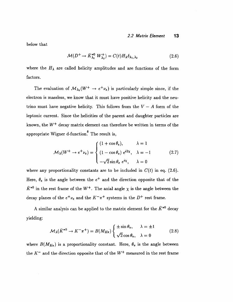
Figure 4.1 Illustration of where the different helicity rates are dominant in cosOe . cosOv space .
zero recoil momentum so that helicities are ill-defined and whence all three
must be equal in magnitude.
The top insert of Fig. 4.2 shows the derivative of the helicity rates with
respect to the form factor ratios . The longitudinal rate is a function only of Rz
whereas the transverse rates are functions only of Rv. This graph indicates
that the total rate near t = 0 is a strong function of Rz and that an excess of
events at this point would yield a lower value for Rz. The transverse terms are
not so well separated in t; most of the information on the relative magnitudes
of these rates-and therefore on Rv-comes from the cos Be dependence.
The above analysis yields a qualitative description of information on the
helicity rates available within the three-dimensional decay distribution. This
translates into information about the form factor ratios since the helicity rates

7
6
5
4
3
2
1
0
4.3 Information on Form Factor Ratios 37
- aro10Ri o 1 ... --•••~ m ar_1aF\ • ar+1aF\ • 4
0.0 0.4 t
0.8
[fil +
0.0 0.2 0.4 0.6 0.8
Figure 4.2 Helicity rates as a function oft for R2 = 0.7 and Rv = 2.0. Top insert shows the derivative of the helicity rates with respect to R2 and
Rv as a function of t.
are functions of them. Nevertheless, it would be useful to be able to quantita-
tively analyze the information available on the form factor ratios themselves.
Then it would be possible to estimate the expected errors on our measurement
of R2 and Rv as well as how much information is gained by including x in the
fit.
4.3 Information on Form Factor Ratios
The Cramer-rao theorem relates the minimum variance of an estimate
of a parameter to the information content of this parameter contained in its
probability distribution.1° For a parameter, µ, with (normalized) probability
----------- --- -

38 Information and Minimum Variance
distribution, P(x; µ),over the observable variable, x, the information per event
is:
J (ap) 2 1
I(µ)= Bµ p dx. (4.3)
The Cramer-rao theorem states that the minimum variance on an estimate of
µis given by
1 Vmin(µ) = nl(µ) (4.4)
where n is the number of events used in the estimate. If there is more than
one parameter to be estimated then the information becomes a matrix with
elements,
f (8P8P) 1 Iij(µ) = Bµi Bµj p dx (4.5)
and the minimum variance matrix is equal to the inverse of the information
matrix divided by the number of events. Note that diagonal elements of the
variance matrix may be much larger than the inverse of the diagonal elements
of the information matrix if there are large off-diagonal elements.
One can identify the locations of the minimum or maximum information
of a parameter simply by looking at a plot of the information distribution,
(8I' /8µ) 2 /r, over the observable variables. Figure 4.3 shows this forµ replaced
by R2 and Rv, over the 2-dimensional spaces in cos Bv,cos Be and t,cos Bv.
For this calculation, the total differential distribution was integrated over all
other variables except the two to be used in the plot, before calculating the
information distribution. The maximum information on R2 occurs at t = 0,
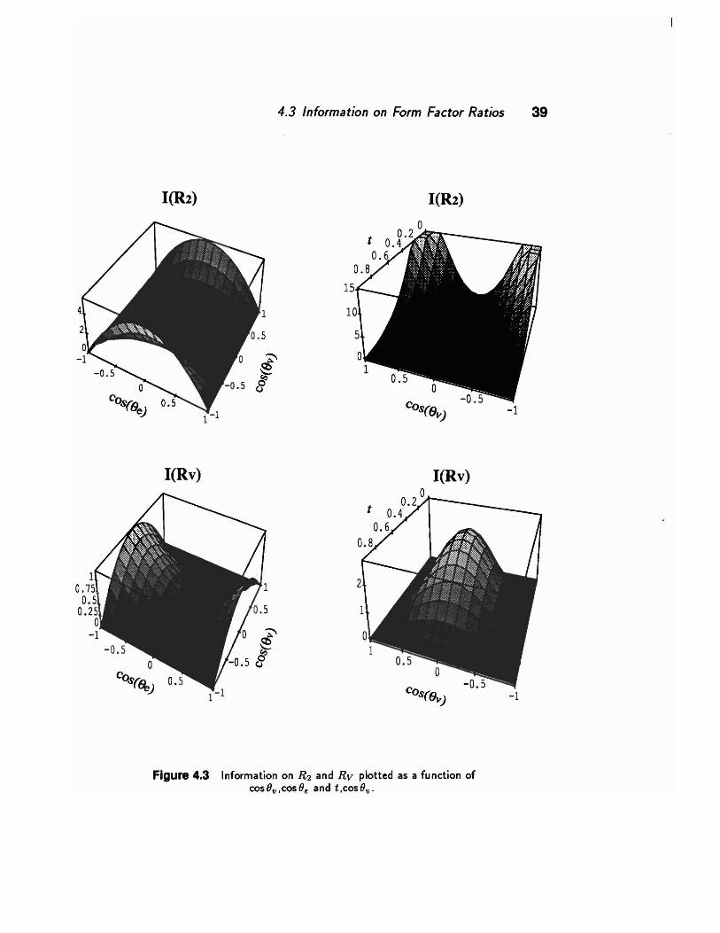
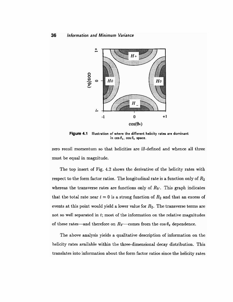
4.3 Information on Form Factor Ratios 39
l(R2) l(R2)
0 t 0 .2 ~i------0 .4
l(Rv)
0.6 0.8
15
l(Rv)
Figure 4.3 Information on R 2 and Rv plotted as a function of cosOv,cosOe and t ,cosOv .
-1
-1

40 Information and Minimum Variance
Table 4.1 Minimum errors on R2 and Rv.
Space Variables -Jn <1min(R2) Vn <Tmin(Rv) p
t, COS Ov, COS Be, X 3.53 4.64 -.30
t, COS Bv, cos Be 3.66 6.10 -.32
cos (} v , cos Be 5.70 7.10 -.49
cos Be = O, and cos Bv = ±1. There is little information about R2 at large t
and cos Ov near zero. The compliment is true for Rv except near t = tmax
where there is no information on either parameter. In addition, it can be seen
that overall there is more information on R2 due to the large peaks near t = 0.
The information matrix has been calculated for R2 and Rv for different
combinations of observable variables in two through four dimensions. Table 4.1
presents the results in terms of the minimum sigma, <Tmin(i) = Jlii, and the
correlation coefficient, p = \!i,j / JVi,i V;,;. Adding t to the fit significantly
decreases the error on R2 corresponding to a doubling of the information. The
error on Rv is also decreased but not by as much. Adding x to the fit does
not affect the precision of R2 but does decrease the error on Rv by about
25%. These calculations have not taken into account the affects of smearing
acceptance or background. The minimum errors would rise with these effects
included, with the error on R2 rising strongly if the acceptance is low near
t = 0 where the majority of the information on R2 is obtained.

5 Fit Technique
A common technique for determining physical parameters from a data set is the
maximum likelihood method in which one finds the values of the parameters
which maximize the likelihood of the data set. The likelihood is calculated from
an analytical probability distribution parametrized by the physical variables
to be estimated. Thus one might expect that to estimate the form factor ratios
all that needs to be done is to maximize the likelihood of the data using the
full differential decay rate formula, eq. (2.22). The effects of acceptance and
smearing, however, distort the data from the underlying physical distribution.
If these effects are large then an analytical form for the distorted distribution
must be found in order to perform a maximum likelihood fit. It may be very
difficult to obtain an analytical form for the distorted distribution, however,
especially over many dimensions. This is the situation we are confronted with.
We wish to make a multi-dimensional maximum likelihood fit in order to use
as much of the available information as possible; however, smearing due to
incomplete information about the neutrino is significant and very difficult to
parametrize over the multi-dimensional space of observables. This chapter first
- 41 -

42 Fit Technique
details the acceptance and smearing problem and then explains our solution
for making a maximum likelihood fit over many dimensions in the presence of
such effects.
5.1 Smearing and Acceptance
5.1.1 Smearing
As described in section 3.4 the quadratic ambiguity in the longitudinal
momentum of the neutrino causes smearing so that the calculated values of
the kinematic variables (i.e. cos Ov, cos Oe, t, and x) are sometimes different
from their true values. Another cause of smearing is limited resolution in the
direction of the D. This is taken to be the direction between the reconstructed
production and decay vertices. However, the resolution on each of these ver
tices is limited, thereby limiting the resolution on the direction of the D.
One way to see the magnitude of the smearing is to take the Monte Carlo
events and to calculate the variance of the smeared values around the true
values. This was done as a function of the true variables so that one could see
how the smearing changes over the full range of values. The results are shown
in Fig. 5.1 for all four variables. The smearing corresponds to a standard
deviation of between 10% to 30% of each variables range. Furthermore, the
largest smearing occurs near t = 0 and cos Oe = -1 which, as discussed in the
previous chapter, is where most of the information on R2 and Rv, respectively,
is contained. This means that the information contained in the data is much
less than that calculated in Chapter 4; thus, the errors on R2 and Rv will be

0.12
0.10
1I1
~ 0.08 c: ns
11 I -~ 0.06
I f H111f IH1 >
Q)
0.04
0.02
0.00
0.30
0.25
g 0.20 ns -~ 0.15 >
0.10
0.05
0.0 0.2 0.4 0.6 0.8 1.0 ti \nu
0. 00 ....._ _ _...._ _ ___,,, ____ _..
-1.0 -0.5 0.0 0.5 1.0 cos ae
5.1 Smearing and Acceptance 43
0.14
0.12
IIll111IIl1IIIIJl1 Q) 0.1 0 0
; 0.08 "ii:: ns > 0.06
0.04
0.02
0.00 -1. 0 -0.5 0.0 0.5 1.0
cos av
2.5
2.0
0.5
0. 0 ......_ ______ ___._ _____ .....
-2 0 l
2
Figure 5.1 Variance of smeared t/tmax. cosOv. cosOe. and x about the true values as a function of the true values.

44 Fit Technique
larger than the minimum errors calculated from the Cramer-Rao theorem.
The effect of the smearing on the shape of the differential decay distribu
tion is to flatten it out so that any peaks or valleys are less prominent. In
addition, the large smearing at the edge of the range of t and cos fJ e skews
the decay distribution towards higher t and cos Oe. Both these effects are
significant and need to be included in measuring the form factor ratios.
5.1.2 Acceptance
The major effect of the acceptance is due to the requirement that the
electron laboratory energy be greater than 12 Ge V which causes a low efficiency
for decays with low t and cos Oe near -1. Again the Monte Carlo events are
very useful for demonstrating this. Having generated the Monte Carlo with
a known distribution over the kinematic variables, the resulting shape of the
accepted Monte Carlo events can be compared and a shape for the acceptance
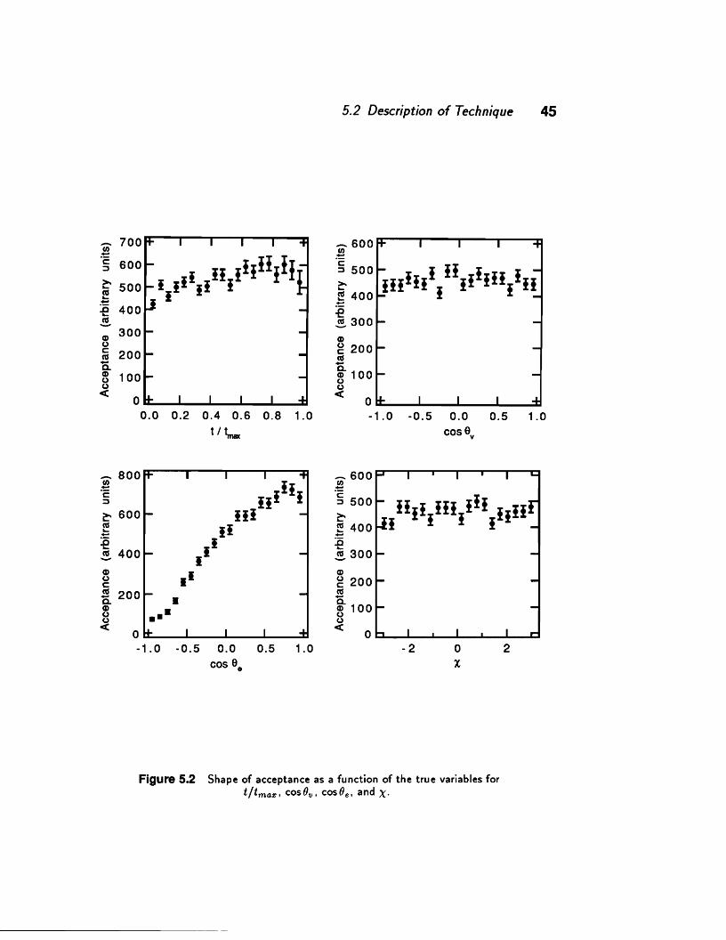
calculated. The shape of the acceptance for all four variables is shown in
Fig. 5.2. The acceptance drops about 90% from cos Oe = 1 to cos Oe = -1.
This also tends to bias the observed decay distribution towards high cos Oe thus
hiding the dominant H_ term which populates the area near cos Oe = -1.
The effects of smearing and acceptance are significant and need to be
included in the measurement of the form factors. We can use the Monte Carlo
to estimate the shape of the smearing and acceptance functions, however, it
is very difficult to parametrize them over the full four-dimensional space. For
this reason a new fitting technique was developed which is described in the
next section.
700 ~
1 H 1l1H1fl c: 600 ;:,
>. I 11 11 I 500 ... "' ... -:.0 400 ... ~
Q) 300 (,) c: 200 "' c.. Q) 100 (,) (,)
< 0 0.0
- 800 ~ ·c: ;:,
~ 600
"' !:: :e .!!. 400
I
0.2
g •• li 200 • Q)
8 •••
0.4 0.6 0.8 1.0 t It,,_
< 0-----------1.0 -0.5 0.0 0.5 1.0
cos 98
5.2 Description of Technique 45
-600 -~ c:
111l11f lll11l1111l11 ;:, 500 >. ... ~ 400 :.0 ~ 300 Q)
g 200
"' g. 100 (,) (,)
< 0 -1.0 -0.5 0.0 0.5 1.0
-600 ~
"§ 500
~
~ 400 :.0 ~ 300 Q)
g 200
"' g. 100 (,) (,)
cos9v
< 0 .._ ________ _
-2 0 x
2
Figure 5.2 Shape of acceptance as a function of the true variables for t/tmax• cos011 , cosOe, and X·
46 Fit Technique
5.2 Descrip'tion of Technique
Consider the maximum likelihood estimate of the polarization of a particle
with differential decay distribution given by f(x, µ) = (1 + µx 2). Here xis the
cosine of the decay angle and the parameter µ, which is to be estimated with
a maximum likelihood fit, is related to the polarization. The data consists of
a set of n events with values of x, {Xi}. The log-likelihood of these events is
given by n
ln L = L (in r( Xi' µ) - In N (µ)) (5.1) i=l
where N(µ) is the normalization, N(µ) = J f(x, µ) dx. The maximum like-
lihood estimate of the parameter µ is that value of µ which maximizes the
log-likelihood of the data. This is the standard maximum likelihood method
of estimation of a parameter given an analytical formula for the probability
distribution, r( x, µ ).
In our case, f ( x, µ) is the full differential decay distribution given in
eq. (2.22); x represents the variables cos Bv, cos Be, t, and x; and µ repre
sents R2 and Rv. In addition, the effects of acceptance and smearing distort
the data so that it is no longer distributed according to r(x, µ) but rather
according to some other distribution. This modified, observable distribution,
F(x, µ), which is a function of the smeared, measured variables, x, is related
to the underlying physical distribution by the equation:
F(X,µ) = A(X) j S(X,x)f(x,µ)dx (5.2)

5.2 Description of Technique 47
where A(x) is the acceptance function, and S(x, x) represents the smearing.
It is this function, F( x, µ ), which should be used in the calculation of the
likelihood, n
lnL = L(lnF(xi,µ)- lnN(µ)) i=l .
(5.3)
with N(µ) = J F(x, µ) dx. However, in order to get an analytical form for
F( x, µ ), one must have an analytical form for the acceptance and smearing
functions. Often this is accomplished by using a Monte Carlo simulation of
the experiment. This scheme becomes very difficult, however, when the space
of observables is multi-dimensional. Information about the shape of the ac-
ceptance and smearing functions is still contained in the Monte Carlo events;
it is just difficult to parametrize.
Our method uses Monte Carlo events directly in the log-likelihood cal
culation. If our Monte Carlo simulation of the experiment properly includes
the effects of smearing and acceptance, then Monte Carlo events that at the
generated level are generated according to the distribution r(x, µ),will at the
observable level be distributed according to F( x, µ ). With a large enough set
of Monte Carlo events the shape of F(x, µ) can be determined well enough so
that the log-likelihood of the data can be calculated for a given value of µ.
In order to perform a maximum likelihood fit using Monte Carlo events di
rectly there are two main problems that must be solved: (1) generating large
amounts of Monte Carlo events for different values of µ efficiently, and (2)
calculating the log-likelihood from the Monte Carlo events even though there
is not an analytical form for F( x, µ ).

48 Fit Technique
The first problem can be solved by using the same set of Monte Carlo
events and weighting each event for a given value ofµ. First, generate a set of
m Monte Carlo events which at the generator level are distributed uniformly
over the space of unsmeared observables, x. Let Yi (we use the letter y to
distinguish Monte Carlo events from data events) be the generator-level values
of the unsmeared observables for the j'th Monte Carlo event, and Yi be the
values of the smeared observables, x, for that same Monte Carlo event. Record
the set {y;, Yi} for each Monte Carlo event. Then by weighting each Monte
Carlo event with the value of r(y;, µ) using the unsmeared values, the set
{y;} of smeared values will be distributed according to F(x, µ). In this way
the same set of Monte Carlo events can be used to represent F(x, µ) for any
value ofµ.
Generating the Monte Carlo events distributed uniformly might be ineffi
cient. More generally, one can factorize the function, r(x, µ), into two terms:
one which depends on µ, W(x, µ), and one which is independent ofµ, P(x).
Then one generates Monte Carlo events according to P( x) and weights them
with W(x,µ). We chose P(x) to be the phase space distribution, including
the Breit-Wigner term, and W(x, µ)the matrix element squared.
The solution to the second problem comes from the fact that a histogram
of weighted Monte Carlo events will asymptotically become indistinguishable
from a plot of F( x, µ) as the number of Monte Carlo events increases and the
size of the histogram bins decreases. One can estimate F(xi, µ) for each data
event by forming a small volume in x space centered about Xi, summing the
5.2 Description of Technique 49
weights of the Monte Carlo events whose smeared observable values, Yi, lie in
this volume, and dividing by the size of the volume. By centering the volume
around the point of interest a linear change in F over the volume does not
contribute any error to the estimate of F( Xi, µ); only non-linear variations of F
over the volume contributes to this systematic error. In addition, each Monte
Carlo event may be in more than one volume. Normalization is accomplished
by demanding that the sum of the weights of all Monte Carlo events is unity
for each value of µ.
With this technique the log-likelihood of the set of data events is given by
lnL = tin(L:ii;inVi W(y;,µ)) i=l C(µ)Vi
(5.4)
where Vi is the volume centered around Xi and C(µ) = L:j=1 W(y;, µ) is the
normalization.
There is also some amount of background present in the data set. Having
estimated that out of a total of n events there are NB background events dis-
tributed according to a normalized distribution, PB(x), then the log-likelihood
is given by
Using this method for calculating the log-likelihood one can make a maxi
mum likelihood fit to the data over any number of dimensions even with large
smearing and acceptance effects.

50 Fit Technique
The systematic errors associated with this fitting technique are due to:
a) any non-linearity in F over the small volumes, Vi and b) limited Monte
Carlo statistics in each volume. To minimize the former, volume size should
be chosen small enough that F varies only linearly over the volume. However,
with smaller volumes, fewer Monte Carlo events will be included in the calcu
lation of F(xi, µ), which will result in an increase of the systematic error of
the second type.
One can estimate the magnitude of the first type of systematic error by
redoing the fit with different volume sizes. For very small volumes the resulting
values of µ will vary greatly due to limited Monte Carlo statistics but will be
centered around the true µ. As the volume size is increased, the variation in
the resulting values ofµ for different fits will decrease but the average should
remain centered around the true value if non-linear effects are not large at this
volume size. But as the volume size increases to where non-linear effects are
important, then the resulting values ofµ will start to diverge from the true
value. If there are enough Monte Carlo events there will be a range of volume
sizes where the resulting values of µ are fairly stable. The standard deviation
of these values within this nearly stable region is an estimate of the systematic
error of the first type.
By holding the volumes fixed and redoing the fit a number of times with
independent sets of Monte Carlo events, one can estimate the magnitude of
the systematic error of the second type. A simple way of doing this is to divide
the full Monte Carlo sample into 4 separate files and to perform the fit with

5.2 Description of Technique 51
these 4 samples. The standard deviation of the resulting values ofµ divided
by 2 is then an estimate of the systematic error of the second type, assuming
that this varies as the square root of the number of Monte Carlo events used.
If the magnitude of these systematic errors is found to be unacceptably large
then one can always reduce them by generating more Monte Carlo events.

6 Fit Results
Historically, we first measured the form factor ratios using only cos Bv and
cos Be. After being satisfied that things were working well in two-dimensions,
the fit was extended to include first t and then X· For this dissertation, the
fit will be described in detail for just the three-dimensional case and for the
addition of x since it was treated in a special way. Nevertheless, results from
the two- through four-dimensional cases are shown. Having determined the
form factor ratios, the branching ratio is measured using the measured values
of the form factor ratios to estimate the acceptance. Then using the branching
ratio value, the absolute value of Ai(O) is calculated followed by that of A2(0)
and V(O).
6.1 Three-Dimensional Fit
Monte Carlo events were generated distributed according to phase space
plus the Breit-Wigner of the .i<*0 ,
- 52 -
6.1 Three-Dimensional Fit 53
where K is the momentum of the K*0 in the rest frame of then+. To get the
distorted, observed distribution, F(i, cos Bv, cos Be; R2, Rv ), the Monte Carlo
events are weighted with the matrix element squared (after integrating over x),
W(t, cos Ov, cos O.; R2, Rv) = t{ 4 sin2 o. cos2 OvlHo(t)12
+ [(1 +cos o.)2 IH+(t)l2+(1 - cos o.)21H-(t)l2] sin2 Ov}
(6.2)
using the generated, unsmeared values of the dynamical variables. The helicity
amplitudes are parametrized by two form factor ratios ( R2 , Rv) which are the
quantities to be estimated (theµ parameters of the previous Chpt.);
Here MA= 2.53 GeV and Mv = 2.11 GeV are the values of the poles used in
assuming a single pole dominance for the t-dependence of the form factors. A
total of 9000 accepted (out of one million generated) Monte Carlo events are
used.
In calculating the log-likelihood, Monte Carlo events are binned into small
three-dimensional volumes centered about each data point. As can be seen by
the plots of the data in Fig. 6.1 at the end of this section, the distributions are
54 Fit Results
fairly linear so that bins of the order of 1/10 the range of each variable per side
should be mostly free of non-linear effects which can increase the systematic
error of the fit. This then will be a good starting volume size although different
volume sizes will need to be used in order to establish the stability of the fit
and to estimate systematic errors. We use the same volume size throughout
the three-dimensional space with the exception of data events which occur
near the boundary. For these events we shrink the volume so that the data
event remains in the center. In addition we omit from the fit any data events
whose Monte Carlo volumes did not contain at least 4 Monte Carlo events.
This only occurs near the boundaries where volumes have been decreased a
great deal and does not significantly affect the results.
The code which performs the fit consists of an initialization and a mini
mization section. The initialization section reads in the data and Monte Carlo
events, calculates the volume dimensions for each data point, and identifies the
Monte Carlo events which fall into each data event volume. Data events which
do not contain at least 4 Monte Carlo events in their volumes are eliminated
here. The minimization section consists of varying the values of R2 and Rv
until the negative log-likelihood, calculated using equation (5.5), is minimized.
In order to minimize the amount of background, the fit is performed us
ing data events which are within the K*0 mass range of (0.8408, 0.9434] GeV.
Only those Monte Carlo events whose true value of Mx1r is within this range are
also used. This is important since the value of Mx1r is used in calculating the
weights. In addition, since the maximum oft depends on the value of Mx?r we

6.1 Three-Dimensional Fit 55 Table 6.1 Results of fits for different volume dimensions.
Volume (xl0-3 ) ~cos Bv ~cos Be ~t R2 lnRv
0.004 0.033 0.027 0.05 -0.1±0.5 -0.7 ± 0.7
0.36 0.067 0.053 0.1 0.2 ± 0.5 0.6 ± 0.4
0.81 0.09 0.09 0.1 0.1±0.5 0.6 ± 0.4
1.2 0.1 0.08 0.15 0.0 ± 0.5 0.6 ± 0.4
4.0 0.2 0.1 0.2 -0.2 ± 0.5 0.7 ± 0.4
4.05 0.15 0.12 0.225 -0.l ± 0.4 0.6 ± 0.4
32.4 0.3 0.24 0.45 -0.4 ± 0.5 0.8 ± 0.4
employ the normalized variable, y = t/tmax, when comparing smeared data to
smeared Monte Carlo events in the fit. From our estimate of the total amount
of background over the full MK7r range given in Chapter 2, and the assumed
shape of the background distribution, we estimate that there are 21±5 back
ground events within the narrow M K7r range. For the background shape over
the three-dimensional space of the fit, we want to use a parametrization which
is consistent with that of the wrong-sign data. There are not many events
in the wrong-sign sample so this information is very limited. Nevertheless, it
appeared that a distribution that is uniform in cos Bv and cos Be and linear in
twas appropriate. We fit they-distribution of the wrong-sign data to a linear
function and used this, normalized over the full three-dimensional space, as
the background shape. The result is P(y, cos Bv, cos Be) = (3y + 0.2)/3.4 for
the background function.
With this method it is important to perform the fit a number of times,
varying the volume dimensions and number of Monte Carlo events used, in

56 Fit Results
Table 6.2 Result of fits with 4 independent Monte Carlo samples.
R2 lnRv
0.1 ± 0.5 0.5 ± 0.4
0.0 ± 0.5 0.4 ± 0.5
0.4 ± 0.4 0.6 ± 0.4
0.1 ± 0.4 0.5 ± 0.4
order to insure the fit is stable and to estimate the magnitude of systematic
errors. Table 6.1 shows the results of fits for different volume sizes using the
same number of Monte Carlo events. Here we have expressed the results in
terms of lnRv which has a distribution that is more nearly Normal. The errors
shown in the table are the statistical errors obtained by locating where the log
likelihood decreases by 0.5 from its maximal value. The results are fairly stable
over a wide range of volumes with the exception of the very largest and the
very smallest volumes. Neglecting these extreme cases, the average of the
remaining values becomes our best estimate of the central values. Thus our
measurement is R2 = 0.0 ± 0.5, InRv = 0.6 ± 0.4 where the errors shown are
only the statistical errors from the data.
To estimate the systematic error of the first type, we take the standard
deviation of the fit values from the trials within the nearly stable region. This
yields u1 = 0.16 and u1 = 0.04 for R2 and lnRv respectively.
To estimate the systematic error of the second type, we hold the volume
dimensions fixed at the ones shown in the forth row of Table 6.1 which yield
the best central values, divide the Monte Carlo events into 4 files, and redo

6.1 Three-Dimensional Fit 57
the fit with these 4 independent sets. The results are shown in Table 6.2. The
standard deviation of the values for R2 and lnRv is taken as an estimate of
the second type of systematic error for a quarter of the Monte Carlo events.
Assuming this error goes as 1 / VN, the error for the full Monte Carlo sample
should be half these values. This yields u2 = 0.09 and u2 = 0.08 for R2
and lnRv respectively. The total systematic error we take to be the sum
(in quadrature) of these two types of systematic errors. Thus our result is
R2 = 0.0 ± 0.5 ± 0.2, lnRv = 0.6 ± 0.4 ± 0.1, or Rv = 1.8 ± 0.7 ± 0.2,
where the first error is statistical associated with the data and the second is
systematic associated with the fit method. There is also the systematic errors
associated with the data and with the uncertainty in the background; these
will be discussed for the final four-dimensional fit in the next section.
We looked at many plots to check the integrity of the fit. Figure 6.1
compares the data and Monte Carlo distributions over various slices through
the three-dimensional space. In all cases the data and Monte Carlo follow
each other quite well. Also, one can see that the deviation of the Monte Carlo
around a smooth curve is much smaller than that of the data. This indicates
that the systematic error due to the statistics of the Monte Carlo is small
compared to that of the data.

58 Fit Results
50
40 C\I ci - 30 Cf) .... z
20 w > w
10
0 -1.0
25
20
15
10
C\I 5 ci -Cf)
0 .... z w
-0.5 0.0 cos ee
25
20
15
1 0
5 ..-ci 00 0 ....
0.5 1.0
> 20 w z w Gj
15 l1cos 9vl < o.sl
15 1 0
10
5 5
0 ._ _ __. __ ....._ _ __... __ ... o ..... ____ ....__.....__..-.~ ... -1.0 -0.5 0.0 0.5 1.0 0.0 0.2 0.4 0.6 0.8 1.0
cos 0v t I tmax
Figure 6.1 Projection of the data (dots with error bars) and Monte Carlo (solid histogram) events onto cosOe. cosOv. and t/tmaz:· The Monte
Carlo events are weighted using the measured form factor ratios.
6.2 Four-Dimensional Fit 59
6.2 Four-Dimensional Fit
In addition to the longitudinal and transverse terms in the matrix element,
there are also three interference terms which depend on the angle between the
decay planes of the e- Ve and the K- 1r+, labeled x,
-2 sin2Be sin2Bv cos 2x H+H-
-4 sin Be (1 +cos Be) sin Bv cos Bv cos X H+Ho (6.4)
+4 sin Be (1 - cos Be) sin Bv cos Bv cos X H-Ho.
These terms integrate to zero and were not used in the previous three-dimen
sional fit. The H_Ho term should be largest but only over a small region of
phase space. We have plotted the data and Monte Carlo events as a function
of X in Fig. 6.2 using the values of the form factor ratios found above. One can
see the expected cos x dependence in (a); however, the small cos 2x dependence
that is expected in (b) is lost in the limited statistics of the data. The fact
that the data and Monte Carlo projections match each other fairly well over
x provides an independent check that the data and Monte Carlo agree since
nowhere was information about x used in the previous fit.
Including x in the fit is complicated by the large smearing that occurs
when x is ill-defined. This happens when the K- 1r+ or the e- Ve lie in a line
with the direction of then+. Fortunately this is where the interference terms
go to zero. Rather than bin the Monte Carlo into four-dimensional bins, which
would have decreased the number of Monte Carlo events per bin, we decided to
do the following. We bin the Monte Carlo events into three-dimensional boxes

60
0 ,... ~ ~ ...... en t-z w > w 0 w t-:::c (!) w !:
Fit Results
35
1 5 30 (b) 1 0 0 ,... 25
~ 5 C\I 20 -......
CJ) 0 t- 1 5 z
w -5 > 1 0 w
-10 5
0 -7t 0 7t -7t 0
x x Figure 6.2 Projection of the data (dots with error bars) and Monte
Carlo (solid histogram) events onto X· In (a) events are weighted with the coefficient which multiplies the cos x term in the decay rate. This brings
out the cos x dependence. (b) is a standard projection which should have a small cos 2x dependence.
7t
as before, and when adding the weights around each data event include the
interference weights but evaluated with Xdata + Xobserved - Xgenerated replacing
Xgenerated· When the smearing is small, generated and observed x are close
so one gets the weight at the x of the data. When the smearing is large then
the weights fluctuate and add up to zero. Thus by rotating the x that goes
into the weights in this way, one is effectively getting out the weight at the x
of the data event. This works because the amount of smearing in x is largely
determined solely by the values of cos Oe and cos Ov.
Putting this into the fit we find R2 = 0.0±0.5±0.15 and Rv = 2.0±0.6±0.3
where the first error is due to the statistics of the data and the second comes
from the systematics of the fitting method calculated in the way described for

6.2 Four-Dimensional Fit 61
the three-dimensional fit. In making this fit we assumed that 21 out of the
204 data events were background and were distributed in a manner consistent
with the wrong-sign data. The choice of 21 had a standard deviation of 5,
also found from the wrong-sign data. By varying 21 by 5 either way we found
the error due to this uncertainty was .1 for R2 and .04 for Rv. The choice for
possible background distributions also led to a similarly small error.
We felt the greatest error in the Monte Carlo itself was in the electron
identification efficiency. We estimated this could be off by at most 7% and
modified each Monte Carlo event weight by 1 - .07 ~ where E is the energy
(in Ge V) of the electron in the lab frame and the 12 comes from the fact that
we have a 12 GeV electron energy cutoff. We used a linear dependence since
a constant term would go out in the normalization. The resulting deviation of
R2 and Rv was less than 10% of the error due to that of the fitting method.
Adding these systematic errors in quadrature with those due to the fitting
method yields our final result:
R2 = 0.0 ± 0.5 ± 0.2 Rv = 2.0 ± 0.6 ± 0.3 (6.5)
with correlation coefficient, PR2 ,Rv = -0.23. With these values we can calcu
late the ratio of longitudinal to transverse polarization and compare it to the
value measured earlier 11 using this same data set. That measurement found
f;: = 2.4!~:~ ± 0.2 and only used the cos Ov projection of the data. The value
using the measured form factor ratios from the full four-dimensional distribu
tion of the data is f;: = 1.8!8:~ ± 0.3. This is consistent with the previous

62 Fit Results
Table 6.3 Summary of results on R2 and Rv and comparison with theoretical minimum errors.
Space Variables Fit R2 ± u(R2 ) Fit Rv ± (TkV> mm D"(R2) min tT(RJi:::)
'Rv
t, COS 011 , COS Oe, X 0.0 ± 0.5 2.0 ± 0.30 0.26 0.17
t, COS 011 , COS Oe 0.0 ± 0.5 1.8 ± 0.39 0.27 0.23
COS 011 , COS Oe 0 4+1.0 - . -1.6 3.0 ± 0.55 0.42 0.26
result, however, the errors are smaller by more than a factor of two. This gain
in precision comes about mainly from adding t to the fit. The transverse he
licity amplitudes are proportional tot and die at t = 0, while the longitudinal
helicity amplitude has no suppression at this point. Thus one obtains very
good separation.
6.2.1 Summary
It is useful to compare the results of the fits in two through four dimen-
sions and with the minimum errors calculated in Chapter 4. This is shown
in Table 6.3. The minimum errors were calculated assuming the values of
R2 = 0. 7 and Rv = 2.0. With different values for R2 and Rv the minimum
errors will change. We have attempted to account for this by tabulating the
ratio of the error to the central value for Rv. This is not useful for R2 since the
central values are close to zero. Nevertheless, it appears from Table 6.3 that
the measured errors follow the pattern of the minimum ones quite well. The
two-dimensional fit yielded rather large errors; adding t to the fit significantly
decreased the error on R2. Adding x to the fit reduced the error on Rv. In
general, there is about a factor of two difference between the measured errors

6.3 Branching Ratio 63
and the minimum possible errors. This means that the effects of smearing and
acceptance eliminated about three quarters of the possible information. This
was expected given the poor acceptance and large smearing near t = O and
cos Be = -1 which is where the information on R2 and Rv, respectively, is
greatest.
6.3 Branching Ratio
Having obtained the form factor ratios, we re-analyze the branching ratio.
The previous measurement of the branching ratio 11
used a value for I H +I/ I H _ I
derived from a model 12
and the value of f L/fr derived from the observed
cos Ov dependence. The effective form factor ratios implicit in these values
are different from those we have measured, which affects the estimate of the
efficiency used to obtain the branching ratio. The method is to first fit the data
projected onto MK7r to obtain the number of n+ ~ J{*0 e+ve events present.
Then we calculate the efficiency for this mode and divide the found number of
events by this efficiency to obtain the total number of n+ ~ K*0e+ve events
present in the full data set. Finally we compare this number to that for the
mode, n+ ~ J<-7r+7r+, and use a previously measured value of the branching
ratio for this mode to get the branching ratio of fl+~ .f{*O e+ Ve.
To fit the data projected onto the MK?r axis we need the functional form
of the signal as well as that for the background. For the signal, we again
use the Monte Carlo events directly, weighting them using the measured form
factor ratios. We do this because phase space and the matrix element alter

64 Fit Results
the shape of the signal when projected onto the MK'lr axis so that it is not just
that of the Breit-Wigner. The previous analysis of the branching ratio 11
used
a plain Breit-Wigner shape for the signal; thus the present analysis differs in
not only using a different shape for the signal, but also a different efficiency
from different form factor ratios. We also include radiative corrections to the
electron spectrum as outlined in Ref. 13 (this only has a 0. 7% effect).
-CJ') ~
160
z 40 w > w
(a)
12 N-
0 > 10 Q)
~ l.t) 8 ~
0 ci 6 -~ 4 z w > 2 w
0 ~-....... ----i ....... _...._ _ __._;:;.:.i
0.6 0.8 1.0 1.2 1.4 2
K7t Mass (GeV/c)
0.6 0.8 1.0 2
K7t Mass (GeV/c )
Figure 6.3 (a) S-wave Monte Carlo data (dots with error bars) and fitted Gamma distribution (solid curve). (b) wrong-sign data (dots with
error bars) and its fitted Gamma distribution.
1.2
The background consists of nonresonant K-11"+ signal plus true back
ground events. To estimate the shape of the nonresonant signal, we generated
Monte Carlo events in which the K-11"+ are in a relative S-wave state. That
distribution is shown in Fig. 6.3 (a) along with a fit to a Gamma distribution
of the form, xo:e-f3x. Here, x = (MK?r - Mo), a and /3, are parameters to
be determined and Mo is set to 0.63 GeV. The estimated values of a and

6.3 Branching Ratio 65
f3 are 1.2 ± 0.1 and 8. 7 ± 0.4 respectively. For the true background we use
the wrong-sign data. Its distribution is shown in Fig. 6.3 (b) along with its
Gamma distribution. Here the values of a and (3 were found to be 1.8 ± 0.8
and 14 ± 5 respectively. So there is not much difference between the shape
of the nonresonant signal and the true background. Thus we simply use one
distribution for the background; that of a gamma distribution whose param-
eters, a and {3 are consistent with those shown above. These parameters will
be varied within the errors shown above and the fit performed a number of
times in order to estimate the systematic error associated with not knowing
the exact shape of the background.
We use a binned maximum likelihood fit with the negative log-likelihood
given by:
Nbina
-ln(L) = Ns +NB - :E Ni In [NsPs(i) + NBPB(i)] (6.6) i=l
where Ni is the number of data events in the i'th bin, Ns and NB are the
number of signal and background events, respectively, to be determined, and
Ps(i) and PB(i) are the signal and background probabilities at the MK1r value
of the i'th bin. This form of the log-likelihood includes the Poisson probability
of finding the total number of events when expecting ( N s + NB) events so
that one can extract the actual values of N s and NB from the fit instead
of just their ratio. For Ps( i) we add up the weights of the Monte Carlo
events which lie in the i'th bin, divide by the bin width, and divide by the
sum of weights of all the Monte Carlo events to insure proper normalization.

66 Fit Results
N' ~ > Q)
(.!) -ll) ll) C\I C! ._ CJ) I-z w > w
80
60
40
20
• Data - Fit Function - Bckd.
0.7 0.8 0.9 1.0 1.1 1.2 1.3 2
K1t Mass (GeV/c )
Figure 6.4 Histogram of K 11'" mass distribution together with that of the fitting function. The shape of the background used in the fit is also shown.
For PB(i), we simply take the value of the normalized Gamma distribution
at the central value of MK'lr for the i'th bin. The fit is made in the MK1r
mass range, [0.6371, 1.4021] Ge V where there are 317 data events. We find
Ns = 209 ± 18 ± 9 and NB= 108 ± 17 ± 9. The systematic errors are 2.7%
from the choice of binning, 3.3% from the uncertainty of the background shape,
and 0. 7% due to the errors of R2 and Rv. The resulting signal plus background
shape together with that of the data is shown in Fig. 6.4. The previous analysis
found 227 signal events. The difference is due to the modifications of the Breit-
Wigner shape described earlier.
The efficiency is calculated by summing the weights of the accepted Monte
Carlo events and dividing by the sum of the weights of the generated Monte

6.3 Branching Ratio 67
Carlo events. Again, the measured values of the form factor ratios are used
when calculating the weight for an event. With these form factors, the ef
ficiency is found to be (1.32 ± 0.03 ± 0.09)%. Here the systematic error is
dominated by the 7% error on the electron identification efficiency. The effi
ciency corrected number of n+-+ K*0e+ve events is thus 15870 ± 1330 ± 1320
where the errors on the efficiency are treated as systematic. To correct for
a possible contamination from n+ -+ K-7r+7r+7ro a Monte Carlo simulation
of this mode was performed. The efficiency for a n+ -+ K-7r+7r+7ro event
to simulate a n+-+ k*0e+ve event was found to be 3 x 10⁻⁵ • Assuming a
branching ratio for this mode of 7%, we expect about 0.5% of the data events
to be from this mode. To correct for this we lower the efficiency corrected
number of events by 0.5% to obtain 15790 events. This number, however, only
includes k*0 -+ K-7r+. A third of the time, k*0 decays to K 07r0 • Thus the
actual efficiency corrected number of fl+-+J?*Oe+ve is 23690±1990±1970.
To obtain the branching ratio we compare to the mode n+ -+ K- 7r+ 7r+
such that
Br(D+-+ K*0e+ve) _ N(k*0) £(K-7r+7r+) Br(D+ -+ K-7r+7r+) - N(J<-7r+7r+) £(K*0 )
(6.7)
where N is the efficiency corrected number of events and £ is the effective
luminosity for each mode. It turns out that this ratio of luminosities is not
one but 1.045 ± 0.01 due to some runs being missed in the stripping process.
Then+-+ K-7r+7r+ mode has been standardized within E691 since it is used
as a normalization mode. The efficiency corrected number of n+ -+ 1<-7r+ 7r+
•

68 Fit Results
events is 51870 ± 1820. From equation (6.7) we obtain a branching ratio
for n+ ~ K*0e+ve of (0.48 ± 0.04 ± 0.04)Br(D+ ~ K-1r+1r+). Using the
measured value of Br(D+ -~ K-1r+1r+) = (9.11 ± 1.3 ± 0.4)% obtained by
the Mark III collaboration 14
and treating the errors in this measurement as
systematic, yields
+ -.o + Br(D ~ K e Ve) = ( 4.4 ± 0.4 ± 0.8)%. {6.8)
This is not much different from the 4.5 value found in the previous analysis 11
because although the efficiency went down, so did the number of observed
events.
6.4 The Normalized Form Factors
We calculate Ai (0) by equating the total decay rate of this mode to the
measured branching ratio divided by the lifetime of then+. The total decay
rate is given by
where the helicity amplitudes, given in eq. (6.3), depend on the values of R2
and Rv. We use the measured values of the form factor ratios, the branching

6.4 The Normalized Form Factors 69
ratio, and the lifetime 15
TD+ = 1.090 ± 0.030 ± 0.025 ps, all obtained from the
E691 experiment. With Vcs = 0.975 we find
Ai(O) = 0.46 ± 0.05 ± 0.05 A2(0) = 0.0 ± 0.2 ± 0.1 V(O) = 0.9 ± 0.3 ± 0.1.
The statistical error for Ai (0) comes from a statistical error of 0.04 and 0.02
for the form factor ratios and the branching ratio, respectively. The A1 (0)
systematic error is built out of systematic errors of 0.02 and 0.04 for the form
factor ratios and the branching ratio, respectively. Only the uncertainty of R2
and Rv contributes significantly to the errors of A2(0) and V(O).
The only assumption that is made in measuring the form factors is the
dependence on t. Because of the limited range oft (tmax/M; = 0.2, where Mv
is the value of the vector pole mass), the results are only sensitive to the slope
of the form factor near t = 0, and only mildly sensitive to that. In some models,
other forms for the t dependence are used, but they are effectively equivalent
at the present level of the measurement. The only quantitative information
on the t dependence of charm form factors comes in the D0 ~ I<- e+ Ve mode,
in which the pole mass is measured directly.i6
That result can be expressed as
f(t) = fp(t)(l +St), where fp is the simple pole form with the vector mass
and Sis a measure of the correction to the slope, which was measured to be
0.00±0.07. A similar uncertainty in the pole form used for the present analysis
would cause an additional error of ±0.015 in Ai (0), ±0.04 in A2(0), and ±0.02
in V(O). When these errors are added in quadrature to other systematic errors,
the total systematic error does not change at the level of precision quoted; those

70 Fit Results
systematic errors are in turn smaller than the statistical errors. Thus there
is no significant change in the form factors unless the t dependence is both
outside the range of models and in complete disagreement with that measured
in D 0 --.. K- e+ lie.

7 Conclusions
Having determined the form factor values we compare these results with those
of other experiments and predictions from theory. Finally we look to the future
and examine how these and future measurements of charm form factors will
effect the determination of the Kobayashi-Maskawa matrix elements, Vcb and
7 .1 Other Experiments
After we published the measurement of the form factors 17
two other exper-
imental groups subsequently made their own measurements: Fermilab exper
iments E65318
and E687.19
Both these experiments observe the semi-muonic
decay n+ --+ f<*O µ+ve. The same form factors govern this decay~ The only
significant effect of the muon is to increase the lower limit oft from the elec-
tron mass squared to that of the muon mass squared. This effect was included
in the measurement by E653 and they were able to demonstrate that the mea-
* A fourth form factor which is always proportional to the lepton mass in the decay rate
is still not important for muons.
- 71 -

72 Conclusions
Table 7.1 Results from this work compared with those of other experiments.
E691 E65318
E68719
Wtd. Avg.
R2 0.0 ± 0.5 ± 0.2 0.8 ± 0.2 ± 0.1 0.5 ± 0.4 0.65 ± 0.1
Rv 2.0 ± 0.6 ± 0.3 2.0 ± 0.3 ± 0.2 2.1±0.6 2.0 ± 0.3
Ai(O) 0.46 ± 0.05 ± 0.05 0.49 ± 0.07 0.475 ± 0.05
A2(0) 0.0 ± 0.2 ± 0.1 0.4 ± 0.14 0.2 ± 0.2 0.26 ± 0.1
V(O) 0.9 ± 0.3 ± 0.1 1.0 ± 0.3 1.0 ± 0.3 1.0 ± 0.2
sured form factor ratios were stable with respect to a cut on the minimum
allowed value of t / tmax.
Table 7 .1 compares the results of this work with those of other experiments.
The weighted average (as used by the Particle Data Group) of the results for
each quantity is also listed. The E687 group has only presented results on the
form factor ratios. We use the weighted average of Ai(O) to compute the values
of A2(0) and V(O) from their measured form factor ratios. Both the E653
and the E687 results are consistent with ours with the greatest discrepancy
occurring for A2(0) and R2 where there is about a two sigma difference.
Perhaps the most surprising aspect of the E653 result is that their errors for
the form factor ratios are so small; they are a factor of two smaller than ours.
Yet, they do not have much more data than we do; we have 204 events with
21 as background whereas they have 305 events with about 20 as background.
They do have better vertex resolution and acceptance, however. One can check
whether it is actually possible to obtain such small errors by using the results
presented in Chpt. 4 on the minimum possible errors. Those results, scaled for

7.2 Comparison with Theory 73
Table 7.2 Comparison of measured form factors with theoretical predictions.
Group V(O)
Experiment Wtd. Avg. 0.475 ± 0.05 0.26± 0.1 1.0 ± 0.2
Models
Sum Rules
Lattice
ISGW20
AW/GS21
BSW22
KS23
BBD24
AOS25
BKS26
0.8
0.8
0.9
LO
0.5 ± 0.15
0.9 ± 0.2
0.8
0.6
1.2
1.0
0.6 ± 0.15
0.8 ± 0.3
1.1
1.5
1.3
1.0
1.1±0.25
1.7 ± 0.6
0.8 ± 0.14 ± 0.3 0.6 ± 0.14 ± 0.2 1.4 ± 0.5 ± 0.5
LMS27
0.52 ± (0.07 x 3) 0.1 ± (0.35 x 3) 0.85 ± (0.08 x 3)
285 events are: O'min(R2) == 0.21 and O"min(Rv) = 0.28 to be compared with
E653's measured statistical errors of 0.23 and 0.33 respectively. Thus their
errors are right at the minimum possible edge. This is surprising given the
existence of acceptance and smearing effects plus background in the real data
which are not included in the calculation of the minimum possible errors.
7 .2 Comparison with Theory
To expedite comparisons, the weighted average of the measured form fac-
tors are listed together with theoretical predictions in Table 7.2. All of the
models fail to predict the low measured values of the two axial vector form
factors. This observation is even more striking when one takes into account
the fact that there is generally good agreement between predicted and mea-
sured values of the vector form factor governing the decay D ~ /{eve. Thus
74 Conclusions
it appears that the models systematically fail with axial vector form factors
but succeed with vector form factors.
After the discrepancy between the models and measured values became
known, BSW reanalyzed their model to see if this discrepancy could be rec
onciled:8 They found that the form factors had a strong dependence on the
value of a quarkmass-dependent integral over the meson wave functions. They
therefore let the value of this integral be a free parameter and listed the value
of the form factors as a function of this parameter. However, this modification
left the ratio, Rv, constant at 1.4 which is about two sigmas away from the
weighted average of the measured values, 2.0 ± 0.3. Similarly, ISGW tried to
reconcile the non-relativistic quark model but found that only a 20% change
could be affected-which is not enough~9
Unfortunately, the QCD Sum Rules and Lattice QCD results, which have
a stronger grounding in the Standard Model, are at present not known very
precisely so that they are consistent, at about the two sigma level, with both
the measured values and the model values. Nevertheless, the central values
from these two approaches tend to be going in the right direction, towards
lower values for the axial vector form factors.
The application of HQET symmetries to this decay is difficult since the
corrections are of the order AQcD /Ms which is between 70 and 200%. So
clearly, at least the first order corrections would need to be calculated in order
to even guess at the form factors from an H QET point of view. The first
order corrections have been calculated for b ~ c decay using QCD sum rules~

7.2 Comparison with Theory 75
The form factor ratios, R2 and Rv, are defined for B --+ D* lv1 decay in the
same way as for charm decay and in the limit of exact HQET symmetry these
quantities are unity. It is interesting to note that the first order corrections
for the b decay form factors find R2 decreasing by 10% and Rv increasing by
about 30%.
Although the D+-+ J{*0e+ve form factors appear to be difficult to calculate
theoretically, fortunately, they can be measured and this information is useful
in itself. For example the measured charm factors can be used to test the fac
torization hypothesis in charm hadronic decays, be related to the form factors
in B--+ K*e+e- using the symmetries of HQET,7
and serve as a significant
test for any future theory which attempts to calculate heavy quark semilep
tonic form factors. In addition, the method developed here for measuring form
factors from the complete di:ff erential decay distribution serves as a prototype
for similar measurements in the decays B -t D* lv1 and D ~ plvz which are
needed to determine the important Kobayashi-Maskawa matrix elements, Vcb
and Vub·

APPENDIX A
Cleo-II Silicon Detectors
Silicon vertex detectors have been successful in identifying charm meson de
cay vertices in fixed target experiments such as E691 and are now finding use
in collider experiments for tagging events with heavy quarks and measuring
lifetimes. A silicon microstrip detector is presently being constructed for the
CLEO-II experiment at the CESR e+e- collider, operating at center of mass
energies close to the i(4S). This detector will permit the identification of
detached decay vertices from charmed mesons, tau leptons, and other long
lived particles. Since the momentum spectrum of tracks at the i( 48) is soft
the detector must be as low mass as possible; in addition, it must provide z
measurements in order to reconstruct vertices in 3 dimensions. These consid
erations have led to the use of double-sided silicon microstrip detectors.
Double sided silicon detectors operate in the same manner as for the single
sided detectors described in Chpt. 3. The main difference is that instead of
having a uniform layer of n-type material on the back, there are a set of strips
of n-type material. This is shown in Fig. A.1. These strips, when biased,
attract the cloud of electrons that are generated by an ionizing particle, so
that the position of the ionizing particle can be determined on this n-side in
the same manner as for the p-type strips on the opposite side of the detector.
By orienting then-strips perpendicular to those on the p-side, both the x and
y positions of the ionizing particle can be measured. There is an additional
feature that makes the n-side a bit more complicated than the p-side. An
- 76-

Comparison with Theory n
n-side It' readout strips ~
Bulk Silicon
p-side readout strips
Figure A.1 Schematic of a double sided silicon detector.
accumulation layer of negative charge carriers exists at the interface of the
Si02 and the bulk silicon which is highly conductive. This would serve to short
all the strips on then-side. To isolate then-strips, p-type strips are deposited
between the n-strips which drive away the electrons in the accumulation layer.
This is also shown in Fig. A.1.
Instead of using a fan-out printed circuit board to connect the sense strips
to the (rather large) preamplifiers as was done in E691, here the preamplifiers
for a whole set of strips (64 to be exact) are formed together into one chip which
can be bonded directly to the silicon detector. The CAMEX multiplexing
amplifier, developed at the MPI-Munich 30
is used as the preamplifier for both
the n- and p-strips. The rest of this appendix describes the results of studies
done by the author for high signal/noise operation of the silicon microstrip
detectors using the CAMEX.

78 Cleo-I I Silicon Detectors
R1 R2
~ Input ~ Output
r U1 ~ CSA1
~ Test Pulse CSA2
Line
Figure A.2 Schematic of a single channel of the CAM EX.
A.1 Operation and Gain of the CAMEX
A schematic diagram of a single channel of the CAMEX is shown in
Fig. A.2. The principle of operation is to sample the charge present on the
sense strip four times before and after the passage of an ionizing particle and
to take the difference. The series of events which allows this to happen is
given here. Once RI is opened, charge at the input is converted into voltage
at Ul. The switches, Sl through S4, are sequentially closed and reopened. If
R2 is closed, the closing of each S switch will bring charge into the right side
of the four capacitors to keep the voltage zero on that side. Then when R2 is
opened, the closing of each S switch will put charge on the capacitor across
the second amplifier equal to the amount of new charge that is needed at each
sampling capacitor. The net result is that the output voltage, at the closing
of each S switch, will be proportional to the charge difference at the input
between when that S switch was closed (before R2 was opened) and when
that S switch was closed (after R2 was opened). The output of each sampling
capacitor is summed to produce the final output. So ideally this results in
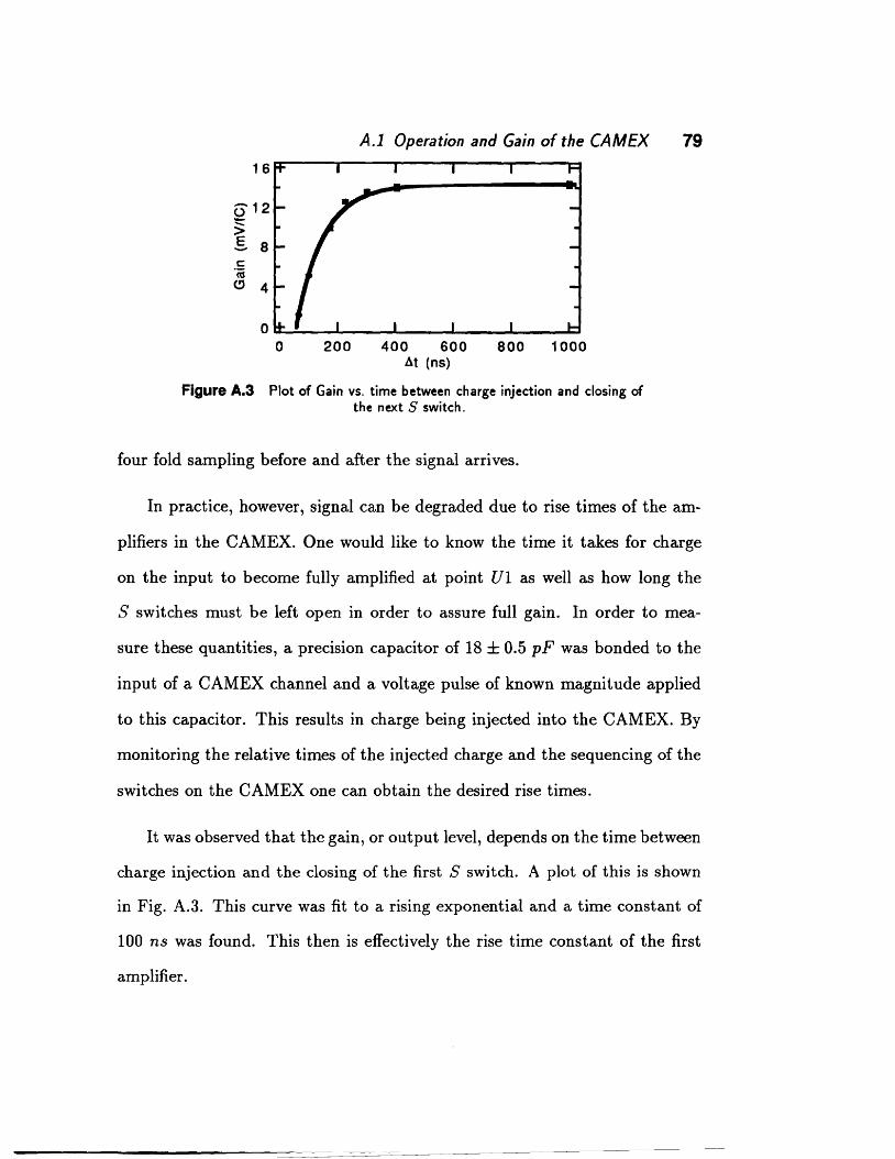
A.1 Operation and Gain of the CAM EX 79
0 200 400 600 800 1000 At (ns)
Figure A.3 Plot of Gain vs. time between charge injection and closing of the next S switch.
four fold sampling before and after the signal arrives.
In practice, however, signal can be degraded due to rise times of the am-
plifiers in the CAMEX. One would like to know the time it takes for charge
on the input to become fully amplified at point Ul as well as how long the
S switches must be left open in order to assure full gain. In order to mea-
sure these quantities, a precision capacitor of 18 ± 0.5 pF was bonded to the
input of a CAMEX channel and a voltage pulse of known magnitude applied
to this capacitor. This results in charge being injected into the CAMEX. By
monitoring the relative times of the injected charge and the sequencing of the
switches on the CAMEX one can obtain the desired rise times.
It was observed that the gain, or output level, depends on the time between
charge injection and the closing of the first S switch. A plot of this is shown
in Fig. A.3. This curve was fit to a rising exponential and a time constant of
100 ns was found. This then is effectively the rise time constant of the first
amplifier.

80 Cleo-I/ Silicon Detectors
16 • • • •
212 • - • > E -s c:
"iij C) 4
0 0 50 100 150 200
l1t (ns)
Figure A.4 Gain vs. width of S switch.
Since the values of the capacitance and applied voltage were measured,
one can obtain the absolute gain of the CAMEX by the relation Vou.t = GCVin
where G is the Gain. From the value of Vout when the output has risen to its
maximum value one obtains a gain of G = 14.3±0.3 mV/ JC for a total of four
samples. For this paper, a Gain of 14 mV/ JC will be assumed throughout
unless explicitly stated otherwise.
It was also observed that the output level decreases if the time that the
S switch is open decreases below a certain value. With the same setup as
described above, the width of the S switch was varied, making sure that the
switch did not open till at least 500 ns after charge was injected. The resulting
plot of effective gain vs. switch open time is shown in Fig. A.4. The switches
must be open for no less than 100 ns in order to achieve full gain.

A.2 Noise Studies 81
A.2 Noise Studies
In general, operation of the CAMEX requires considerable care in order to
minimize noise. Adding a detector only compounds the problem. This section
presents the results of some studies which sought to identify sources of noise
and what can be done to reduce or eliminate their effects.
A.2.1 CAM EX Without Detector
Much can be learned by studying the dependence of noise on the time
between S switches. We define the sampling time of the CAMEX, T8 , as the
time between the falling edge of successive S switches. For a CAMEX without
a detector connected, the noise has been found to be independent of this sam-
pling time. The best noise value observed, using all the known noise-reducing
techniques listed below, is an equivalent noise charge (ENC) of 290 e- ~ In
addition to the incoherent noise stated above there is a coherent noise (com-
mon to all channels on the CAMEX) that has been subtracted in software.
This noise is usually between 100 and 200 e- (added in quadrature), again
using all known noise-reducing techniques. Furthermore, both the coherent
and incoherent noise are fairly uniform across all channels. Fig. A.5 (a and
b) shows the total noise for each channel and the noise after subtracting the
common mode component.
The most drastic of the techniques used for reducing noise is the grounding
of test pulse lines at the hybrid. As shown in Fig. A.5 (a' and b') the noise
* ENC is defined as that charge, Q, on the input of the CAMEX which would result in a signal whose magnitude is numerically the same as that of the u of the noise.

82 Cleo-II Silicon Detectors
12000
80
•) ~)
8000
c -~ Q Q
~ 40 ~ -.. "-. b 4000
0 0
'° b) b)
2000 -- t> .. t> 40 Q q ~ "'C ,; -.. -. tOOO
20
0 _________ ........___.... ___ _,
0 . 32 64 32
Channel Number Channel Number
Figure A.5 Total noise (a) and noise after subtracting the common mode component (b) vs. channel number. This is with all known
noise-reducing techniques being used. Total noise (a') and noise after subtracting the common mode component (b') vs. channel number. This is
from a CAMEX without the testpulse lines grounded.

A.2 Noise Studies 83
without the testpulse lines grounded is very large and there is a distinct pattern
for every third channel. This pattern, in fact, was a clue that the testpulse lines
were involved since the three testpulse lines connect every third channel and
one of the testpulse lines starts at the high channel number end. The other two
testpulse lines start at the low channel number end. It was discovered that
charge injection effects from the S switches opening and closing were much
larger than on the CAMEXes from an older batch which did not show this
noise pattern. It is believed that these charge injection effects which appear
as variations on the output line were being picked up by the testpulse lines
along the strip cable which contains them both. The testpulse lines connect
to capacitors which inject charge into the input of the CAMEX. The testpulse
capacitors have been measured to be 0.63 pF so that noise on the order of
a thousand electrons could result from voltage variations of only a millivolt.
This problem was compounded by the fact that the output line driver on the
hybrid was amplifying signals with frequencies of 1 MHz and above and the
charge injection occurred at the sampling frequency which was 2.5 MHz. This
latter problem was easily eliminated by shorting out the line driver, but the
bulk of the noise still remained. Various grounding and shielding techniques
were tried but the only way that was found that could eliminate the problem
was to ground the testpulse lines at the hybrid.
The problem with grounding the testpulse lines is that one can not use
them for testing gains on the CAMEX. In order to try to preserve the ability to
test gains on the CAMEX a voltage divider was added to the testpulse lines at

84 Cleo-I/ Silicon Detectors
the hybrid, with all three testpulse lines connected together. It was found that
a factor of 100 in attenuation was sufficient to suppress the charge injection
effects to an acceptable level. With this attenuation, an ENC of 340 e- was
obtained but with a large common mode noise of 1000 e-. The large common
mode noise appears the same as when the testpulse line pads on the CAMEX
are left unbonded and therefore ungrounded. So it appears that the resistor
used in the voltage divider (resistors as low as 10 n have been tried) leave
the testpulse lines effectively ungrounded. At this point in time the effects
of attenuating each test pulse line separately have not been investigated, nor
have the effects of using a solid state switch.
In addition to noise resulting from pickup on the testpulse lines, a num
ber of other sources have been identified and are listed together with their
magnitude and remedy below:
1. The average pedestal level, or nominal output level of a CAMEX, changes
as a function of the time between the last reset of Rl and the trigger
(opening of R2). Fig. A.6 shows the average pedestal level, in electrons,
for the 64 channels of a CAMEX plotted against the time difference be
tween the reopening of Rl and the opening of R2 (arrival of trigger).
One can see that for times up to about 160 µs the average pedestal
level is changing by many thousands of electrons. This is probably due
to charge injection effects from the reopening of Rl being propagated
through the CAMEX electronics. If one operates in such a way that
triggers arrive at various time intervals after resetting Rl, and with at

A.2 Noise Studies
-~ 6000 'S • g. 4000 ::I 0 a; 2000 I c: c: ns 0 .z=. • (.)
I I &-2000 J e ~-4000 < 0 100 200 300
at (µs)
Figure A.6 Average pedestal level vs. time between opening of Rl and opening of R2.
85
least some triggers arriving within 160 µs, then the resulting variations
in pedestals will appear as common mode noise. The magnitude of this
noise could be as large as thousands of electrons. One could, in prin-
ciple, eliminate this noise by operating in such a way that the trigger
arrives at precisely the same interval. However, the slope of this plot
is sufficiently large that one would need to insure that the interval was
constant to a high degree of precision. The other alternative is to simply
veto all triggers until 160 µs after the reopening of Rl. It is expected
that it will be possible to run in this manner at CLEO without much
increase in dead time.
2. It has been found that noise, both coherent and incoherent, is reduced by
100 to 200 e- by shielding the cable carrying all the input and output
lines to the CAMEX, and by not connecting this shield to ground at
either end. The reason for this latter part is not understood, but for
the former it is believed that shielding reduces the effects of pickup

86 Cleo-I I Silicon Detectors
among the various input and output lines within the cable. Obviously,
the amount of pickup will depend on the particular circumstances of
any given setup, nevertheless, it will remain true that it is important to
shield and isolate both input and output lines as well as possible.
3. There can be variations between the ground of the CAMEX and the
ground of the ADC electronics. These variations will appear as noise on
the digitized output. An effective way to reduce this is to amplify the
output signal close to the CAMEX. This not only reduces the effects of
changing grounds, but also reduces the effects of any pickup the might
occur along the cable connecting the output to the ADC. For the present
setup, it was found that by amplifying the output by a factor of 10,
reduced the common mode noise by about 50 e- and the incoherent
noise by bout 100 e- (in quadrature).
A.2.2 CAMEX With Detector
With the addition of a detector noise increases due to the capacitance on
the input of the CAMEX as well as noise from the detector itself. In addition,
it has been found necessary to filter the bias line supplying the bias voltage
for the detectors with a simple RC filter. This is necessary, in that if the filter
is not present then noise, both coherent and incoherent, will be present at the
level of the expected signal size. What has been done is to connect the bias
line to the bias pad on one side of the detector through a IMO resistor and
then connect the ground from the power supply to the bias pad on the other
side of the detector, with a capacitor across the two sides of the detector. For

A.2 Noise Studies 87
the detectors and power supplies used thus far, a value of RC ~ 5 x 10⁻² s has
been found to be sufficient. It is not clear how universal this number is; one
may need a larger value depending on the particular detector or power supply
used. Furthermore, by measuring the voltage drop across the lMf! resistor,
one can monitor the leakage current of the detector.
The noise resulting from the capacitance that the detector adds to t.he
input of the CAMEX is actually due to the series voltage noise from the
first amplifier in the CAMEX. The capacitor turns this into charge noise at
the input of the CAMEX. According to the CAMEX spec. sheet, the total
noise increases roughly linearly with input capacitance with a slope of about
30 e-/pF.
With the addition of a detector, the noise is also found to increase with
increasing sampling period, Ts· This was not the case for a pure CAMEX so
this noise must be from the detector. A plot of noise squared versus Ts is
shown in Fig. A.7 for the p-side of the detectors~ The noise grows rapidly
with Ts so that at above 1 µs the detector noise dominates. But at 400 ns,
which is close to the sampling period which is expected to be used in CLEO,
this noise is minimal. Fitting this plot to a quadratic yields
where Ts is in µsand ENC is in electrons. The constant term implies an ENC
of 332±15 e-.
* The conversion between electrons and ADC units is 1 ADC= 58.3 e-.

88 Cleo-I I Silicon Detectors
600
500
-400 N(.)
c 300 ~
Nt) 200
100 o.._. __ ........ .__ __ _._ __________ ..._ __ _.. ______ _
0 2 5 6
Figure A.7 Noise squared plotted as a function of the sampling period, T,, for the p-side of a detector. The line is a fit to the data using a second
order polynomial.
For the n-side of the detectors with polysilicon bias resistors and wide p-
barriers the noise squared is shown in Fig. A.8. As can be seen, the noise is
approximately linear in this case with the parametrization being given by
ENC2( 'Ts) = (2.7 ± 0.3) x 105 + (1.26 ± 0.07) x 105
'Ts. (A.2)
The constant term is much bigger here and translates into an ENC of 520 ±
29 e-. Attempting to understand these plots in terms of the expected sources
of noise in the detector is the subject of the next section.
A.3 Noise as Information
It is important to try to understand the source of noise intrinsic to the
detector. As was seen in the previous section, this noise is different on the p-
side than on the n-side. If one could identify the source of this difference, one
might be better able to reduce the noise. The expected sources of noise are the

A.3 Noise as Information 89
300
250
-200 N(.)
0 150 ~
Nt:) 100
50
o.._ __________ .__ __ __.~ __ ...... ____ _._ ____ .-... 0 2 4 5 6
Figure A.8 Noise squared plotted as a function of the sampling period, r,, for the n-side of the detectors. The line is a fit to the data using a first
order polynomial.
thermal or Johnson noise from the bias resistor, and shot noise associated with
the leakage current. This section is devoted to the attempt at understanding
the observed noise results in terms of these sources.
A.3.1 Theory
The relationship between observed noise spectrum and noise source is given
by
00
u2 = ~ J N(w) IH(w)l2 dw (A.3)
0
where N ( w) is the spectral power density of the noise source and H ( w) is the
transfer function of the electronics connecting the point of origin of the noise
with the output~1
As an example, consider the case of a RC circuit where the
noise source is the Johnson noise of the resistor and the output is the charge
on the capacitor. The Johnson noise may be considered to be a parallel source

90 Cleo-I I Silicon Detectors
of current with a spectral power density of32
N(w) = 2kT = d(/2
) R dw
(A.4)
This noise spectrum is constant for all frequencies and is therefore also called
white noise.
I c
....,_ _____ , Q
R out
Figure A.9 Diagram of RC circuit showing thermal noise as a parallel source of current noise, I.
The equivalent circuit with current source, I, is shown in Fig. A.9. The
transfer function between the current source and the output is H(w) = l-~w°Rc·
The mean square charge noise on the output is then
(A.5)
The effect of the electronics, which takes the current source to the charge
sensitive output, is to change the frequency shape of the noise from one that
is constant to one that decreases as ~ for w ~ -Ile. In this case, the total
noise on the output is independent of R.

A.3 Noise as Information 91
For silicon detectors, a similar circuit applies. Here, the resistor is the bias
resistor and the capacitor represents the AC coupling capacitor. The charge
at the output goes to the input of the CAMEX. In addition, there is a parallel
capacitance which is dominated by the interstrip capacitance. This makes the
transfer function l-iw:{b+ci).
Shot noise from the leakage current of the detectors is also present. This
noise has a white power spectrum as well, with amplitude ql where q is the
charge of the electron, and I is the leakage current~3
The total noise power
spectrum is then the sum of the Johnson and shot noise power spectra.
A.3.2 Effect of CAMEX on Noise Spectrum
The CAMEX has its own effective transfer function which will modify the
noise spectrum and it is necessary to know this function if one is to understand
the observed noise. To obtain the total noise in an extended series of electronics
one simply multiplies the absolute square of the separate transfer functions
together and integrates this with the total noise spectral power density. With
H ( w) being the transfer function of the C AMEX, the total mean square charge
noise on the output of each channel of a CAMEX due to the Johnson and shot
noise is given by
(A.6)
The transfer function of the CAMEX may be obtained by taking the
Fourier transform of the time-dependent impulse response function of the

92 Cleo-// Silicon Detectors
CAMEX; this is the response of the CAMEX to a delta-like charge pulse.
For an ideal CAMEX, with zero rise and fall times, the quadruple sampling
produces the impulse response function
) G{ ( Ts 3Ts 5Ts 1Ts h(r =- 6r--)+6(r--)+8(r--)+8(r--)
4 2 2 2 2
( Ts) 3Ts 5Ts) ( 7Ts } -8 T + - - 6(T + -) - 6(T + - - 8 T + -) 2 2 2 2
(A.7)
where Ts is the sampling time and G is the gain for four samples, 14 mV/ JC.
Taking the absolute square of the Fourier transform of this function yields
This function, the noise weighting function of the CAMEX, is periodic and does
not decrease for large w. For high frequencies, the rise time of the CAMEX
comes into play, reducing the effects of the high frequency noise. It was shown
in the first section that the effective rise time constant of the CAMEX is 100 ns.
One may include this effect by multiplying an additional factor of 1+ 12 2 , W TR
where TR is the rise time constant, to the above noise weighting function.
A.3.3 Testing CAMEX Noise Weighting Function
It is important to be confident that this weighting function, and the pro-
cedure for obtaining the total noise, is correct. One piece of evidence is that
the weighting function for one sample, obtained in the above manner, agrees
with the one obtained in an early paper on the CAMEX. 34
Another check
is to compare the noise predicted using the above weighting function to the

A.3 Noise as Information 93
measured noise from a known source. What was done was to inject charge into
the CAMEX with a sine wave of known frequency and amplitude. A function
generator was connected to a capacitor of C = 4.7 pF which was bonded to
the input of a channel on a CAMEX. Since the input is of a single frequency,
the total noise on the output is simply given by
G A u = -IH(w)IC 10 4 v2
(A.9)
Here C ~is the power of the input noise of angular frequency, w, where A is the
amplitude of the input voltage sine wave. This is plotted in ADC units perm V
of input voltage as a function of the frequency of the sine wave in Fig. A.10.
By varying the frequency of the function generator, this same pattern was
observed on the output of the CAMEX. The maximum and minimum occurred
at the frequencies expected. Moreover, the sigma of the output was measured
for frequencies of 189 kHz and 108 kHz with amplitudes of 5 m V and 10 m V
respectively. For the former case, the observed sigma was 260 and the expected
value using the above weighting function is 265. For the latter frequency, the
observed sigma was 198 and the expected value was 200. Taking into account
the uncertainties involved (about 5% just for the capacitance) there is good
agreement between the predictions of this model and the observed results.
A.3.4 Evaluation of Total Noise Integral
Confident that the weighting function is correct, let us turn to the main
problem of calculating the expected noise from the Johnson and shot noise
sources. At this point, this amounts to performing an integration. One can

94 Cleo-// Silicon Detectors
50
40
30
20
10
0.1 0.2 0.3 0.4
Figure A.10 Calculated noise in ADC units on the output of a CAMEX with a sampling period of 5.8µs, for an input sine wave voltage of lmV
through a capacitor of 4.1pF. Th~s is plotted vs. frequency, in MHz, of the sine wave.
simplify this integral by noting that the effect of the rise time of the CAMEX
can be neglected without much error as long as the sampling time is large
compared to the rise time. In doing so the noise will be only underestimated,
with the amount of this error increasing for smaller sampling times. Also, it is
useful to rewrite the noise weighting function so that all terms are of the form,
sin2(x), using trigonometric identities. Then all terms in the integral are of
the form
(A.10)
where w1 = R(C~C.). The total mean square noise is then
2 2kT a2c2
a =( R + ql) l6w1( C + Ci) 2 x
[-sf(l) - 21(2) + f(3) + 4f(4) + 3/(5) + 2/(6) + f(1)] (A.11)
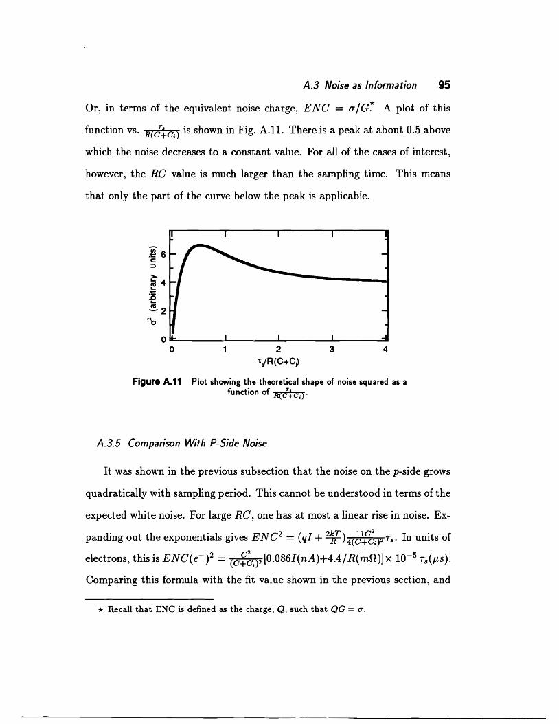
A.3 Noise as Information 95
Or, in terms of the equivalent noise charge, ENC = a /G~ A plot of this
function vs. R(d°.tc.) is shown in Fig. A.11. There is a peak at about 0.5 above
which the noise decreases to a constant value. For all of the cases of interest,
however, the RC value is much larger than the sampling time. This means
that only the part of the curve below the peak is applicable.
Ci) .'!:: 6 c :l
>-~ 4 !: :c ~2
Nt:)
Q...._ ______ _._ ________________ ...... ______ ......iiilil
0 2
'tJR(C+CJ
3 4
Figure A.11 Plot showing the theoretical shape of noise squared as a function of R(d°+ci).
A.3.5 Comparison With P-Side Noise
It was shown in the previous subsection that the noise on the p-side grows
quadratically with sampling period. This cannot be understood in terms of the
expected white noise. For large RC, one has at most a linear rise in noise. Ex
panding out the exponentials gives ENC2 = (ql + ¥)4(b~~i)2 T8 • In units of
electrons, this is ENC(e-)2 = (c~~.)2 [0.086J(nA)+4.4/ R(mO)] x 10-5 r8 (µs).
Comparing this formula with the fit value shown in the previous section, and
* Recall that ENC is defined as the charge, Q, such that QG = u.

96 Cleo-II Silicon Detectors
using the measured leakage current value of 1 nA per strip plus the expected
value of C /( C +Ci) of 0.8, yields a value for the bias resistor of 28!tg Mn.
This is consistent with an independently measured lower limit of 100 Mn at
the level of about 2u because of the highly asymmetric errors. The quadratic
component of the noise is not understood; nevertheless, the large RC value
implies that the spectral power density of the noise source, whatever it is, must
be of the 1 / f form in order to produce a quadratic dependence.
A.3.6 Comparison With N-Side Noise
For the n-side, the noise was found to be consistent with a linear depen
dence on Ts as shown in the previous section. However, the bias resistor was
independently measured to be 3.5 Mn and the capacitance at about 10 pF so
that RC is only about 35 µs. This value of RC is not large enough to justify
using only the linear terms in the noise function. For this reason a fit of the
data was performed using the full noise function. The parameters to be found
were taken to be R(C +Ci), the normalization in front of the above noise
function, and a constant representing the noise that is independent of Ts. The
fit is shown in Fig. A.12. The resulting value of RC was 65!t8 µsand for the
normalization, a value of .95 ± .08. Taki~g C = 11.4 pF from an independent
measurement, and using the measured leakage current of 0.5 nA, one can solve
for the bias resistor and C + Ci. The results are 5!~ Mn and 13!~ pF re
spectively. These results are consistent with the values of 3.5 Mn and 12 pF
obtained in an independent measurement. The fit value of the constant noise
term is 79±5.5 which translates into an ENC of about 500 e-. If this were due

A.4 Summary of Main Noise Results 97
300
250
N-200 0 0 150 ~
"'t> 100
50
0 0 2 3
't.(JJ.S) 4 5
Figure A.12 Fit of noise from then-side of a detector.
6
solely to the capacitance of the detector and taking ENC= 290 + 30C(pF),
then one obtains C = 7.6 ± 0.3 pF. This is higher than the expected value of
about 1 pF. It is not clear what the source of this noise is. It could be within
the detector itself, or it could be that the CAMEX used with this detector (it
was from the new batch of CAMEXes) has a capacitance noise slope that is
much larger than 30 e- /pF. This is currently under investigation.
A.4 Summary of Main Noise Results
A number of techniques have been found which reduce the noise. These
are outlined here together with the magnitude of their effect on the ENC:
• Have time between R2 and Rl greater than 100 µs. {1000 e-)
• Leave the shield of strip cables unconnected. {130 e-)
• Have an RC > 1 Mn x 50 nF = .05 s filter on the bias line to each
detector. (2000 e-)

98 Cleo-I I Silicon Detectors
• Amplify the output before sending it down a long cable. This reduces
pickup and the effects of ground differences between the ADC and the
CAMEX. (100 e-)
With these noise reducing techniques the ENC of a blank CAMEX is about
300 e-. For the new batch of CAMEXes, however, the testpulse lines need
to be grounded or attenuated by a factor of at least 100. With a detector
connected, the noise on the p-side is about 340 e- at a sampling time of
400 ns and grows quadratically with sampling time. This quadratic rise is
indicative of a } current noise source. For the n-side, the noise is about
570 e- at a sampling time of 400 ns and grows linearly with sampling time.
The magnitude of the linear rise is consistent with what would be expected
from the Johnson noise associated with the bias resistor. The excess noise
on then-side compared to the p-side could be due to either unknown sources
within the detector itself, or an unusually large noise vs. input capacitance
slope for the new batch of CAMEXes.

REFERENCES
1. M. Kobayashi and T. Maskawa, Prog. Theor. Phys. 49 (1973), 652.
2. H. Georgi, Weak Interactions and Modern Particle Theory, Benjamin
Cummings, Menlo Park, CA, 1984.
3. M. Aguilar-Benitez et al., Phys. Rev. D45 (1992), Part 2.
4. D. Decamp et al., Phys. Lett. B235 (1990), 399; P. Abreu et al., Phys.
Lett. B241 (1990), 435; B. Adeva et al., Phys. Lett. B237 (1990), 136;
M. Z. Akrawy et al., Phys. Lett. B240 (1990), 497.
5. N. Isgur and M. B. Wise, Phys. Lett. B232 (1989), 113, and B237
(1990), 527; H. Georgi, Phys. Lett. B240 (1990), 447.
6. M.E. Luke, Phys. Lett. B252 (1990), 447; M. Neubert, Phys. Lett. B264
(1991 ), 455.
7. N. Isgur and M. B. Wise, Phys. Rev. D42 (1990), 2388.
8. J. D. Richman Cal. Tech. Preprint CALT-68-1148, 1984.
9. J. R. Raab et al., Phys. Rev. D37 (1988), 2391; J. R. Raab, thesis,
UCSB, 1987.
10. See W. T. Eadie et al., Statistical Methods in Experimental Physics,
Elsevier, New York, 1988.
11. J. C. Anjos et al., Phys. Rev. Lett. 62 (1989), 722.
12. M. Bauer et al., Z. Phys. C34 (1987), 103.
- 99 -

13. The radiative correction has been evaluated by adapting a calculation
for I< e3 decays given by E. S. Ginsberg, Phys. Rev. 142 (1966), 1035.
14. J. Adler et al., Phys. Rev. Lett. 60 (1988), 89.
15. J. R. Raab et al., Phys. Rev. D37 (1988), 2319.
16. J. C. Anjos et al., Phys. Rev. Lett. 62 (1989), 1587.
17. J. C. Anjos et al., Phys. Rev. Lett. 65 (1990), 2630.
18. K. Kodama et al., Phys. Lett. B274 (1992), 246, Carnegie-Mellon
Preprint CMU-HEP92-10.
19. Presented at the "XXVI International Conference on High Energy
Physics," Dallas, TX, 1992.
20. N. Isgur et al., Phys. Rev. D39 (1989), 799.
21. T. Altomari and L. Wolfenstein, Phys. Rev. D37 (1988), 681; plus
F.J. Gilman and R.L. Singleton, Phys. Rev. D41 (1990), 142.
22. M. Wirbel et al., Z. Phys. C29 (1985), 627.
23. J.G. Korner and G.A. Schuler, Z. Phys. C38 (1988), 511.
24. P. Ball et al., Phys. Rev. D44 (1991 ), 3567.
25. T.M. Aliev et al., Trieste preprint IC-89-382.
26. C.W. Bernard et al., Phys. Rev. D45 (1992), 869.
27. V. Lubicz et al., Nucl. Phys. B356 (1991), 301.
28. M. Bauer and M. Wirbel, Z. Phys. C42 (1989), 671.
-100 -

29. D. Scora and N. Isgur, Phys. Rev. D40 (1989), 1491.
30. H. Becker, et al, IEEE Trans. Nucl. Sci. 36 (1988), 246.
31. E. Gatti and P. F. Manfredi, Rivista Del Nuovo Cimento 9 (1986), 1.
32. J. B. Johnson, Phys. Rev. 32 (1928), 97.
33. W. Shottky, Ann. Physik. 57 (1940), 244.
34. W. Butler et. al., M.P.I. Preprint MPI-PAE/Exp. El. 178, 1987.
- 101 -


![The KMI project · 2013-12-13 · The KMI project Yasumichi Aoki [Kobayashi-Maskawa Institute(KMI), Nagoya University] - at KMI2013 International Symposium - Dec. 11, 2013 Kobayashi-Maskawa](https://img.dokumen.tips/doc/110x75/5f624edcf4d4f16dff22e608/the-kmi-2013-12-13-the-kmi-project-yasumichi-aoki-kobayashi-maskawa-institutekmi.jpg)


