i

ii

Professor Peter Cook 84 Richmond Avenue Colonel Light Gardens SA 5041 Pgcook65@gmail.com Professor Derek Eamus School of Life Sciences University of Technology Sydney PO Box 123 Sydney NSW 2007 Derek.Eamus@uts.edu.au Cover Photo: Open woodland vegetation in the Ti Tree Basin.

iii

Table of Contents

Executive Summary .................................................................................................................... v

1. INTRODUCTION ................................................................................................................... 9

2. METHODOLOGIES TO INFER GROUNDWATER USE .......................................................... 11

2.1 Direct Measurements of Rooting Depth 11

2.2 Soil Water Potentials 12

2.3 Leaf and Soil Water Potentials 13

2.4 Stable Isotopes 2H and 18O 14

2.5 Depth of Water Use and Groundwater Access 16

2.6 Green Islands 17

2.7 Transpiration Rates 19

2.8 Tree Rings 20

2.9 Dendrometry 22

2.10 13C of Sapwood 22

3. GROUNDWATER AND VEGETATION IN THE TI TREE BASIN .............................................. 24

3.1 Geography and Climate 24

3.2 Groundwater Resources 27

3.3 Vegetation Across the Ti Tree Basin 29

4. TI TREE BASIN GDE STUDIES ............................................................................................. 32

4.1 Transpiration and Evapotranspiration Rates 32

4.2 Soil Water Potentials 35

4.3 Leaf Water Potentials 38

4.4 Stable Isotopes 43

4.5 Sapwood 13C and Leaf Vein Density 44

5. OTHER ARID ZONE STUDIES .............................................................................................. 48

5.1 Rocky Hill 48

5.2 Pilbara, WA 50

6. OTHER AUSTRALIAN AND INTERNATIONAL STUDIES ....................................................... 52

6.1 Global Rooting Depth Studies 52

iv

6.2 Groundwater Use by Vegetation 56

6.3 Limiting Depths for Vegetation Access of Groundwater 58

7. CONCLUSIONS ................................................................................................................... 61

REFERENCES ............................................................................................................................. 62

APPENDIX 1. MEASUREMENT OF WATER POTENTIAL ............................................................. 71

APPENDIX 2. HYDRUS MODEL OF SOIL WATER FLOW ............................................................. 74

APPENDIX 3. TI TREE VEGETATION SURVEY ............................................................................. 75

APPENDIX 4. GROUNDWATER USE BY VEGETATION IN AUSTRALIA ....................................... 76

v

Executive Summary

Within the past twenty years there has been increased recognition of the need to manage groundwater resources to protect ecosystems that may be dependent on groundwater, as well as to allow productive use of the resource. In arid zones, use of groundwater by vegetation is likely to be much more widespread than in more humid climates, due to the scarcity of other water sources. This can pose difficulties for groundwater managers as groundwater-dependent vegetation can be difficult to distinguish from vegetation that is not groundwater dependent.

A number of methods have been developed for mapping potential groundwater-dependent ecosystems (GDEs) and assessing their groundwater dependence, and these methods fall into two main groups. The first group includes methods that seek to measure the rooting depth of vegetation or the depth of water uptake by vegetation. These include direct measurements of rooting depth from excavation, soil water and leaf water potential measurements, and measurements of the stable isotope composition of groundwater and water within plant xylem. The second group of methods infers groundwater use from relationships between plant condition or plant growth and water availability. Measures of plant condition include indices of ‘greenness’ obtained from remote sensing, or field-based measurements of plant growth (size of annual tree rings or incremental changes in basal area), transpiration or evapotranspiration, or indirect measures of tree stress such as 13C values of sapwood and leaves or leaf vein density.

The Ti Tree Basin has been a focus of groundwater and vegetation studies for almost 20 years, and much of our knowledge of vegetation use of groundwater in central Australia is derived from the Ti Tree studies. These studies have applied most of the methods described above, including measurements of transpiration of individual trees (using sapflow sensors) ecosystem evapotranspiration (using eddy covariance and Bowen Ratio methods), analysis of soil water and leaf water potentials, water isotope (18O) analysis on soil water, groundwater and sapwood, carbon (13C) isotope measurements on sapwood and leaves, and leaf vein density studies. Investigations in open woodland ecosystems in the Ti Tree Basin show use of regional groundwater by a number of different species. In particular:

1) Soil water potential data suggests that many trees have roots concentrated within the top 6 – 8 m of the soil profile, but also provides evidence of water extraction by roots to 15 m depth in areas where water tables are more than 20 m deep. Although a small number of soil profiles indicate water extraction to 20 m depth, a rooting depth of 15 m appears to be more usual in areas with deep water tables. Soil water potential data also indicates water extraction by roots from close to the water table in areas where water tables are 12 m deep or shallower. This indicates that

vi

groundwater use by vegetation may be widespread in areas with water tables less than 12 m depth, but is limited in areas where water tables are deeper than 15 m.

2) Comparison of soil and leaf water potential data indicates water extraction to 15 m depth by Corymbia opaca (Bloodwood) and Hakea macrocarpa (Dogwood Hakea); to 12 m by Acacia melleodora (Scented Wax Wattle) and Eremophylla latrobei (Crimson Turkey Bush); and to 8 m by Acacia aptaneura (Mulga). These species may therefore be groundwater-dependent when the water table is shallower than these depths. Water potential data also indicates water extraction to at least 6.5 m by Acacia maitlandii (Maitland’s Wattle); to 6 m by Acacia coriacea (Dogwood); and to 5 m by Eucalyptus victrix (Smooth-barked Coolibah), Hakea lorea (Bootlace Oak), Acacia victoriae (Bardi Bush) and Acacia bivenosa (Dune Wattle). However, due to limited sampling of these species, they may also be groundwater-dependent in areas with deeper water tables.

3) Water isotope data (18O) provides supporting evidence for extraction of soil water from at least 8 m depth by C. opaca, and also provides evidence of groundwater use by C. opaca and E. camaldulensis (River Red Gum) in areas of shallow water tables.

4) Sapflow data shows that total water use of C. opaca is much greater where water tables are 12 m depth and less, than in areas with water tables 20 m or more. The large difference in transpiration rate suggests that there would be a significant change in tree condition if water tables were lowered from 12 to 20 m.

5) Sapwood 13C and leaf vein density show significant differences in water stress of C. opaca and E. camaldulensis between areas with water tables less than and greater than approximately 10 m depth.

The results show clear evidence of groundwater use throughout the basin in areas with water tables of 12 m or less, and evidence of soil water uptake from 15 m depth in areas where the water table is deeper. Although there is some evidence of soil water use from deeper than 15 m, the volume of groundwater extracted from these depths is likely to be small. C. opaca, which appears to be the most deeply-rooted species, is likely to be using groundwater where it is shallower than 15 m depth. E. camaldulensis also access groundwater, and tend to occur in riparian areas and where perched shallow aquifers are present. In the north of the basin where water tables are 6 m or less, more shallow-rooted species are able to access groundwater, including Eucalyptus victrix. Stirling Swamp is also a GDE, with total annual evapotranspiration from the ecosystem greatly exceeding annual

vii

rainfall. Since this is a water-limited environment, we argue that groundwater use implies groundwater dependence, and removal of access to groundwater will result in a change in vegetation condition.

The Ti Tree results are supported by studies at Rocky Hill, south of Alice Springs, where soil water potential profiles show extraction of soil water to at least 10 m in places, with some evidence of extraction to 20 m; and in the Pilbara, northwestern Australia, where E. victrix has been shown to use groundwater at 6 – 7 m depth. Investigations in less arid sites have found significant differences in transpiration of woodland ecosystems and also measurable differences in ecosystem structure and function where water table depths are in excess of 10 m, compared to areas with shallower water tables.

viii

9

1. INTRODUCTION

Within the past twenty years there has been increased recognition of the need to manage groundwater resources to protect ecosystems that may be dependent on groundwater, as well as to allow productive use of the resource. Groundwater-dependent ecosystems (GDEs) are ecosystems which require access to groundwater on a permanent or intermittent basis to meet all or some of their water requirements so as to maintain their communities of plants and animals, ecological processes and ecosystem services (Richardson et al., 2011). Groundwater-dependence does not mean that the ecosystem will cease to exist if groundwater is removed, but rather that groundwater is important to maintain its current condition, and so if groundwater is removed then the ecosystem will change.

Hatton and Evans (1998) identified four classes of groundwater-dependent ecosystems: vegetation, river base flow systems, aquifer and cave ecosystems and wetlands. Since that time, an additional two classes of GDEs have become apparent: terrestrial fauna, and estuarine and near-shore marine ecosystems (Clifton and Evans, 2001). The importance of groundwater for sustaining ecosystems has been stressed in the scientific literature (e.g., Eamus et al., 2006) and become enshrined in government policy. Water legislation in most Australian states and territories requires that water allocation plans and policies consider the water needs of ecosystems that may be dependent on groundwater. A conceptual framework for management of groundwater-dependent ecosystems (GDEs) has been devised for Australia (Clifton and Evans, 2001), and comprises four steps: (i) identify potential GDEs, (ii) establish the natural water regime of GDEs and their level of dependence on groundwater, (iii) assess the environmental water requirements of GDEs, and (iv) devise water provisions that will deliver these environmental water requirements. Subsequent work has further developed this framework, and also compiled and summarised the various tools that can be used for GDE assessments (Clifton et al., 2009; Richardson et al., 2011). However, despite these efforts, GDE assessments have generally stalled at the first stage of the process, and have not progressed through the three subsequent steps of the conceptual framework. Although a number of techniques are available for determining potential GDEs, establishing the level of dependence of ecosystems on groundwater, and predicting impacts of changed water regimes remain major challenges.

Even if their dependency on groundwater is difficult to establish, some potentially groundwater-dependent ecosystems can readily be identified in the field or using remote techniques. Thus mapping of rivers, wetlands and surface waterholes is relatively straightforward. Vegetation represents a greater challenge, as it can occur across the landscape, rather than at discrete locations. In arid zones, groundwater-dependent vegetation is likely to be much more widespread than in more humid climates, due to the scarcity of other potential water sources. Roots of vegetation have been found as deep as

10

50 – 60 m depth (Le Maitre et al., 1999) and groundwater use by vegetation has been measured from depths in excess of 30 m (Orellana et al., 2012). However, despite the propensity for groundwater use by vegetation, identifying vegetation that is using groundwater and that is dependent on that water source remains a challenge. This report discusses the evidence for groundwater use by vegetation in central Australia, and hence the potential for groundwater-dependent vegetation. It focusses on the Ti Tree Basin, as this area has been a focus for research on groundwater-dependent ecosystems for almost 20 years, but also discusses relevant data from other studies within the Australian arid zone.

11

2. METHODOLOGIES TO INFER GROUNDWATER USE

Methodologies to identify groundwater-dependent vegetation fall into two main categories. The first group of methods seek to measure the rooting depth of vegetation or the depth of water uptake by vegetation. These include direct measurements of rooting depth (Section 2.1), soil water and leaf water potential measurements (Sections 2.2 and 2.3), and measurements of the stable isotope composition (2H, 18O) of groundwater and water in the plant’s xylem (Section 2.4). The second group of methods infers groundwater use from relationships between plant growth and water availability (Osmond et al., 1987; Oberhuber et al., 1998; Sarris et al., 2007). In arid and semi-arid regions those species accessing groundwater may be expected to be very sensitive to increases in groundwater depth, particularly during dry periods when the upper soil water content declines substantially. Measures of plant growth include indices of ‘greenness’ obtained from remote sensing, and this approach usually seeks to identify vegetation that remains ‘healthy’ during times of low rainfall (Section 2.6). Field-based studies that measure vegetation growth indicators or tree condition include measurements of transpiration or evapotranspiration (Section 2.7), tree ring studies (Section 2.8), dendrometry (Section 2.9) and 13C values of sapwood and leaves (Section 2.10). All of these methods have application to the Australian arid zone, and many have already been applied in studies within the Ti Tree Basin.

2.1 Direct Measurements of Rooting Depth

Knowledge about root depth of vegetation is extremely valuable in the study of groundwater-dependence. The most common method for obtaining such data is from trenches. Logarithmic spiral (Atkinson and Dawson 2000), semi-circular (Grant et al., 2012) or rectangular (Macinnis-Ng et al., 2010) trenches can be excavated, and can be dug by hand or using a backhoe to depths ranging from 0.1 – 10 m. However, deep trenches require significant consideration of safety due to the potential for the sides to cave inwards.

Clearly the depth of the trench sets the upper limit for the maximum depth to which roots can be observed. The optimum depth is a trench that either reaches the water table, or, which exceeds the depth of the roots, whichever is the deeper. Trenching to the water table and examination for roots provides absolute evidence of the presence/absence of interaction of roots with the capillary fringe of the aquifer. If the desired information pertains merely to root depth, the presence/absence of roots on the cut faces of the trench is recorded as a function of depth. If information about root length/biomass distribution as a function of depth are required, root length distribution can be estimated using the modified Newman line intersect method (Newman 1966) whereby the length of a root

12

visible is a function of the number of lines on a grid intersected by the root. In addition, replicate shallow cores of known depth can be inserted into the exposed face at a number of depths and locations, the soil extracted and then sorted for roots within the known volume of soil and biomass estimated by drying (Macinnis-Ng et al., 2010).

Root coring by hand is possible where soil structure permits and where depths are not excessive. Where depths exceed what is manually possible, or soil structure prohibits, mechanical coring using steel corers with hardened cutting teeth attached to a suitable drive mechanism is required. The presence/absence of roots in the extracted core is recorded as a function of depth. The advantage of coring over trenching is the possibility of increased sample numbers (i.e., replication). Whilst most studies report an exponential decline in root biomass as a function of depth, bimorphic distributions are also encountered, in which there is a profusion of root biomass at depth, just above the water table (Canham et al. 2012).

Another technique that can be used to obtain information on root distribution is ground penetrating radar (GPR), which uses radar pulses to interrogate the regolith. Reflections of the radar pulses occur at electromagnetic discontinuities within the regolith, including at the surface of roots, bedrock and the water table (Lorenzo et al., 2010). It is non-destructive and may be able to provide estimates of root depth and root distribution.

2.2 Soil Water Potentials

The soil water potential is a measure of the pressure with which moisture is held by the soil, and hence the difficulty of the vegetation extracting it. It is the sum of the matric potential (due to the forces of capillarity and surface adsorption) and the osmotic potential (due to the presence of solutes within soil water). By convention, matric potentials are negative, with drier soils (where the water is more tightly held) more negative. A saturated soil has a matric potential of zero, but can have a negative osmotic potential and hence negative water potential due to the presence of dissolved salts. However, in a dry soil with relatively low salt content, the water potential will be approximately equal to the matric potential.

Total potential is the sum of water potential and gravitational potential, and water flow occurs only in response to gradients in total potential. Relatively high gradients in total potential thus indicate relatively high rates of flow. Changes in the total potential gradient with depth can indicate the base of the plant root zone, or at least a decrease in the rate of vegetation water uptake.

Strong gradients in soil matric potential or water potential will usually only exist immediately below zones of active water extraction. In the absence of root extraction,

13

water is lost from the soil surface by evaporation, and the profile of both soil matric potential and water potential in a dry soil will usually be most negative at the soil surface (where water is lost by evaporation) will increase approximately exponentially with depth. However, where roots occur within the profile, the base of the root zone can sometimes be identified by rapid increases in both soil matric potential and soil water potential (Figure 1). However, care is needed to avoid drying the soil during sample collection, particularly using motorized drill rigs (Cook et al., 2008). Hand auguring is preferred for this reason, but is not feasible in many areas.

Figure 1. Matric potential profile measured beneath native mallee vegetation near Euston, southwestern NSW. The water table occurs at approximately 20 m, and low matric suctions to below 13 m indicate that roots are extracting soil water to at least this depth. (Note that matric suction is the absolute value of matric potential.) After Cook and Walker (1989).

2.3 Leaf and Soil Water Potentials

Leaf water potentials reflect the water status of a leaf, a canopy and a plant. Water potentials are either zero (well-watered soil, leaves measured on a cool night) or negative. The more negative the value, the more likely the plant is experiencing water stress, although very large variation exists across species as to what value of water potential represents early, mid- and late stages of water stress. A crop such as cotton may exhibit a midday leaf water potential of -1.0 MPa on a warm sunny day with wet soil and will be considered not water stressed. However, at –2.5 MPa the same plant is experiencing severe water stress. In contrast, Acacia aptaneura (Mulga) can experience a midday water

14

potential of -4.5 MPa and not be stressed (as evidenced by wide open stomata and a high rate of photosynthesis).

Water potentials are routinely measured at predawn and midday. Predawn water potential is taken as a reasonable approximation of the water potential of the soil within the root zone where a significant fraction of the roots are found. Overnight, canopy (and hence leaf) water potentials increase towards zero as stem and canopy rehydration occurs. Once the canopy and root zone soil water potential are at equilibrium further increases in leaf water potential are precluded. At midday leaf water potential is at, or approaching, a daily minimum.

Leaf water potentials provide information on depths of water uptake by vegetation. Vegetation can only extract water from depths where the soil water potential is greater than the minimum leaf water potential that is achieved during the day. This will create a gradient for water to move upwards through the plant xylem to the leaf, where it is evaporated at the leaf surface. As soil water potentials generally increase with depth, the maximum leaf water potential will often define the minimum rooting depth of the vegetation.

There are two common methods for measuring leaf or stem water potential: pressure chambers and thermocouple psychrometers. A third, relatively new technique is the cooled mirror dewpoint hygrometer. These methods are described in Appendix 1.

2.4 Stable Isotopes 2H and 18O

Deuterium (2H) and oxygen-18 (18O) ratios can be used to estimate the depth from which water is being extracted by comparing the isotope signatures of groundwater, soil water at multiple depths through the profile, and water in plant xylem (Thorburn et al., 1993; Zencich et al., 2002; Lamontagne et al. 2005; O’Grady et al., 2006; Kray et al., 2012). If there is sufficient difference in the isotope signatures of groundwater and soil water, then analyses of xylem water can provide an estimate of the depth of extraction of water and the proportional contribution of groundwater and soil water to transpired water. The principal of the method is illustrated in Figure 2. Examples of the use of 2H and/or 18O to discriminate water sources include identification of soil and surface water use by juvenile riparian plants, in contrast to groundwater use by mature trees (Dawson and Ehleringer, 1991), and determination of the mountainous source of groundwater and opportunistic use of that groundwater by riparian trees (Chimner and Cooper, 2004). Of course, this method does not always work, and requires a clear difference between soil and groundwater isotope compositions for this method to be successful. It can also sometimes suffer from lack of

15

replication, as deep profiles of the stable isotope of soil water can be difficult to obtain and stable isotope values can be spatially variable.

Figure 2. Hypothetical example of vertical profile of deuterium (2H) in soil water. Within the unsaturated zone, the 2H value decreases linearly from -30 to -10 ‰, and within the groundwater it is uniform at -10 ‰. A measured value of -10 ‰ for leaf xylem water would therefore indicate groundwater use. Values less than -10 ‰ would indicate soil water use, with lower values indicating that plants are extracting water from closer to the soil surface.

In addition to using isotopes of water to identify the utilisation of groundwater by vegetation, it is possible to estimate the relative contribution of multiple sources of water to the total water absorbed by roots using mixed-member models (i.e., “Keeling plots”) (Phillips and Greg 2003). While theoretically possible for linear mixing models to distinguish more than two potential sources of water, such an application requires the fractionation of 2H or 18O to be independent of each other, which is often not the case. At a minimum, though, the use of stable isotopes can provide information about spatial and temporal variation in groundwater dependency across species and ecosystems.

Cook and O’Grady (2006) have developed a model that estimates the relative water uptake by vegetation from different soil depths. In their model, the rate of water uptake is determined by (a) gradients in water potential between soil and canopy; (b) the distribution of roots through the soil profile; and (c) a lumped hydraulic conductance parameter. Soil isotopic composition at different soil depths and also of xylem water is used to constrain root distributions within the model. This has the distinct advantage over end-member

16

analyses (see above: an analytic tool to determine the relative contributions of soil water and groundwater to transpiration; Phillips and Gregg 2003) because: (i) it produces a quantitative proportional estimation of water extracted from multiple depths (including groundwater); (ii) it doesn’t require distinct values of isotope composition for end-member analyses (which is frequently not observed) and therefore can deal with the more typical grading of isotope composition observed through the soil profile; and (iii) it is based on simple ecophysiological principles. Cook and O’Grady (2006) applied this model and demonstrated that for two co-occurring species, 7–15 % of their transpired water was sourced from groundwater while a third species accessed 100 % from groundwater. A fourth species derived 53–77 % from groundwater.

To estimate the groundwater use by vegetation an independent estimate of ET0 or ETa derived from eddy covariance (Baldocchi and Ryu, 2011), sapflow (O'Grady et al., 2006; Zeppel, 2013) or remote sensing techniques (Nagler et al., 2013) is required, in addition to the stable isotope composition of water in soil, groundwater and xylem. Upon determination of the proportion of ET that is due to ETg (itself a complex process, see Eamus et al., 2015 for a review of this), the amount of ETg, is then the product of that proportion and ET.

2.5 Depth of Water Use and Groundwater Access

Most of the above techniques seek to identify the depth below the surface where water is extracted. However, establishing that vegetation is extracting water from the unsaturated zone does not exclude the possibility that this water is ultimately derived from the groundwater. Given sufficient time, soil water potentials of -2 MPa and less will induce upward movement of water from water tables in excess of 200 m below. The question, rather, is whether the water used by the vegetation is replenished by downward percolation of rainfall infiltration, or upward movement of groundwater from the water table.

Of course, where the distance between the base of the root zone and the water table is large, the volume of groundwater that can potentially be extracted is likely to be relatively low. Figure 3 shows the upward groundwater flux that would occur under steady state conditions for distances between the base of the root zone and the water table, and assuming a water potential within the root zone of -40 MPa. Where roots extend to within 1 m of the water table, upward water fluxes of more than 10 mm y-1 will occur for all except very sandy soils. For relatively fine textured soils, such as clay loams and silty clay loams, upward fluxes of more than 1 mm y-1 can occur even where the base of the root zone is more than 10 m above the water table. This can be significant for the groundwater balance

17

in arid regions, although it isn’t significant in terms of plant water relations or vegetation water use.

Figure 3. Numerical simulations of the maximum groundwater flux that can be sustained from root extraction from the unsaturated zone, as a function of distance between the base of the root zone and the water table and soil type. The modelling approach is described in Appendix 2.

2.6 Green Islands

Remote sensing (RS) of vegetation structure and function (especially leaf area index, vegetation water use and productivity) is now common (Ma et al., 2013; Nagler et al., 2013) and can be applied to vegetation and water resource management (Doody et al., 2014). “Green Islands” is a concept describing the application of RS for identification of the location and functioning of GDEs (Everitt and DeLoach, 1990; Akasheh et al., 2008). In this method, the attributes of one pixel in an RS image are compared to those of another pixel located nearby. If one pixel contains a GDE but the other does not, the structure and function of vegetation in the two pixels may differ during periods of water shortage because vegetation with groundwater access will not be subject to the same degree of soil water deficit as vegetation that does not have groundwater access. By comparing pixels across relatively

18

wet and relatively dry periods, “green islands” within a sea of browning vegetation can be identified (Contreras et al., 2011).

Munch and Conrad (2007) used Landsat imagery to identify the presence/absence of wetlands across three catchments in South Africa. GIS terrain modelling was combined with RS images to identify the location of GDEs using a landscape “wetness potential” for GDEs reliant on surface expression of groundwater. After combining this with a GIS model of landscape characteristics, they produced a regional-scale map of GDE distributions.

In arid and semi-arid regions, plant density (stems per hectare) is frequently correlated with water availability (plant density is larger when groundwater is available than when it is not). Lv et al. (2012) used the normalised difference vegetation index (NDVI), to examine changes in vegetation structure (which includes a measure of plant density) as a function of depth to groundwater. NDVI is a measure of the “greenness” of canopies (Huete et al., 2002). Using a high resolution (25 m) digital elevation model and groundwater depth data, a relationship between NDVI and depth-to-groundwater was established (Figure 4).

Figure 4. The relationship between NDVI and depth to the water table for the Hailiutu River catchment in northern China. Redrawn from Lv et al. (2012).

Lv et al. (2012) found that NDVI was most sensitive to water table depth where the water table was within 10 m of the land surface, and that vegetation cover was relatively insensitive to increases in groundwater depth beyond 10 m. In contrast, a threshold of approximately 4.4 m depth was identified in the Ejina area of NW China (Jin et al., 2011). In their study, in a region where annual rainfall was about 40 mm, vegetation was absent in regions where groundwater depth exceeded 5.5 m. Maximal NDVI values were recorded at sites with intermediate (2.5 – 3.5 m) depth-to-groundwater rather than at sites with shallower groundwater. This may have arisen because of the effects of anoxia arising from

-100

-80

-60

-40

-20

00 0.2 0.4 0.6 0.8

Dept

h of

the

wat

er

tabl

e (m

)

NDVI

19

root flooding when the water table is too shallow (Naumburg et al., 2005; Zolfaghar et al., 2016).

Ecological, hydrological and geological data can be combined to define regions having common physical and climatic envelopes. Within unmanaged vegetation, similar vegetation cover may be expected within these regions, and thus similar RS attributes are expected. Dresel et al., (2010) used this methodology in South Australia and developed a correlation analysis using Landsat summer NDVI and MODIS enhanced vegetation index (EVI). MODIS EVI images were used to identify regions displaying reasonably consistent photosynthetic activity throughout the year. Landsat NDVI images were then used to locate areas displaying large inter-annual variation in photosynthetic activity across wet and dry years. They then used a classification of Landsat spectral data to identify pixels with similar spectral signatures of known groundwater-dependent ecosystems. Dresel et al. (2010) were able to identify all pixels across a catchment that had a very high probability of being a GDE. Significant ground truthing was required to assess the validity of this method.

An alternative approach to locating GDEs relies on mapping of groundwater discharge zones. Discharge of groundwater can have significant effects on local ecology. Geological, hydrological, ecological and climate data are required (Tweed et al., 2007). Leblanc et al. (2003a, b) used thermal, Landsat optical and MODIS NDVI data coupled to digital elevation models and depth-to-groundwater data, to locate discharge areas in the semi-arid Lake Chad basin of Africa. Similarly Tweed et al., (2007) examined discharge in the Glenelg-Hopkins catchment of SE Australia. They observed low variability of vegetation activity across wet and dry periods using NDVI. Variability in NDVI was correlated with locations where groundwater was supporting vegetation activity. This method tends to be most accurate in more xeric locations, where rainfall is more likely to limit vegetation function.

Access to groundwater results in a larger leaf area index (LAI), basal area or growth increment than similar sites (in terms of rainfall and species composition) lacking access to ground water and these differences have been used to identify the location of groundwater-dependent vegetation (Benyon and Doody 2004; Zolfaghar et al. 2016, O’Grady et al., 2010).

2.7 Transpiration Rates

Evapotranspiration rates over large areas can be measured using Bowen Ratio and Eddy Covariance methods, and transpiration rates of woody vegetation can be measured using sapflow sensors (Zolfaghar et al., 2017).

20

Long-term evapotranspiration rates larger than rainfall over the same time period indicates that ecosystems have access to an additional water source. In areas that do not received surface run-on, this is likely to be groundwater. Thus, Polglase and Benyon (2008) identify several sites in SA, NSW and WA where annual rates of transpiration of plantations of E. globulis (Blue Gum), Pinus radiata (Radiata Pine), Corymbia maculata (Spotted Gum) and E. kochii (Oil Mallee) greatly exceed annual rates of rainfall. Of course, measurements need to be made over sufficiently long period of time (annual or longer), to ensure that soil moisture carried over from one hydrological year to the next is not the additional source.

Often transpiration is measured from only selected species, and so transpiration will only represent a small proportion of ecosystem water use. In this case transpiration rates are unlikely to exceed rainfall, even though vegetation may be accessing groundwater. Nevertheless, information on groundwater access can be obtained from differences in transpiration between wet and dry periods, based on the assumption that transpiration of trees with groundwater access will be less affected by period of low rainfall than those without such access. Some studies have also attempted to establish relationships between transpiration rate and water table depth to establish groundwater use (e.g., Howe et al., 2007; Zolfaghar et al., 2017).

An important technique that offers the potential to independently determine rates of transpiration loss from groundwater involves interpretation of diurnal patterns in water table depth. If vegetation are extracting water from the saturated zone, then the groundwater level would be expected to decline during the day, but to “rebound” at night when transpiration ceases (or at least reduces). This pattern, if present, results in a sinusoidal signal in the local groundwater level that has been used to calculate phreatophytic ET (White, 1932; Lautz, 2008).

2.8 Tree Rings

Dendrochronology (the study of tree growth through analyses of tree rings) has been used in ecological research for many decades (Drew and Downes 2009). However, its application to the study of groundwater dependence is more recent (e.g. Giantomasi et al., 2012).

Tree rings record the history of past growth. In Europe and the USA growth is strongly seasonal and generally predictable, allowing tree rings to record annual cycles. Determination of growth rates from annual tree rings (and dendrometer records; see Section 2.9) can establish relationships among water supply, including fluctuations in water supply from precipitation and groundwater (Bogino and Jobbagy, 2011; Perez-Valdivia and Sauchyn, 2011; Xiao et al., 2014), and temperature. Patterns in tree ring growth and

21

patterns in depth to groundwater can also be correlated, in some locations, to the dominant regional driver of climate, such as the El Niño–Southern Oscillation in California, USA (Hanson et al., 2006). Spectral analyses can sometimes disentangle the interactions of climate from groundwater supply (Bogino and Jobbagy, 2011) but in other cases groundwater depth was not found to be important in explaining differences in either ring width or basal area increment (Stock et al., 2012). Seasonal changes in the magnitude of groundwater use can influence the degree to which a climate signal can be observed in patterns in tree rings: climate signals can be weaker during formation of late wood, when growth rates are small (Oberhuber et al., 1998), or during the dry season, when precipitation is minimal and growth is more dependent on groundwater (Drake and Franks, 2003).

Thus, tree ring chronologies can provide insights into the importance of access to groundwater on plant growth. Individual events can be identified in chronologies of tree rings (Hultine et al., 2010). Furthermore the impact of longer-term trends in depth-to-groundwater can sometimes be determined (Bogino and Jobbagy, 2011). Hultine et al. (2010) was able to identify large, rapid and reversible responses in tree ring width of cottonwood and willow trees in response to draining and refilling of a reservoir.

Whilst it is true that tree rings are rarely observed in Australian tree species, the principle that stem increment may reflect water availability potentially provides an important monitoring approach. Reduced rates of stem growth following groundwater extraction (Lageard and Drew, 2008) and increasing growth rates with decreasing depth-to-groundwater have been observed, although root anoxia can reduce growth rates in response to reduced depth to groundwater (Bogino and Jobbagy, 2011). However, specific responses depend upon multiple factors, which are likely to include the following:

• depth-to-groundwater at the start of the change in depth-to-groundwater; • rate of change of depth-to-groundwater; • duration of change in depth-to-groundwater; • plant functional type and species; • recent decadal trends in depth-to-climate • climate

Identifying and contrasting the sensitivity of species and vegetation communities to meteorological drought (reduced rainfall coupled with increased vapour pressure deficit (VPD) and temperature) compared to “groundwater drought” (that is, increased depth-to-groundwater) are valuable for development of an understanding of relationships among climate, groundwater and groundwater dependent vegetation.

22

2.9 Dendrometry

Whilst the majority of Australian tree species do not show reliable annual tree rings, the use of recording dendrometers (i.e., dendrometers attached to data-loggers) is likely to represent a significant technology for application in studies of groundwater dependent vegetation in the near-future. The relationship between groundwater availability and tree rings observed by Hultine et al. (2010) in cottonwood and willow trees would also have been detectable in long-term dendrometer records had they been available.

On small time-scales (sub-hourly-to-daily), the growth (and shrinkage) of tree stems can be measured and recorded using precision dendrometers. Such dendrometers contain linear-variable-displacement transducers (Zweifel et al., 2005, Drew et al., 2008, Drew and Downes 2009). They can be used to examine relationships among weather variables, soil moisture content and stem diameter increment. Changes in maximum daily trunk shrinkage arising from reduced water availability occur earlier and more strongly than reductions in stomatal conductance, stem water potential or transpiration (Conejero et al., 2007, 2011; Galindo et al., 2013). February et al. (2007) and Drake et al. (2013) found that increased groundwater supply (actual or simulated) results in increased stem increment, xylem sapflow (tree water use) and xylem water potential.

2.10 13C of Sapwood

Wood laid down during periods of drought (meteorological or groundwater drought) is enriched in the stable isotope 13C because of reduced stomatal conductance relative to photosynthesis (Cocozza et al., 2011; Maguas et al., 2011). Although interpretation of δ13C (the 13C isotopic signature) in tree rings can be complicated by the effects of phloem loading of sugars and by photosynthetic re-fixation in the bark of some tree species, wood δ13C can explain differences in groundwater use and water stress in groundwater-dependent trees. Thus δ13C was constant across sapwood from Populus along a perennial stream (thereby implying continuous access to groundwater) but changed with soil moisture conditions in an intermittent reach (because the supply of groundwater and soil moisture varied with time; Potts and Williams, 2004). Similarly, changes in ring width over time were reflected in changes in δ 13C from leaves (Hultine et al., 2010), such that less negative values of δ13C indicated increased water-use-efficiency when water supply declined.

We are aware of only one study that has examined δ13C in wood of Australian species in the context of groundwater depth (Zolfaghar et al., 2014). This study was undertaken in NSW in a mesic Eucalypt woodland across 6 sites where depth-to-groundwater ranged between approximately 2.4 m and 37.5 m. They found significant increases in δ13C of sapwood across

23

five of the six sites, reflecting increasing water-use efficiency as depth-to-groundwater increased. As depth-to-groundwater increases, supply of groundwater declines and increased water-use-efficiency is to be expected.

24

3. GROUNDWATER AND VEGETATION IN THE TI TREE BASIN

Much of our knowledge of groundwater-dependence of arid zone vegetation derives from research in the Ti Tree Basin. This chapter therefore contains a short summary of the geography, climate and groundwater resources of the basin, and the distribution of different vegetation types. Evidence for groundwater-dependence of vegetation within the basin is described in Chapter 4.

3.1 Geography and Climate

The Ti Tree Basin is located approximately 150 km north of Alice Springs, and covers an area of approximately 5500 km2 (Figure 5). The basin is typified by gently undulating sand plains of aeolian origin with alluvial deposits along ephemeral drainage lines. The basin sediments comprise a sequence of gravels, silts, sands and clays up to 300 m thick, with the upper layer of riverine sands forming the main regional aquifer. The main surface water features are Woodforde River and Allungra Creek, in the south (both ephemeral), and Stirling Swamp, in the north. Woodforde River and Allungra Creek have well-defined channels where they enter the basin from the hills to the south, but the channels become less distinct further north, where flow is discharged onto the plains. These surface water discharge areas are known locally as floodouts (Tooth, 1999). Both creeks are highly ephemeral, and at the Woodforde River gauging station, flow events occur on average twice per year, with flow durations typically of a few days to a few weeks (Villeneuve et al., 2015). Stirling Swamp is a large flat salt pan or playa in the northern part of the basin, which becomes inundated after heavy rains.

25

Figure 5. Surface water and groundwater resources of the Ti Tree Basin. From Wood et al. (2017).

Mean annual rainfall in the basin is approximately 320 mm (317 mm at Territory Grape Farm) and potential evaporation (Class A pan) is approximately 3100 mm/y (Jeffrey et al., 2001). However, annual rainfall is highly variable, ranging from less than 100 mm/y to more than 700 mm/y at Territory Grape Farm, over the 26 years of record (1987 - 2013; Station 015643). Long-term rainfall records are available for Barrow Creek, approximately 30 km north of the basin, and for Aileron, approximately 10 km to the south. The mean annual rainfall is 316 mm at Barrow Creek (1874 – 2004) and 302 mm at Aileron (1949 – 2004). Figure 4 shows the recurrence interval of daily rainfall for Barrow Creek and Aileron. On average, daily rainfall totals in excess of 50 mm occur once per year, while daily totals in excess of 100 mm occur once every 10 years. Daily rainfall in excess of 200 mm has been recorded at Barrow Creek on two occasions since measurements were taken. These occurred in 1904 and in 1991. On the latter occasion, 354 mm were recorded over the seven day period (5-11 February). These high rainfall events usually occur in summer, and mean

26

monthly rainfall is highest in February (68 mm) and lowest in July (4.5 mm). Mean daily maximum temperature is 37.5 °C in January and 22.2 °C in June (BOM, 2013).

Figure 6. Mean monthly rainfall (hachured bars) and pan evapotranspiration (solid line) at Barrow Creek (1874-2004). Error bars indicate 1st and 9th deciles of monthly rainfall.

Figure 7. Recurrence interval of daily rainfall for long term records at Aileron (1949-2004) and Barrow Creek (1874-2004).

27

3.2 Groundwater Resources

The thickness of the main unconfined aquifer ranges from < 10 m to approximately 70 m thick (Read and Tickell, 2007), and hydraulic head maps indicate a general direction of groundwater flow from south to north. The depth to groundwater decreases from ~ 50 m in the southwest and southeast corners of the basin, to less than 2 m in the north of the basin, where groundwater discharge occurs by direct evaporation. Groundwater salinities range from less than 1000 mg/L in central parts of the basin, to more than 5000 mg/L in the northern discharge area.

Groundwater recharge has been investigated at specific field sites within the basin, and also using a numerical groundwater flow model. The mean basin-wide recharge rate was estimated to be between 0.07 and 0.7 mm/y using the numerical groundwater model, with a best estimate of 1.1 mm/y. This is in good agreement with the average of 0.8 mm/y reported by Harrington et al. (2002) using the chloride mass balance method. 18O and 2H values in groundwater are consistent with most aquifer recharge occurring from large rainfall events, which occur only every few years (Harrington et al., 1999).

As in most arid regions, groundwater recharge is highly variable spatially, and in the Ti Tree Basin is thought to occur as infiltration of flood flows associated with the ephemeral streams and their floodouts, and also as mountain front recharge following runoff from upland areas that form the basin margin. However, these processes are not well understood. Investigations along the Woodforde River have revealed the presence of a perched aquifer (Villeneuve et al., 2015). The perched aquifer is filled during stream flow events (following infrequent very large rainfall events), and provides a source of water for riparian vegetation between these times, and some of this water leaks down into the regional aquifer. However, recharge from infiltration in river floodouts, which occur downstream of the channelized portions of the rivers, are believed to be more significant. A numerical groundwater model calibrated to hydraulic head and 14C data (Wood et al., 2017) did not find either Woodforde River or Allungra Creek to be major recharge sources, although a zone of high recharge was associated with the floodout downstream of the channelized section of Allungra Creek (see Zone 9 in Figure 8).

Recharge associated with runoff from upland areas surrounding the basin has also been identified based on rapid response of groundwater to rainfall in these areas. The numerical groundwater model identifies mountain front recharge as important, particularly in the southern margin of the basin. Thus recharge rates through zones 1, 3 and 4 are estimated to be 10, 8 and 4 mm/y, respectively (Figure 8).

Recharge in flat sandplains of the basin is believed to be low under present day climate. O’Grady et al. (2007) used a simple soil water balance model using daily precipitation data

28

for Barrow Creek between 1889 and 2005 to examine the relationship between plant root depth and groundwater recharge rate in the Ti Tree Basin. Based on soil moisture deficit within plant root zone of 75 mm per metre depth, the mean drainage rate beneath the a 6 m deep root zone was estimated to be less than 1 mm/year over the 116 year period for which rainfall data were available. For root depths exceeding 7 m, the soil moisture deficit would not have been exceeded within the 116 year period, and so no recharge would have occurred. Since groundwater depths throughout most of the Ti Tree Basin are in excess of 7 m, this suggests that recharge is not occurring under present day conditions. Relatively low chloride concentrations within deep soil profiles, however, indicate that extreme rain events that occur on timescales of several hundred years must infiltrate to water table. In intervening periods, groundwater discharge may be occurring, and over long time periods the rate of groundwater discharge may exceed the rate of recharge. This is supported by results of the numerical groundwater model, which suggests that it is possible that diffuse discharge is occurring over much of the basin, at rates up to approximately 1 mm/y. For rooting depths of 4 – 5 m, recharge events were estimated to only occur on timescales of decades, with groundwater discharge occurring in intervening periods.

Figure 8. Estimated recharge rates for recharge zones used in the groundwater model of Wood et al. (2015). Symbols denote best estimates of recharge and vertical bars denote uncertainties. Zone 13 represents the Woodforde River, and Zone 12 represents Allungra Creek. Zone 9 is the inferred floodout zone from Allungra Creek, and was identified as having the highest recharge rate in the basin.

Groundwater discharge also occurs as evapotranspiration from shallow water tables in Stirling Swamp. Water loss from the swamp was estimated by four different methods, including Bowen Ratio energy balance, chloride and stable isotope profiling, changes in

29

groundwater levels, and 14C profiles within the aquifer (Shanafield et al., 2015). These methods measure discharge at different spatial and temporal scales, and have different assumptions. Although the different methods provided different estimates of groundwater discharge, all estimates were significantly less than estimated recharge for the basin. This suggests that Stirling Swamp is not the main discharge point for the basin, and that other mechanisms of groundwater discharge must be occurring, with discharge through transpiration of deep rooted trees a likely process.

3.3 Vegetation Across the Ti Tree Basin

Three main vegetation ecosystems occur across the Ti Tree Basin. The sand plains of the basin are mostly occupied by Corymbia open woodland, dominated by tall (> 10 m), isolated Corymbia opaca (Bloodwood) trees in the overstory and Spinifex (Triodia) grasses in the understory. Hakea macrocarpa (Dogwood Hakea) and Eucalyptus victrix (Smooth-barked Coolibah) woodlands are also present, along with patches of mono- specific Acacia aptaneura (previously called A. aneura1, a species of Mulga) and isolated Acacia melleodora (Scented Wax Wattle) and A. murryana (Colony Wattle) as scattered shrubs (Nolan et al. 2017).

Riparian forest, primarily consisting of Eucalytpus camaldulensis (River Red Gum) occurs as a narrow corridor along the length of the Woodforde River (typically < 20 m width on either side of the river), and in paleochannels of the river. In these areas a perched aquifer occurs at approximately 2 – 4 m below the surface. Occasionally Acacia estrophiolata occurs in the riparian zone, and Acacia cambegei (Gidgee) occurs as scattered trees adjacent to, but outside of, the riparian zone.

Stirling Swamp generally consists of bare soil, with patches of low-lying vegetation appearing seasonally, including salt tolerant Frankenia (heath) species and Marsilea hirsute, a freshwater fern. The entire Swamp is flooded with water after intense rainfall events (usually during the summer). Groundwater depth is typically between about 1 and 3 m.

M Hingee, a PhD student at UTS undertook a survey of plant species at 10 sites across the Ti Tree (Figure 9). These sites extend across a gradient of groundwater depths, with the shallowest site having a groundwater depth of approximately 3 m at Stirling Swamp and the deepest with a depth to groundwater of approximately 50 m. A total of 38 plant species, comprised of grasses, forbs, shrubs and trees were identified (see Appendix 3 for a full list). Previous studies in arid environments have shown that perennials are selected against

1 A number of the diagrams in this report have been reproduced from earlier papers and reports. Some of these use the old name, A.aneura. Throughout the text, however, we use the new name A. aptaneura.

30

because of their low probability of surviving extended drought periods (Ehleringer 1985). Similarly studies from the arid-zone in South Africa have established that perennials dominate at mesic sites receiving higher rainfall. A short life cycle (e.g. annuals and ephemerals) is an important strategy utilised by many plant species as a means of dealing with long dry seasons. In arid and semi-arid environments following rainfall events, annual plant species are capable of utilising short pulses of soil moisture by germinating, growing and reproducing rapidly. Key results from the Hingee survey are:

a) Total plant abundance (density), species richness, and species diversity, were all

related significantly and independently to one or more of groundwater depth and environmental (soil) Principal Components. High total plant abundance occurred at sites with shallow groundwater depth.

b) Plant longevity was significantly and independently correlated with depth-to-groundwater. Thus, as depth-to-groundwater increased the proportion of perennial species increased and the proportion of annual species decreased (Figure 10). Only one annual species occurred at the deepest sites, and this species (Aristida holathera) was the only one found at all ten sites.

c) Plant growth form was significantly and uniquely related to DGW. More shrub species were found at deep groundwater sites than at shallow sites.

Figure 9. Approximate location of the 10 sites sampled by M Hingee across the Ti Tree Basin.

31

Figure 10. The relative distributions of annual (black) and perennial (grey) species among sites. Sites 1 – 10 are sites of increasing depth to groundwater.

0.00

0.25

0.50

0.75

1.00

1 2 3 4 5 6 7 8 9 10Sites

Prop

ortio

n of

spe

cies

32

4. TI TREE BASIN GDE STUDIES

4.1 Transpiration and Evapotranspiration Rates

Transpiration and evapotranspiration rates in the Ti Tree Basin have been estimated using sapflow, eddy covariance and Bowen Ratio methods.

Initial investigations (in March 2005) used sapflow techniques and focussed on three sites along a 15 km east-west transect in the central part of the basin. Along this transect, the land surface falls towards the east, so that the site on the western edge of the transect (Site 1) has a water table depth of approximately 20 m, while that on the eastern edge (Site 3) has a water table depth of approximately 7.5 m. (Site 2 is midway along the transect, and has a water table depth of approximately 12 m.) Along this transect, vegetation is predominantly an open woodland of Acacia coriacea (Dogwood), H. macrocarpa and C. opaca, with scattered patches of dense A. aptaneura. Site 4 is located approximately 7 km west of this transect, where the water table occurs 30 – 40 m depth. (Documentation is unclear whether the water table at Site 4 occurs at 30 or 40 m depth.) An additional site (Site 5), located approximately 50 km northeast of the other sites, has a water table depth of 5.6 m. At this latter site, E. victrix is co-dominant with C. opaca (Howe et al., 2007).

A subsequent investigation in 2006 (Cook et al., 2008) provided additional measurements of water use at Site 5, and also measured water use of A. aptaneura and E. camaldulensis at a site further west (adjacent to the Woodforde River, and approximately 2 km northeast of Arden Soak). At the latter site, the regional groundwater occurred at approximately 40 m depth, but close to the Woodforde River a perched aquifer was present at approximately 5 m depth. Measurements were made in April and November, these two months reflecting periods of relatively high and low soil moisture availability, respectively. Measurements on E. camaldulensis were made close to the Woodforde River, where the perched aquifer was present, while measurements on A. aptaneura were made approximately 750 m east of the river where the perched aquifer was not present.

Daily water use of three individuals of C. opaca from each site on the transect was measured over a 9 day period in March 2005. Daily water use expressed on a sapwood area basis was highest at Sites 2 and 3 and lowest at Sites 1 and 4. The relationship between mean daily water use and water table depth (Figure 11), would therefore appear to suggest that C. opaca is drawing a significant proportion of its water from groundwater where this occurs at 12 m or less, but may not be accessing groundwater at 20 m depth. Water use within sites showed considerable variability, which led the authors to suggest that increased replication was necessary to unequivocally establish relationships between water table depth and water use.

33

At Site 5, water use was measured in four individuals of each of E. victrix, C. opaca and A. aptaneura using sapflow sensors over a three day period in March 2005. Rates of tree water use were highest in E. victrix, lowest in C. opaca and intermediate in A. aptaneura, even though the latter was believed to not access the regional groundwater. The relatively high water use for A. aptaneura was initially surprising, but is now thought to result from the likely presence of a perched store of water located above a shallow hardpan (Cleverly et al., 2016). During April 2006, tree water use on a sapwood area basis was highest in C. opaca, intermediate in E. victrix and lowest in A. aptaneura. In November 2006, water use had declined in these three species, but only significantly so for A. aptaneura, which is consistent with its reliance on soil moisture (Cook et al., 2008).

Figure 11. Mean daily water use of C. opaca trees across a depth to water table gradient (Sites 1-4). From Howe et al. (2007).

At Arden Soak, water use in A. aptaneura in April 2006 averaged 1690 kg/m2/day, but this had dropped to 640 kg/m2/day by November, reflecting the lower soil moisture availability. For E. camaldulensis, water use increased in November relative to April (4880 and 4170 kg/m2/day, respectively) indicating access to a permanent water supply and the influence of increased vapour pressure deficit in November compared to April. Water use on a ground area basis in the E. camaldulensis community along the river was 2.4 mm/day, whereas in the Mulga community it was only 0.5 mm/day in April and less than 0.2 mm/day in November, reflecting the absence of access to groundwater in Mulga.

Estimates of evapotranspiration are also available from two eddy covariance towers: one located within an area of Mulga woodland and the second within the Corymbia savanna. The two towers are separated by 40 km at the same latitude (22.3°S, 133.25°E and 22.3°S 133.65°E; Eamus et al., 2014; Cleverly et al., 2016). Patterns of daily ET for the two towers for the period Aug 2012 – Aug 2014 were similar across the two years at both sites (Figure

34

12a) and closely followed those observed for rainfall. Following periods of about 14 days or more, when rainfall was zero, daily ET at both sites was negligible. (e.g., August 2012 and 2013, June 2014). Maximum rates of daily ET from the Corymbia savanna were either equal to or frequently larger (by up to approximately 80%) than those observed from the Mulga woodland (Figure 12a).

Figure 12. Daily and cumulative sums of ET for the two eddy covariance towers located on Pine Hill Station. From Cleverly et al. 2016.

In both hydrologic years, patterns of cumulative ET were broadly similar at the two sites, but the annual sum of ET was smaller for the Mulga woodland than for the Corymbia savanna. The annual total ET for the Corymbia savanna was 96 and 110% of annual rainfall in 2012–2013 and 2013–2014, respectively, but in the Mulga woodland the annual sum of ET was approximately 80% of total rainfall in both years. Larger pulses of ET from the Corymbia savanna than from the Mulga woodland were observed following each rainfall event. These short imbalances were more prominent in the second year, when ET was 110% of precipitation in the Corymbia savanna. This may reflect either groundwater input or carry-over of soil water from the first into the second hydrologic year at the Corymbia savanna. A more detailed analyses of ET during the dry seasons in the Corymbia savanna may reveal significant non-zero ET despite zero rainfall for prolonged periods and it may be possible, using tree-scale estimates of transpiration for Corymbia and tree density data, to ask the question – is there evidence from eddy covariance data to support the conclusion that Corymbia trees are accessing groundwater in the dry season? At this stage, this question has not been addressed in the eddy covariance data.

35

Evapotranspiration is significantly larger than rainfall in the shallow water table areas of Stirling Swamp. Here, total evapotranspiration was estimated using the Bowen Ratio method to be 662 mm for the 10 month period between 1 April 2013 and 30 January 2014 (although no data were available due to equipment malfunction between 13 November and 14 December 2012). Over this same period, the total rainfall was 184 mm (Figure 13). Due to the relatively shallow unsaturated zone storage available at this site, this provides clear evidence of groundwater use by for transpiration and evaporation. Excluding periods of rainfall and approximately 10 days thereafter, when high moisture contents near the soil surface result in higher ET, the baseline ET from groundwater discharge over this period varied between approximately 1.3 and 4.6 mm/day, with an average of 1.8 mm/day (Shanafield et al., 2015). However, as the Bowen ratio system measures landscape-scale ET, it is not possible to deduce species-specific information about groundwater access from this data.

Figure 13. Evapotranspiration at Stirling Swamp. (A) Evapotranspiration rates calculated from Bowen Ratio (BREB) method (no data were recorded for the period 13 November–14 December 2013) and daily rainfall measured at an eddy covariance tower approximately 35 km from Stirling Swamp (1 April–1 September 2013), and at the BREB tower (1 September 2013–12 February 2014). Data from the shaded period 9/5/2013–10/27/13 are shown in (B), comparing the BREB and the Maximum Entropy Production (MEP) ET methods. From Shanafield et al. (2015).

4.2 Soil Water Potentials

Deep soil matric potential or soil water potential profiles have been measured at a number of sites across the Ti Tree Basin, and these provide information on depths of water use by vegetation. Three sites were established along the east-west transect described above and deep soil cores were also collected from Site 5 and near Arden Soak. Although additional

36

deep soil cores were collected close to the Woodforde River, this area contains a shallow perched aquifer and so most species can access groundwater at this site.

Profiles beneath woodland savanna (Sites 1-3 and 5) were obtained from the soil surface to close to the water table, and soil matric potentials at these sites generally increase with depth: from -20 to -50 MPa at shallow depths to more than -0.01 MPa close to the water table (Figures 14 and 15). Furthermore, profiles are characterised by zones of relatively constant matric potential, separated by zones displaying strong upward gradients (matrix potentials increasing rapidly with depth). For example, at Site 1, values are between -22 and -25 MPa between 0.5 and 3.0 m depth, and then increase to be between -1.6 and -2.5 MPa between 8.5 and 15.0 m depth. The shapes of the matric potential profiles suggest that the low water potentials are due to plant water extraction and not evaporation.

At these sites, the soil salinity is relatively low, and so soil matric potential is approximately equal to soil water potential. If we assume that the profile represents steady state conditions, then water extraction can only be occurring in the areas where gradients in matric potential are observed (or immediately above such locations). For example, at Site 1 a strong upward gradient in water potential occurs between 16 and 15 m depth. Between 15 m and 10 m depth, the gradient is lower, and the matrix potentials are also lower, so that the upward flow rate must be lower. The only way that this can occur is if water extraction is occurring at 15 m. At Site 1, another transpiration front occurs at 6-8 m depth.

At the Arden Soak mulga grove (near bore RN18331), the soil water potential varies between -3 and -13 MPa between 3.5 m and the limit of drilling at 21.5 m. The relatively high water potentials between 1 and 3 m depth probably reflect recent rainfall. The water table depth at this site is approximately 41 m, and the low matric potentials appear to suggest that some plant roots extend to more than 20 m at this site. However, given what we know about Mulga, these are unlikely to be Mulga roots, and may reflect rooting depths of other vegetation within the area.

37

Figure 14. Soil matric potential profiles obtained in March 2005 along a transect on the northern boundary of Pine Hill Station. Soil samples were collected from drill cuttings. After Howe et al. (2007).

Figure 15. Soil matric potential profiles obtained beneath C.opaca/E.victrix woodland at Site 5 and water potential profile beneath mulga vegetation near Arden Soak. The profile from Site 5 was obtained in March 2005, and that from near Arden Soak was obtained in April 2007. The latter was a period of relatively high soil moisture availability, as can be seen from the high water potential values at approximately 2.5 m depth. After Howe et al. (2007) and Cook et al. (2008).

38

4.3 Leaf Water Potentials

Leaf water potentials have also been measured in vegetation at the five deep core sites described above. Along the east-west transect and at Site 5, pre-dawn leaf water potential was highest for C. opaca, and generally lowest for A. aptaneura (too low to be measured at Site 3). Pre-dawn leaf water potentials of C. opaca were -0.92 to -1.32 MPa at Site 3, -0.68 to -0.77 at Site 2, -0.9 to -1.13 at Site 1, and -0.48 to -0.57 at Site 5. Soil matric potentials were much lower than these values in the upper parts of each soil profile, and therefore indicate water use from below 5.5 m for C. opaca at Site 3, below 7 m at Site 2 and below 15 m depth at Site 1 (Figure 16). Minimum depths of water extraction for other species were similarly calculated by comparing the pre-dawn leaf water potentials at each site with the

Figure 16. Comparison of soil total potential and pre-dawn leaf water potential, and plant xylem, soil water and groundwater 18O composition a) Site 1, b) Site 2, c) Site 3, d) Site 5. Arrows at Site 3 indicate that only maximum values of leaf water potential could be measured. After Howe et al. (2007).

39

soil water potential profile (Figure 17). The results indicate that all of these species have rooting depths to at least 5 m, although some species appear to be extracting water from greater depths at some sites. However uncertainty is created by the lack of replication of the deep soil water potential data.

Figure 17. Rooting depths of vegetation determined by Howe et al. (2007), based on comparison of pre-dawn leaf water potentials and soil water potentials.

Low predawn leaf water potentials measured in follow-up work at Site 5 in November 2007 indicate that of the 9 species examined, only A. kempeana and A. aptaneura did not have access to groundwater at this site (SWL = 5.6 m; Figure 18; Cook et al., 2008).

Leaf water potential data were also obtained at the Arden Soak site in 2007. The mean Mulga pre-dawn leaf water potential in April was -3.12 MPa, and in November it was -7.67 MPa; midday leaf water potentials were -5.37 and -7.7 MPa in April and November, respectively. Because of high water availability in the top 3 m of the soil profile obtained in April 2007 (Figure 15), it is not possible to indicate maximum rooting depth for Mulga at the Arden Soak site. Although leaf water potential was also measured on other species at Arden Soak, many of these were sampled close to the Woodforde River where a shallow perched aquifer occurs. In this area, high leaf water potentials can therefore not be taken as an indication as vegetation access to the deeper regional aquifer.

40

Figure 18. Pre-dawn leaf water potentials measured at Site 5 in April 2007 and November 2007. From Cook et al. (2008).

As soils become dry in moving from the wet season (summer) to the dry season, predawn and midday water potentials decline for those species entirely reliant on rainwater in the soil profile (e.g Mulga species; Table 1; Nolan et al. 2017). In contrast, in those species with access to groundwater (e.g., E. camaldulensis and C. opaca) the decline in predawn and midday water potentials is much smaller, or even absent, because the availability of groundwater allows leaf water potential to be maintained at high values despite a drying of the upper soil profile and an increase in VPD, both of which occur during the dry season. (Table 1; Nolan et al., 2017). Table 1 and Figures 19 and 20 therefore demonstrate the value of measuring predawn and midday foliar (leaf) water potentials in the wet and dry season, even without associated soil water potential measurements. Two key features are apparent in Table 1 and Figures 2 and 3. First, the predawn midday water potentials of the Acacias is usually lower, often very much lower (e.g., A. aptaneura and A. kempeana), than that of C. opaca, E. camaldulensis and H. macrocarpa (Table 1). Second, the seasonal decline in foliar water potential (from wet to dry season) is zero or negative for C. opaca, E. camaldulensis and H. macrocarpa but tends to be positive (i.e., water potentials are lower in the dry season than the wet season) for the Acacias. This strongly supports the conclusion that C. opaca and E. camaldulensis access groundwater, although in some areas this may represent access to the shallow perched aquifer rather than the deeper regional aquifer. The reason for H. macrocarpa behaving more like C. opaca and E. camaldulensis is because this species is highly likely to produce root clusters, which are almost universal across the Proteaceae (Lamont, 2003). Root clusters have three beneficial effects on plant water relations: they increase the surface area of roots by a large factor (up to 140 fold); they increase the soil volume explored by a factor of up to 300; and they release deeply sourced water at night for subsequent uptake the following day through the process of hydraulic lift (Lamont 2003). All three features are likely to contribute to the improved water status of H. macrocarpa

41

compared to co-occurring Acacias. Notwithstanding, the water potential data of H. macrocarpa still suggests that this species is accessing groundwater. Carter and White (2009) also demonstrated that the predawn water potential of E. kochii was higher when groundwater was shallow, compared to when groundwater was deeper.

Table 1. Summary of mean values of pre-dawn and midday leaf water potentials (±1 standard error) and results of one-way ANOVAs with Tukey’s HSD post-hoc tests. Different letters among columns indicate means were significantly different (P < 0.05). From Nolan et al. (2017). Groundwater depth ranged from approximately 3 m for E. camaldulensis to approximately 12 m for C. opaca.

Species

Pre-dawn Ψleaf (MPa) Midday Ψleaf (MPa)

Aug 2015 Jan-Feb 2016 Aug 2015 Jan-Feb 2016

A. aptaneura -5.5 ±0.8a -3.4 ±0.1a -6.5 ±0.6a -5.4 ±0.2a

A. cambagei -2.1 ±0.5b -2.3 ±0.0b -3.7 ±0.4b -3.5 ±0.1b

A. estrophiolata -2.1 ±0.1b -1.8 ±0.2bc -2.8 ±0.1bc -3.8 ±0.1bc

A. kempeana -7.9 ±0.3c -2.2 ±0.0b -8.6 ±0.4d -4.7 ±0.3ac

A. melleodora -1.4 ±0.1bd -1.4 ±0.2cd -2.2 ±0.2be -2.3 ±0.2d

A. murrayana -1.0 ±0.1bd -1.1 ±0.1cde -1.6 ±0.1ce -2.7 ±0.1bd

C. opaca -0.4 ±0.0d -0.8 ±0.0de -2.2 ±0.4be -2.7 ±0.2bd

E. camaldulensis -0.8 ±0.0bd -0.7 ±0.0e -1.9 ±0.2ce -2.8 ±0.2bd

H. macrocarpa -0.8 ±0.1bd -1.4 ±0.1c -2.7 ±0.3be -2.7 ±0.3bd

42

Figure 19. Pre-dawn and midday leaf water potential (Ψ leaf) ±1 S.E. for a) A. aptaneura and b) E. camaldulensis measured across multiple wet and dry seasons. From Nolan et al. (2017)

Figure 20. Predawn leaf water potential of the dominant woody species at Pine Hill on the 19th April 2007 and 19th November 2007. From Cook et al. (2008).

43

4.4 Stable Isotopes

The stable isotopic composition of soil water was also measured on cores from Site 1, 2, 3 and 5, as well as on woody vegetation at these locations (Howe et al., 2007; Figure 16). Comparison of soil and xylem 18O composition can provide information on depths of water extraction by vegetation and complement leaf and soil water potential data. Oxygen-18 composition of soil water shows significant variation throughout the profiles along the water table transect (Sites 1, 2, 4). Values are most enriched in the upper 2-3 m of the soil profile, which is consistent with soil evaporation. The isotopic composition of xylem water of C. opaca across all sites ranges between -6 and -7.9 ‰, compared with a variation between -0.56 and -8.25 ‰ in soil water. At Site 1, isotopic composition of C. opaca ranges between -6.2 and -6.9 ‰ and is consistent with water extraction from 15 m or closer to the water table. Thus the isotopes are generally consistent with the suggestion from the potential data that the zone of constant potentials between 9 and 17 m depth was due to soil water extraction.

At Site 2 there was considerably more variation in the twig isotope composition. Based on this data alone, these values suggest that the potential depths of water uptake could be between 3 and 12 m. However, predawn and midday leaf water potential suggest that extraction is probably concentrated between 6 and 12 m. At Site 3, the isotopic composition of the twig samples was similar to the isotopic composition of the soil between 3.5 and 6 m. However, matrix potential of the soil are too low above 5 m suggesting that C. opaca are accessing water from just above the water table at this site.

At Site 5, variability in twig 18O was low for C. opaca, with xylem 18O values suggesting water uptake from between 4.5 and 6.0 m depth. Twig 18O composition for E. victrix was more variable, suggesting that water uptake could have been occurring over a larger proportion of the soil matrix; however, comparison of soil matrix potentials and diurnal patterns of leaf water potential preclude water uptake from above approximately 5 m depth. Leaf water potentials were lowest in A.aptaneura, and were often beyond the operating range of the pressure chamber predawn, as a consequence diurnal patterns of leaf water potential could not be studied. However, these very low water potentials suggest that A. aptaneura do not have access to groundwater at this site. Comparison of soil and twig 18O composition suggests that water uptake was restricted to approximately 2 m depth.

More recent studies have focussed on potential groundwater dependent of three dominant tree species within the Ti Tree Basin: E. camaldulensis, A. aptaneura and C. opaca. Figure 21 demonstrates that for the shallow rooted A. aptaneura, the composition of stable isotope of tree xylem water (2H and 18O) did not match that of the composition of bore water (i.e., groundwater; Figure 21a). Thus it is concluded that this species does not use groundwater

44

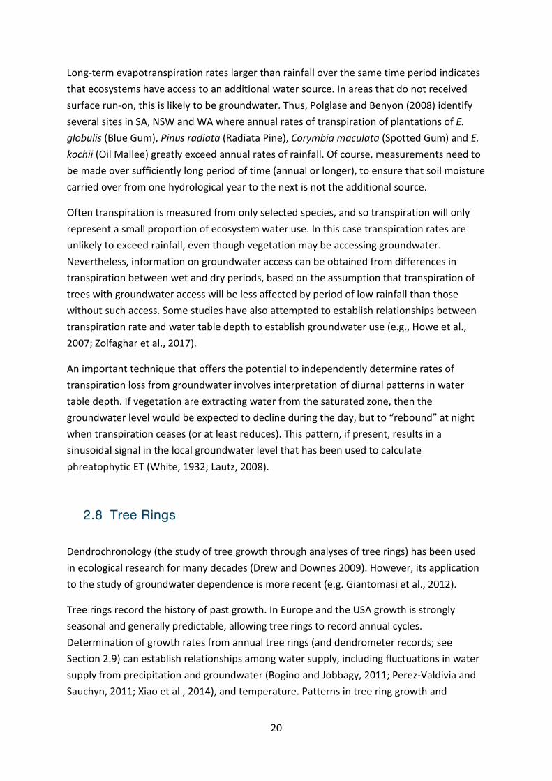
from depths of 8.3 m at least (the mulga did not grow at sites where groundwater was more shallow than this). Note that in Figure 21a, samples were taken at the end of the dry season (September) and wet season (April). In contrast, the water isotope composition of xylem water in E. camaldulensis and C. opaca were, in most trees sampled, close to and essentially indistinguishable from that of groundwater, for both sampling periods (Figure 21b).

Figure 21. Xylem sap and bore water stable isotope compositions sampled across multiple sites in the Ti Tree Basin in the wet and dry seasons. Trees were sampled within 50 m of bores. A number of sites were accessed so the data represent a range of groundwater depths. From Rumman et al. (2017).

4.5 Sapwood 13C and Leaf Vein Density

Figure 22 shows the foliar 13C discrimination values (Δ13C) as a function of groundwater depth for multiple sites sampled across the Ti Tree Basin for Mulga (Figure 22a, 22b) and E. camaldulensis and C. opaca (Figure 22c, 22d). It is clear that there is no relationship between Δ13C and depth to groundwater in the Mulga in either the wet or the dry season. In contrast, for E. camaldulensis and C. opaca, a stepwise regression model identified a break point in the relationship between Δ13C and depth to groundwater, in both sampling periods. In Figures 22c and 22d, breakpoints at 11.17 m (± 0.54 m) in September and 9.81 m (± 0.4 m) in April (ANOVA: 2, 38; F = 11.548; 2, 47; F = 14.67; P<0.01), were identified, and may represent the maximum depth from which significant groundwater is being extracted.

-100

-90

-80

-70

-60

-50

-40

-30

-20-8.5-7.5-6.5-5.5-4.5-3.5-2.5-1.5-0.5

δ2H

(‰)

δ18O (‰)

(a)BoreA.aneura (Sep-13, 8.3 m DTGW)A. aneura (Apr-14, 8.3 m DTGW)A. aneura (Sep-13, 20 m DTGW)A. aneura (Apr-14, 20 m DTGW)

-100

-90

-80

-70

-60

-50

-40

-30

-20-8.5-7.5-6.5-5.5-4.5-3.5-2.5-1.5-0.5

δ2H

(‰)

δ18O (‰)

(b)

BoreE. camaldulensis var. obtusa (Sep-13)E. camaldulensis var.obtusa (Apr-14)C. opaca (Sep-13)C. opaca (Apr-14)

45

Sep-2013 Apr-2014

(a)

DTGW (m)

0 10 20 30 40 50 60

∆13

C (‰

)

16

18

20

22

24

(b)

DTGW (m)

0 10 20 30 40 50 60

∆13

C (‰

)

16

18

20

22

24

Figure 22. Foliar 13C discrimination values (Δ13C) as a function of depth to groundwater (DTGW) for multiple sites sampled across the Ti Tree Basin. (a) and (b ) Mulga only; (c) and (d) E. camaldulensis and C. opaca. From Rumman et al. (2017).

Figure 23 demonstrates a similar methodological approach but using an independent measure of plant function, namely leaf vein density. Leaf vein density (LVD) is a functional trait influencing plant performance. The rate of maximum transpiration per unit leaf area is matched by the capacity of xylem to deliver water sufficient to accommodate this maximum (Brodribb and Holbrook, 2007; Sperry, 2000). Because of this, positive correlations between leaf-hydraulic conductance (Kleaf) and LVD, are observed (Brodribb et al., 2007; Sack and Holbrook, 2006). Because transpiration is directly linked to availability of water to roots, LVD should be influenced by depth-to-groundwater in deep rooted / groundwater accessing species. However, this correlation should be absent in species with shallow roots or which cannot access groundwater.

15

17

19

21

23

25

0 10 20 30 40 50 60

Δ13C

(%0)

DTGW

(c)

15

17

19

21

23

25

0 20 40 60

Δ13C

(%0)

DTGW

(d)

46

DTGW (m)

0 10 20 30 40 50 60

LVD

(mm

/mm

2 )

2

3

4

5

6

7

8

9

(a)

Figure 23. Leaf vein density (LVD) as a function of depth to groundwater (DTGW) across multiple sites sampled across the Ti Tree Basin. (a) A. aptaneura; (b) C. opaca and E. camaldulensis. From Rumman et al. (2017).

Figure 23a demonstrates that for A. aptaneura there was no correlation between LVD and DTGW, indicating that A. aptaneura does not access groundwater. This supports the results of the examination of foliar Δ13C (Figure 22a). In contrast, stepwise linear regression of data in Figure 23b identified a break point of 9.36 ± 0.6 m (ANOVA: 3, 59; F = 6.38; P<0.05) which agrees reasonably well with the two previous estimates (Figure 22).

A key development by Rumman et al. (2017) is their use of Δ13C to provide estimates of the upper and lower limit to groundwater use by the two species that were identified as using groundwater (E. camaldulensis and C. opaca). By combining three Australian data sets of foliar Δ13C (Miller et al., 2001; Stewart et al., 1995; Taylor 2008) plus the continental-scale determination of foliar Δ13C by Rumman, they demonstrated that the mean foliar Δ13C for E. camaldulensis and C. opaca did not conform to the regressions of the four independent data sets relating Δ13C to rainfall (Figure 24). Clearly E. camaldulensis in the Ti Tree is functioning as though it is receiving about 1700 mm of rainfall, despite only receiving a long-term average of 320 mm annual rainfall. Assuming no contribution of rainfall to transpiration by E. camaldulensis, 1700 mm represents the upper limit to groundwater use. Similarly an upper limit to annual groundwater use for C.opaca is estimated to be 837 mm (Figure 24). The lower limit to GW use is the difference between these values and rainfall, assuming all rainfall is used by these two species. Thus the lower limit to groundwater use is about 1400 mm for E. camaldulensis. Interestingly, O’Grady et al., (2009) showed that annual water use of riparian E. camaldulensis in the Ti-Tree was approximately 1642.5 m3 m-2 sapwood y-1. This yields an annual water use of 1568 mm y-1, encouragingly close to the estimate derived from Figure 24. O’Grady et al. (2009) estimate for annual water use for C. opaca to be 837 mm, in reasonable

2

3

4

5

6

7

8

9

10

0 10 20 30 40 50 60

LVD

(mm

/mm

2 )

DTGW (m)

47

agreement with the estimate from the average Δ13C of C. opaca and the regression in Figure 23 (ca 900 mm). Because groundwater for C.opaca is deeper (ca 8 -10 m) than that for E. camaldulensis (ca 1 - 3 m) a smaller rate of groundwater uptake for C.opaca is to be expected because xylem resistance to flow is presumably larger for the larger depth-to-groundwater for this species.

Figure 24. Relationships of discrimination against carbon-13 (Δ13C) with annual rainfall observed in different studies across Australia. The diamonds represent observations made in eastern Australia, northern Australia and New South Wales (Stewart et al., 1995; Miller et al., 2001; Taylor, 2008). The red squares are data from a continental-scale assessment of foliar Δ13C (Rumman, 2017). The black circle is the mean Δ13C of E. camaldulensis and the black square is the mean Δ13C of C. opaca, both sampled in the Ti Tree Basin.

y = 0.0024x + 18.103R² = 0.765

1516171819202122232425

0 500 1000 1500 2000 2500

Δ13 C

(%

o)

Annual rainfall (mm)

48

5. OTHER ARID ZONE STUDIES

5.1 Rocky Hill

Rocky Hill, approximately 25 km south east of Alice Springs, is located in the western part of the Amadeus Basin. The area contains groundwater of good quality, and has been designated as a future water supply for Alice Springs. There have been a number of investigations into the groundwater resources of the area (Read and Paul, 2000, 2002), as well as preliminary studies into the potential groundwater dependence of vegetation in the area (Cook et al., 2008).

The area is characterised by undulating plains of aeolian-derived quartz sand, underlain by shallow calcareous soils and sandy clay loams. The vegetation of the site is classified as being an Acacia low open woodland (Wilson et al., 1990) dominated by A. aptaneura, Acacia kempeana and Acacia estrophiolata. Groundwater salinity varies from less than 500 mg/L to more than 50 000 mg/L.

Deep soil water profiles were obtained at three sites beneath open woodland. At one site (18334) the water table is at approximately 23.4 m, while at the other two sites the water table is at approximately 51 m depth. Soil water potentials for the three sites are shown in Figure 25. In all cases, the observed water potential gradients would cause upward water movement throughout the profiles. Water potentials in 18334 are less than -9 MPa above 6 m depth, but increase with depth, but still above -2 MPa above 19 m. In 19379, matric potential is less than -4 MPa above 10 m, and less than -2 MPa above 11 m, while in 19187, matric potential is less than -4 MPa only above 4 m, and less than -2 MPa above 5 m. Variation between the profiles likely reflects variation within the landscape, including perhaps proximity of core sites to individual trees.

Leaf water potentials were only measured in the vicinity of 18334 (Figure 26). The maximum predawn leaf water potential measured in any of the species at this site was –1.3 MPa measured on E. camaldulensis – all other species have predawn leaf water potentials less than –1.9 MPa. The low water potential of E. camaldulensis suggests water extraction from approximately 20 m depth at this site. Leaf water potentials of most other species suggest water extraction from between 5 and 15 m depth.

49

Figure 25. Soil matric and water potential profiles obtained at Rocky Hill, south of Alice Springs. 18334 was drilled in May 2007, and 19379 and 19187 were drilled in July-August 2017. The water table is at 23.4 m in 18334 and at approximately 51 m at other two sites. All samples were collected by coring. After Howe et al. (2007) and Cook and White (2017).

Figure 26 also compares 18O composition of soil water with 18O composition of twig water. The 18O profile, which shows increasing enrichment towards the soil surface, is consistent with upwards water movement from the water table.

There is a relatively wide range of 18O composition of xylem water on individual species, although the lowest measured values (on A. victoriae) are also consistent with extraction from depths up to 20 m. Xylem water 18O composition of most other species suggest water extraction from between 5 and 15 m depth, although the 18O composition of A. aptaneura is significantly more enriched than in other species, and suggests that this water may have been sourced from the upper 2 m of the soil profile.

50

Figure 26. Soil water potentials and 18O values of soil water at Rocky Hill (RN018334), and comparison with leaf water potentials and 18O composition of twig water. Squares indicate total potential and 18O value of soil water, while pre-dawn and midday leaf water potentials are indicated by open and closed circles, respectively. The range of 18O values measured on twig samples for each species is indicated by a horizontal, with the mean value indicated by an open circle. After Cook et al. (2008). (The sample from 6 m depth that is shown in the original report has been deleted from this plot due to suspected contamination with drilling fluids.)

5.2 Pilbara, WA

The response of E. victrix to changes in groundwater level has also been monitored in the Pilbara region of Western Australia, where declines and rises in groundwater levels are associated with mine dewatering and disposal of dewatering water, respectively (Pfautsch et al., 2014). Mean annual precipitation in the Pilbara is similar to central Australia (mean of 315 mm at Newman), although rainfall events in the Pilbara are probably larger and more intense. Foliage density and water use were measured in E. victrix at four sites: two control sites were groundwater depth had been relatively constant at 6 and 29 m; a site where groundwater depth declined from approximately 8 to 19 m over a 3 year period between 2007 and 2010, and a site where groundwater rose from approximately 16 to 7 m over the same period.

51

Figure 27. Diel profiles of sapwood-related sap flow (QS) in Eucalyptus victrix. Data were averaged for Sep 2010 (solid line), Oct 2010 (dotted line), and Nov 2010 (dash-dotted line) across 5 trees per site. From Pfautsch et al. (2014).

Over the 4 year study period, foliage density varied within relatively small ranges, and did not reflect depth or access to groundwater. Trees at sites where groundwater was deep (Control29 and Drawdown; Figure 27) used less water compared with trees at sites where groundwater was shallower. The authors noted that it was unclear whether or not trees were able to access the groundwater at 29 m depth. However, much higher rates of water use of trees growing with water tables at 6 and 7 m, strongly suggests that trees have access to groundwater at these shallower depths. Where groundwater had risen from 16 to 7 m, water use was higher than at the control site where groundwater had remained at 6 m depth. This might suggest that the original water table depth of 16 m at the former site had led to increased root development, and so trees were able to access greater amounts of groundwater when the water table rose.

52

6. OTHER AUSTRALIAN AND INTERNATIONAL STUDIES

6.1 Global Rooting Depth Studies

Globally there have been two meta-analyses of maximum root depth (Canadell et al., 1996; Schenck and Jackson et al., 2002). Canadell et al., (1996) analysed literature that reported on 290 studies, covering 253 woody and herbaceous species. Within each of 11 biomes, ranging from Tundra and Boreal forest, to temperate deciduous forests and grasslands to tropical evergreen forests and savannas, the range in observed root depths within a single biome is very large, varying by factors of 5 – 10 in most cases, up to a factor of 10+ in others. Perhaps the most useful conclusion from Canadell et al., (1996) is that trees have deeper roots on average, than shrubs and crops, and that rooting depths in excess of 20 m have been measured in a number of different ecosystems.

Schenk and Jackson (2002) report on 475 profiles across 209 locations around the world. A major problem with the literature on root depths is that few field studies sample sufficiently deep to demonstrate maximum rooting depths. The majority of studies are confined to measurements within the top 1 m, occasionally 2 m, rarely beyond 2 m. Schenk and Jackson (2002) overcame this limitation by using root distribution functions to estimate maximum rooting depths.

Figure 28. Maximum rooting depth recorded in the literature for a range of ecosystems. From Canadell et al. (1996).

53

In this study, annual potential evapotranspiration (PET) and annual rainfall accounted for the largest proportion of variation in rooting depth, but still only accounted for about 15 % of variation globally (but up to almost 40 % is some ecosystems). At a global scale, annual PET, rainfall and length of the warm season were positively (but often weakly and non-linearly) correlated with rooting depths. Although maximum rooting depth increased with decreasing latitude between 80o and 30o, within the tropics there was no clear trend (but see below). A key finding was that within a climate zone (e.g., tropical, boreal), root depth was largest in water limited biomes. Schenk and Jackson (2005) also show that the probability of deep rooting increases with increased rainfall with arid and semi-arid biomes. Furthermore, rooting depths were deeper in sandy soils than clayey soils. Figure 29 shows the average extrapolated and non-extrapolated rooting depth for different biomes globally. It is clear that such analyses do not provide reliable nor sufficient information (see review of Australian studies in Section 6.2 below) that can be used to inform policy in central Australia.

Figure 29. Mean extrapolated and non-extrapolated rooting depths for global vegetation types. Extrapolated profiles are by definition deeper than non-extrapolated profiles. The extrapolations attempt to address the problem that many researchers sampled more shallowly than the entire root profile. Error bars represent 95% confidence intervals for means, based on sample sizes and estimates of interpolation and extrapolation errors.

54

Schenk and Jackson (2005) used soil texture data, monthly rainfall and potential evapotranspiration (PET) to model the global distribution of “deep” roots (defined as the presence of > 5% of all roots at depths larger than 2 m). They showed that deep roots were most likely to occur in seasonally dry, semi-arid to humid tropical regions under savanna or thorn-scrub vegetation or under seasonally dry evergreen forests. Coarse textured and fine textured soils also favoured deep roots (medium texture soils had a lower probability of containing deep rooted vegetation).

There are remarkably few direct, field-based examinations of root depth in Australia. The following table (Table 2) summarises some Australian, field-based studies. The only useful conclusion from field measurements of root depth is that there have not been any studies that have actually established a maximum root depth for any species in Australia. Observations of roots to 12 m (E. globulus; Doody and Benyon 2002) and 40 m (Eucalyptus marginata; Dell et al. 1983) have been made but to go beyond these we must use inferential methods to deduce root depths.

It is possible to infer rooting depth from knowledge of soil water potential as a function of depth, plus predawn canopy water potentials; or from knowledge of isotope composition as a function of depth, plus xylem water isotope composition. Thus, for example, O'Grady et al. (2006b) found that Corymbia clarksoniana in Queensland appeared to be accessing groundwater at depths of 7 – 10 m from application of these two methods. Additional examples of using stable isotope signatures through the soil profile, plus xylem water signatures, include Thorburn and Ehleringer (1995), Dawson (1996), Zencich et al. (2002), O'Grady et al. (2006b) and Costelloe et al. (2008). Zencich (2003) examined the use of various sources of water using 2H ratios in twigs of Banksia attenuata in Western Australia. They found that groundwater uptake during the dry season was to some extent determined by depth. Generally, where groundwater depth was less than 10 m, Banksia species had access to groundwater (see references cited in Groom 2004). Similarly, Howe et al. (2007) established that total tree water use in Corymbia opaca trees growing in the Ti Tree across a gradient of depth was slightly lower at sites with deeper groundwater than at sites with shallow water tables. Finally, groundwater depth is one determinant of the rate of growth and productivity of several important commercial species in SE Australia, including Pinus radiata, Eucalyptus globulus, E. grandis and Corymbia maculata (Benyon et al. 2006). In the Benyon et al. (2006) review, there was no apparent groundwater use at six sites where groundwater depth exceeded 7.5 m, whereas significant groundwater use occurred at 11 out of 14 sites where groundwater was shallower than 6 m.

55

Table 2. Some field observations of root depth in Australia.

Species/location Root depth Notes Reference

E. globulis ; SW Australia, 500 km SE of Perth

Sampling to 6 m via soil corer, followed by excavation to 6 m

Four sampling strategies simulated: coring only; bulk estimation plus coring; excavation by root diameter limit plus coring; root ball excavation plus coring

Sochacki et al. (2017)

Banksia spp. Whiteman Park, 20 km NE of Perth

GW depth varied between 3 – 3.7 m and root depth followed the capillary fringe

Examined seasonal redistribution of roots in response to variation in GW depth

Canham et al., 2012

Angophora bakeri, E. sclerophylla, Cumberland plains woodland, 55 km NW of Sydney NSW

Extensive rooting observed to 1.5 m depth

Trenching to 1.5 m depth Macinnis-Ng et al. (2010)

Tasmania, E. globulus

Maximum sampling depth (coring) was 1 m. Roots present at 1 m.

Very young (14 month) plantation O'Grady et al. (2005)

Eucalyptus marginate, SW Australia

Roots at depths of 14 m at several sites and 40 m at one site.

Sampling through coring and excavation

Dell et al. (1983)

E. marginata, SW Australia

5 – 12 m Stable isotopes used to determine depth of root water uptake

Farrington et al. (1996)

56

6.2 Groundwater Use by Vegetation

There is an extensive literature demonstrating that when groundwater is shallow (typically < 10 m), annual rates of vegetation water use can exceed annual rainfall. O’Grady et al. (2010, 2011) provide several summary tables of rates of groundwater discharge through vegetation from multiple sites in Australia, including the Chowilla floodplain, the Gnangara Mound in WA, the wheat belt of WA, the Green Triangle of south eastern SA, tropical coastal northern Queensland and the Riverina of NSW and Victoria. These tables are presented in Appendix 4. Table 3 provides additional examples where vegetation water use exceeds rainfall or where the proportion of groundwater use was calculated to be non-zero. Several key points are noteworthy from Tables 3 and Appendix 4:

1. A relatively new model by Cook and O’Grady (2006) demonstrated a range of proportions of GW use (from < 15 % to 100 %) across 4 tree species in northern Qld. This model is an improvement on previous end-member analyses of isotopic ratios of soil and xylem water.

2. Annual rates of water use by a wide range of species across a large range of sites within Australia are significantly larger than that of annual rainfall, indicating groundwater use.

3. Rates of daily groundwater use by vegetation range from ca 1 to 733 mm y-1 across a range of sites within Australia (Appendix 4 and Table 3).

4. The average groundwater use of 5 blue gum plots in the Green Triangle region of SA was 35 % of total annual tree water use (Benyon and Doody, 2004). One plot acquired all of its transpired water from the water table.

5. The mean annual transpiration rates for blue gum and radiata pine sites (mean of 8 sites) accessing groundwater in the Green Triangle was 789 mm y-1 but for similar sites (7 sites) not accessing groundwater, mean transpiration rates were 379 mm y-1 (Benyon and Doody, 2004). Six meters was the limit from which groundwater was extracted in these young (4 – 10 y old) plantations. Doody and Benyon (2002) did find groundwater extraction at 12 m in one unusual case where root access to groundwater was facilitated by fractures and a cave located above the groundwater.

57

Table 3. Some recent studies of rates of vegetation water use in relation to groundwater availability

Species/ Ecosystem Location Rates of vegetation water

use

Notes Reference

Corymbia clarksoniana, Lophostemon suaveolens, Eucalpytus platyphylla, Melaleuca viridiflora

Pioneer Valley, central Qld coast (sub-tropical)

5.72 l d-1( L. suaveolens) to 74.28 l d-1 (Eucalyptus platyphylla)

Sampling in late August. At the time of sampling, the proportion of groundwater extracted by the trees ranged from 100% for C. clarksoniana to <15% for L. suaveolens and E. platyphylla.

Cook and O’Grady (2006)

Eucalyptus kochii ssp. Borealis

Calecono Springs, 300 km of Perth, WA

1230 mm y-1 over shallow GW, 320 mm y-1 over deep GW; exceeds annual rainfall

Annual rainfall during the study period was 280 mm y-1 (longer term mean was 320 mm y-1)

Carter and White (2009)

E. globulus, Pinus radiata, Corymbia maculate, E. kochii

SA, WA, and NSW

GW > 6 m: Annual tree water use was 100 % of rainfall GW < 6 m: Annual tree water use was 157 %, 168 % or 486 % of rainfall

Annual rates of plantation tree water use exceed rainfall when GW is shallow

Polglase and Benyon (2008)

E. radiate, E. globoidea, E piperita, E.sieberi, E schlerophylla; dry sclerophyll forest

Kangaloon, 110 km SW Sydney, NSW

See Figure 30. Peak transpiration observed at approximately 4 m DGW and Emax declined with increasing DGW

Zolfaghar et al. (2017)

58

A detailed analyses of rates of tree water use as a function of depth-to-groundwater was conducted in the Kangaloon borefield in NSW (Zolfaghar et al., 2017). In this study, maximum rates of transpiration were observed at the second shallowest site (4.3 m) rather than at the shallowest site (2.4 m; Figure 30), a result ascribed to root anoxia occurring at the shallowest site. Such an effect has been observed previously.

Figure 30. Monthly average stand transpiration rate across 16 months across 4 depths-to-groundwater in the Kangaloon borefield, NSW, Australia. From Zolfaghar et al. (2017).

6.3 Limiting Depths for Vegetation Access of Groundwater

In a detailed study of leaf, wood, branch, tree and ecosystem traits in the Kangaloon borefield sites of NSW (e.g., specific leaf area, wood density, tree height), Zolfaghar (2014) established consistent trends in a number of traits as a function of groundwater depth (Figure 31). Mechanistic links between trait changes were apparent. Increased groundwater depth was associated with declines in basal area, tree height and leaf area index of native woodlands. A key aspect of this research was to develop an ecosystem-scale response function for groundwater depth, and to examine whether a threshold in groundwater depth is apparent. Zolfaghar thus developed a composite index of 18 vegetation traits, each trait normalised with reference to the largest value recorded across all species and sites. The composite of these normalised values

59

provides a measure of ecosystem condition, is plotted versus groundwater depth in Figure 31 (Eamus et al., 2015).

Figure 31. The normalised response curve for average normalised values of 18 leaf, wood, branch, tree and ecosystem traits, plotted as a function of depth-to-groundwater. From Eamus et al. (2015), after Zolfaghar (2014).

Figure 31 clearly demonstrates a threshold in groundwater depth, at around 8 - 9 m, below which trait values clearly show a significant decline, and above which values are maximal. This is the first trait-based demonstration of a threshold value for groundwater depth, beyond which significant changes in ecophysiological and ecological trait values occurs. What this relationship doesn’t say, is that it is safe to pump groundwater from depths less than 1 m, to depths of < 9 m, before changes in ecophysiology and ecology occur because the depth-to groundwater gradient sampled was a naturally occurring gradient and species and individuals have been established at each site for centuries (species) or decades (individual trees). Consequently we do not know whether changing the natural groundwater depth regime at any site with depths less than 10 m will induce significant changes in ecophysiology or ecology. Only an experimentally induced change in depth that is maintained for many years will offer insight to the changes that may occur in response.

The estimated 9 m threshold value is consistent with other studies. For example, two recent reviews based on water balance approaches concluded that groundwater uptake ceased when depths exceeded 7.5 m (Benyon et al., 2006) or 8–10 m (O’Grady et al., 2010; Figure 32). Kath et al. (2014) identified thresholds of groundwater depth of between 12.1 and 26.6

60

m across 118 sites in south-eastern Australia (within the Murray-Darling Basin) for two tree species. Thus the existence of a threshold appears reasonable – but it appears to be site and species specific. The work of Rumman and others discussed in Section 4.5 demonstrated a threshold of about 10 m for tree species in the Ti Tree, consistent with that of Zolfaghar et al. (2017) in NSW.

Most of the above studies have examined the relationship between ecosystem condition and groundwater depth in stable systems. Where groundwater levels decline through groundwater extraction, the relationship between ecosystem condition and groundwater depth becomes more complex and there are no published experimental data available for Australian species where the impact of different rates of increase in depth-to-groundwater have been examined..

Figure 32. The influence of water table depth on groundwater uptake for groundwater discharge studies in Australia. From O’Grady et al. (2010).

61

7. CONCLUSIONS

Investigations in open woodland ecosystems in the Ti Tree Basin show the use of regional groundwater by overstory trees (particularly C. opaca) where water table depths are at 8 - 12 m, and in some cases up to 20 m. In particular:

1) Soil water potential data suggests that a significant number of tree roots extend to at least 8 m depth, with some evidence for tree roots to 15 m and more.

2) Water isotope data (18O) provides supporting evidence for extraction of soil water from at least 8 m depth by C. opaca.

3) Sapflow data shows that total water use of C. opaca is much greater where water tables are 12 m and less, than in areas with water tables 20 m or more. The large difference in transpiration rate suggests that there would be a significant change in tree condition if water tables are lowered from 12 to 20 m.

4) Foliar 13C and leaf vein density show significant differences between areas with water tables less than and greater than 10 m depth.

In areas with water tables of 6 m or less, more shallow-rooted species are able to access groundwater, including E. victrix. Stirling Swamp is also a GDE, with total annual transpiration of the ecosystem greatly exceeding annual rainfall. E. camaldulensis also access groundwater, and tend to occur in riparian areas and where perched shallow aquifers are present. Although there is some evidence from soil water potential data that some open woodland vegetation (most likely C. opaca) can extend roots to beyond 15 m, this is based only on a single profile of soil water potential, and these data can sometimes be affected by drying of the soil during sample collection.

These results are supported by arid zone GDE studies at Rocky Hill, where soil water potential profiles show root extraction of soil water to at least 10 m in places, with some evidence of extraction to 20 m; and in the Pilbara, E. victrix has been shown to use groundwater at 6 – 7 m depth.

Investigations at other sites have found significant differences in transpiration of woodland ecosystems and also measurable differences in ecosystem structure and function where water table depths are in excess of 10 m, compared to areas with shallower water tables.

62

REFERENCES

Adams HD, Kolb TE (2005) Tree growth response to drought and temperature in a mountain landscape in northern Arizona, USA. J. Biogeog., 32, 1629-1640. doi:10.1111/j.1365-2699.2005.01292.x.

Akasheh OZ, Neale CMU, Jayanthi H (2008) Detailed mapping of riparian vegetation in the middle Rio Grande River using high resolution multi-spectral airborne remote sensing. J. Arid Environ., 72, 1734–1744.

Atkinson D, Dawson LA (2000) Root growth: methods of measurement. In: Smith KA, Mullins CE (eds), Soil and Environmental Analysis: Physical Methods. Marcel Dekker, New York, 637p.

Baldocchi DD, Ryu Y (2011) A synthesis of forest evaporation fluxes – from days to years – as measured with eddy covariance. In: Levia DF, Carlyle-Moses D, Tanaka T (eds), Forest Hydrology and Biogeochemistry: Synthesis of Past Research and Future Directions. Springer Sciences Business Media B. V., Dordrecht, The Netherlands, 101–116.

Benyon RG, Doody TM (2004) Water Use by Tree Plantations in South East South Australia. CSIRO Forestry and Forest Products, Mt Gambier.

Benyon RG, Theiveyanathan S, Doody TM (2006) Impacts of tree plantations on groundwater in south-eastern Australia. Aust. J. Bot., 54, 181–192.

Bithell SL, Tran-Nguyen LTT, Hearnden MN, Hartley DM (2014) DNA analysis of soil extracts can be used to investigate fine root depth distribution of trees. AoB PLANTS, 7, plu091. doi:10.1093/aobpla/plu091

Bogino SM, Jobbagy EG (2011) Climate and groundwater effects on the establishment, growth and death of Prosopis caldenia trees in the Pampas (Argentina). For. Ecol. Manag., 262, 1766-1774. doi:10.1016/j.foreco.2011.07.032.

Brodribb TJ, Feild TS, Jordan GJ (2007) Leaf maximum photosynthetic rate and venation are linked by hydraulics, Pl. Phys., 144(4), 1890-1898.

Canadell J Jackson RB, Ehleringer JR, Mooney HA,Sala OE, Schulze ED (1996) Maximum rooting depth of vegetation types at the global scale. Oecologia, 108, 583-595.

Canham CA, Froend RH, Stock WD, Davies M (2012) Dynamics of phreatophyte root growth relative to a seasonally fluctuating water table in a Mediterranean-type environment. Oecologia, 170, 909 -916.

Carter JL, White DA (2009) Plasticity in the Huber value contributes to homeostasis in leaf water relations of a mallee Eucalypt with variation to groundwater depth. Tree Physiology, 29(11), 1407-18.

Chimner RA, Cooper DJ (2004) Using stable oxygen isotopes to quantify the water source used for transpiration by native shrubs in the San Luis Valley, Colorado USA. Plant and Soil, 260, 225 - 236.

63

Cleverly J, Eamus D, Gorsel E van, Chen C, Rumman R, Luo Q, Restrepo-Coupe N, Li L, Kljun N, Faux R, Yu Q, Huete A (2016) Productivity and evapotranspiration of two contrasting semiarid ecosystems following the 2011 global carbon land sink anomaly. Agriculture and Forest Meteorology, 220, 151c – 159.

Clifton R, Evans C (2001) Environmental water requirements of groundwater dependent ecosystems. Environmental Flows Initiative Technical Report no. 2. Commonwealth of Australia, Canberra.

Clifton C, Cossens B, McAuley C, Evans R, Cook P, Howe P, Boulton A (2009) A framework for assessing the environmental water requirements of groundwater dependent ecosystems. Report 1: Assessment toolbox. Land and Water Australia.

Cocozza C, Giovannelli A, Traversi ML, Castro G, Cherubini P, Tognetti R (2011) Do tree-ring traits reflect different water deficit responses in young poplar clones (Populus x canadensis Monch 'I-214' and P. deltoides 'Dvina')? Trees-Structure and Function, 25, 975-985. doi: 10.1007/s00468-011-0572-8.

Conejero W, Alarcón JJ, García-Orellana Y, Abrisqueta JM, Torrecillas A (2007) Daily sapflow and maximum daily trunk shrinkage measurements for diagnosing water stress in early maturing peach trees during the post harvest period. Tree Physiol., 27, 81–88.

Contreras S, Jobbagy EG, Villagra PE, Nosetto MD, Puigdefabregas J (2011) Remote sensing estimates of supplementary water consumption by arid ecosystems of central Argentina. J. Hydrol., 397, 10–22.

Cook PG, O’Grady AP, Wischusen JDH, Duguid A, Fass T, Eamus D (2008) Ecohydrology of sand plain woodlands in central Australia. Report to Natural Heritage Trust (Project number 2005/147).

Cook PG, O’Grady AP (2006) Determining soil and ground water use of vegetation from heat pulse, water potential and stable isotope data. Oecologia, 148, 97-107.

Cook PG, Walker GR (1989) Groundwater Recharge in South Western New South Wales. Centre for Research in Groundwater Processes. Report No. 9.

Costelloe JF, Payne E, Woodrow IE, Irvine EC, Western AW, Leaney FW (2008) Water sources accessed by arid zone riparian trees in highly saline environments, Australia. Oecologia, 156, 43-52.

Dawson TE, Ehleringer JR (1991) Streamside trees that do not use stream water. Nature, 350, 335-337.

Dawson TE, Pate JS (1996) Seasonal water uptake and movement in root systems of Australian phreatophytic plants of dimorphic root morphology: a stable isotope investigation. Oecologia, 107, 12-20.

Dell B, Bartle J, Tacey W (1983) Root occupation and root channels of Jarrah forest subsoils. Australian Journal of Botany, 31, 615-627.

64

Doody TM, Benyon RG, Theiveyanathan S, Koul V, Stewart L (2014) Development of pan coefficients for estimating evapotranspiration from riparian woody vegetation. Hydrol. Process., 28, 2129–2149. doi:10.1002/hyp.9753.

Drake PL, Coleman BF, Vogwill R (2013) The response of semi-arid ephemeral wetland plants to flooding: linking water use to hydrological processes. Ecohydrology, 6, 852-862.

Drake PL, Franks PJ (2003) Water resource partitioning, stem xylem hydraulic properties, and plant water use strategies in a seasonally dry riparian tropical rainforest. Oecologia, 137, 321-329. doi:10.1007/s00442-003-1352-y.

Dresel PE, Clark R, Cheng X, Reid M, Terry A, Fawcett J, Cochrane D (2010) Mapping Terrestrial GDEs: Method development and example output. Victoria Department of Primary Industries, Melbourne, 66pp.

Drew DM, Downes GM (2009) The use of precision dendrometers in research on daily stem size and wood property variation: A review. Dendrochronologia, 27, 169-172.

Drew DM, O’Grady AP, Downes GM, Read J, Worledge D (2008) Daily patterns of stem size variation in irrigated and unirrigated Eucalyptus globulus. Tree Physiol., 28, 1573-1581.

Eamus D, Froend R, Loomes R, Hose G, Murray B (2006) A functional methodology for determining the groundwater regime needed to maintain the health of groundwater dependent vegetation. Australian Journal of Botany, 54, 97-114.

Everitt JH, DeLoach CJ (1990) Remote sensing of Chinese Tamarisk (Tamarix chinensis) and associated vegetation. Weed Science, 38, 273–278.

Farrington P, Turner JV, Gailitis V (1996) Tracing water uptake by Jarrah (E. marginata) trees using natural abundance of deuterium. Trees, 11, 9-15.

Fawcett RG, Collis-George N (1967) A filter paper method for determining the moisture characteristic of soil. Aust. J. Exp. Agric. Anim. Husb., 7, 162-167.

February EC, Higgins SI, Newton R, West AG (2007) Tree distribution on a steep environmental gradient in an arid savanna. J. Biogeog., 34, 270-278.

Galindo A, Rodrigues P, Mellisho CD, Torrecillas E, Moriana A, Cruz ZN, Conejero W, Moreno F, Terrecillas A (2013) Assessment of discreetly measured indicators and maximum daily trunk shrinkage for detecting water stress in pomegranate trees. Ag. For. Met., 180, 58-65.

Giantomasi MA, Roig-Juñent FA, Villagra PE (2012) Use of differential water sources by Prosopis flexuosa DC: a dendroecological study. Plant Ecol., 214(1), 11-27. doi:10.1007/s11258-012-0141-2.

Grant JC, Nichols JD, Yao RL, Smith RGB, Brennan PD, Vanclay JK (2012) Depth distribution of roots of Eucalyptus dunnii and Corymbia citriodora subsp. variegata in different soil conditions. Forest Ecology and Management, 269, 249-258.

65

Greacen EL, Walker GR, Cook PG (1987) Evaluation of the filter paper method for measuring soil water suction. Proc. Int. Conf. Meas. Soil and Plant Water Status, Utah State Univ., July 1987.

Groom PK (2004) Rooting depth and plant water relations explain species distribution patterns within a sandplain landscape. Functional Plant Biology, 31, 423-428.

Huete A, Didan K, Miura T, Rodriguez EP, Gao X, Ferreira LG (2002) Overview of the radiometric and biophysical performance of the MODIS vegetation indices. Remote Sens. Environ., 83, 195-213. doi:10.1016/s0034-4257(02)00096-2.

Hanson RT, Dettinger MD, Newhouse MW (2006) Relations between climatic variability and hydrologic time series from four alluvial basins across the southwestern United States. Hydrogeol. J., 14, 1122-1146. doi:10.1007/s10040-006-0067-7.

Harrington GA, Herczeg AL, Cook PG (1999) Groundwater sustainability and water quality in the Ti-Tree Basin, central Australia. CSIRO Land and Water, Tech. Rep. 53/99.

Harrington GA, Cook PG, Herczeg AL (2002) Spatial and temporal variability of ground water recharge in central Australia: a tracer approach. Ground Water, 40(5), 518-527.

Hatton, T., Evans, R., 1998. Dependence of ecosystems on groundwater and its significance to Australia. Occasional Paper No. 12/98, Land and Water Resources Research and Development Corporation, Canberra.

Howe P, O’Grady A, Cook P, Fass T (2007) A Framework for Assessing the Environmental Water Requirements of Groundwater Dependent Ecosystems. Report 2: Field Studies. Land and Water Australia.

Hultine KR, Bush SE, Ehleringer JR (2010) Ecophysiology of riparian cottonwood and willow before, during, and after two years of soil water removal. Ecol. Appl., 20, 347-361. doi:10.1890/09-0492.1.

Jeffrey SJ, Carter JO, Moodie KB, Beswick AR (2001) Using spatial interpolation to construct a comprehensive archive of Australian climate data. Environ. Model. Softw., 16, 309-330.

Jin XM, Schaepman ME, Clevers JG, Su ZB, Hu G (2011) Groundwater depth and vegetation in the Ejina area, China. Arid Land Res. Manage., 25, 194–199.

Kath J, Reardon-Smith K, Le Brocque AF, Dyer FJ, Dafny E, Fritz L, Batterham M (2014) Groundwater decline and tree change in floodplain landscapes: Identifying non-linear threshold responses in canopy condition. Global Ecology and Conservation, 2, 148-160.

Kray J, Cooper D, Sanderson J (2012) Groundwater use by native plants in response to changes in precipitation in an intermountain basin. J. Arid Environ., 83, 25-34.

Lageard JGA, Drew IB (2008) Hydrogeomorphic control on tree growth responses in the Elton area of the Cheshire Saltfield, UK. Geomorphology, 95, 158-171. doi:10.1016/j.geomorph.2007.05.017.

Lamont BB (2003) Structure, ecology and physiology of root clusters—a review. Plant Soil, 248, 1-19.

66

Lautz LK (2008) Estimating groundwater evapotranspiration rates using diurnal water-table fluctuations in a semi-arid riparian zone. Hydrogeol. J., 16, 483–497.

Le Maitre DC, Scott DF, Colvin C (1999) A review of information on interactions between vegetation and groundwater. Water SA, 25(2), 137-152.

Lorenzo H, Pérez-Gracia V, Novo A, Armesto J (2010) Forestry applications of ground-penetrating radar. Forest Systems, 19(1), 5-17.

Lv J, Wang XS, Zhou Y, Qian K, Wan L, Eamus D, Tao Z (2012) Groundwater-dependent distribution of vegetation in Hailiutu River catchment, a semi-arid region in China. Ecohydrology, 6, 142–149.

Macinnis-Ng CMO, Fuentes S, O'Grady AP, Palmer AR (2010) Root biomass distribution and soil properties of an open woodland on a duplex soil. Plant and Soil, 327, 377–388.

Máguas C, Rascher KG, Martins-Loução A, Carvalho P, Pinho P, Ramos M, Correia O, Werner C (2011) Responses of woody species to spatial and temporal ground water changes in coastal sand dune systems. Biogeosciences, 8, 3823–3832, doi:10.5194/bg-8-3823-2011.

McCarroll D, Loader NJ (2004) Stable isotopes in tree rings. Quaternary Sci. Rev., 23, 771-801. doi: 10.1016/j.quascirev.2003.06.017.

Miller JM, Williams RJ, Farquhar GD (2001) Carbon isotope discrimination by a sequence of Eucalyptus species along a subcontinental rainfall gradient in Australia. Functional Ecology, 15(2), 222-232.

Münch Z, Conrad J (2007) Remote sensing and GIS based determination of groundwater dependent ecosystems in the Western Cape, South Africa. Hydrogeol. J., 15, 19-28.

Nagler PL, Glenn E, Nguyen U, Scott R, Doody T (2013) Estimating riparian and agricultural actual evapotranspiration by reference evapotranspiration and MODIS enhanced vegetation index. Remote Sensing, 5, 3849–3871.

Naumburg E, Mata-Gonzalez R, Hunter RG, McLendon T, Martin DW (2005) Phreatophytic vegetation and groundwater fluctuations: a review of current research and application of ecosystem response modelling with an emphasis on great basin vegetation. Environ. Manag., 35, 726–740, doi:10.1007/s00267-004-0194-7.

Newman EIA (1966) Method of estimating the total length of root in a sample. Journal of Applied Ecology, 3(1), 139-145.

Nolan RH, Fairweather KA, Tarin T, Santini NS, Cleverly J, Faux R, Eamus D (2017) Divergence in plant water-use strategies in semiarid woody species. Functional Plant Biology, 44(11), 1134-1146. https://doi.org/10.1071/FP17079

Oberhuber W, Stumbock M, Kofler W (1998) Climate tree-growth relationships of Scots pine stands (Pinus sylvestris L.) exposed to soil dryness. Trees-Structure and Function, 13, 19-27.

O'Grady AP, Worledge D, Battaglia M (2005) Temporal and spatial changes in fine root distributions in a young Eucalyptus globulus stand in southern Tasmania. Forest Ecol. Manag., 214, 373-383.

67

O’Grady AP, Cook PG, Howe P, Werren G (2006) Groundwater use by dominant tree species in tropical remnant vegetation communities. A. J. Bot., 54, 155-171.

O’Grady AP, Cook PG, Eamus D, Duguid A, Wischusen JDH, Fass T, Worldege D (2009) Convergence of tree water use within an arid-zone woodland. Oecologia, 160, 643-655.

O’Grady A, Carter J, Holland K (2010) Review of Australian Groundwater Discharge Studies of Terrestrial Systems. Water for a Healthy Country Flagship Report series ISSN: 1835-095X.

O’Grady AP, Carter JL, Bruce J (2011) Can we predict groundwater discharge from terrestrial ecosystems using existing eco-hydrological concepts? Hydrology and Earth System Sciences, 15, 3731-3739.

Orellana F, Verema P, Loheide SP, Daly E (2012) Monitoring and modelling water-vegetation interactions in groundwater-dependent ecosystems. Reviews of Geophysics, 50, RG3003. doi:10.1029/2011RG000383.

Osmond CB, Austin MP, Berry JA, Billings WD, Boyer JS, Dacey JWH, Nobel PS, Smith SD, Winner WE (1987) Stress physiology and the distribution of plants. Bioscience, 37, 38-47.

Perez-Valdivia C, Sauchyn D (2011) Tree-ring reconstruction of groundwater levels in Alberta, Canada: Long term hydroclimatic variability. Dendrochronologia, 29, 41-47. doi:10.1016/j.dendro.2010.09.001.

Pfautsch S, Dodson W, Madden S, Adams MA (2014) Assessing the impact of large-scale water table modifications on riparian trees: a case study from Australia. Ecohydrology, 8(4), 642-651.

Phillips, D. L. and Gregg, J. W. 2003 Source partitioning using stable isotopes: coping with too many sources. Oecologia, 136, 261-269.

Polglase P, Benyon R (2008) The impacts of plantations and native forests on water security: Review and scientific assessment of regional issues and research needs. Forest and Wood Products Australia.

Potts DL, Williams DG (2004) Response of tree ring holocellulose delta C-13 to moisture availability in Populus fremontii at perennial and intermittent stream reaches. Western North American Naturalist, 64, 27-37.

Prior LD, Grierson PF, McCaw WL, Tng DYP, Nichols SC, Bowman D (2012) Variation in stem radial growth of the Australian conifer, Callitris columellaris, across the world's driest and least fertile vegetated continent. Trees-Structure and Function, 26, 1169-1179. doi:10.1007/s00468-012-0693-8.

Read RE, Paul RJ (2000) Rocky Hill – Ooraminna groundwater investigation 1998 & 1999. Northern Territory Department of Lands, Planning and Environment. Report No. 16/1998A (2 volumes).

Read RE, Paul RJ (2002) Rocky Hill – Ooraminna groundwater investigation 2000. Northern Territory Department of Infrastructure, Planning and Environment. Report No. 05/2000A.

68

Read R, Tickell SJ (2007) The Ti-tree Basin Aquifer, Hydrogeological Map, Northern Territory Government. Department of Natural Resources, Entertainment and the Arts.

Richardson S, Irvine E, Froend R, Boon P, Barber S, Bonneville B (2011) Australian groundwater-dependent ecosystems toolbox. Part 2: assessment tools. National Water Commission, Canberra.

Rumman R, Cleverly J, Nolan RH, Tarin T, Eamus D (2017) Speculations on the application of foliar 13C discrimination to reveal groundwater dependency of vegetation, provide estimates of root depth and rates of groundwater use. Hydrol. Earth Syst. Sci. Discuss., https://doi.org/10.5194/hess-2017-540.

Rood SB, Goater LA, Gill KM, Braatne JH (2011) Sand and sandbar willow: A feedback loop amplifies environmental sensitivity at the riparian interface. Oecologia, 165, 31-40.

Sack L, Holbrook, NM (2006) Leaf hydraulics. Ann. Rev. of Pl. Biol., 57, 361-381.

Sarris D, Christodoulakis D, Korner C (2007) Recent decline in precipitation and tree growth in the eastern Mediterranean. Glob. Chng. Biol., 13, 1187-1200. doi:10.1111/j.1365-2486.2007.01348.x.

Schenk HJ, Jackson RB (2002) The global biogeography of roots. Ecological Monographs, 72 (3), 311-328.

Schenka HJ, Jackson RB (2005) Mapping the global distribution of deep roots in relation to climate and soil characteristics. Geoderma, 126, 129-140.

Schenk HJ (2008) The shallowest possible water extraction profile: a null model for global root distributions. Vadose Zone Journal, 7, 1119-1124.

Scurlock D (1998) From the Rio to the Sierra: An Environmental History of the Middle Rio Grande Basin. General Technical Report RMRS-GTR-5, USDA Forest Service, Rocky Mountain Research Station, Fort Collins, CO.

Shanafield M, Cook PG, Gutierrez-Jurado HA, Cleverly J, Eamus D (2015) Field comparison of methods for estimating groundwater discharge by evaporation and evapotranspiration in an arid-zone playa. Journal of Hydrology, 527, 1073-1083.

Sochacki SJ, Ritson P, Brand B, Harper RJ, Bell B (2017) Accuracy of tree root biomass sampling methodologies for carbon mitigation projects. Ecological Engineering, 98, 264-274.

Stewart GR, Turnbull M, Schmidt S, Erskine P (1995) 13C natural abundance in plant communities along a rainfall gradient: a biological integrator of water availability. Functional Plant Biology, 22(1), 51-55.

Stock WD, Bourke L, Froend RH (2012) Dendroecological indicators of historical responses of pines to water and nutrient availability on a superficial aquifer in south-western Australia. For. Ecol. and Manag., 264, 108-114.

Taylor D (2008) Tree, leaf and branch trait coordination along an aridity gradient. PhD Thesis. University of Technology Sydney.

69

Thorburn PJ, Ehleringer JR (1995) Root water uptake of field-growing plants indicated by measurements of natural abundance deuterium. Plant and Soil, 177, 225-233.

Tooth S (1999) Floodouts in Central Australia. In: Miller AJ, Gupta A (eds) Varieties of Fluvial Form. Wiley, Chichester, p.219-247.

Tweed S O, LeBlanc M, Webb JA, Lubczynski MW (2007) Remote sensing and GIS for mapping groundwater recharge and discharge areas in salinity prone catchments, southeastern Australia. Hydrogeol. J., 15, 75-96.

Villeneuve S, Cook PG, Shanafield M, Wood C, White N (2015) Groundwater recharge via infiltration through an ephemeral riverbed, central Australia. Journal of Arid Environments, 117, 47-58.

Wang J, Bras R (2011) A model of evapotranspiration based on the theory of maximum entropy production. Water Resour. Res., 47(3), doi:10.1029/2010WR009392.

White WN (1932) A method of estimating ground-water supplies based on discharge by plants and evaporation from soil: Results of investigations in Escalante Valley, Utah, in: Interior, US Geological Survey, Washington, D.C., p. 105.

Wood C, Cook PG, Harrington GA, Knapton A (2017) Constraining spatial variability in recharge and discharge in an arid environment through modelling carbon-14 with improved boundary conditions. Water Resources Research, 53, 142-157.

Xiao SC, Xiao HL, Peng XM, Tian QY (2014) Intra-annual stem diameter growth of Tamarix ramosissima and association with hydroclimatic factors in the lower reaches of China's Heihe River. Journal of Arid Land, 6, 498-510. doi:10.1007/s40333-013-0248-x.

Zencich SJ, Froend RH, Turner JV, Gailitis V (2002) Influence of groundwater depth on the seasonal sources of water accessed by Banksia tree species on a shallow, sandy coastal aquifer. Oecologia, 131, 8-19.

Zeppel M (2013) Convergence of tree water use and hydraulic architecture in water-limited regions: a review and synthesis. Ecohydrology, 6, 889-900.

Zolfaghar S (2014) Comparative ecophysiology of Eucalyptus woodlands along a depth-to-groundwater gradient, PhD thesis, University of Technology, Sydney, 228p.

Zolfaghar S, Villalobos-Vega R, Cleverly J, Zeppel M, Rumman R, Eamus D (2014) The influence of depth-to-groundwater on structure and productivity of Eucalyptus woodlands. Australian Journal of Botany, 62, 428-437.

Zolfaghar S, Villalobos-Vega R, Zeppel M, Cleverly J, Rumman R, Hingee M, Boulain N, Li Z, Eamus D (2017) Transpiration of Eucalyptus woodlands across a natural gradient of depth-to-groundwater. Tree Physiology, 37, 961-975.

Zweifel R, Zimmermann L, Newbery DM (2005) Modelling tree water deficit from microclimate: an approach to quantifying drought stress. Tree Physiology, 25, 147-156.

70

71

APPENDIX 1. MEASUREMENT OF WATER POTENTIAL

1.1.1 Pressure bomb

The “Scholander” pressure chamber, or pressure bomb, measures the water potential of excised leaves or xylem of excised branches. A detailed description of the use of the pressure bomb is provided on pages 88 -90 in Eamus et al. (2006). The maximum pressure attainable in commercial pressure bombs is 10 MPa, and therefore the minimum water potential that can be measured is -10 MPa. It requires connection to a cylinder of compressed gas and has significant safety requirements in its correct use.

4.3.2 Thermocouples

Thermocouple psychrometers can be used to measure the water potential of soil, leaves and more recently, stems. The water potential of Intact leaves, or leaf discs, can be used with different models of psychrometer. These systems are small, but require significant equilibration times (tens of minutes), unlike the pressure bomb. The existence of temperature gradients between leaf and thermocouple introduce significant errors in the measurements but these can be corrected for.

Stem psychrometers can be attached to data loggers and allowed to run in the field without manual input, unlike leaf thermocouples. The following two photographs illustrate the installation of a stem psychrometer.

4.3.3 Cooled mirror dewpoint hygrometer

The WP4C cooled mirror hygrometer measures the dew point of air that has equilibrated to the water potential of a sample (soil, large leaf disc) sealed in a small chamber. The range of water potentials that can be measured is much larger than that of a pressure chamber or thermocouple psychrometer, from -0.1 to a notional -300 MPa. Equilibration times are a notional 5 – 10 mins, but can be longer for low values of water potential.

72

Figure A1.1. A stem psychrometer sold by ICT International, positioned on a cotton stem. This photo shows the psychrometer installed prior to installation of thermal insulation (see below). From: http://www.ictinternational.com/casestudies/logging-water-potential-of-cotton.

Figure A1.2. The integrated stand alone logger of the PSY1 attached to the cotton stem. The PSY1 supplies power from an internal battery, controls the Peltier cooling pulse, logging interval and data collection of the psychrometer. All data, both raw measurements and

73

processed water potentials is saved on an internal 2GB MicroSD memory card. From: http://www.ictinternational.com/casestudies/logging-water-potential-of-cotton.

Figure A1.3. A cooled mirror dewpoint hygrometer. From: https://www.decagon.com/en/soils/benchtop-instruments/wp4c-water-potential-meter/

74

APPENDIX 2. HYDRUS MODEL OF SOIL WATER FLOW

To investigate the influence of soil matric potential (induced by vegetation and surface

evaporative demand), water table depths, and soil types on plant water availability, a steady

state, homogenous 1 dimensional soil column was simulated using Hydrus 1D; a numerical

model widely used to simulate unsaturated zone processes (Simunek et al., 2005). The 1d

column represented the unsaturated zone, and so the bottom pressure boundary was set to

0 kPa (pressures at the water table). The upper boundary pressure was based on observed

soil matric potentials beneath native vegetation and was set as -4000 kPa. A number of

different soil types were simulated, the relevant van Genuchten parameters are shown in

Table A2.1. (Note that soil types containing sand did not reach steady state in the simulation

period and where therefore removed from the investigation.) Column lengths varied from 1

m (representing a very shallow water table) to 64 m (representing a deep water table),

column was discretised into 900 nodes (node spacing varied from 1 – 7 cm). Other than the

top and bottom nodes, the initial pressure distribution within the column was set to -40 kPa.

The model was run to steady state over a period of 100,000 years (min. time step of 2.7 x

10-6 years and max time step of 1000 years). Steady state conditions were determined based

on the flux profile within the column; a uniform flux with depth within the column indicated

steady state conditions had been reached. Values of the steady state flux were then

determined for each simulation. These represent the potential rate of groundwater

discharge created by root extraction at different depths above groundwater and for

different soil types.

Table A2.1. Van Genuchten parameters used in the simulations.

Type Qr

(cm3cm-3) Qs

(cm3cm-3) Α

(cm-1) n Ks

(cm/day) silt 0.034 0.46 0.016 1.37 2190

silt loam 0.067 0.45 0.02 1.41 3942 clay loam 0.095 0.41 0.019 1.31 2277.6

silty clay loam 0.089 0.43 0.01 1.23 613.2 silty clay 0.07 0.36 0.005 1.09 175.2

clay 0.068 0.38 0.008 1.09 1752

75

APPENDIX 3. TI TREE VEGETATION SURVEY

Table A3.1. Plant species recorded at the 10 study sites in the Ti Tree basin with information on status (native, exotic), growth form (tree, shrub, graminoid, forb), longevity (annual, perennial), distribution (number of sites) and mean abundance across the DGW gradient.

Species Status Growth form Longevity Distribution Abundance (per 103 m2)

Abutilon otocarpum Native Shrub Perennial 2 0.4 Acacia aptaneura Native Shrub Perennial 3 3.9 Acacia apteneura Native Shrub Perennial 2 2.4 Acacia kempeana Native Shrub Perennial 1 0.6 Acacia melleodora Native Shrub Perennial 1 0.1 Acacia sericophylla Native Shrub Perennial 1 0.7 Acacia tetragonophylla Native Shrub Perennial 1 0.1 Acacia victoriae Native Shrub Perennial 1 0.7 Androcalva loxophylla Native Shrub Perennial 2 3.0 Aristida holathera Native Graminoid Annual 10 7.3 Aristida inaequiglumis Native Graminoid Perennial 1 0.6 Boerhavia coccinea Native Forb Perennial 1 0.3 Cenchrus ciliaris Exotic Graminoid Perennial 1 4.5 Cenchrus setiger Exotic Graminoid Perennial 2 4.7 Cleome viscosa Native Forb Annual 2 2.4 Dactyloctenium radulans Native Graminoid Annual 2 0.5 Enneapogon polyphyllus Native Graminoid Annual 3 0.6 Eragrostis eriopoda Native Graminoid Perennial 5 0.6 Eremophila latrobei ssp. Glabra Native Shrub Perennial 3 0.9 Eucalyptus camaldulensis var. obtusa Native Tree Perennial 1 0.5 Euphorbia tannensis ssp. eremophila Native Shrub Perennial 1 0.1 Evolvulus alsinoides var. villosicalyx Native Forb Perennial 3 1.0 Hakea lorea ssp. Lorea Native Shrub Perennial 2 0.5 Indigofera colutea Native Forb Annual 1 1.1 Hibiscus burtonii Native Shrub Perennial 1 0.1 Indigophora linifolia Native Forb Perennial 1 0.5 Maireana villosa Native Shrub Perennial 1 0.1 Melaluca glomerata Native Shrub Perennial 1 1.7 Paraneurachne muelleri Native Graminoid Perennial 1 0.2 Portulaca filifolia Native Forb Annual 2 1.4 Ptilotus obovatus Native Shrub Perennial 1 0.1 Rhagodia eremaea Native Shrub Perennial 1 0.4 Senna artemisioides ssp. artemisioides Native Shrub Perennial 2 0.3 Tephrosia sp. Willowra Native Shrub Perennial 1 0.4 Trachymene incisa Native Forb Perennial 1 0.3 Tribulus astrocarpus Native Forb Annual 2 0.3 Tribulus eichlerianus Native Forb Perennial 2 0.7 Triodia schinzii Native Graminoid Perennial 8 12.8

76

APPENDIX 4. GROUNDWATER USE BY VEGETATION IN AUSTRALIA

The following tables are reproduced by O’Grady et al. (2010) and O’Grady et al. (2011).

77

78

79