Igor Sartori, Kristian S. Skeie, Kari Sørnes and Inger ... · Igor Sartori, Kristian S. Skeie, Kari Sørnesand Inger Andresen Zero Village Bergen Energy system analysis ZEB Project

Igor Sartori, Kristian S. Skeie, Kari Sørnes and Inger Andresen

ZEB Project report 40– 2018

www.zeb.no

Zero Village BergenEnergy system analysis

Igor Sartori, Kristian S. Skeie, Kari Sørnesand Inger Andresen


ZEB Project report 40 – 2018

SINTEF Academic Press

Igor Sartori, Kristian S. Skeie, Kari Sørnes and Inger Andresen


ZEB Project report 40 – 2018

SINTEF Academic Press

ZEB Project report no 40Igor Sartori2), Kristian S. Skeie1), Kari Sørnes2) and Inger Andresen1)

Zero Village Bergen

Energy system analysis

Keywords:Zero emission buildings; local energy system; techno-economic analysis

Photo on front page: Snøhetta

ISSN 1893-157X (online)ISSN 1893-1561ISBN 978-82-536-1576-9 (pdf)

© Copyright SINTEF Academic Press and Norwegian University of Science and Technology 2018The material in this publication is covered by the provisions of the Norwegian Copyright Act. Without any special agreement with SINTEF Academic Press and Norwegian University of Science and Technology, any copying and making available of the material is only allowed to the extent that this is permitted by law or allowed through an agreement with Kopinor, the Reproduction Rights Organisation for Norway. Any use contrary to legislation or an agreement may lead to a liability for damages and confiscation, and may be punished by fines or imprisonment.

SINTEF Building and Infrastructure Trondheim 2)

Høgskoleringen 7 b, Postbox 4760 Sluppen, N-7465 TrondheimTel: +47 73 59 30 00www.sintef.no/byggforskwww.zeb.no

Norwegian University of Science and Technology 1)

N-7491 TrondheimTel: +47 73 59 50 00www.ntnu.nowww.zeb.no

SINTEF Academic Pressc/o SINTEF Building and Infrastructure OsloForskningsveien 3 B, Postbox 124 Blindern, N-0314 OsloTel: +47 73 59 30 00, Fax: +47 22 69 94 38www.sintef.no/byggforskwww.sintefbok.no

ZEB Project report no 40Igor Sartori2), Kristian S. Skeie1), Kari Sørnes2) and Inger Andresen1)

Zero Village Bergen

Energy system analysis

Keywords:Zero emission buildings; local energy system; techno-economic analysis

Photo on front page: Snøhetta

ISSN 1893-157X (online)ISSN 1893-1561ISBN 978-82-536-1576-9 (pdf)

© Copyright SINTEF Academic Press and Norwegian University of Science and Technology 2018The material in this publication is covered by the provisions of the Norwegian Copyright Act. Without any special agreement with SINTEF Academic Press and Norwegian University of Science and Technology, any copying and making available of the material is only allowed to the extent that this is permitted by law or allowed through an agreement with Kopinor, the Reproduction Rights Organisation for Norway. Any use contrary to legislation or an agreement may lead to a liability for damages and confiscation, and may be punished by fines or imprisonment.

SINTEF Building and Infrastructure Trondheim 2)

Høgskoleringen 7 b, Postbox 4760 Sluppen, N-7465 TrondheimTel: +47 73 59 30 00www.sintef.no/byggforskwww.zeb.no

Norwegian University of Science and Technology 1)

N-7491 TrondheimTel: +47 73 59 50 00www.ntnu.nowww.zeb.no

SINTEF Academic Pressc/o SINTEF Building and Infrastructure OsloForskningsveien 3 B, Postbox 124 Blindern, N-0314 OsloTel: +47 73 59 30 00, Fax: +47 22 69 94 38www.sintef.no/byggforskwww.sintefbok.no

ZEB Project report 40-2017 Page 3 of 38

Acknowledgement

This report has been written within the Research Centre on Zero Emission Buildings (ZEB). The authors gratefully acknowledge the support from the Research Council of Norway, BNL – Federation of construction industries, Brødrene Dahl, ByBo, DiBK – Norwegian Building Authority, Caverion Norge AS, DuPont, Entra, Forsvarsbygg, Glava, Husbanken, Isola, Multiconsult, NorDan, Norsk Teknologi, Protan, SAPA Building Systems, Skanska, Snøhetta, Statsbygg, Sør-Trøndelag Fylkeskommune, and Weber.


Abstract

Based on discussions with the project partners, three possible solutions have been investigated for the energy system of Zero Village Bergen:

1. District Heating (DH) 2. Biomass fired Combined Heat and Power (Bio CHP) 3. Ground Source Heat Pump (GSHP)

When comparing the three systems against one another, two sets of key performance indicators are considered: ZEB target and system cost. Furthermore, technical system performance indicators are also calculated, but are not used to compare the systems because either they do not have an implicit good-or-bad value (e.g. thermal capacity) or such value is already embedded in the other indicators. The results show that, with the conversion factors used in this study, only the Bio CHP system meets the ZEB balance target, actually achieving a slightly negative balance; see Figure below left). Furthermore, the results show that while the DH system has the highest operational cost (and minimum investment cost) and the Bio CHP system has the highest investment cost (and intermediate operational cost), the two end up having approximately the same global cost. The GSHP system has the lowest operational cost (and intermediate investment cost) and ends up with the lowest global cost; significantly lower than the two other systems; see Figure below right).

ZEB balance graph for the three systems.

0.0

1.0

2.0

3.0

4.0

5.0

6.0

0.0 1.0 2.0 3.0 4.0 5.0 6.0

expo

rted

[kg_

CO2/

m2]

imported [kg_CO2/m2]

ZEB balance - CO2 equivalent emissions

ZEB balance line GSHP Bio CHP DHGSHP load/gen Bio CHP load/gen DH load/gen


Global cost comparison of the three systems: NPV over 30 years on left y-axis; annualized value on right x-axis.

The comparison of the three energy systems considered can be summarized as in the Table below, where the quantitative results for the key performance indicators are accompanied by a qualitative evaluation: smileys with traffic-light-like color code: green, yellow and red. Qualitative and quantitative summary of Key Performance Indicators (KPI) for the three systems.

Key Performance Indicator

District Heating (DH)

Biomass based CHP (Bio CHP)

Ground Source Heat Pump

(GSHP)

ZEB target

Energy 46 kWh/m2/y

59 kWh/m2/y

14 kWh/m2/y

Emissions 108 tonnCO2/y

-3 tonnCO2/y

164 tonnCO2/y

System cost

Investment cost At year 0

55.5 mill kr

74.7 mill kr

71.2 mill kr

Operational cost Annualized

57 kr/m2/y

46 kr/m2/y

24 kr/m2/y

Global cost NPV over 30 years

230 mill kr

229 mill kr

144 mill kr

0

20

40

60

80

0

50

100

150

200

250

DH Bio CHP GSHP

COST

kr /

m2

/ y

Mill

ion

kr (N

PV o

ver 3

0 y)

Global cost of energy system

Investment PV Investment heating system Maintenance Energy cost


It is evident that no system performs best in all the key performance indicators. While the Bio CHP is the only system that satisfy the ZEB target on emissions, it also turn out being the most expensive in terms of global cost. On the contrary, the GSHP is the worst performing system with respect to the ZEB emission target but is the cheapest in global cost. It is also be the best performing in terms of final energy (though not reaching a zero balance – which it would not reach in terms of primary energy neither, since it is an all-electric system) and the cheapest to operate. Conversely, should the initial investment cost be the discriminant indicator then one should opt for the DH system, which performs mediocrely in terms of ZEB target and is also the most expensive to operate and (nearly) equally expensive as the Bio CHP in terms of global cost. A sensitivity analysis on several parameters revealed that only the relaxation on the ZEB definition has a significant (positive) effect on the ZEB balance; the CO2 factor also showed some impact (both negative and positive), though less marked. A sensitivity analysis has been performed on several parameters. Only the relaxation on the ZEB definition revealed to have a significant (positive) effect on the ZEB balance. The CO2 factor also showed some impact (both negative and positive), though less marked. Halving the investment cost for the CHP unit would make the Bio CHP system initially more attractive than the GSHP (though not of the DH), but it would not change the ranking in terms of global cost.


Contents

1 BACKGROUND .............................................................................................................................. 8

2 KEY PERFORMANCE INDICATORS ........................................................................................... 11

3 TECHNICAL SYSTEM PERFORMANCE ..................................................................................... 13

3.1 DISTRICT HEATING (DH) ............................................................................................................................... 13 3.1.1 Performance results ...................................................................................................................... 13

3.2 BIOMASS COMBINED HEAT AND POWER (CHP) ................................................................................................ 15 3.2.1 CHP technology ............................................................................................................................. 15 3.2.2 Performance results ...................................................................................................................... 16

3.3 GROUND SOURCE HEAT PUMP (GSHP) ........................................................................................................... 18 3.3.1 Borehole field simulation ............................................................................................................... 18 3.3.2 Performance results ...................................................................................................................... 20

4 SYSTEMS COMPARISON ............................................................................................................ 23

4.1 ZEB TARGET ............................................................................................................................................... 23 4.1.1 Energy demand ............................................................................................................................. 23 4.1.2 Carbon emissions........................................................................................................................... 24

4.2 SYSTEM COST .............................................................................................................................................. 27 4.2.1 Investment cost ............................................................................................................................. 27 4.2.2 Operational and global cost .......................................................................................................... 28

5 SENSITIVITY ANALYSIS ............................................................................................................. 30

5.1 GSHP: DHW TEMPERATURE ......................................................................................................................... 30 5.2 BIO CHP .................................................................................................................................................... 30

5.2.1 CO2 factor ...................................................................................................................................... 31 5.2.2 Electrical efficiency ........................................................................................................................ 31 5.2.3 Halved investment cost ................................................................................................................. 32 5.2.4 CHP unit with Biogas ..................................................................................................................... 32

5.3 DH: CO2 FACTOR ........................................................................................................................................ 33 5.4 RELAXED ZEB DEFINITION .............................................................................................................................. 34

6 CONCLUSIONS ............................................................................................................................ 37

7 REFERENCES .............................................................................................................................. 38


1 Background

The aim is to investigate the performance of possible energy system solutions for the Zero Village Bergen development. The starting point is the knowledge about the aggregated loads (thermal and electric) and PV generation as reported in a previous ZEB report (2016a) [1]. Figure 1-1 shows both annual energy and peak power demand of the loads and PV system.

Figure 1-1 Aggregated loads, thermal and electric, and PV generation of ZVB: left) Energy; right)

Peak power.


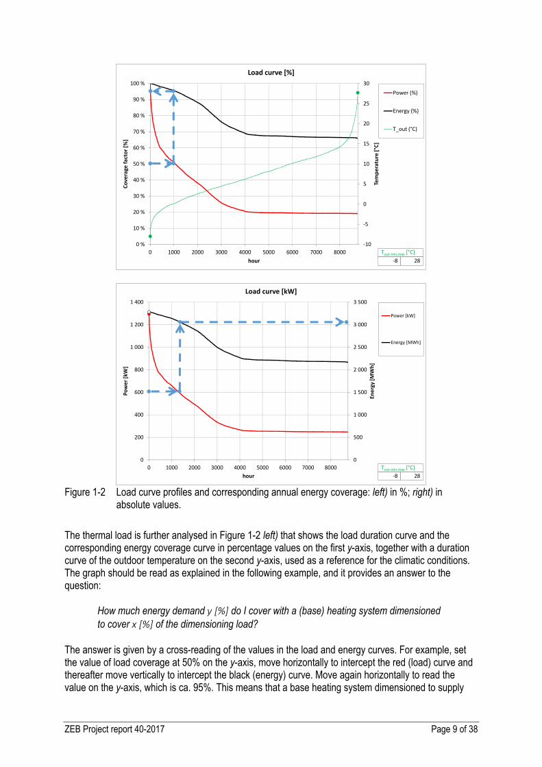
Figure 1-2 Load curve profiles and corresponding annual energy coverage: left) in %; right) in

absolute values.

The thermal load is further analysed in Figure 1-2 left) that shows the load duration curve and the corresponding energy coverage curve in percentage values on the first y-axis, together with a duration curve of the outdoor temperature on the second y-axis, used as a reference for the climatic conditions. The graph should be read as explained in the following example, and it provides an answer to the question:

How much energy demand y [%] do I cover with a (base) heating system dimensioned to cover x [%] of the dimensioning load?

The answer is given by a cross-reading of the values in the load and energy curves. For example, set the value of load coverage at 50% on the y-axis, move horizontally to intercept the red (load) curve and thereafter move vertically to intercept the black (energy) curve. Move again horizontally to read the value on the y-axis, which is ca. 95%. This means that a base heating system dimensioned to supply

-10

-5

0

5

10

15

20

25

30

0 %

10 %

20 %

30 %

40 %

50 %

60 %

70 %

80 %

90 %

100 %

0 1000 2000 3000 4000 5000 6000 7000 8000

Tem

pera

ture

[°C]

Cove

rage

fact

or [%

]

hour

Load curve [%]

Power (%)

Energy (%)

T_out (°C)

Tout-min,max [°C]-8 28

0

500

1 000

1 500

2 000

2 500

3 000

3 500

0

200

400

600

800

1 000

1 200

1 400

0 1000 2000 3000 4000 5000 6000 7000 8000

Ener

gy [M

Wh]

Pow

er [k

W]

hour

Load curve [kW]

Power [kW]

Energy [MWh]

Tout-min,max [°C]-8 28


50% of the dimensioning load would cover ca. 95% of the annual energy demand, leaving barely 5% to be covered by the top (back-up) heating system. Knowledge of such values is important when designing the heating system because it affects its cost and performance. The investment cost normally increases proportionally with the installed capacity (higher capacity = higher cost), while the part load efficiency normally decreases inversely proportional to the installed capacity, and with it the operational cost goes up (higher capacity = lower part-load efficiency = higher operational cost). It is therefore convenient to under-dimension the main heating generator (the base heater, e.g. the heat pump) in order to have it operating closer to its nominal capacity and thus reduce both investment and operational costs. On the other hand, the top heater (e.g. electric immersion resistance) is normally chosen to be significantly cheaper in installation cost, but the price to pay for it is that its operational performance is poorer. Therefore, a minimization of the global cost (investment and operation and maintenance) for the entire heating system (base and top heaters) should be sought as a balance between a low base-heating dimensioning and a low top-heating operation. As a rule of thumb – for example for heat pumps, though similar considerations are valid also for boilers and CHP units – it is often good practice to dimension the base heating system to cover about 40-60% of the maximum load. However, the shape of the load duration curve in highly energy efficient buildings is substantially different than in conventional buildings. Furthermore, the storage will also play an important role in hedging between nominal and part-load efficiencies, at the cost of some storage losses. The proper dimensioning of the heating system is a task for future work, for which the graphs shown here will be the main input. In this study it is assumed that the base heating system is dimensioned for a nominal capacity of 600 kW. Figure 1-2 right) shows that choosing a base heating system with a capacity of 600 kW (ca. 50% of the dimensioning load) would cover more than 3.0 GWh of yearly energy demand (i.e. more than 90% of the total). Based on discussions with the project partners, three possible solutions are investigated for the energy system of Zero Village Bergen:

1. District Heating (DH) 2. Biomass fired Combined Heat and Power (Bio CHP) 3. Ground Source Heat Pump (GSHP)

The details of each system are discussed in the following chapters. For all three solutions it is assumed that there is a local thermal network (nærvarme system) connecting the buildings with the energy central. In the case of DH (fjernvarme) it is assumed that the central is a substation of the city district heating system and that the entire Zero Village Bergen is consideredto be a single node.


2 Key Performance Indicators

The following Key Performance Indicators (KPI) are evaluated in order to compare the three systems: Technical system performance

o Thermal Power: Thermal capacity Energy: Thermal efficiency

o Electric Power: Generation Multiple (GM) Energy: Self-consumption

Systems comparison o ZEB target

Energy demand Carbon emissions

o System cost Investment cost Operational cost Global cost

When comparing the three systems against one another, in Chapter 4, only the last two sets of indicators will be considered: ZEB target and System cost. This is because the Technical system performance indicators either do not have an implicit good-or-bad value (e.g. thermal capacity) or such value is already embedded in the other indicators. For example, higher thermal capacity is associated with higher investment cost while higher thermal efficiency – as well as higher electric self-consumption, as discussed later – is associated with lower operational cost; therefore such effects are already embedded in the indicators of System cost. The first set of indicators (Technical system performance) is discussed in Chapter 3. These indicators address both thermal and electric properties of the system and provide useful information for the design of the system (power indicators) and for its operation (energy indicators). For the thermal properties, the power indicator is the thermal capacity. This is given for both the base- and the top-heating system, as well as their coincident peak. The energy indicator is the overall thermal efficiency of the system, including both base- and top-heating, considering their actual (simulated) pattern of operation. For the electric properties, the power indicator is the Generation Multiple (GM), which is the ratio between the peak export and the peak import of power to and from the grid. The GM expresses how much larger the connection capacity needs to be due to electricity export to the grid (from local generation), as compared to the maximum electricity import from the grid. In buildings without local generation the GM = 0 by definition. If GM < 1 it means that the dimensioning parameter for the grid connection is still the load. But with larger PV systems installed (and eventually with the contribution from CHP too) one may have GM > 1. This implies that the local electric grid dimensioning capacity might be determined by the PV peak generation rather than by the peak load. Additionally, the GM may have a meaning for the operational cost too in the future, when the grid tariff is expected to become considerably more dependent on the power demand (maximum capacity required, either in import or in export) than on energy demand (total amount of electricity flowing through the grid). The electric energy indicator is the self-consumption, which means the amount of locally generated electricity that is instantaneously consumed by the buildings. Note that storage is not considered here,


neither as direct electric storage (e.g. in a battery) nor as indirect thermal storage (e.g. preheating of a water tank to avoid future import of electricity). Why is self-consumption important? Due to asymmetric prices of purchased (imported) and feed-in (exported) electricity, there is an economic incentive for the user to improve self-consumption. Example:

• Electricity imported from the grid costs 90 øre/kWh (spot price + grid tariff + taxes) • Electricity exported to the grid receives 30 øre/kWh (spot price only) Result: There is an incentive to maximize self-consumption

Different heating system technologies tend to have different matches with the PV generation, therefore different levels of self-consumption. The last two sets of indicators (ZEB target and System cost) are techno-economic indicators assumed to be have a significant impact in the choice of the energy system for Zero Village Bergen, and are discussed in Chapter 4. The ZEB target indicators express the ability of a system to meet the target of either "zero energy" or "zero emission". Both options are considered, even though "zero emission" is given higher importance because Zero Village Bergen is also a pilot project of the Zero Emission Buildings (ZEB) research centre. It should be noted that only the operational phase is considered here (no embodied energy/emission). In the classification of the ZEB centre, the ambition level of Zero Village Bergen is therefore at ZEB-O, see ZEB (2016b) [2]. The system cost indicators express the ownership cost of the energy system in the different phases of its economic lifetime, assumed to be 30 years. It is assumed that the global cost has a higher importance because it summarizes both investment and operational costs over the economic lifetime, duly discounted and expressed in terms of Net Present Value (NPV). The Technical system performance indicators are analyzed first, and presented in Chapter 3. The ZEB target and System cost indicators are (partly) built upon the technical system performance results and are presented in Chapter 4.


3 Technical system performance

In this chapter only the residential buildings are considered. This is due to the fact that, as explained in ZEB (2016a) [1], only the thermal demand of the residential buildings is actually simulated; while the demand for the non-residential buildings (offices, shops and kindergarten) is taken from measurements. However, in Chapter 4 adjustments are made in order to evaluate the performance of the whole Zero Village Bergen. The calculations are performed using the building simulation software IDA ICE1 and post processing in Excel for generating relevant graphs and indicators; see ZEB (2017) [3] for more details.

3.1 District Heating (DH)

The cost of the actual distribution grid (piping etc.) is assumed equal for all cases. Here only the heating central cost is included, assuming this is a substation for connection to the city-wide district heating system of Bergen. The carbon emission factor assumed here for the DH system is discussed in Chapter 4.1.2. 3.1.1 Performance results

The nominal data used as input for the DH system are:

Thermal capacity: unlimited Thermal efficiencies: 90% No base-top heater system; only DH seen as base heater

Based on these input, the IDA ICE model described in ZEB (2016a) [1] is simulated with a DH system. The results are summarized below. Table 3-1 reports the results for the key performance indicators considered. Table 3-1 System performance results for the DH system.

Performance indicator System

Thermal system

Base Heating Top Heating Energy carrier District heat -

Power Thermal capacity 1 390 kW - Coincident peak 1 390 kW

Energy Thermal efficiency 90 %

Electric system

Import Export

Power Coincident peak 730 kW 2 550 kW Generation Multiple (GM) 3.5

Energy Self-consumption 37 %

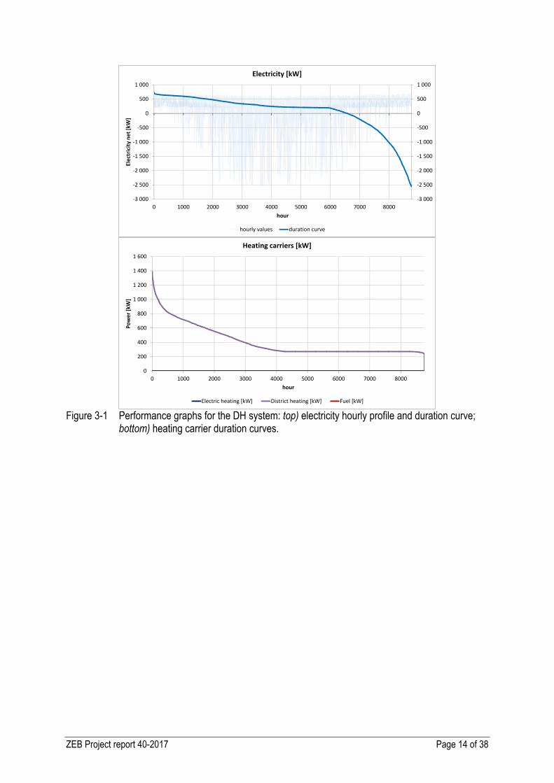
Figure 3-1 and Figure 3-2 show the annual profiles (hourly and monthly) and duration curves of both electricity and heating carriers use.

1 See http://www.equa.se/en/ida-ice.


Figure 3-1 Performance graphs for the DH system: top) electricity hourly profile and duration curve;

bottom) heating carrier duration curves.

-3 000

-2 500

-2 000

-1 500

-1 000

-500

0

500

1 000

-3 000

-2 500

-2 000

-1 500

-1 000

-500

0

500

1 000

0 1000 2000 3000 4000 5000 6000 7000 8000

Elec

tric

ity n

et [k

W]

hour

Electricity [kW]

hourly values duration curve

0

200

400

600

800

1 000

1 200

1 400

1 600

0 1000 2000 3000 4000 5000 6000 7000 8000

Pow

er [k

W]

hour

Heating carriers [kW]

Electric heating [kW] District heating [kW] Fuel [kW]


Figure 3-2 Performance graphs for the DH system: top) electricity monthly load and generation;

bottom) heating carriers monthly load.

3.2 Biomass Combined Heat and Power (CHP)

3.2.1 CHP technology

Combined Heat and Power (CHP) technologies suitable for direc usiof solid biomass as fuel (such as Organic Rankine Cycle, ORC, and Stirling engine) have rather low electric efficiencies in the order of 15-20%. The advantage in this case is that solid biomass also has a low CO2-factor. CHP technologies based on (bio)gas as fuel (such as gas turbines and gas internal combustion motors) have higher electric efficiencies, in the range 30-40%. The disadvantage in this case is that biogas also has a higher CO2-factor, thus counteracting the benefit of higher efficiency when looking at the ZEB balance. An alternative solution is to use a local gasifier in combination with a gas motor. In this case the fuel is again direct solid biomass, with a low CO2-factor, and the electric efficiency is at an intermediate level of ca. 20%. The disadvantage is that the thermal efficiency is reduced because of the gasification process. Another disadvantage is that the gasifier in itself is rather expensive, see Chapter 4.2.1. In this study it is assumed that the Bio CHP system is based on a local gasifier, as in the ZEB pilot Campus Evenstad. It is assumed that both performance and cost are similar to those in Campus Evenstad (2016) [4], even though this system is approximately 5-6 times as big and could therefore

0.0

1.0

2.0

3.0

4.0

5.0

6.0

7.0

Jan Feb Mar Apr May Jun Jul Aug Sep Oct Nov Dec

Elec

tric

ity [k

Wh/

m2]

Electricity monthly load and generationElectricity loadElectricity generation

mismatch factorsmonthly hourly

self-generation60 % 32 %

self-consumption70 % 37 %

GM (generation/load)4.0

GM (export/import)3.5

0.0

1.0

2.0

3.0

4.0

5.0

6.0

7.0


Elec

tric

ity [k

Wh/

m2]

Monthly heating loadElectric heatingDistrict heatingFuel heating

Electric heatingkWh/m2 a-

District heating41.8 kWh/m2 a

0.0 Fuel heating

kWh/m2 a


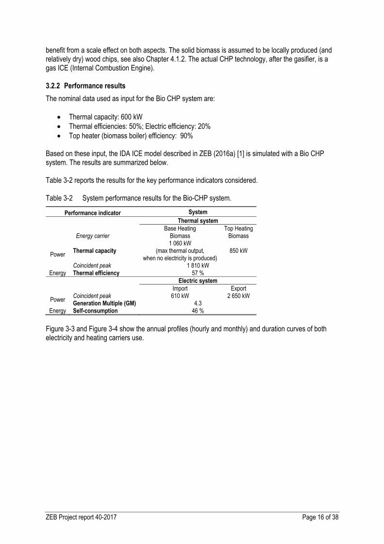
benefit from a scale effect on both aspects. The solid biomass is assumed to be locally produced (and relatively dry) wood chips, see also Chapter 4.1.2. The actual CHP technology, after the gasifier, is a gas ICE (Internal Combustion Engine). 3.2.2 Performance results

The nominal data used as input for the Bio CHP system are:

Thermal capacity: 600 kW Thermal efficiencies: 50%; Electric efficiency: 20% Top heater (biomass boiler) efficiency: 90%

Based on these input, the IDA ICE model described in ZEB (2016a) [1] is simulated with a Bio CHP system. The results are summarized below. Table 3-2 reports the results for the key performance indicators considered. Table 3-2 System performance results for the Bio-CHP system.


Thermal system

Base Heating Top Heating Energy carrier Biomass Biomass

Power Thermal capacity

1 060 kW (max thermal output,

when no electricity is produced) 850 kW

Coincident peak 1 810 kW Energy Thermal efficiency 57 %

Electric system

Import Export

Power Coincident peak 610 kW 2 650 kW Generation Multiple (GM) 4.3




Figure 3-3 Performance graphs for the Bio CHP system: top) electricity hourly profile and duration

curve; bottom) heating carrier duration curves.

-3 000

-2 500

-2 000

-1 500

-1 000

-500

0

500

1 000

-3 000

-2 500

-2 000

-1 500

-1 000

-500

0

500

1 000

0 1000 2000 3000 4000 5000 6000 7000 8000

Elec

tric

ity n

et [k

W]

hour

Electricity [kW]


0

200

400

600

800

1 000

1 200

1 400

1 600

1 800

2 000

0 1000 2000 3000 4000 5000 6000 7000 8000

Pow

er [k

W]

hour




Figure 3-4 Performance graphs for the Bio CHP system: top) electricity monthly load and generation; bottom) heating carriers monthly load.

3.3 Ground Source Heat Pump (GSHP)

In order to properly evaluate the technical performance of the GSHP system it was first necessary to properly simulate the borehole field. This is explained in the following section. 3.3.1 Borehole field simulation

As partner in this project, CMR2 has analyzed the geothermal properties of Ådland – the area around Bergen where Zero Village Bergen is planned to be built – and estimated the energy balance of several borehole field configurations, CMR (2016) [5]. For this analysis they used the software named "Earth Energy Designer (EED)" and used as input the data on thermal energy demand from ZEB (2016a) [1] – the same as used here. Such simulations consider both the thermal interaction between the boreholes in the field and the dynamic effects over several years. Figure 3-5 left) shows the resulting brine temperature in steady state conditions – after a simulation period of 25 years – for the particular configuration of a field made of 136 boreholes (in a 8 x 17 rectangle) each 250 meters deep.

2 Christian Michelsen Research institute.

0.0

1.0

2.0

3.0

4.0

5.0

6.0

7.0

8.0


Elec

tric

ity [k

Wh/

m2]







0.0

1.0

2.0

3.0

4.0

5.0

6.0

7.0

8.0

9.0


Elec

tric

ity [k

Wh/

m2]


Electric heatingkWh/m2 a-


66.4 Fuel heating

kWh/m2 a


Figure 3-5 Annual profiles of brine temperature in steady state conditions: left) results from EED, in

CMR (2016) [1]; right) results from the IDA ICE simulation.

The results from CMR (2016) [5] were used to calibrate the simulation in IDA ICE. In IDA ICE it is possible to simulate a borehole field with either a simplified or an advanced model. The latter is commercially available as an additional module. However, it was possible to simulate the borehole field with the simple model without a significant loss of confidence in the results thanks to the calibration performed, here briefly explained. First, the properties of a single borehole had to be specified. Figure 3-6 shows the IDA ICE user interface for the simple borehole model. The relevant parameters of such as borehole geometry and fluid (brine), piping and ground properties were set according to input from CMR (2016) [5]. The only exception was the borehole resistance; this was assumed to be 0.12 mK/W in CMR (2016) [4], while a previous field study had found typical values being in the range 0.06 – 0.08 mK/W, see Brekke (2003) [6]. The value used in the simulation was 0.07 mK/W.

Figure 3-6 IDA ICE interface for the simple borehole model.

In the IDA ICE simple version of the borehole model, there is no interaction between boreholes, so that the number of boreholes is not so relevant. Furthermore, the simple model only simulates one year and so does not reach steady state conditions. By means of trial-and error it was found that simulations assuming a certain number of such non-interacting boreholes3, each with properties as shown in Figure 3-6, gave a reasonable match of the yearly brine temperature compared to the results from EED.

3 In this case 100 boreholes.

Fluid temperaturePeak cool loadPeak heat load

Year 25JAN FEB MAR APR MAY JUN JUL AUG SEP OCT NOV DEC

Flu

id te

mpe

ratu

re [°

C]

5

4,5

4

3,5

3

2,5

2

1,5


This result is shown in Figure 3-5 right) for comparison. It should be noticed that while the result from IDA ICE is not perfectly at steady state (the value in December is not exactly the same as in January), the difference is deemed small enough to be acceptable. Furthermore, the result from IDA ICE is ca. 0.5 C lower than in EED throughout the year. This is a slight penalty for the heat pump system, which is thus simulated to operate with a source temperature of half a degree less than what it is actually expected to be. This means the heat pump performance is slightly underestimated. For differences between EDD and the IDA ICE advanced borehole module, reference is made to Kauppinen (2015) [7]. He concludes that the IDA ICE advanced model allows for a more detailed configuration than EED, with the option of exact borehole coordinates and tilt angles. 3.3.2 Performance results

The nominal data used as input for the GSHP system are:

Thermal capacity: 600 kW Thermal efficiency (COP): 3.8

(both at standard rating conditions: Tbrine_in 0° C, Twater_out 45° C) Top heater (electric) efficiency: 100%

Based on these inputs, the IDA ICE model described in ZEB (2016a) [1] is simulated with a GSHP system. The results are summarized below. Table 3-3 reports the results for the key performance indicators considered. Table 3-3 System performance results for the GSHP system.


Thermal system

Base Heating Top Heating Energy carrier Electricity Electricity

Power Thermal capacity 170 kW

(760 kW max thermal output) 490 kW

Coincident peak 620 kW Energy Thermal efficiency 4.18 (COP)

Electric system

Import Export

Power Coincident peak 1 110 kW 2 540 kW Generation Multiple (GM) 2.3




Figure 3-7 Performance graphs for the GSHP system: top) electricity hourly profile and duration curve;

bottom) heating carrier duration curves.

-3 000

-2 500

-2 000

-1 500

-1 000

-500

0

500

1 000

1 500

-3 000

-2 500

-2 000

-1 500

-1 000

-500

0

500

1 000

1 500

0 1000 2000 3000 4000 5000 6000 7000 8000

Elec

tric

ity n

et [k

W]

hour

Electricity [kW]


0

100

200

300

400

500

600

700

0 1000 2000 3000 4000 5000 6000 7000 8000

Pow

er [k

W]

hour




Figure 3-8 Performance graphs for the Bio CHP system: top) electricity monthly load and generation;

bottom) heating carriers monthly load.

0.0

1.0

2.0

3.0

4.0

5.0

6.0

7.0


Elec

tric

ity [k

Wh/

m2]







0.0

0.2

0.4

0.6

0.8

1.0

1.2

1.4

1.6

1.8


Elec

tric

ity [k

Wh/

m2]


Electric heatingkWh/m2 a10.1


0.0 Fuel heating

kWh/m2 a


4 Systems comparison

In this chapter, the three system are compared with respect to the key performance indicators on the ZEB target and System cost. The non-residential buildings of Zero Village Bergen are also included in this analysis. Since their energy needs were extrapolated from measurements and not simulated4, the corresponding delivered energy is calculated assuming the same overall thermal efficiency of each system, as shown in Table 3-1 to Table 3-3. Thus, the energy demand of non-residential buildings is added to that of the residential ones resulting from the simulations in IDA ICE, for both electricity and thermal carriers. Consequently, also carbon emissions and energy related costs are increased. However, no extra capital cost is considered because of the non-residential buildings. This is because the capital cost depends on the installed capacity, which in turn depends on the coincident peak power demand. As shown in ZEB (2016a) [1], the increase in coincident peaks –both thermal and electric – due to the non-residential load is small and in a first approximation this can be neglected without significant impact. It is assumed that the coincident peaks, and therefore the installed capacity and its investment cost, remain unchanged when adding the non-residential buildings to the analysis.

4.1 ZEB target

It should be noted that only the operational phase is considered here (no embodied energy/emission). In the classification of the ZEB centre the ambition level of Zero Village Bergen is therefore a ZEB-O, see ZEB (2016b) [2]. 4.1.1 Energy demand

Energy demand results for the three systems are presented and compared here. The values shown here refer to final energy use and are given per energy carrier. In order to make an overall energy assessment, the values should be converted into primary energy using specific conversion factors for each carrier. This is not done here, so that the energy demand does not represent a ZEB balance (in the sense of Zero Energy Balance). It is merely the starting point for calculating a ZEB balance in terms of carbon equivalent emissions, which is done in the next section. The results for energy demand are shown in Table 4-1 both as absolute values for the entire Zero Village Bergen (MWh/y) and as specific values for an average square meter of floor area (kWh/m2/y). The same results are also shown graphically in Figure 4-1. Table 4-1 Energy results for the three systems.

Energy table MWh/y kWh/m2/y

DH Bio CHP GSHP DH Bio

CHP GSHP

District Heat 3 778 41

Biomass 6 000 65

Electricity import 2 342 1 527 2 997 25 17 33

Electricity export 1 862 2 106 1 738 20 23 19

4 Sources of data are Lindberg and Doorman (2013) [8] and Lindberg et al. (2015) [9], and the aggregated data for the Zero Village Bergen are presented in ZEB (2016) [1].


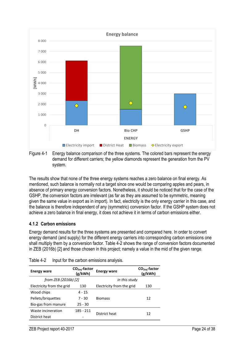
Figure 4-1 Energy balance comparison of the three systems. The colored bars represent the energy

demand for different carriers; the yellow diamonds represent the generation from the PV system.

The results show that none of the three energy systems reaches a zero balance on final energy. As mentioned, such balance is normally not a target since one would be comparing apples and pears, in absence of primary energy conversion factors. Nonetheless, it should be noticed that for the case of the GSHP, the conversion factors are irrelevant (as far as they are assumed to be symmetric, meaning given the same value in export as in import). In fact, electricity is the only energy carrier in this case, and the balance is therefore independent of any (symmetric) conversion factor. If the GSHP system does not achieve a zero balance in final energy, it does not achieve it in terms of carbon emissions either. 4.1.2 Carbon emissions

Energy demand results for the three systems are presented and compared here. In order to convert energy demand (and supply) for the different energy carriers into corresponding carbon emissions one shall multiply them by a conversion factor. Table 4-2 shows the range of conversion factors documented in ZEB (2016b) [2] and those chosen in this project; namely a value in the mid of the given range. Table 4-2 Input for the carbon emissions analysis.

Energy ware CO2eq-factor (g/kWh) Energy ware CO2eq-factor

(g/kWh) from ZEB (2016b) [2] in this study

Electricity from the grid 130 Electricity from the grid 130 Wood chips 4 - 15

Biomass 12 Pellets/briquettes 7 - 30 Bio-gas from manure 25 - 30 Waste incineration 185 - 211

District heat 12 District heat -

0

1 000

2 000

3 000

4 000

5 000

6 000

7 000

8 000

DH Bio CHP GSHP

ENERGY

[MW

h]Energy balance

Electricity import District Heat Biomass Electricity export


The conversion factor for electricity is 130 gCO2_eq/kWh given in ZEB (2016b) [2] and is used here; reference is made to the original source for details on how this factor has been calculated. It is here enough to mention that the value reflects an average for the lifetime of a building (set at 60 years), based on projections of the overall power system in Europe becoming nearly carbon free by 2050. The conversion factor for biomass is assumed to be 12 gCO2_eq/kWh, on the upper bound of the range for wood chips. Wood chips is the intended fuel as discussed in chapter 3.2.1; at the same time it is known from the experience in Campus Evenstad that the chips should be of rather good quality, meaning rather dry (< 30% relative humidity) for the gasifier to work properly. The conversion factor for district heating is also assumed to be 12 gCO2_eq/kWh. This may seem a rather generous assumption (in favor of district heating, making it look very "green"). In fact, there is an open discussion (in Norway) on which values to use. As discussed in ZEB (2016b) [2], the amount of emissions physically occurring when incinerating municipal waste are known with a certain confidence, at least as a national average, based on the average composition of the residual waste (the waste which is not going through differentiation). The unsettled argument is where such emissions should be allocated to: the waste management process itself or the district heat, which is a byproduct of the process, or both and then with which proportions? Here it is intentionally assumed the same conversion factor for district heating as for biomass (wood chips). The reason is pragmatic: on one side it neutralizes the difference between these two systems, so that any difference in the results will depend on other factors. On the other side it shows what happens, in terms of emissions, when assuming a nearly carbon free district heating system. This could be the case in Bergen when choosing to allocate zero emissions to the district heating. Indeed, ca. 95% of the energy sources in the district heating system is from waste incineration (although it might be more difficult to argue that the situation will remain such in future – for the next 60 years – if there is also going to be a significant expansion of the system). Alternatively, and most interestingly, it is same as assuming a local thermal network (nærvarmesystem) run by a biomass (wood chips) boiler. The results for carbon emissions are shown in Table 4-3 both as absolute values for the entire Zero Village Bergen (tonn CO2/y) and as specific values for an average square meter of floor area (kg_CO2/m2/y). The same results are also shown graphically in Figure 4-2. Table 4-3 Emission results for the three systems.

Emission table tonn_CO2/y kg_CO2/m2/y


CHP GSHP

District Heat 45 0.49

Biomass 72 0.78

Electricity import 304 199 390 3.31 2.16 4.24

Electricity export 242 274 226 2.63 2.98 2.46 Balance 108 -3 164 1.17 -0.04 1.78


Figure 4-2 Emission balance comparison of the three systems. The colored bars represent the energy

demand for different carriers; the yellow diamonds represent the generation from the PV system.

Figure 4-3 shows again the same information but this time in the form of a ZEB balance graph. In the x-axis are the equivalent imported emissions, due to the use of energy carriers; in the y-axis are the equivalent avoided emissions, due to export of electricity. The grey line represents a one-to-one balance, or a net zero balance between imported and exported (avoided) emissions. If the imported and exported values for a system meet above this line, the ZEB balance is satisfied; then Zero Village Bergen can be said to have zero emissions, or negative emissions. If the curves meet below the grey line, the ZEB balance is not satisfied; then Zero Village Bergen can be said to have nearly zero emissions. The solid lines represent the load-generation balance, i.e. the comparison of the total load and the total onsite generation, as if the two were related to completely separated and non-interacting systems. The dashed lines represent the import-export balance, i.e. considering the temporal interaction between load and onsite generation resulting from the hourly profiles.

0

50

100

150

200

250

300

350

400

450

DH Bio CHP GSHP

EMISSIONS

[ton

n CO

2]Emission balance

Electricity import District Heat Biomass Electricity export


Figure 4-3 ZEB balance graph for the three systems.

The results show that, with the given conversion factors, only the Bio CHP system meets the ZEB balance target, actually achieving a slightly negative balance.

4.2 System cost

The European cost optimal methodology specifies how to compare energy efficiency measures, measures incorporating renewable energy resources and packages of such measures in relation to their energy performance and the cost attributed to their implementation and how to apply these to selected energy reference buildings with the aim of identifying cost-optimal levels of minimum energy performance requirements. This is possible by converting all costs attributed to their implementation into global costs. Global cost calculation makes it possible to compare different energy supply solutions and other energy measures in an economic life cycle perspective. The global cost of an energy measure is the net present value of all costs associated with it during the defined calculation period, which may represent the economic or financial lifetime of the project. Long lasting equipment can be taken into account by subtracting its residual value at the end of the calculation period. The cost optimal methodology, as well as choice of values for the required parameters, is described in detail in Løtveit (2013) [10]. All costs shown in this section are excluded VAT (and other taxes on energy prices). 4.2.1 Investment cost

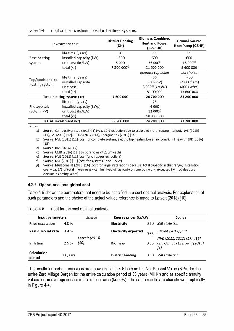
Table 4-4 shows the investment cost data used for the calculations, with notes on the data sources. It should be noticed that while the DH solution only consist of a base heating system, the Bio CHP solution incurs in significant additional costs for a biomass top heater (the cost would have been lower with an electric top heater, but then it would have no longer reached the ZEB balance). The GSHP solution, instead, incurs in significant additional costs for the borehole field.

0.0

1.0

2.0

3.0

4.0

5.0

6.0

0.0 1.0 2.0 3.0 4.0 5.0 6.0

expo

rted

[kg_

CO2/

m2]





Table 4-4 Input on the investment cost for the three systems.

Investment cost District Heating

(DH)

Biomass Combined Heat and Power

(Bio CHP)

Ground Source Heat Pump (GSHP)

Base heating system

life time (years) 30 15 15 installed capacity (kW) 1 500 600 600 unit cost (kr/kW) 5 000 36 000a) 16 000b) total (kr) 7 500 000c) 21 600 000 9 600 000

Top/Additional to heating system

biomass top boiler boreholes life time (years) 30 > 30 installed capacity 850 (kW) 34 000d) (m) unit cost 6 000e) (kr/kW) 400f) (kr/m) total (kr) 5 100 000 13 600 000

Total heating system (kr) 7 500 000 26 700 000 23 200 000

Photovoltaic system (PV)

life time (years) 25 installed capacity (kWp) 4 000 unit cost (kr/kW) 12 000g) total (kr) 48 000 000

TOTAL investment (kr) 55 500 000 74 700 000 71 200 000 Notes:

a) Source: Campus Evenstad (2016) [4] (+ca. 10% reduction due to scale and more mature market), NVE (2015) [11], IVL (2015) [12], IRENA (2012) [13], Energinet.dk (2012) [14]

b) Source: NVE (2015) [11] (cost for complete system, electric top heating boiler included). In line with BKK (2016) [15]

c) Source: BKK (2016) [15] d) Source: CMR (2016) [1] (136 boreholes @ 250m each) e) Source: NVE (2015) [11] (cost for chips/pellets boilers) f) Source: NVE (2015) [11] (cost for systems up to 1 MW) g) Source: Multiconsult (2013) [16] (cost for large installations because: total capacity in that range; installation

cost – ca. 1/3 of total investment – can be hived off as roof-construction work; expected PV modules cost decline in coming years)

4.2.2 Operational and global cost

Table 4-5 shows the parameters that need to be specified in a cost optimal analysis. For explanation of such parameters and the choice of the actual values reference is made to Løtveit (2013) [10]. Table 4-5 Input for the cost optimal analysis.

Input parameters Source Energy prices (kr/kWh) Source Price escalation 4.0 %

Løtveit (2013) [10]

Electricity 0.60 SSB statistics

Real discount rate 3.4 % Electricity exported - 0.35 Løtveit (2013) [10]

Inflation 2.5 %

Biomass 0.35 NVE (2011, 2012) [17], [18] and Campus Evenstad (2016) [4]

Calculation period 30 years District heating 0.60 SSB statistics

The results for carbon emissions are shown in Table 4-6 both as the Net Present Value (NPV) for the entire Zero Village Bergen for the entire calculation period of 30 years (Mill kr) and as specific annuity values for an average square meter of floor area (kr/m2/y). The same results are also shown graphically in Figure 4-4.


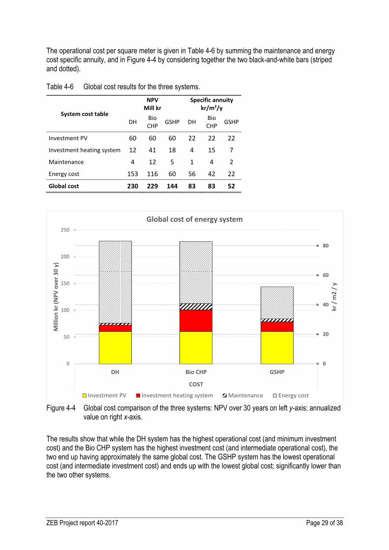
The operational cost per square meter is given in Table 4-6 by summing the maintenance and energy cost specific annuity, and in Figure 4-4 by considering together the two black-and-white bars (striped and dotted). Table 4-6 Global cost results for the three systems.

System cost table

NPV Mill kr

Specific annuity kr/m2/y


CHP GSHP

Investment PV 60 60 60 22 22 22

Investment heating system 12 41 18 4 15 7

Maintenance 4 12 5 1 4 2

Energy cost 153 116 60 56 42 22

Global cost 230 229 144 83 83 52

Figure 4-4 Global cost comparison of the three systems: NPV over 30 years on left y-axis; annualized

value on right x-axis.

The results show that while the DH system has the highest operational cost (and minimum investment cost) and the Bio CHP system has the highest investment cost (and intermediate operational cost), the two end up having approximately the same global cost. The GSHP system has the lowest operational cost (and intermediate investment cost) and ends up with the lowest global cost; significantly lower than the two other systems.

0

20

40

60

80

0

50

100

150

200

250

DH Bio CHP GSHP

COST

kr /

m2

/ y

Mill

ion

kr (N

PV o

ver 3

0 y)

Global cost of energy system

Investment PV Investment heating system Maintenance Energy cost


5 Sensitivity analysis

This chapter considers the effect on the ZEB balance of changing some parameters that are believed to have a significant effect on the results or that are known only with some uncertainty.

5.1 GSHP: DHW temperature

In the base case, the heat pump delivers hot water to the storage tank at 55 °C. This may vary upward, e.g. in case of improper commissioning, or downward, e.g. in case of adopting other solutions that guarantee legionella-free hot water at the tap. Table 5-1 and Figure 5-1 show the effect of the variants considered, with respect to the heat pump system performance and the ZEB balance, respectively. Table 5-1 Effect on the heat pump system performance of varying the hot water supply temperature.

Hot water temperature from heat pump

Heating system SPF (Seasonal Performance Factor)

Incl. the top heater

Seasonal COP (Coefficient Of Performance)

Heat pump only 55 °C (reference) 4.2 4.3

45 °C 4.6 4.7 65 °C 3.7 4.2

Figure 5-1 ZEB balance graph for the GSHP system with sensitivity analysis on DHW temperature.

This parameter does not have a significant influence on the ZEB balance, since all three variants remain largely in the 'nearly' ZEB area of the graph.

5.2 Bio CHP

This section analyses the effect of changing the CO2 factor for biomass and the electric efficiency of the CHP on the Bio CHP system; it also looks at the effect of a reduced investment cost by 50% and the adoption of a biogas based technology.

0.0

1.0

2.0

3.0

4.0

5.0

6.0

0.0 1.0 2.0 3.0 4.0 5.0 6.0

expo

rted

[kg_

CO2/

m2]



ZEB balance line GSHP - DHW 65C GSHP - DHW 45C GSHP - DHW 55C


5.2.1 CO2 factor

The CO2 factor for the biomass has been changed to represent different sources of biomass than the one assumed as reference: wood chips with a factor of 12 g_CO2/kWh. The low value for the CO2 factor corresponds to chips from local GROT5 = 4 g_CO2/kWh, while the high value corresponds to pellets of general EU origin = 30 g_CO2/kWh. For all values see Table 4-2. Figure 5-2 shows the effect of the variants considered.

Figure 5-2 ZEB balance graph for the Bio-CHP system with sensitivity analysis on the CO2 factor.

This parameter has some influence on the ZEB balance since it moves the balance point across the ZEB balance line by a significant amount. 5.2.2 Electrical efficiency

The electrical efficiency has been varied to test the effect of better or worse performance of the CHP unit. For any given technology (gas turbine, ORC, Stirling engine, or gas motor as in the case assumed here) the electric efficiency is highly dependent on how the unit is used, i.e. it depends on the thermal load it has to satisfy and the size of the thermal buffer (both affecting the hours of work at part load). The reference value is 20%, while the low and high value have been set at 15% and 25%, respectively. Figure 5-3 shows the effect of the variants considered.

5 Norwegian for GReiner Og Topper; in English: branches and tops, meaning from routine maintenance of woods

0.0

1.0

2.0

3.0

4.0

5.0

6.0

0.0 1.0 2.0 3.0 4.0 5.0 6.0

expo

rted

[kg_

CO2/

m2]



ZEB balance line Bio CHP @ 30 gCO2/kWhBio CHP @ 4 gCO2/kWh Bio CHP @ 12 gCO2/Kwh


Figure 5-3 ZEB balance graph for the Bio-CHP system with sensitivity analysis on the electrical

efficiency.

This parameter appears to have only a limited effect on the ZEB balance since it does move the balance point across the ZEB balance line but only of a moderate amount. The reason for it is that the thermal load for the Zero Village Bergen is rather small due to the energy efficient building envelopes, and it is the electric load that is dominant in determining the ZEB balance. 5.2.3 Halved investment cost

The investment cost for this technology is the highest and at the same time it is known with some uncertainty because the technology is rather new for the Norwegian market, at least for small scale applications such as the one assumed here. On the other hand, the unit required in this case is five to six times larger than the unit deployed at Campus Evenstad (2016) [4], which has been the source for the investment cost (of the gasifier, at least). The combined effect of a more mature market and a larger unit (than in Campus Evenstad) may result in a significant reduction of the investment cost. Assuming:

Halved investment cost (-50%) for the Bio CHP base heating system at 18 000 kr/kW (ref. 36 000 kr/kW)

The result is: Investment: 15.9 mill kr (ref. 26.7 mill kr) for the complete heating system; decreased investment

from more expensive to cheaper than the GSHP, see Table 4-4. Global cost: NPV over 30 years 202 mill kr (ref. 229 mill kr)

Unit cost: 73 kr/m2/y (ref 83 kr/m2/y); reduced global cost but still higher than the GSHP, see Table 4-6.

5.2.4 CHP unit with Biogas

If biogas is used as fuel there is no longer need for gasification on site. In this case both electrical and thermal efficiencies would be higher, because of not having the gasification process and related (thermal) losses on site. The investment cost would also be reduced significantly, while the fuel cost would increase significantly; also the CO2 factors increases.

0.0

1.0

2.0

3.0

4.0

5.0

6.0

0.0 1.0 2.0 3.0 4.0 5.0 6.0

expo

rted

[kg_

CO2/

m2]



ZEB balance line Bio CHP @ 15% el-effBio CHP @ 25% el-eff Bio CHP @ 20% el-eff


With the following assumptions:

CO2 factor: 25 gCO2/kWh (ref. 12 gCO2/kWh); lower limit, found up to 90 in literature, depending on source, ref. ZEB (2016b) [2]

CHP efficiencies: 33% electric and 55% thermal (ref. 20% - 50%); NVE (2015) [11]

The investment cost is significantly lower (the gasifier is expensive, not the gas-motor CHP as such): 11 000 kr/kW (ref. 36 000 kr/kW); NVE (2015) [11]

Fuel cost is significantly higher: 0.75 kr/kWh (ref. 0.35 kr/kWh); Vestfold kommune biogas report

These results are obtained: ZEB goal: almost achieve it with +20 gCO2/kWh (ref. -40 gCO2/kWh) Investment: 11.7 mill kr (ref. 26.7 mill kr) for the complete heating system; decreased investment

from more expensive to cheaper than the GSHP, see Table 4-4. Global cost: NPV over 30 years 284 mill kr (ref. 229 mill kr)

Unit cost: 105 kr/m2/y (ref 83 kr/m2/y); increased global cost when it was already the highest, see Table 4-6.

The ZEB balance remains approximately unvaried, while the economic results are contrasting. On one side the investment cost is reduced (eliminating the expensive local gasifier); on the other side the operating cost increases significantly due to the higher fuel price. The overall result is a worse global cost.

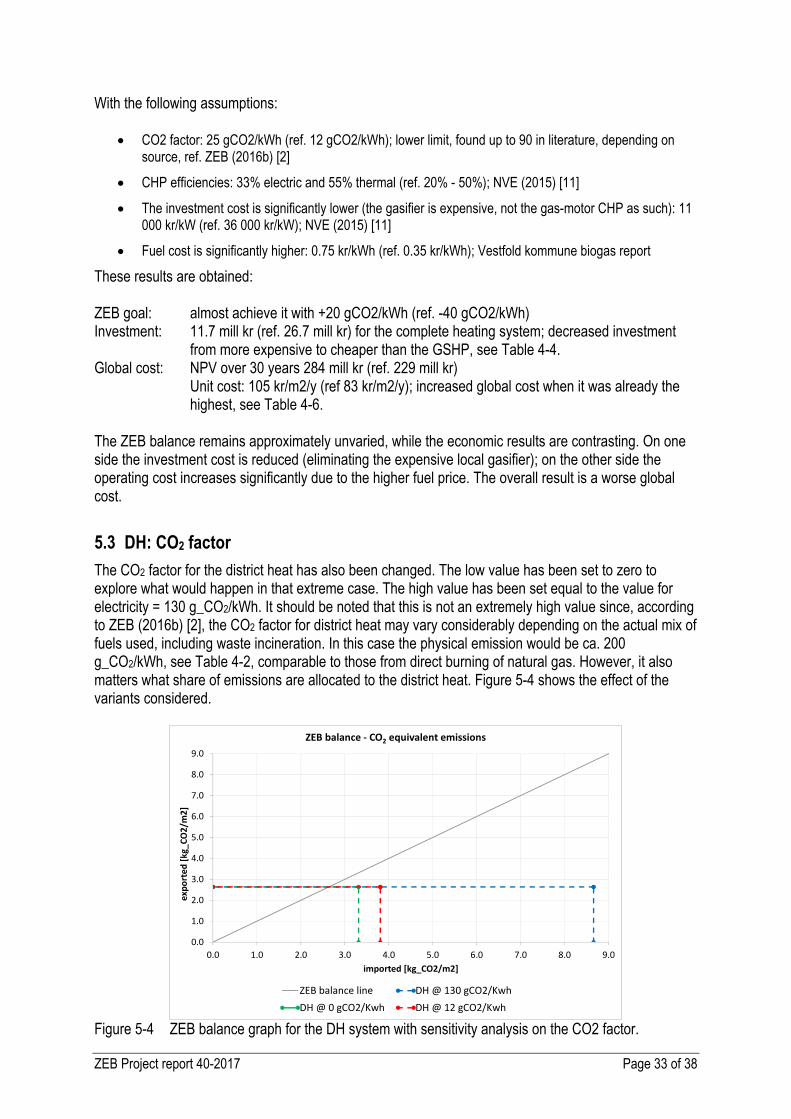
5.3 DH: CO2 factor

The CO2 factor for the district heat has also been changed. The low value has been set to zero to explore what would happen in that extreme case. The high value has been set equal to the value for electricity = 130 g_CO2/kWh. It should be noted that this is not an extremely high value since, according to ZEB (2016b) [2], the CO2 factor for district heat may vary considerably depending on the actual mix of fuels used, including waste incineration. In this case the physical emission would be ca. 200 g_CO2/kWh, see Table 4-2, comparable to those from direct burning of natural gas. However, it also matters what share of emissions are allocated to the district heat. Figure 5-4 shows the effect of the variants considered.

Figure 5-4 ZEB balance graph for the DH system with sensitivity analysis on the CO2 factor.

0.0

1.0

2.0

3.0

4.0

5.0

6.0

7.0

8.0

9.0

0.0 1.0 2.0 3.0 4.0 5.0 6.0 7.0 8.0 9.0

expo

rted

[kg_

CO2/

m2]



ZEB balance line DH @ 130 gCO2/KwhDH @ 0 gCO2/Kwh DH @ 12 gCO2/Kwh


This parameter has an asymmetric impact on the results. While the low value – which represents the lower bound, being zero – has a small effect on moving the balance point towards left, the high value – though not being the highest possible – has a large impact in pushing the balance point far to the right in the ZEB balance graph.

5.4 Relaxed ZEB definition

This section considers the effect of relaxing the ZEB definition to two levels: ZEB-O÷EQ and EPBD-ZEB. All figures in this section show both load-generation and import-export balances. It shall be noted that, according to the standardized wat of accounting for the energy performance of buildings (EPB) (ISO 52000-1 [19]) there is a difference between "physical boundary" and "assessment boundary", and only what goes into the "assessment boundary" goes into the ZEB balance. It follows that one could consider two types of import-export:

the "import/export" balance with respect to the "physical boundary", which is the real one, measurable in reality;

the "import/export" balance with respect to the "assessment boundary", which is what matters in the ZEB definition

All energy that is "exported" out of the "assessment boundary" goes to benefit some other use than those regarded as building-related in the EPB. It does not matter, for the ZEB definition, whether it "physically" leaves the building; it goes to serve other non-building-related purposes, regardless where they are: e.g. cooking in the house, PC in the office, freezers in the nearby supermarket, feed-in to the grid (evt. even beyond the local transformer). These differences are irrelevant as long as the ZEB definition encompasses all the energy used by the building, because in this case the assessment boundary corresponds to the physical boundary. However, the two differ from one another when a relaxed ZEB definition is adopted, and the effect of this is analyzed here. If the ZEB-O÷EQ6 definition applies, then the load due to electric equipment (plug loads) should not be considered in the balance. For the residential buildings this is easily applied, since such a load is known from ZEB (2016a) [1]. For the non-residential buildings, since only the total electric specific load is known from ZEB (2016a) [1] (equipment + lighting), it has been assumed that half of it should be considered. This is a conservative assumption because in reality the lighting load (the only one to be considered in a ZEB-O÷EQ definition) is less than 50%. The resulting ZEB balance is shown in Figure 5-5.

6 See [2] for further details.


Figure 5-5 ZEB balance graph for the three systems with relaxed ZEB definition: ZEB-O÷EQ.

If the EPBD-ZEB7 applies, then plug loads are not considered in the balance as with the ZEB-O÷EQ but additionally, also lighting is not considered for residential buildings. The resulting ZEB balance is shown in Figure 5-6.

Figure 5-6 ZEB balance graph for the three systems with relaxed ZEB definition: EPBD-ZEB.

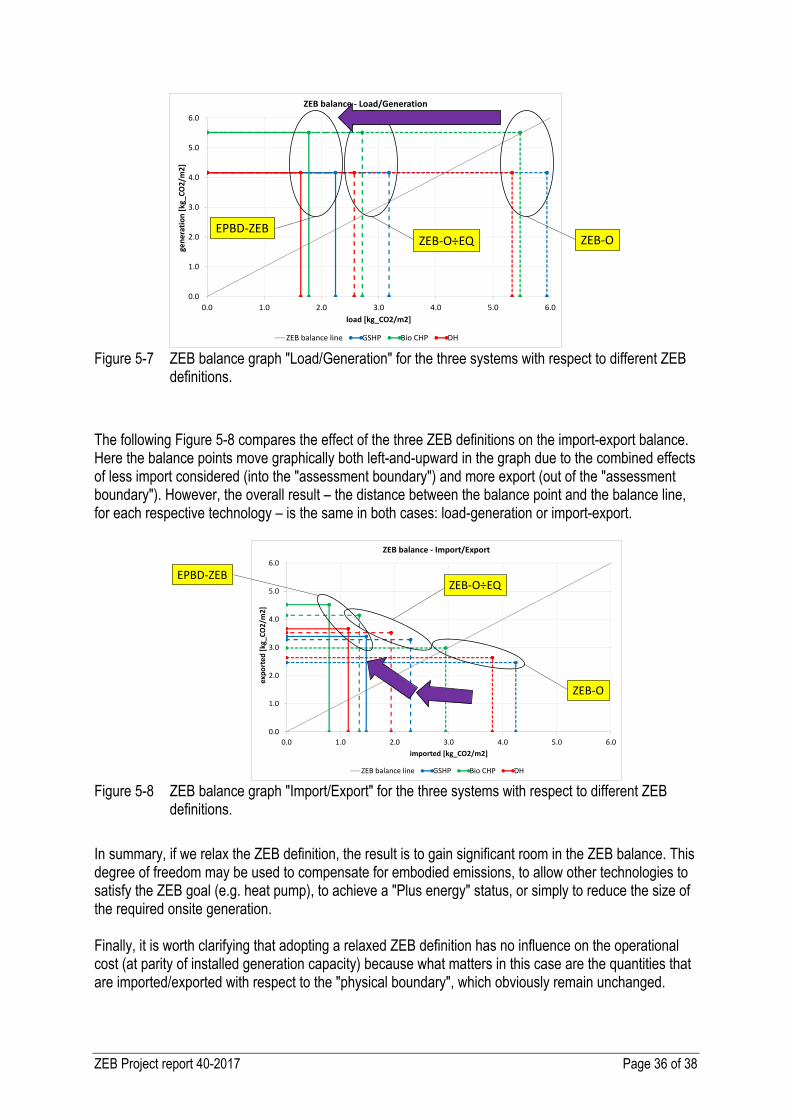
The following Figure 5-7 compares the effect of the three ZEB definitions on the load-generation balance. The overall effect is that the balance point – for each energy system – moves horizontally in the graph, towards left, as expected. Generation is always the same, it only varies what load is considered being inside the "assessment boundary".

7 EPBD = Energy Performance of Buildings Directive.

0.0

1.0

2.0

3.0

4.0

5.0

6.0

0.0 1.0 2.0 3.0 4.0 5.0 6.0

expo

rted

[kg_

CO2/

m2]




0.0

1.0

2.0

3.0

4.0

5.0

6.0

0.0 1.0 2.0 3.0 4.0 5.0 6.0

expo

rted

[kg_

CO2/

m2]





Figure 5-7 ZEB balance graph "Load/Generation" for the three systems with respect to different ZEB

definitions.

The following Figure 5-8 compares the effect of the three ZEB definitions on the import-export balance. Here the balance points move graphically both left-and-upward in the graph due to the combined effects of less import considered (into the "assessment boundary") and more export (out of the "assessment boundary"). However, the overall result – the distance between the balance point and the balance line, for each respective technology – is the same in both cases: load-generation or import-export.

Figure 5-8 ZEB balance graph "Import/Export" for the three systems with respect to different ZEB

definitions.

In summary, if we relax the ZEB definition, the result is to gain significant room in the ZEB balance. This degree of freedom may be used to compensate for embodied emissions, to allow other technologies to satisfy the ZEB goal (e.g. heat pump), to achieve a "Plus energy" status, or simply to reduce the size of the required onsite generation. Finally, it is worth clarifying that adopting a relaxed ZEB definition has no influence on the operational cost (at parity of installed generation capacity) because what matters in this case are the quantities that are imported/exported with respect to the "physical boundary", which obviously remain unchanged.

0.0

1.0

2.0

3.0

4.0

5.0

6.0

0.0 1.0 2.0 3.0 4.0 5.0 6.0

gene

ratio

n [k

g_CO

2/m

2]

load [kg_CO2/m2]

ZEB balance - Load/Generation

ZEB balance line GSHP Bio CHP DH

ZEB-OZEB-O÷EQEPBD-ZEB

0.0

1.0

2.0

3.0

4.0

5.0

6.0

0.0 1.0 2.0 3.0 4.0 5.0 6.0

expo

rted

[kg_

CO2/

m2]


ZEB balance - Import/Export

ZEB balance line GSHP Bio CHP DH

ZEB-O

ZEB-O÷EQEPBD-ZEB


6 Conclusions

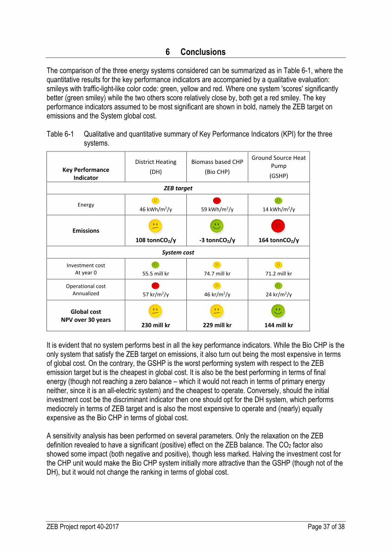
The comparison of the three energy systems considered can be summarized as in Table 6-1, where the quantitative results for the key performance indicators are accompanied by a qualitative evaluation: smileys with traffic-light-like color code: green, yellow and red. Where one system 'scores' significantly better (green smiley) while the two others score relatively close by, both get a red smiley. The key performance indicators assumed to be most significant are shown in bold, namely the ZEB target on emissions and the System global cost. Table 6-1 Qualitative and quantitative summary of Key Performance Indicators (KPI) for the three

systems.

Key Performance Indicator

District Heating (DH)

Biomass based CHP (Bio CHP)

Ground Source Heat Pump

(GSHP)

ZEB target

Energy 46 kWh/m2/y

59 kWh/m2/y

14 kWh/m2/y

Emissions 108 tonnCO2/y

-3 tonnCO2/y

164 tonnCO2/y

System cost

Investment cost At year 0

55.5 mill kr

74.7 mill kr

71.2 mill kr

Operational cost Annualized

57 kr/m2/y

46 kr/m2/y

24 kr/m2/y

Global cost NPV over 30 years

230 mill kr

229 mill kr

144 mill kr

It is evident that no system performs best in all the key performance indicators. While the Bio CHP is the only system that satisfy the ZEB target on emissions, it also turn out being the most expensive in terms of global cost. On the contrary, the GSHP is the worst performing system with respect to the ZEB emission target but is the cheapest in global cost. It is also be the best performing in terms of final energy (though not reaching a zero balance – which it would not reach in terms of primary energy neither, since it is an all-electric system) and the cheapest to operate. Conversely, should the initial investment cost be the discriminant indicator then one should opt for the DH system, which performs mediocrely in terms of ZEB target and is also the most expensive to operate and (nearly) equally expensive as the Bio CHP in terms of global cost. A sensitivity analysis has been performed on several parameters. Only the relaxation on the ZEB definition revealed to have a significant (positive) effect on the ZEB balance. The CO2 factor also showed some impact (both negative and positive), though less marked. Halving the investment cost for the CHP unit would make the Bio CHP system initially more attractive than the GSHP (though not of the DH), but it would not change the ranking in terms of global cost.


7 References

[1] ZEB (2016a) Zero Village Bergen – Aggregated loads and PV generation profiles, ZEB Project report 28. Authors: I. Sartori, S. Merlet, B. Thorud, T. Haug and I. Andresen.

[2] ZEB (2016b) A Norwegian ZEB Definition Guideline, ZEB Project report 29. Authors: S. M. Fufa, R. D. Schlanbusch, K. Sørnes, M. I. and I. Andresen.

[3] ZEB (2017) Guidelines on energy system analysis and cost optimality in early design of ZEB, ZEB project report. Authors: Igor Sartori, Sjur V. Løtveit, Kristian S. Skeie.

[4] Campus Evenstad (2016) Pilot project in the ZEB centre, data from personal communication with Statsbygg and Asplan Viak.

[5] CMR (2016) Termisk energilagring i berggrunnen med aktivt bidrag fra grunnvann – Zero Village Bergen, Christian Michelsen Research final report project nr. 311507. Authors: K. Midttømme, J. Kocbach, I. Henne, E. Bastesen.

[6] Brekke (2003) Energiuttak fra fjell - Et studium av data fra termisk responstesting, masteroppgave NTNU, Norway.

[7] Kauppinen, R. (2015) Analysis of building energy use and evaluation of long-term borehole storage temperature, Master thesis at KTH, Sweden.

[8] K.B. Lindberg and G. Doorman (2013) Hourly load modeling of non-residential building stock, IEEE PowerTech conference, 16-20 Jun., Grenoble, FR.

[9] K.B. Lindberg, J.E. Chacón, G. Doorman, D. Fischer (2015) Hourly Electricity Load Modelling of nonresidential Passive Buildings in a Nordic Climate, IEEE PowerTech conference, 29 Jun.-2 Jul., Eindhoven, NL.

[10] Løtveit, S.V. (2013) Cost Optimality of Energy Systems in Zero Emission Buildings in Early Design Phase, MSc thesis at NTNU, Trondheim.

[11] NVE (2015) Kostnader i energisektoren – Kraft, varme og effektivisering Norges vassdrags- og energidirektorat (NVE), Rapport nr. 2/2015 del 1.

[12] IVL (2015) Investment cost estimates for gasification-based biofuels production systems, IVL Swedish Environnmental Institute, Report nr. B2221.

[13] IRENA (2012) Biomass for Power Generation, The International Renewable Energy Agency (IRENA), Renewable Energy Technologies: Cost Analysis Series, Volume 1: Power Sector, Issue 1/5.

[14] Energinet.dk (2012) Technology Data for Energy Plants – Generation of Electricity and District Heating, Energy Storage and Energy Carrier Generation and Conversion, tRhe Danish electricity transmission and system operator (Energinet.dk), Report dated May 2012.

[15] BKK (2016) Estimates from BKK (local energy company), data from personal communication in this project.

[16] Multiconsult (2013) Kostnadsstudie, Solkraft i Norge 2013 – Priser, strømproduksjon og energikostnader, Multiconsult report for Enova (Norwegian Energy Agency), Dokumentkode 125340-RIEn-RAP-001

[17] NVE (2011) Kostnader ved produksjon av kraft og varme, Norges vassdrags- og energidirektorat (NVE), Håndbok nr. 1/2011.

[18] NVE (2012) Bioenergiressurser i skog – kartlegging av økonomisk potensial, Norges vassdrags- og energidirektorat (NVE), Rapport nr. 32/2012.

[19] ISO 52000-1 Energy performance of Buildings – Overarching EPB assessment. Part 1: General framework and procedures, ISO/TC 163, ISO/DIS 52000-1 dated 28/08/2015.

The Research Centre on Zero emission Buildings (ZEB)The main objective of ZEB is to develop competitive products and solu-tions for existing and new buildings that will lead to market penetration of buildings that have zero emissions of greenhouse gases related to their production, operation and demolition. The Centre will encompass both residential and commercial buildings, as well as public buildings.

Partners

NTNU www.ntnu.no

SINTEF www.sintef.no

Skanska www.skanska.no

Weber www.weber-norge.no

Isola www.isola.no

Glava www.glava.no

Protan www.protan.no

Caverion Norgewww.caverion.no

www.zeb.no

ByBo www.bybo.no

Multiconsult www.multiconsult.no

Brødrene Dahl www.dahl.no

Snøhetta www.snoarc.no

Forsvarsbygg www.forsvarsbygg.no

Statsbygg www.statsbygg.no

Husbanken www.husbanken.no

Byggenæringens Landsforening www.bnl.no

Direktoratet for byggkvalitetwww.dibk.no

DuPontwww.dupont.com

NorDan ASwww.nordan.no

Enovawww.enova.no

SAPA Building system www.sapagroup.com

Sør-Trøndelag fylkeskommunewww.stfk.no

Entra Eiendom ASwww.entra.no

Documents

Igor Sartori, Kristian S. Skeie, Kari Sørnes and Inger ... · Igor Sartori, Kristian S. Skeie, Kari Sørnesand Inger Andresen Zero Village Bergen Energy system analysis ZEB Project