Identifying Noise Shocks: a VAR with Data Revisions∗1

Riccardo M. Masolo† Alessia Paccagnini‡2

December 20, 20133

Abstract4

We propose a new VAR identification strategy to study the impact of noise shocks5

on aggregate activity. We do so exploiting the informational advantage the econo-6

metrician has, relative to the economic agent. The latter, who is uncertain about the7

underlying state of the economy, responds to the noisy early data releases. The former,8

with the benefit of hindsight, has access to data revisions as well, which can be used9

to identify noise shocks.10

By using a VAR we can avoid making very specific assumptions on the process driving11

data revisions. We rather remain agnostic about it but make our identification strategy12

robust to whether data revisions are driven by noise or news.13

Our analysis shows that a surprising report of output growth numbers delivers a persis-14

tent and hump-shaped response of real output and unemployment. The responses are15

qualitatively similar but an order of magnitude smaller than those to a demand shock.16

Finally, our counterfactual analysis supports the view that it would not be possible to17

identify noise shocks unless different vintages of data are used.18

JEL CODES: E3, C1, D819

KEYWORDS: Noise Shocks, Data Revisions, VAR, Impulse-Response Functions20

∗We are particularly grateful to Larry Christiano, Giorgio Primiceri, Roberto Motto and Efrem Castel-nuovo. We also thank Abi Haddow, Lena Koerber, Francesca Monti, Michele Piffer, Kate Reinold, KostasTheodoridis and Matt Waldron for their comments on early versions of the manuscript and Rhys Mendes forallowing us to cite his work. We would also like to thank participants at the XXI International Conferenceon Money, Banking and Finance, the 2013 SNDE Symposium, the 2013 Congress of the European EconomicAssociation, the 2013 Money Macro and Finance Conference, the 6th London Macroeconomic Workshopat LSE and seminar participants at Univesitat Pompeu Fabra. Part of this research was carried out whileRiccardo M. Masolo was a student at Northwestern University and a trainee at the European Central Bank,whose support is gratefully acknowledged. The views and opinions expressed in this work are solely thoseof the authors and so cannot be taken to represent those of the Bank of England or the European CentralBank.†Bank of England and Centre for Macroeconomics, Email: Riccardo.Masolo@bankofengland.co.uk‡University of Milano-Bicocca, Department of Economics, E-mail : alessia.paccagnini@unimib.it

1

1 Introduction21

Contrary to what is assumed in most macroeconomic models (e.g. Christiano, Eichenbaum,22

Evans 2005 and Smets and Wouters 2003) the state of the economy in not known for certain23

when economic decisions are made.24

The constant stream of revisions in many macroeconomic series confirms this view1 and a25

small but growing number of DSGE models try to account for the effects implied by imper-26

fect knowledge of the state of the economy, e.g. Lorenzoni (2009), Mendes (2007), Masolo27

(2011).28

These models are typically characterized by imperfect and heterogeneous information re-29

garding the state of the economy. As a result, agents attach weight even to noisy indicators30

of aggregate economic activity, which would be completely disregarded in a full-information31

environment.32

The precision of aggregate economic indicators plays a key role for at least two reasons.33

Firstly, it can reduce the overall uncertainty about the state of the economy. Secondly, it34

correlates the information available to different agents thus reducing the need for them to35

guess what the other agents’ assessment of the state of the economy might be.36

In such a setting, even noisy signals about the past are useful to economic agents, which37

makes the mapping to the data much more straightforward, because early data releases are38

the real-world counterpart of noise-ridden signals of past output growth in dispersed infor-39

mation models. As a result, a noise shock will have an impact on future decision-making,40

as is the case in Barsky and Sims (2012) and Blanchard, L’Huillier and Lorenzoni (2013)41

but not because it reveals something about the future but rather because it is genuinely42

informative about the current state of the economy.43

44

1Which has been explored in the context of policy analysis by Orphanides (2003) and Altavilla andCiccarelli (2011).

2

Dispersed-information models tend to be cumbersome to solve, hence Bayesian estimation is45

impractical. Melosi (2013) represents an attempt in this direction but restricts information46

dispersion to firms.47

The difficulty to bring dispersed information models to the data induced a dychotomy in the48

literature. On the one hand is a long series of works, dating back to Mankiw and Shapiro49

(1986) and including Arouba (2008)2, which try to analyze the statistical properties of data50

revisions, thus assessing the quality of early data vintages.51

On the other hand, modelers (e.g. Mendes (2007)) have produced impulse-responses of ag-52

gregate variables to noise shocks based on calibrated frameworks.53

In our opinion, the best attempt to quantify the impact of noise shocks in a VAR for the54

sake of comparison to a dispersed information model is in Lorenzoni (2009) who estimates55

a VAR in the tradition of Galı (1999) and Blanchard and Quah (1989). This class of VARs56

identifies a demand shock and a supply or productivity shock by assuming that only the57

latter has a permanent effect on the level of output. Lorenzoni (2009) attributes all the58

effects of the demand shocks he identifies in his VAR to noise. As he himself acknowledges,59

this is an extreme assumption because it attributes the effects of all shocks which do not60

have a permanent effect on the level of output, e.g. monetary and fiscal shocks, to noise.61

This strong assumption serves him well in his exercise because it works against his model62

but leaves open the possibility of finding a more accurate quantification of the effects of noise63

shocks on the macro aggregates, which is what we set out to do.64

Clearly related to our work is a recent paper by Blanchard, L’Huillier and Lorenzoni (2013)365

which estimates responses to noise shocks and shows that a VAR cannot separate out the66

impact of noise shocks in the context of a model in which information is imperfect. It is67

important to note that Blanchard, L’Huillier and Lorenzoni (2013) impossibility result4, i.e.68

2See Croushore and Stark (2001) for a summary.3Although their definition of noise is somewhat different, as described above.4Blanchard, L’Huillier and Lorenzoni (2013) section 2.2

3

their statement that a noise shock cannot be identified in the context of a VAR, crucially69

relies on the assumption that the econometrician has access to the same information as the70

agents or less. In our analysis, however, the econometrician has more information (at least71

in this dimension) than the agents because of the benefit of hindsight, i.e. the econometrician72

knows the state of the economy which was not known to the agent at the time the decision73

was made5. While one might argue that the true underlying state is never fully revealed, it74

seems reasonable to work under the assumption that successive revisions are more accurate75

than those available when decisions are made. As a consequence, the information set of76

the econometrician who carries out an ex-post analysis is richer6 than that of the economic77

agents.78

Note that information dispersion (not only information imperfection) is critical here. If all79

agents shared the same information, no matter how imprecise, then they would get to know80

aggregate endogenous variables (such as output) by a simple symmetry argument, which81

would negate the econometrician’s informational advantage or, at best, reduce it to one pe-82

riod7. When information is not the same across agents, though, agents will correctly not83

presume that other agents’ decisions will be the same as theirs, hence they will remain un-84

certain about the aggregate level of the endogenous variables. As a result, they will find a85

noisy signal, such as the early data release, useful.86

Related and complementary to the work by Blanchard, L’Huillier and Lorenzoni is a recent87

work by Forni, Gambetti, Lippi and Sala (2013). The latter proposes a way to identify the88

effect of noise shocks in the context of a model similar to that in Blanchard L’Huillier and89

5And this is not limited to having a longer sample as Blanchard, L’Hullier and Lorenzoni (2013) considerin Section 2.5. By observing the early and the latest vintages of data the econometrician observes whatin Blanchard, L’Hullier and Lorenzoni (2013) is the signal and what would correspond to true underlyingpermanent productivity in their setup.

6When we say richer we mean that the information set of the econometrician is not a subset of thatof the agent. We do not necessarily imply that the agent’s information set is contained in that of theeconometrician.

7Knowledge of exogenous process can be imperfect for a long time but when all agents are the same, theyget to know endogenous variables simply by setting them.

4

Lorenzoni but both papers assume the noise shock to affect a signal concerning some future90

exogenous process (i.e. technology) while we maintain the assumption that the noise shock91

”corrupts” early releases of past output growth, which is clearly endogenous. As a result we92

allow the noise shock to affect future (but not present) realizations of the variable it affects93

while this is not the case in Forni, Gambetti, Lippi and Sala (2013). In Forni, Gambetti,94

Lippi and Sala (2013) it is the agents’ learning that allows to uncover the impact of what95

they call ”noisy news”, while we take advantage of the econometrician’s richer information96

set (which we refer to as benefit of hindsight) to identify noise shocks to the early data re-97

leases. In a way, the two approaches are complementary in a way because the focus on two98

different but non-exclusive definitions of noise. Also note that our procedure does not run99

into the issue of non-fundamentalness because, from the econometrician’s perspective, the100

noise shock can be recovered by the difference between two observables8.101

102

So far we have described, why using data revisions might help overcome Blanchard, L’Huillier103

and Lorenzoni (2013) impossibility result. That comes at a cost, however. Data revisions104

are not nearly as well behaved as noise shocks are assumed to be in the context of theoretical105

models, as a vast literature shows (e.g. Arouba (2008)). To assume that the revision corre-106

sponds to the noise shock would not only imply that the model correctly captures the private107

sector agents’ behavior but also that the specific functional form of the noisy signal is an108

accurate representation of early data releases. In most theoretical models (e.g. Mendes 2007109

and Masolo 2011) the noise shock and the model-implied data revision correspond exactly.110

In reality we know things are more complicated, Clements and Galvao (2010) try to model111

the statistical properties of data revisions.112

Our VAR is much more flexible in this respect, in the original spirit of Sims (1980), in that113

8Section 3.2 discusses how our procedure is robust to the case in which the noise shock does not correspondexactly to the revision in the data.

5

it captures the essential transmission mechanism of a noise shock while not getting specific114

about the details of the data revision process. Indeed, we take advantage of the timing115

restriction arising from the noise shock impacting the early data release directly and true116

fundamentals only with a lag, through the decision-making process of the agents, while re-117

maining agnostic on the process for data revisions. We know from empirical studies, e.g.118

Arouba (2008), that characterizing the revision process as purely news-driven or noise-driven119

is problematic. The benefit of using a VAR is that we can try to make our identification120

robust to this.121

As the discussion in Section 3 clarifies, the use of a VAR is critical in this respect because122

it ensures the orthogonality of the noise shock to the final release of data even when the123

revision would not be (the news case).124

125

In sum, our analysis shows how a simple timing identification assumption can deliver sensi-126

ble results. For one thing, the qualitative responses of output and unemployment to a noise127

shock are in line with those of a demand shock, i.e. the responses of output and unemploy-128

ment are inversely related in response to a noise shock. In this sense, our analysis confirms129

the maintained assumption in Lorenzoni (2009). However, from a quantitative standpoint,130

the responses to noise shocks, while statistically significant, are much smaller than responses131

to demand shocks. This confirms the impression that considering the identified demand132

shocks as being exclusively driven by noise greatly over estimates their impact, which we133

quantify to be around 5-8 percent of the business cycle (as measured by the shares of the134

variances of output growth and unemployment explained by the noise shock).135

Following the suggestion in Rodriguez-Mora and Schulstadt (2007), we also introduce a mea-136

sure of investment in our VAR and find that the responses of output and unemplyment to137

noise shocks are still signficant and that, consistent with accepted business cycle evidence138

(e.g. see King and Rebelo (1999)) investment seems to be more volatile than output.139

6

We complete our analysis with a simple counterfactual exercise, aimed at illustrating how140

our identification crucially depends on what we deemed above the benefit of hindsight. If the141

econometrician did not have more information than the economic agent then our evidence142

confirms that the noise shock could not be recovered.143

In this sense we see our analysis as making better use of all the available information to144

assess the impact the uncertainty about the state of the economy might have on agents’145

decisions.146

147

The rest of paper comprises and overview of noise shocks in models with dispsersed in-148

formation in Section 2, followed by the description of our general setup in Section 3. A149

discussion of our estiamted VAR is in Section 4 while Section 5 illustrates our counterfactual150

experiment and Section 6 concludes the paper.151

2 Noise Shocks in Dispersed Information Models152

A recent series of dispersed information general equilibrium models, e.g. Lorenzoni (2009),153

Mendes (2007) and Masolo (2011), provide the ideal theoretical foundation to study noise154

shocks.155

In standard full information economic models (e.g. Christiano, Eichenbaum and Evans 2005156

or Smets and Wouters 2003), information about the past is irrelevant: the agents know the157

current state of the economy, hence they will not respond to any noisy information about158

the past.159

In reality, however, people are uncertain the state of the economy so they take advantage of160

published data about, say, GDP growth in recent quarters to increase the accuracy of their161

expectations of the current state of the economy. The very fact that such series get revised162

shows that those numbers are not fully accurate (especially for the most recent periods), yet163

7

they contain useful information for the economic agents.164

Dispersed information models capture exactly this. Because agents are uncertain about the165

state of the economy, they will respond to an informative, albeit noisy, signal about the state166

of the economy as it improves the accuracy of their predictions.167

Note that heterogeneous information is important in this process. If the state was imper-168

fectly known but information was the same across agents, once each of them made a decision,169

because of symmetry, he or she would know for certain that everyone else will have made the170

same decision, while when information differs across agents, the noisy early release increases171

the agents’ knowledge and also affects the correlation of the agents’ information set.172

Moreover, the precision of the signal will impact the quantitative response but will not pre-173

vent agents from responding to noise. The impact of the noise embedded in the signal will174

only die out as agents learn about the true fundamentals, i.e. they become able to separate175

the genuine movement in economic variables from the noise embedded in the preliminary176

release9.177

178

Models such as those mentioned above can typically be readily cast in a state-space10 form in179

which at least the observation equation is household specific (as denoted by the h subscript):180

Zt = Ψ1Zt−1 + Ψ0ut (1)

sht = Γ1Zt + Γ0ζht (2)

Equation (1) is the transition equation, which controls the evolution of the state of the econ-181

omy Zt while, sht characterizes the information set of the economic agents which comprises a182

sequence of signals defined as linear combinations of (aggregate) state variables plus idiosyn-183

9The speed of learning is obviously a matter of one’s preferred calibration in a model. One of the benefitsof our analysis is to cast light on the time span over which these effects are statistically significant.

10It is usually the case that more lags of the state variables are needed to solve a dispersed informationmodel. Typically they are stacked to form a first-order system.

8

cratic components (ζht). We allow for each agent to observe different bits of information but,184

in a linear setting, all the idiosyincratic components integrate out in the aggregate.185

On the contrary, the noise shock does not net out in the aggregate because it is observed by186

all agents, hence usually the noise shock will be a component of the vector ut11.187

188

Typically the noise shock corrupts information regarding output growth or productivity189

in a way that is meant to mimic early releases of output growth figures which are available190

to everyone and yet are never fully precise.191

Because all the agents have access to this type of signal, aggregate variables will respond192

to some degree to the unexpected inaccuracies in the reports of, say, output growth. As a193

result we can investigate the impact of noise shocks with no need for individual-level data194

or survey expectations.195

2.1 Timeline196

While forecasts of macroeconomic variables are certainly available, it is realistic to assume197

that agents will only receive signals about aggregate variables (which we can consider im-198

perfect measures rather than pure forecasts) not before the end of period of interest12, i.e.199

once the aggregate variable of interest has materialized.200

As a result the following timing pattern (depicted in Figure 1) arises naturally:201

1. The noise shock, which we will denote by vt, hits the economy.202

2. At the end of the period the economy-wide signal, denoted by (x0t , e.g. early release of203

output growth), which is affected by the noise shock, is released204

11In principle the noise component might be itself autocorrelated, in which case it will enter the state vectorZt, while ut will include the innovation to that same process. Moreover, because the variable impacted bythe noise shocks (e.g. an early release of output growht) is observed symmetrically by all agents in theeconomy the row of Γ0 corresponding to the noisy variable will comprise all zeros.

12Or equivalently at the beginning of the following period

9

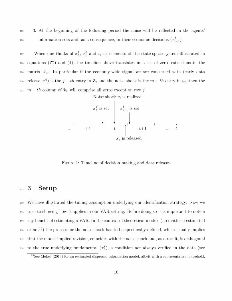
3. At the beginning of the following period the noise will be reflected in the agents’205

information sets and, as a consequence, in their economic decisions (xft+1).206

When one thinks of xft , x0t and vt as elements of the state-space system illustrated in207

equations (??) and (1), the timeline above translates in a set of zero-restrictions in the208

matrix Ψ0. In particular if the economy-wide signal we are concerned with (early data209

release, x0t ) is the j − th entry in Zt and the noise shock is the m− th entry in ut, then the210

m− th column of Ψ0 will comprise all zeros except on row j.211

-

t... t-1 t t+1 ...

?

xft is set

?

xft+1 is set

6

x0t is released

?

Noise shock vt is realized

Figure 1: Timeline of decision making and data releases

3 Setup212

We have illustrated the timing assumption underlying our identification strategy. Now we213

turn to showing how it applies in our VAR setting. Before doing so it is important to note a214

key benefit of estimating a VAR. In the context of theoretical models (no matter if estimated215

or not13) the process for the noise shock has to be specifically defined, which usually implies216

that the model-implied revision, coincides with the noise shock and, as a result, is orthogonal217

to the true underlying fundamental (xft ), a condition not always verified in the data (see218

13See Melosi (2013) for an estimated dispersed information model, albeit with a representative household.

10

Arouba 2008). On the other hand, the flexibility implicit in a VAR specification allows us219

to make our identification robust to situations in which revisions in the data turn out not to220

be orthogonal to the underlying fundamentals, as we will show below.221

3.1 Classical Noise222

We start by considering how our identification applies in the case in which the revision is

orthogonal to the fundamentals, a case we will refer to as classical noise.

Under this assumption, the early vintage of data (x0t ) equals the true or fundamental (xft )

plus the noise shock:

x0t = xft + vt vt ⊥ xft (3)

Appendix A shows that, given the state-space representation in equations (??) and (1), the

process governing xft can be expressed as:

xft = A(L)xft−1 +B(L)vt−1 + εt (4)

Where all the elements of equation (4) can be vectors, A(L) and B(L) are finite-order poly-

nomials in the lag operator and εt are the other shocks hitting the economy (e.g., in our

empirical exercise we will identify demand and supply shocks).

Equation (4) shows how past noise shocks affect the decision-making process of the agents in

the economy to the extent that they cannot separate them out from fundamentals. Agents in

the models will only observe a combination of noise and fundamentals, otherwise B(L) = 0,

i.e. they would not respond to noise.

Equations (3) and (4) define the evolution of the two set of variables we are interested

in, namely the early and the latest vintages of data.

11

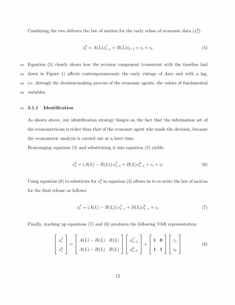
Combining the two delivers the law of motion for the early relase of economic data (x0t ):

x0t = A(L)xft−1 +B(L)vt−1 + εt + vt (5)

Equation (5) clearly shows how the revision component (consistent with the timeline laid223

down in Figure 1) affects contemporaneously the early vintage of data and with a lag,224

i.e. through the decision-making process of the economic agents, the values of fundamental225

variables.226

3.1.1 Identification227

As shown above, our identification strategy hinges on the fact that the information set of

the econometrician is richer than that of the economic agent who made the decision, because

the econometric analysis is carried out at a later time.

Rearranging equation (3) and substituting it into equation (5) yields:

x0t = (A(L)−B(L))xft−1 +B(L)x0t−1 + εt + vt (6)

Using equation (6) to substitute for x0t in equation (3) allows us to re-write the law of motion

for the final release as follows:

xft = (A(L)−B(L))xft−1 +B(L)x0t−1 + εt (7)

Finally, stacking up equations (7) and (6) produces the following VAR representation:

xft

x0t

=

A(L)−B(L) B(L)

A(L)−B(L) B(L)

xft−1

x0t−1

+

1 0

1 1

εt

vt

(8)

12

The matrix pre-multiplying [ εt vt ]′ simply highlights the timing pattern that emerges228

in our setup and which is true irrespective of the particular specification of the VAR. We229

postpone the complete identification of εt to our empirical exercise (see Section 4.2.2) because230

the identification of the other structural shocks inevitably depends on the variables included231

in the estimated VAR. In particular, we will explicitly identify demand and supply shocks232

using accepted identification restrictions (Blanchard and Quah, 1989).233

3.2 Prediction Error234

A vast empirical literature shows that revisions for some series are better characterized as

resulting from forecasting errors made by the agency which publishes early releases, e.g.

Mankiw and Shapiro (1986). We will sometimes refer to this situation as news .

The key difference with respect to the case illustrated above is that the revision is not or-

thogonal to fundamental xft , which makes it not a suitable candidate for a noise shock.

In this paragraph we illustrate how our VAR procedure actually mitigates this problem as

what we call noise shock is not (necessarily) the revision of data vintages, because it is or-

thogonal to the variables included in the VAR.

An exhaustive discussion of this issue would require the knowledge of the prediction models

used by the agencies which publish early vintages of data. Since that is not the case, we

will proceed with an example and discuss how our procedure is robust to a simple statistical

model.

Let us assume that a statistical agency receives a noisy signal on the true underlying eco-

nomic variable which takes on the following form:

x00t = xft + vt (9)

13

The key difference with respect to the case above is that now the agency correctly anticipates

that the data they collect are noise ridden (e.g. because they only collect a sample of the data

of interest) and so perform a filtering procedure before making them public. In particular, it

is reasonable to assume that they will consider the linear projection of the true underlying

variable onto the known signal so that the early release would take on the following form:

x0t = P[xft |x00t ] = φx00t = φxft + φvt (10)

Where the projection coefficient φ depends on the relative variance of noise in the signal x00t .

The key difference, relative to the case above is that now the data revision is not orthogonal

to the final release, in fact:

xft − x0t = (1− φ)xft + φvt (11)

As a consequence, it would be incorrect to take the revision as an indicator of the noise

shock. However, our VAR strategy provides a simple fix to this potential problem.

Under the maintained assumption that economic agents in the model know the data-generating

process (i.e. the state-space representation of the economy), the newly defined early release

would simply result in a different set of coefficients in the state-space representation in equa-

tions (1) and (2) but would otherwise not change the model which could be summed up

as:

xft = A(L)xft−1 + B(L)vt−1 + εt (12)

Where different filters A(L) and B(L) reflect the different coefficients in the state-space235

representation.236

Following the same steps as above, and using equation (10) as an alternative definition of the237

14

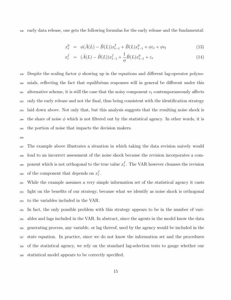
early data release, one gets the following formulas for the early release and the fundamental:238

x0t = φ(A(L)− B(L))xft−1 + B(L)x0t−1 + φεt + φvt (13)

xft = (A(L)− B(L))xft−1 +1

φB(L)x0t−1 + εt (14)

Despite the scaling factor φ showing up in the equations and different lag-operator polyno-239

mials, reflecting the fact that equilibrium responses will in general be different under this240

alternative scheme, it is still the case that the noisy component vt contemporaneously affects241

only the early release and not the final, thus being consistent with the identification strategy242

laid down above. Not only that, but this analysis suggests that the resulting noise shock is243

the share of noise φ which is not filtered out by the statistical agency. In other words, it is244

the portion of noise that impacts the decision makers.245

246

The example above illustrates a situation in which taking the data revision naively would247

lead to an incorrect assessment of the noise shock because the revision incorporates a com-248

ponent which is not orthogonal to the true value xft . The VAR however cleanses the revision249

of the component that depends on xft .250

While the example assumes a very simple information set of the statistical agency it casts251

light on the benefits of our strategy, because what we identify as noise shock is orthogonal252

to the variables included in the VAR.253

In fact, the only possible problem with this strategy appears to be in the number of vari-254

ables and lags included in the VAR. In abstract, since the agents in the model know the data255

generating process, any variable, or lag thereof, used by the agency would be included in the256

state equation. In practice, since we do not know the information set and the procedures257

of the statistical agency, we rely on the standard lag-selection tests to gauge whether our258

statistical model appears to be correctly specified.259

15

So, while the limited number of data points curtails the number of series and lags we can260

realistically include in our estimation, we find that using a VAR is more accurate than using261

data revisions directly (this is somewhat related to Rodriguez-Mora and Schulstad (2007)).262

4 VAR263

4.1 Baseline264

Our baseline VAR specification includes two vintages of quarterly (annualized) output growth265

and unemployment. Obviusly we need two vintages of output growth if we want to apply266

the identification scheme we laid down in the previous section, output being the key series267

subject to revisions. We only have one vintage of unemployment because the unemployment268

series is essentially never revised. Unemployment serves two key purposes in our context:269

I. Precisely because it is not revised it represents a good proxy for the data-publishing270

agency information set as it is readily available and clearly useful to assess economic271

conditions in real time. As such, we think it might help us making our identification272

robust to data revisions being driven by news, in the sense described in the previous273

section.274

II. Moreover, it allows us to identify demand and supply shocks with a long run restriction275

as in Blanchard and Quah (1989) as one of our goal is to show that using demand276

shocks as a proxy for noise shocks overestimates the impact of noise.277

We will later consider a larger set of variables (which includes a measure of investment),278

but we aim at keeping this exercise parsimonious for at least two reasons:279

1. We want to contribute to identification of noise shocks proposed by Lorenzoni (2009)280

who used a 2-variable VAR281

16

2. Including other variables subject to revisions would, potentially, increase the number282

of series (and of estimated parameters) much faster than in a traditional exercise using283

only the latest data release.284

We use de-meaned series so our estimation equation reads:

∆yft

uft

∆y0t

= β1

∆yft−1

uft−1

∆y0t−1

+ C

ν1t

ν2t

ν3t

(15)

Where C is the matrix identifying our structural shock which will be described below.285

4.1.1 Data Description286

For our empirical analysis, we consider the real GDP and the unemployment rate from the287

Historical Data Files for the Real-Time Data Set provided by the Federal Reserve Bank288

of Philadelphia (Croushore and Stark, 2001). The different vintages of data are available289

only from November 1965 to present. The quarterly vintages and quarterly observations290

of the Real GNP/GDP (ROUTPUT) is in Billions of real dollars, and seasonally adjusted.291

We take the first difference logarithmic transformation, so we consider it as a quarterly292

(annualized) growth rate14. Instead, the quarterly vintages and monthly observations of the293

Unemployment Rate (RUC) is in percentage points, seasonally adjusted. We transform our294

data from monthly to quarterly frequency considering the first observation of the quarter.295

We take levels of unemployment rate, without detrending15 it as discussed in Blanchard and296

Quah (1989). The investment, used in the robustness analysis, is given by the logarithmic297

14Using growth rates is motivated not simply by non-stationarity consideration but also by the fact that,as Rodriguez-Mora and Schulstad (2007) point out, it is easy to account for big long-term data revisions ingrowth rates (because typically affect one value which we substitute with the average of the previous andthe following quarter) than in level, because in this case the effect of the revision is essentially permanent.

15We do not detrend unemployment since our sample data does not show any deterministic or stochastictrends. Our longer sample from 1966 to 2006 considers different periods, from the Great Inflation to GreatModeration, with an evidence of no trend.

17

transformation of the ratio between the sum of Gross Private Domestic Investment (GPDI)298

and Personal Consumption Expenditures: Durable Goods (PCDG) and the Gross Domestic299

Product, 1 Decimal (GDP) as in Christiano et al. (2010). All these quarterly observations300

variables used to build the investment are provided by FRED Database of the Federal Reserve301

Bank of St. Louis.302

The VAR analysis, using one lag as suggested by the Schwartz Criterion, considers the303

quarterly sample from 1966:1 to 2006:4. We limit our sample until 2006, to leave a sufficiently304

long period after the end of the selected sample to be reasonably confident that the bulk of305

the revisions has ended by the time we carry out are analysis with a sufficiently long window306

for the end-of-sample observations. In fact, our final releases of output are those published307

in the third quarter of 201116 so we allow for about five years worth of revisions even for the308

data at the end of the sample. For the first release, on the other hand, we considered that309

derived from output level numbers published one quarter after the period of interest17, using310

a diagonal difference. That way it seems safe to consider that the agency had some time to311

collect data, reducing the forecasting component in the release and it also guarantees that312

such a number cannot affect the decisions of agents in the current period.313

4.2 Results314

4.2.1 Qualitative Similarities between Noise and Demand Shocks315

The discussion in Sections 2 and 3 delivers an identification assumption for the noise shock

which is the shock that contemporaneously affects the early relase of data only. This, in turn,

16Clements and Galvao (2010) entertain both the definition of final release as the latest available or thatoccurring a fixed number of quarters after the end of the period of interest (in their case 14 quarters, seemingto favor the latter because it is less affected by long-term revisions. On the other hand, Rodriguez-Moraand Schulstad (2007) seem to favor our approach. In any event, we find our approach a sensible benchmarkbecause the standard counterpart of our VAR would be one in which the latest releases available are used,not those published a certain fixed number of quarters after the end of the period of interest.

17The computer code we used to elaborate raw data can be requested to the authors.

18

pins down the third column of matrix C:

[C]3 =

0

0

c33

(16)

where [.]j refers to the j − th column of the matrix in brackets.316

The structure of the third column of matrix C implies that the our estimated noise shock ν3t317

will be orthogonal to all the variables included in the VAR except the current value of the318

first release (see the Appendix B for details).319

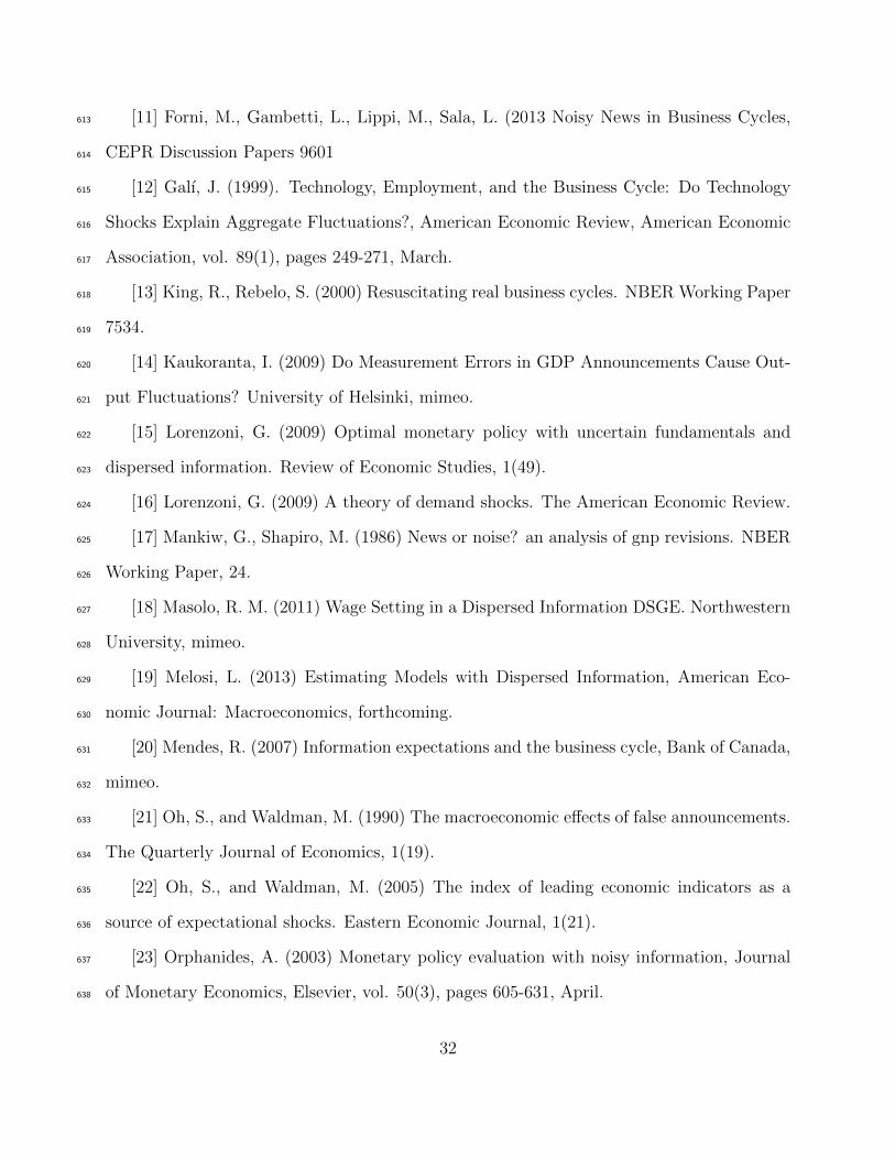
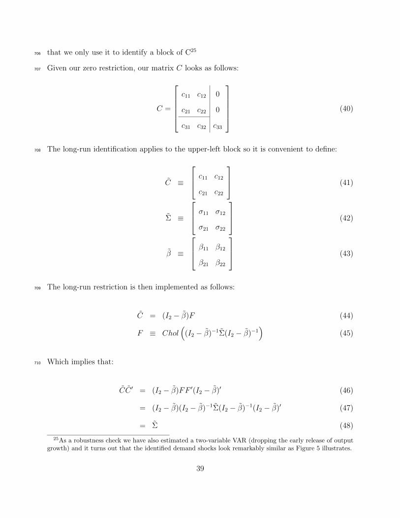
Figures 2 and 3 report the responses of final output (in log-levels) and unemployment to320

a positve noise shock, i.e. a situation in which the early data release is higher than the321

surprisingly higher than the fundamentals would imply.322

First, both of them are significant. Output appears to be statistically higher than it would323

otherwise be for about ten quarters, while unemployment is significantly below its long-run324

level for around three years.325

This means that an incorrect and unexpected early release of output figures tends to drive326

real underlying output in the same direction.327

However, it should be noticed that, not only the growth-rate of output converges back to328

zero but its log-level does as well, which is consistent with the idea that while noise shocks329

can be expected to produce variability at business cycle frequencies, no long-run effects330

on output seem likely, consistent with identification scheme in Lorenzoni (2009) who uses331

demand shocks as a proxy for noise shocks.332

Here we find, without imposing it, that, just like demand shocks in the Blanchard and Quah333

(1989) identification tradition, noise shocks do not affect the level of output in the long run.334

So, we find a qualitative similarity between noise shocks and demand shocks.335

Consistent with the idea of a demand shock is also the fact that the responses of output and336

19

unemployment have opposite signs, which one would expect when no productivity shocks337

are at play.338

Having listed the qualitative similarities of noise shocks with demand shocks we now turn339

to highlighting the important quantitative differences.340

4.2.2 Quantitative Differences between Noise and Demand Shocks341

To assess the quantitative differences between demand and noise shocks we need to identify342

both. Because of our variable selection, we can readily do so following Blanchard and Quah343

(1989). In particular, so far we have imposed two zero restrictions on the C matrix. A third344

restriction will identify all the shocks. While we leave a detailed derivation for appendix C,345

to build some intuition we report matric C here as well:346

C =

c11 c12 0

c21 c22 0

c31 c32 c33

(17)

The identification of the third column is discussed in the previous section (see equation 15).347

The third identifying restriction is imposed on the upper-left block of matrix C. Namely a348

long-run restriction is imposed, which restricts the demand shock not to have any long-run349

effect on the level of output (see Appndix C for details).350

The combination of the zero-restrictions to pin down the noise shock and the the long-run351

restriction to separate out demand and supply shocks also identifies the lower-left block of352

matrix C (the one that governs the response of the early data release to demand and supply353

shocks). In particular, given our restrictions, for C to satisfy CC ′ = Σ, i.e. for the covariance354

matrix of the structural shocks to equal the covariance of the estimation residuals, it has to355

20

be that:356

[c31 c32

]=

c11 c12

c21 c22

−1

Σ1:2,3

′

(18)

357

358

Having identified demand shocks we can now compare them with noise shocks. Figures359

4 and 5 report the same one-standard-deviation impulse responses to a noise shock, together360

with responses to a one-standard-deviation demand shock. In order to make the comparison361

more robust we report demand-shock responses identified as described in equation (16) and362

also demand shocks from a two-variable VAR (i.e. our baseline specification without the363

early output growth release, to be more consistent with Blanchard and Quah (1989) original364

setup). Interestingly, they deliver very similar results, suggesting that the inclusion of the365

early vintage of output growth does not materially affect the identification of demand shocks.366

On the one hand, these figures confirm the qualitative conclusions with drew above: demand367

and noise shocks both induce negatively correlated responses of output and unemployment368

(which suggests a sign restriction would not be enough to separately identify both).369

However, they also immediately reveal how the latter produce much larger effects on both370

output and unemployment, the demand shock being well outside the 95 percent confidence371

bands surrounding the responses to a noise shock. At their peak, responses to a demand372

shock are about three times as large as those to a noise shock, which gives us an indication373

of the magnitude of the overestimation of the effects of noise one would run into were they374

to apply a long-run identification scheme.375

This is what we were expecting as, by definition, long-run identification schemes are meant376

to capture any economic distrubances which do not have a long run effect on the level of377

output, e.g. most fiscal and monetary policy shocks.378

21

379

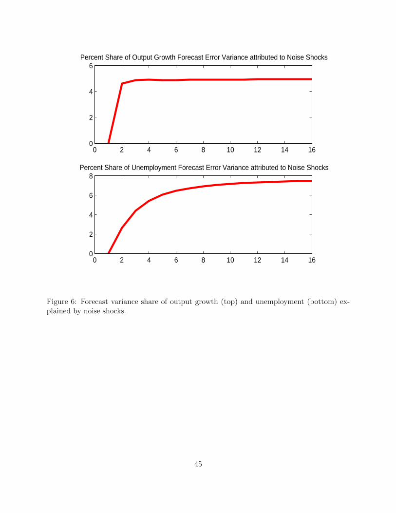
Looking at the variance decomposition for output growth and unemployment stenghtens380

our point further. Figure 6 illustrates how noise shocks can explain around 5 percent of the381

output growth dynamics and 7 to 8 percent of the movements in unemployment.382

Contrasting those numbers with the variance decompositions shown in Table 1 shows that383

the variance share of output growth and unemployment explained by the noise shock is about384

one order of magnitude smaller than that explained by demand shocks18. Which, once more,385

confirms the idea that using demand shocks as a proxy for the effects of noisy data releases,386

while qualitatively similar, greatly overestimates the impact of data revisions.387

This finding is consistent with Lorenzoni (2009) claim that his procedure overestimates the388

impact of noise shocks and provides a quantification of the overestimation, which appears to389

be large.390

4.2.3 Comparing the responses of different vintages391

So far, we have discussed, the differences and similarities in the responses of the final output392

growth release to demand and noise shocks.393

Now we turn to looking at the differences in the responses of the two vintages of output394

growth we consider in our analysis.395

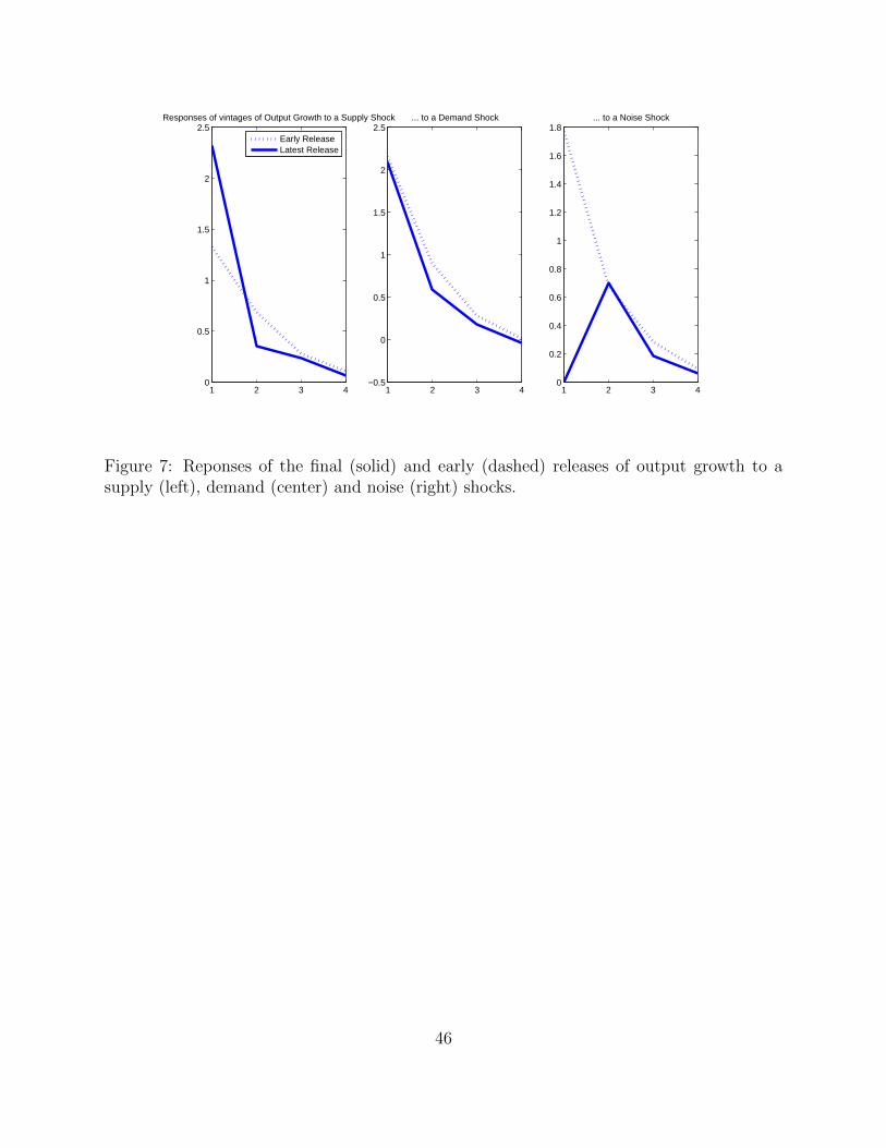
Figure 7 reports, side-by-side, the responses of the final (solid line) and early release (dashed396

line) of output growthto the Supply, Demand and Noise shocks respectively. Our identifica-397

tion restrictions explain why the final release of output growth does not respond contempo-398

raneously to a noise shock, but they do not directly restrict the response patterns to demand399

and supply shocks.400

Hence it is interesting to consider the striking difference in the two. When it comes to401

18This is in line with the finding that the impulse response is smaller by a factor of about three. If theMA representations of the responses to two different shocks (i.e. their impulse responses) are scaled by afactor of 3 the variance share of the shock with the bigger impluse response should be 9 times larger thanthan the other.

22

demand shocks the response of the early announcement and of the final release essentially402

overlap, while the early data release seems to underestimate the impact of a supply shock.403

While this is not conclusive evidence, it is consistent with the idea that because unemploy-404

ment is known in real time and is very closely linked to demand shocks, demand shocks are405

correctly reflected in the early data release already. The same is not true for supply shocks,406

which cannot be recovered by simply looking at unemployment (and even unemployment407

and the early data release) or, in other words, seem to take longer to be revealed.408

More generally, this pattern is consistent with the idea that demand shocks, such as some409

fiscal intervention, seem easier to spot right away than improvements in technology which410

are bound to take place at the individual firm level and require some time to become widely411

known.412

4.3 Alternative VAR Setup413

Rodriguez-Mora and Schulstad (2007) suggest that investment is a crucial variable when414

considering the impact of data revisions, which is reasonable given the forward-looking na-415

ture of investment decisions.416

Long-term projects, such as investment plans tend to be, are more susceptible to data im-417

perfections as they necessarily have to rely on forecasts of future conditions. On top of that,418

investment decisions are costly to reverse, once undertaken.419

Adding a measure of investment in our VAR we want to address two main points. First,420

we are interested in verifying if investment exhibits a significant response, somewhat along421

the lines of Rodriguez-Mora and Schulstad (2007). Secondly, introducing investment we can422

verify if the response of output to a noise shock is significant even when a measure of invest-423

ment is included in the VAR.424

Finally, adding an extra regressor further ”cleanses” our definition of noise shock for poten-425

tial correlations with variables which could enter the data-publishing agency’s information426

23

set. In particular, we make our noise shock orthogonal to our measure of lagged and current427

investment as well.428

429

Our definition of investment is similar to that in Altig, Christiano, Eichenbaum, Linde430

(2004), namely it is the log of the ratio of investment to GDP (in this case the final value of431

GDP). In other words, it is a measure of the investment-rate as a share of output.432

In particular, the investment is given by the logarithmic transformation of the ratio between433

the sum of Gross Private Domestic Investment (GPDI) and Personal Consumption Expen-434

ditures in Durable Goods (PCDG) and the Gross Domestic Product, 1 Decimal (GDP). All435

the quarterly-observation variables used to build the series for investment were taken from436

the FRED Database of the Federal Reserve Bank of St. Louis.437

4.3.1 Results438

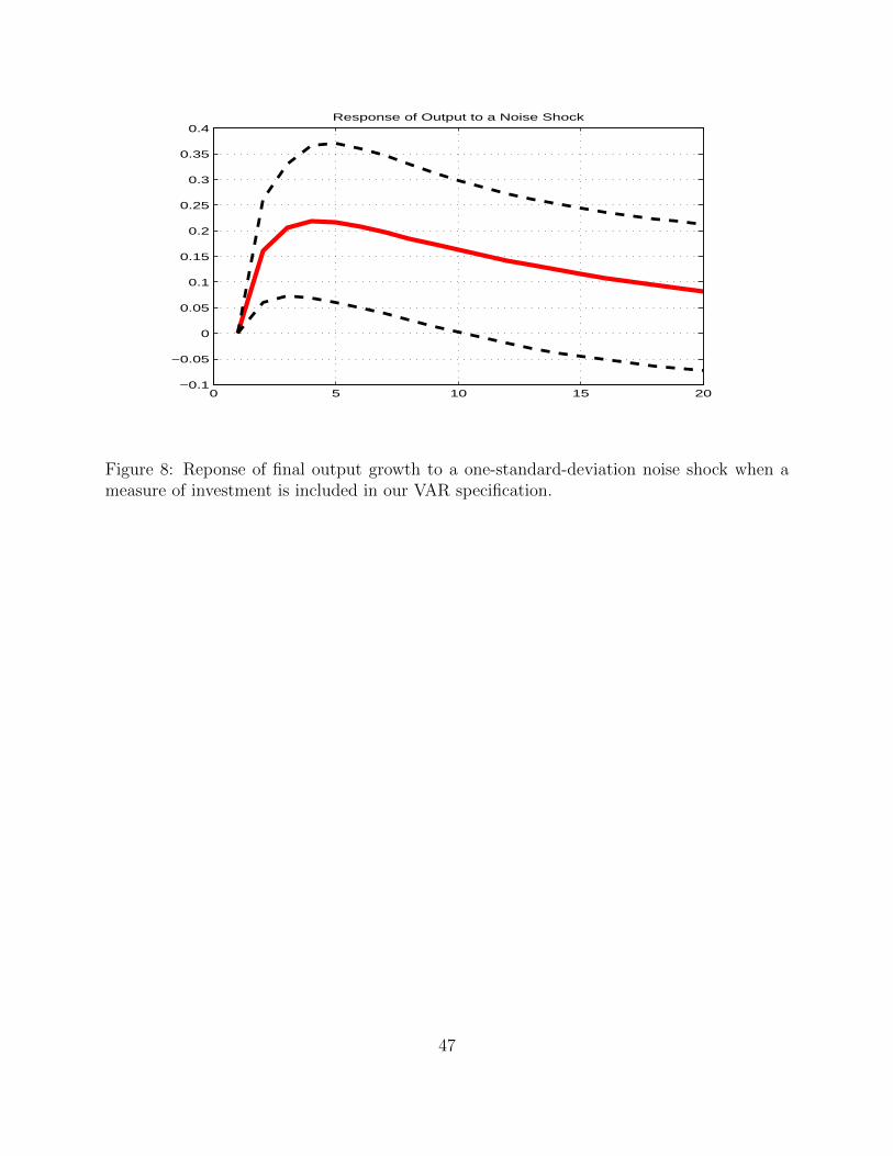
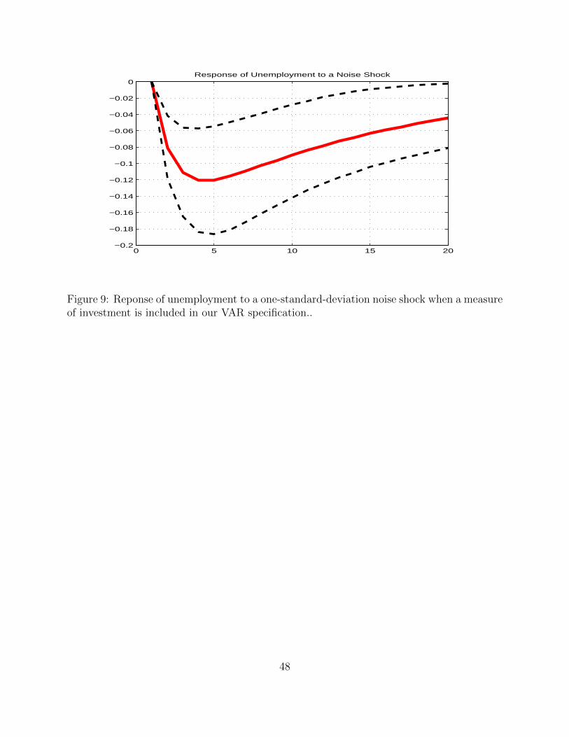
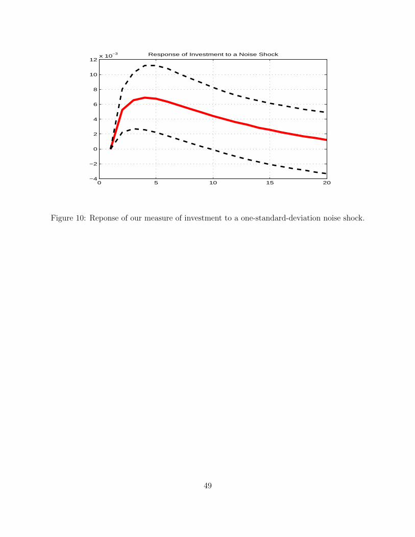
Results if Figure 8, 9 and 10 show that, once more, responses to revision shocks appear to439

be significant at business cycle frequencies.440

Interestingly, the size of the responses of output and unemployment is similar to that in441

the baseline setup we considered above, which appears to rule out the possibility that the442

response of output had to do with the omission of investment from the setup.443

At the same time, the investment rate is higher than average for about two years following444

an ”overly optimistic” early release of output growth numbers.445

In this respect, it should be noticed that it is not simply investment per se that increases,446

but investment as a share of output. Because output itself grows after a positive noise shock,447

this suggests that the level of investment increases in response to a noise shock more than448

output, consistent with basic business cycle facts that show how investment is positively449

correlated but more volatile than output (see King and Rebelo (2000)).450

Finally, the sheer size of the responses appears to support the idea that noise shocks produce451

24

real effects even when cleansed from any linear correlation of the revision with lagged and452

current investment rates. Turning to the analysis of the variance decomposition, Figure 10453

displays the variance-decomposition exercise for the specification which includes investment.454

As in the case above, the charts show the share of the forecast-error variance explained by455

revision shocks at different points into the future.456

Again the share of output growth variance explained levels off just below 5, the corresponding457

share being around 7 percent for unemployment and 6 percent for investment.458

In sum, adding investment does not change the big picture conclusions we drew for the case459

in which only output growth and unemployment enter the VAR specification. Moreover,460

broadly consistent with Rodriguez-Mora and Schulstadt (2007), we find that the response of461

investment is significant and, consistent with business cycle wisdom, we find it is actually462

larger than that of overall output.463

5 Counterfactual Analysis464

So far we have taken advantage of the fact that the information set of the econometrician is465

larger than that of economic agents who do not have the benefit of hindsight, i.e. they cannot466

observe the revision of the data series (at least by the time they make their decisions).467

Now we carry a different experiment which tries to highlight the benefits implicit in the468

extra information the econometrician has access to. Also, these experiments will allow us469

to discuss the key conclusion in Blanchard, L’Huillier and Lorenzoni (2013) because, given470

our estimated setup we can verify to which extent the noise shock can be recovered when471

revisions are not observed.472

473

Our counterfactual experiment relies on a state-space representation in which the state equa-474

tion is given by our estimated VAR, while, to keep things simple, the observation equation475

25

simply selects a subset of the variables. That means that we study a situation in which476

some, but potentially not all, of the state variables are observed. To keep things reasonably477

simple we assume that variables are either unobserved or fully known. The information478

imperfection aspect of the model comes in play only insofar as it is reflected by the early479

release being a noisy signal for true output growth.480

481

We will focus on our baseline specification so our state equation reads:482

∆yft

uft

∆y0t

= β1

∆yft−1

uft−1

∆y0t−1

+

c11 c12 0

c21 c22 0

c31 c32 c33

ν1t

ν2t

ν3t

(19)

Whereas the observation equation will change across the different scenarios but can be rep-483

resented as:484

ωt = Λ

∆yft

uft

∆y0t

(20)

Where the hypothetical agent/econometrician information set will consist of the timeless485

history of ωt observables and Λ is a q × 3 matrix of zeros and ones which selects 1 ≤ q ≤ 3486

of the 3 state variables. We refer to the different scenarios we define this way as observable487

combinations and, as already mentioned, for the sake of simplicity, we do not consider any488

additional type of shock/measurement error for this exercise.489

490

Given this setup, the remainder of this paragraph will try to assess whether it is possible to491

identify noise shocks with data available in real time.492

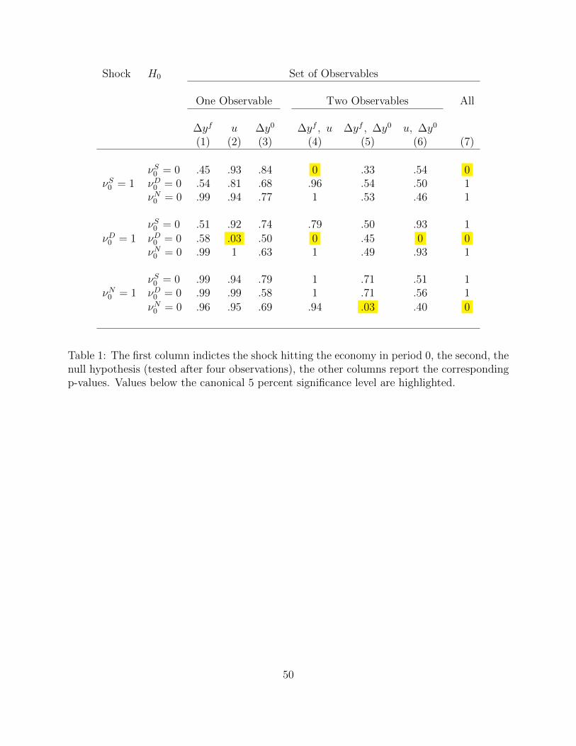
Table 1 reports the output of a simple set of hypothesis tests that try to assess how easy493

26

it is to correctly identify each of the three shocks given different sets of observables.494

The experiment works as follows:495

• We consider a one-standard-deviation shock for each type which produces three dif-496

ferent scenarios (hence three blocks in the table), while all the other shocks are zet to497

zero.498

• For each of the scenarios we test the null hypothesis that each of the shocks is zero,499

in turn, from the perspective of someone who has received signals ωt about that shock500

for four quarters19.501

• We repeat the tests for all the 7 possible combinations of observables.502

• We report p-values for all the possible combinations.503

To help the intution it is useful to start by considering column (7), i.e. the full infor-504

mation case20. Looking at the top section (νS0 = 1), the p-values take on value 0 when505

H0 : νS0 = 0, which is clearly not to be accepted, and one when the other two shocks are506

tested as being equal to zero. This is just a sanity check that compares our testing strategy507

against our identification strategy, in the sense that it shows that given the three series we508

observe the three shocks can be perfectly recovered.509

The p-value for the other six observable-combinations, on the other hand, can be taken as510

indications of how easy it is to recover a shock given incomplete information. Obviously511

some combinations (e.g. (1) and (4)) are less sensible than others (e.g. (3) and (6)) because512

they imply the final release of output is known while the first is not, but we report them all513

19The p-values are not independent of the number of observations agents receive prior to the test beingcarried out. We decide to consider the test being carried out 4 quarters after the shock but results seemrobust to increasing this number (because after a while there is quite little left to learn). Also, the p-valuesare not independed of the scale of the shock: we think of one-standard-deviation as a reasonable benchmarkto illustrate our point.

20In terms of the state space representation in equations (18) and (19), this corresponds to Λ = I3×3

27

for completeness.514

515

Highlighted in yellow are the cells in which the p-value comes out below the customary516

5 percent mark. Leaving aside the full information case which, as we said above, represents517

just a check of our procedure, a few interesting facts can be learnt.518

Unemployment reveals demand shocks. Indeed, all the observable-cobinations including un-519

employment allow to correctly reject the null that there was no demand shock when in fact520

there was one. Because demand shocks explain a massive share of the variance of unemploy-521

ment, observing it, even in isolation (observable-combination (3)), reveals what happened522

to demand. At a more general level, this reinforces our case to introduce unemployment523

because it shows how it can help identify at least one of the shocks, even when agents do524

not get to observe all the variables included in the VAR.525

Combination (4) is particularly relevant - we could call it the Blanchard-Quah observable526

combination - because it includes the two variables used in Blanchard and Quah (1989) and527

is indeed very similar to the pair used in Lorenzoni (2009) which features hours instead of528

unemployment. On the one hand it shows that the long-run identification scheme they first529

proposed is robust to a situation in which their VAR specification does not correctly capture530

the state of the economy, which, in our definition, includes the first release of output growth531

as well21.532

On the other hand, the bottom entry in the observable-combination (4) column reveals that533

this pair of observables does not help ”recovering” the noise shock. Hence, it reveals the534

shortcomings of identification strategies based on one vintage of data.535

In particular, the fact that the demand shock can be recovered while the noise shock (which536

in our controlled experiment is, by definition, contributing to the data-generation process)537

21This is also consistent with the fact that the demand shock identified in our baseline VAR and in thetwo-variable Blanchard and Quah specification are very close to each other (see Figure 5).

28

cannot highlights the dangers of considering demand shocks as a proxy for noise shocks.538

539

If combination (4) is the prototypical econometrician’s ex-post observable pair, combina-540

tion (6) can be thought to best represent real-time information. It turns out that knowing541

the early release and the unemployment figures allows to recover the demand shock only542

(because, as mentioned just above, unemployment ”reveals” the demand shock) but is no543

help in recovering a noise shock.544

In other words, the noise shock cannot be recovered by observing either real-time or ex-post545

data but requires both.546

Indeed, short of observing the entire three-variable state, the noise shock can only be re-547

covered observing two different vintages of output growth (combination (5)). Once more,548

this supports the general finding of Blanchard, L’Huillier and Lorenzoni (2013) that it is not549

possible to identify noise shocks observing just one vintage of data but also shows how the550

econometrician can take full advantage of a richer information set to uncover the effects of551

imprecise early data releases.552

6 Conclusion553

In a world in which there is uncertainty about the underlying state of the economy, early554

indicators of economic conditions can affect the decision-making process of the economic555

agents even if they are noise-ridden.556

We set out to try and quantify the impact of noise shocks, i.e. the component of early557

data releases that is unrelated to the contemporaneous true fundamental value. We did so558

exploiting the econometrician’s benefit of hindsight, i.e. the fact that she can observe both559

what in model would be considered the signal and the underlying fundamental on which560

the noise shock applies. This way we can overcome the impossibility result presented in561

29

Blanchard, L’Huillier and Lorenzoni (2013).562

Our identification strategy uses a timing assumption which restricts true economic funda-563

mentals to respond to noise shocks only with a lag, while the early data release is affected564

contemporaneously. This restriction arises naturally if one considers that early data releases565

(unless they are forecasts) can only be produced when the period at hand is over or, for our566

purposes, when the economic decisions have been made already.567

By carrying out our analysis in a VAR, we can afford to remain agnostic about the underly-568

ing drivers of data revisions, restricting only the timing of the responses as described above.569

Indeed, we show how our identification strategy can, under certain conditions, uncover the570

noise shock even when data revisions are driven by news, i.e. the revision is not orthogonal571

to the fundamentals.572

Our empirical exercise shows qualitative similarities between the responses to a noise shock573

and a demand shock, primarily the negative correlation of output and unemployment re-574

ponses, which was the proxy to a noise shock used in Lorenzoni (2009). However, the575

responses to noise shocks are much smaller (about a third in size at the peak) than those576

to demand shock, showing that using demand shocks as a proxy for identified noise shocks577

would over estimate the impact of imprecise data releaes on the business cycle. Our analysis578

quantifies the contribution of noise shocks to around 4-8 percent of the variance of output579

growth and unemployment.580

Following the analysis of Rodriguez-Mora and Schulstadt (2007), we also study the impact581

of the noise shock on investment and find that when we introduce a measure of investment582

in our VAR specification the responses of output and unemployment are roughly unaffected583

and investment as a positive and significant response.584

Finally, we consider a counterfactual experiment based on our estimated VAR, which sup-585

ports the view that noise shocks cannot be recovered unless different vintages of data are586

used.587

30

References588

[1] Altavilla, C., Ciccarelli, M. (2011) Monetary Policy Analysis in Real-Time. Vintage589

Combination from a Real-Time Dataset, CESifo Working Paper Series 3372, CESifo Group590

Munich.591

[2] Altig, D., Christiano, L., Eichenbaum, M., Linde J. (2011) Firm-specific capital,592

nominal rigidities and the business cycle. Review of Economic Dynamics, Elsevier for the593

Society for Economic Dynamics, vol. 14(2), pages 225-247, April.594

[3] Arouba, S. B. (2008) Data revisions are not well behaved. Journal of Money, Credit595

and Banking, 22.596

[4] Barsky, R. B., Sims, E. R. (2012) Information, animal spirits, and the meaning of597

innovations in consumer confidence. American Economic Review 102, 4,1343(1377).598

[5] Blanchard, O., Quah, D. (1989) The Dynamic Effects of Aggregate Demand and599

Supply Disturbances, American Economic Review, American Economic Association, vol.600

79(4), pages 655-73, September.601

[6] Blanchard, O., L’Hullier, J., Lorenzoni, G. (2013) News, noise and fluctuations:An602

empirical exploration. American Economic Review, 103(7): 3045-70.603

[7] Clements, M. P., Galvao, A. B. (2010) First announcements and real economic activity.604

European Economic Review 54, 6, 803(817).605

[8] Clements, M. P., Galvao, A. B. (2011) Forecasting with Vector Autoregressive Models606

of Data Vintages: US output growth and inflation. International Journal of Forecasting,607

forthcoming.608

[9] Christiano, L. J., M. Eichenbaum, C. Evans (2005) Nominal Rigidities and the Dy-609

namic effects of a Shock to Monetary Policy, Journal of Political Economy 113, 1-45.610

[10] Croushore, D., Stark, T. (2001) A real-time data set for macroeconomists. Journal611

of Econometrics, Elsevier, vol. 105(1), pages 111-130, November.612

31

[11] Forni, M., Gambetti, L., Lippi, M., Sala, L. (2013 Noisy News in Business Cycles,613

CEPR Discussion Papers 9601614

[12] Galı, J. (1999). Technology, Employment, and the Business Cycle: Do Technology615

Shocks Explain Aggregate Fluctuations?, American Economic Review, American Economic616

Association, vol. 89(1), pages 249-271, March.617

[13] King, R., Rebelo, S. (2000) Resuscitating real business cycles. NBER Working Paper618

7534.619

[14] Kaukoranta, I. (2009) Do Measurement Errors in GDP Announcements Cause Out-620

put Fluctuations? University of Helsinki, mimeo.621

[15] Lorenzoni, G. (2009) Optimal monetary policy with uncertain fundamentals and622

dispersed information. Review of Economic Studies, 1(49).623

[16] Lorenzoni, G. (2009) A theory of demand shocks. The American Economic Review.624

[17] Mankiw, G., Shapiro, M. (1986) News or noise? an analysis of gnp revisions. NBER625

Working Paper, 24.626

[18] Masolo, R. M. (2011) Wage Setting in a Dispersed Information DSGE. Northwestern627

University, mimeo.628

[19] Melosi, L. (2013) Estimating Models with Dispersed Information, American Eco-629

nomic Journal: Macroeconomics, forthcoming.630

[20] Mendes, R. (2007) Information expectations and the business cycle, Bank of Canada,631

mimeo.632

[21] Oh, S., and Waldman, M. (1990) The macroeconomic effects of false announcements.633

The Quarterly Journal of Economics, 1(19).634

[22] Oh, S., and Waldman, M. (2005) The index of leading economic indicators as a635

source of expectational shocks. Eastern Economic Journal, 1(21).636

[23] Orphanides, A. (2003) Monetary policy evaluation with noisy information, Journal637

of Monetary Economics, Elsevier, vol. 50(3), pages 605-631, April.638

32

[24] Rodriguez-Mora, J., and Shulstad, P. (2007) The effect of GNP announcements on639

fluctuations of GNP growth. European Economic Review, 1(19).640

[25] Smets, F., Wouters, R . (2003) An Estimated Stochastic Dynamic General Equilib-641

rium Model of the Euro Area, Journal of the European Economic Association, 1, 1123-1175642

33

A Derivation of the VAR from the state-space repre-643

sentation644

We now show how the VAR specification we employ relates to the state-space representation645

in which dispersed-information models are usually cast in.646

We will try to keep it general, although obviously there tend to be multiple ways to write647

the state-space representation of a model which might change the algebra, although the648

substance of the model would be the same.649

Throughout the derivation we will maintain the assumption that Zt is defined by stacking650

up multiple lags of the state variables, which are assumed to comprise xft and x0t .651

A.1 Derivation of the VAR Representation652

First define ΞF and Ξu such that:653

xft = ΞFZt (21)

ut =

Ξuut

vt

(22)

Where ΞF selects the current final release of the state vector and Ξu a (m− 1)×m matrix654

of zeros and ones which picks out the (m − 1) non-noise shocks from the vector ut. For655

simplicity, we will maintain the assumption that the noise shock we are interested in is the656

m− th and last entry of the vector of shocks.657

34

Given the state-space representation in equations (??) and (1) we have:658

xft = ΞFΨ1Zt−1 + ΞFΨ0ut (23)

= ΞF

(s∑

l=1

[Ψ1]f,lxft−l + [Ψ1]0,lx

0t−l

)+ ΞFΨ0ut (24)

= ΞF

(s∑

l=1

[Ψ1]f,lxft−l + [Ψ1]0,lx

0t−l

)+ [ΞFΨ0]∀i<mΞuut + [ΞFΨ0]mvt (25)

Where s is the number of lags stacked in the state vector, and [.]h refers to the h− th column659

of the matrix in brackets with the understanding that [.]0,l refers to the column multipying660

the l − th lag of the early release and [.]f,l the l − th lag of the final release.661

Given our zero-restriction assumption on Ψ0:662

[ΞFΨ0]m = ΞF [Ψ0]m (26)

= 0 (27)

Where the first equality follows from folding out the matrix product and the second because663

the columns of matrix ΞF corresponding to early releases are all zero by construction, while664

the only non-zero entries in the m− th column of matrix Ψ0 correspond to early releases by665

our identification assumption described in the main body of the paper.666

Using that and defining εt ≡ [ΞFΨ0]∀i<mΞuut, i.e. the rotation of all the other shocks,667

delivers:668

xft = ΞF

(s∑

l=1

[Ψ1]f,lxft−l + [Ψ1]0,lx

0t−l

)+ εt (28)

= ΞF

(s∑

l=0

[Ψ1]f,lxft−1−l + [Ψ1]0,lx

0t−1−l

)+ εt (29)

= R(L)xft−1 + S(L)x0t−1 + εt (30)

35

Which corresponds to equation (7) given the appropriate matrix definitions.669

670

Now, using the definition of early release22 we get:671

xft = ΞF

(s∑

l=0

[Ψ1]f,lxft−1−l + [Ψ1]0,l(x

ft−1−l + vt−1−l)

)+ εt (31)

= ΞF

(s∑

l=0

([Ψ1]f,l + [Ψ1]0,l)xft−1−l + [Ψ1]0,lvt−1−l

)+ εt (32)

= (R(L) + S(L))xft−1 + S(L)vt−1 + εt (33)

Which is the same as equation (4) when A(L) and B(L) are defined accordingly.672

B Orthogonality of the revision shock673

The following paragraph illustrates the benefits of using a VAR procedure to study revision674

shocks. In particular it will show that the revision shock resulting from our analysis is a675

reasonably close proxy to the classical noise shock employed in models.676

We will illustrate the point for our baseline specification, but obviously it generalizes. If we677

refer to the VAR residuals as wt then, given our identification assumption:678

ν1t

ν2t

ν3t

= C−1wt (34)

22At the modeling stage it does not qualitatively matter whether x0t = xft + vt or φxft + φvt as it wouldjust rescale the matrices so the derivation would be the same.

36

Basic projection theory implies that:679

Cov

wt,

∆yft−1

uft−1

∆y0t−1

= 0 (35)

So:680

Cov

ν1t

ν2t

ν3t

,

∆yft−1

uft−1

∆y0t−1

= Cov

C−1wt,

∆yft−1

uft−1

∆y0t−1

= C−1Cov

wt,

∆yft−1

uft−1

∆y0t−1

= 0 (36)

Besides being orthogonal to past values of both the early and the final data releases, the681

zero restrictions in the third column of C ensure that ν3t , our noise shock, is also orthogonal682

to the current realization of the final data releases, while it affects the early output growth683

release because c33 6= 0.684

As a result, as opposed to the plain data revision, our definition of noise shock ensures685

orthogonality with all the lagged/variables included in our estimation as well as orthogonality686

to the final releases of period t.687

37

C Identifying Noise, Demand and Supply Shocks688

We will now go into the details of our identification23 strategy. We will focus on our baseline689

specification and identify all the shocks.690

Our complete identification scheme aims at imposing enough restrictions to uniquely pin691

down the structural-shock matrix C, such that:692

Cνt = wt (37)

CC ′ = Σ (38)

E [νtν′t] = I3 (39)

Where Σ ≡ Cov(wt), the covariance matrix of the estimation residuals wt and νt are the693

structural shocks.694

To uniquely pin down C , three restrictions are required.695

Our discussion in Section 2, provides with two because it restrics the contemporaneous696

responses to final output growth and unemployment to zero. Hence c13 = c23 = 0 and697

c33 =√

Σ33 so that equations (37) and (38) are satisfied (for what concerns the variance of698

the third residual)24 .699

In terms of identifying the noise shock this would be enough, which is convenient, because700

it could extend to alternative VAR specifications (e.g. the one we tried which includes a701

measure of investment).702

Our exercise, however, was concerned with comparing the noise shock with a long-run iden-703

tified demand shock, for which our baseline specification is very convenient because it allows704

us to use the Blanchard and Quah (1989) well known identification strategy, the caveat being705

23We thank Amborgio Cesa-Bianchi for sharing his version of the implementation of a Blanchard-Quahlong run restriction

24Obviously c33 = −√

Σ33 would also do so tha is the sense in which our identification is up to a sign.

38

that we only use it to identify a block of C25706

Given our zero restriction, our matrix C looks as follows:707

C =

c11 c12 0

c21 c22 0

c31 c32 c33

(40)

The long-run identification applies to the upper-left block so it is convenient to define:708

C ≡

c11 c12

c21 c22

(41)

Σ ≡

σ11 σ12

σ21 σ22

(42)

β ≡

β11 β12

β21 β22

(43)

The long-run restriction is then implemented as follows:709

C = (I2 − β)F (44)

F ≡ Chol(

(I2 − β)−1Σ(I2 − β)−1)

(45)

Which implies that:710

CC ′ = (I2 − β)FF ′(I2 − β)′ (46)

= (I2 − β)(I2 − β)−1Σ(I2 − β)−1(I2 − β)′ (47)

= Σ (48)

25As a robustness check we have also estimated a two-variable VAR (dropping the early release of outputgrowth) and it turns out that the identified demand shocks look remarkably similar as Figure 5 illustrates.

39

and also that the demand shock will not have any long-run effect on the level of output,711

which follows from the zero restriction in F, which, in turn, implies the sum of the impulse712

response coefficients of output growth to a demand shock (infinite MA representation) is713

zero.714

The long-run restriction is the last of the three restrictions we could impose on the matrix715

C. The elements of C we have described so far match up (with reference to equation (37))716

four of the six unique elements of Σ (in gray below):717

Σ =

σ11 σ12 σ13

σ21 σ22 σ23

σ31 σ32 σ33

(49)

The remaning two elements of C (in the lower-left block) are then pinned down by the718

restriction implied by the covariances between the first and third residual and that between719

the second and third.720

In particular:721

[c31 c32

]=

((I2 − β)F)−1 Σ13

Σ23

′

(50)

Which is the same as equation (17), just more explicitly highlighting the link to the estimated722

cofficients and covariances.723

Hence the responses of the final releases of output and unemployment to a noise shock are724

pinned down as a consequence of the the three restrictions we imposed above, as it should725

given that three restrictions are required to uniquely pin down (up to sign) the matrix C.726

40

0 5 10 15 20−0.1

0

0.1

0.2

0.3

0.4

0.5

0.6Response of Output to a Noise Shock

Figure 2: Response of output (in logs) to a one-standard-deviation noise shock.

41

0 5 10 15 20−0.2

−0.18

−0.16

−0.14

−0.12

−0.1

−0.08

−0.06

−0.04

−0.02

0Respone of Unemployment to a Noise Shock

Figure 3: Response of unemployment to a one-standard-deviation noise shock.

42

0 2 4 6 8 10 12 14 16 18 20−0.1

0

0.1

0.2

0.3

0.4

0.5

0.6

0.7

0.8

Figure 4: Response of output (in logs) to a one-standard-deviation noise shock (red), to ademand shock identified in our three-variable VAR (blue with diamonds) and to a demandshock identified in a two-variable VAR which excludes the early output growth release (greenwith squares)

43

2 4 6 8 10 12 14 16 18 20

−0.4

−0.35

−0.3

−0.25

−0.2

−0.15

−0.1

−0.05

0

Figure 5: Response of unemployment to a one-standard-deviation noise shock (red), to ademand shock identified in our three-variable VAR (blue with diamonds) and to a demandshock identified in a two-variable VAR which excludes the early output growth release (greenwith squares)

44

0 2 4 6 8 10 12 14 160

2

4

6Percent Share of Output Growth Forecast Error Variance attributed to Noise Shocks

0 2 4 6 8 10 12 14 160

2

4

6

8Percent Share of Unemployment Forecast Error Variance attributed to Noise Shocks

Figure 6: Forecast variance share of output growth (top) and unemployment (bottom) ex-plained by noise shocks.

45

1 2 3 40

0.5

1

1.5

2

2.5Responses of vintages of Output Growth to a Supply Shock

Early ReleaseLatest Release

1 2 3 4−0.5

0

0.5

1

1.5

2

2.5... to a Demand Shock

1 2 3 40

0.2

0.4

0.6

0.8

1

1.2

1.4

1.6

1.8... to a Noise Shock

Figure 7: Reponses of the final (solid) and early (dashed) releases of output growth to asupply (left), demand (center) and noise (right) shocks.

46

0 5 10 15 20−0.1

−0.05

0

0.05

0.1

0.15

0.2

0.25

0.3

0.35

0.4Response of Output to a Noise Shock

Figure 8: Reponse of final output growth to a one-standard-deviation noise shock when ameasure of investment is included in our VAR specification.

47

0 5 10 15 20−0.2

−0.18

−0.16

−0.14

−0.12

−0.1

−0.08

−0.06

−0.04

−0.02

0Response of Unemployment to a Noise Shock

Figure 9: Reponse of unemployment to a one-standard-deviation noise shock when a measureof investment is included in our VAR specification..

48

0 5 10 15 20−4

−2

0

2

4

6

8

10

12x 10

−3 Response of Investment to a Noise Shock

Figure 10: Reponse of our measure of investment to a one-standard-deviation noise shock.

49

Shock H0 Set of Observables

One Observable Two Observables All

∆yf u ∆y0 ∆yf , u ∆yf , ∆y0 u, ∆y0

(1) (2) (3) (4) (5) (6) (7)

νS0 = 0 .45 .93 .84 0 .33 .54 0νS0 = 1 νD0 = 0 .54 .81 .68 .96 .54 .50 1

νN0 = 0 .99 .94 .77 1 .53 .46 1

νS0 = 0 .51 .92 .74 .79 .50 .93 1

νD0 = 1 νD0 = 0 .58 .03 .50 0 .45 0 0νN0 = 0 .99 1 .63 1 .49 .93 1

νS0 = 0 .99 .94 .79 1 .71 .51 1νN0 = 1 νD0 = 0 .99 .99 .58 1 .71 .56 1

νN0 = 0 .96 .95 .69 .94 .03 .40 0

Table 1: The first column indictes the shock hitting the economy in period 0, the second, thenull hypothesis (tested after four observations), the other columns report the correspondingp-values. Values below the canonical 5 percent significance level are highlighted.

50

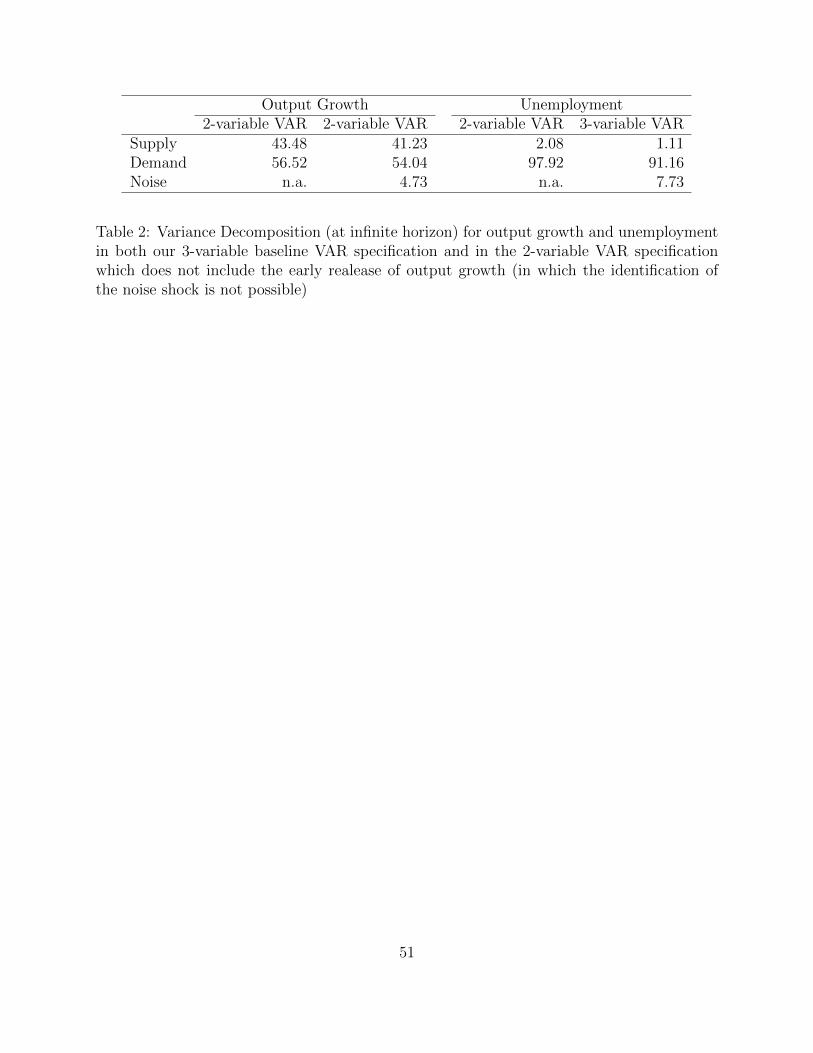
Output Growth Unemployment2-variable VAR 2-variable VAR 2-variable VAR 3-variable VAR

Supply 43.48 41.23 2.08 1.11Demand 56.52 54.04 97.92 91.16Noise n.a. 4.73 n.a. 7.73

Table 2: Variance Decomposition (at infinite horizon) for output growth and unemploymentin both our 3-variable baseline VAR specification and in the 2-variable VAR specificationwhich does not include the early realease of output growth (in which the identification ofthe noise shock is not possible)

51