UNCERTAINTY SHOCKS ARE AGGREGATE DEMAND SHOCKS

SYLVAIN LEDUC AND ZHENG LIU

Abstract. We present empirical evidence and a theoretical argument that uncertainty

shocks act like a negative aggregate demand shock, which raises unemployment and lowers

inflation. We measure uncertainty using survey data from the United States and the United

Kingdom. We estimate the macroeconomic effects of uncertainty shocks in a vector autore-

gression (VAR) model, exploiting the relative timing of the surveys and macroeconomic data

releases for identification. Our estimation reveals that uncertainty shocks accounted for at

least one percentage point increases in unemployment in the Great Recession and recovery,

but did not contribute much to the 1981-82 recession. We present a DSGE model to show

that, to understand the observed macroeconomic effects of uncertainty shocks, it is essential

to have both labor search frictions and nominal rigidities.

I. Introduction

Since the Great Recession, there has been a rapidly growing strand of literature—led by

the influential work of Bloom (2009)—that studies the macroeconomic effects of uncertainty

shocks. Most of the studies focus on the effects of uncertainty on real economic activity such

as investment and output. Less is known about the joint effects of uncertainty on inflation

and unemployment, and thus about the role of monetary policy in an environment with

heightened uncertainty.

In this paper, we provide some empirical evidence and a theoretical argument that uncer-

tainty shocks consistently act like aggregate demand shocks, which raise unemployment and

Date: June 19, 2013.

Key words and phrases. Uncertainty, Demand shocks, Unemployment, Inflation, Monetary policy, Survey

data.

JEL classification: E21, E27, E32.

Leduc: Federal Reserve Bank of San Francisco; Email: Sylvain.Leduc@sf.frb.org. Liu: Federal Reserve

Bank of San Francisco; Email: Zheng.Liu@sf.frb.org. We thank Susanto Basu, Nick Bloom, Toni Braun,

Mary Daly, John Fernald, Jesus Fernandez-Villaverde, Cristina Fuentes-Albero, Simon Gilchrist, Bart Hob-

jin, Giorgio Primiceri, Federico Ravenna, Juan F. Rubio-Ramırez, Pedro Silos, Pengfei Wang, John Williams,

Tao Zha and seminar participants at the Federal Reserve Banks of Atlanta and San Francisco, the Bank

of Canada, the Canadian Macro Study Group, the 2012 NBER Productivity and Macroeconomics meeting,

and the 2012 NBER Workshop on Methods and Applications for Dynamic Stochastic General Equilibrium

Models. We are grateful to Tao Zha for providing us with his computer code for estimating Bayesian VAR

models. The views expressed herein are those of the authors and do not necessarily reflect the views of the

Federal Reserve Bank of San Francisco or the Federal Reserve System.1

UNCERTAINTY SHOCKS ARE AGGREGATE DEMAND SHOCKS 2

lower inflation. Since both inflation and economic activity declines, policymakers react to

an increase in uncertainty by lowering the nominal interest rate both in our model and in

the data.

Despite the importance attached to uncertainty shocks, formal empirical studies on how

uncertainty shocks impact upon macroeconomic fluctuations remain scant. To fill this gap in

the literature, we provide evidence on the effects of uncertainty shocks on the macro economy,

using direct measures of perceived uncertainty by consumers and firms from survey data in

vector-autoregression (VAR) models.

Specifically, we construct measures of uncertainty using data from the University of Michi-

gan Survey of Consumers in the United States and the Confederation of British Industry

(CBI) Industrial Trends Survey of firms in the United Kingdom. Both surveys tally re-

sponses that make explicit references to “uncertainty” in affecting consumers’ decisions to

buy durable goods such as cars in the U.S. or firms’ decisions on capital expenditures in

the U.K.. We exploit the timing of the surveys’ construction to help identify structural

shocks to uncertainty. We examine their effects on three macroeconomic time series: the

unemployment rate, the CPI inflation rate, and the three-month T-bill rate.

A robust result that emerges from our study is that an increase in uncertainty raises

unemployment and lowers inflation and short-term nominal interest rates. The negative co-

movement between the responses of unemployment and inflation suggests that uncertainty

acts like a negative aggregate demand shock, for which policymakers accommodate by low-

ering the nominal interest rate. This pattern occurs in both the United States and in the

United Kingdom. It holds for different identification strategies. It also holds for a few al-

ternative measures of uncertainty, including the VIX index studied by Bloom (2009) and

the policy uncertainty index proposed by Baker, Bloom, and Davis (2011). We show that

the results are robust to controlling for movements in consumer confidence, expected future

income, or credit spreads, variables that can potentially mitigate the effects of uncertainty

shocks empirically (see, for instance, Gilchrist et al (2010) and Baker, Bloom, and Davis

(2011)).

We also find evidence that uncertainty can deepen recessions and hinder recoveries in

quantitatively important ways. In our benchmark VAR model with the household-survey

based measure of perceived uncertainty, uncertainty shocks account for at least one per-

centage point increase in the unemployment rate from the fall of 2008 through the end of

our sample in the first half of 2012. Our survey-based measure of uncertainty is broad and

does not isolate a particular source of uncertainty. When we use a finer measure of un-

certainty related to economic policy proposed by Baker, Bloom, and Davis (2011), we find

UNCERTAINTY SHOCKS ARE AGGREGATE DEMAND SHOCKS 3

that uncertainty shocks continue to be an important factor explaining the sharp increase in

unemployment in the Great Recession and recovery.

Interestingly, uncertainty shocks did not always play an important role during previous

recessions and recoveries. For example, uncertainty shocks contributed very little to the

sharp increase in unemployment during the 1981-82 recession. This latter finding accords

well with the view that monetary policy tightening under Fed Chairman Paul Volcker may

have played a more important role in that recession.

To help understand the mechanisms through which uncertainty shocks can be propagated

to generate the observed demand-shock like effects in the macroeconomy, we study a dynamic

stochastic general equilibrium (DSGE) model that incorporates labor search frictions and

nominal rigidities. Incorporating labor market frictions in the DSGE model enables us to

examine the effects of uncertainty shocks on unemployment explicitly. More importantly, we

show that uncertainty shocks can be substantially amplified through interactions between

search frictions and nominal rigidities.

The model economy is populated by a large number of identical and infinitely lived house-

holds. The representative household is a family of workers, some are employed and the others

are not. In each period, unemployed workers search for jobs and firms post vacancies at a

fixed cost, with a matching technology transforming searching workers and vacancies into

new job matches. When a match is formed, a wage is determined from a Nash bargaining

game between the new firm and the household. In each period, a fraction of employed work-

ers is separated exogenously from their matches. Thus, aggregate employment in a given

period is the sum of the number of workers that survive separation and the number of new

matches formed.1

To introduce nominal rigidities, we follow Blanchard and Galı (2010) and assume that

there is a retail sector, in which a large number of retailers produce differentiated retail

products using the homogenous intermediate good produced by firms as input. While the

intermediate good market is perfectly competitive, the retail goods market is monopolistically

competitive. The final consumption good is a Dixit-Stiglitz composite of the differentiated

retail products. Each retailer sets a price for its own product subject to a price adjustment

cost (Rotemberg, 1982). The retailer takes the price index and the demand schedule for its

product as given. Monetary policy follows a feedback interest rate rule (i.e., a Taylor rule),

under which the nominal interest rate reacts to deviations of inflation from a target and also

to fluctuations in output gap.

1The type of search friction that we consider here takes its root from the original contributions by Diamond

(1982) and Mortensen and Pissarides (1994).

UNCERTAINTY SHOCKS ARE AGGREGATE DEMAND SHOCKS 4

Since the demand-shock like effects of uncertainty shocks hold for a broad set of measures of

uncertainty in our empirical work, we consider three types of uncertainty in our model related

to preferences, technology, and fiscal policy. We find that, consistent with our empirical

results, a rise in uncertainty—regardless of its source—is always contractionary and always

lowers inflation. Under the Taylor rule, the monetary authority reacts to the declines in

output and inflation by lowering the nominal interest rate.

Our model suggests that labor search frictions and nominal rigidities are both important

for amplifying the macroeconomic effects of uncertainty shocks. For example, absent nominal

rigidities, a technology uncertainty shock generates a response of unemployment that is about

one sixth as large as that in our benchmark model. Similarly, absent significant search

frictions, the effects of a technology uncertainty shock on unemployment is about one third

as large as in the benchmark model.

Nominal rigidities help amplify the effect of uncertainty shocks in a DSGE model through

variations in markups (Fernandez-Villaverde, Guerron-Quintana, Kuester, and Rubio-Ramırez,

2011; Basu and Bundick, 2011). With sticky prices, an uncertainty shock that lowers aggre-

gate demand also lowers the relative price of intermediate goods, which corresponds to the

inverse of the markup in the retail sector. The decline in the relative price reduces the value

of a new match, so that firms post fewer job vacancies and the unemployment rate rises.

As more searching workers fail to find a job match, the household’s income declines further,

leading to an even greater fall in aggregate demand, which reinforces the initial decline in the

relative price, creating a multiplier effect that amplifies uncertainty shocks to generate large

macroeconomic fluctuations. This amplification mechanism is absent in the flexible-price

model, since the relative price is constant.

Search frictions in the labor market provide an additional mechanism for uncertainty

shocks to generate large increases in unemployment. This mechanism reflects the impact

of uncertainty shocks on the value of a job match and the shape of the Beveridge curve,

which captures the negative and convex relationship between vacancies and unemployment.

When the cost of posting a vacancy is very low, which would approximate a frictionless labor

market, equilibrium unemployment is determined along a relatively inelastic segment of the

Beveridge curve. In this case, a rise in uncertainty lowers the value of a filled vacancy; but

for any given decline in posted vacancies, the increase in unemployment is muted. However,

when the cost of posting vacancies is high (i.e., when search frictions are more important),

a given decline in posted vacancies would be associated with a much larger increase in un-

employment, since equilibrium unemployment is determined along a relatively more elastic

segment of the Beveridge curve. Thus, in our model, search frictions have important inter-

actions with sticky prices to amplify uncertainty shocks.

UNCERTAINTY SHOCKS ARE AGGREGATE DEMAND SHOCKS 5

Our work adds to the recent rapidly growing literature that studies the macroeconomic ef-

fects of uncertainty shocks in a DSGE framework. For example, Bloom, Floetotto, Jaimovich,

Saporta-Eksten, and Terry (2012) study a DSGE model with heterogeneous firms and non-

convex adjustment costs in productive inputs. They find that a rise in uncertainty makes

firms pause hiring and investment and thus leads to a large drop in economic activity. Chris-

tiano, Motto, and Rostagno (2012) present a DSGE model with a financial accelerator in the

spirit of Bernanke, Gertler, and Gilchrist (1999). They find that risk shocks (i.e., changes in

the volatility of cross-sectional idiosyncratic uncertainty) play an important role for shaping

U.S. business cycles. Barro (2006) shows that rare disasters—a form of risk shocks—help rec-

oncile some asset pricing puzzles in business cycle models (see also Gabaix (2012) and Gourio

(2012)). Gilchrist, Sim, and Zakrajsek (2010) and Arellano, Bai, and Kehoe (2011) argue

that uncertainty shocks have important interactions with financial factors. Related to the

general issue of uncertainty and risks, Ilut and Schneider (2011) examine the macroeconomic

implications of ambiguity aversion in an estimated medium-scale DSGE model.2

Our work is closely related to Fernandez-Villaverde, Guerron-Quintana, Kuester, and

Rubio-Ramırez (2011), who examine the effects of fiscal policy uncertainty and find that

it can trigger sizable adverse effects on economic activity in a model with price and wage

rigidities, particularly in the case of uncertainty about taxes on capital income. Our work is

also closely related to the study by Basu and Bundick (2011), who focus on the importance

of nominal rigidities to generate comovement between macroeconomic variables following an

uncertainty shock. We share a similar emphasis with these studies that uncertainty shocks

work through an aggregate demand channel in the presence of nominal rigidities. We further

point out that the macroeconomic effects of uncertainty can be substantially amplified by

search frictions in the labor market. This point, to our knowledge, is new to the literature.

Most of the studies in the literature abstract from labor search frictions and are not

designed to examine the impact of uncertainty shocks on labor market dynamics such as

unemployment and job vacancies. An exception is Schaal (2012), who presents a model with

labor search frictions and idiosyncratic volatility shocks to study the observation in the Great

Recession period that high unemployment was accompanied by high labor productivity. As

2The literature suggests that rising uncertainty may hinder irreversible investment and hiring decisions,

because it raises the option value of waiting. For partial equilibrium analyses of the real option value theory

in the context of uncertainty shocks, see, for example, (Bernanke, 1983) and Bloom (2009). Romer (1990)

argues that increases in uncertainty following the stock market crash in 1929 contributed to worsening the

Great Depression by substantially reducing demand for consumer durable goods. For empirical evidence on

the effects of uncertainty on investment, see, for example, Leahy and Whited (1996) and Guiso and Parigi

(1999). For a comprehensive survey of the literature on uncertainty shocks, see Bloom and Fernandez-

Villaverde (2012).

UNCERTAINTY SHOCKS ARE AGGREGATE DEMAND SHOCKS 6

in the other studies discussed here, he focuses on the effects of uncertainty on real activity,

not on its interaction with inflation and monetary policy. In addition, he assumes that

uncertainty shocks are negatively correlated with aggregate productivity, so that such shocks

can have important recessionary effects. In our model, we do not assume correlations between

uncertainty shocks and the level of aggregate productivity; instead, uncertainty shocks are

amplified through interactions between nominal rigidities and labor search frictions.

In what follows, we present in Section II empirical evidence that uncertainty shocks con-

sistently act like an aggregate demand shock. We then present in Section III a DSGE model

with labor search frictions and sticky prices. We discuss in Section IV the dynamic effects of

uncertainty shocks on unemployment and other macroeconomic variables in the calibrated

DSGE model. We provide some concluding remarks in Section V.

II. The Macroeconomic Effects of Uncertainty Shocks: Evidence

In this section, we examine the macroeconomic effects of uncertainty shocks in the data.

We first present two new measures of uncertainty from survey data. We then estimate a

VAR model that includes a measure of uncertainty and a few macroeconomic variables.

VAR models are used in the literature as a main statistical tool to estimate the responses of

macroeconomic variables to uncertainty shocks. Examples include Alexopoulos and Cohen

(2009), Bloom (2009), Bachmann, Elstner, and Sims (2011), and Baker, Bloom, and Davis

(2011). Existing studies focus on the effects of uncertainty on real economic activity such

as employment, investment, and output. We focus on the joint effects of uncertainty on

unemployment and inflation.

II.1. Measures of uncertainty. We consider two new measures of uncertainty from survey

data, including a measure of perceived uncertainty by consumers from the Michigan Survey of

Consumers and a measure of perceived uncertainty by firms from the CBI Industrial Trends

Survey in the United Kingdom. Since these two survey-based measures of uncertainty are

new in the literature, we begin with some explanations of how these measures are constructed

in the survey.

Each month since 1978, the Michigan Survey has been conducting interviews of about 500

households throughout the United States, asking questions ranging from their perceptions of

business conditions to expectations for future movements in prices. More important for our

analysis, the survey tallies the fraction of respondents who report that “uncertain future”is

a factor that will likely limit their expenditures on cars or other durable goods over the next

12 months.3

3The question on vehicle purchases is, “Speaking now of the automobile market–do you think the next 12

months or so will be a good time or a bad time to buy a vehicle, such as a car, pickup, van or sport utility

UNCERTAINTY SHOCKS ARE AGGREGATE DEMAND SHOCKS 7

Figure 1 shows the time-series plots of consumers’ perceived uncertainty (concerning ve-

hicle purchases) along with the VIX index—a commonly used measure of uncertainty in

the literature (Bloom, 2009). Similar to the VIX index, consumers’ perceived uncertainty is

countercyclical. It rises in recessions and falls in expansions. A notable difference between

the consumers’ perceived uncertainty and financial uncertainty measured by the VIX is that

the 1997 East-Asian financial crisis and the 1998 Russian debt crisis led to large spikes in

the VIX, but did not seem to have much impact on consumer perceptions of uncertainty.

Another notable difference is that, in the more recent months in 2012, the VIX index has

stayed at low levels despite of the looming “fiscal cliff” that would trigger large increases in

taxes and substantial cuts in government spending if the Congress and the White House can-

not reach an agreement for deficit cuts. However, consumer uncertainty from the Michigan

survey has remained elevated during this period.4

We follow a similar procedure to construct firms perceived uncertainty from the CBI

Industrial Trends Survey in the United Kingdom. Each quarter since 1978, the CBI has

been surveying a large sample of roughly 1,100 firms in the United Kingdom in each quarter.

We measure firms’ perceived uncertainty as the fraction of firms that report “uncertainty

about demand” as a factor limiting their capital expenditures over the next 12 months.5

As Figure 2 shows, firms’ perceived uncertainty is also countercyclical, but it appears

relatively more stable than what is reported by the Michigan survey of consumers. This

difference may reflect the fact that U.K. firms are asked about a specific form of uncertainty

(i.e., about the demand for their products), whereas no such specificity is attached to the

measure of uncertainty in the Michigan survey.

II.2. Empirical results. We now examine the macroeconomic effects of uncertainty shocks

by estimating a Baysian vector autoregression (BVAR) model. Sims and Zha (1998) argue

that sampling errors can lead to difficulties in estimating error bands for impulse responses

in a VAR model with a short time-series sample of data. They propose using Baysian

priors (instead of flat priors) to help improve the estimation of error bands. We follow their

approach in our analysis.

In our benchmark VAR model, we consider four variables, including a measure of uncer-

tainty, the unemployment rate, the inflation rate measured as the year-over-year change in

vehicle? Why do you say so?” Reasons related to uncertainty are then compiled. The series is weighted by

age, income, region, and sex to be nationally representative.4A possible explanation is that the VIX index focuses on short-term uncertainty because it is a weighted

average of 30-day ahead option prices.5The question asked by the CBI is, “What factors are likely to limit (wholly or partly) your capital expen-

diture authorisations over the next twelve months?” Participants can choose “uncertainty about demand”

as one of six options. Firms can provide other reasons or choose multiple reasons.

UNCERTAINTY SHOCKS ARE AGGREGATE DEMAND SHOCKS 8

the consumer price index (CPI), and the three-month Treasury bills rate. The sample ranges

from January 1978 to November 2012.

In our benchmark VAR model, we exploit the timing of survey interviews relative to the

timing of macroeconomic data releases for identification. To examine the robustness of our

results, we also consider alternative identification schemes in Section II.4.2. In the Michigan

survey, phone interviews are conducted throughout the month, with most interviews con-

centrated in the middle of each month, and preliminary results released shortly thereafter.

The final results are typically released by the end of the month. When answering questions,

survey participants have information about the previous month’s unemployment, inflation,

and interest rates, but they do not have (complete) information about the current-month

macroeconomic conditions because the macroeconomic date have not yet been made public.

Hence, our identification strategy uses the fact that when answering questions at time t about

their expectations of the future, the information set on which survey participants condition

their answers will not include, by construction, the time t realizations of the unemployment

rate and the other variables in our VAR.6 Thus, we follow the approach in Leduc, Sill, and

Stark (2007), Auerbach and Gorodnichenko (2012), and Leduc and Sill (forthcoming) by

placing the uncertainty measure as the first variable in the VAR. This Cholesky ordering im-

plies that uncertainty does not respond to macroeconomic shocks in the impact period, while

unemployment, inflation, and the nominal interest rate are allowed to change on impact of

an uncertainty shock.7

We first look at the transmission of uncertainty shocks in the Unites States using the

measure of consumer uncertainty from the Michigan Survey. Figure 3 presents the impulse

responses in the VAR model, in which consumer uncertainty is ordered first. For each

variable, the solid line denotes the median estimate of the impulse response and the dashed

lines represent the range of the 90-percent confidence band around the point estimates. The

figure shows that an unexpected increase in uncertainty leads to a persistent increase in the

unemployment rate, which reaches a peak in about 18 months from the impact period and

remains significantly positive for about three years. Heightened uncertainty also leads to a

6Similarly, the questionnaires for the CBI survey must be returned by the middle of the first month of

each quarter. The design of the survey implies that participants have information about the values of the

variables in the VAR for the previous quarter when they filled in answers to the survey questions, but they

do not know the macroeconomic data in the current quarter.7Bachmann and Moscarini (2011) argue that bad first-moment shocks can raise cross-sectional disper-

sions and time-series volatility of macroeconomic variables. In this sense, changes in measured uncertainty

could reflect endogenous responses of macroeconomic variables to first-moment shocks. Our empirical ap-

proach allows measured uncertainty to react to macroeconomic shocks, but it also presumes that measured

uncertainty contains some exogenous component.

UNCERTAINTY SHOCKS ARE AGGREGATE DEMAND SHOCKS 9

significant and persistent decline in inflation, with the peak effect also occurring roughly 18

months after the shock.

The aggregate demand effect of uncertainty is not unique to the U.S. economy. It is also

present in the U.K. data. Using the measure of firms’ perceived uncertainty from the CBI

Survey, we examine the effects of uncertainty shocks in a VAR model using UK data on

unemployment, inflation, and the three-month nominal interest rate. Since the survey data

are quarterly, we convert the unemployment rate, the inflation rate, and the 3-month nominal

interest rate from monthly to quarterly frequency by taking the end of quarter observations

(e.g., unemployment for the first quarter of 1980 is the unemployment rate in March 1980

and for the second quarter, it is that in June, and so on). The sample ranges from 1979:Q4

to 2011:Q2. Figure 4 shows that an unanticipated increase in the level of uncertainty leads

to persistent increases in unemployment and persistent declines in both the inflation rate

and the nominal interest rate in the U.K. sample, just as those observed in the U.S. data.

II.3. Quantitative importance of uncertainty shocks. How important are uncertainty

shocks for macroeconomic fluctuations? This question is important, especially in light of the

recent discussions about potential consequences of going over the fiscal cliff for the United

States economy. We have seen that the estimated impulse responses of unemployment to

an uncertainty shock are statistically significant. Those impulse responses, however, reflect

the average effects of an increase in uncertainty on unemployment in the entire sample; they

do not indicate the relative importance of uncertainty shocks for unemployment in different

recessions. Our sample of U.S. data covers 4 different recessions, with particularly large

increases in unemployment in 2 of them: one in the early 1980s and the other during the

Great Recession and recovery periods since 2008. We focus on these 2 recessions and ask the

question: How much of the observed increases in unemployment in each of these recessions

are accounted for by increases in the levels of uncertainty?

To provide an answer to this question, we calculate historical decompositions from our

estimated VAR model. This calculation is a counterfactual experiment. By construction,

if we have all 4 shocks turned on in our benchmark 4-variable VAR model, the estimated

VAR model would exactly match the observed time series of the unemployment rate. The

counterfactual experiment that we conduct is one in which we turn off all shocks but the

uncertainty shock in the VAR model and calculate the implied unemployment path in each

of the two recession periods.

Figure 5 shows the changes in the unemployment rate during the Great Recession and

recovery period (the top panel) and those in the 1981-82 recession (the bottom panel).

The thin blue lines indicate the actual increases in the unemployment rate (relative to the

benchmark with no shocks) in each of the two recessions; the red bars indicate the simulated

UNCERTAINTY SHOCKS ARE AGGREGATE DEMAND SHOCKS 10

unemployment rate when all 4 shocks are turned on (and, by construction, they match the

actual data exactly); and the blue bars indicate the simulated changes in the unemployment

rate conditional on the estimated uncertainty shocks alone.

The figure reveals that uncertainty shocks have contributed about 30-40% of the actual

increases in the unemployment rate in the Great Recession and recovery. In particular, out

of the 3-4 percentage point increases in unemployment from 2008 through the end of our

sample in 2012, about 1-1.5 percentage points are accounted for by heightened uncertainty.

A possible reason why uncertainty shocks contributed to large increases in unemployment

in the Great Recession and recovery is that monetary policy has been constrained by the

zero lower bound on the nominal interest rate during this period. This view is consistent

with Basu and Bundick (2011), who find that, in a calibrated DSGE model, the adverse

effects of uncertainty shocks on aggregate output are substantially amplified when the policy

rate reaches the zero lower bound.

In contrast, uncertainty shocks contributed little to the surge in unemployment during

the 1981-82 recession period. This latter finding is consistent with the view that monetary

policy tightening under Fed Chairman Paul Volcker was an important driving force of the

recession in the early 1980s.8

II.4. Robustness. The finding that uncertainty shocks act like aggregate demand shocks is

fairly robust. As we have just demonstrated, it holds for data in both the United States and

the United Kingdom, with two different measures of uncertainty (one reflects consumers’

perceptions of uncertainty in the U.S. and the other captures firms’ perceptions in the U.K.)

that display relatively different time-series properties. We now show that the results are also

robust to alternative measures of uncertainty, alternative identification assumptions, and

inclusions of additional macroeconomic variables in the VAR model.

II.4.1. Alternative measures of uncertainty. There are a few other measures of uncertainty

used in the literature. We focus on two particular measures, including the VIX index that

captures the stock price volatility, which, as shown by Bloom (2009), leads to substantial

declines in industrial output and employment in the short run; and the economic policy

uncertainty index constructed by Baker, Bloom, and Davis (2011), who show that a shock

to policy uncertainty foreshadows large declines in industrial output and employment.

8Similarly, uncertainty shocks did not contribute much to unemployment in the 2001 recession. However,

we do find that uncertainty shocks played a major role during and following the 1990-1991 recession. One

possibility is that this recession involved a military conflict in the Middle East, which might have ignited

fears of potentially catastrophic events such as disruptions of oil supply. Since the increases in unemployment

in these two episodes of recession were relatively small, we focus on the quantitative effects of uncertainty

on unemployment in the Great Recession and the 1981-82 recession.

UNCERTAINTY SHOCKS ARE AGGREGATE DEMAND SHOCKS 11

Our sample size depends on the measure of uncertainty. The VIX index constructed by

the Chicago Board of Exchange (CBOE) has a sample that starts in January 1990. We

extend the series back in time (for the pre-1990 periods) using the CBOE’s VXO index,

which starts in January 1986. The policy uncertainty index is a monthly series that starts

in January 1985. The ending period for both these uncertainty measures is November 2012.

Figure 6 shows that, when the uncertainty measure in our benchmark model is replaced

by the VIX index, an uncertainty shock raises unemployment and lowers inflation and the

nominal interest rate, just as what we observe when we use the survey-based measure of

uncertainty. Similarly, when we use the economic policy uncertainty index constructed by

Baker, Bloom, and Davis (2011), we obtain qualitatively identical results (see Figure 7). In

both cases, the responses of macroeconomic variables are statistically significant at the 90

percent level. Thus, our finding that an uncertainty shock acts like a negative aggregate

demand shock is robust to these alternative measures of uncertainty.

II.4.2. Alternative identification approaches. We now examine the sensitivity of our results

to alternative identification assumptions.

Although the timing of the survey relative to macroeconomic data releases suggests that

survey respondents do not possess complete information about the current-month macroe-

conomic data at the time of the interviews (which substantiates our Cholesky identification

assumption in the benchmark VAR model), it is possible that they observe other, possibly

higher-frequency variables that give them information about the time t realizations of the

variables in the VAR model. We thus estimate a VAR model with uncertainty ordered last.

This relatively conservative identification assumption implies that the measure of uncertainty

is allowed to respond to contemporaneous macroeconomic shocks.

Figure 8 presents the impulse responses in the VAR model with consumer uncertainty

(from the Michigan Survey) ordered last. The responses of the three macroeconomic vari-

ables to an uncertainty shock look remarkably similar to those in the baseline VAR with

uncertainty ordered first. Under each identification strategy, a positive uncertainty shock

acts like a negative aggregate demand shock that raises unemployment and lowers inflation.

In response to the recessionary effects of uncertainty shocks, monetary policy reacts by easing

the stance of policy and lowering the nominal interest rate.

To further examine the sensitivity of our results to the identification assumptions, we

estimate a VAR model with uncertainty measured by a dummy variable that takes a value

of one if there is an uncertainty event in a particular month and zero otherwise, where most

of the uncertainty events are identified by Bloom (2009).9 In estimating this VAR model, we

9Bloom (2009) identifies 17 uncertainty events for the periods from 1962 to 2008. To be consistent with

our benchmark VAR model, we focus on the sample from January 1978 to November 2012. Our sample

UNCERTAINTY SHOCKS ARE AGGREGATE DEMAND SHOCKS 12

follow Bloom (2009) and treat the uncertainty dummy as an exogenous variable, which does

not respond to changes in macroeconomic conditions. Figure 9 shows the impulse responses

of the macroeconomic variables following a shock to the uncertainty dummy. The figure

shows that an uncertainty shock leads to significant short-run increases in unemployment and

significant declines in inflation and the nominal interest rate, although the macroeconomic

responses are less persistent than those estimated from our benchmark VAR model with

consumer uncertainty. This finding lends further support to our view that uncertainty shock

acts like an aggregate demand shock.

II.4.3. Larger VAR models. To further examine the robustness of our results, we estimate

a few alternative VAR models that include additional macroeconomic variables. For ease

of comparison, we use consumers’ perceived uncertainty from the University of Michigan

survey in each model and we impose the same Cholesky identification restrictions as in our

benchmark model by ordering uncertainty first in these alternative VAR models.

One such larger VAR model includes, in addition to the 3 macroeconomic time series, a

measure of labor market tightness (measured by the ratio of the job vacancy rate to the

unemployment rate, or the v-u ratio). We measure job vacancies using data from JOLTS

combined with the Help-Wanted Index published by the Conference Board. The sample

range is the same as in our benchmark VAR model (from January 1978 to November 2012).

Figure 10 shows that an unexpected rise in uncertainty leads to a significant and persistent

increase in the unemployment rate and persistent declines in the v-u ratio. As in the bench-

mark model, the shock also lowers both the inflation rate and the nominal interest rate.

These observations, as we show in the theory section, are consistent with a DSGE model

with nominal rigidities and search frictions in the labor market. An uncertainty shock in this

larger VAR model continues to have macroeconomic effects that are similar to a negative

aggregate demand shock.

We have estimated other models that, in addition to the four variables in our baseline VAR

model (with consumer uncertainty ordered first), also include (i) consumption of nondurables

and services and business fixed investment; (ii) credit spread and stock price index; or (iii)

full-time and part-time employment. We have also estimated the baseline four-variable VAR

model with the sample ending at the end of 2008, before the policy rates in the United States

includes 11 uncertainty events taken from Bloom (2009) for the period between 1978 and 2008 (see his Table

A.1). We extend the sample to include a new uncertainty event that occurred in August 2011, when the

debt ceiling dispute triggered a downgrade of the United States government debt.

UNCERTAINTY SHOCKS ARE AGGREGATE DEMAND SHOCKS 13

and the United Kingdom hit the zero lower bound. In each case, uncertainty shocks con-

sistently act like an aggregate demand shock that raises unemployment and lowers inflation

and the nominal interest rate.10

II.5. Uncertain future or bad economic times? As shown in Figure 1, consumer uncer-

tainty rises in recessions and falls in booms. A priori, it is possible that consumer uncertainty

from the Michigan survey may reflect the respondents’ perceptions of “bad economic times”

rather than “uncertain future.”

To examine to what extent consumer uncertainty might reflect their perceptions of bad

economic times, we examine to what extent the macroeconomic effects of shocks to consumer

uncertainty may reflect the responses to changes in other indicators of economic conditions,

such as consumer confidence. For this purpose, we follow a similar approach in Baker, Bloom,

and Davis (2011) and estimate a 5-variable VAR model that includes a consumer sentiment

index as an additional variable to control for potential effects from movements in consumer

confidence.

Figure 11 shows that the macroeconomic effects of uncertainty shocks are qualitatively

similar to those estimated from the benchmark VAR. Following an exogenous increase in

uncertainty, consumer sentiment declines, unemployment rises, and inflation and the nom-

inal interest rate both fall. The responses of the macroeconomic variables are statistically

significant at the 90 percent level. Thus, the macroeconomic effects of consumer uncertainty

shocks do not seem to reflect responses of macroeconomic variables to changes in consumer

confidence.11

III. Uncertainty shocks in a DSGE model with search frictions

In this section, we examine the channels of transmission for uncertainty shocks to affect

the macroeconomy in a DSGE model with sticky prices and labor market search frictions.

We show that uncertainty shocks in the DSGE model act like an aggregate demand shock

that raises unemployment, lowers inflation, and through the Taylor rule, lowers the nominal

interest rate, just as what we have seen in the data. We further show that search frictions

in the labor market and sticky prices in the goods market are both important for amplifying

the effects of uncertainty shocks in the model.

10To conserve space, we do not report the impulse response figures in the paper. These figures are included

in a supplemental appendix.11The consumer sentiment index that we use here is a measure of consumer sentiment about current

economic conditions. We have also estimate a 5-variable VAR model by using the consumer sentiment index

for expectations. The qualitative results are also very similar to those in the benchmark VAR model.

UNCERTAINTY SHOCKS ARE AGGREGATE DEMAND SHOCKS 14

The model builds on the basic framework in Blanchard and Galı (2010), generalized to

incorporate capital accumulations. The model is similar to that presented in Liu, Miao,

and Zha (2013), who study the interactions between housing prices and unemployment.

The difference is that we focus on the aggregate demand effects of uncertainty shocks by

incorporating sticky prices.

The economy is populated by a continuum of infinitely lived and identical households with

a unit measure. The representative household consists of a continuum of worker members.

The household owns a continuum of firms, each of which uses one worker, along with capital

inputs, to produce an intermediate good. In each period, a fraction of the workers are

unemployed and they search for a job. Firms post vacancies at a fixed cost. The number

of successful matches are produced with a matching technology that transforms searching

workers and vacancies into an employment relation. Real wages are determined by Nash

bargaining between a searching worker and a hiring firm.

The household consumes and invests a basket of differentiated retail goods, each of which

is transformed from the homogeneous intermediate good using a constant-returns technology.

Retailers face a perfectly competitive input market (where they purchase the intermediate

good) and a monopolistically competitive product market. Each retailer sets a price for its

differentiated product, with price adjustments subject to a quadratic cost in the spirit of

Rotemberg (1982).

The government finances its spending and transfer payments to unemployed workers by

distortionary taxes on firm profits. Monetary policy is described by the Taylor rule, under

which the nominal interest rate responds to deviations of inflation from a target and of

output from its potential.

III.1. The households. There is a continuum of infinitely lived and identical households

with a unit measure. The representative household consumes and invests a basket of retail

goods. The utility function is given by

E∞∑t=0

βtAt (ln(Ct − bCt−1)− χNt) , (1)

where E [·] is an expectation operator, Ct denotes consumption, Nt denotes the fraction of

household members who are employed, β ∈ (0, 1) denotes the subjective discount factor,

b ∈ (0, 1) is a habit-persistence parameter, and χ measures the disutility from working.

The term At denotes an intertemporal preference shock. Let γat ≡ AtAt−1

denote the growth

rate of At. We assume that γat follows the stochastic process

ln γat = ρa ln γa,t−1 + σatεat. (2)

UNCERTAINTY SHOCKS ARE AGGREGATE DEMAND SHOCKS 15

The parameter ρa ∈ (−1, 1) measures the persistence of the preference shock. The term εat

is an i.i.d. standard normal process. The term σat is a time-varying standard deviation of

the innovation to the preference shock. We interpret it as a preference uncertainty shock.

We assume that σat follows the stationary process

lnσat = (1− ρσa) lnσa + ρσa lnσa,t−1 + σσaεσa,t, (3)

where ρσa ∈ (−1, 1) measures the persistence of preference uncertainty, εσa,t denotes the

innovation to the preference uncertainty shock and is a standard normal process, and σσa

denotes the (constant) standard deviation of the innovation.

The representative household is a family consisting of a continuum of workers with a

unit measure. The family chooses consumption Ct, investment It, saving Bt, and capacity

utilization rate et to maximize the utility function in (1) subject to the sequence of budget

constraints

Ct + It +Bt

PtRt

=Bt−1

Pt+ wtNt + φ (1−Nt) + [rktet − Φ(et)]Kt−1 + Πt, ∀t ≥ 0, (4)

where Pt denotes the price level, Bt denotes the household’s holdings of a nominal risk-free

bond, Rt denotes the nominal interest rate, wt denotes the real wage rate, φ denotes an

unemployment benefit, rkt denotes the capital rental rate, and Πt denotes profit income

from the household’s ownership of intermediate goods producers and of retailers.

The term Φ(et) represents a cost function for capacity utilization. We assume that the

function takes the form

Φ(et) = φ1(et − e) +φ2

2(et − e)2, (5)

where φ1 measures the slope and φ2 measures the curvature of the utilization cost function.

The constant e denotes the steady-state capacity utilization rate, which we normalize to one.

The stock of capital evolves according to the law of motion

Kt = (1− δ)Kt−1 +

[1− ΩI

2

(ItIt−1− γI

)2]It, (6)

where δ ∈ (0, 1) denotes the capital depreciation rate, ΩI ∈ (0,∞) measures the scale of

investment adjustment costs, and γI is the steady-state growth rate of investment.

UNCERTAINTY SHOCKS ARE AGGREGATE DEMAND SHOCKS 16

The first-order necessary conditions for the household’s optimizing decisions are summa-

rized in the following equations:

Λt =At

Ct − bCt−1− Et

βbAt+1

Ct+1 − bCt, (7)

1 = EtβΛt+1

Λt

Rt

πt+1

, (8)

Qkt = EtβΛt+1

Λt

[rk,t+1et+1 − Φ (et+1) + (1− δ)Qk,t+1] , (9)

1 = Qkt

[1− ΩI

2

(ItIt−1− γI

)2

− ΩI

(ItIt−1− γI

)ItIt−1

]

+ EtβΛt+1

Λt

Qkt+1ΩI

(It+1

It− γI

)(It+1

It

)2

, (10)

rkt = φ2 (et − 1) + φ1, (11)

III.2. The aggregation sector. Denote by Yt the final consumption good, which is a basket

of differentiated retail goods. Denote by Yt(j) a type j retail good for j ∈ [0, 1]. We assume

that

Yt =

(∫ 1

0

Yt(j)θ−1θ

) θθ−1

, (12)

where θ > 1 denotes the elasticity of substitution between differentiated products.

Expenditure minimizing implies that demand for a type j retail good is inversely related

to the relative price, with the demand schedule given by

Y dt (j) =

(Pt(j)

Pt

)−θYt, (13)

where Y dt (j) and Pt(j) denote the demand for and the price of retail good of type j, respec-

tively. The price index Pt is related to the individual prices Pt(j) through the relation

Pt =

(∫ 1

0

Pt(j)1

1−θ

)1−θ

. (14)

III.3. The retail goods producers. There is a continuum of retail goods producers, each

producing a differentiated product using a homogeneous intermediate good as input. The

production function of retail good of type j ∈ [0, 1] is given by

Yt(j) = Xt(j), (15)

where Xt(j) is the input of intermediate goods used by retailer j and Yt(j) is the output. The

retail goods producers are price takers in the input market and monopolistic competitors in

the product markets, where they set prices for their products, taking as given the demand

schedule in equation (13) and the price index in equation(14).

UNCERTAINTY SHOCKS ARE AGGREGATE DEMAND SHOCKS 17

Price adjustments are subject to the quadratic cost

Ωp

2

(Pt(j)

πPt−1(j)− 1

)2

Yt, (16)

where the parameter Ωp ≥ 0 measures the cost of price adjustments and π denotes the

steady-state inflation rate. Here, we assume that price adjustment costs are in units of

aggregate output.

A retail firm that produces good j solves the profit-maximizing problem

maxPt(j) Et

∞∑i=0

βiΛt+iAt+iΛtAt

[(Pt+i(j)

Pt+i− qt+i

)Y dt+i(j)−

Ωp

2

(Pt+i(j)

πPt+i−1(j)− 1

)2

Yt+i

],

(17)

where qt+i denotes the relative price of intermediate goods in period t + i. The optimal

price-setting decision implies that, in a symmetric equilibrium with Pt(j) = Pt for all j, we

have

qt =θ − 1

θ+

Ωp

θ

[πtπ

(πtπ− 1)− Et

βγa,t+1Λt+1

Λt

Yt+1

Yt

πt+1

π

(πt+1

π− 1)]

. (18)

Absent price adjustment costs (i.e., Ωp = 0), the optimal pricing rule implies that real

marginal cost qt equals the inverse of the steady-state markup.

III.4. The Labor Market. In the beginning of period t, there are ut unemployed workers

searching for jobs and there are vt vacancies posted by firms. The matching technology is

described by the Cobb-Douglas function

mt = µuat v1−at , (19)

where mt denotes the number of successful matches and the parameter a ∈ (0, 1) denotes

the elasticity of job matches with respect to the number of searching workers. The term µ

scales the matching efficiency.

The probability that an open vacancy is matched with a searching worker (or the job

filling rate) is given by

qvt =mt

vt. (20)

The probability that an unemployed and searching worker is matched with an open vacancy

(or the job finding rate) is given by

qut =mt

ut. (21)

In the beginning of period t, there are Nt−1 workers. A fraction ρ of these workers lose

their jobs. Thus, the number of workers who survive the job separation is (1 − ρ)Nt−1. At

the same time, mt new matches are formed. Following the timing assumption in Blanchard

UNCERTAINTY SHOCKS ARE AGGREGATE DEMAND SHOCKS 18

and Galı (2010), we assume that new hires start working in the period they are hired. Thus,

aggregate employment in period t evolves according to

Nt = (1− ρ)Nt−1 +mt. (22)

With a fraction ρ of employed workers separated from their jobs, the number of unemployed

workers searching for jobs in period t is given by

ut = 1− (1− ρ)Nt−1. (23)

Following Blanchard and Galı (2010), we assume full participation and define the unemploy-

ment rate as the fraction of the population who are left without a job after hiring takes place

in period t. Thus, the unemployment rate is given by

Ut = ut −mt = 1−Nt. (24)

III.5. The firms (intermediate good producers). A firm can produce only if it can

successfully match with a worker. A firm produce intermediate goods using a worker and

some capital inputs, with the production function

xt = Ztkαt ,

where xt is output, kt is capital input, and Zt is an aggregate technology shock. The

parameter α ∈ (0, 1) is the output elasticity of capital stock.

The technology shock follows the stochastic process

lnZt = (1− ρz) lnZ + ρz lnZt−1 + σztεzt. (25)

The parameter ρz ∈ (−1, 1) measures the persistence of the technology shock. The term εzt

is an i.i.d. innovation to the technology shock and is a standard normal process. The term

σzt is a time-varying standard deviation of the innovation and we interpret it as a technology

uncertainty shock. We assume that the technology uncertainty shock follows the stationary

stochastic process

lnσzt = (1− ρσz) lnσz + ρσz lnσz,t−1 + σσzεσz ,t, (26)

where the parameter ρσz ∈ (−1, 1) measures the persistence of the technology uncertainty,

the term εσz ,t denotes the innovation to the technology uncertainty and is a standard normal

process, and the parameter σσz > 0 is the standard deviation of the innovation.

If a firm finds a match, it obtains a flow profit in the current period after paying the

worker and capital rents. In the next period, if the match survives (with probability 1− ρ),

the firm continues; if the match breaks down (with probability ρ), the firm posts a new job

vacancy at a fixed cost κ, with the value Vt+1.

UNCERTAINTY SHOCKS ARE AGGREGATE DEMAND SHOCKS 19

The value of a firm with a match is given by the Bellman equation

JFt = (1− τt)(qtxt − rktkt − wt) + EtβΛt+1

Λt

[(1− ρ) JFt+1 + ρVt+1

], (27)

where τt denotes a tax rate on flow profits.

The firm’s optimal choice of capital input solves the problem

dt ≡ maxk

qtZtkα − rktk. (28)

The first order condition implies that

rkt = αqtxtkt

. (29)

The dividend (i.e., profit before wage payments) is given by

dt = (1− α)(qtZt)1

1−α

(α

rkt

) α1−α

. (30)

Thus, the firm’s flow dividend income is a function of aggregate economic conditions only.

If the firm posts a new vacancy in period t, it costs κ units of final goods. The vacancy

can be filled with probability qvt , in which case the firm obtains the value of the match.

Otherwise, the vacancy remains unfilled and the firm goes into the next period with the

value Vt+1. Thus, the value of an open vacancy is given by

Vt = −κ+ qvt JFt + Et

βγa,t+1Λt+1

Λt

(1− qvt )Vt+1.

Free entry implies that Vt = 0, so that

κ = qvt JFt . (31)

Substituting equation (31) into equation (27) and using the dividend expression in (30),

we obtainκ

qvt= (1− τt)(dt − wt) + Et

βΛt+1

Λt

(1− ρ)κ

qvt+1

. (32)

III.6. Workers’ value functions. If a worker is employed, he obtains an after-tax wage

income and suffers a utility cost for working in period t. In period t + 1, the match is

dissolved with probability ρ and the separated worker can find a new match with probability

qut+1. Thus, with probability ρ(1− qut+1), the worker who gets separated does not find a new

job in period t+ 1 and thus enters the unemployment pool. Otherwise, the worker continues

to be employed. The (marginal) value of an employed worker therefore satisfies the Bellman

equation

JWt = wt −χAtΛt

+ EtβΛt+1

Λt

[1− ρ(1− qut+1)

]JWt+1 + ρ(1− qut+1)J

Ut+1

, (33)

where JUt denotes the value of an unemployed household member. If a worker is currently

unemployed, then he obtains an unemployment benefit and can find a new job in period

UNCERTAINTY SHOCKS ARE AGGREGATE DEMAND SHOCKS 20

t+ 1 with probability qut+1. Otherwise, he stays unemployed in that period. The value of an

unemployed worker thus satisfies the Bellman equation

JUt = φ+ EtβΛt+1

Λt

[qut+1J

Wt+1 + (1− qut+1)J

Ut+1

]. (34)

III.7. The Nash bargaining wage. Firms and workers bargain over wages. The Nash

bargaining problem is given by

maxwt

(JWt − JUt

)ξ (JFt)1−ξ

, (35)

where xi ∈ (0, 1) represents the bargaining weight for workers.

Define the total surplus as

St = JFt + JWt − JUt . (36)

Then the bargaining solution is given by

JFt = (1− ξ)St, JWt − JUt = ξSt. (37)

It then follows from equations (33) and (34) that

ξSt = wNt − φ−χAtΛt

+ EtβΛt+1

Λt

[(1− ρ)

(1− qut+1

)ξSt+1

]. (38)

Given the bargaining surplus St, which itself is proportional to firm value JFt (see the bar-

gaining solution (37)), this last equation determines the Nash bargaining wage wNt .

If equilibrium real wage equals the Nash bargaining wage, then we can solve out an explicit

expression for the Nash wage. Specifically, we use equations (31), (37), and (38) and impose

wt = wNt to obtain

wNt (1− ξτt) = (1− ξ)[χAtΛt

+ φ

]+ ξ

[(1− τt)dt + β(1− ρ)Et

βΛt+1

Λt

κvt+1

ut+1

]. (39)

In this case, the Nash bargaining wage (adjusted for taxes) is a weighted average of the

worker’s reservation value and the firm’s productive value of a job match. By forming a

match, the worker incurs a utility cost of working and foregoes unemployment benefits. By

employing a worker, the firm receives dividends (net of taxes) in the current period and saves

the vacancy posting cost in the next period.

III.8. Wage Rigidity. In general, however, equilibrium real wage may be different from

the Nash bargaining solution. Indeed, Hall (2005a) points out that real wage rigidity is

important to generate empirically reasonable volatilities of vacancies and unemployment.

There are several ways to formalize real wage rigidity (Hall, 2005b; Gertler and Trigari,

2009; Blanchard and Galı, 2010). We follow the literature and consider real wage rigidity

UNCERTAINTY SHOCKS ARE AGGREGATE DEMAND SHOCKS 21

by assuming that the real wage is a geometrically weighted average of the Nash bargaining

wage and the last-period realized wage. In particular, we consider the wage rule

wt = wγt−1(wNt )1−γ, (40)

where γ ∈ (0, 1) represents the degree of real wage rigidity.12

III.9. Government policy. The government finances exogenous spending Gt and unem-

ployment benefit payments φ through profit taxes. We assume that the government balances

the budget in each period so that

Gt + φ(1−Nt) = τt(qtxt − wt)Nt. (41)

The tax rate τt is adjusted endogenously to finance the exogenous spending Gt, which is

assumed to be a constant.

The monetary authority conducts monetary policy by following the Taylor rule

Rt = rπ∗( πtπ∗

)φπ (YtY

)φy, (42)

where the parameter φπ determines the aggressiveness of monetary policy against deviations

of inflation from the target π∗ and φy determines the extent to which monetary policy

accommodates output fluctuations. The parameter r denotes the steady-state real interest

rate (i.e., r = Rπ

).

III.10. Search equilibrium. In a search equilibrium, the markets for bonds, capital, final

consumption goods, and intermediate goods all clear.

Since the aggregate supply of the nominal bond is zero, the bond market-clearing condition

implies that

Bt = 0. (43)

Capital market clearing implies that

etKt−1 = Ntkt. (44)

Final goods market clearing implies the aggregate resource constraint

Ct + It + Φ(et)Kt−1 + κvt +Ωp

2

(πtπ− 1)2Yt +Gt = Yt, (45)

where Yt denotes aggregate output of final goods.

Intermediate goods market clearing implies that

Yt = Zt(etKt−1)αN1−α

t , (46)

12We have examined other wage rules as those in Blanchard and Galı (2010) and we find that our results

do not depend on the particular form of the wage rule.

UNCERTAINTY SHOCKS ARE AGGREGATE DEMAND SHOCKS 22

where we have used condition that Pt(j) = Pt for all j ∈ [0, 1] in a symmetric equilibrium,

in which all retail firms set identical prices.

IV. Economic implications from the DSGE model

To examine the macroeconomic effects of uncertainty shocks in our DSGE model, we

calibrate the model parameters and simulate the model to examine impulse responses of

macroeconomic variables to a few alternative sources of uncertainty shocks. We focus on the

responses of unemployment, inflation, and the nominal interest rate following an uncertainty

shock.

IV.1. Calibration. We calibrate the structural parameters to match several steady-state

observations. For those structural parameters that do not affect the model’s steady state,

we calibrate their values to be consistent with other empirical studies in the literature. The

structural parameters to be calibrated include β, the subjective discount factor; b, the habit

persistence parameter; χ, the scale of the dis-utility of working; δ, the capital depreciation

rate; ΩI , the investment adjustment cost parameter; φ1 and φ2, the parameters characterizing

the capacity utilization function; α, the output elasticity of capital input; a, the elasticity

of matching with respect to searching workers; µ, the matching efficiency parameter; ρ,

the job separation rate; φ, the flow unemployment benefits (in final consumption units);

κ, the fixed cost of positing vacancies; ξ, the Nash bargaining weight; θ, the elasticity of

substitution between differentiated retail products; Ωp, the price adjustment cost parameter;

π, the steady-state inflation rate (or inflation target); φπ, the Taylor-rule coefficient for

inflation; and φy, the Taylor-rule coefficient for output. In addition, we need to calibrate

the parameters in the shock processes. The calibrated values of the model parameters are

summarized in Table 1.

We set β = 0.99, so that the model implies a steady-state real interest rate of 4 percent

per annual. The habit parameter is set to b = 0.6, which is in line with the calibration of

Boldrin, Christiano, and Fisher (2001). We choose a value for χ, such that the model implies

a steady-state unemployment rate of 6 percent.

We set δ = 0.025, corresponding to an annual capital depreciation rate of 10 percent. We

set the investment adjustment cost parameter to ΩI = 3, which lies in the range estimated by

empirical studies (Christiano, Eichenbaum, and Evans, 2005; Smets and Wouters, 2007; Liu,

Waggoner, and Zha, 2011). The steady-state equilibrium implies that φ1 = rk = 1β− (1− δ).

Given the calibration of β and δ, we obtain φ1 = 0.0351. We set the curvature parameter of

the utilization cost function to φ2 = 0.5, in line with the estimates obtained by Smets and

Wouters (2007). We set α = 0.33, implying a cost share of capital input of about 1/3.

UNCERTAINTY SHOCKS ARE AGGREGATE DEMAND SHOCKS 23

We set a = 0.5 following the literature (Blanchard and Galı, 2010; Gertler and Trigari,

2009). We set ρ = 0.1, which is consistent with an average monthly job separation rate

of about 3.4 percent as in the Job Openings and Labor Turnover Survey (JOLTS) for the

period from 2001 to 2011. Following Hall and Milgrom (2008), we set φ = 0.25 so that the

unemployment benefit is about 25 percent of normal earnings. We set the Nash bargaining

weight ξ = 0.5, so that the model satisfies a version of the Hosios condition that is standard

in the DMP literature.

We choose the value of the vacancy cost parameter κ so that, in the steady state, the

total cost of posting vacancies is about 2 percent of gross output. To assign a value of κ

then requires knowledge of the steady-state number of vacancies v and the steady-state level

of output Y . We calibrate the value of v such that the steady-state vacancy filling rate is

qv = 0.7 and the steady-state unemployment rate U is 6 percent, as in den Haan, Ramey,

and Watson (2000). Given the steady-state value of the job separation rate ρ = 0.1, we

obtain m = ρN = 0.094. Thus, we have v = mqv

= 0.0940.7

= 0.134. To obtain a value for Y ,

we use the aggregate production function that Y = Z(eK)αN1−α. We normalize the level of

technology and capacity utilization such that Z = 1 and e = 1. We then use the steady-state

capital-output ratio of K/Y = 10 and the steady-state employment level of N = 0.94, along

with a calibrated value of α = 0.33 to obtain Y = 2.92. This procedure yields a calibrated

value of κ = 0.436.

Given the steady-state values of m, u, and v, we use the matching function to obtain an

average matching efficiency of µ = 0.65. We set the real wage rigidity parameter to γ = 0.8.

We set θ = 10, corresponding to an average markup of about 11 percent, in line with

the estimates obtained by Basu and Fernald (1997). We set Ωp = 112 so that the slope of

the Phillips curve in the model corresponds to that in a Calvo staggered price-setting model

with four quarters of price contract duration.For the Taylor rule parameters, we set φπ = 1.5

and φy = 0.2. We set π = 1.005, so that the steady-state inflation rate is about 2 percent

per year, corresponding to the Federal Reserve’s implicit inflation objective.

The model does not provide information for the parameters in the exogenous shock pro-

cesses. For purpose of illustration, we normalize the steady-state levels of the shocks such

that γa = 1, Z = 1. We set GY

= 0.2 so that the steady-state ratio of government spending

to aggregate output is about 20 percent. For each of the first-moment shocks, we set the

standard deviation to σk = 0.01 and the persistence parameter to ρk = 0.90, for k ∈ a, z.For each of the three second moment shocks, we set the standard deviation to σσk = 0.4

and the persistence parameter to ρσk = 0.73. These calibrated parameters are broadly

consistent with the estimated uncertainty shock processes in our benchmark 4-variable VAR.

Specifically, as shown in Figure 3, a one-standard deviation shock to consumer uncertainty

UNCERTAINTY SHOCKS ARE AGGREGATE DEMAND SHOCKS 24

leads to a rise in the measured uncertainty of about 1.36 percentage points, representing

about a 40 percent increase in the level of uncertainty relative to the sample mean (the

sample mean of consumer uncertainty is about 3.35 percentage points). The VAR model

also shows that the measured uncertainty falls to a level about 30 percent of its peak in

about 12 months, suggesting that, if the uncertainty shock is approximated by an AR(1)

process—as we assume in the model, then the persistence parameter should be about 0.9 at

monthly frequencies (i.e., 0.912 ≈ 0.3). In our quarterly model, this implies a value of the

persistence parameter of about 0.73 (i.e., 0.93 = 0.73).

IV.2. Macroeconomic effects of uncertainty shocks. We solve the model using third

order approximations around the steady state. We then compute the impulse responses

following an uncertainty shock. 13 We consider two different types of uncertainty shocks—

preference uncertainty (σat) and technology uncertainty (σzt). We show that search frictions

and nominal rigidities are both important for the transmission of uncertainty shocks.

The macroeconomic responses following the three different types of uncertainty shocks in

our DSGE model are qualitatively similar. We thus focus on presenting the impulse responses

following a technology uncertainty shock.14 Figures 12 shows that, an uncertainty shock to

technology raises unemployment and lowers inflation and the nominal interest rate, as we

observe in the data.

When prices are sticky, the recessionary effects of uncertainty are amplified through fluc-

tuations in the relative price of intermediate goods (or equivalently, the markup in the retail

sector). When prices are sticky, an increase in the level of uncertainty lowers the demand

for both retail goods and intermediate goods. Thus, the relative price of intermediate goods

falls, lowering firms’ profits and the value of a filled vacancy. A decline in the real wage could

have mitigated the fall in profits. But with real wage rigidities (as we assume in the model),

this mitigating effect is dampened. Firms respond to the decline in profits and thus the value

of a job match by posting fewer vacancies, making it more difficult for searching workers to

find a match. Thus, unemployment rises. As more workers are unemployed, the household’s

income falls, reinforcing the initial decline in aggregate demand and in the relative price,

leading to a multiplier that amplifies the effects of uncertainty shocks on macroeconomic

activity.

13To do so, we first simulate the model for large number of periods assuming no shocks hit the economy.

Once we the economy converges to a stationary state, we introduce a one-standard deviation shock to

uncertainty and compute the model’s responses.14The impulse responses following uncertainty shocks to preferences and to government spending are

presented in the supplemental appendix.

UNCERTAINTY SHOCKS ARE AGGREGATE DEMAND SHOCKS 25

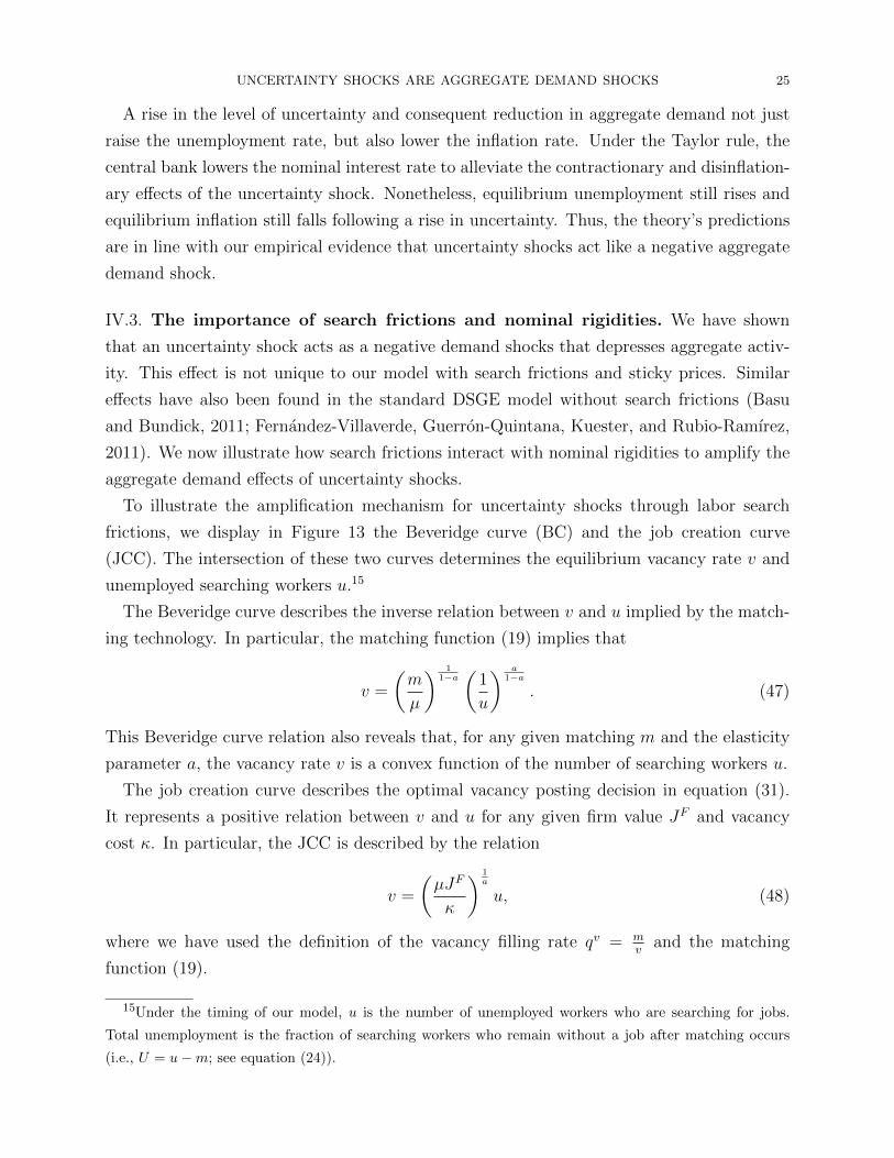
A rise in the level of uncertainty and consequent reduction in aggregate demand not just

raise the unemployment rate, but also lower the inflation rate. Under the Taylor rule, the

central bank lowers the nominal interest rate to alleviate the contractionary and disinflation-

ary effects of the uncertainty shock. Nonetheless, equilibrium unemployment still rises and

equilibrium inflation still falls following a rise in uncertainty. Thus, the theory’s predictions

are in line with our empirical evidence that uncertainty shocks act like a negative aggregate

demand shock.

IV.3. The importance of search frictions and nominal rigidities. We have shown

that an uncertainty shock acts as a negative demand shocks that depresses aggregate activ-

ity. This effect is not unique to our model with search frictions and sticky prices. Similar

effects have also been found in the standard DSGE model without search frictions (Basu

and Bundick, 2011; Fernandez-Villaverde, Guerron-Quintana, Kuester, and Rubio-Ramırez,

2011). We now illustrate how search frictions interact with nominal rigidities to amplify the

aggregate demand effects of uncertainty shocks.

To illustrate the amplification mechanism for uncertainty shocks through labor search

frictions, we display in Figure 13 the Beveridge curve (BC) and the job creation curve

(JCC). The intersection of these two curves determines the equilibrium vacancy rate v and

unemployed searching workers u.15

The Beveridge curve describes the inverse relation between v and u implied by the match-

ing technology. In particular, the matching function (19) implies that

v =

(m

µ

) 11−a(

1

u

) a1−a

. (47)

This Beveridge curve relation also reveals that, for any given matching m and the elasticity

parameter a, the vacancy rate v is a convex function of the number of searching workers u.

The job creation curve describes the optimal vacancy posting decision in equation (31).

It represents a positive relation between v and u for any given firm value JF and vacancy

cost κ. In particular, the JCC is described by the relation

v =

(µJF

κ

) 1a

u, (48)

where we have used the definition of the vacancy filling rate qv = mv

and the matching

function (19).

15Under the timing of our model, u is the number of unemployed workers who are searching for jobs.

Total unemployment is the fraction of searching workers who remain without a job after matching occurs

(i.e., U = u−m; see equation (24)).

UNCERTAINTY SHOCKS ARE AGGREGATE DEMAND SHOCKS 26

First, consider the labor market equilibrium in our benchmark model. Suppose the initial

(steady-state) equilibrium is at point A in Figure 13. As we have discussed in the previous

section, an increase in uncertainty lowers the value of a job match (i.e., JF declines) through

the aggregate demand channel and real wage rigidities amplify the decline in firm value.

Thus, the JCC rotates downward, leading to a new equilibrium at point B, with a lower

vacancy rate and a higher unemployment rate. This downward rotation of the JCC predicted

by the theory is consistent with the empirical responses of the labor market tightness (i.e.,

the v-u ratio) shown in Figure 10.

Now, consider a counterfactual economy with a smaller cost of vacancy posting κ. In such

an economy, search frictions are less important than in our benchmark economy. If vacancy

costs are smaller, firms will post more vacancies, implying a higher job finding rate for a

searching worker.16 From equation (48), a lower value of κ implies a higher value of v for

any given u. Thus, the job creation curve (the solid black line denoted by JCC ′) is steeper

than that in the benchmark economy (the solid blue line denoted by JCC). Accordingly,

the labor-market equilibrium implies a higher vacancy rate and a lower unemployment rate

(point A′). When the level of uncertainty increases, the job creation curve rotates downward

along the Beveridge curve, reaching the new equilibrium at point B′. As in the benchmark

model, the increase in uncertainty lowers the vacancy rate and raises the unemployment rate.

But because the Beveridge curve represents a convex relation between v and u, the increase

in unemployment in this counterfactual economy with a lower vacancy cost is smaller than

that in the benchmark economy.

The quantitative importance of having both search frictions and nominal rigidities is il-

lustrated in Figure 14. The figure shows the impulse responses of unemployment following

a technology uncertainty shock. The solid line indicates the impulse responses of unem-

ployment in the calibrated benchmark DSGE model with both search frictions and nominal

rigidities. The dashed line shows the impulse responses in the flexible-price model (with

Ωp = 0 imposed). The dashed and dotted line shows the impulse responses in a model that

is otherwise identical to the benchmark model except that the vacancy cost parameter κ is

set to a smaller value (0.05 instead of the benchmark calibration of 0.14).

When prices are flexible, a technology uncertainty shock leads to an increase in unem-

ployment, although the magnitude of the increase is about one-sixth as large as that in the

benchmark model with sticky prices (see the dashed line in the figure). This finding

The figure reveals that the response of unemployment to a technology uncertainty shock in

the benchmark model is about 3 times as large as that in a model with a smaller magnitude

16Our model does not completely nest the standard RBC model with a spot labor market. In the extreme

case with κ = 0, the vacancy-posting decision problem is not well defined.

UNCERTAINTY SHOCKS ARE AGGREGATE DEMAND SHOCKS 27

of search frictions and about 6 times as large as that in a model with flexible prices. These

comparisons reveal that, absent either search frictions or nominal rigidities, the effects of

uncertainty shocks on unemployment would be substantially muted.

V. Conclusion

In this paper, we study the macroeconomic effects of uncertainty shocks and show that

uncertainty shocks act like aggregate demand shocks both in the data and in a DSGE model

with search frictions and sticky prices.

Using two clean measures of uncertainty from survey data, we have documented robust

evidence that an increase in the level of uncertainty leads to a rise in unemployment and de-

clines in inflation and the nominal interest rate. This result is robust to alternative measures

of uncertainty, alternative identification strategies, and alternative model specifications.

To help understand the transmission mechanisms of uncertainty shocks, we present a

DSGE model with search frictions and nominal rigidities. We show that interactions between

search frictions and nominal rigidities help significantly amplify the macroeconomic effects of

uncertainty shocks. Absent either frictions, the recessionary effects of an uncertainty shock

would be substantially muted. Consistent with the evidence, our DSGE model predicts that

an uncertainty shock—regardless of its source—raises unemployment and lowers inflation

and the nominal interest rate, and thus acts like a negative aggregate demand shock.

To highlight the aggregate demand effects of uncertainty shocks, we have focused on a

stylized model that abstracts from some realistic and potentially important features of the

actual economy. For example, the model does not have endogenous capital accumulation and

is thus not designed to studying the effects of uncertainty shocks on business investment. To

the extent that investment adjustments are costly, investors are likely to cut back investment

expenditures when they face higher levels of uncertainty. Thus, incorporating endogenous

capital accumulation in our model with search frictions may have important implications for

the quantitative magnitude of the responses of potential and equilibrium output. However,

in light of several recent studies in the literature (Basu and Bundick, 2011; Fernandez-

Villaverde, Guerron-Quintana, Kuester, and Rubio-Ramırez, 2011), incorporating capital

accumulation is unlikely to change the qualitative transmission mechanism of uncertainty

shocks that we have identified in this paper.

In our model, uncertainty shocks raise equilibrium unemployment by lowering the value of

job matches, thus reducing job creation. Meanwhile, we have assumed that the job separa-

tion rate is exogenous. Therefore, the responses of equilibrium vacancy and unemployment

represent a movement along the downward-sloping Beveridge curve. A more realistic model

UNCERTAINTY SHOCKS ARE AGGREGATE DEMAND SHOCKS 28

should incorporate endogenous job separation along the lines of den Haan, Ramey, and Wat-

son (2000) and Walsh (2005), which is likely to further strengthen the aggregate demand

effects of uncertainty shocks that we have studied in this paper. This should prove a fruitful

avenue that we intend to pursue in future research.

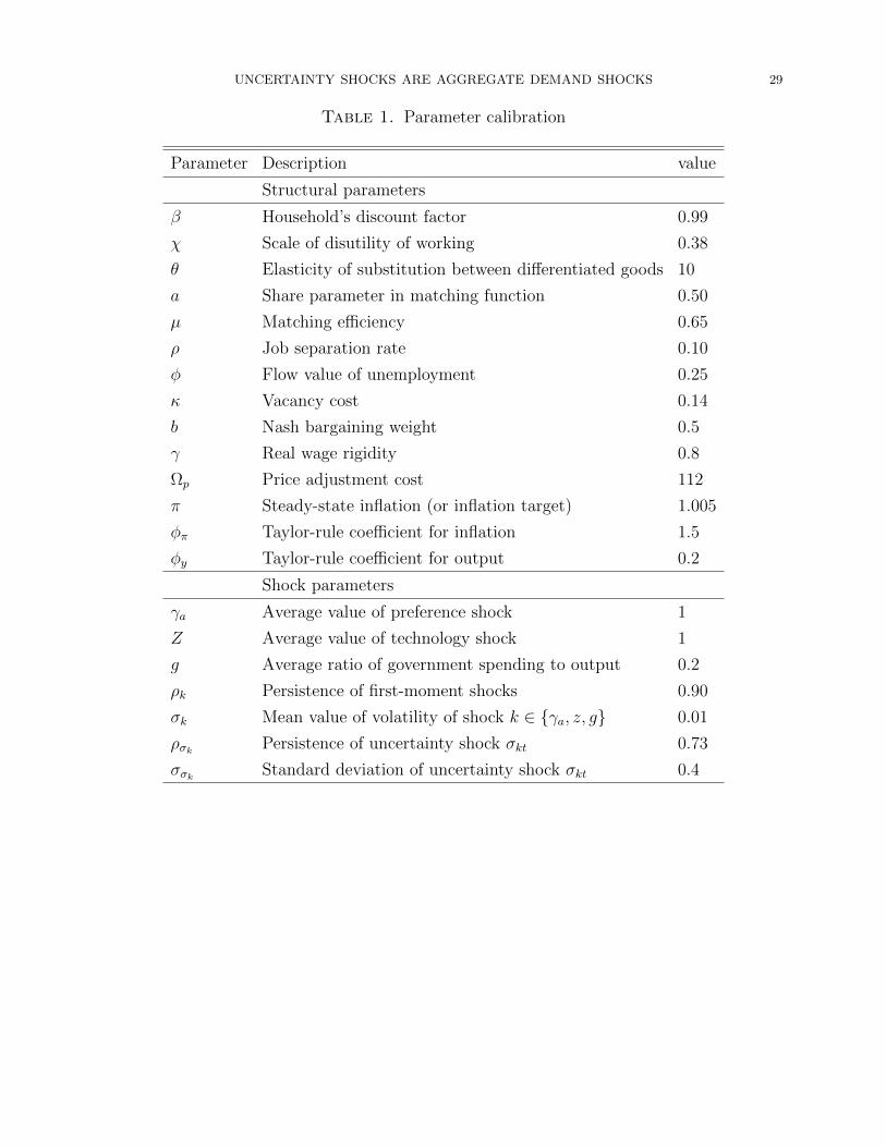
UNCERTAINTY SHOCKS ARE AGGREGATE DEMAND SHOCKS 29

Table 1. Parameter calibration

Parameter Description value

Structural parameters

β Household’s discount factor 0.99

χ Scale of disutility of working 0.38

θ Elasticity of substitution between differentiated goods 10

a Share parameter in matching function 0.50

µ Matching efficiency 0.65

ρ Job separation rate 0.10

φ Flow value of unemployment 0.25

κ Vacancy cost 0.14

b Nash bargaining weight 0.5

γ Real wage rigidity 0.8

Ωp Price adjustment cost 112

π Steady-state inflation (or inflation target) 1.005

φπ Taylor-rule coefficient for inflation 1.5

φy Taylor-rule coefficient for output 0.2

Shock parameters

γa Average value of preference shock 1

Z Average value of technology shock 1

g Average ratio of government spending to output 0.2

ρk Persistence of first-moment shocks 0.90

σk Mean value of volatility of shock k ∈ γa, z, g 0.01

ρσk Persistence of uncertainty shock σkt 0.73

σσk Standard deviation of uncertainty shock σkt 0.4

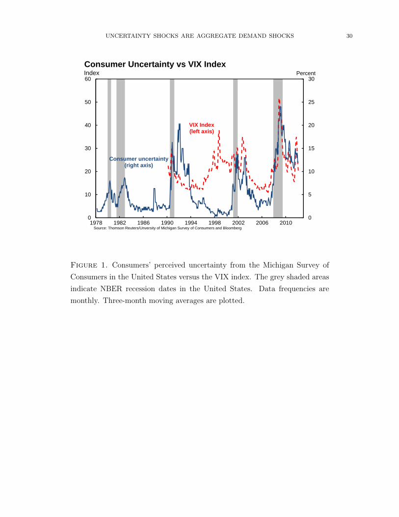
UNCERTAINTY SHOCKS ARE AGGREGATE DEMAND SHOCKS 30

0

5

10

15

20

25

30

0

10

20

30

40

50

60

1978 1982 1986 1990 1994 1998 2002 2006 2010

IndexConsumer Uncertainty vs VIX Index

Percent

Consumer uncertainty(right axis)

VIX Index(left axis)

Source: Thomson Reuters/Unversity of Michigan Survey of Consumers and Bloomberg

Figure 1. Consumers’ perceived uncertainty from the Michigan Survey of

Consumers in the United States versus the VIX index. The grey shaded areas

indicate NBER recession dates in the United States. Data frequencies are

monthly. Three-month moving averages are plotted.

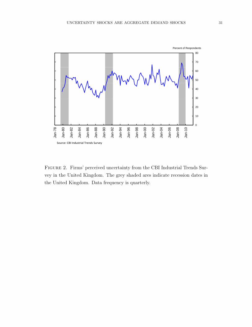
UNCERTAINTY SHOCKS ARE AGGREGATE DEMAND SHOCKS 31

Percent of Respondents

70

80

50

60

30

40

20

30

0

10

78 80 82 84 86 88 90 92 94 96 98 00 02 04 06 08 10

Jan-

7

Jan-

8

Jan-

8

Jan-

8

Jan-

8

Jan-

8

Jan-

9

Jan-

9

Jan-

9

Jan-

9

Jan-

9

Jan-

0

Jan-

0

Jan-

0

Jan-

0

Jan-

0

Jan-

1

Source: CBI Industrial Trends Survey

Figure 2. Firms’ perceived uncertainty from the CBI Industrial Trends Sur-

vey in the United Kingdom. The grey shaded ares indicate recession dates in

the United Kingdom. Data frequency is quarterly.

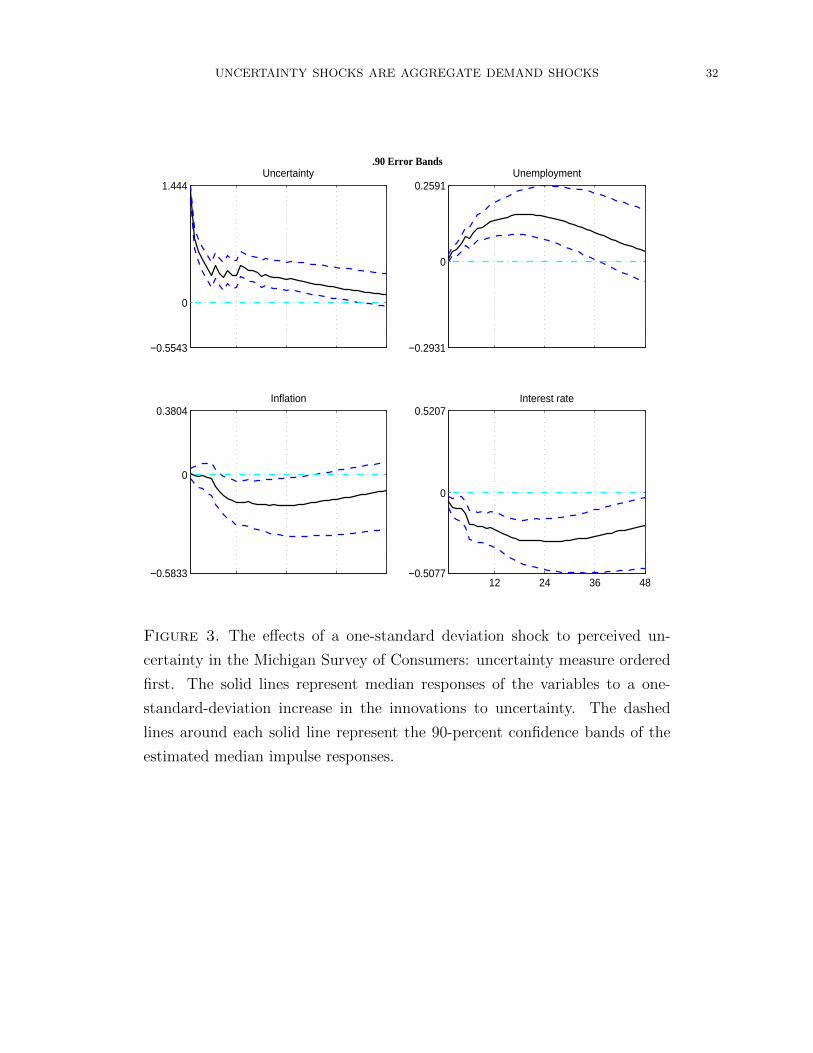
UNCERTAINTY SHOCKS ARE AGGREGATE DEMAND SHOCKS 32

−0.5543

0

1.444Uncertainty

−0.2931

0

0.2591Unemployment

−0.5833

0

0.3804Inflation

12 24 36 48−0.5077

0

0.5207Interest rate

.90 Error Bands

Figure 3. The effects of a one-standard deviation shock to perceived un-

certainty in the Michigan Survey of Consumers: uncertainty measure ordered

first. The solid lines represent median responses of the variables to a one-

standard-deviation increase in the innovations to uncertainty. The dashed

lines around each solid line represent the 90-percent confidence bands of the

estimated median impulse responses.

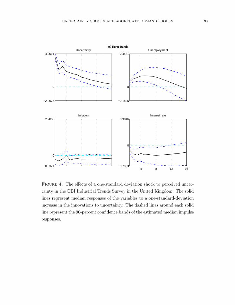
UNCERTAINTY SHOCKS ARE AGGREGATE DEMAND SHOCKS 33

−2.0673

0

4.9014Uncertainty

−0.1896

0

0.4481Unemployment

−0.6371

0

2.2056Inflation

4 8 12 16−0.7053

0

0.9046Interest rate

.90 Error Bands

Figure 4. The effects of a one-standard deviation shock to perceived uncer-

tainty in the CBI Industrial Trends Survey in the United Kingdom. The solid

lines represent median responses of the variables to a one-standard-deviation

increase in the innovations to uncertainty. The dashed lines around each solid

line represent the 90-percent confidence bands of the estimated median impulse

responses.

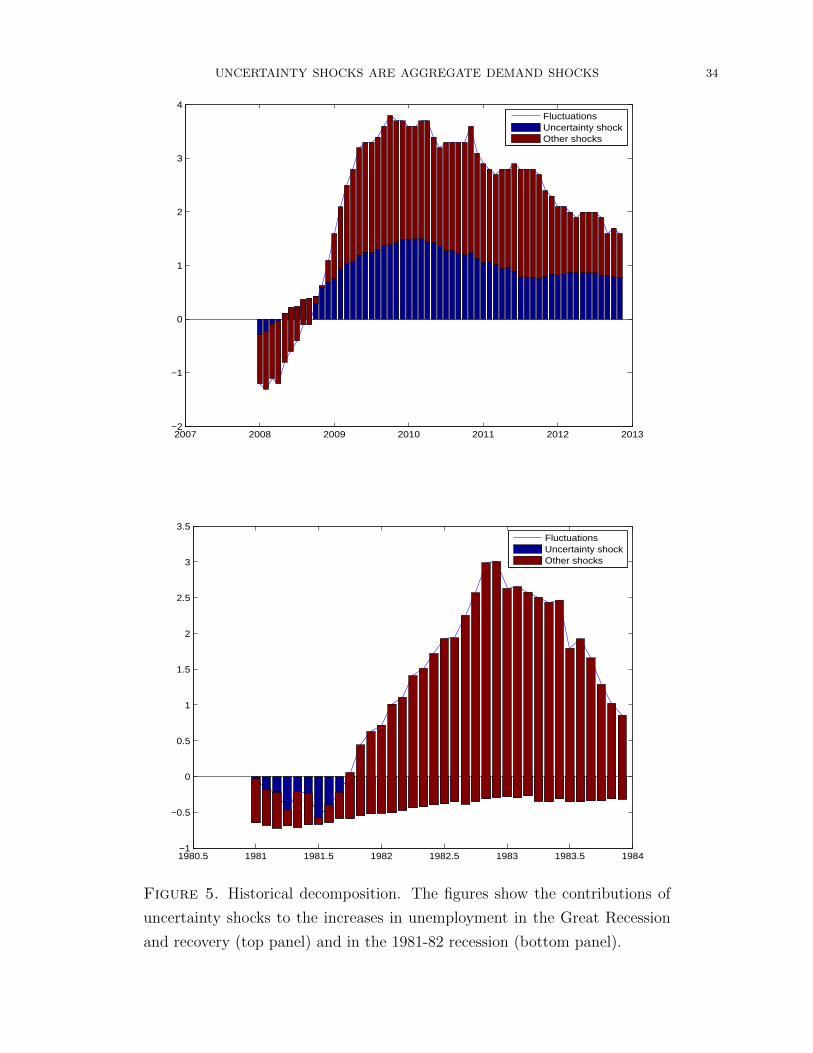
UNCERTAINTY SHOCKS ARE AGGREGATE DEMAND SHOCKS 34

2007 2008 2009 2010 2011 2012 2013−2

−1

0

1

2

3

4

FluctuationsUncertainty shockOther shocks

1980.5 1981 1981.5 1982 1982.5 1983 1983.5 1984−1

−0.5

0

0.5

1

1.5

2

2.5

3

3.5

FluctuationsUncertainty shockOther shocks

Figure 5. Historical decomposition. The figures show the contributions of

uncertainty shocks to the increases in unemployment in the Great Recession

and recovery (top panel) and in the 1981-82 recession (bottom panel).

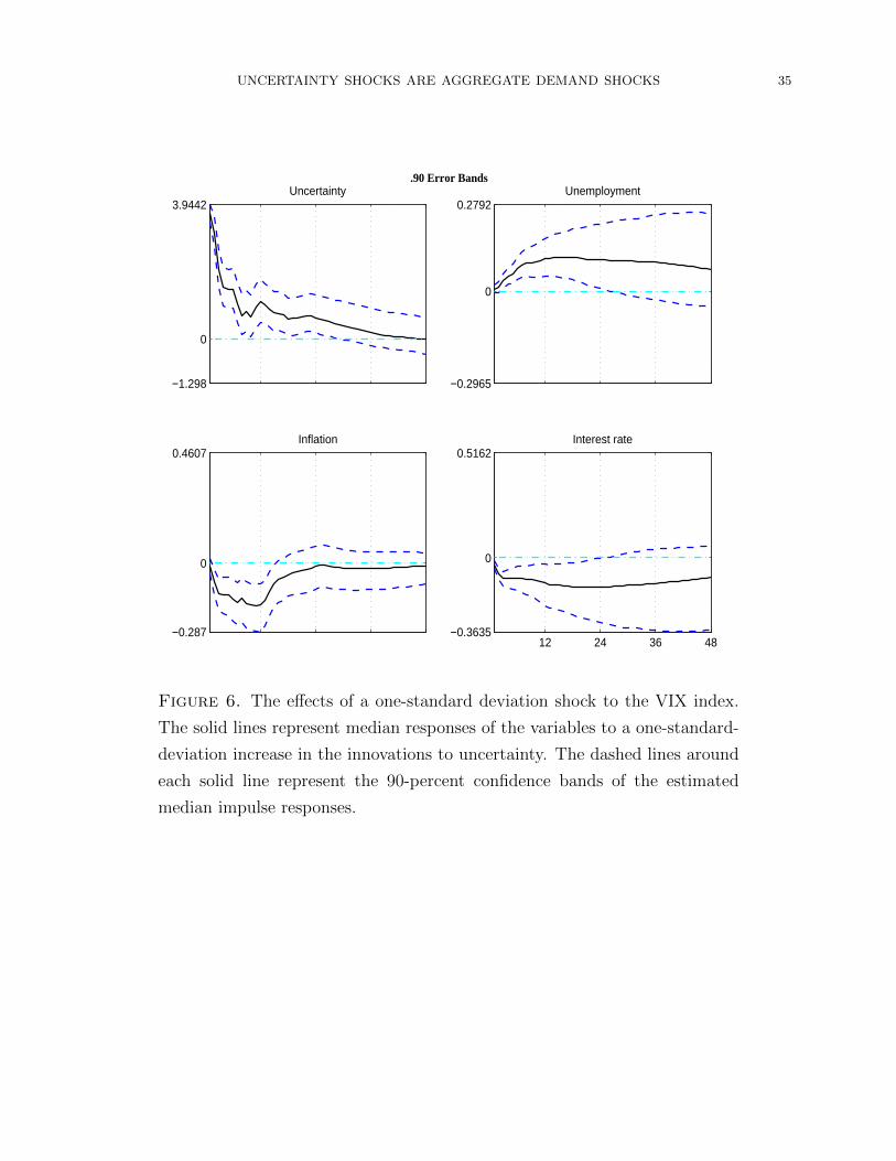
UNCERTAINTY SHOCKS ARE AGGREGATE DEMAND SHOCKS 35

−1.298

0

3.9442Uncertainty

−0.2965

0

0.2792Unemployment

−0.287

0

0.4607Inflation

12 24 36 48−0.3635

0

0.5162Interest rate

.90 Error Bands

Figure 6. The effects of a one-standard deviation shock to the VIX index.

The solid lines represent median responses of the variables to a one-standard-

deviation increase in the innovations to uncertainty. The dashed lines around

each solid line represent the 90-percent confidence bands of the estimated

median impulse responses.

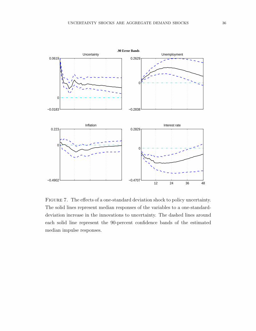
UNCERTAINTY SHOCKS ARE AGGREGATE DEMAND SHOCKS 36

−0.0183

0

0.0619Uncertainty

−0.2838

0

0.2629Unemployment

−0.4902

0

0.223Inflation

12 24 36 48−0.4707

0

0.2829Interest rate

.90 Error Bands

Figure 7. The effects of a one-standard deviation shock to policy uncertainty.

The solid lines represent median responses of the variables to a one-standard-

deviation increase in the innovations to uncertainty. The dashed lines around

each solid line represent the 90-percent confidence bands of the estimated

median impulse responses.

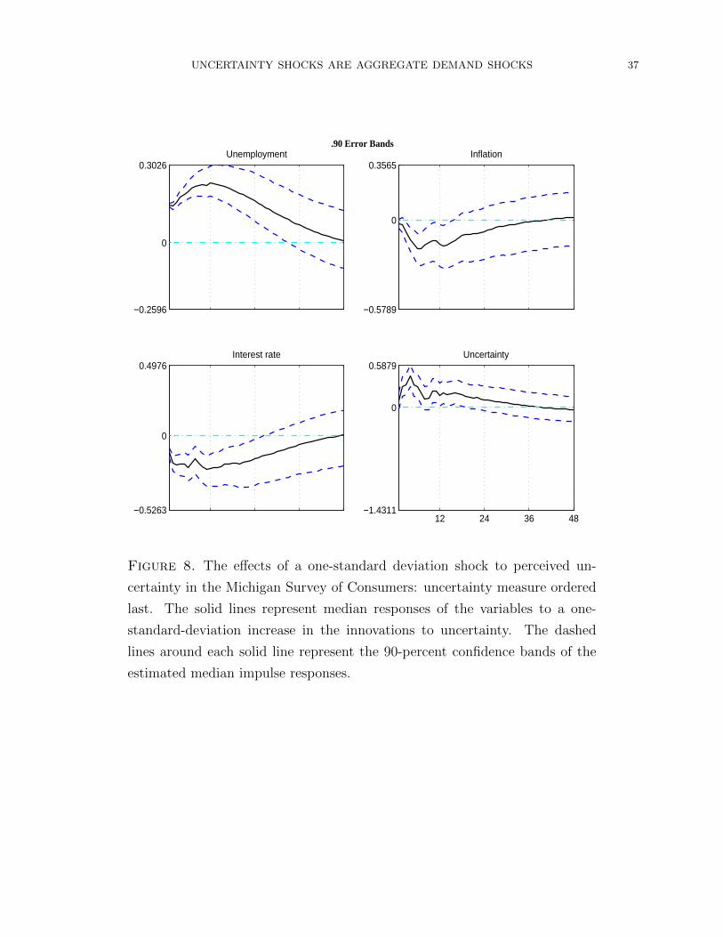
UNCERTAINTY SHOCKS ARE AGGREGATE DEMAND SHOCKS 37

−0.2596

0

0.3026Unemployment

−0.5789

0

0.3565Inflation

−0.5263

0

0.4976Interest rate

12 24 36 48−1.4311

0

0.5879Uncertainty

.90 Error Bands

Figure 8. The effects of a one-standard deviation shock to perceived un-

certainty in the Michigan Survey of Consumers: uncertainty measure ordered

last. The solid lines represent median responses of the variables to a one-

standard-deviation increase in the innovations to uncertainty. The dashed

lines around each solid line represent the 90-percent confidence bands of the

estimated median impulse responses.

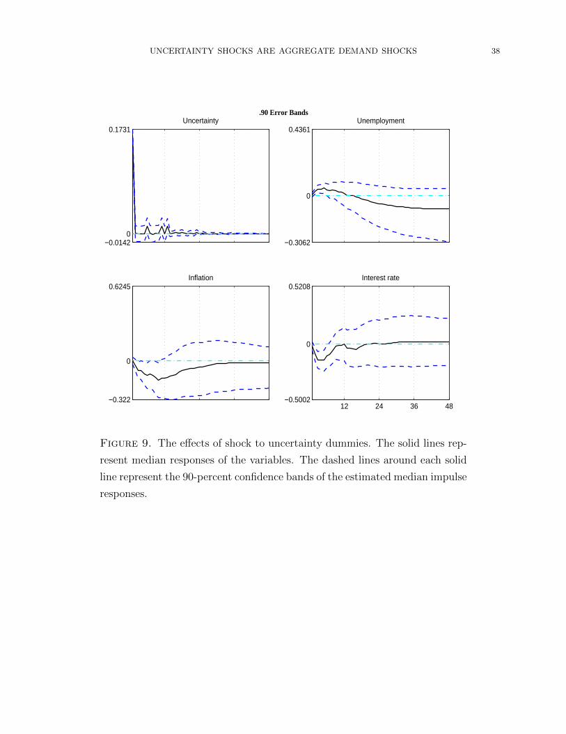
UNCERTAINTY SHOCKS ARE AGGREGATE DEMAND SHOCKS 38

−0.01420

0.1731Uncertainty

−0.3062

0

0.4361Unemployment

−0.322

0

0.6245Inflation

12 24 36 48−0.5002

0

0.5208Interest rate

.90 Error Bands

Figure 9. The effects of shock to uncertainty dummies. The solid lines rep-

resent median responses of the variables. The dashed lines around each solid

line represent the 90-percent confidence bands of the estimated median impulse

responses.

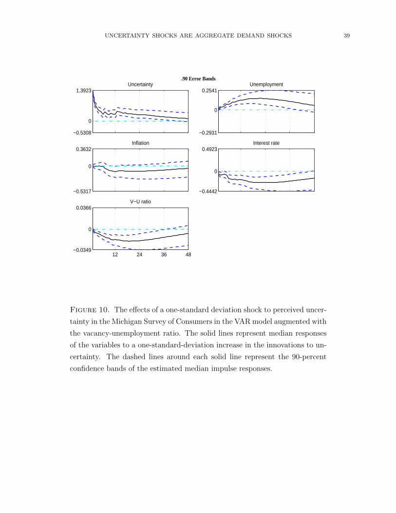
UNCERTAINTY SHOCKS ARE AGGREGATE DEMAND SHOCKS 39

−0.5308

0

1.3923Uncertainty

−0.2931

0

0.2541Unemployment

−0.5317

0

0.3632Inflation

−0.4442

0

0.4923Interest rate

12 24 36 48−0.0349

0

0.0366V−U ratio

.90 Error Bands

Figure 10. The effects of a one-standard deviation shock to perceived uncer-

tainty in the Michigan Survey of Consumers in the VAR model augmented with

the vacancy-unemployment ratio. The solid lines represent median responses

of the variables to a one-standard-deviation increase in the innovations to un-

certainty. The dashed lines around each solid line represent the 90-percent

confidence bands of the estimated median impulse responses.

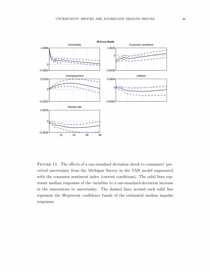
UNCERTAINTY SHOCKS ARE AGGREGATE DEMAND SHOCKS 40

−0.4853

0

1.3986Uncertainty

−3.6435

0

1.8426Consumer sentiment

−0.2623

0

0.2243Unemployment

−0.6062

0

0.3654Inflation

12 24 36 48−0.4835

0

0.4816Interest rate

.90 Error Bands

Figure 11. The effects of a one-standard deviation shock to consumers’ per-

ceived uncertainty from the Michigan Survey in the VAR model augmented

with the consumer sentiment index (current conditions). The solid lines rep-

resent median responses of the variables to a one-standard-deviation increase

in the innovations to uncertainty. The dashed lines around each solid line

represent the 90-percent confidence bands of the estimated median impulse

responses.

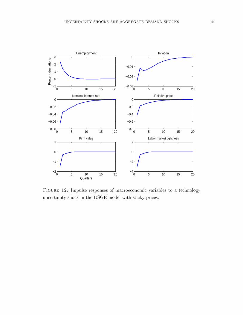
UNCERTAINTY SHOCKS ARE AGGREGATE DEMAND SHOCKS 41

0 5 10 15 20−1

0

1

2

3Unemployment

Pe

rce

nt d

evi

atio

ns

0 5 10 15 20−0.03

−0.02

−0.01

0Inflation

0 5 10 15 20−0.08

−0.06

−0.04

−0.02

0Nominal interest rate

0 5 10 15 20−0.8

−0.6

−0.4

−0.2

0Relative price

0 5 10 15 20−2

−1

0

1Firm value

Quarters0 5 10 15 20

−4

−2

0

2Labor market tightness

Figure 12. Impulse responses of macroeconomic variables to a technology

uncertainty shock in the DSGE model with sticky prices.

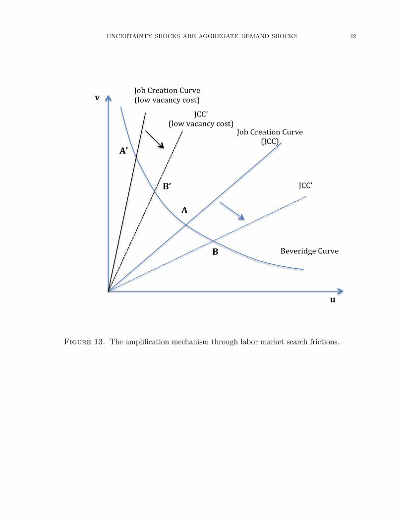
UNCERTAINTY SHOCKS ARE AGGREGATE DEMAND SHOCKS 42

A

A’

B

B’

Beveridge Curve

Job Creation Curve (JCC)

JCC’

Job Creation Curve (low vacancy cost)

JCC’ (low vacancy cost)

u

v

Figure 13. The amplification mechanism through labor market search frictions.

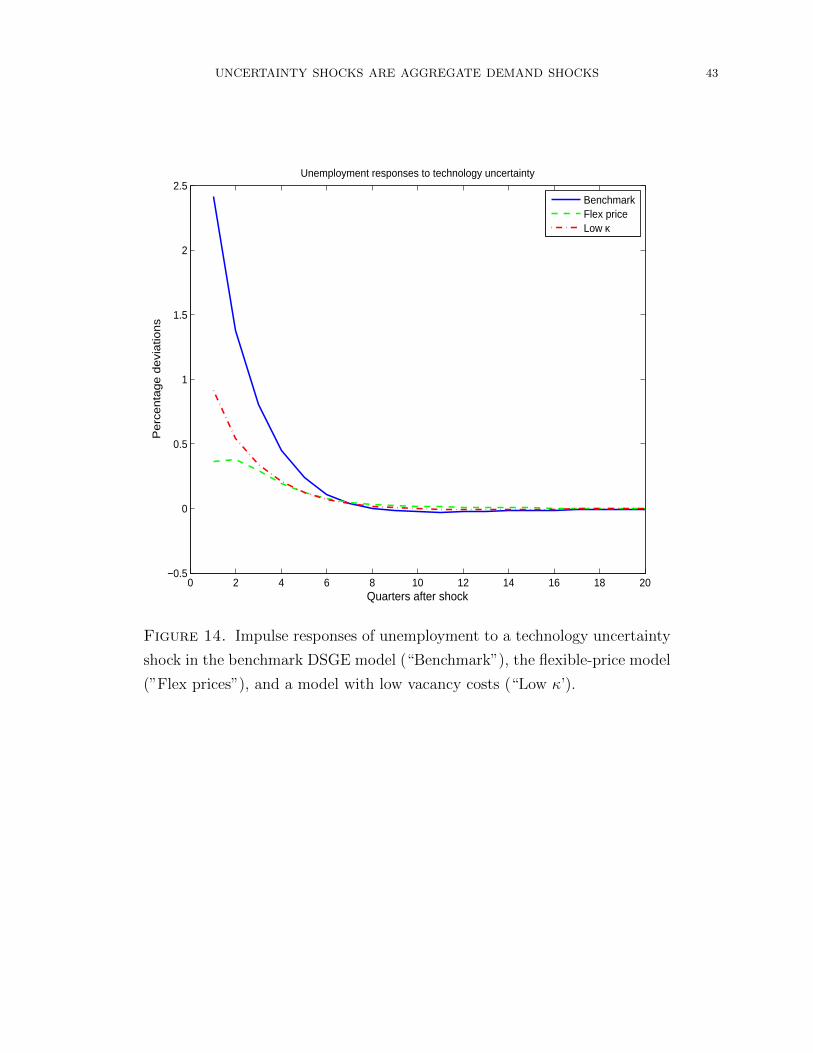
UNCERTAINTY SHOCKS ARE AGGREGATE DEMAND SHOCKS 43

0 2 4 6 8 10 12 14 16 18 20−0.5

0

0.5

1

1.5

2

2.5

Quarters after shock

Pe

rce

nta

ge

de

via

tion

s

Unemployment responses to technology uncertainty

BenchmarkFlex priceLow κ

Figure 14. Impulse responses of unemployment to a technology uncertainty

shock in the benchmark DSGE model (“Benchmark”), the flexible-price model

(”Flex prices”), and a model with low vacancy costs (“Low κ’).

UNCERTAINTY SHOCKS ARE AGGREGATE DEMAND SHOCKS 44

References

Alexopoulos, M., and J. Cohen (2009): “Uncertain Times, Uncertain Measures,” Uni-

versity of Toronto Department of Economics Working Paper 352.

Arellano, C., Y. Bai, and P. Kehoe (2011): “Financial Markets and Fluctuations in

Uncertainty,” Federal Reserve Bank of Minneapolis Research Department Staff Report.

Auerbach, A. J., and Y. Gorodnichenko (2012): “Measuring the Output Responses

to Fiscal Policy,” American Economic Journal: Economic Policy, 4, 1–27.

Bachmann, R., S. Elstner, and E. Sims (2011): “Uncertainty and Economic Activity:

Evidence from Business Survey Data,” University of Michigan Working Paper.

Bachmann, R., and G. Moscarini (2011): “Business Cycles and Endogenous Uncer-

tainty,” Yale University Working Paper.

Baker, S. R., N. Bloom, and S. J. Davis (2011): “Measuring Economic Policy Uncer-

tainty,” Stanford University Working Paper.

Barro, R. J. (2006): “Rare Disasters and Asset Markets in the Twentieth Century,”

Quarterly Journal of Economics, 121(3), 823–866.

Basu, S., and B. Bundick (2011): “Uncertainty Shocks in a Model of Effective Demand,”

Boston College Working Paper.

Basu, S., and J. G. Fernald (1997): “Returns to Scale in U.S. Production: Estimates

and Implications,” Journal of Political Economy, 105(2), 249–283.

Bernanke, B. S. (1983): “Irreversibility, Uncertainty, and Cyclical Investment,” Quarterly

Journal of Economics, 98(1), 85–106.

Bernanke, B. S., M. Gertler, and S. Gilchrist (1999): “The Financial Accelerator

in a Quantitative Business Cycle Framework,” in The Handbook of Macroeconomics, ed.

by J. B. Taylor, and M. Woodford, pp. 1341–1393. Elsevier Science B.V., Amsterdam,

North Holland.

Blanchard, O. J., and J. Galı (2010): “Labor Markets and Monetary Policy: A New

Keynesian Model with Unemployment,” American Economic Journal: Macroeconomics,

2, 1–30.

Bloom, N. (2009): “The Impact of Uncertainty Shocks,” Econometrica, 77(3), 623–685.

Bloom, N., and J. Fernandez-Villaverde (2012): “The Macroeconomics of Uncer-

tainty and Volatility,” Unpublished working paper, Stanford University and University of

Pennsylvania.

Bloom, N., M. Floetotto, N. Jaimovich, I. Saporta-Eksten, and S. J. Terry

(2012): “Really Uncertain Business Cycles,” NBER Working Paper18245.

Boldrin, M., L. J. Christiano, and J. D. Fisher (2001): “Habit Persistence, Asset

Returns, and the Business Cycle,” American Economic Review, 91(1), 149–166.

UNCERTAINTY SHOCKS ARE AGGREGATE DEMAND SHOCKS 45

Christiano, L., M. Eichenbaum, and C. Evans (2005): “Nominal Rigidities and the

Dynamics Effects of a Shock to Monetary Policy,” Journal of Political Economy, 113, 1–45.

Christiano, L., R. Motto, and M. Rostagno (2012): “Risk Shocks,” Unpublished

manuscript, Northwestern University.

den Haan, W. J., G. Ramey, and J. Watson (2000): “Job Destruction and Propagation

of Shocks,” American Economic Review, 90, 482–498.

Diamond, P. A. (1982): “Aggregate Demand Management in Search Equilibrium,” Journal

of Political Economy, 90(5), 881–894.

Fernandez-Villaverde, J., P. Guerron-Quintana, K. Kuester, and J. Rubio-

Ramırez (2011): “Fiscal Volatility Shocks and Economic Activity,” University of Penn-

sylvania Working Paper.

Gabaix, X. (2012): “Variable Rare Disasters: An Exactly Solved Framework for Ten Puz-

zles in Macro-Finance,” Quarterly Journal of Economics, 127(2), 645–700.

Gertler, M., and A. Trigari (2009): “Unemployment Fluctuations with Staggered Nash

Wage Bargaining,” Journal of Political Economy, 117(1), 38–86.

Gilchrist, S., J. W. Sim, and E. Zakrajsek (2010): “Uncertainty, Financial Frictions,

and Investment Dynamics,” Boston University Working Paper.

Gourio, F. (2012): “Disaster Risk and Business Cycles,” American Economic Review,

102(6), 2734–2766.

Guiso, L., and G. Parigi (1999): “Investment and Demand Uncertainty,” Quarterly

Journal of Economics, 114, 185–227.

Hall, R. E. (2005a): “Employment Fluctuations with Equilibrium Wage Stickiness,”

American Economic Review, 95(1), 50–65.

(2005b): “Employment Fluctuations with Equilibrium Wage Stickiness,” American

Economic Review, 95, 50–65.

Hall, R. E., and P. R. Milgrom (2008): “The Limited Influence of Unemployment on

the Wage Bargain,” American Economic Review, 98,(4), 1653–1674.

Ilut, C. L., and M. Schneider (2011): “Ambiguous Business Cycles,” Working paper,

Duke University and Stanford University.

Leahy, J. V., and T. M. Whited (1996): “The Effect of Uncertainty on Investment:

Some Stylized Facts,” Journal of Money, Credit and Banking, 28(1), 64–83.

Leduc, S., and K. Sill (forthcoming): “Expectations and Economic Fluctuations: An

Analysis Using Survey Data,” Review of Economics and Statistics.

Leduc, S., K. Sill, and T. Stark (2007): “Self-Fulfilling Expectations and the Inflation

of the 1970s: Evidence from the Livingston Survey,” Journal of Monetary Economics,

54(2), 433–459.

UNCERTAINTY SHOCKS ARE AGGREGATE DEMAND SHOCKS 46

Liu, Z., J. Miao, and T. Zha (2013): “Housing Prices and Unemployment: A Struc-

tural Analysis,” Unpublished manuscript, Federal Reserve Bank of San Francisco, Boston

University, and Federal Reserve Bank of Atlanta.

Liu, Z., D. F. Waggoner, and T. Zha (2011): “Sources of Macroeconomic Fluctuations:

A Regime Switching DSGE Approach,” Quantitative Economics, 2, 251–301.

Mortensen, D. T., and C. A. Pissarides (1994): “Job Creation and Job Destruction

in the Theory of Unemployment,” Review of Economic Studies, 61(3), 397–415.

Romer, C. D. (1990): “The Great Crash and the Onset of the Great Depression,” Quarterly

Journal of Economics, 105(3), 597–624.

Rotemberg, J. J. (1982): “Sticky Prices in the United States,” Journal of Political Econ-

omy, 90(6), 1187–1211.

Schaal, E. (2012): “Uncertainty, Productivity and Unemployment in the Great Recession,”

Unpublished manuscript, Federal Reserve Bank of Minneapolis.

Sims, C. A., and T. Zha (1998): “Bayesian Methods for Dynamic Multivariate Models,”

International Economic Review, 39(4), 949–968.

Smets, F., and R. Wouters (2007): “Shocks and Frictions in US Business Cycles: A

Bayesian DSGE Approach,” American Economic Review, 97, 586–606.

Walsh, C. E. (2005): “Labor Market Search, Sticky Prices, and Interest Rate Policies,”

Review of Economic Dynamics, 8, 829–849.

Federal Reserve Bank of San Francisco