Identification of NOE models for a continuously variablesemi-active damper

M. Witters, J. SweversK.U.Leuven, Department of Mechanical Engineering,Celestijnenlaan 300 B, B-3001, Heverlee, Belgiume-mail: maarten.witters@mech.kuleuven.be

AbstractThis paper discusses the identification of nonlinear black-box simulation models for a continuously variable,semi-active damper for a passenger car. Two model classes are considered and compared. While bothclasses have an output error model structure, the first class applies a polynomial approximation function andthe second uses a neural network. The identification procedure automatically selects the regression variablesby means of a state of the art model structure selection technique. Experimental validation of the proposedmethod shows that the obtained models are able to accurately simulate the dynamic damper behaviour.

1 Introduction

In order to improve the comfort and handling characteristics of a conventional passive car suspension, theautomotive industry, often in cooperation with research centers and universities, has invested a lot of effortin developing active and semi-active suspension systems [4]. In fully active suspensions, the conventionalpassive spring-damper combination is replaced by an actuator. The major drawbacks of these type of systemsare their high energy consumption and their limited reliability. As an alternative, semi-active suspension sys-tems have been developed. In these systems, the passive damper is replaced by an electronically controlledvariable damper. Two types of semi-active dampers are currently applied in car suspensions: the magneto-rheological damper, that alters the damping ratio by changing the viscosity of a magneto-rheologic fluid, andthe continuously variable, telescopic hydraulic damper in which the damping ratio is adjusted by changingthe orifice of a current controlled valve.The inherent nonlinear dynamics of these semi-active dampers complicate the controller design. Swevers etal. [14] have developed a parameterized, model-free control structure that can be tuned based on the direc-tions of a test-pilot. However, the road tests required for tuning the controller are time consuming and costly.A full vehicle simulation model, including the semi-active damper dynamics, would allow to overcome thisinconvenience.This paper discusses the identification of dynamic simulation models for a continuously variable, semi-activedamper that can be integrated in a full vehicle simulation model. To the authors knowledge, results on mod-elling and identification of this type of semi-active dampers have not yet been published. In the past, a lot ofeffort has been invested in developing models for passive hydraulic dampers and magneto-rheological (MR)dampers, ranging from complicated physical models [3] to nonlinear black-box models [9], [5], [12]. Someof these models are briefly described in section 3, since these results are useful for the development of theelectro-hydraulic semi-active damper model.Black-box models use general mathematical approximating functions to describe the systems input-outputrelations. Hence, the most important advantages of these modelling techniques are the computational effi-ciency, both in model identification as in simulation, and the limited physical insights required to developthese models. However, one of the most difficult issues in developing a black-box model is the selection of

regression variables. Piroddi and Spinelli [11] have developed an identification procedure based on simu-lation error minimization. This procedure is capable of simultaneously optimizing the model structure andestimate the model parameters. The procedure has been applied by Leva et al. [5] to identify a simulationmodel for the dynamic behaviour of a magneto-rheological damper.In this paper, this state of the art technique for the model structure selection will be applied in the identifi-cation procedures for two classes of nonlinear black box models. The first class uses a polynomial outputerror model structure (POE). However, polynomial models suffer from some inconveniences. Firstly, esti-mating the parameters of a POE model is a difficult task. In order to reduce the computational load, theparameter estimation is performed by using the equivalent polynomial NARX model structure instead of thedesired POE structure. This yields suboptimal values for the model parameters. Secondly, since the numberof candidate regressors in a polynomial model grows exponentially with the number of input variables andpast model outputs, which makes the model structure selection a cumbersome and computationally intensivetask. The polynomial models are said to suffer from the curse of dimensionality.The second model class applies a neural network output error model structure (NNOE) [13] to describe thenonlinear damper dynamics. Nørgard et al. [7] have developed an efficient algorithm to estimate the param-eters of NNOE model. To select the regressors for this model type, the state of the art technique based onsimulation error minimization used to identify the polynomial model, has been adopted.It will be shown that the proposed identification procedure for the neural network based output error modelallows to obtain easily an accurate description of the nonlinear damper dynamics based on input-output mea-surements.The paper is organized as follows. Section 2 describes the considered semi-active damper, while section 3briefly reviews some literature about the modelling of passive and magneto-rheological dampers. The nextsection introduces the considered black box model structures, followed by a discussion on the identificationprocedure that includes the model structure selection algorithm and the parameter estimation method. Theexperimental validation of the identified models is presented in section 6, while the last section containssome conclusions and suggestions for improvements.

2 Working principle of the semi-active damper

A classic passive damper consists of a cylinder filled with oil and a rod connected to a piston, which containsa calibrated restriction called the piston valve (see figure 1 left). The change in volume caused by the rodmoving in or out of the cylinder is compensated for by oil flowing in or out of the accumulator (accu) throughthe base valve. The pressure drop over both the base valve and the piston valve results in a damping forceacting on the piston.The construction of the considered telescopic hydraulic semi-active damper hardware (see figure 1 right)corresponds to that of a passive damper in which the piston and base valve are each replaced by a checkvalve. A current-controlled cvsa-valve1 connects the upper and lower damper chambers. The current tothis valve is limited between i− = 0.29A and i+ = 1.6A, which corresponds to the least and most restrictivepositions of the valve (i.e. open and closed), respectively. When the rod moves upwards (positive rattlevelocity, i.e. rebound of the suspension), the piston check valve closes and oil flows through the cvsa-valve.Because the volume of the rod inside the cylinder reduces, oil is forced from the accumulator into the cylinderthrough the base check valve.When the rod moves downwards (negative rattle velocity, i.e. compression of the suspension), the pistoncheck valve opens. Because the volume of the rod inside the cylinder increases, the base check valve closesand oil flows from the cylinder into the accumulator through the cvsa-valve. A low/high current to thecvsa-valve corresponds to a small/large restriction yielding a low/high damping ratio.

1 cvsa: continuously variable semi-active valve

Figure 1: Working principle of a passive and a semi-active damper.

3 Damper modelling

The electro-hydraulic semi-active damper is an evolution of the conventional passive damper, as explainedin section 2. As a consequence, the two devices exhibit a similar dynamic behaviour, including hysteresisand saturation. Results obtained in the modelling of passive dampers can thus be an interesting source ofinformation for the development of a black-box semi-active damper model.Duym et al. developed a complicated continuous time physical model, see [3] and the references therein.However, the identification of the model parameters is cumbersome and simulation is slow. This motivatedthe application of nonlinear black-box modelling techniques to describe the dynamic damper behaviour. Pa-tel and Dunne compared a neural network based NARX model, using damper velocity and temperature asinputs, with the physical model of Duym. They have shown that the identification is much easier in the firstcase, while obtaining the same level of accuracy with both models [9]. Duym also developed a nonlinearblack-box model based on the restoring force method [2]. He reported that models which include the damperacceleration as input yield a higher accuracy than those using the damper displacement.A lot of effort has been invested in the modelling of magneto-rheological dampers. Spencer et al. [15] pro-posed a grey-box approach using the Bouc-Wen model to describe the hysteresis of the device. More recently,nonlinear black-box modelling techniques have been applied to describe the dynamics of MR dampers. Levaand Piroddi developed a polynomial NARX model, while Savaresi used a neural network based NARX modeland demonstrated that the proposed model outperforms the grey-box model developed by Spencer [12].Savaresi included the damper displacement and velocity in the regression vector.In this paper, the aim is to develop a discrete time, black-box simulation model of a electro-hydraulic semi-active damper. Therefore, the performance of two model classes will be compared: polynomial and neuralnetwork based output-error models. Both classes have good approximation characteristics and are able todescribe the complex dynamics of the damper. However, it will be shown that the NNOE is easier to identifyand yields a higher accuracy.

4 Non-linear black box output error models

This section introduces the polynomial and neural network based output error model structures which willbe used to describe the dynamics of the semi-active damper. The identification procedure for both modelclasses is discussed in the next section.

The identification of a discrete time black-box model for a dynamic system [13] is the problem of findinga parameterized relation, g, between the past observed inputs utn = [u(tn−nk), ...,u(tn−nk−nb+1)] and outputs

ytn = [y(tn−1), ...,y(tn−na)] and the current output, y(tn):

y(tn) = g(utn−1 ,ytn−1 ,θ)+ν(tn) (1)

where θ represents the parameter vector and ν an additive noise term. nk refers to a pure delay in thesystem, while na and nb are the number of elements of the output and input variables selected to describethis relation g. Remark that for a multiple input system, u(tn) is a column vector with as many elements asthere are elements as there are input variables. For the considered model structure nb and nk can be selectedindividually for each of the input variables.Sjoberg et al. [13] have shown that the relation g can be split into two mappings: a first one φ maps thepast inputs and outputs into a regression vector ϕ(t) and a second ψ maps the regression vector to the outputspace:

y(tn−1) = ψ(ϕ(tn),θ), (2)

where ϕ(tn) = φ(utn ,ytn).Since the aim is to develop a simulation model for a semi-active damper, no measured outputs are allowed inthe regression vector. Therefore, an output-error (OE) structure is adopted for the regression vector, whichonly depends on the past inputs and model outputs y, up to time tn−1:

ϕ(tn) = φ [ y(tn−1) ... y(tn−na) u(tn−nk) ... u(tn−nk−nb+1) ] (3)

Next, the polynomial and neural network based models and their decomposition in the mapping are dis-cussed.

4.1 Polynomial OE-model

The polynomial output error model is characterized by following equation:

y(tn) =nϕ

∑n=1

(ci

nu,i

∏j=1

upu jj (tn−d j)

ny,i

∏k=1

ypyk(tn−dk)

), (4)

where ci the model parameters and nϕ represents the number of terms. The regression variables of this modelclass are the products of the past observed inputs, u j(tn−d j), and model outputs, y(tn−dk), raised to a certainpower p and subjected to respectively the delays d j and dk. Hence, the ith element of the regression vectoris:

ϕi(tn) =nu,i

∏j=1

upu jj (tn−d j)

ny,i

∏k=1

ypyk(tn−dk) (5)

The second mapping of the model, from the regressor space to the output space, consists of a weighted sumof the regressors. Figure 2 gives a schematic representation of the polynomial model structure. The part infront of the product layer corresponds to the first mapping step of the black-box model. The second mapping,is represented by the summing in the last part of the scheme. The TDL-rectangles represent a tapered delayline applied to the inputs and the model output.

4.2 Neural network based OE-model

A neural network can be defined as a system of neurons that are connected into a network by a set of weights[7]. The principle of a neuron is illustrated in figure 3: it is a processing element that weights its inputs, sumsthem and then returns the corresponding value of its activation function fi. The input 1 represents the bias ofthe weighted sum.The network used in the semi-active damper model is a multi-layer perceptron network. The neurons of sucha network are arranged in layers and the inputs of the neurons in a particular layer are the outputs of the

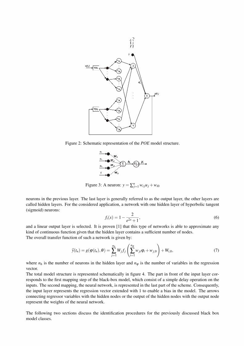
Figure 2: Schematic representation of the POE model structure.

Figure 3: A neuron: y = ∑nj=1 wi ju j +wi0

neurons in the previous layer. The last layer is generally referred to as the output layer, the other layers arecalled hidden layers. For the considered application, a network with one hidden layer of hyperbolic tangent(sigmoid) neurons:

fi(x) = 1− 2e2x +1

, (6)

and a linear output layer is selected. It is proven [1] that this type of networks is able to approximate anykind of continuous function given that the hidden layer contains a sufficient number of nodes.The overall transfer function of such a network is given by:

y(tn) = g(ϕ(tn),θ) =nh

∑j=1

Wj f j

(nϕ

∑i=1

w jiϕi +w j,0

)+Wi,0, (7)

where nh is the number of neurons in the hidden layer and nϕ is the number of variables in the regressionvector.The total model structure is represented schematically in figure 4. The part in front of the input layer cor-responds to the first mapping step of the black-box model, which consist of a simple delay operation on theinputs. The second mapping, the neural network, is represented in the last part of the scheme. Consequently,the input layer represents the regression vector extended with 1 to enable a bias in the model. The arrowsconnecting regressor variables with the hidden nodes or the output of the hidden nodes with the output noderepresent the weights of the neural network.

The following two sections discuss the identification procedures for the previously discussed black boxmodel classes.

Figure 4: Schematic representation of the NNOE model structure.

5 Iterative identification procedure

One of the most difficult aspects of black-box modelling is the selection of the regressor variables: whichvariables and how many elements of each variable are necessary and sufficient to describe the systems dy-namics. A possible source of information is physical insight in the modelled system. From the literaturereview presented in section 3, the damper displacement, velocity, acceleration and of course the control cur-rent are selected as possible inputs.For the identification of the polynomial damper model, a state of the art technique, proposed by Piroddi andSpinelli [11], is applied. The same principe is used to develop an identification procedure for the neuralnetwork based model.

5.1 Identification procedure for the POE model

Several algorithms have been proposed to select the optimal regression vector automatically (see [11] and thereferences therein), but none of them guarantees an optimal solution. In general, these algorithms proceediteratively: at each iteration step a regression variable is added according to some criterion, followed byan estimation of the model parameters. The algorithm continues until a desired accuracy is reached or noimprovement can be realized by adding more regression variables.Here, the regressor selection procedure proposed by Piroddi and Spinelli [11], is used, mainly because ofits successful application to identify a polynomial NARX model for a MR damper [5]. Figure 5 shows aflow diagram of the iterative identification procedure. The different steps of this procedure are now brieflydiscussed.Initialization: At the start of the procedure, the user has to provide the measured input/output data, an initialmodel structure and a set of candidate regression variables. For the polynomial model of equation 4, thecandidate set consists of every possible product of n or less observed inputs and past model outputs, raised toa power pi. The set of candidate regressors is limited by the maximum number of factors, n, the maximumadmitted delay dmax, and power pmax.Before starting the iterative identification procedure, the parameters of the initial model are estimated.Model evaluation: At the beginning of each iteration step, the performance of the model from the previousiteration or of the initial model, when the identification procedure is in its first iteration, is evaluated bycalculating the mean square simulation error (Jk):

Jk =1N

N

∑n=1

(y(tn)− y(tn))2. (8)

Figure 5: Flow diagram of the identification procedure.

Regression vector extension: This part of the procedure selects the additional regression variable that yieldsthe largest model performance improvement. In order to accomplish this, for each possible extension of theregression vector with one element, the model parameters are estimated and the mean square simulation errorperformance index is calculated. The variable that yields the largest reduction of this performance index isselected.Pruning: First, the parameters of all submodels obtained by eliminating one of the regression variables areestimated and evaluated using the above mentioned performance index. Second, if the best reduced modelyields a performance improvement with respect to the model of the previous iteration, it is selected as thenew model. This pruning continues until all models with fewer regressors yield a worse performance thanthe model of the previous iteration step.Stop: The identification procedure is stopped when no model structure can be found that yields a betterperformance, the performance index is below a certain threshold value or a maximum number of iterationsteps is reached.The threshold value used in the stop criterion obviously determines the length of the regression vector: in-creasing this threshold value for the performance index yields a shorter regression vector.

Parameter estimation for the POE modelThe polynomial output error model (equation 4) is nonlinear in the parameters ci, due to including the pastmodel outputs in the regressors. As a consequence, the estimation of the model parameters is a time consum-ing and cumbersome task [11]. Therefore, the parameters estimation will be performed using the equivalentpolynomial NARX model structure, which is linear in the parameters since the past system outputs are usedas regressors instead of the past model outputs:

y(tn) =N

∑n=1

(ci

nu,i

∏j=1

upu jj (tn−d j)

ny,i

∏k=1

ypykk (tn−dk)

). (9)

The parameter estimation problem can be formalized in the following way: given a set of measurement data

ZN = {[u(tn),y(tn)],n = 1, ...,N},

the model parameter vector θ can be found by solving optimization problem:

θ = argminθ{VN(θ ,ZN)}, (10)

where VN(θ ,ZN) is the objective function, expressing the distance between the model output and the mea-sured system output.

For the polynomial NARX model, the corresponding optimization problem can be solved with a linear leastsquares algorithm, see eg. [6], in case a quadratic objective function is used:

VN(θ ,ZN) =1

2N

N

∑n=1

[y(tn)− y(tn|θ)]2. (11)

This method is commonly referred to as the prediction error minimization (PEM). However, a nonlinearmodel estimated using a PEM method, can turn instable when evaluated as an output error model. Therefore,the identification procedure includes a simulation error minimization condition, as explained above.

5.2 Identification procedure for the NNOE model

The identification procedure for the neural network based output error network is analogous to that for thepolynomial model. Obviously, there are however some minor differences, for instance in the selection of theset of candidate regressors and in the parameter estimation.The set of candidate regressors for the neural network model is limited by the number of delays (nk) andelements (na and nb) for each variable that may be included in the regression vector. Hence, the set ofcandidate regressors is much more restricted than in the case of a polynomial model, which results in lessmodels to be compared in the regression vector extension step of the the identification procedure (see figure5). This lowers the computational load and speeds up the identification procedure.In addition, the algorithm does not optimize the network size and number of hidden nodes each time a newregression vector is selected in the extension and pruning steps of the algorithm. The number of hidden nodesis fixed at the beginning. One could include an additional loop in the algorithm to optimize the network size,but this will increase the computational cost considerably. Adequately choosing the size of the network atthe start of the identification procedure, yields satisfactory results.

Parameter estimation for the NNOE modelThe parameters of the neural network are estimated using the methods implemented in the Neural NetworkBased System Identification Toolbox (NNSYSID) [8]. The basic concepts of the applied methods will bereviewed in the following. For a more detailed treatment of the matter, the interested reader is referred to [7].The most commonly used objective function for the estimation of the neural network parameters is followingregularized least squares error criterion [13]:

VN(θ ,ZN) =1

2N

N

∑n=1

[y(tn)− y(tn|θ)]2 +1

2Nθ

T Dθ , (12)

where D is the weight decay term and often chosen as a diagonal matrix D = αI, with α the weight decay.The regularization term in the objective function, 1

2N θ T Dθ , prevents overfitting of network parameters. Theregularization has also a smoothing effect on the objective function and hence will allow the optimizationalgorithm to proceed faster.The least squares problem (12) can be solved numerically by a second order thrust-region optimizationmethod, such as the Levenberg-Marquardt algorithm. Details of this method can be found in general textbooks about numerical optimization, e.g. [6]. The calculation of the derivative of the objective functionwith respect to the network weights can be calculated much more easily for this neural network based modelthan for the polynomial model. Nørgard [7] demonstrated that this derivative can be obtained by filteringthe partial derivative with a time-varying filter. The method can have convergence problems when the filterhas instable roots. However, in proximity of the optimum, this should not occur. This implies that theinitialization of the network weights should be close to the optimum. Therefore, the NNSYSID toolboxinitializes the weights of the NNOE-model with those of the corresponding NNARX-model.

6 Experimental validation

This section discusses the experimental validation of the proposed black-box modelling approaches on apassenger car semi-active damper. First, the measurements and data processing procedures are explained.Next, the parameter estimation and the validation of the obtained models are discussed.

6.1 Experiments and data pre-processing

The measurements are performed on a position controller hydraulic test-rig at the Monroe European Tech-nical Center of Tenneco Automotive: the semi-active damper is excited by a hydraulic actuator, imposinga predefined damper displacement. Figure 6 shows the semi-active damper mounted on the test-rig. Thecomponent of the semi-active damper with the fastest dynamics is the cvsa-valve, which has a response timeof about 10 ms. Therefor, the generated damper force, the realized displacement and the current are sampled10 times faster, at 1000 Hz. The same sampling frequency is used to build the model.

Figure 6: the semi-active damper mounted on the test-rig.

For the displacement a random phase, periodic multisine excitation is used [10]:

xr(t,χ) =F

∑k=−F

|Uk|e j2π fmaxkt/F+ jχk , (13)

with fmax the maximum frequency of the excitation signal, F (∈ N) the number of excited frequency compo-nents and the phases χ = [χ1, ...,χ f ]T of the multisine, a realization of an independent uniformly distributedrandom process on [0,2π). The maximum frequency of the excitation signal is 30 Hz, since the bandwidthof the test-rig actuator is limited. The length of the signal is 65.536 s. The amplitudes are chosen suchthat the damper displacement has a pink spectrum: the excitation amplitudes decreases proportional with thefrequency. Since the response of the semi-active damper is expected to be dependent of the excitation level,measurements at four different excitation levels are performed:

• M 1: displacement between -12.5 mm and 12.5 mm,

• M 2: displacement between -25 mm and 25 mm,

• M 3: displacement between -37.5 mm and 37.5 mm,

• M 4: displacement between -50 mm and 50 mm.

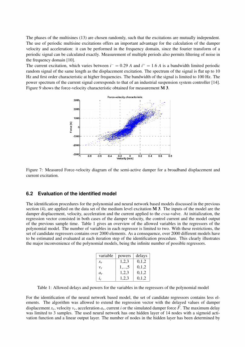
The phases of the multisines (13) are chosen randomly, such that the excitations are mutually independent.The use of periodic multisine excitations offers an important advantage for the calculation of the dampervelocity and acceleration: it can be performed in the frequency domain, since the fourier transform of aperiodic signal can be calculated exactly. Measurement of multiple periods also permits filtering of noise inthe frequency domain [10].The current excitation, which varies between i− = 0.29 A and i+ = 1.6 A is a bandwidth limited periodicrandom signal of the same length as the displacement excitation. The spectrum of the signal is flat up to 10Hz and first order characteristic at higher frequencies. The bandwidth of the signal is limited to 100 Hz. Thepower spectrum of the current signal corresponds to that of an industrial suspension system controller [14].Figure 9 shows the force-velocity characteristic obtained for measurement M 3.

Figure 7: Measured Force-velocity diagram of the semi-active damper for a broadband displacement andcurrent excitation.

6.2 Evaluation of the identified model

The identification procedures for the polynomial and neural network based models discussed in the previoussection (4), are applied on the data set of the medium level excitation M 3. The inputs of the model are thedamper displacement, velocity, acceleration and the current applied to the cvsa-valve. At initialization, theregression vector consisted in both cases of the damper velocity, the control current and the model outputof the previous sample time. Table 1 gives an overview of the allowed variables in the regressors of thepolynomial model. The number of variables in each regressor is limited to two. With these restrictions, theset of candidate regressors contains over 2000 elements. As a consequence, over 2000 different models haveto be estimated and evaluated at each iteration step of the identification procedure. This clearly illustratesthe major inconvenience of the polynomial models, being the infinite number of possible regressors.

variable powers delaysxr 1,2,3 0,1,2vr 1,...,5 0,1,2ar 1,2,3 0,1,2ic 1,2,3 0,1,2

Table 1: Allowed delays and powers for the variables in the regressors of the polynomial model

For the identification of the neural network based model, the set of candidate regressors contains less el-ements. The algorithm was allowed to extend the regression vector with the delayed values of damperdisplacement xr, velocity vr, acceleration ar, current i or the simulated damper force F . The maximum delaywas limited to 3 samples. The used neural network has one hidden layer of 14 nodes with a sigmoid acti-vation function and a linear output layer. The number of nodes in the hidden layer has been determined by

some trial and error and is a compromise between model accuracy and complexity.For the parameter estimation, the first 20000 samples of the data set were used, while the remaining sampleswere used for the model evaluation.To limit the computational time, the identification procedure for the polynomial output error model wasstopped after 50 iteration steps. At that point, the procedure had selected a model containing 30 regressors,which are listed in table 2. The identification procedure for the neural network based model returns following

1 Fd(tn−1) v3r (tn)ic(tn−2) v2

r (tn)ar(tn−2) ar(tn−1)i2c(tn−2)ar(tn)i3c(tn−2) v4

r (tn−2)i2c(tn−2) v2r (tn)Fd(tn−1) xr(tn)ic(tn−2) v3

r (tn)ic(tn−1)ic(tn)Fd(tn−1) vr(tn)i2c(tn−1) xr(tn)vr(tn) ar(tn)F2

d (tn−2) v4r (tn−2)Fd(tn−2)

vr(tn−2)F2d (tn−2) v5

r (tn−2)F2d (tn−2) vr(tn)xr(tn−2) i3c(tn−1)Fd(tn−1) vr(tn−2)ar(tn−2)

ar(tn)F2d (tn−1) v5

r (tn)ic(tn−2) ic(tn)F2d (tn−1) vr(tn)i2c(tn) vr(tn−2)a3

r (tn−1)vr(tn−1)F2

d (tn−2) vr(tn−1)i3c(tn−1) i2c(tn)ar(tn−1) vr(tn)a3r (tn−3) ar(tn)i3c(tn−1)

Table 2: Regressors of the polynomial model

optimal regression vector:

ϕ(tn) = [ F(tn−1) F(tn−2) xr(tn−2) vr(tn−2) vr(tn−3) ar(tn−1) i(tn−2) i(tn−3) ]T .

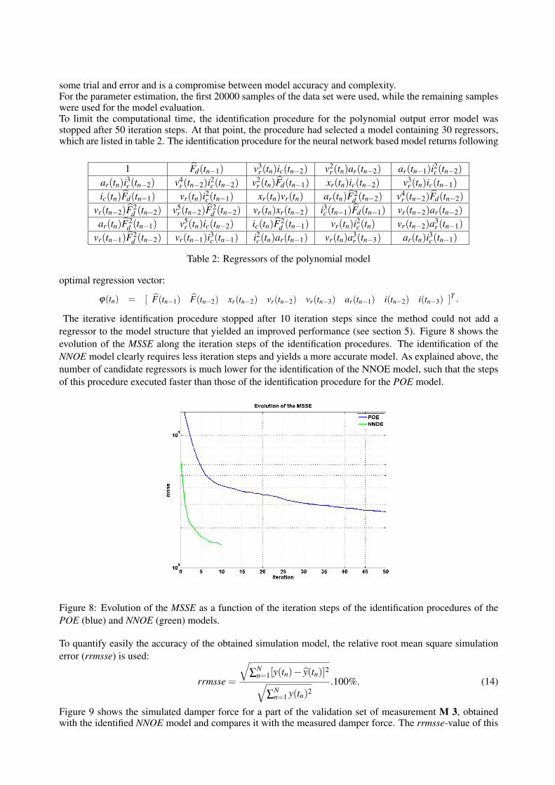
The iterative identification procedure stopped after 10 iteration steps since the method could not add aregressor to the model structure that yielded an improved performance (see section 5). Figure 8 shows theevolution of the MSSE along the iteration steps of the identification procedures. The identification of theNNOE model clearly requires less iteration steps and yields a more accurate model. As explained above, thenumber of candidate regressors is much lower for the identification of the NNOE model, such that the stepsof this procedure executed faster than those of the identification procedure for the POE model.

Figure 8: Evolution of the MSSE as a function of the iteration steps of the identification procedures of thePOE (blue) and NNOE (green) models.

To quantify easily the accuracy of the obtained simulation model, the relative root mean square simulationerror (rrmsse) is used:

rrmsse =

√∑

Nn=1[y(tn)− y(tn)]2√

∑Nn=1 y(tn)2

.100%. (14)

Figure 9 shows the simulated damper force for a part of the validation set of measurement M 3, obtainedwith the identified NNOE model and compares it with the measured damper force. The rrmsse-value of this

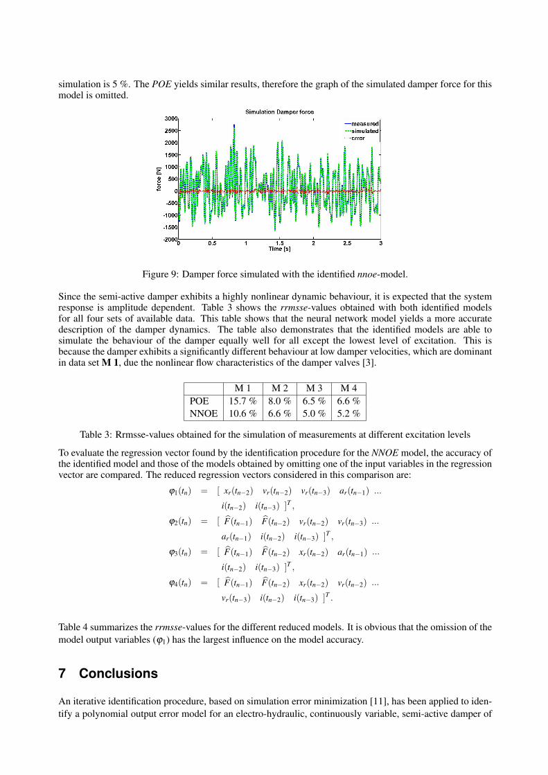
simulation is 5 %. The POE yields similar results, therefore the graph of the simulated damper force for thismodel is omitted.

Figure 9: Damper force simulated with the identified nnoe-model.

Since the semi-active damper exhibits a highly nonlinear dynamic behaviour, it is expected that the systemresponse is amplitude dependent. Table 3 shows the rrmsse-values obtained with both identified modelsfor all four sets of available data. This table shows that the neural network model yields a more accuratedescription of the damper dynamics. The table also demonstrates that the identified models are able tosimulate the behaviour of the damper equally well for all except the lowest level of excitation. This isbecause the damper exhibits a significantly different behaviour at low damper velocities, which are dominantin data set M 1, due the nonlinear flow characteristics of the damper valves [3].

M 1 M 2 M 3 M 4POE 15.7 % 8.0 % 6.5 % 6.6 %NNOE 10.6 % 6.6 % 5.0 % 5.2 %

Table 3: Rrmsse-values obtained for the simulation of measurements at different excitation levels

To evaluate the regression vector found by the identification procedure for the NNOE model, the accuracy ofthe identified model and those of the models obtained by omitting one of the input variables in the regressionvector are compared. The reduced regression vectors considered in this comparison are:

ϕ1(tn) = [ xr(tn−2) vr(tn−2) vr(tn−3) ar(tn−1) ...

i(tn−2) i(tn−3) ]T ,

ϕ2(tn) = [ F(tn−1) F(tn−2) vr(tn−2) vr(tn−3) ...

ar(tn−1) i(tn−2) i(tn−3) ]T ,

ϕ3(tn) = [ F(tn−1) F(tn−2) xr(tn−2) ar(tn−1) ...

i(tn−2) i(tn−3) ]T ,

ϕ4(tn) = [ F(tn−1) F(tn−2) xr(tn−2) vr(tn−2) ...

vr(tn−3) i(tn−2) i(tn−3) ]T .

Table 4 summarizes the rrmsse-values for the different reduced models. It is obvious that the omission of themodel output variables (ϕ1) has the largest influence on the model accuracy.

7 Conclusions

An iterative identification procedure, based on simulation error minimization [11], has been applied to iden-tify a polynomial output error model for an electro-hydraulic, continuously variable, semi-active damper of

ϕ ϕ1 ϕ2 ϕ3 ϕ4

rrmsse 5.0 % 8.8 % 5.5 % 5.9 % 5.3 %

Table 4: Rrmsse-values obtained for the NNOE models with the different regression vectors

a passenger car. However, the selection of candidate regression variables for a polynomial model is a cum-bersome task. The number of possible regression variables for this model class grows exponentially with anincreasing number of input variables and past model outputs.Therefore, an analogous identification procedure was developed to identify neural network based output er-ror model. Due to the good approximation characteristics of sigmoidal neural networks and the efficientparameter estimation algorithms, the efficiency of the identification procedure and the accuracy of the ob-tained model could be improved considerably.The identified NNOE damper model includes damper displacement, velocity, acceleration, current and thesimulated damper force in its regression vector. These variables are available in a multi-body simulation en-vironment, such that the proposed model can be easily incorporated in a full-vehicle simulation model. Thedamper model is able to simulate the measured damper forces accurately, up to a error margin of 5 %, exceptat very low damper velocity. Extension of the working range of the simulation model to lower velocitiesthrough optimal experiment design techniques, will be the subject of future research.To improve the efficiency of the identification procedure even further, there will be investigated whethernonlinear correlation coefficients [16] can be applied as a heuristic to limit the set of candidate regressionvariables at each iteration step.

Acknowledgement

This work is a the result of a collaboration between Tenneco Automotive Europe and the department of themechanical engineering of K.U.Leuven. The financial support of the Institute for the Promotion of Innova-tion by Science and Technology in Flanders (IWT) is gratefully acknowledged.This work also benefits from K.U.Leuven-BOF EF/05/006 Center-of-Excellence Optimization in Engineer-ing and from the Belgian Programme on Interuniversity Attraction Poles, initiated by the Belgian FederalScience Policy Office.

References

[1] G. Cybenco, Approximation by Superpositions of Sigmoidal Functions, Mathematics of Control, Sig-nals, and Systems, vol. 2 (4), 1989, pp. 303-314.

[2] S.W.R Duym, Nonparametric Identification of Nonlinear Mechanical Systems, PhD V.U.B., Dept. ofElectrical Engineering, Brussel, 1998.

[3] S.W.R. Duym, Simulation Tools, Modelling and identification, for an Automotive Shock Absorber in theContext of Vehicle Dynamics, Vehicle System Dynamics, vol. 33 (4), 2000, pp. 261-285.

[4] D. Hrovat, Survey of Advanced Suspension Developments and Related Optimal Control Applications,Automatica, Vol. 33 (10), 1997, pp. 1781-1817.

[5] A. Leva, L.Piroddi, NARX-based technique for the modelling of magneto-rheological damping devices,Smart Materials adn Structures, vol. 11 (1), 2002, pp. 79-88.

[6] J. Nocedal, S.J. Wright, Numerical Optimization, Springer-Verlag, New York, 1999.

[7] M. Nørgaard, O. Ravn, N.K. Poulsen, L.K. Hansen, Neural networks for Modelling and Control ofDynamic Systems, Springer-Verlag, London, UK, 2000.

[8] M. Nørgaard, Neural Network Based System Identification Toolbox, Tech. Report. 00-E-891, Depart-ment of Automation, Technical University of Denmark, 2000.

[9] A. Patel, J.F. Dunne, NARX Neural Network modelling of Hydraulic Suspension Dampers for Steady-state and Variable Temperature Operation, Vehicle System Dynamics, vol 40 (5), 2003, pp. 285-328.

[10] R. Pintelon, J. Schoukens, System Identification: A Frequency Domain Approach, IEEE Press, NewYork, 2001.

[11] L. Piroddi, W. Spinelli, An identification algorithm for polynomial NARX models based on simulationerror minimization, Int. Journal of Control, vol. 76 (17), pp. 1767-1781.

[12] S.M. Savaresi, S. Bittanti, M. Montiglio, Identification of semi-physical and black-box non-linear mod-els: the case of MR-dampers for vehicles control, Automatica, vol. 41, 2005, pp. 113-127.

[13] J. Sjoberg, Q. Zhang, L. Ljung, A. Benveniste, B. Delyon, P-Y. Glorennec, H. Hjalmarsson, A. Juditsky,Nonlinear Black-Box Modeling in System identification: a Unified Overview, Automatica, vol. 31 (12),1995, pp. 1691 - 1724.

[14] J. Swevers, C. Lauwerys, B. Vandersmissen, M. Maes, K. Reybrouck, P. Sas, A model-free controlstructure for the on-line tuning of the semi-active suspension of a passenger car, Mechanical Systemsand Signal Processing, vol. 21, 2007, pp. 1422-1436.

[15] B.F. Spencer Jr., S.J. Dyke, M.K. Sain, J.D. Carlson, Phenomenological Model of a MagnetorheologicalDamper, ASCE Journal of Engineering Mechanics, vol. 123, 1997, pp. 230-238.

[16] Q.M. Zhu, L.F. Zhang, A. Longden, Development of omni-directional correlation functions for nonlin-ear model validation, Automatica, vol. 43 (9), 2007, pp. 1519 - 1531.