Embed Size (px)
Citation preview

Ecole doctorale IAEM Lorraine
Identification of aerodynamiccoefficients from free flight data
Identification de coefficients aerodynamiquesa partir de donnees de vol libre
These presentee et soutenue publiquement le 10 juillet 2015 pour l’obtention du
Doctorat de l’Universite de Lorraine
Mention Automatique, Traitement du Signal et des Images, Genie Informatique
par
Marie Albisser
Composition du jury
President: Edouard LAROCHE Professeur - Universite de Strasbourg
Rapporteurs: Franck CAZAURANG Professeur - Universite de Bordeaux
Guillaume MERCERE Maıtre de Conferences HdR - Universite de Poitiers
Examinateur: Lionel MARRAFFA Directeur de recherche - Agence Spatiale Europeenne
Directeurs: Hugues GARNIER Professeur - Universite de Lorraine
Claude BERNER Directeur de recherche - Institut franco-allemand de recherches deSaint-Louis
Co-directeurs: Magalie THOMASSIN Maıtre de Conferences - Universite de Lorraine
Simona DOBRE Chargee de recherche - Institut franco-allemand de recherches deSaint-Louis
Centre de Recherche en Automatique de NancyUMR 7039 Universite de Lorraine - CNRS
2 rue Jean Lamour, F-54519 Vandoeuvre-les-Nancy, France

Remerciements
Les remerciements ne sont jamais chose facile, au risque de ne pouvoir reellement mettre en evidencel’importance de chacun dans ce qui a donne lieu a ce memoire. Tout d’abord, mes sinceres remer-ciements s’adressent aux membres de mon jury de these, qui m’ont fait l’honneur de participera l’evaluation de ce travail. Guillaume Mercere et Franck Cazaurang pour leur implication entant que rapporteurs, ainsi que Lionel Marraffa et Edouard Laroche pour avoir assure la tached’examinateurs. Merci pour vos remarques constructives et le temps que vous avez consacre a ceprojet.
Je tiens a remercier mes encadrants de l’ISL et du CRAN, Claude Berner, Simona Dobre, MagalieThomassin et Hugues Garnier, pour l’interet qu’ils ont porte a ce travail. Il est essentiel deconstituer une equipe complementaire pour mener a bien tout projet et ces quelques annees decollaboration avec vous m’ont reellement permis de me construire professionnellement. J’adresseun merci tout particulier a Simona et Claude pour leur disponibilite, malgre les imprevus, et leursconseils avises.
Quand on debute une these, on sait toujours ce que l’on cherche mais jamais reellement ce quel’on va trouver. Je peux affirmer avec certitude, des personnes d’exception.
Je souhaite remercier l’ensemble du groupe ABX, pour leur bonne humeur, les delicieuses odeursde tartes au petit matin et leur gentillesse des mes premiers jours au sein de l’equipe.
Merci a la petite bande de l’ISL (les actuels et anciens acolytes), pour les discussions improbablesdu midi, l’humour plus ou moins comprehensible, les perles du net qui nous font toujours esquisserun sourire. . . Dedicace speciale a Vincent, avec qui le covoiturage est propose avec l’option karaoke.
L’annonce d’un sejour en Lorraine n’a pas ete accueillie avec joie. Finalement, ce n’est pas le lieumais les gens qu’on y rencontre qui font la difference. Un grand merci aux “bibis” du CRAN,Christelle, Sam, Vinz, Mag, Hadi, JB, Julien, Simon, . . . pour m’avoir integre dans votre tribudes mon arrivee, les pauses chokys et phi, les soirees nanceennes, votre franc parler, et surtout,pour m’avoir permis de me sentir comme chez moi . . .
Enfin, ces derniers mots de remerciements sont destines a ceux qui, aussi eloignes de mon mondeprofessionnel soient-ils, ont toujours su etre d’un soutien sans faille : la bande d’Hirtzbach, pourtoutes ces soirees animees qui m’ont permis de decompresser; les nunus, pour leur amitie et presencedepuis toutes ces annees; Thibaut, pour cette belle complicite depuis la premiere annee de fac, etqui le dit si bien, a su etre d’un “soutien incommensurable”.

4
Tout ca n’aurait pu etre possible, ni meme envisage, sans mes parents qui ont ete et qui restentdes piliers et des supporters sans limite. Enfin, meme si les choses ni ne se disent ni ne s’ecrivententre nous, le moment est bien choisi pour souligner l’importance de l’oreille attentive qu’elle a suetre, ma twin Mylene, dont l’avis m’a toujours guide dans mes decisions (sauf en sciences).La gratitude ne s’ecrit pas mais se prouve au quotidien, alors a toutes ces personnes, je vous dis atres vite . . .

Contents
Contents I
Notations V
Conferences and publications IX
Introduction 1
1 Aerodynamic testing 91.1 Architectures . . . . . . . . . . . . . . . . . . . . . . . . . . . . . . . . . . . . . . . 10
1.1.1 Space probe . . . . . . . . . . . . . . . . . . . . . . . . . . . . . . . . . . . . 101.1.2 Projectile . . . . . . . . . . . . . . . . . . . . . . . . . . . . . . . . . . . . . 12
1.2 Sabot design . . . . . . . . . . . . . . . . . . . . . . . . . . . . . . . . . . . . . . . 131.2.1 Space probe . . . . . . . . . . . . . . . . . . . . . . . . . . . . . . . . . . . . 131.2.2 Projectile . . . . . . . . . . . . . . . . . . . . . . . . . . . . . . . . . . . . . 13
1.3 Model instrumentation and data acquisition . . . . . . . . . . . . . . . . . . . . . . 141.3.1 Space probe . . . . . . . . . . . . . . . . . . . . . . . . . . . . . . . . . . . . 151.3.2 Projectile . . . . . . . . . . . . . . . . . . . . . . . . . . . . . . . . . . . . . 15
1.4 Open range test facility and measurement techniques . . . . . . . . . . . . . . . . . 161.5 Test conditions . . . . . . . . . . . . . . . . . . . . . . . . . . . . . . . . . . . . . . 18
1.5.1 Space probe . . . . . . . . . . . . . . . . . . . . . . . . . . . . . . . . . . . . 181.5.2 Projectile . . . . . . . . . . . . . . . . . . . . . . . . . . . . . . . . . . . . . 19
1.6 Concluding remarks . . . . . . . . . . . . . . . . . . . . . . . . . . . . . . . . . . . 19
2 Modelling of a vehicle in free flight 212.1 Coordinate systems . . . . . . . . . . . . . . . . . . . . . . . . . . . . . . . . . . . . 212.2 General structure of the model . . . . . . . . . . . . . . . . . . . . . . . . . . . . . 222.3 State equations . . . . . . . . . . . . . . . . . . . . . . . . . . . . . . . . . . . . . . 23
2.3.1 Force and moment equations . . . . . . . . . . . . . . . . . . . . . . . . . . 232.3.2 Kinematic equations . . . . . . . . . . . . . . . . . . . . . . . . . . . . . . . 27
2.4 Aerodynamic coefficients . . . . . . . . . . . . . . . . . . . . . . . . . . . . . . . . . 282.4.1 Force coefficients . . . . . . . . . . . . . . . . . . . . . . . . . . . . . . . . . 282.4.2 Moment coefficients . . . . . . . . . . . . . . . . . . . . . . . . . . . . . . . 292.4.3 Aerodynamic coefficient assumptions . . . . . . . . . . . . . . . . . . . . . . 302.4.4 Descriptions of aerodynamic coefficients . . . . . . . . . . . . . . . . . . . . 31
2.4.4.1 Space probe . . . . . . . . . . . . . . . . . . . . . . . . . . . . . . 312.4.4.2 Projectile . . . . . . . . . . . . . . . . . . . . . . . . . . . . . . . . 33
I
II Contents
2.5 Output equations . . . . . . . . . . . . . . . . . . . . . . . . . . . . . . . . . . . . . 332.6 Concluding remarks . . . . . . . . . . . . . . . . . . . . . . . . . . . . . . . . . . . 34
3 Aerodynamic parameter identification 393.1 Inverse problem . . . . . . . . . . . . . . . . . . . . . . . . . . . . . . . . . . . . . . 393.2 Identification procedure . . . . . . . . . . . . . . . . . . . . . . . . . . . . . . . . . 403.3 Prior knowledge and model implementation . . . . . . . . . . . . . . . . . . . . . . 413.4 Identifiability analysis . . . . . . . . . . . . . . . . . . . . . . . . . . . . . . . . . . 43
3.4.1 A priori identifiability analysis . . . . . . . . . . . . . . . . . . . . . . . . . 443.4.2 A posteriori identifiability analysis . . . . . . . . . . . . . . . . . . . . . . . 453.4.3 Identifiability analysis - application to space probe models . . . . . . . . . . 48
3.4.3.1 A priori identifiability results . . . . . . . . . . . . . . . . . . . . . 483.4.3.2 A posteriori identifiability results . . . . . . . . . . . . . . . . . . 49
3.5 Estimation of aerodynamic parameters . . . . . . . . . . . . . . . . . . . . . . . . . 523.6 Concluding remarks . . . . . . . . . . . . . . . . . . . . . . . . . . . . . . . . . . . 53
4 Application results and discussions 554.1 Space probe . . . . . . . . . . . . . . . . . . . . . . . . . . . . . . . . . . . . . . . . 55
4.1.1 Model’s ability to reproduce the measured output signals . . . . . . . . . . 574.1.2 Evolution of the state variables . . . . . . . . . . . . . . . . . . . . . . . . . 60
4.1.2.1 Total angle of attack and Mach number . . . . . . . . . . . . . . . 604.1.2.2 Polar motion . . . . . . . . . . . . . . . . . . . . . . . . . . . . . . 61
4.1.3 Parametric estimation of the aerodynamic coefficients . . . . . . . . . . . . 624.1.3.1 Drag coefficient . . . . . . . . . . . . . . . . . . . . . . . . . . . . 624.1.3.2 Pitch damping coefficient . . . . . . . . . . . . . . . . . . . . . . . 63
4.2 Projectile . . . . . . . . . . . . . . . . . . . . . . . . . . . . . . . . . . . . . . . . . 654.2.1 Model’s ability to reproduce the measured output signals . . . . . . . . . . 664.2.2 Evolution of the state variables . . . . . . . . . . . . . . . . . . . . . . . . . 69
4.2.2.1 Total angle of attack and Mach number . . . . . . . . . . . . . . . 694.2.2.2 Polar motion . . . . . . . . . . . . . . . . . . . . . . . . . . . . . . 714.2.2.3 Comparison with complementary methods . . . . . . . . . . . . . 72
4.2.3 Parametric estimation of the aerodynamic coefficients . . . . . . . . . . . . 744.2.3.1 Drag coefficient . . . . . . . . . . . . . . . . . . . . . . . . . . . . 754.2.3.2 Roll moment coefficient . . . . . . . . . . . . . . . . . . . . . . . . 764.2.3.3 Pitch moment coefficient slope . . . . . . . . . . . . . . . . . . . . 774.2.3.4 Normal force coefficient . . . . . . . . . . . . . . . . . . . . . . . . 784.2.3.5 Pitch damping coefficient . . . . . . . . . . . . . . . . . . . . . . . 79
4.3 Discussions . . . . . . . . . . . . . . . . . . . . . . . . . . . . . . . . . . . . . . . . 80
Conclusions and perspectives 81
Appendix 85
A Modelling - complementary information 85A.1 Transformation matrices . . . . . . . . . . . . . . . . . . . . . . . . . . . . . . . . . 85
A.1.1 Gravity vector in body axes . . . . . . . . . . . . . . . . . . . . . . . . . . . 87A.2 Rotational kinematic equations . . . . . . . . . . . . . . . . . . . . . . . . . . . . . 87
Contents III
A.3 Attitude representations . . . . . . . . . . . . . . . . . . . . . . . . . . . . . . . . . 88
B Static and dynamic stability 89
C Sedoglavic algorithm 93C.1 Algorithm description . . . . . . . . . . . . . . . . . . . . . . . . . . . . . . . . . . 93C.2 Example . . . . . . . . . . . . . . . . . . . . . . . . . . . . . . . . . . . . . . . . . . 94
List of Figures 95
List of Tables 99
References 101

Notations
ABBREVIATIONS & ACRONYMS
DOF Degrees Of FreedomCFD Computational Fluid DynamicsARFDAS Aeroballistic Research Facility Data Analysis SystemCADRA Comprehensive Automated Data Reduction and Analysis
c.g. center of gravityw.r.t. with respect to
MATHEMATICS, MODELLING & IDENTIFICATION
a variablea vectorA matrixTAA transformation matrix from frame A to frame A
M model structuret time variablex state vectorx0 initial value of the state vectory output vectoru input signal vectorpa aerodynamic coefficient parameter vector/ model parameter vectorp = [x0,pa] parameter vectorp∗ true value of parameter vectorp1 a priori identifiable parameter vectorp2 a posteriori identifiable parameter vector
N number of measurement timesnx number of state variablesny number of outputsnp number of parametersns number of selected free flight test cases
R set of real numbersP set of a priori admissible parametersT set of measurement times
VI Notations
REFERENCE FRAMES
.E Earth axes OxE ,yE ,zE
.B body axes Ox,y,z
.W wind axes OxW ,yW ,zW
PHYSICAL QUANTITIES & VARIABLES
F applied forces vectorF. applied force (N)M applied moment vector about the c.g.M. applied moment about the c.g. (N.m)g gravity (9.8066 m/s2)ρ air density (kg/m3)q dynamic pressure (N/m3)a speed of sound (m/s)m vehicle mass (kg)d vehicle diameter/ projectile caliber (m)L vehicle length (m)S surface reference area (m2)δ fin cant angle (deg)Xcg c.g. position on the x body axis w.r.t. the vehicle nose (m)I inertia matrixIx longitudinal moment of inertia (kg.m2)Iy, Iz transversal moment of inertia (kg.m2)V translational velocity vectorV translational velocity (m/s)vx translational velocity about x body axis (m/s)vy translational velocity about y body axis (m/s)vz translational velocity about z body axis (m/s)M Mach numberα angle of attack (deg)β angle of sideslip (deg)αt total angle of attack (deg)ω angular velocity vectorωx roll rate/ spin rate (deg/s)ωy pitch rate (deg/s)ωz yaw rate (deg/s)φ roll angle (deg)θ pitch angle (deg)ψ yaw angle (deg)xE x component of the c.g. position w.r.t. the Earth frame (m)yE y component of the c.g. position w.r.t. the Earth frame (m)zE z component of the c.g. position w.r.t. the Earth frame (m)
M0 initial launch Mach numberα0 initial angle of attack (deg)
Notations VII
AERODYNAMIC COEFFICIENTS C(x(t),pa) (no dimension)
CX axial force coefficient (body frame)CY sideforce coefficient (body frame)CN = −CZ normal force coefficient (body frame)CD drag coefficient (wind frame)CY w sideforce coefficient (wind frame)CL lift coefficient (wind frame)CLα lift coefficient slopeCypα Magnus force coefficient slopeCl, Cm, Cn roll, pitch, yaw moment coefficientsClp roll damping coefficientClδ roll moment coefficient due to fin cantCmα pitch moment coefficient slope or overturning coefficientCnβ yaw moment coefficient slopeCmq pitch damping coefficientCnr yaw damping coefficientCnpα Magnus moment coefficient slope

Conferences and publications
The main studies perform during the thesis and detailed in this report were submitted and pre-sented at several international congresses and had led to the following publications:
Article in international peer-reviewed journal
Albisser, M., Dobre, S., Berner, C., Thomassin, M. and Garnier, H., Identification of aerody-namic coefficients of a re-entry space vehicle from multiple free flight tests. AIAA Journal ofSpacecraft and Rockets, 2015, to be submitted.
Papers in international peer-reviewed conferences with proceedings
Albisser, M., Dobre, S., Berner, C., Thomassin, M. and Garnier, H., ”Identifiability investiga-tion of the aerodynamic coefficients from free flight tests”, AIAA Atmospheric Flight MechanicsConference, Boston, Massachusetts, 2013.
Albisser, M., Dobre, S., Berner, C., Thomassin, M. and Garnier, H., ”Grey-box identificationof the aerodynamic coefficients from free flight tests”, 13th ECC European Control Conference,Strasbourg, France, 2014.
Albisser, M., Berner, C., Dobre, S., Thomassin, M. and Garnier, H., ”Aerodynamic coefficientsidentification procedure of a finned projectile using magnetometers and videos free flight data”,28th ISB International Symposium on Ballistics, Atlanta, Georgia, 2014.
Dobre, S., Berner, C., Albisser, M. and Saada, F., ”MarcoPolo-R ERC Dynamic Stability Char-acterization. Open Range Free Flight Tests”, 8th European Symposium on Aerothermodynamicsfor Space Vehicles, Lisbon, Portugal, 2015.
Oral presentations in international conferences (without proceedings)
Albisser, M., Dobre, S., Berner, C., Thomassin, M. and Garnier, H., ”Identifiability investigationof the aerodynamic coefficients from free flight tests”, ERNSI, Workshop of the European ResearchNetwork on System Identification, Nancy, France, 2013.
Albisser, M., Berner, C. and Dobre, S., ”Aerodynamic Coefficient Identification Procedure of aReference Finned Projectile”, ISL Scientific Symposium, Saint-Louis, France, 2015.
Oral presentation in a national workshop (without proceedings)
Albisser, M., Dobre, S., Berner, C., Thomassin, M. and Garnier, H., ”Aerodynamic parameteridentification of vehicles in free flight”, Identification Workshop, Paris, France, 2014.

Introduction
Tout mettre en œuvre pour atteindre un objectif, dans tous les sens du terme. Parvenir a unbut precis, un projectile qui touche une cible, une sonde spatiale mise en orbite ou qui atterritsur une surface desiree, par exemple une planete, pour etudier un nouvel environnement en est ledenouement souhaite. Cette finalite est dependante de l’objet lance et ainsi, la connaissance ducomportement en vol de ce dernier reste indispensable a cette reussite. Ce projet aspire, a traversl’identification des coefficients aerodynamiques, a determiner les caracteristiques aerodynamiquesd’un vehicule en vol qu’il soit, un corps de rentree dans l’atmosphere, un drone ou une munition.L’estimation de ces parametres est basee sur des donnees mesurees en vol libre au moyen dedifferentes techniques de mesure. Ce sujet de recherche a ete propose par l’Institut franco allemandde recherches de Saint-Louis (ISL), plus particulierement, par le groupe d’Aerodynamique et deBalistique eXterieure (ABX), s’associant le concours d’un laboratoire universitaire specialise dansle domaine de l’identification qu’est le Centre de Recherche en Automatique de Nancy (CRAN).Ainsi, la collaboration avec l’equipe-projet iModel du departement CID (Controle, Identificationet Diagnostic) traitant l’identification et la modelisation de systemes dynamiques, a cree unecomplementarite des competences avec les aptitudes de l’ISL.
La balistique est la science qui a pour objet d’etudier l’ensemble des phenomenes auxquels estsoumis un projectile, du depart du coup jusqu’a la fin de son interaction avec une cible. Elle peutetre divisee en 4 categories : interieure, intermediaire, exterieure et terminale [Dorrzapft (2010)] :
− la balistique interieure est dediee aux etudes des phenomenes se produisant a l’interieur ducanon, dans le but par exemple, d’ameliorer l’efficacite des systemes de lancement ;
− la balistique intermediaire concerne l’etude des phenomenes lies entre autres aux interactionsexternes sur l’objet en sortie du canon telles que les gaz de combustion, le saut aerodynamiqueou les interferences produites par les sabots maintenant l’objet dans le lanceur. Ce domaineest souvent fusionne avec celui de la balistique exterieure ;
− la balistique exterieure est la phase comprise entre le moment ou l’objet en vol n’est plusperturbe par les turbulences de la bouche du canon et/ou par les interactions externes commela separation des sabots jusqu’a l’impact ;
− en dernier lieu, la balistique terminale traite des etudes liees a l’interaction de l’objet avec lacible.
La presente etude s’inscrit dans le cadre de la balistique exterieure. En fonction des forces agissantsur le vehicule, deux branches de la balistique exterieure se distinguent. D’une part, la balis-
2 Introduction
tique du vide qui ne considere que la force gravitationnelle comme force agissant sur le vehicule.D’autre part, la balistique dans le milieu atmospherique qui etudie l’attitude en vol caracteriseepar l’ensemble des forces et moments qui s’appliquent sur le vehicule. Ces derniers sont directe-ment relies aux coefficients aerodynamiques. Ils representent une contribution essentielle a lamodelisation de nombreux phenomenes et englobent principalement les aspects de resistance, deportance, mais egalement de stabilite. Deux types de stabilite peuvent etre definis et suscitent ungrand nombre d’etudes, particulierement en aerodynamique, ou on distingue la stabilite statiqueet la stabilite dynamique. La stabilite statique decrit la capacite d’un objet a retrouver sa positiond’equilibre apres en avoir ete ecartee alors que la stabilite dynamique considere la tendance dumouvement pour retrouver une position d’equilibre.
En balistique exterieure, l’utilisation des coefficients aerodynamiques pour caracteriser le com-portement d’un objet en vol demeure un sujet de recherche parmi les plus complexes et les plusetudies. Durant ces dernieres decennies, les avancees techniques ont mene au developpement demethodes experimentales et theoriques permettant de quantifier les proprietes aerodynamiques.Plusieurs outils existent et peuvent etre utilises, a savoir :
− les codes numeriques ;
− les essais en soufflerie ;
− les essais en champ de tir.
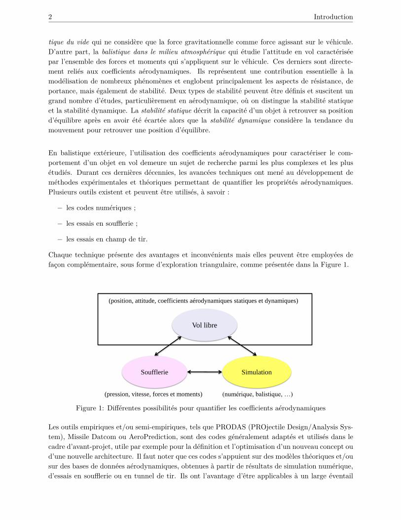
Chaque technique presente des avantages et inconvenients mais elles peuvent etre employees defacon complementaire, sous forme d’exploration triangulaire, comme presentee dans la Figure 1.
Vol libre
Soufflerie Simulation
(pression, vitesse, forces et moments) (numérique, balistique, …)
(position, attitude, coefficients aérodynamiques statiques et dynamiques)
Figure 1: Differentes possibilites pour quantifier les coefficients aerodynamiques
Les outils empiriques et/ou semi-empiriques, tels que PRODAS (PROjectile Design/Analysis Sys-tem), Missile Datcom ou AeroPrediction, sont des codes generalement adaptes et utilises dans lecadre d’avant-projet, utile par exemple pour la definition et l’optimisation d’un nouveau concept oud’une nouvelle architecture. Il faut noter que ces codes s’appuient sur des modeles theoriques et/ousur des bases de donnees aerodynamiques, obtenues a partir de resultats de simulation numerique,d’essais en soufflerie ou en tunnel de tir. Ils ont l’avantage d’etre applicables a un large eventail
Introduction 3
de configurations et permettent d’obtenir rapidement des resultats. Cependant, la determinationdes proprietes aerodynamiques a partir de ces codes est dependante de la qualite de la base dedonnees repertoriee. Afin d’obtenir des estimations suffisamment precises, la configuration etudieedoit etre proche de celle qui a permis de peupler la base de donnees.La simulation numerique, au moyen de codes de calcul CFD (Computational Fluid Dynamics),permet la prediction et la comprehension de la structure tridimensionnelle des ecoulements autourd’une configuration, par la resolution numerique des equations fondamentales de la dynamiquedes fluides. Des codes tels que CFX ou Fluent s’appuient sur la resolution des equations deNavier-Stokes et demeurent des outils tres puissants. La determination des coefficients peut etremenee sous forme parametrique pour des nombres de Mach et des incidences fixes. Cependant, lessimulations requises pour couvrir l’ensemble de la plage de variation representative du vol peuventetre tres couteuses en termes de temps de calcul. D’autre part, certains phenomenes, tels quel’amortissement en tangage et/ou en lacet, restent particulierement complexes a determiner, enutilisant des predictions CFD.
Les essais en soufflerie permettent d’effectuer des mesures en maintenant l’objet a etudier dansune veine d’essai au moyen d’un support. L’avantage principal est de pouvoir facilement etudierdifferents nombres de Mach et incidences par simple deplacement de l’objet au moyen d’un systemede mise en incidence. Les essais en soufflerie sont utilises, par exemple, pour la visualisation dela structure des ecoulements, du champ des vitesses, de la distribution des pressions ainsi quedes forces et moments pour la determination des coefficients de stabilite statique. L’inconvenientmajeur de cet outil est essentiellement lie a l’interaction entre l’ecoulement et le dard permettantde maintenir la maquette, ce qui peut fausser la determination exacte de certains coefficients.D’autre part, la determination des coefficients de stabilite dynamique est tres limitee par la faiblevariation des oscillations libres ou forcees de l’objet dans la veine.
La derniere technique de quantification de coefficients aerodynamiques consiste a les determinera partir de donnees de vol libre obtenues lors d’essais en champ de tir. Ces essais permettentd’etudier le comportement en vol dans des conditions experimentales reelles. Les caracteristiquesaerodynamiques n’etant generalement pas directement mesurees, elles sont determinees a partirde grandeurs mesurees durant le vol au moyen de differentes techniques de mesure. Neanmoins, laprecision de leur determination est souvent influencee par l’expertise et l’appreciation du chercheuren charge du traitement des donnees.Les essais en vol libre peuvent etre consideres comme reference et sont incontournables pour l’etudedu comportement d’un objet en vol et la determination des coefficients aerodynamiques. La possi-bilite d’identifier les proprietes aerodynamiques reste tributaire des moyens de mesure disponibles.L’ISL possede de nombreuses competences en aerodynamique qui s’etendent a la realisation deprototypes et d’instrumentations permettant les mesures en vol. De plus, l’institut possede sonpropre champ de tir ou des tests en vol libre peuvent etre realises. Ainsi, l’infrastructure et lestechniques disponibles ont permis de mener les travaux lies a ce projet de these, qui traite del’identification des coefficients aerodynamiques a partir de donnees de vol libre.
Deux cas d’application ont ete traites pendant ces travaux de recherche : un corps de rentree dansl’atmosphere et un projectile stabilise par empennage. Ce choix, d’analyser deux architecturesdifferentes, est justifie par leurs comportements tres distincts en vol.
4 Introduction
La premiere application concerne l’etude d’un corps de rentree dans l’atmosphere qui s’inscrit dansun programme propose par l’Agence Spatiale Europeenne (ESA) a destination de la planete Marsdont la vocation principale est l’etude de l’environnement martien, son atmosphere et la composi-tion de son sol. La rentree atmospherique est une phase delicate et essentielle et par consequentnecessite une tres bonne connaissance du comportement en vol de la sonde, plus particulierementpendant la phase de descente et d’atterrissage sur Mars. Lors de la descente, la capsule doitetre concue pour ralentir rapidement, de la vitesse hypersonique a quelques centaines de metrespar seconde. Durant la phase de deceleration, des etudes [Sammonds (1970), Winchenbach et al.(2002)] ont demontre que les corps de rentree dans l’atmosphere sont frequemment dynamique-ment instables pour des nombres de Mach inferieurs a 2,4 et pour des incidences inferieures a 6degres. Le cas echeant, des effets indesirables peuvent se manifester, tels que des mouvements de“tumbling” 1 ou des oscillations angulaires trop elevees. Si ces mouvements sont trop importants,cela peut avoir de graves consequences sur les effets terminaux, comme par exemple le processus dedeploiement du parachute ou des angles d’impacts beaucoup trop grands, qui pourraient nuire ausucces de la mission. Par consequent, ces phenomenes peuvent etre evites par l’optimisation de lageometrie du corps et par un positionnent correct de son centre de gravite. Des essais en vol libreavec des modeles a echelle reduite ont d’ores et deja fait leurs preuves, comme etant une methodeefficace pour determiner les caracteristiques de stabilite dynamique [Schoenenberger et al. (2005)],sous condition de respecter et de tenir compte des effets d’echelle de certains parametres.Quant au comportement en vol du projectile stabilise par empennage, nomme Basic Finner, il a dejafait l’objet de nombreuses etudes, menees notamment par le Centre de Recherche et Developpementpour la Defense Canada (RDDC) de Valcartier, en vol libre et en soufflerie [Dupuis and Hathaway(1997), Dupuis (2002)]. Des resultats issus de codes de predictions aerodynamiques tels que PRO-DAS, Missile Datcom ou AeroPrediction [Shantz and Groves (1960), Dunn (1989), Dupuis (2002),Bhagwandin and Sahu (2013)] ont mene a des conclusions bien etablies, particulierement en termesde stabilite. Statiquement et dynamiquement stable, l’etude de ce projectile vise a comparer et avalider nos resultats et les techniques d’identification utilisees dans le cadre de cette these.
Dans la litterature, le sujet de l’identification de systemes aeronautiques est largement explore, par-ticulierement en avionique. Dans ce domaine, l’identification des coefficients aerodynamiques a par-tir de donnees en vol a ete realisee avec succes par l’intermede de modeles physiques [Jategaonkar(2006), Klein and Morelli (2006)]. Cependant, pour les applications balistiques, la determinationdes coefficients aerodynamiques a partir de mesures en vol libre et des techniques d’identificationde systemes demeure une tache complexe et ambitieuse. Ceci est particulierement du a la structurenon lineaire du modele mathematique decrivant le comportement de l’objet en vol, l’absence designal d’entree, les conditions initiales des variables d’etat inconnues 2, la dependance non lineairedes coefficients aerodynamiques en plusieurs variables d’etat ou encore les contraintes imposeespar les conditions experimentales. Dans ces conditions, l’estimation de parametres doit etre meneeavec rigueur. De plus, la nuance reside dans le comportement en vol caracterise par des degresde liberte 3 bien plus variables. Ainsi, une linearisation des equations d’etat autour de points de
1. Le mouvement de “tumbling”, de l’anglais to tumble signifiant “culbuter”, est un phenomene typique despendulaires qui caracterise un mouvement de bascule de l’objet.
2. Dans le cadre de la balistique exterieure, le temps initial considere pour le vol libre est different du tempsinitial du tir, c’est pourquoi les conditions initiales des variables d’etat sont inconnues et doivent etre estimees.
3. Les degres de liberte, nommes en anglais “Degrees Of Freedom” (DOF), expriment la possibilite de mouvementdans l’espace.
Introduction 5
fonctionnement ne peut etre envisagee comme dans le cas de l’aeronautique.En raison de la complexite du probleme, l’ensemble des connaissances a priori du systeme et deson fonctionnement represente une source d’informations essentielle. Ces connaissances peuventetre issues de la litterature, des resultats de soufflerie, des predictions CFD et/ou des codes semi-empiriques. Dans ce sens, du a l’importance d’integrer des connaissances a priori du systeme etd’avoir une interpretation physique des coefficients aerodynamiques determines a partir de donneesexperimentales, l’utilisation d’un modele boıte grise est retenue.
L’identification d’un modele boıte grise d’un vehicule en vol libre peut etre definie comme ladetermination d’une structure de modele et l’estimation des parametres inconnus contenus dansle modele selectionne, en integrant des connaissances a priori a differents niveaux de la procedured’identification [Bohlin (2006)]. Nous sommes confrontes a un probleme inverse qui, du a lacomplexite du systeme et aux contraintes imposees par les mesures d’entrees/sorties, peut etreimpossible a resoudre s’il est mal pose ou difficile a resoudre s’il est mal conditionne [Hadamard(1902)]. Ces deux problemes inverses - choix de la structure du modele et estimation de parametres- correspondent respectivement a deux concepts distincts : la discernabilite et l’identifiabilite. Lastructure globale du modele considere est fixee a partir des principes de la Physique. Neanmoins,une description des coefficients aerodynamiques, judicieusement selectionnee et adaptee a chaqueapplication traitee, est a integrer au modele. Le probleme est ainsi reduit a une procedured’identification des parametres decrivant les coefficients aerodynamiques.
Ce projet vise a modeliser et developper des techniques d’identification de parametres lesplus adaptees au probleme qu’est la determination des coefficients aerodynamiques a partir dedonnees de vol libre. L’approche du probleme est proposee a travers une “fusion” des notionsd’aerodynamique et des techniques d’identification, peu exploree mais abordee dans le cas decorps de rentree [Vitale and Corraro (2012), de Divitiis and Vitale (2010)]. L’objectif est doncune juste conciliation adaptee au contexte experimental et aux outils et methodes d’identificationspecifiques a ce probleme. Le travail de these a permis de developper une procedure d’identificationadaptee a ce cas d’etude, composee de plusieurs etapes :
− developper un modele d’etat non lineaire a temps continu caracterisant le comportementd’un vehicule en vol libre, par integration d’une description complete des coefficientsaerodynamiques sous forme polynomiale en fonction du nombre de Mach et de l’incidence ;
− evaluer la faisabilite de l’estimation a travers des etudes d’identifiabilite a priori et a poste-riori des coefficients aerodynamiques et conditions initiales a determiner ;
− ameliorer les resultats d’estimation en considerant le probleme a travers une strategie “multi-ple fit”. Cette approche permet d’estimer les coefficients aerodynamiques a partir de plusieursseries de mesures analysees simultanement, afin de decrire le spectre le plus complet du mou-vement de l’objet.
Actuellement, deux codes developpes a l’ISL permettent l’etude d’objets en vol : un code directet un code inverse. Le code direct permet de calculer des trajectoires a partir de l’integrationdes equations du mouvement, pour des modeles a 6 et 7 degres de liberte 4. Ce programme de
4. Le modele a 7 degres de liberte (7DOF) permet l’etude de corps composes de deux parties coaxiales decoupleesen roulis [Wey (2014)].
6 Introduction
simulation de trajectoires suppose les conditions initiales, les caracteristiques aerodynamiques etmecaniques connues. A contrario, le code inverse suppose les conditions de tir connues et visea determiner les coefficients aerodynamiques a partir de donnees de vol libre, pour des structuresde modeles a 6 degres de liberte [Fleck (1998)]. Nos etudes preliminaires ont ete menees a partirdu code inverse puisque sa fonction est similaire a notre objectif. Neanmoins, il presente a ce jourcertaines limitations. Par exemple, le modele qui decrit le comportement en vol d’un objet estlinearise et est base sur l’approximation de Gauss, egalement appelee approximation des petitsangles. De plus, il ne permet pas une estimation des coefficients autres que de maniere tabulaire,pour des valeurs fixes du nombre de Mach ou de l’incidence. Afin de palier ces restrictions et visanta ameliorer l’outil existant, la contribution majeure de ce travail a consiste a developper un nouveaucode inverse a 6 degres de liberte, Inv6DoF, avec integration de techniques d’identification. Enparticulier, par l’implantation de modeles mathematiques plus complets permettant d’estimer etde maximiser le niveau de confiance des parametres aerodynamiques obtenus a partir d’un (“singlefit”) ou de plusieurs (“multiple fit”) essais en vol libre. Cet outil a ete teste et valide pour lesdeux applications, un corps de rentree dans l’atmosphere et un projectile stabilise par empennageappele “Basic Finner”.
Ce manuscrit relate divers aspects d’ordre experimental et methodologique et s’articule autour dequatre chapitres.
Le Chapitre 1 presente le contexte experimental. Nos choix d’etude concernant la procedured’identification furent principalement orientes par le cadre experimental et les donnees disponiblesmesurees en vol libre. Il est essentiel de prendre conscience de l’importance du bon deroulementdes essais pour obtenir des donnees exploitables. Deux types de vehicules ont ete etudies : unesonde spatiale et un projectile de reference. L’optimisation et la conception des maquettes ainsique des sabots utilises pour le lancement du modele etudie au moyen d’un canon seront egalementdetaillees. Pour l’obtention de donnees en vol libre, les vehicules sont instrumentes de disposi-tifs electroniques adaptes a chaque application. Independamment de la technique utilisee pourl’acquisition de donnees, les mesures des capteurs embarques sont de meme nature pour les deuxcas et sont essentiellement issues des capteurs magnetiques. En plus des donnees mesurees par lescapteurs, deux techniques de mesure complementaires permettent d’obtenir des informations surle comportement de l’objet en vol et seront presentees dans ce chapitre. Ainsi, plusieurs essais envol libre ont ete realises pour les deux cas d’etude et ont permis l’acquisition de donnees en vol,indispensable a l’etape d’identification des parametres aerodynamiques.
Le chapitre 2 est dedie a la premiere etape de la procedure d’identification qu’est la modelisationmathematique issue des lois de la Physique. Le comportement d’un vehicule en vol libre est decritpar un modele d’etat non lineaire compose de 12 variables d’etat. Ces equations differentiellessont directement reliees aux coefficients aerodynamiques a estimer. Une description des coeffi-cients aerodynamiques pour chacune des deux applications traitees est necessaire pour completerle modele aerodynamique. Ces travaux tentent d’ameliorer la representation de ces coefficientsdans le code existant. Ainsi, les descriptions proposees ont ete judicieusement adaptees a partir decelles existantes dans la litterature et de connaissances a priori du systeme et se formulent en fonc-tion du nombre de Mach et de l’incidence. Le comportement d’un objet en vol libre est caracterise
Introduction 7
par l’absence d’un signal d’entree mais egalement par les conditions initiales des variables d’etatinconnues, qui sont egalement a determiner en plus des coefficients aerodynamiques. Concernantles equations de sortie, elles decrivent les donnees mesurees durant les essais en vol libre et sontau nombre de quatre, soit la vitesse de l’objet obtenue par le radar Doppler et les trois equationsdecrivant les signaux des magnetometres.
Le chapitre 3 introduit la procedure d’identification des coefficients aerodynamiques et detaillel’ensemble des etapes menees. A partir des equations d’evolution et d’observation caracterisant lecomportement d’un objet en vol libre et des donnees disponibles, l’estimation parametrique peutetre realisee mais reste neanmoins un probleme inverse difficile a resoudre. Les parametres sontidentifies a partir d’un modele boıte grise dans lequel les coefficients aerodynamiques sont decritspar des fonctions parametriques interpretables physiquement. Plusieurs analyses sont considereesdans la procedure d’identification pour guider l’estimation des parametres, en particulier, les anal-yses liees a la faisabilite de l’estimation. Elles sont menees a travers des etudes d’identifiabilite apriori et a posteriori, qui evaluent a differents degres la possibilite d’estimer les parametres, a par-tir de la structure du modele considere et/ou des grandeurs mesurees. Des etudes d’identifiabilitesont effectuees pour le cas de la sonde spatiale. Les resultats obtenus mettent en evidence lacomplexite des analyses d’identifiabilite des parametres en presence de dependances non lineairesentre les variables, mais egalement l’augmentation du nombre de parametres identifiables lorsqueplusieurs essais sont consideres simultanement. Ce dernier point est revelateur de l’ameliorationde l’estimation a partir de plusieurs series de donnees analysees simultanement. Par consequent,l’estimation est proposee a travers deux etapes. Dans un premier temps, les conditions initialeset les parametres decrivant les coefficients aerodynamiques sont estimes de maniere independantepour chaque essai en vol libre. Dans un second temps, les parametres sont re-affines a travers unestrategie “multiple fit”.
Le chapitre 4 presente les resultats des principales caracteristiques de chacune des deux appli-cations, la sonde spatiale et le projectile. Guide par les resultats issus des analyses composantla procedure d’identification, les conditions initiales et les parametres decrivant les coefficientsaerodynamiques peuvent etre estimes a partir de donnees de vol libre. L’estimation est menee apartir du code inverse developpe, comprenant l’ensemble du modele a 6 degres de liberte decrivantle comportement d’un objet en vol libre, les descriptions des coefficients aerodynamiques specifiquesa chaque application traitee, ainsi que les equations de sorties associees a la vitesse obtenues a partirdu radar Doppler et aux signaux du magnetometre tridimensionnel. Differents resultats sont ainsiexposes, tels que les signaux mesures, l’evolution des variables caracterisant le comportement envol d’un objet et les coefficients aerodynamiques estimes a travers une strategie “single” ou “mul-tiple fit”. De plus, dans le cas du projectile, les resultats obtenus a partir de differentes techniquesde mesure sont compares. Suite a l’analyse des caracteristiques aerodynamiques, une comparai-son entre les deux cas d’application est effectuee, ce qui permet de justifier et de differencier lecomportement en vol de chaque vehicule.

8 Introduction
Chapter 1
Aerodynamic testing
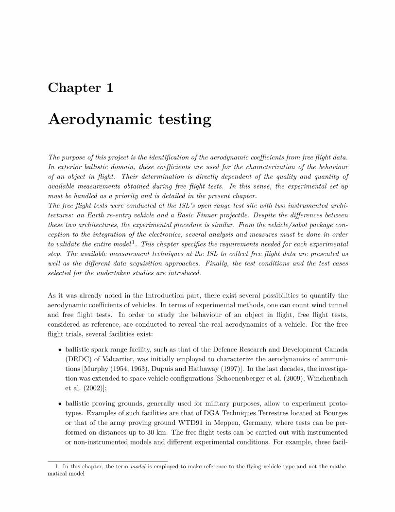
The purpose of this project is the identification of the aerodynamic coefficients from free flight data.In exterior ballistic domain, these coefficients are used for the characterization of the behaviourof an object in flight. Their determination is directly dependent of the quality and quantity ofavailable measurements obtained during free flight tests. In this sense, the experimental set-upmust be handled as a priority and is detailed in the present chapter.The free flight tests were conducted at the ISL’s open range test site with two instrumented archi-tectures: an Earth re-entry vehicle and a Basic Finner projectile. Despite the differences betweenthese two architectures, the experimental procedure is similar. From the vehicle/sabot package con-ception to the integration of the electronics, several analysis and measures must be done in orderto validate the entire model 1. This chapter specifies the requirements needed for each experimentalstep. The available measurement techniques at the ISL to collect free flight data are presented aswell as the different data acquisition approaches. Finally, the test conditions and the test casesselected for the undertaken studies are introduced.
As it was already noted in the Introduction part, there exist several possibilities to quantify theaerodynamic coefficients of vehicles. In terms of experimental methods, one can count wind tunneland free flight tests. In order to study the behaviour of an object in flight, free flight tests,considered as reference, are conducted to reveal the real aerodynamics of a vehicle. For the freeflight trials, several facilities exist:
• ballistic spark range facility, such as that of the Defence Research and Development Canada(DRDC) of Valcartier, was initially employed to characterize the aerodynamics of ammuni-tions [Murphy (1954, 1963), Dupuis and Hathaway (1997)]. In the last decades, the investiga-tion was extended to space vehicle configurations [Schoenenberger et al. (2009), Winchenbachet al. (2002)];
• ballistic proving grounds, generally used for military purposes, allow to experiment proto-types. Examples of such facilities are that of DGA Techniques Terrestres located at Bourgesor that of the army proving ground WTD91 in Meppen, Germany, where tests can be per-formed on distances up to 30 km. The free flight tests can be carried out with instrumentedor non-instrumented models and different experimental conditions. For example, these facil-
1. In this chapter, the term model is employed to make reference to the flying vehicle type and not the mathe-matical model
10 Chapter 1. Aerodynamic testing
ities enable to study trajectories at different elevations, over different distances, initial yaws,or velocities.
Before going further, it is important to introduce the notion of the Mach number, often used inthe field of exterior ballistic to express the velocity. It is a dimensionless quantity defined as theratio of the velocity V to the speed of sound a, as follows:
M = V/a (1.1)
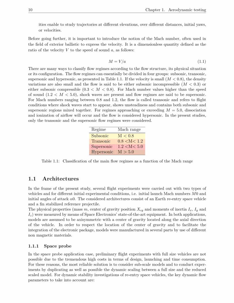
There are many ways to classify flow regimes according to the flow structure, its physical situationor its configuration. The flow regimes can essentially be divided in four groups: subsonic, transonic,supersonic and hypersonic, as presented in Table 1.1. If the velocity is small (M < 0.8), the densityvariations are also small and the flow is said to be either subsonic incompressible (M < 0.3) oreither subsonic compressible (0.3 < M < 0.8). For Mach number values higher than the speedof sound (1.2 < M < 5.0), shock waves are present and flow regimes are said to be supersonic.For Mach numbers ranging between 0.8 and 1.2, the flow is called transonic and refers to flightconditions where shock waves start to appear, shows unsteadiness and contains both subsonic andsupersonic regions mixed together. For regimes approaching or exceeding M = 5.0, dissociationand ionization of airflow will occur and the flow is considered hypersonic. In the present studies,only the transonic and the supersonic flow regimes were considered.
Regime Mach rangeSubsonic M < 0.8Transonic 0.8 <M< 1.2Supersonic 1.2 <M< 5.0Hypersonic M > 5.0
Table 1.1: Classification of the main flow regimes as a function of the Mach range
1.1 Architectures
In the frame of the present study, several flight experiments were carried out with two types ofvehicles and for different initial experimental conditions, i.e. initial launch Mach numbers M0 andinitial angles of attack α0. The considered architectures consist of an Earth re-entry space vehicleand a fin stabilized reference projectile.The physical properties (mass m, center of gravity position Xcg and moments of inertia Ix, Iy andIz) were measured by means of Space Electronics’ state-of-the-art equipment. In both applications,models are assumed to be axisymmetric with a center of gravity located along the axial directionof the vehicle. In order to respect the location of the center of gravity and to facilitate theintegration of the electronic package, models were manufactured in several parts by use of differentnon magnetic materials.
1.1.1 Space probe
In the space probe application case, preliminary flight experiments with full size vehicles are notpossible due to the tremendous high costs in terms of design, launching and time consumption.For these reasons, the most reliable solution is to consider sub-scale models and to conduct exper-iments by duplicating as well as possible the dynamic scaling between a full size and the reducedscaled model. For dynamic stability investigations of re-entry space vehicles, the key dynamic flowparameters to take into account are:
1.1. Architectures 11
• the Reynolds number: it is believed that similarity in terms of flow regime must be achieved,but once a turbulent flow regime is established, the Reynolds number dependency are believedto be minimal for such blunt bodies [Winchenbach et al. (2002)];
• the Mach number M : this parameter, easy to duplicate, is much more important since bluntbodies experience dynamic instabilities at a limited range of Mach number between 0.9 and3.0;
• the reduced spin rate : ωx = ωxd/2V , where ωx is the spin rate and d the vehicle diameter;
• the relative density parameter: m/ρd3, and the relative mass moment of inertia : md2/It,where ρ is the air density and It the transversal moment of inertia when the postulate ofIy = Iz is made. These two ratios are contained in the non-dimensionalized equations ofmotion for a decelerating vehicle [Berner et al. (2012)];
• the reduced frequency parameter f (RFP): this parameter involves the oscillation frequencyf which represents the ratio of a characteristic length of the model to the wave-length of theoscillation [Berner et al. (2009), Dobre et al. (2015)].
Consequently, the optimization of the parameters that allows duplicating flow and dynamic scaling,for characterizing the real vehicle in free flight, consists in:
• reducing model diameter to duplicate the Reynolds number,
• reducing the model diameter and increasing the model mass to duplicate the relative densityparameter,
• maximizing the transverse inertia moment to improve the reduced frequency, or increase thedensity. This last solution is not very convenient on ground facilities.
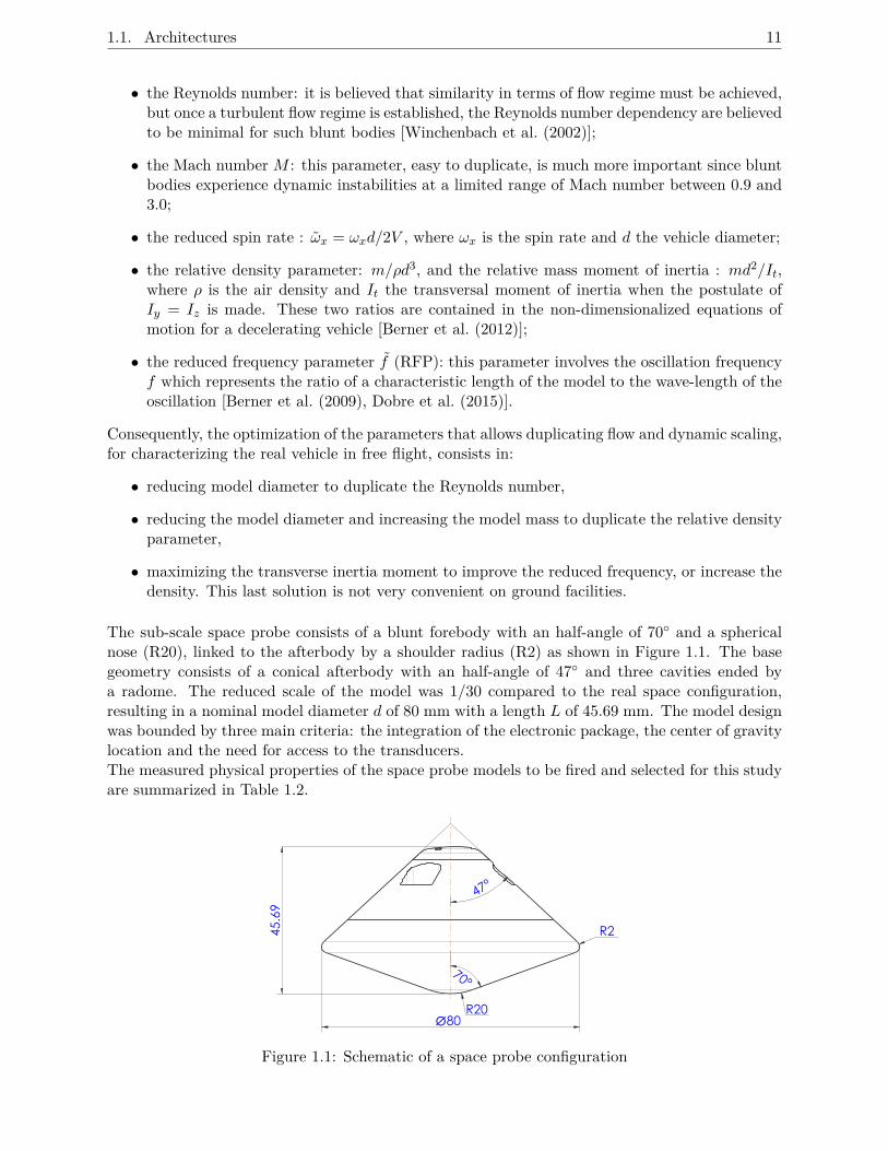
The sub-scale space probe consists of a blunt forebody with an half-angle of 70◦ and a sphericalnose (R20), linked to the afterbody by a shoulder radius (R2) as shown in Figure 1.1. The basegeometry consists of a conical afterbody with an half-angle of 47◦ and three cavities ended bya radome. The reduced scale of the model was 1/30 compared to the real space configuration,resulting in a nominal model diameter d of 80 mm with a length L of 45.69 mm. The model designwas bounded by three main criteria: the integration of the electronic package, the center of gravitylocation and the need for access to the transducers.The measured physical properties of the space probe models to be fired and selected for this studyare summarized in Table 1.2.
45.69
R2080∅
70°
47°
R2
Figure 1.1: Schematic of a space probe configuration
12 Chapter 1. Aerodynamic testing
Model d L m Xcg/nose Xcg/d Ix Iy Iz
# (mm) (mm) (g) (mm) (%) (kg.m2) (kg.m2) (kg.m2)A1 80.02 45.74 1246.9 21.22 26.52 7.6918 · 10−4 4.8267 · 10−4 4.8206 · 10−4
B1 80.07 45.75 1246 21.21 26.49 7.7057 · 10−4 4.8367 · 10−4 4.8311 · 10−4
C1 80.01 45.71 1243.9 21.24 26.55 7.6810 · 10−4 4.8121 · 10−4 4.8121 · 10−4
D1 80.00 45.8 1233.3 21.13 26.41 7.6269 · 10−4 4.7398 · 10−4 4.7377 · 10−4
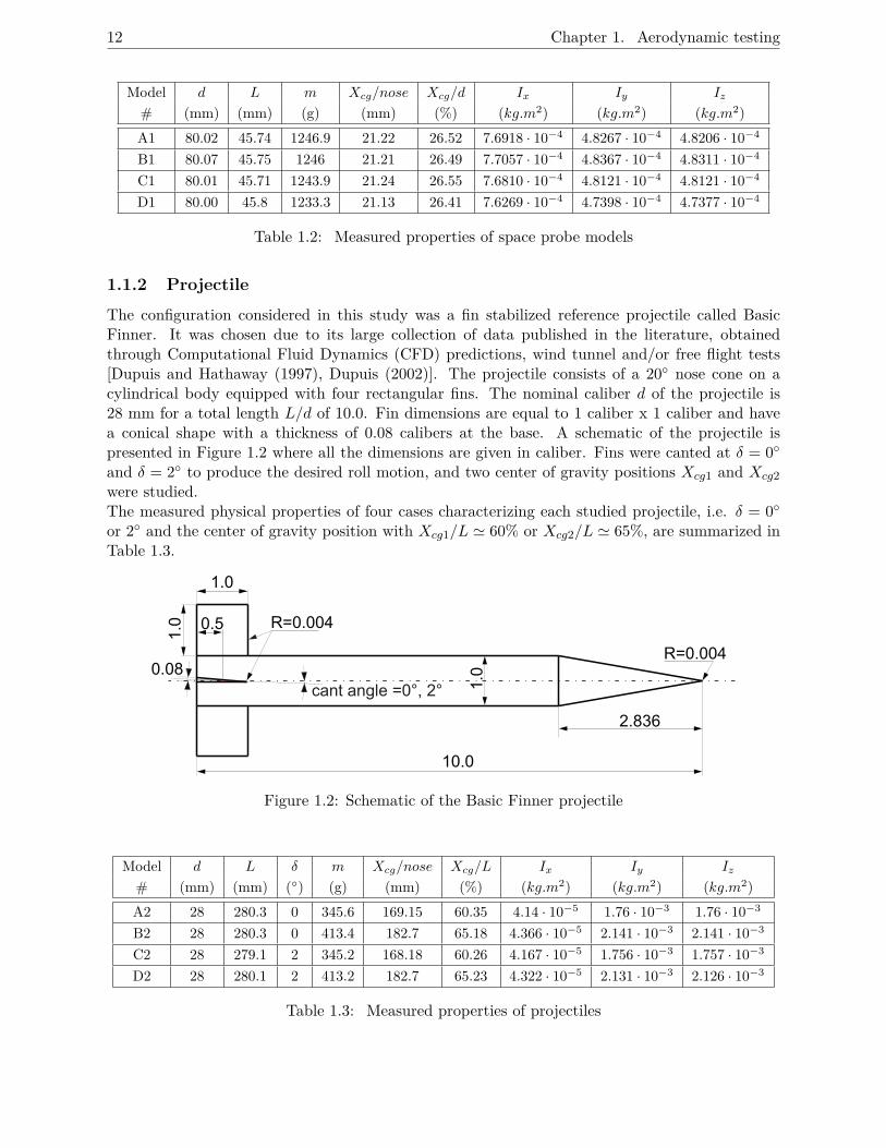
Table 1.2: Measured properties of space probe models
1.1.2 Projectile
The configuration considered in this study was a fin stabilized reference projectile called BasicFinner. It was chosen due to its large collection of data published in the literature, obtainedthrough Computational Fluid Dynamics (CFD) predictions, wind tunnel and/or free flight tests[Dupuis and Hathaway (1997), Dupuis (2002)]. The projectile consists of a 20◦ nose cone on acylindrical body equipped with four rectangular fins. The nominal caliber d of the projectile is28 mm for a total length L/d of 10.0. Fin dimensions are equal to 1 caliber x 1 caliber and havea conical shape with a thickness of 0.08 calibers at the base. A schematic of the projectile ispresented in Figure 1.2 where all the dimensions are given in caliber. Fins were canted at δ = 0◦and δ = 2◦ to produce the desired roll motion, and two center of gravity positions Xcg1 and Xcg2were studied.The measured physical properties of four cases characterizing each studied projectile, i.e. δ = 0◦or 2◦ and the center of gravity position with Xcg1/L ' 60% or Xcg2/L ' 65%, are summarized inTable 1.3.
1.0
1.0
10.0
2.836
1.0
R=0.004
R=0.004
0.5
0.08cant angle =0°, 2°
Figure 1.2: Schematic of the Basic Finner projectile
Model d L δ m Xcg/nose Xcg/L Ix Iy Iz
# (mm) (mm) (◦) (g) (mm) (%) (kg.m2) (kg.m2) (kg.m2)A2 28 280.3 0 345.6 169.15 60.35 4.14 · 10−5 1.76 · 10−3 1.76 · 10−3
B2 28 280.3 0 413.4 182.7 65.18 4.366 · 10−5 2.141 · 10−3 2.141 · 10−3
C2 28 279.1 2 345.2 168.18 60.26 4.167 · 10−5 1.756 · 10−3 1.757 · 10−3
D2 28 280.1 2 413.2 182.7 65.23 4.322 · 10−5 2.131 · 10−3 2.126 · 10−3
Table 1.3: Measured properties of projectiles
1.2. Sabot design 13
1.2 Sabot design
Since the sub caliber models have to be launched from a smooth bore powdered gun, special sabotswere designed at different initial angles of attack α0. The initial angle of attack characterizes theorientation of the model into the sabot before firing 2. For the sabot separation without highinitial disturbances, the main aspects to consider for the sabot design are the model geometry,the total mass, the muzzle velocity and the gun acceleration. Some of the aspects like separation,acceleration and velocity have to be consistent from one trial to another.
1.2.1 Space probe
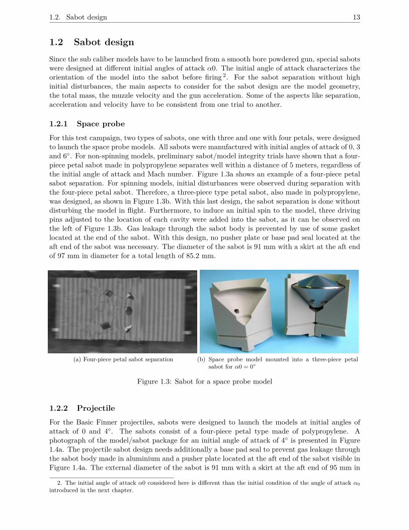
For this test campaign, two types of sabots, one with three and one with four petals, were designedto launch the space probe models. All sabots were manufactured with initial angles of attack of 0, 3and 6◦. For non-spinning models, preliminary sabot/model integrity trials have shown that a four-piece petal sabot made in polypropylene separates well within a distance of 5 meters, regardless ofthe initial angle of attack and Mach number. Figure 1.3a shows an example of a four-piece petalsabot separation. For spinning models, initial disturbances were observed during separation withthe four-piece petal sabot. Therefore, a three-piece type petal sabot, also made in polypropylene,was designed, as shown in Figure 1.3b. With this last design, the sabot separation is done withoutdisturbing the model in flight. Furthermore, to induce an initial spin to the model, three drivingpins adjusted to the location of each cavity were added into the sabot, as it can be observed onthe left of Figure 1.3b. Gas leakage through the sabot body is prevented by use of some gasketlocated at the end of the sabot. With this design, no pusher plate or base pad seal located at theaft end of the sabot was necessary. The diameter of the sabot is 91 mm with a skirt at the aft endof 97 mm in diameter for a total length of 85.2 mm.
(a) Four-piece petal sabot separation
(b) Space probe model mounted into a three-piece petalsabot for α0 = 0◦
Figure 1.3: Sabot for a space probe model
1.2.2 Projectile
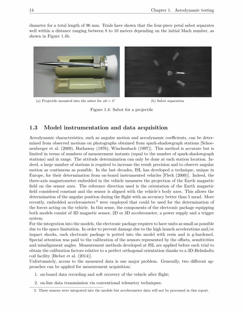
For the Basic Finner projectiles, sabots were designed to launch the models at initial angles ofattack of 0 and 4◦. The sabots consist of a four-piece petal type made of polypropylene. Aphotograph of the model/sabot package for an initial angle of attack of 4◦ is presented in Figure1.4a. The projectile sabot design needs additionally a base pad seal to prevent gas leakage throughthe sabot body made in aluminium and a pusher plate located at the aft end of the sabot visible inFigure 1.4a. The external diameter of the sabot is 91 mm with a skirt at the aft end of 95 mm in
2. The initial angle of attack α0 considered here is different than the initial condition of the angle of attack α0introduced in the next chapter.
14 Chapter 1. Aerodynamic testing
diameter for a total length of 96 mm. Trials have shown that the four-piece petal sabot separateswell within a distance ranging between 8 to 10 meters depending on the initial Mach number, asshown in Figure 1.4b.
(a) Projectile mounted into the sabot for α0 = 4◦ (b) Sabot separation
Figure 1.4: Sabot for a projectile
1.3 Model instrumentation and data acquisition
Aerodynamic characteristics, such as angular motion and aerodynamic coefficients, can be deter-mined from observed motions on photographs obtained from spark-shadowgraph stations [Schoe-nenberger et al. (2009), Hathaway (1976), Winchenbach (1997)]. This method is accurate but islimited in terms of numbers of measurement instants (equal to the number of spark-shadowgraphstations) and in range. The attitude determination can only be done at each station location. In-deed, a large number of stations is required to increase the result precision and to observe angularmotion as continuous as possible. In the last decades, ISL has developed a technique, unique inEurope, for their determination from on-board instrumented vehicles [Fleck (2000)]. Indeed, thethree-axis magnetometer embedded in the vehicle measures the projection of the Earth magneticfield on the sensor axes. The reference direction used is the orientation of the Earth magneticfield considered constant and the sensor is aligned with the vehicle’s body axes. This allows thedetermination of the angular position during the flight with an accuracy better than 5 mrad. Morerecently, embedded accelerometers 3 were employed that could be used for the determination ofthe forces acting on the vehicle. In this sense, the components of the electronic package equippingboth models consist of 3D magnetic sensor, 2D or 3D accelerometer, a power supply and a triggersystem.For the integration into the models, the electronic package requires to have units as small as possibledue to the space limitation. In order to prevent damage due to the high launch accelerations and/orimpact shocks, each electronic package is potted into the model with resin and is g-hardened.Special attention was paid to the calibration of the sensors represented by the offsets, sensitivitiesand misalignment angles. Measurement methods developed at ISL are applied before each trial toobtain the calibration factors relative to a perfect orthogonal orientation thanks to a 3D-Helmholtzcoil facility [Bieber et al. (2014)].Unfortunately, access to the measured data is one major problem. Generally, two different ap-proaches can be applied for measurement acquisition:
1. on-board data recording and soft recovery of the vehicle after flight;
2. on-line data transmission via conventional telemetry techniques.3. These sensors were integrated into the models but accelerometer data will not be processed in this report.
1.3. Model instrumentation and data acquisition 15
1.3.1 Space probe
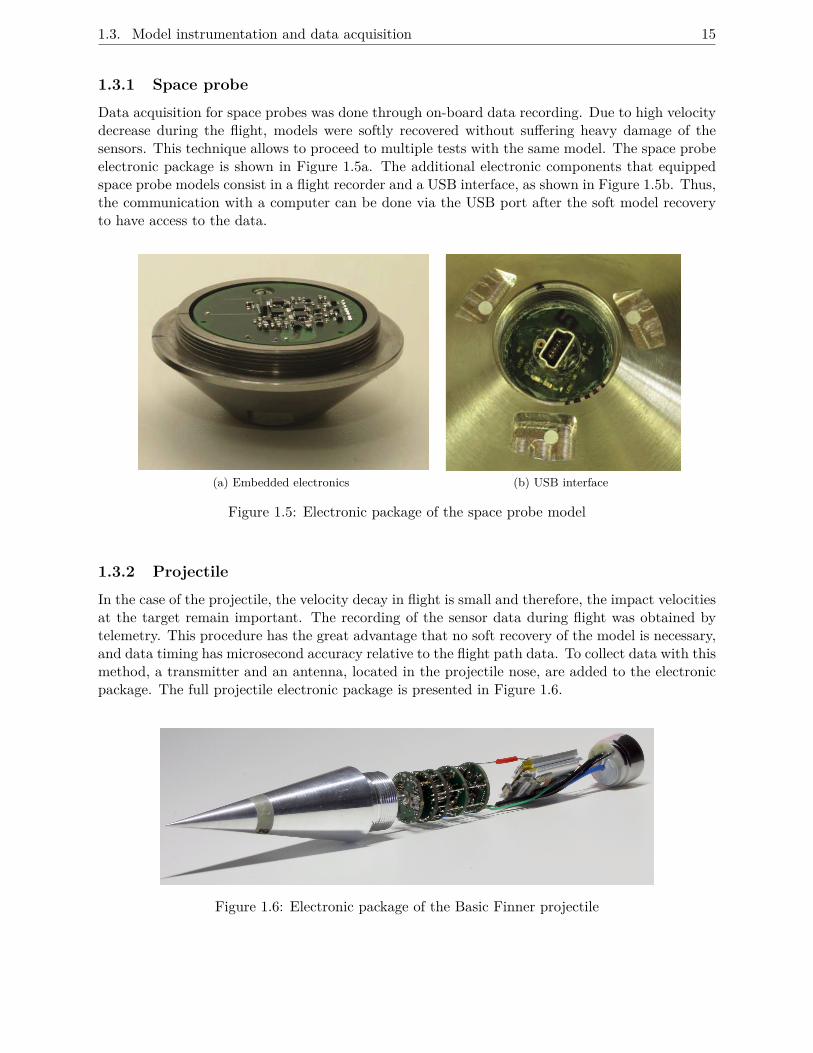
Data acquisition for space probes was done through on-board data recording. Due to high velocitydecrease during the flight, models were softly recovered without suffering heavy damage of thesensors. This technique allows to proceed to multiple tests with the same model. The space probeelectronic package is shown in Figure 1.5a. The additional electronic components that equippedspace probe models consist in a flight recorder and a USB interface, as shown in Figure 1.5b. Thus,the communication with a computer can be done via the USB port after the soft model recoveryto have access to the data.
(a) Embedded electronics (b) USB interface
Figure 1.5: Electronic package of the space probe model
1.3.2 Projectile
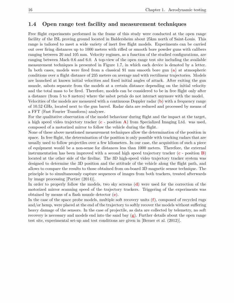
In the case of the projectile, the velocity decay in flight is small and therefore, the impact velocitiesat the target remain important. The recording of the sensor data during flight was obtained bytelemetry. This procedure has the great advantage that no soft recovery of the model is necessary,and data timing has microsecond accuracy relative to the flight path data. To collect data with thismethod, a transmitter and an antenna, located in the projectile nose, are added to the electronicpackage. The full projectile electronic package is presented in Figure 1.6.
Figure 1.6: Electronic package of the Basic Finner projectile
16 Chapter 1. Aerodynamic testing
1.4 Open range test facility and measurement techniques
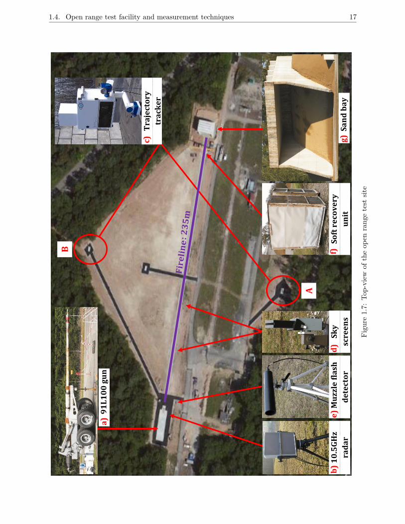
Free flight experiments performed in the frame of this study were conducted at the open rangefacility of the ISL proving ground located in Baldersheim about 25km north of Saint-Louis. Thisrange is tailored to meet a wide variety of inert free flight models. Experiments can be carriedout over firing distances up to 1000 meters with rifled or smooth bore powder guns with calibersranging between 20 and 105 mm. Velocity regimes, as a function of the studied configurations, areranging between Mach 0.6 and 6.0. A top-view of the open range test site including the availablemeasurement techniques is presented in Figure 1.7, in which each device is denoted by a letter.In both cases, models were fired from a classical 91 mm smooth bore gun (a) at atmosphericconditions over a flight distance of 235 meters on average and with rectilinear trajectories. Modelsare launched at known initial velocities and fixed initial angles of attack. After exiting the gunmuzzle, sabots separate from the models at a certain distance depending on the initial velocityand the total mass to be fired. Therefore, models can be considered to be in free flight only aftera distance (from 5 to 8 meters) where the sabot petals do not interact anymore with the model.Velocities of the models are measured with a continuous Doppler radar (b) with a frequency rangeof 10.52 GHz, located next to the gun barrel. Radar data are reduced and processed by means ofa FFT (Fast Fourier Transform) analyzer.For the qualitative observation of the model behaviour during flight and the impact at the target,a high speed video trajectory tracker (c - position A) from Specialized Imaging Ltd. was used,composed of a motorized mirror to follow the vehicle during the flight.None of these above mentioned measurement techniques allow the determination of the position inspace. In free flight, the determination of the position is only possible with tracking radars that areusually used to follow projectiles over a few kilometers. In our case, the acquisition of such a pieceof equipment would be a non-sense for distances less than 1000 meters. Therefore, the externalinstrumentation has been improved with a second high speed trajectory tracker (c - position B)located at the other side of the fireline. The 3D high-speed video trajectory tracker system wasdesigned to determine the 3D position and the attitude of the vehicle along the flight path, andallows to compare the results to those obtained from on-board 3D magnetic sensor technique. Theprinciple is to simultaneously capture sequences of images from both trackers, treated afterwardsby image processing [Portier (2014)].In order to properly follow the models, two sky screens (d) were used for the correction of themotorized mirror scanning speed of the trajectory trackers. Triggering of the experiments wasobtained by means of a flash muzzle detector (e).In the case of the space probe models, multiple soft recovery units (f), composed of recycled rugsand/or hemp, were placed at the end of the trajectory to softly recover the models without sufferingheavy damage of the sensors. In the case of projectile, as data are collected by telemetry, no softrecovery is necessary and models end into the sand bay (g). Further details about the open rangetest site, experimental set-up and test conditions are given in [Berner et al. (2012)].
1.4. Open range test facility and measurement techniques 17
a)
91
L1
00
gu
n
S
an
d b
ay
M
uzz
le f
lash
de
tect
or
10
.5G
Hz
rad
ar
Sk
y
scre
en
s
Tra
ject
ory
tra
cke
r
So
ft r
eco
ve
ry
un
it
b)
c)
d)
e
)
f)
g)
A
B
Figu
re1.
7:To
p-vi
ewof
the
open
rang
ete
stsit
e
18 Chapter 1. Aerodynamic testing
1.5 Test conditions
Free flight experiments were carried out for electronically instrumented configurations. Only twocriteria define the constraints imposed by the experimental conditions, the initial Mach numberM0 and initial angle of attack α0.
1.5.1 Space probe
Within the context of a third party contract with ESA (European Space Agency), two test cam-paigns were conducted with a space probe at different initial Mach numbers M0 ranging between2.0 and 3.0, for initial angles of attack α0 of 0, 3 and 6◦ and for two different center of gravitypositions Xcg1 and Xcg2. For this study, five non-contractual spinning free flight tests having thesame center of gravity position Xcg1 were selected and are summarized in Table 1.4. The corre-sponding models used for each test case are specified in the test matrix. Due to the soft recovery,the model #B1 was fired twice which explains why the same model was used for test cases 2 and3.
M0 = 2.0 M0 = 3.0test case 1 (model #A1) test case 4 (model #C1)
α0 = 0◦test case 2 (model #B1) test case 5 (model #D1)
α0 = 3◦ test case 3 (model #B1)
Table 1.4: Test matrix for the space probe models
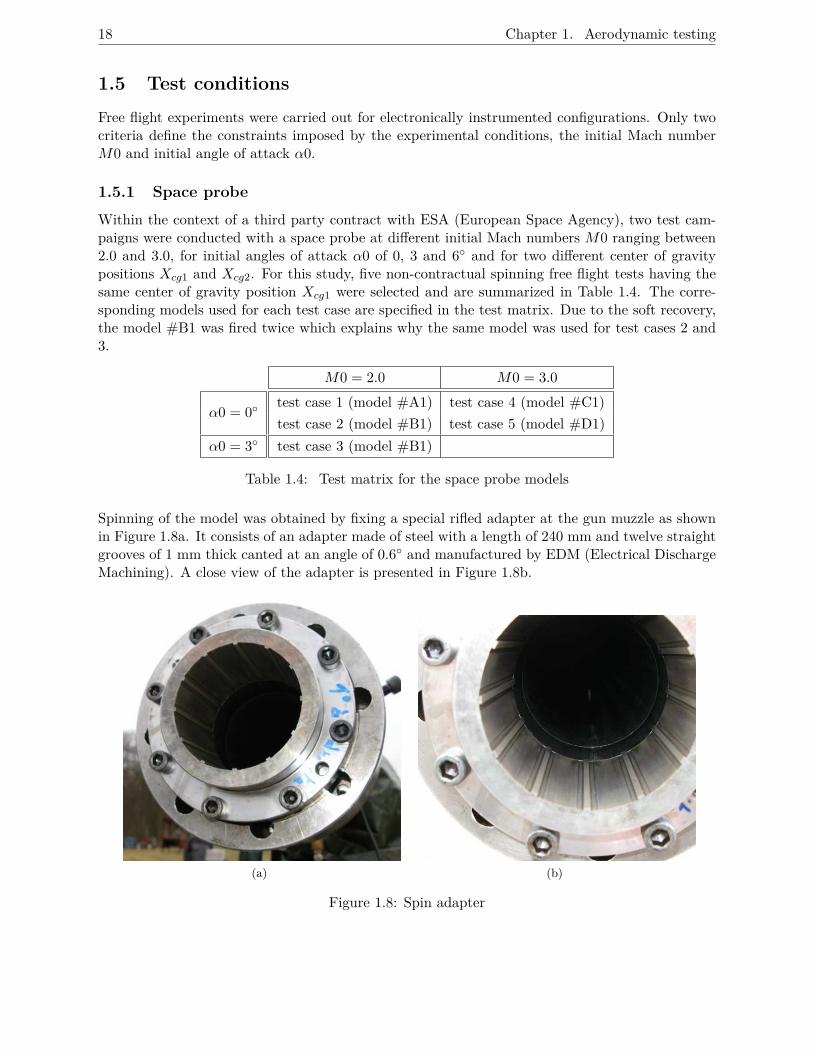
Spinning of the model was obtained by fixing a special rifled adapter at the gun muzzle as shownin Figure 1.8a. It consists of an adapter made of steel with a length of 240 mm and twelve straightgrooves of 1 mm thick canted at an angle of 0.6◦ and manufactured by EDM (Electrical DischargeMachining). A close view of the adapter is presented in Figure 1.8b.
(a) (b)
Figure 1.8: Spin adapter
1.6. Concluding remarks 19
1.5.2 Projectile
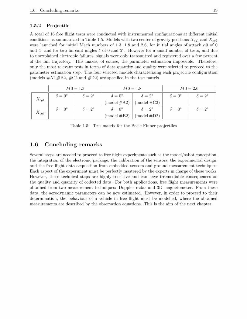
A total of 16 free flight tests were conducted with instrumented configurations at different initialconditions as summarized in Table 1.5. Models with two center of gravity positions Xcg1 and Xcg2were launched for initial Mach numbers of 1.3, 1.8 and 2.6, for initial angles of attack α0 of 0and 4◦ and for two fin cant angles δ of 0 and 2◦. However for a small number of tests, and dueto unexplained electronic failures, signals were only transmitted and registered over a few percentof the full trajectory. This makes, of course, the parameter estimation impossible. Therefore,only the most relevant tests in terms of data quantity and quality were selected to proceed to theparameter estimation step. The four selected models characterizing each projectile configuration(models #A2,#B2, #C2 and #D2) are specified in the test matrix.
M0 = 1.3 M0 = 1.8 M0 = 2.6δ = 0◦ δ = 2◦ δ = 0◦ δ = 2◦ δ = 0◦ δ = 2◦
Xcg1 (model #A2) (model #C2)δ = 0◦ δ = 2◦ δ = 0◦ δ = 2◦ δ = 0◦ δ = 2◦
Xcg2 (model #B2) (model #D2)
Table 1.5: Test matrix for the Basic Finner projectiles
1.6 Concluding remarks
Several steps are needed to proceed to free flight experiments such as the model/sabot conception,the integration of the electronic package, the calibration of the sensors, the experimental design,and the free flight data acquisition from embedded sensors and ground measurement techniques.Each aspect of the experiment must be perfectly mastered by the experts in charge of these works.However, these technical steps are highly sensitive and can have irremediable consequences onthe quality and quantity of collected data. For both applications, free flight measurements wereobtained from two measurement techniques: Doppler radar and 3D magnetometer. From thesedata, the aerodynamic parameters can be now estimated. However, in order to proceed to theirdetermination, the behaviour of a vehicle in free flight must be modelled, where the obtainedmeasurements are described by the observation equations. This is the aim of the next chapter.

20 Chapter 1. Aerodynamic testing
Chapter 2
Modelling of a vehicle in free flight
Experiments make it possible to access the data obtained by means of different measurement tech-niques. This data is essential to conduct parameter estimation. In order to reach this objective,an identification procedure composed of several steps must be defined. This chapter presents thefirst step of the proposed aerodynamic coefficient identification procedure, the physical modelling,namely the construction of mathematical models of dynamical systems. To have a physical in-terpretation of the state variables, the model describing the behaviour of a vehicle in free flight isconstructed based on Newton’s and Euler’s laws. This mathematical model includes both the vehicleequations of motion and the aerodynamic coefficient descriptions. The state equations are formu-lated as ordinary differential equations and observation equations for the measured outputs. It is anonlinear state-space model composed of 12 state equations and 4 output measurement equations.The equations of motion are valid for several types of vehicle in flight like space probes, UnmannedAerial Vehicles, ammunition or airplane, and depend on the considered coordinate frame. Further-more, it is assumed that the vehicle is a rigid body. The proposed aerodynamic coefficient modelequations are described using polynomials and polynomial splines with time-invariant parameters,which are precisely the parameters to be estimated, and depend on several state variables. Thepresented aerodynamic model is valid only for space probe and ammunition architectures.
2.1 Coordinate systems
Before developing the vehicle equations of motion, a description of the coordinate systems andsign conventions is mandatory. All these reference frames are right handed and have orthogonalaxes. Generally, three main frames are taken into account:
• Earth frame OxE ,yE ,zE , commonly used to determine the vehicle motion with respect to(w.r.t.) fixed axes, is defined about the Earth. Its origin is an arbitrary point on the Earthsurface, where the positive OxE axis points toward the geographic North, the positive OyEaxis points to the East, and the positive OzE axis points to the center of the Earth.
• Body frame Ox,y,z is fixed w.r.t. the studied vehicle and is moving with it. The originof this reference frame is situated at the vehicle center of gravity, with positive Ox pointingdownrange through the vehicle nose, positive Oy axis in the horizontal plane and pointingto the right looking downrange, and positive Oz axis pointing down w.r.t. the body. In thisstudy it can be assumed that Oxz plane is a plane of symmetry of the vehicle.
• Wind frame OxW ,yW ,zW , also called aerodynamic or stability frame, is relative to the vehicletrajectory through the air. Its origin is located at the vehicle center of gravity, with positive
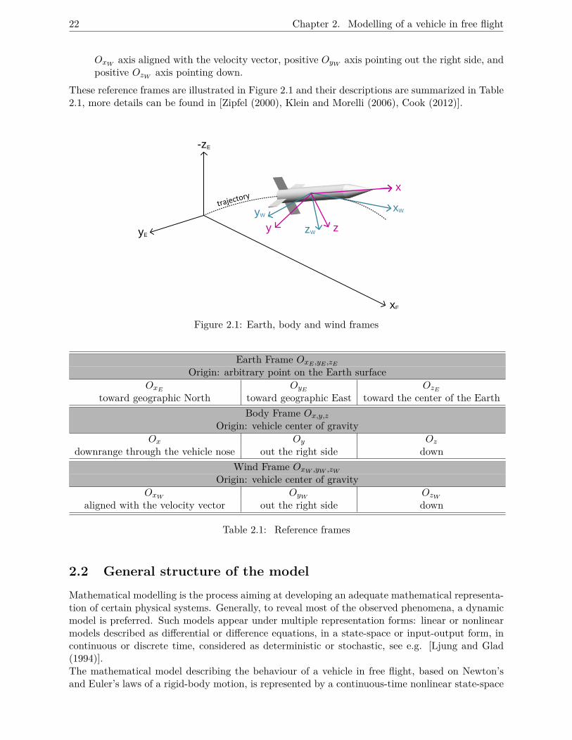
22 Chapter 2. Modelling of a vehicle in free flight
OxW axis aligned with the velocity vector, positive OyW axis pointing out the right side, andpositive OzW axis pointing down.
These reference frames are illustrated in Figure 2.1 and their descriptions are summarized in Table2.1, more details can be found in [Zipfel (2000), Klein and Morelli (2006), Cook (2012)].
x
zy
xWyW
zW
xE
yE
-zE
trajectory
Figure 2.1: Earth, body and wind frames
Earth Frame OxE ,yE ,zEOrigin: arbitrary point on the Earth surface
OxE OyE OzEtoward geographic North toward geographic East toward the center of the Earth
Body Frame Ox,y,zOrigin: vehicle center of gravity
Ox Oy Ozdownrange through the vehicle nose out the right side down
Wind Frame OxW ,yW ,zW
Origin: vehicle center of gravityOxW OyW OzW
aligned with the velocity vector out the right side down
Table 2.1: Reference frames
2.2 General structure of the model
Mathematical modelling is the process aiming at developing an adequate mathematical representa-tion of certain physical systems. Generally, to reveal most of the observed phenomena, a dynamicmodel is preferred. Such models appear under multiple representation forms: linear or nonlinearmodels described as differential or difference equations, in a state-space or input-output form, incontinuous or discrete time, considered as deterministic or stochastic, see e.g. [Ljung and Glad(1994)].The mathematical model describing the behaviour of a vehicle in free flight, based on Newton’sand Euler’s laws of a rigid-body motion, is represented by a continuous-time nonlinear state-space
2.3. State equations 23
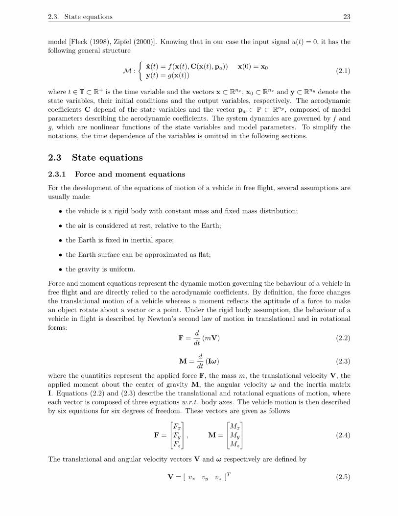
model [Fleck (1998), Zipfel (2000)]. Knowing that in our case the input signal u(t) = 0, it has thefollowing general structure
M :{
x(t) = f(x(t),C(x(t),pa)) x(0) = x0y(t) = g(x(t)) (2.1)
where t ∈ T ⊂ R+ is the time variable and the vectors x ⊂ Rnx , x0 ⊂ Rnx and y ⊂ Rny denote thestate variables, their initial conditions and the output variables, respectively. The aerodynamiccoefficients C depend of the state variables and the vector pa ∈ P ⊂ Rnp , composed of modelparameters describing the aerodynamic coefficients. The system dynamics are governed by f andg, which are nonlinear functions of the state variables and model parameters. To simplify thenotations, the time dependence of the variables is omitted in the following sections.
2.3 State equations
2.3.1 Force and moment equations
For the development of the equations of motion of a vehicle in free flight, several assumptions areusually made:
• the vehicle is a rigid body with constant mass and fixed mass distribution;
• the air is considered at rest, relative to the Earth;
• the Earth is fixed in inertial space;
• the Earth surface can be approximated as flat;
• the gravity is uniform.
Force and moment equations represent the dynamic motion governing the behaviour of a vehicle infree flight and are directly relied to the aerodynamic coefficients. By definition, the force changesthe translational motion of a vehicle whereas a moment reflects the aptitude of a force to makean object rotate about a vector or a point. Under the rigid body assumption, the behaviour of avehicle in flight is described by Newton’s second law of motion in translational and in rotationalforms:
F = d
dt(mV) (2.2)
M = d
dt(Iω) (2.3)
where the quantities represent the applied force F, the mass m, the translational velocity V, theapplied moment about the center of gravity M, the angular velocity ω and the inertia matrixI. Equations (2.2) and (2.3) describe the translational and rotational equations of motion, whereeach vector is composed of three equations w.r.t. body axes. The vehicle motion is then describedby six equations for six degrees of freedom. These vectors are given as follows
F =
FxFyFz
, M =
Mx
My
Mz
(2.4)
The translational and angular velocity vectors V and ω respectively are defined by
V = [ vx vy vz ]T (2.5)

24 Chapter 2. Modelling of a vehicle in free flight
ω = [ ωx ωy ωz ]T (2.6)
and their components are represented in Figure 2.2 in body axes.
α
β
V
ωx x
z
y
ωy
ωz
αt
vx
vzvy
Figure 2.2: Representation of state variables of a space probe model
An assumption often used is that the inertia matrix I is considered to be diagonal 1. The consideredinertia matrix is then
I =
Ix 0 00 Iy 00 0 Iz
(2.7)
where Ix, Iy and Iz are the longitudinal and lateral moments of inertia.Equations (2.2) and (2.3) are valid in an Earth reference frame. However, it is generally recom-mended to express the variables of both previous equations in a body reference frame, which willtranslate and rotate relative to the Earth frame. For rotating body axes system, the derivativeoperator considered the rate of change of the vector components expressed in the body frame andthe axis system rotation, formulate by the following equation:
d
dt(.) = δ
δt(.) + ω × (.) (2.8)
By considering equations (2.2), (2.3) and (2.8), the force and moment equations in body axes aredescribed by
F = mV + ω ×mV (2.9)
M = Iω + ω × Iω (2.10)
The applied forces and moments contain aerodynamic, thrust and gravity components. In thisapplication, the absence of propulsion allows to set the thrust force and moment to zero. Moreover,due to the rigid-body assumption made on the uniformity of the gravity applied through the vehiclecenter of gravity, there is no gravity moment acting on the vehicle. Consequently, the forces andmoments equations can be written as
FA + FG = mV + ω ×mV (2.11)
MA = Iω + ω × Iω (2.12)
1. For the model description with the complete inertia matrix, see e.g. [Klein and Morelli (2006)].
2.3. State equations 25
where FA and FG represent the aerodynamic and gravity forces respectively, and MA the aerody-namic moment. These vectors are defined as
FA = qS
CXCYCZ
B
, FG = m
−g sin θg sinφ cos θg cosφ cos θ
B
(2.13)
MA = qSd
ClCmCn
B
(2.14)
where the physical properties are the reference diameter d, the reference surface area S = (πd2)/4and the dynamic pressure q = 1
2ρV2, where ρ represents the air density. The global force and
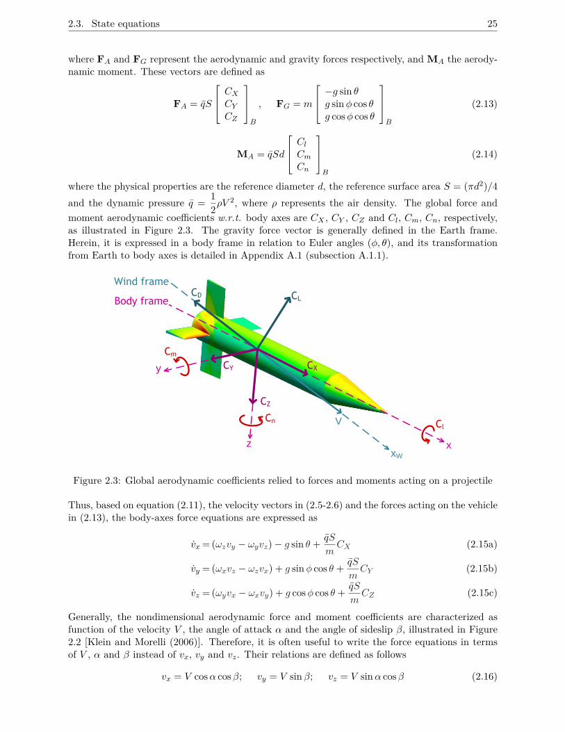
moment aerodynamic coefficients w.r.t. body axes are CX , CY , CZ and Cl, Cm, Cn, respectively,as illustrated in Figure 2.3. The gravity force vector is generally defined in the Earth frame.Herein, it is expressed in a body frame in relation to Euler angles (φ, θ), and its transformationfrom Earth to body axes is detailed in Appendix A.1 (subsection A.1.1).
xW
Wind frame
Body frame
V
CD CL
CX
Cm
x
y
CZ
CY
ClCn
z
Figure 2.3: Global aerodynamic coefficients relied to forces and moments acting on a projectile
Thus, based on equation (2.11), the velocity vectors in (2.5-2.6) and the forces acting on the vehiclein (2.13), the body-axes force equations are expressed as
vx = (ωzvy − ωyvz)− g sin θ + qS
mCX (2.15a)
vy = (ωxvz − ωzvx) + g sinφ cos θ + qS
mCY (2.15b)
vz = (ωyvx − ωxvy) + g cosφ cos θ + qS
mCZ (2.15c)
Generally, the nondimensional aerodynamic force and moment coefficients are characterized asfunction of the velocity V , the angle of attack α and the angle of sideslip β, illustrated in Figure2.2 [Klein and Morelli (2006)]. Therefore, it is often useful to write the force equations in termsof V , α and β instead of vx, vy and vz. Their relations are defined as follows
vx = V cosα cosβ; vy = V sin β; vz = V sinα cosβ (2.16)
26 Chapter 2. Modelling of a vehicle in free flight
and the reverse transformations
V =√v2x + v2
y + v2z ; α = arctan(vz/vx); β = arcsin(vy/V ) (2.17)
The wind axis force equations are obtained by differentiating w.r.t. time the equations (2.17)
V = vxvx + vyvy + vz vzV
(2.18a)
α = vxvz − vz vxv2x + v2
z
(2.18b)
β = −vxvyvx + (v2x + v2
z)vy − vyvz vzV 2√v2x + v2
z
(2.18c)
The above equations can be transformed, by replacing vx, vy, vz by the relations in (2.16) andvx, vy, vz by the body force equations in (2.15). The force equations in wind axes are finallydescribed as
V = − qS
mCD + g(cos θ cosφ sinα cosβ + cos θ sinφ sin β − sin θ cosα cosβ) (2.19a)
α = − qS
mV cosβCL + ωy − tan β(ωx cosα+ ωz sinα) + g
V cosβ (cos θ cosφ cosα+ sin θ sinα)
(2.19b)
β = qS
mVCY w + ωx sinα− ωz cosα+ g
V(cos θ sinφ cosβ + sin θ cosα sin β − cosφ cos θ sinα sin β)
(2.19c)
where
CD =−CX cosα cosβ − CY sin β − CZ sinα cosβ (2.20a)CL = CX sinα− CZ cosα (2.20b)CY w=−CX cosα sin β + CY cosβ − CZ sinα sin β (2.20c)
represent the drag, the lift and the sideforce coefficients along the wind axes, respectively. Thedrag and the lift coefficients acting on a projectile are represented in Figure 2.3.In an equivalent manner, based on equation (2.12), on the angular velocity vector in (2.6), onthe aerodynamic moment vector in (2.14) and on the inertia matrix defined in (2.7), the momentequations are expressed as
ωx= 1Ix
(qSdCl − ωyωz(Iz − Iy)) (2.21a)
ωy= 1Iy
(qSdCm − ωxωz(Ix − Iz)) (2.21b)
ωz= 1Iz
(qSdCn − ωxωy(Iy − Ix)) (2.21c)
The force and moment equations depend on several physical properties like the mass of the vehiclem, the reference diameter d, the reference surface area S, the longitudinal and lateral momentsof inertia Ix, Iy and Iz and the gravitational acceleration g. These quantities are measured withgood accuracy before the experiment.
2.3. State equations 27
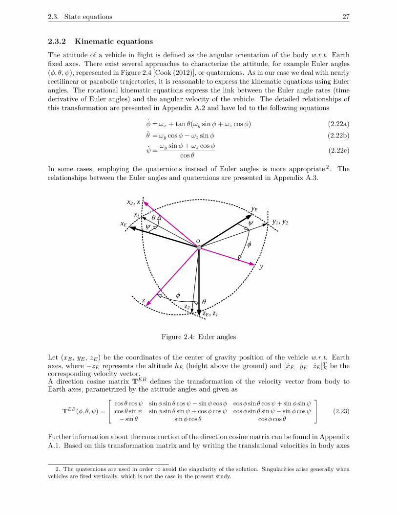
2.3.2 Kinematic equations
The attitude of a vehicle in flight is defined as the angular orientation of the body w.r.t. Earthfixed axes. There exist several approaches to characterize the attitude, for example Euler angles(φ, θ, ψ), represented in Figure 2.4 [Cook (2012)], or quaternions. As in our case we deal with nearlyrectilinear or parabolic trajectories, it is reasonable to express the kinematic equations using Eulerangles. The rotational kinematic equations express the link between the Euler angle rates (timederivative of Euler angles) and the angular velocity of the vehicle. The detailed relationships ofthis transformation are presented in Appendix A.2 and have led to the following equations
φ =ωx + tan θ(ωy sinφ+ ωz cosφ) (2.22a)θ =ωy cosφ− ωz sinφ (2.22b)
ψ= ωy sinφ+ ωz cosφcos θ (2.22c)
In some cases, employing the quaternions instead of Euler angles is more appropriate 2. Therelationships between the Euler angles and quaternions are presented in Appendix A.3.
O
q
y
f
xE
x1
x2 , xyE
y1 , y2
y
zz2
zE , z1
q
f
y
Figure 2.4: Euler angles
Let (xE , yE , zE) be the coordinates of the center of gravity position of the vehicle w.r.t. Earthaxes, where −zE represents the altitude hE (height above the ground) and [xE yE zE ]TE be thecorresponding velocity vector.A direction cosine matrix TEB defines the transformation of the velocity vector from body toEarth axes, parametrized by the attitude angles and given as
TEB(φ, θ, ψ) =
cos θ cosψ sinφ sin θ cosψ − sinψ cosφ cosφ sin θ cosψ + sinφ sinψcos θ sinψ sinφ sin θ sinψ + cosφ cosψ cosφ sin θ sinψ − sinφ cosψ− sin θ sinφ cos θ cosφ cos θ
(2.23)
Further information about the construction of the direction cosine matrix can be found in AppendixA.1. Based on this transformation matrix and by writing the translational velocities in body axes
2. The quaternions are used in order to avoid the singularity of the solution. Singularities arise generally whenvehicles are fired vertically, which is not the case in the present study.
28 Chapter 2. Modelling of a vehicle in free flight
as in equations (2.16), the translational kinematic equations can be written as xEyEzE
E
= TEB(ψ, θ, φ) ·
V cosα cosβV sin β
V sinα cosβ
B
and the resulting equations are,
xE =V cosα cosβ cos θ cosψ + V sin β(sinφ sin θ cosψ − cosφ sinψ)+V sinα cosβ(cosφ sin θ cosψ + sinφ sinψ) (2.24a)
yE =V cosα cosβ cos θ sinψ + V sin β(sinφ sin θ sinψ + cosφ cosψ)+V sinα cosβ(cosφ sin θ sinψ − sinφ cosψ) (2.24b)
zE = − V cosα cosβ sin θ + V sin β sinφ cos θ + V sinα cosβ cosφ cos θ (2.24c)
2.4 Aerodynamic coefficients
In the case of a vehicle in flight, its behaviour is directly influenced by initial and exterior con-ditions, such as temperature, pressure, presence of wind, as well as the physical properties of thebody (in terms of mass, center of gravity and inertia). All these conditions have an effect onthe aerodynamic coefficients. The importance of estimating them lies in the representation ofaerodynamic characteristics of a vehicle. Aerodynamic coefficients are the parameters describingand connecting forces and moments acting on the vehicle to angles (α, β) and velocities (V andω). Generally, they depend of the flight condition variables such as the velocity, incidence angles,angular rates or accelerations. The incidence angles α and β can be defined as function of thetotal angle of attack αt, represented in Figure 2.2, given by
αt(α, β) = arccos(cosα cosβ) (2.25)
It is also important to represent the aerodynamic phenomena as adimensional coefficients. Thisfacilitates the comparison of aerodynamic data between distinct vehicle configurations and allowsto interpret its values independently of the vehicle’s architecture or experimental conditions. Inthat respect, the global coefficients for rigid vehicles in flight can be characterized as a function ofnondimensional quantities as follows
Ci(M,α, β,ω, ...)
where i = X,Y, Z, l,m, n in body frame and i = D,Y w,L, l,m, n in wind frame.These global aerodynamic coefficients are nonlinear functions of the Mach number, the incidenceangles and angular velocities. They also depend on stability derivatives, representing the changein forces and moments w.r.t. a variable variation. They are divided in three groups [Klein andMorelli (2006)], associated to velocity quantities (V , α or β), to angular velocities (ωx, ωy or ωz)and unsteady dynamics. In this study, the first two groups are considered and are commonlynamed the static and dynamic stability derivatives, respectively. Furthermore, in our case, thestability derivatives are assumed to be dependent of the Mach number and the incidence angles.
2.4.1 Force coefficients
The decomposition of the force coefficients depends on the context and on the chosen referenceframe. In a wind related reference frame, generally employed in ballistic studies, the drag coefficient
2.4. Aerodynamic coefficients 29
CD, the lift coefficient CL and the Magnus force coefficient slope Cypα are considered 3. The forcecoefficients relative to a body reference frame are the axial force CX , the sideforce CY and thenormal force CN = −CZ coefficients.The wind coordinates in ballistic, also named aeroballistic wind coordinates, are different than foraircraft. Since the equations are expressed in the body frame, a transformation matrix dependenton the angle of attack α and the angle of sideslip β from the aeroballistic wind coordinate system tothe body coordinate system is used as defined in [Zipfel (2000)] and allows to obtain the followingrelations:
CX(M,α, β) =− CD(M,α, β) cosα cosβ + CLα(M,α, β) (1− cos2 α cos2 β) (2.26a)CY (M,α, β) =− CD(M,α, β) sin β − CLα(M,α, β) cosα cosβ sin β (2.26b)CN (M,α, β) = CD(M,α, β) sinα cosβ + CLα(M,α, β) cosα sinα cos2 β (2.26c)
where CLα = CLsinα corresponds to the lift force coefficient slope.
A brief description of two of the main force coefficients can be given as follows [McCoy (1999),Fleck (1998), Stengel (2004)]:
• the drag coefficient CD corresponds to the aerodynamic resistance and is relied to theforce which is opposed to the body motion in a fluid. Mathematically, it is the componentalong the tangent to the trajectory in the opposite direction of the relative body velocityw.r.t. the fluid.
• the lift coefficient CL is representative of the force perpendicular to the trajectory inducedby the pressure distribution around the vehicle when the angle of attack α is different ofzero. In that respect, it is more common to quantify the lift force coefficient slope CLαrepresenting the derivative of the lift force coefficient w.r.t. the angle of attack α.
2.4.2 Moment coefficients
The vehicle external moment MA given in (2.14) can be represented as the sum of the aerodynamicrelative to the body (B), the fins (F) and the damping effect (D), as follows 4
MA = MB + MF + MD (2.27)
This implies that the global moment coefficients, more precisely the roll, pitch and yaw momentcoefficients Cl, Cm and Cn in (2.21) can be further developed as function of stability derivativesas Cl
CmCn
=
0Cmα sinα cosβCnβ sin β
+
Clδ δ00
+ d
2V
Clp ωxCmq ωyCnr ωz
(2.28)
and can be expressed as
Cl (M,α, β, ωx) = d
2V Clp(M,α, β) ωx + Clδ(M,α, β) δ (2.29a)
Cm (M,α, β, ωy) = Cmα(M,α, β) sinα cosβ + d
2V Cmq(M,α, β) ωy (2.29b)
Cn (M,α, β, ωz) = Cnβ(M,α, β) sin β + d
2V Cnr(M,α, β) ωz (2.29c)
3. The Magnus force coefficient slope Cypα characterizes the transversal force induced by frictional forces betweenthe flow and the boundary layer produced by unequal pressures on opposite sides of a spinning vehicle under incidence.In these application cases, it can be neglected and the full model is presented in [Theodoulis et al. (2013)].
4. In this study case, only the non negligible aerodynamic coefficients are considered. The global moment de-scriptions with all the aerodynamic coefficients, such as the Magnus moment coefficient slope Cnpα, are detailed in[Winchenbach et al. (1998)].
30 Chapter 2. Modelling of a vehicle in free flight
In the case of axisymmetric bodies, the following equalities can be applied in a fixed plane coor-dinate system [Winchenbach (1997)]:
Cnβ(M,α, β) = −Cmα(M,α, β)Cnr(M,α, β) = Cmq(M,α, β)
(2.30)
The main static and dynamic stability derivatives describing the global moment coefficients aredefined below.
• the roll damping coefficient Clp can be characterized by a motion generated by frictionalor viscosity forces which damps the rotation of a vehicle around its longitudinal axis.
• In the case of a finned vehicle, a rolling moment can be induced if the fin cant angle is notnull. In the case of canted fins, the roll moment coefficient due to fin cant Clδ producesan increasing spin whereas the roll damping coefficient Clp tends to reduced it. The modelcharacterized by the absence of fins, such as the space probes, it is reasonable to considerthat Clδ is null in this case.
• the pitch moment coefficient slope Cmα or overturning coefficient is the aerodynamicmoment coefficient associated with the lift or normal force coefficient. It is representative ofthe static stability of a vehicle in flight: positive values indicate a statically unstable vehiclewhile negative values imply a statically stable vehicle.
• the pitch damping coefficient Cmq arises with the projectile motion damping around atransversal axis. It gives an indication on the dynamic stability of a vehicle in flight: positivevalues indicate a dynamically unstable vehicle while negative values imply a dynamicallystable vehicle. In the present studies, Cmq is the pitch damping coefficient sum of twodamping moments Cmq and Cmα, that produce moments due to transverse angular velocityand due to angular rate of angle of attack α, respectively. For nearly rectilinear trajectories,the angular rate α and ωy will be equal and the moments can be simplified by combiningCmq and Cmα into a single coefficient sum [McCoy (1999)].
Further details about the static and dynamic stability and their relation with the stability of anautomatic control system are given in Appendix B.
2.4.3 Aerodynamic coefficient assumptions
As it was observed, the mathematical model described in equations (2.19, 2.21, 2.22, 2.24) dependson six global aerodynamic coefficients: the drag coefficient CD, the lift coefficient CL, the sideforcecoefficient CY w, the roll, pitch and yaw moment coefficients Cl, Cm and Cn.This model is valid for both applications: an Earth re-entry space probe and a fin stabilizedprojectile. These global coefficients can be described as function of stability derivatives, as seen inequations (2.26) and (2.29). For the present study, we deal with rectilinear and short flight paths,this implies that some simplifying hypotheses can be applied, as :
• in both applications, the sideforce coefficient CY w is fixed to zero due to its negligible effects,and the relations defined in (2.30) are considered;
• in the frame of the studied Earth re-entry space vehicle, based on previous studies [Schoenen-berger et al. (2009), Winchenbach et al. (2002)], it is well-known that the global coefficientsCL and Cl can be neglected, and therefore, also their stability derivatives.
2.4. Aerodynamic coefficients 31
By taking these assumptions into account, the remaining aerodynamic coefficient vector to beconsidered for the Earth re-entry space vehicle case (denoted by the superscript {sv}) can bedefined as
C{sv} = [CD, Cmα, Cmq]T (2.31)In the case of the second application concerning the fin stabilized projectile, all the remainingaerodynamic coefficients will be considered. Therefore, the parameter vector for the Basic Finnerprojectile (denoted with the superscript {bf}) can be defined as
C{bf} = [CD, CLα, Clp, Clδ, Cmα, Cmq]T (2.32)
2.4.4 Descriptions of aerodynamic coefficients
The use of aerodynamic coefficients for the characterization of the behaviour of an object in flightremains one of the oldest and most emergent research project in the fields of exterior ballistic andflight mechanics. Identifying and quantifying these coefficients is a complex and challenging task inthe frame of aerodynamic modelling. To be able to estimate all the parameters, the complexity oftheir descriptions must be coherent with the application but also with the available data. In thatrespect and depending on the studied vehicle, several aerodynamic model descriptions have beenproposed. Some are quite complex, with coupled or decoupled dependencies in variables (Machnumber and total angle of attack). However, one must choose the adequate description for eachcoefficient by considering several constraints:
• the time-invariant parameters describing the coefficient must be of limited number and havea physical interpretation;
• the appropriate use of a priori knowledge, coming from the literature, from wind tunnelmeasurements, aerodynamic predictions codes or a combinaison of these.
The focus lies in the aerodynamic coefficient model.The descriptions must be simple enough for theuse but also complete and thus complex to reveal enough information about the system behaviour.For this reason, a balance must be found to obtain a physically interpretable and exploitablemodel. Thus, the grey box approach is entirely adapted to overcome the limitations of the whiteand black-box modelling. Grey-box models are established on physical first principles dependingon parameters to estimate from measured data [Worden et al. (2007)].
2.4.4.1 Space probe
In the literature, recent studies investigated the aerodynamic coefficient determination of a re-entryspace vehicle and by applying system identification techniques [de Divitiis and Vitale (2010), Vitaleand Corraro (2012)]. However, the proposed aerodynamic model - described by nonlinear functionsof several variables - is valid only for a specific vehicle database obtained by means of wind tunneltests and CFD predictions. Examples of such descriptions are as follows
Cj =8∑i=1
Ci(M,psubi ,psupi )gi(α, β,ω)
with j = D,Y w,L, l,m, n, and depend on multiple stability derivatives Ci. These deriva-tives are functions of the Mach number and constant aerodynamic parameters psubi =[Ksub
i ,mi, εi, h1i, h2i, ξi] and psupi = [Ksupi , ai, bi, di, ei] which represent the parameters to deter-
mine in subsonic and supersonic regimes respectively. Their structure was defined as
Ci(M,psubi ,psupi ) = Ksubi Hsub(M)
√mi+εi(1+h1iM2+h2iM3)√
εi+mi|1−Mξi |2+Ksup
i Hsup(M)1+aiMdi
1+biMei (2.33)
32 Chapter 2. Modelling of a vehicle in free flight
whereHsub(M) = tanh 50(1−M) + 1
2 ; Hsup(M) = tanh 50(M − 1) + 12
As it can be noted, the stability derivatives Ci are only functions of the Mach number and withoutany physical interpretation of the model parameters. Moreover, the aerodynamic model expressedin the previous equation is too complex to be estimated based on free flight data 5.For these reasons, in the case of a space probe, description of the aerodynamic coefficients wasobtained by use of polynomials and polynomial splines, as proposed below.
• The drag coefficient CD can be represented as a function of the Mach number and theincidence angles (α, β) as follows
CD (M,α, β) = CD0 + CD1 M + CD2 M2 + CD3 sin2 αt + CD4 sin4 αt+
CD5 M sinαt(2.34)
where αt is defined in equation (2.25).This description was constructed based on an equation existing in the literature [Dutta et al.(2008), Winchenbach et al. (1998)] and by adapting the model to the considered application.Indeed, the last term, CD5 M sinαt, in equation (2.34) was added in order to respect the apriori knowledge of the drag coefficient, obtained through CFD predictions.
As it can be noted in equations (2.29b-2.29c), the coefficients Cmα and Cmq can be represented asa function of the Mach number and the incidence angles (α and β).
• The pitch moment coefficient slope Cmα can be given as
Cmα (M,α, β) = Cmα0 + Cmα1 M + Cmα2 M2 + Cmα3 sin2 αt + Cmα4 sin4 αt (2.35)
• The description of the pitch damping coefficient Cmq can be expressed as [Schoenenbergeret al. (2009)]
Cmq (M,α, β) = Cmq0 + Cmq1 M∗ + Cmq2 M
∗2 + Cmq3 sin2 αt + Cmq4 sin4 αt (2.36)
where M∗ = M −Mref with Mref = 2.5 a constant representing a reference Mach number.
However, the polynomial description of the pitch damping coefficient in (2.36) was betteradapted for total angles of attack αt less than 10 degrees. In the case of larger αt, it hasbeen noticed that this coefficient was highly nonlinear and a polynomial representation wasnot suitable enough. To avoid this drawback, the following description of the pitch dampingcoefficient is proposed:
Cmq (M,α, β) = Cmq0 + Cmq1 M∗ + Cmq2 M
∗2 + Cmq3 sin2 αt + Cmq4 sin4 αt
+Dα (αt − αt)2+
(2.37)
where(αt − αt)2
+ ={
(αt − αt)2 αt ≥ αt0 αt < αt
.
The last term in (2.37) represents the inclusion of a spline function defined for total anglesof attack superior to αt = 10 degrees and Dα is a constant parameter quantifying the splinecontribution [Klein and Morelli (2006)]. Indeed, spline functions are expressed as piecewisepolynomials of a given degree defined only on selected intervals.
5. In the mentioned papers, the model parameters were quantified by means of CFD predictions and wind tunneltests. It is well-known in exterior ballistic domain, that it is very difficult to characterize the dynamic stability, forexample, through these tools.
2.5. Output equations 33
2.4.4.2 Projectile
The aerodynamic coefficient descriptions must be chosen carefully as it depends on the vehiclearchitecture, the velocity regime, etc. For the projectile, the descriptions existing in the literatureseem less complex than in the case of re-entry space vehicle. Indeed, they are usually representedby second degree polynomials as a function of incidence angles [Hathaway (1976), McCoy (1999)]or only as a function of the Mach number [Dutta et al. (2008)]. Complete descriptions, as functionsof Mach number and incidence angles, can be found in [Winchenbach et al. (1998)] and expressedas
CD(M,α, β) = CD0 + CD1 M + CD2 M2 + CD3 sin2 αt + CD4 sin4 αt (2.38)
CLα(M,α, β) = CLα0 + CLα1 M + CLα3 sin2 αt + CLα4 sin4 αt (2.39)Clp(M,α, β) = Clp0 + Clp1 M + Clp3 sin2 αt (2.40)Clδ(M,α, β) = Clδ0 + Clδ1 M + Clδ3 sin2 αt (2.41)Cmα(M,α, β) = Cmα0 + Cmα1 M + Cmα2 M
2 + Cmα3 sin2 αt + Cmα4 sin4 αt (2.42)Cmq(M,α, β) = Cmq0 + Cmq1 M + Cmq3 sin2 αt + Cmq4 sin4 αt (2.43)
2.5 Output equations
The output variables considered herein correspond to measurements obtained during a free flighttest and more precisely to radar and 3D magnetometer data, as mentioned in Chapter 1. Thefirst output variable corresponds to the velocity of the vehicle in flight, directly obtained from theDoppler radar.Concerning the magnetometers, the three-axis sensor measures the projection of the Earth mag-netic field on the sensor axes. The output equations relative to the 3D magnetometer signals aregiven as follows [Titterton (2004)]
Hm = S ·D ·TBE(φ, θ, ψ) ·HE + offset (2.44)
where
S =
Sx 0 00 Sy 00 0 Sz
, D =
Dxx Dxy Dxz
Dyx Dyy Dyz
Dzx Dzy Dzz
, offset =
offxoffyoffz
(2.45)
As it can be observed, equation (2.44) is given in a sensor relative reference frame which can benon-orthogonal. Indeed, the transformation between the sensor related frame to the orthogonalbody reference frame is accomplished through the use of the matrices S and D, and the offsetvector. These matrices and vector represent the sensor calibration factors, measured before eachfree flight test. As this can be considered as known quantities and for simplification reasons, wewill express the magnetometer measurements in the body reference frame as follows
Hbody = TBE(φ, θ, ψ) ·HE (2.46)
withHbody = (S ·D)−1 · (Hm − offset) (2.47)
The transformation matrix TBE from Earth to body axes is the inverse matrix of TEB definedin (2.23). The three-dimensional vector HE =
(HEx , H
Ey , H
Ez
), expressed in an Earth reference
frame, corresponds to the Earth magnetic field values, supposed herein to be known and constant,
34 Chapter 2. Modelling of a vehicle in free flight
at the experimental test location. Therefore, the magnetometer measurements in body axes aregiven by
Hx,body(tk) = cos θk cosψk HEx + cos θk sinψk HE
y − sin θk HEz + v2(tk) (2.48a)
Hy,body(tk) =(sinφk sin θk cosψk − cosφk sinψk) HEx + (sinφk sin θk sinψk+
cosφk cosψk) HEy + sinφk cos θk HE
z + v3(tk) (2.48b)Hz,body(tk) =(cosφk sin θk cosψk + sinφk sinψk) HE
x + (cosφk sin θk sinψk−sinφk cosψk) HE
y + cosφk cos θk HEz + v4(tk) (2.48c)
where φk, θk, and ψk represent the values of the Euler angles at the measurement time tk, withk ∈ 1..., N , and the measurement noises vj(tk), j = 1, . . . , 4.
2.6 Concluding remarks
In this study, the behaviour of a vehicle in flight can be expressed through twelve nonlineardifferential equations, while the system output equations correspond to radar and magnetometermeasurements recorded during a free flight test. The state and output equations are summarizedbelow.
Wind axes force equations:
V = − qS
mCD + g(cos θ cosφ sinα cosβ + cos θ sinφ sin β − sin θ cosα cosβ) (2.49a)
α = − qS
mV cosβCL + ωy − tan β(ωx cosα+ ωz sinα) + g
V cosβ (cos θ cosφ cosα+ sin θ sinα)
(2.49b)
β = qS
mVCY w + ωx sinα− ωz cosα+ g
V(cos θ sinφ cosβ + sin θ cosα sin β − cosφ cos θ sinα sin β)
(2.49c)
Moment equations:
ωx = 1Ix
(qSdCl − ωyωz(Iz − Iy)) (2.50a)
ωy = 1Iy
(qSdCm − ωxωz(Ix − Iz)) (2.50b)
ωz = 1Iz
(qSdCn − ωxωy(Iy − Ix)) (2.50c)
Rotational kinematic equations:
φ =ωx + tan θ(ωy sinφ+ ωz cosφ) (2.51a)θ =ωy cosφ− ωz sinφ (2.51b)
ψ= ωy sinφ+ ωz cosφcos θ (2.51c)
Translational kinematic equations:
xE =V cosα cosβ cos θ cosψ + V sin β(sinφ sin θ cosψ − cosφ sinψ)+V sinα cosβ(cosφ sin θ cosψ + sinφ sinψ) (2.52a)
yE =V cosα cosβ cos θ sinψ + V sin β(sinφ sin θ sinψ + cosφ cosψ)+V sinα cosβ(cosφ sin θ sinψ − sinφ cosψ) (2.52b)
zE = − V cosα cosβ sin θ + V sin β sinφ cos θ + V sinα cosβ cosφ cos θ (2.52c)
2.6. Concluding remarks 35
Radar output equation:
y1(tk) = V (tk) + v1(tk) (2.53)
Body axes 3D magnetometer equations:
y2(tk) =Hx,body(tk) = cos θk cosψk HEx + cos θk sinψk HE
y − sin θk HEz + v2(tk) (2.54a)
y3(tk) =Hy,body(tk) =(sinφk sin θk cosψk − cosφk sinψk) HEx + (sinφk sin θk sinψk+
cosφk cosψk) HEy + sinφk cos θk HE
z + v3(tk) (2.54b)y4(tk) =Hz,body(tk) =(cosφk sin θk cosψk + sinφk sinψk) HE
x + (cosφk sin θk sinψk−sinφk cosψk) HE
y + cosφk cos θk HEz + v4(tk) (2.54c)
Let us suppose that we have access to a series of free flight measurements iy, i = 1, ..., ns, withns the number of experimental tests. Based on this data, we intend to estimate the aerodynamiccoefficients. As already seen in equations (2.34, 2.35, 2.37) or (2.38-2.43), these coefficients aredependent on several unknown parameters. The parameter sets to be estimated, p{sv} and p{bf}for the space vehicle and the Basic Finner projectile cases respectively, are defined as
p{sv} =
x0,pD,pmα,pmq
=
V0, α0, β0, ωx0, ωy0, ωz0, φ0, θ0, ψ0,CD0, CD1, CD2, CD3, CD4, CD5,Cmα0, Cmα1, Cmα2, Cmα3, Cmα4,Cmq0, Cmq1, Cmq2, Cmq3, Cmq4, Dα
(2.55)
where pD, pmα and pmq correspond to the unknown parameter vectors for the proposed drag,overturning and pitch damping coefficient descriptions of the space probe model in equations(2.34, 2.35, 2.37) respectively, and
p{bf} =
x0,pD,pLαplpplδpmαpmq
=
V0, α0, β0, ωx0, ωy0, ωz0, φ0, θ0, ψ0,CD0, CD1, CD2, CD3, CD4,CLα0, CLα1, CLα3, CLα4,
Clp0, Clp1, Clp3,Clδ0, Clδ1, Clδ3,
Cmα0, Cmα1, Cmα2, Cmα3, Cmα4,Cmq0, Cmq1, Cmq3, Cmq4
(2.56)
where pD, pLα, plp, plδ, pmα and pmq correspond to the unknown parameter vectors for theproposed aerodynamic coefficient descriptions of the projectile in equations (2.38-2.43) respectively.
The vehicle is considered in free flight only at the position or time where the model is flying withoutanymore interaction with the sabot petals. For this reason and with the exception of the centerof gravity positions, the initial conditions of the state variables x0 are considered to be unknownand must be equally estimated. Indeed, xE0 is determined from radar data and yE0 = zE0 arefixed to zero due to the nearly rectilinear trajectory hypothesis. Figure 2.5 shows an example ofthe velocity and magnetometer signals evolution of a spinning projectile and indicates the initialtime to consider for assuming that the vehicle is in free flight.
Table 2.2 summarizes the main components of the mathematical model, i.e. the time-dependentstate and output variables, as well as the considered aerodynamic coefficients and parameters toestimate.

36 Chapter 2. Modelling of a vehicle in free flight
0 10 20 30 40 50 60 70 80 90 100 1100.5
1
1.5
2
2.5
3
3.5
Timex(ms)
Am
plitu
de(V
olts
)
840
Vel
ocity
(m/s
)
axial magnetometerfirst radial magnetometersecond radial magnetometervelocity
860
850
870
880
890
900
Figure 2.5: Free-flight measurements of a spinning projectile (M0 = 2.63, α0 = 4◦, δ = 2◦)
state variables x(t) V, α, β, ωx, ωy, ωz, φ, θ, ψ, xE , yE , zE
initial state variables to estimate x0 V0, α0, β0, ωx0, ωy0, ωz0, φ0, θ0, ψ0
output variables y(t) V,Hx,body, Hy,body, Hz,body
aerodynamic coefficients C(x(t),pa) CD, Cmα, Cmq CD, CLα, Clp, Clδ, Cmα, Cmq
parameters to be estimated p x0,pD,pmα,pmq x0,pD,pLα,plp,plδ,pmα,pmqSpace probe Projectile
Table 2.2: Considered variables and parameters in the mathematical model
The system identification problem is challenging mainly due to the followings aspects:
• the nonlinear model structure describing the behaviour of the vehicle in flight and expressedin (2.49-2.54);
• the nonlinear dependency of the aerodynamic coefficients on several state variables (V , α,β) as seen in equations (2.34, 2.35, 2.37) or (2.38-2.43);
• the constraints imposed by the experimental conditions in terms of initial Mach number M0and initial angle of attack α0, as it was observed in Chapter 1;
• the additional estimation of the initial state variables x0, along with the aerodynamic coef-ficient parameters;
• the applications presented herein are characterized by the absence of an input signal (u(t) =0) and then, the identification has to be performed without any signal excitation.
Under all these conditions, the parameter estimation step must be processed with caution.In the present study, the model structure describing the behaviour of a vehicle in free flight isdefined by Newton’s and Euler’s laws and can be compared to a knowledge-based model. It isbased on flight mechanic equations and contains aerodynamic coefficients with a physical meaning.These latter are described in polynomial forms depending on state variables and aerodynamic
2.6. Concluding remarks 37
parameters. Aerodynamic coefficient descriptions are available in the literature, however fromthe expertise in the field and after testing different descriptions, a modified model structure wasproposed.These representations were adapted from existing descriptions in the literature and a priori knowl-edge of the system. With the integration of parametrized functions of the aerodynamic coefficients,which must be determined from free flight measurements, it is more convenient to considered themodel as a semi-physical model [Sjoberg et al. (1995), Oussar and Dreyfus (2001)]. The modelwas then obtained via a grey-box model approach. Because grey-box approach can be used fordifferent objectives, like for diagnostic or control [Defranoux (2001)], the study to be undertakenconcerned the improvement of the physical parameters knowledge of the system.To estimate the unknown parameters from free flight data, an identification procedure adaptedto the study case was proposed and presented in the following chapter. This problem is thenassociated to an inverse problem and as it remains difficult to solve, the defined procedure iscomposed of several analysis to guide the estimation step, particularly identifiability analysis toevaluate the feasibility of the estimation.

38 Chapter 2. Modelling of a vehicle in free flight
Chapter 3
Aerodynamic parameter identification
The determination of the aerodynamic coefficients from free flight data can be formulated as asystem identification problem. It is an inverse problem which depends on the chosen model struc-ture, but equally on the quantity and quality of the measured data. Thus, taking into account theproposed model structure, presented in Chapter 2, the question is whether or not the measured datais sufficient for the estimation of the unknown model parameters. The underlying question is thenthe identifiability of these parameters.The identification procedure, employed in this research project, is composed of several steps fromthe construction of the mathematical model to the estimation of the unknown parameters. An in-termediary step is the identifiability analysis and covers the a priori and a posteriori identifiabilityanalyses of the parameters. The current chapter presents the main details about the identificationprocedure, the a priori knowledge integrated into the study, the implementation of the mathemati-cal model in a simulation environment. Afterwards it focuses on the identifiability of the unknownparameter set. As mentioned previously, the unknown parameter set is composed herein of the time-invariant model parameters describing the aerodynamic coefficients and the initial conditions of thestate variables. The estimation process employed for the aerodynamic parameter determination iscomposed of several steps and is detailed at the end of the chapter.
3.1 Inverse problem
The notion of inverse problem appears when unknown physical parameters p cannot be directlymeasured. For this reason, it is generally convenient to proceed to the measurement of othervariables linked to the unknown parameters, y = f(p). The complexity of the inverse problemdepends thus on the model structure, but also on the quantity and quality of the measured data.In practice, the mathematical resolution of such problems can be difficult and requests a rigorousanalysis, as they may be ill-posed [Hadamard (1902)]. By definition, the problem y = f(p) iswell-posed, in the Hadamard sense, if it satisfies the following three conditions:
• Existence of the solution: there exists a solution p ∈ P for each y ∈ Rny ;
• Uniqueness of the solution: the solution is unique in P;
• Continuity of the solution: the dependency of p with respect to y is continuous, i.e.when the observation error δy tends toward zero, the induced solution error δp also tendstoward zero.
40 Chapter 3. Aerodynamic parameter identification
The first condition expresses the consistency of the mathematical model, while the second conditionformulates a coherent context characterising the system. Indeed, if this latter condition is notsatisfied, it means that several parameter sets can reproduce the same observations. Concerningthe third condition, it corresponds to a necessary but not sufficient condition to obtain the stabilityof the solution. It is important to mention the conditions of a well-posed inverse problem, as theseconditions are directly related to the identifiability analyses.Grey-box model identification of a vehicle in free flight can be defined as the determination of amodel structure and the estimation of the unknown parameters contained in the chosen modelstructure by integrating at different levels of the identification procedure a priori knowledge of thesystem [Bohlin (2006)]. In both steps, we deal with an inverse problem which, due to the systemcomplexity and the constraints imposed by the input/output measurements, can be impossible tosolve if it is ill-posed or difficult to solve if it is ill-conditioned. These two inverse problems – choiceof model structure and parameter estimation – correspond respectively to two distinct concepts:distinguishability and identifiability [Walter and Pronzato (1997)]. As herein the model structureis derived from basic physical principles and assumed known, the problem is then reduced to theparameter identification of a grey-box model.
3.2 Identification procedure
The grey-box identification procedure proposed herein and presented in Figure 3.1 was adaptedfrom [Franceschini and Macchietto (2008), Bohlin (2006), Walter and Pronzato (1997), Dobre et al.(2008)] and intends the determination of the unknown parameter set. This procedure is composedof several steps introduced below:
1. Defining the model structure and assessing its theoretical or a priori identifiability [Walterand Pronzato (1997)] deals with the possibility to give a unique value to each parameter of thechosen model structure. This analysis investigates the question of existence and uniquenessof a solution to the parameter estimation problem, in an idealized framework, where thesystem and model have identical structure (no characterization error), data are noise-free,and input signals and measurement times can be chosen at will. This is only a necessarycondition which cannot guarantee successful parameter estimation from real data, but allowsto define a new parameter set p1 including the locally theoretically identifiable parameters.
2. A prior analysis, generally based on literature, must be carried out in order to provide initialguess of the model parameters p1.
3. Model implementation into a simulation environment.
4. When the model is found to be a priori identifiable, an admissible experiment has to beselected in order to collect the experimental data. In that direction, optimal input design al-gorithms can be applied in order to choose the best input signal for the parameter estimationstep.
5. The a posteriori identifiability is a particular case of output distinguishability for a finitecollection of noise-free observations and a given input signal. Taking into account experi-mental conditions, the sensitivity of output variables with respect to each parameter in theparameter set p1 is computed. Based on the sensitivity of the output variables and numericalproperties of the empirical Fisher Information matrix, we can select a posteriori identifiableparameter subset p2.
3.3. Prior knowledge and model implementation 41
6. The last step deals with the parameter estimation. The estimation criterion, defined for theselected data series i, is given as follows:
Ji(p2) =Ni∑k=1
ny∑j=1
ei,j(tk,p2)T · ei,j(tk,p2) (3.1)
with ei,j(tk,p2) the output error defined as
ei,j(tk,p2) = yi,j(tk)− yi,j(tk,p2) (3.2)
where tk is a specific measurement time-instant, with k ∈ 1, ..., N , yi,j(tk), i = 1, ..., ns andj = 1, ...ny, represents the data measured during the ith free flight experiment, yi,j(tk,p2)the corresponding simulated model output signals and ei,j(tk,p2)|k = 1, ..., N , is the outputerror.
3.3 Prior knowledge and model implementation
The use of knowledge about the process makes it possible to improve the identification of theunknown parameter set. Depending on the nature of the available knowledge, this information canbe integrated into several steps of the system identification procedure. Three types of knowledgecan be distinguished and are explained herein, and more widely detailed in the literature, see e.g.[Defranoux (2001)]:
• the structural knowledge, based on physical laws describing the behaviour of the vehicle inflight, namely the Newton’s and Euler’s laws to construct the mathematical model.
• the behavioural knowledge, which is related to the vehicle behaviour such as the spin rate,the position of vehicle in space and the vehicle stability. Examples of such knowledge arethe rectilinear trajectories in the projectile case (meaning that the coordinates of the centerof gravity of the vehicle yE and zE will be close to zero) or the roll motion of the projectileinduced by the fin cant angle. Of course, this information is dependent on the studied vehicleand is linked to the expertise in the ballistic/aerodynamic domains.
• the parametric knowledge, reflecting the possibility to give an initial guess to the unknownparameter set of the considered model. The parameter initialisation of the aerodynamiccoefficient models can be crucial. It is based on literature results, CFD predictions, empir-ical or semi-empirical codes and/or wind tunnel tests or a combination of these. All thesestudies can give preliminary information in terms of order of magnitude and tendency of theaerodynamic coefficients.
While the structural knowledge is mainly involved in the first step of the identification procedure,the parametric knowledge gives an initialisation of the model parameters and will thus be utilizedin all the other steps (from step two to six) of the above mentioned procedure. The behaviouralknowledge allows to check if the simulated evolution of the state variables (through the use of themathematical model implemented into a simulation environment) is coherent with the knowledgeof the system, and is exploited in the last three steps of the identification procedure.
The mathematical model describing the behaviour of a vehicle in free flight defined in Chapter 2 wasimplemented into a simulation environment, more precisely under Matlab/Simulink c© 1. The kernel
1. Simulink builds upon Matlab c©, MathWorks, Inc
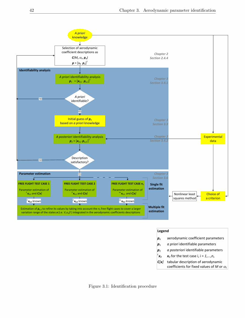
42 Chapter 3. Aerodynamic parameter identification
Parameter estimation
Selection of aerodynamic coefficient descriptions as
C(M, at, pa)
p = [x0 pa]T
Identifiability analysis
A posteriori identifiability analysis p2 = [x0,2 pa,2 ]
T
Description satisfactory?
FREE FLIGHT TEST CASE 1
Parameter estimation of 1 x0,2 and C[x]
FREE FLIGHT TEST CASE 2
Parameter estimation of 2 x0,2 and C[x]
FREE FLIGHT TEST CASE ns
Parameter estimation of ns x0,2 and C[x]
Estimation of pa,2 to refine its values by taking into account the ns free flight cases to cover a larger variation range of the states x (i.e. V,a,b ) integrated in the aerodynamic coefficients descriptions
1 x0,2 known 2 x0,2 known
Initial guess of pa
based on a priori knowledge
NO
YES
ns x0,2 known
Multiple fit estimation
Single fit estimation
A priori knowledge
Experimental data
Choice of a criterion
A priori identifiability analysisp1 = [x0,1 pa,1]T
YES
Nonlinear least squares method
Legend
pa
p1
p2 i x0
C[x]
A priori identifiable?
NO
aerodynamic coefficient parameters
a priori identifiable parameters
a posteriori identifiable parameters
x0 for the test case i, i = 1,...,ns
tabular description of aerodynamic coefficients for fixed values of M or at
Chapter 2Section 2.4.4
Chapter 3 Section 3.4.1
Chapter 3 Section 3.3
Chapter 3 Section 3.4.2
Chapter 3 Section 3.6
Figure 3.1: Identification procedure
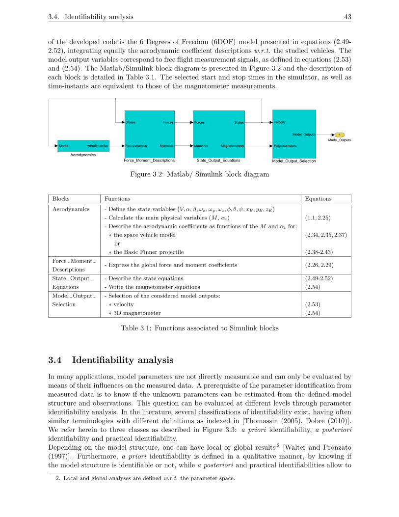
3.4. Identifiability analysis 43
of the developed code is the 6 Degrees of Freedom (6DOF) model presented in equations (2.49-2.52), integrating equally the aerodynamic coefficient descriptions w.r.t. the studied vehicles. Themodel output variables correspond to free flight measurement signals, as defined in equations (2.53)and (2.54). The Matlab/Simulink block diagram is presented in Figure 3.2 and the description ofeach block is detailed in Table 3.1. The selected start and stop times in the simulator, as well astime-instants are equivalent to those of the magnetometer measurements.
Model_Outputs
1
Model_Output_SelectionForce_Moment_Descriptions State_Output_EquationsAerodynamics
States Aerodynamics Aerodynamics
States Forces
Moments
Forces
Moments
States
Magnetometers Magnetometers
Velocity
Model_Outputs
Figure 3.2: Matlab/ Simulink block diagram
Blocks Functions Equations
Aerodynamics - Define the state variables (V, α, β, ωx, ωy, ωz, φ, θ, ψ, xE , yE , zE)- Calculate the main physical variables (M , αt) (1.1, 2.25)- Describe the aerodynamic coefficients as functions of the M and αt for:
∗ the space vehicle model (2.34, 2.35, 2.37)or
∗ the Basic Finner projectile (2.38-2.43)Force Moment - Express the global force and moment coefficients (2.26, 2.29)DescriptionsState Output - Describe the state equations (2.49-2.52)Equations - Write the magnetometer equations (2.54)Model Output - Selection of the considered model outputs:Selection ∗ velocity (2.53)
∗ 3D magnetometer (2.54)
Table 3.1: Functions associated to Simulink blocks
3.4 Identifiability analysis
In many applications, model parameters are not directly measurable and can only be evaluated bymeans of their influences on the measured data. A prerequisite of the parameter identification frommeasured data is to know if the unknown parameters can be estimated from the defined modelstructure and observations. This question can be evaluated at different levels through parameteridentifiability analysis. In the literature, several classifications of identifiability exist, having oftensimilar terminologies with different definitions as indexed in [Thomassin (2005), Dobre (2010)].We refer herein to three classes as described in Figure 3.3: a priori identifiability, a posterioriidentifiability and practical identifiability.Depending on the model structure, one can have local or global results 2 [Walter and Pronzato(1997)]. Furthermore, a priori identifiability is defined in a qualitative manner, by knowing ifthe model structure is identifiable or not, while a posteriori and practical identifiabilities allow to
2. Local and global analyses are defined w.r.t. the parameter space.
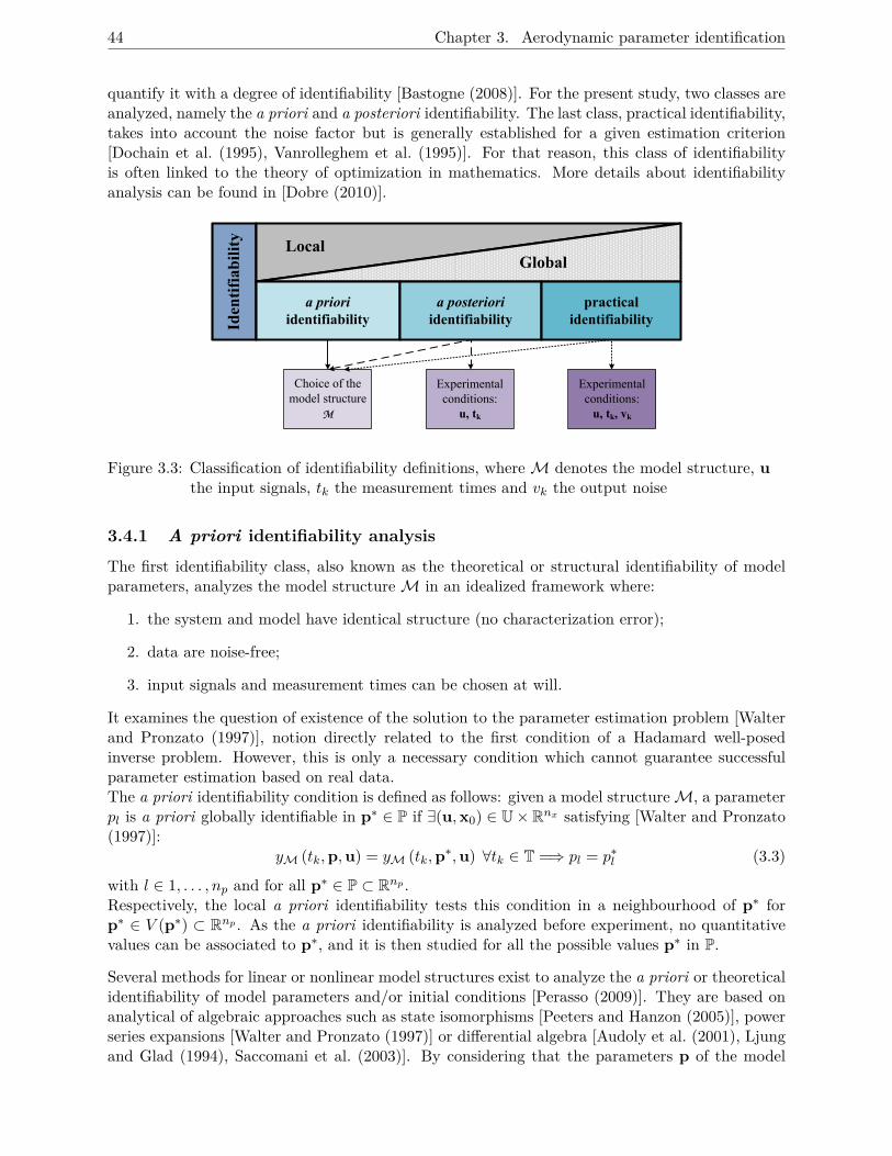
44 Chapter 3. Aerodynamic parameter identification
quantify it with a degree of identifiability [Bastogne (2008)]. For the present study, two classes areanalyzed, namely the a priori and a posteriori identifiability. The last class, practical identifiability,takes into account the noise factor but is generally established for a given estimation criterion[Dochain et al. (1995), Vanrolleghem et al. (1995)]. For that reason, this class of identifiabilityis often linked to the theory of optimization in mathematics. More details about identifiabilityanalysis can be found in [Dobre (2010)].
Identifiability
LocalGlobal
a priori
identifiabilitya posteriori
identifiabilitypractical
identifiability
Choice of themodel structure
M
Experimentalconditions:u, tk
Experimentalconditions:u, tk, vk
Figure 3.3: Classification of identifiability definitions, where M denotes the model structure, uthe input signals, tk the measurement times and vk the output noise
3.4.1 A priori identifiability analysis
The first identifiability class, also known as the theoretical or structural identifiability of modelparameters, analyzes the model structure M in an idealized framework where:
1. the system and model have identical structure (no characterization error);
2. data are noise-free;
3. input signals and measurement times can be chosen at will.
It examines the question of existence of the solution to the parameter estimation problem [Walterand Pronzato (1997)], notion directly related to the first condition of a Hadamard well-posedinverse problem. However, this is only a necessary condition which cannot guarantee successfulparameter estimation based on real data.The a priori identifiability condition is defined as follows: given a model structureM, a parameterpl is a priori globally identifiable in p∗ ∈ P if ∃(u,x0) ∈ U×Rnx satisfying [Walter and Pronzato(1997)]:
yM (tk,p,u) = yM (tk,p∗,u) ∀tk ∈ T =⇒ pl = p∗l (3.3)
with l ∈ 1, . . . , np and for all p∗ ∈ P ⊂ Rnp .Respectively, the local a priori identifiability tests this condition in a neighbourhood of p∗ forp∗ ∈ V (p∗) ⊂ Rnp . As the a priori identifiability is analyzed before experiment, no quantitativevalues can be associated to p∗, and it is then studied for all the possible values p∗ in P.
Several methods for linear or nonlinear model structures exist to analyze the a priori or theoreticalidentifiability of model parameters and/or initial conditions [Perasso (2009)]. They are based onanalytical of algebraic approaches such as state isomorphisms [Peeters and Hanzon (2005)], powerseries expansions [Walter and Pronzato (1997)] or differential algebra [Audoly et al. (2001), Ljungand Glad (1994), Saccomani et al. (2003)]. By considering that the parameters p of the model
3.4. Identifiability analysis 45
are a special kind of state variables satisfying p = 0, the local theoretical identifiability problem isdefined as a particular case of observability. In this sense, Sedoglavic has developed an algorithmfor testing local observability, relied on the differential algebra and it is based on the existence ofalgebraic relations between state variables and successive derivations of the inputs and the outputs[Sedoglavic (2002)]. It was implemented under the symbolic computation software MAPLE andreturns the number of non-identifiable parameters and that means that the remaining parametersp1 are locally theoretically identifiable. A description of this tool as well as an example of theobservability test is presented in Appendix C.
3.4.2 A posteriori identifiability analysis
The input design and experimental conditions are often subject to technical and/or economicalconstraints. In such restrictive experimental frameworks, even if a parameter is a priori identifiable,it may not be so in practice, due to a lack of information in the available observations. The existenceof the solution must then be verified from available data. The second class of identifiability, namelythe a posteriori identifiability is a particular case of the output distinguishability for a finitecollection of noise-free observations and given time instants, input signals and initial conditions,imposed by the experiments. The working assumptions are then defined as:
1. the system and model have identical structure (no characterization error);
2. data are noise-free;
3. input signals, initial conditions and measurement times are imposed by the experimentalconditions.
The a posteriori identifiability condition can be stated in a general manner as follows: givena model structure M with given input signals u and initial conditions x0, a parameter pl is aposteriori identifiable, if the following condition is satisfied [Walter and Pronzato (1997)]:
yM (tk,p,u) = yM (tk,p∗,u) ∀tk ∈ T =⇒ pl = p∗l (3.4)
with l ∈ 1, . . . , np and for almost all p∗ ∈ P ⊂ Rnp . In other words, the objective is to knowwhether this identical input-output behaviour implies that the parameters p of the model equalthose of the physical process p∗. For nonlinear models, this a posteriori identifiability condition isvalid only locally in a neighborhood V (p∗) of the true parameter values. The previous conditioncan also be expressed as
np∑l=1
∂y (tk,p,u)∂pl
∣∣∣∣p∗︸ ︷︷ ︸
sy/pl (tk,p∗,u)
·dpl = 0 =⇒ dp = 0 (3.5)
where sy/pl (tk,p∗,u) is the sensitivity function of the output variable y (tk,p∗,u) w.r.t. theparameter pl, for fixed input signals u and at a specific time instant tk. The difference is denotedby dp = p − p0, where p0 is the nominal value vector. As this application is characterized bythe absence of an input signal, for simplification reasons, the variables u will be omitted in thefollowing equations.The sensitivity analysis is an approach commonly used to assess the identifiability of the parametersfrom experimental conditions. It is employed in order to define if data contain enough informationto identify the parameters. As the sensitivity functions are defined by partial derivatives, dependent
46 Chapter 3. Aerodynamic parameter identification
of the time range or the nominal parameter values for example, sensitivity results will be localonly.
The parameters and output variables may have different measurement units and/or orders ofmagnitude. Generally, it is recommended to normalize the sensitivity functions sy/pl(tk,p
∗) w.r.t.the parameters, the outputs, or both variables. In the present study, it is normalized w.r.t. bothvariables defined as
sy/pl(tk,p∗) = sy/pl(tk,p
∗) · p∗l|y (tk,p∗) |1
(3.6)
with |.|1 the L1 norm.Taking into account the two previous equations, the parameters p2 are considered to be locally aposteriori identifiable if the empirical Fisher Information Matrix F is full rank, where F is definedas
F = Sy (p∗)T · Sy (p∗) (3.7)with Sy (p∗) ∈ RN×np the sensitivity matrix defined as
Sy (p∗) =
sy/p1 (t1,p∗) s
y/p2(t1,p∗) . . . sy/pnp (t1,p∗)
sy/p1 (t2,p∗) sy/p2 (t2,p∗) . . . sy/pnp (t2,p∗)...
... . . . ...sy/p1 (tN ,p∗) sy/p2 (tN ,p∗) . . . sy/pnp (tN ,p∗)
(3.8)
For multiple system outputs, the matrix F is computed based on a global sensitivity matrix Sygiven by
Sy =[
Sy1(p∗) Sy2(p∗) . . . Syny (p∗)]T (3.9)
where Syj (p∗) represents the normalised sensitivity matrix of the output variable yj , j = 1, · · · , ny,w.r.t. the parameters p∗ and ny corresponds to the number of output variables.However, if the rank of the empirical Fisher Information Matrix F is not full, one must select thea posteriori identifiable parameters. In that direction, several procedures exist in the literature[Weijers and Vanrolleghem (1997), Yao et al. (2003), Banks et al. (2013)] and are based on twoconditions that must be satisfied:
(C1) the output variables have to be sufficiently sensitive to individual changes in each parameterof p2;
(C2) the sensitivity functions must be linearly independent, as changes in the model output dueto a parameter variation may be compensated by appropriate changes in other parameters.
Several sensitivity measures allow to quantify the condition C1 [Brun et al. (2002), Li et al. (2004)],as for example:
δmsqrl =√
1N
sTy/pl sy/pl = 1√N· |sy/pl |2 (3.10)
δmabsl = 1N
N∑k=1|sy/pl(tk,p
∗)| = 1N· |sy/pl |1 (3.11)
δmeanl = 1N
N∑k=1
sy(tk, pl) (3.12)
δmaxl = maxk
sy(tk, pl) (3.13)
δminl = minksy(tk, pl) (3.14)
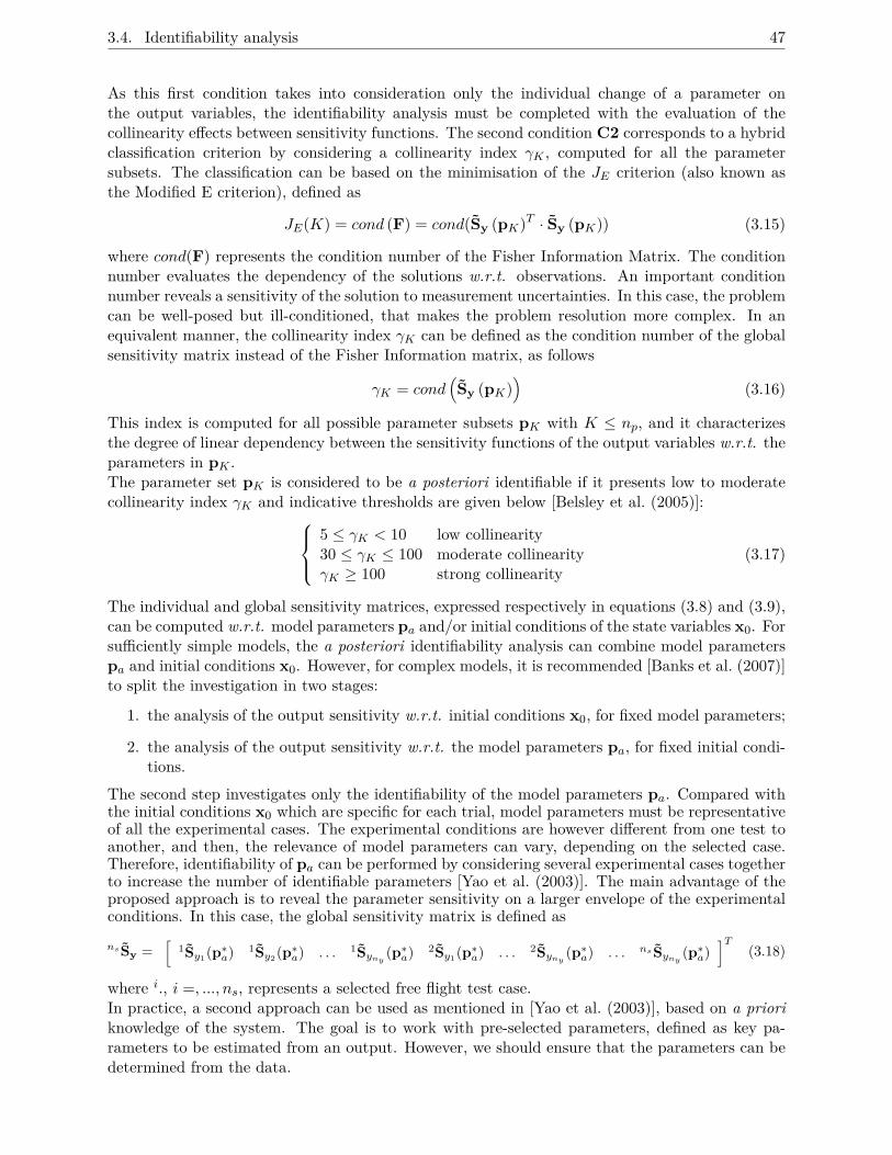
3.4. Identifiability analysis 47
As this first condition takes into consideration only the individual change of a parameter onthe output variables, the identifiability analysis must be completed with the evaluation of thecollinearity effects between sensitivity functions. The second condition C2 corresponds to a hybridclassification criterion by considering a collinearity index γK , computed for all the parametersubsets. The classification can be based on the minimisation of the JE criterion (also known asthe Modified E criterion), defined as
JE(K) = cond (F) = cond(Sy (pK)T · Sy (pK)) (3.15)
where cond(F) represents the condition number of the Fisher Information Matrix. The conditionnumber evaluates the dependency of the solutions w.r.t. observations. An important conditionnumber reveals a sensitivity of the solution to measurement uncertainties. In this case, the problemcan be well-posed but ill-conditioned, that makes the problem resolution more complex. In anequivalent manner, the collinearity index γK can be defined as the condition number of the globalsensitivity matrix instead of the Fisher Information matrix, as follows
γK = cond(Sy (pK)
)(3.16)
This index is computed for all possible parameter subsets pK with K ≤ np, and it characterizesthe degree of linear dependency between the sensitivity functions of the output variables w.r.t. theparameters in pK .The parameter set pK is considered to be a posteriori identifiable if it presents low to moderatecollinearity index γK and indicative thresholds are given below [Belsley et al. (2005)]:
5 ≤ γK < 10 low collinearity30 ≤ γK ≤ 100 moderate collinearityγK ≥ 100 strong collinearity
(3.17)
The individual and global sensitivity matrices, expressed respectively in equations (3.8) and (3.9),can be computed w.r.t. model parameters pa and/or initial conditions of the state variables x0. Forsufficiently simple models, the a posteriori identifiability analysis can combine model parameterspa and initial conditions x0. However, for complex models, it is recommended [Banks et al. (2007)]to split the investigation in two stages:
1. the analysis of the output sensitivity w.r.t. initial conditions x0, for fixed model parameters;
2. the analysis of the output sensitivity w.r.t. the model parameters pa, for fixed initial condi-tions.
The second step investigates only the identifiability of the model parameters pa. Compared withthe initial conditions x0 which are specific for each trial, model parameters must be representativeof all the experimental cases. The experimental conditions are however different from one test toanother, and then, the relevance of model parameters can vary, depending on the selected case.Therefore, identifiability of pa can be performed by considering several experimental cases togetherto increase the number of identifiable parameters [Yao et al. (2003)]. The main advantage of theproposed approach is to reveal the parameter sensitivity on a larger envelope of the experimentalconditions. In this case, the global sensitivity matrix is defined as
ns Sy =[
1Sy1(p∗a) 1Sy2(p∗
a) . . . 1Syny(p∗a) 2Sy1(p∗
a) . . . 2Syny(p∗a) . . . ns Syny
(p∗a)]T
(3.18)
where i., i =, ..., ns, represents a selected free flight test case.In practice, a second approach can be used as mentioned in [Yao et al. (2003)], based on a prioriknowledge of the system. The goal is to work with pre-selected parameters, defined as key pa-rameters to be estimated from an output. However, we should ensure that the parameters can bedetermined from the data.
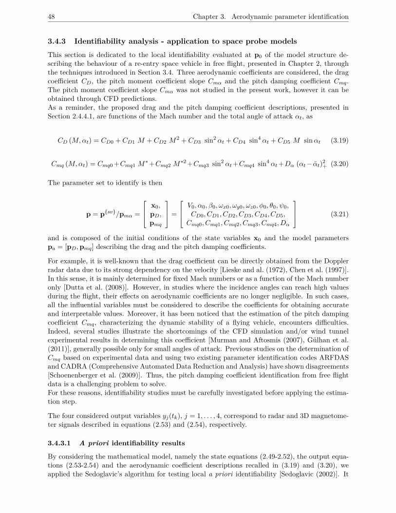
48 Chapter 3. Aerodynamic parameter identification
3.4.3 Identifiability analysis - application to space probe models
This section is dedicated to the local identifiability evaluated at p0 of the model structure de-scribing the behaviour of a re-entry space vehicle in free flight, presented in Chapter 2, throughthe techniques introduced in Section 3.4. Three aerodynamic coefficients are considered, the dragcoefficient CD, the pitch moment coefficient slope Cmα and the pitch damping coefficient Cmq.The pitch moment coefficient slope Cmα was not studied in the present work, however it can beobtained through CFD predictions.As a reminder, the proposed drag and the pitch damping coefficient descriptions, presented inSection 2.4.4.1, are functions of the Mach number and the total angle of attack αt, as
CD (M,αt) = CD0 + CD1 M + CD2 M2 + CD3 sin2 αt + CD4 sin4 αt + CD5 M sinαt (3.19)
Cmq (M,αt) = Cmq0 +Cmq1 M∗+Cmq2 M
∗2 +Cmq3 sin2 αt+Cmq4 sin4 αt+Dα (αt− αt)2+ (3.20)
The parameter set to identify is then
p = p{sv}/pmα =
x0,pD,pmq
=
V0, α0, β0, ωx0, ωy0, ωz0, φ0, θ0, ψ0,CD0, CD1, CD2, CD3, CD4, CD5,Cmq0, Cmq1, Cmq2, Cmq3, Cmq4, Dα
(3.21)
and is composed of the initial conditions of the state variables x0 and the model parameterspa = [pD,pmq] describing the drag and the pitch damping coefficients.
For example, it is well-known that the drag coefficient can be directly obtained from the Dopplerradar data due to its strong dependency on the velocity [Lieske and al. (1972), Chen et al. (1997)].In this sense, it is mainly determined for fixed Mach numbers or as a function of the Mach numberonly [Dutta et al. (2008)]. However, in studies where the incidence angles can reach high valuesduring the flight, their effects on aerodynamic coefficients are no longer negligible. In such cases,all the influential variables must be considered to describe the coefficients for obtaining accurateand interpretable values. Moreover, it has been noticed that the estimation of the pitch dampingcoefficient Cmq, characterizing the dynamic stability of a flying vehicle, encounters difficulties.Indeed, several studies illustrate the shortcomings of the CFD simulation and/or wind tunnelexperimental results in determining this coefficient [Murman and Aftosmis (2007), Gulhan et al.(2011)], generally possible only for small angles of attack. Previous studies on the determination ofCmq based on experimental data and using two existing parameter identification codes ARFDASand CADRA (Comprehensive Automated Data Reduction and Analysis) have shown disagreements[Schoenenberger et al. (2009)]. Thus, the pitch damping coefficient identification from free flightdata is a challenging problem to solve.For these reasons, identifiability studies must be carefully investigated before applying the estima-tion step.
The four considered output variables yj(tk), j = 1, . . . , 4, correspond to radar and 3D magnetome-ter signals described in equations (2.53) and (2.54), respectively.
3.4.3.1 A priori identifiability results
By considering the mathematical model, namely the state equations (2.49-2.52), the output equa-tions (2.53-2.54) and the aerodynamic coefficient descriptions recalled in (3.19) and (3.20), weapplied the Sedoglavic’s algorithm for testing local a priori identifiability [Sedoglavic (2002)]. It
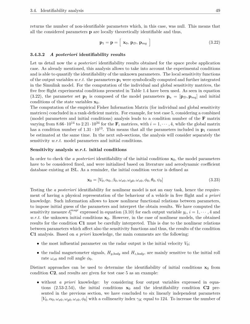
3.4. Identifiability analysis 49
returns the number of non-identifiable parameters which, in this case, was null. This means thatall the considered parameters p are locally theoretically identifiable and thus,
p1 = p =[
x0, pD, pmq]
(3.22)
3.4.3.2 A posteriori identifiability results
Let us detail now the a posteriori identifiability results obtained for the space probe applicationcase. As already mentioned, this analysis allows to take into account the experimental conditionsand is able to quantify the identifiability of the unknown parameters. The local sensitivity functionsof the output variables w.r.t. the parameters p1 were symbolically computed and further integratedin the Simulink model. For the computation of the individual and global sensitivity matrices, thefive free flight experimental conditions presented in Table 1.4 have been used. As seen in equation(3.22), the parameter set p1 is composed of the model parameters pa = [pD,pmq] and initialconditions of the state variables x0.The computation of the empirical Fisher Information Matrix (for individual and global sensitivitymatrices) concluded in a rank-deficient matrix. For example, for test case 5, considering a combined(model parameters and initial conditions) analysis leads to a condition number of the F matrixvarying from 8.66 ·1014 to 2.21 ·1034 for the Fi matrices, with i = 1, · · · , 4, while the global matrixhas a condition number of 1.31 · 1013. This means that all the parameters included in p1 cannotbe estimated at the same time. In the next sub-sections, the analysis will consider separately thesensitivity w.r.t. model parameters and initial conditions.
Sensitivity analysis w.r.t. initial conditions
In order to check the a posteriori identifiability of the initial conditions x0, the model parametershave to be considered fixed, and were initialized based on literature and aerodynamic coefficientdatabase existing at ISL. As a reminder, the initial condition vector is defined as
x0 = [V0, α0, β0, ωx0, ωy0, ωz0, φ0, θ0, ψ0] (3.23)
Testing the a posteriori identifiability for nonlinear model is not an easy task, hence the require-ment of having a physical representation of the behaviour of a vehicle in free flight and a prioriknowledge. Such information allows to know nonlinear functional relations between parameters,to impose initial guess of the parameters and interpret the obtain results. We have computed thesensitivity measure δmsqrl expressed in equation (3.10) for each output variable yi, i = 1, · · · , 4 andw.r.t. the unknown initial conditions x0. However, in the case of nonlinear models, the obtainedresults for the condition C1 must be carefully interpreted. This is due to the nonlinear relationsbetween parameters which affect also the sensitivity functions and thus, the results of the conditionC1 analysis. Based on a priori knowledge, the main comments are the following:
• the most influential parameter on the radar output is the initial velocity V0;
• the radial magnetometer signals, Hy,body and Hz,body, are mainly sensitive to the initial rollrate ωx0 and roll angle φ0.
Distinct approaches can be used to determine the identifiability of initial conditions x0 fromcondition C2, and results are given for test case 5 as an example:
• without a priori knowledge: by considering four output variables expressed in equa-tions (2.53-2.54), the initial conditions x0 and the identifiability condition C2 pre-sented in the previous section, we have concluded to six linearly independent parameters[V0, α0, ωx0, ωy0, ωz0, φ0] with a collinearity index γK equal to 124. To increase the number of
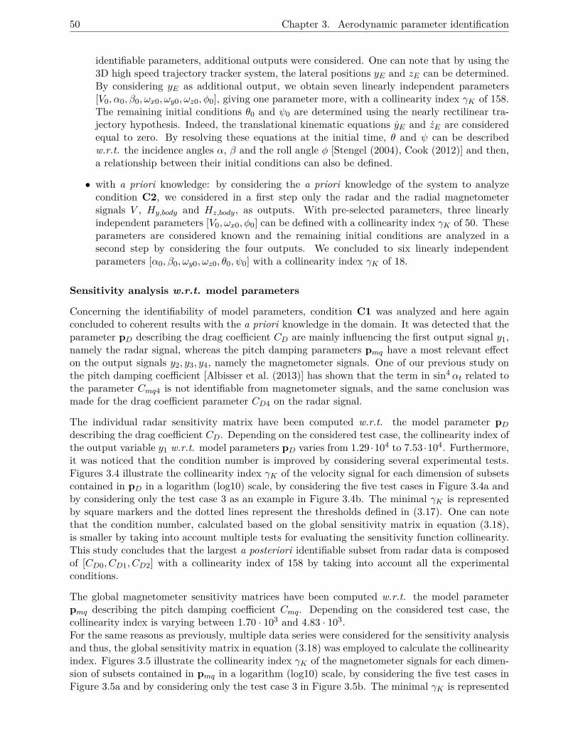
50 Chapter 3. Aerodynamic parameter identification
identifiable parameters, additional outputs were considered. One can note that by using the3D high speed trajectory tracker system, the lateral positions yE and zE can be determined.By considering yE as additional output, we obtain seven linearly independent parameters[V0, α0, β0, ωx0, ωy0, ωz0, φ0], giving one parameter more, with a collinearity index γK of 158.The remaining initial conditions θ0 and ψ0 are determined using the nearly rectilinear tra-jectory hypothesis. Indeed, the translational kinematic equations yE and zE are consideredequal to zero. By resolving these equations at the initial time, θ and ψ can be describedw.r.t. the incidence angles α, β and the roll angle φ [Stengel (2004), Cook (2012)] and then,a relationship between their initial conditions can also be defined.
• with a priori knowledge: by considering the a priori knowledge of the system to analyzecondition C2, we considered in a first step only the radar and the radial magnetometersignals V , Hy,body and Hz,body, as outputs. With pre-selected parameters, three linearlyindependent parameters [V0, ωx0, φ0] can be defined with a collinearity index γK of 50. Theseparameters are considered known and the remaining initial conditions are analyzed in asecond step by considering the four outputs. We concluded to six linearly independentparameters [α0, β0, ωy0, ωz0, θ0, ψ0] with a collinearity index γK of 18.
Sensitivity analysis w.r.t. model parameters
Concerning the identifiability of model parameters, condition C1 was analyzed and here againconcluded to coherent results with the a priori knowledge in the domain. It was detected that theparameter pD describing the drag coefficient CD are mainly influencing the first output signal y1,namely the radar signal, whereas the pitch damping parameters pmq have a most relevant effecton the output signals y2, y3, y4, namely the magnetometer signals. One of our previous study onthe pitch damping coefficient [Albisser et al. (2013)] has shown that the term in sin4 αt related tothe parameter Cmq4 is not identifiable from magnetometer signals, and the same conclusion wasmade for the drag coefficient parameter CD4 on the radar signal.
The individual radar sensitivity matrix have been computed w.r.t. the model parameter pDdescribing the drag coefficient CD. Depending on the considered test case, the collinearity index ofthe output variable y1 w.r.t. model parameters pD varies from 1.29 ·104 to 7.53 ·104. Furthermore,it was noticed that the condition number is improved by considering several experimental tests.Figures 3.4 illustrate the collinearity index γK of the velocity signal for each dimension of subsetscontained in pD in a logarithm (log10) scale, by considering the five test cases in Figure 3.4a andby considering only the test case 3 as an example in Figure 3.4b. The minimal γK is representedby square markers and the dotted lines represent the thresholds defined in (3.17). One can notethat the condition number, calculated based on the global sensitivity matrix in equation (3.18),is smaller by taking into account multiple tests for evaluating the sensitivity function collinearity.This study concludes that the largest a posteriori identifiable subset from radar data is composedof [CD0, CD1, CD2] with a collinearity index of 158 by taking into account all the experimentalconditions.
The global magnetometer sensitivity matrices have been computed w.r.t. the model parameterpmq describing the pitch damping coefficient Cmq. Depending on the considered test case, thecollinearity index is varying between 1.70 · 103 and 4.83 · 103.For the same reasons as previously, multiple data series were considered for the sensitivity analysisand thus, the global sensitivity matrix in equation (3.18) was employed to calculate the collinearityindex. Figures 3.5 illustrate the collinearity index γK of the magnetometer signals for each dimen-sion of subsets contained in pmq in a logarithm (log10) scale, by considering the five test cases inFigure 3.5a and by considering only the test case 3 in Figure 3.5b. The minimal γK is represented
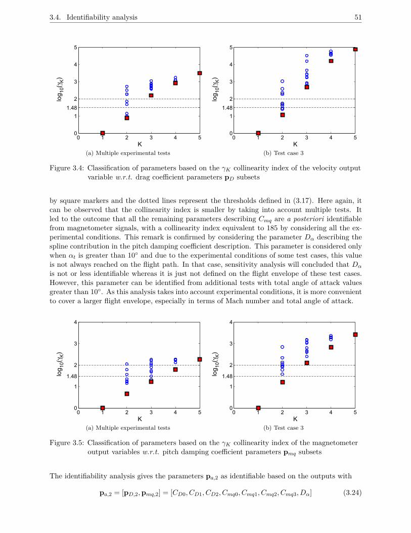
3.4. Identifiability analysis 51
0 1 2 3 4 50
1
1.48
2
3
4
5
K
log10(γK)
(a) Multiple experimental tests
0 1 2 3 4 50
1
1.48
2
3
4
5
K
log10(γK)
(b) Test case 3
Figure 3.4: Classification of parameters based on the γK collinearity index of the velocity outputvariable w.r.t. drag coefficient parameters pD subsets
by square markers and the dotted lines represent the thresholds defined in (3.17). Here again, itcan be observed that the collinearity index is smaller by taking into account multiple tests. Itled to the outcome that all the remaining parameters describing Cmq are a posteriori identifiablefrom magnetometer signals, with a collinearity index equivalent to 185 by considering all the ex-perimental conditions. This remark is confirmed by considering the parameter Dα describing thespline contribution in the pitch damping coefficient description. This parameter is considered onlywhen αt is greater than 10◦ and due to the experimental conditions of some test cases, this valueis not always reached on the flight path. In that case, sensitivity analysis will concluded that Dα
is not or less identifiable whereas it is just not defined on the flight envelope of these test cases.However, this parameter can be identified from additional tests with total angle of attack valuesgreater than 10◦. As this analysis takes into account experimental conditions, it is more convenientto cover a larger flight envelope, especially in terms of Mach number and total angle of attack.
0 1 2 3 4 50
1
1.48
2
3
4
K
log10(γK)
(a) Multiple experimental tests
0 1 2 3 4 50
1
1.48
2
3
4
K
log10(γK)
(b) Test case 3
Figure 3.5: Classification of parameters based on the γK collinearity index of the magnetometeroutput variables w.r.t. pitch damping coefficient parameters pmq subsets
The identifiability analysis gives the parameters pa,2 as identifiable based on the outputs with
pa,2 = [pD,2,pmq,2] = [CD0, CD1, CD2, Cmq0, Cmq1, Cmq2, Cmq3, Dα] (3.24)
52 Chapter 3. Aerodynamic parameter identification
Therefore, identifiability analysis leads to the following main conclusions:
• the a priori identifiability analysis showed that all the parameters can be considered aslocally identifiable. This implies that the model structure is well posed in the Hadamardsense;
• as the empirical Fisher Information Matrix was found to be rank deficient, two classificationcriteria were further used in order to select the a posteriori identifiable parameters and theinitial conditions x0 and the model parameters were analyzed separately;
• with the integration of a priori knowledge, we obtain sensitivity functions w.r.t. x0 whichare linearly independent and thus, all the initial conditions can be identified;
• all the model parameters, except the parameters CD4 and Cmq4, are sufficiently sensitive toinfluence at least one output variable and eight of them can be considered as being linearlyindependent;
• the sensitivity matrix computed based on multiple data series showed a better conditionnumber and therefore improves the identifiability of the parameters;
• the identifiability results are coherent with a priori knowledge in the domain.
3.5 Estimation of aerodynamic parameters
This section details the employed strategy for the aerodynamic parameter estimation. A 6DOFcode already exists at ISL for the aerodynamic coefficient determination but presents severallimitations, especially concerning the aerodynamic coefficient representations. They are describedin a tabular form, for fixed values of Mach numbers or total angles of attack αt. For this reasonand in order to improve the accuracy and the understanding of the estimated coefficients, a newinverse 6DOF code included several improvements was developed.
The parameter estimation is achieved through the use of the developed code, denoted as Inv6DoF,implemented under Matlab/ Simulink. The model implementation was presented in Section 3.3 anda Matlab code was developed and integrated into the tool to proceed to the aerodynamic parameterestimation from a single and/or a multiple fit strategy. The parameters are estimated by usinga traditional iterative nonlinear Least Squares method. The a posteriori identifiability is meantto guide the estimation process. The identifiability analyses proposed to check the identifiabilityof the initial conditions x0 and the model parameters pa in two stages. For the same reasons, anestimation procedure composed of two distinct steps and illustrated in Figure 3.1 was applied:
1. the first step, defined as a single fit estimation strategy, aims at determining the initial con-ditions x0,2 and the aerodynamic coefficients C[x] for each data series i, with i = 1, · · · , ns.This step is considered as an intermediate phase to mainly determine the initial conditionsof each trial. To obtain preliminary aerodynamic values, the coefficients C[x] are estimatedin a tabular form, for fixed Mach number or total angle of attack values.
2. the second step is dedicated to the estimation of the aerodynamic coefficients, described aspolynomial functions dependent of the state variables and model parameters pa, based onseveral data series. To increase the probability that the coefficients define the vehicle’s aero-dynamics over the entire range of test conditions and to improve the accuracy of the estimatedcoefficients, a multiple fit strategy was considered. As all the free flight tests are conductedwith the same vehicle, this strategy attempts to obtain meaningful aerodynamic coefficientsevolution as a function of the Mach number and the total angle of attack which should be
3.6. Concluding remarks 53
valid for all test cases. Moreover, it allows to cover a larger envelope of variation of bothvariables and provides a common set of aerodynamic coefficients that are determined frommultiple data series simultaneously analyzed, that gives a more complete spectrum of thevehicle’s motion. As identifiability analysis based on a combination of data sets improves thenumber of identifiable parameters, this strategy will also improve the parameter estimation.The combination of multiple data series was already used to provide a better representa-tion of the flight envelope and improve the estimated aerodynamic coefficients [Dupuis andHathaway (1997)] but only in a tabular form for constant Mach numbers. Several techniqueswere presented in the literature [Leith et al. (1993)] by using superposition, concatenation ormultiple cost approaches. The last one is the most adapted to the case of nonlinear systemsand allows to preserve all the information revealed through single fit identification.The multiple cost function approach was applied and the estimation criterion for the secondstep is then defined as follows:
J(pa,2) =ns∑i=1
Ji(pa,2) (3.25)
where pa,2 are the a posteriori identifiable parameters describing aerodynamic coefficients.
3.6 Concluding remarks
In this chapter, the proposed grey-box model identification procedure for the aerodynamic pa-rameter estimation has been presented. It is composed of six main steps, from the definition ofthe model structure to the parameter estimation issue. The intermediate steps are the modelimplementation and the identifiability analysis. The implemented model represents the kernelof the inverse 6DOF code developed in the frame of this study. As the structure of the modelis nonlinear, the identifiability results are only local. Nevertheless, if the identifiability resultsare carefully interpreted, they allow to guide the estimation process. They brought to light thecomplexity of the analysis when initial conditions and model parameters are considered and whennonlinear dependency between parameters is observed. It was also shown that using multiple datasets for the sensitivity analysis allowed to increase the number of identifiable parameters. In thissense, the same strategy was used for the parametric estimation of the aerodynamic coefficients.The multiple fit strategy presents many advantages as covering a larger flight envelope, in termsof Mach numbers and total angles of attack, and obtaining meaningful aerodynamic coefficientsvalid for several test cases.Even if the identifiability analyses were performed only for the space probe case, similar conclusionscan be made for the projectile concerning the initial conditions. For the projectile aerodynamiccoefficients, simplified descriptions were used due to the limited number of trials to validate poly-nomial descriptions. This is more widely explained in the next chapter dedicated to the applicationresults for space probe and projectile cases.

54 Chapter 3. Aerodynamic parameter identification
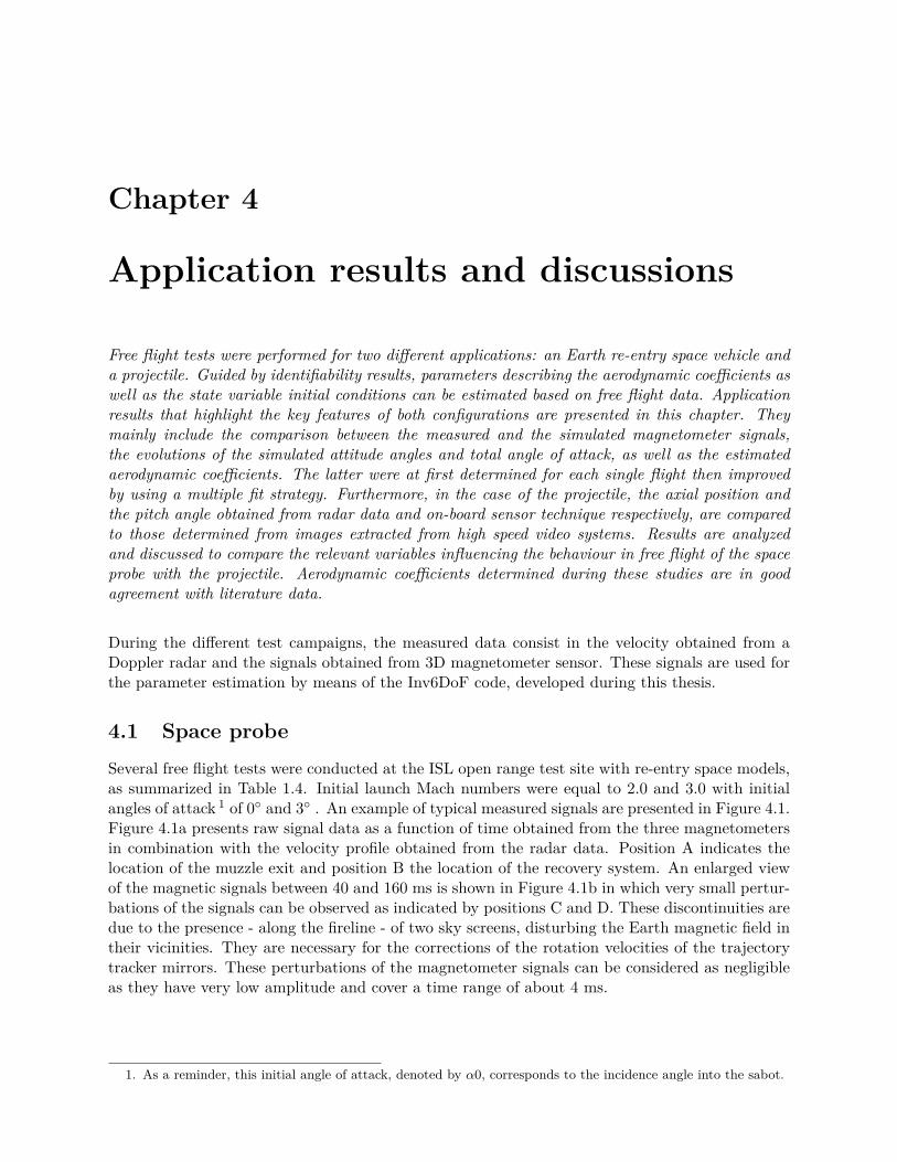
Chapter 4
Application results and discussions
Free flight tests were performed for two different applications: an Earth re-entry space vehicle anda projectile. Guided by identifiability results, parameters describing the aerodynamic coefficients aswell as the state variable initial conditions can be estimated based on free flight data. Applicationresults that highlight the key features of both configurations are presented in this chapter. Theymainly include the comparison between the measured and the simulated magnetometer signals,the evolutions of the simulated attitude angles and total angle of attack, as well as the estimatedaerodynamic coefficients. The latter were at first determined for each single flight then improvedby using a multiple fit strategy. Furthermore, in the case of the projectile, the axial position andthe pitch angle obtained from radar data and on-board sensor technique respectively, are comparedto those determined from images extracted from high speed video systems. Results are analyzedand discussed to compare the relevant variables influencing the behaviour in free flight of the spaceprobe with the projectile. Aerodynamic coefficients determined during these studies are in goodagreement with literature data.
During the different test campaigns, the measured data consist in the velocity obtained from aDoppler radar and the signals obtained from 3D magnetometer sensor. These signals are used forthe parameter estimation by means of the Inv6DoF code, developed during this thesis.
4.1 Space probe
Several free flight tests were conducted at the ISL open range test site with re-entry space models,as summarized in Table 1.4. Initial launch Mach numbers were equal to 2.0 and 3.0 with initialangles of attack 1 of 0◦ and 3◦ . An example of typical measured signals are presented in Figure 4.1.Figure 4.1a presents raw signal data as a function of time obtained from the three magnetometersin combination with the velocity profile obtained from the radar data. Position A indicates thelocation of the muzzle exit and position B the location of the recovery system. An enlarged viewof the magnetic signals between 40 and 160 ms is shown in Figure 4.1b in which very small pertur-bations of the signals can be observed as indicated by positions C and D. These discontinuities aredue to the presence - along the fireline - of two sky screens, disturbing the Earth magnetic field intheir vicinities. They are necessary for the corrections of the rotation velocities of the trajectorytracker mirrors. These perturbations of the magnetometer signals can be considered as negligibleas they have very low amplitude and cover a time range of about 4 ms.
1. As a reminder, this initial angle of attack, denoted by α0, corresponds to the incidence angle into the sabot.
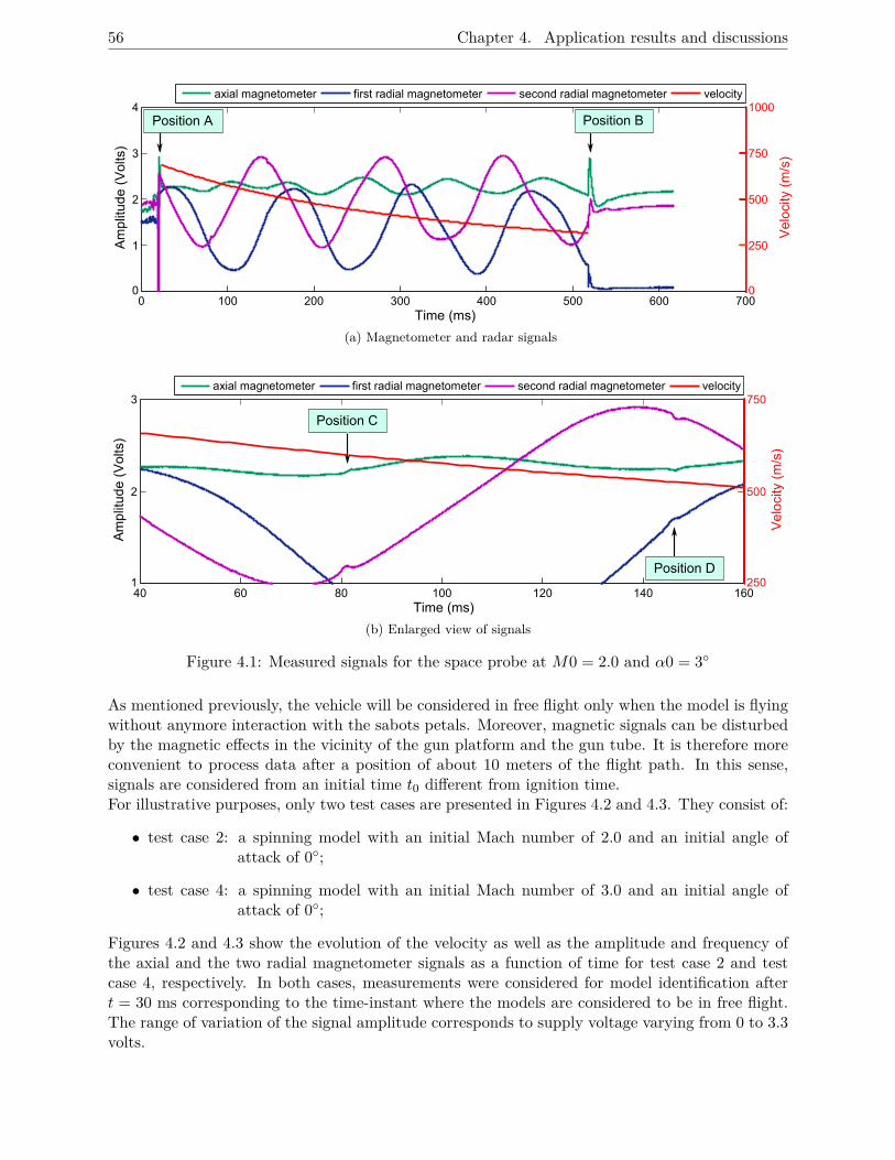
56 Chapter 4. Application results and discussions
0 100 200 300 400 500 600 7000
1
2
3
4
Timer(ms)
Am
plit
ude
r(V
olts
)
0
250
500
750
1000
Ve
loci
tyr(
m/s
)
axial magnetometer first radial magnetometer second radial magnetometer velocity
PositionrA PositionrB
(a) Magnetometer and radar signals
40 60 80 100 120 140 1601
2
3
Timen(ms)
Am
plit
ude
n(V
olts
)
250
500
750
Ve
loci
tyn(
m/s
)
axial magnetometer first radial magnetometer second radial magnetometer velocity
PositionnC
PositionnD
(b) Enlarged view of signals
Figure 4.1: Measured signals for the space probe at M0 = 2.0 and α0 = 3◦
As mentioned previously, the vehicle will be considered in free flight only when the model is flyingwithout anymore interaction with the sabots petals. Moreover, magnetic signals can be disturbedby the magnetic effects in the vicinity of the gun platform and the gun tube. It is therefore moreconvenient to process data after a position of about 10 meters of the flight path. In this sense,signals are considered from an initial time t0 different from ignition time.For illustrative purposes, only two test cases are presented in Figures 4.2 and 4.3. They consist of:
• test case 2: a spinning model with an initial Mach number of 2.0 and an initial angle ofattack of 0◦;
• test case 4: a spinning model with an initial Mach number of 3.0 and an initial angle ofattack of 0◦;
Figures 4.2 and 4.3 show the evolution of the velocity as well as the amplitude and frequency ofthe axial and the two radial magnetometer signals as a function of time for test case 2 and testcase 4, respectively. In both cases, measurements were considered for model identification aftert = 30 ms corresponding to the time-instant where the models are considered to be in free flight.The range of variation of the signal amplitude corresponds to supply voltage varying from 0 to 3.3volts.
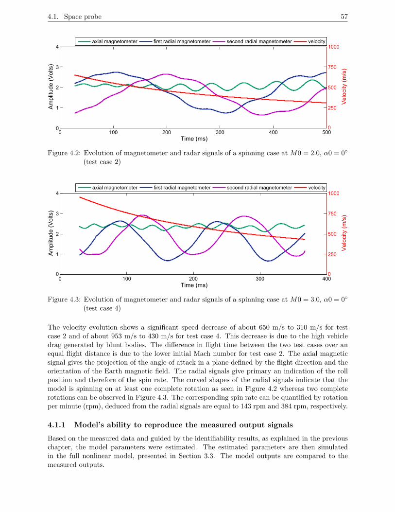
4.1. Space probe 57
0 100 200 300 400 5000
1
2
3
4
Time (ms)
Amplitude(Volts)
0
250
500
750
1000
Velocity(m/s)
axial magnetometer first radial magnetometer second radial magnetometer velocity
Figure 4.2: Evolution of magnetometer and radar signals of a spinning case at M0 = 2.0, α0 = 0◦(test case 2)
0 100 200 300 4000
1
2
3
4
Time (ms)
Amplitude(Volts)
0
250
500
750
1000
Velocity(m/s)
axial magnetometer first radial magnetometer second radial magnetometer velocity
Figure 4.3: Evolution of magnetometer and radar signals of a spinning case at M0 = 3.0, α0 = 0◦(test case 4)
The velocity evolution shows a significant speed decrease of about 650 m/s to 310 m/s for testcase 2 and of about 953 m/s to 430 m/s for test case 4. This decrease is due to the high vehicledrag generated by blunt bodies. The difference in flight time between the two test cases over anequal flight distance is due to the lower initial Mach number for test case 2. The axial magneticsignal gives the projection of the angle of attack in a plane defined by the flight direction and theorientation of the Earth magnetic field. The radial signals give primary an indication of the rollposition and therefore of the spin rate. The curved shapes of the radial signals indicate that themodel is spinning on at least one complete rotation as seen in Figure 4.2 whereas two completerotations can be observed in Figure 4.3. The corresponding spin rate can be quantified by rotationper minute (rpm), deduced from the radial signals are equal to 143 rpm and 384 rpm, respectively.
4.1.1 Model’s ability to reproduce the measured output signals
Based on the measured data and guided by the identifiability results, as explained in the previouschapter, the model parameters were estimated. The estimated parameters are then simulatedin the full nonlinear model, presented in Section 3.3. The model outputs are compared to themeasured outputs.
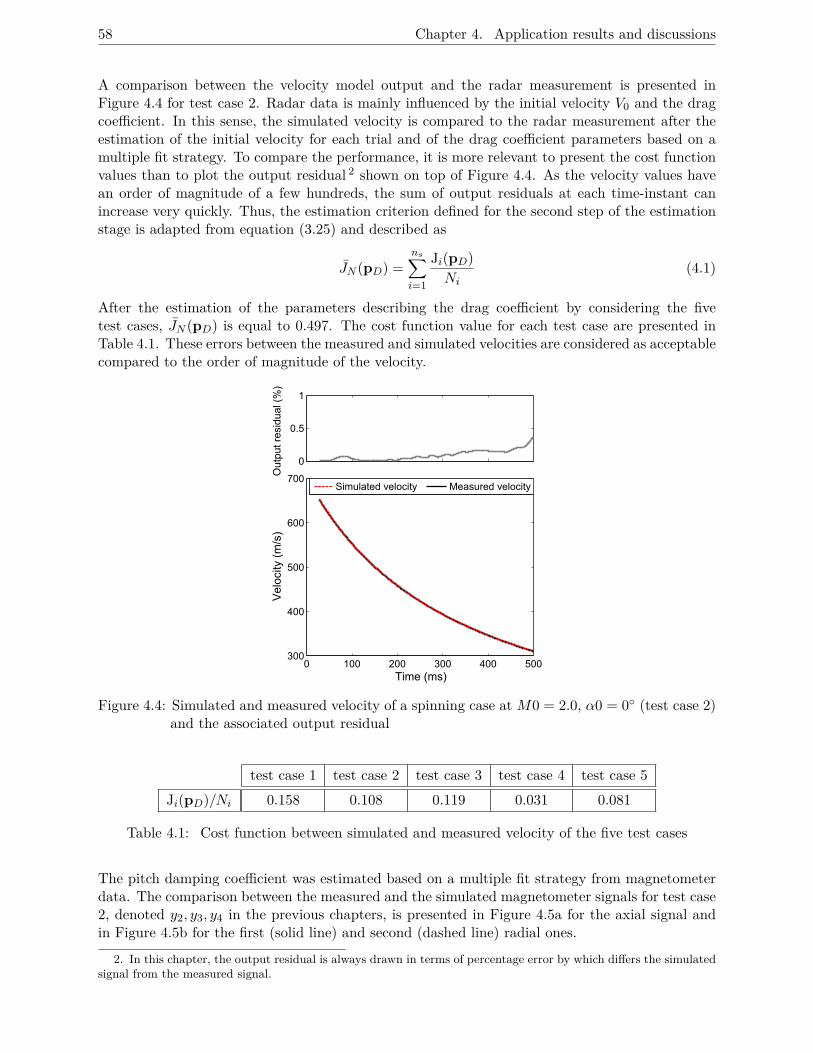
58 Chapter 4. Application results and discussions
A comparison between the velocity model output and the radar measurement is presented inFigure 4.4 for test case 2. Radar data is mainly influenced by the initial velocity V0 and the dragcoefficient. In this sense, the simulated velocity is compared to the radar measurement after theestimation of the initial velocity for each trial and of the drag coefficient parameters based on amultiple fit strategy. To compare the performance, it is more relevant to present the cost functionvalues than to plot the output residual 2 shown on top of Figure 4.4. As the velocity values havean order of magnitude of a few hundreds, the sum of output residuals at each time-instant canincrease very quickly. Thus, the estimation criterion defined for the second step of the estimationstage is adapted from equation (3.25) and described as
JN (pD) =ns∑i=1
Ji(pD)Ni
(4.1)
After the estimation of the parameters describing the drag coefficient by considering the fivetest cases, JN (pD) is equal to 0.497. The cost function value for each test case are presented inTable 4.1. These errors between the measured and simulated velocities are considered as acceptablecompared to the order of magnitude of the velocity.
0
0.5
1
0 100 200 300 400 500300
400
500
600
700
TimeO(ms)
Vel
ocity
O(m
/s)
Measured velocitySimulated velocity
Out
putOr
esid
ualO(
%)
Figure 4.4: Simulated and measured velocity of a spinning case at M0 = 2.0, α0 = 0◦ (test case 2)and the associated output residual
test case 1 test case 2 test case 3 test case 4 test case 5Ji(pD)/Ni 0.158 0.108 0.119 0.031 0.081
Table 4.1: Cost function between simulated and measured velocity of the five test cases
The pitch damping coefficient was estimated based on a multiple fit strategy from magnetometerdata. The comparison between the measured and the simulated magnetometer signals for test case2, denoted y2, y3, y4 in the previous chapters, is presented in Figure 4.5a for the axial signal andin Figure 4.5b for the first (solid line) and second (dashed line) radial ones.
2. In this chapter, the output residual is always drawn in terms of percentage error by which differs the simulatedsignal from the measured signal.
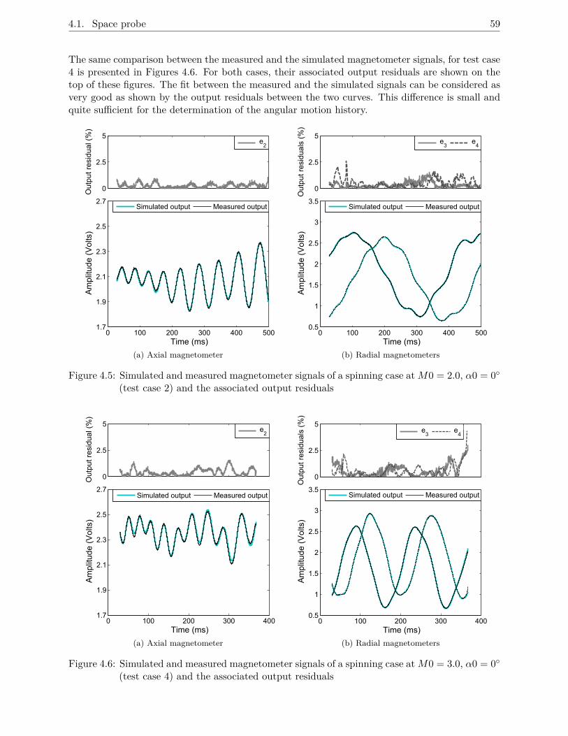
4.1. Space probe 59
The same comparison between the measured and the simulated magnetometer signals, for test case4 is presented in Figures 4.6. For both cases, their associated output residuals are shown on thetop of these figures. The fit between the measured and the simulated signals can be considered asvery good as shown by the output residuals between the two curves. This difference is small andquite sufficient for the determination of the angular motion history.
0
2.5
5e
2
0 100 200 300 400 5001.7
1.9
2.1
2.3
2.5
2.7
Time (ms)
Am
plit
ude
(Vol
ts)
Simulated output Measured output
Out
put r
esid
ual (
%)
(a) Axial magnetometer
0
2.5
5e
3e
4
0 100 200 300 400 5000.5
1
1.5
2
2.5
3
3.5
Time (ms)
Am
plit
ude
(Vol
ts)
Simulated output Measured output
Out
put r
esid
uals
(%
)
(b) Radial magnetometers
Figure 4.5: Simulated and measured magnetometer signals of a spinning case at M0 = 2.0, α0 = 0◦(test case 2) and the associated output residuals
0
2.5
5e
2
0 100 200 300 4001.7
1.9
2.1
2.3
2.5
2.7
Time (ms)
Am
plit
ude
(Vol
ts)
Simulated output Measured output
Out
put r
esid
ual (
%)
(a) Axial magnetometer
0
2.5
5e
3e
4
0 100 200 300 4000.5
1
1.5
2
2.5
3
3.5
Time (ms)
Am
plit
ude
(Vol
ts)
Simulated output Measured output
Out
put r
esid
uals
(%
)
(b) Radial magnetometers
Figure 4.6: Simulated and measured magnetometer signals of a spinning case at M0 = 3.0, α0 = 0◦(test case 4) and the associated output residuals
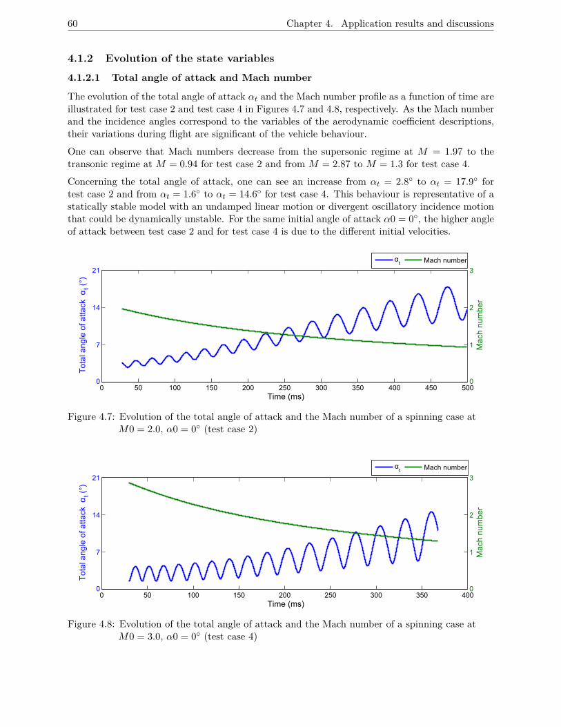
60 Chapter 4. Application results and discussions
4.1.2 Evolution of the state variables
4.1.2.1 Total angle of attack and Mach number
The evolution of the total angle of attack αt and the Mach number profile as a function of time areillustrated for test case 2 and test case 4 in Figures 4.7 and 4.8, respectively. As the Mach numberand the incidence angles correspond to the variables of the aerodynamic coefficient descriptions,their variations during flight are significant of the vehicle behaviour.
One can observe that Mach numbers decrease from the supersonic regime at M = 1.97 to thetransonic regime at M = 0.94 for test case 2 and from M = 2.87 to M = 1.3 for test case 4.
Concerning the total angle of attack, one can see an increase from αt = 2.8◦ to αt = 17.9◦ fortest case 2 and from αt = 1.6◦ to αt = 14.6◦ for test case 4. This behaviour is representative of astatically stable model with an undamped linear motion or divergent oscillatory incidence motionthat could be dynamically unstable. For the same initial angle of attack α0 = 0◦, the higher angleof attack between test case 2 and for test case 4 is due to the different initial velocities.
0 50 100 150 200 250 300 350 400 450 5000
7
14
21
Time (ms)
To
tal a
ng
le o
f atta
ckα
t(°
)
0
1
2
3
Ma
ch n
um
be
r
αt Mach number
Figure 4.7: Evolution of the total angle of attack and the Mach number of a spinning case atM0 = 2.0, α0 = 0◦ (test case 2)
0 50 100 150 200 250 300 350 4000
7
14
21
Time (ms)
To
tal a
ng
le o
f atta
ckα
t(°
)
0
1
2
3M
ach
nu
mb
er
αt Mach number
Figure 4.8: Evolution of the total angle of attack and the Mach number of a spinning case atM0 = 3.0, α0 = 0◦ (test case 4)
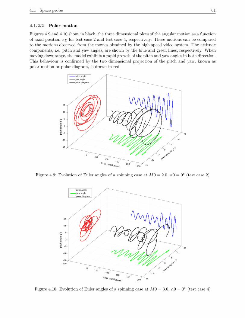
4.1. Space probe 61
4.1.2.2 Polar motion
Figures 4.9 and 4.10 show, in black, the three dimensional plots of the angular motion as a functionof axial position xE for test case 2 and test case 4, respectively. These motions can be comparedto the motions observed from the movies obtained by the high speed video system. The attitudecomponents, i.e. pitch and yaw angles, are shown by the blue and green lines, respectively. Whenmoving downrange, the model exhibits a rapid growth of the pitch and yaw angles in both direction.This behaviour is confirmed by the two dimensional projection of the pitch and yaw, known aspolar motion or polar diagram, is drawn in red.
-21
-14
-7
0
7
14
21
050
100150
200250
-21
-14
-7
0
7
14
21
yaw a
ngle (°
)
axial position (m)
pitc
h a
ng
le (
°)
pitch angle
yaw angle
polar diagram
Figure 4.9: Evolution of Euler angles of a spinning case at M0 = 2.0, α0 = 0◦ (test case 2)
yaw a
ngle (°
)
-21
-14
-7
0
7
14
21
-100
050
100150
200250
-21
-14
-7
0
7
14
21
axial position (m)
pitc
h a
ng
le (
°)
pitch angle
yaw angle
polar diagram
Figure 4.10: Evolution of Euler angles of a spinning case at M0 = 3.0, α0 = 0◦ (test case 4)
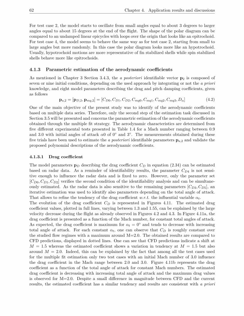
62 Chapter 4. Application results and discussions
For test case 2, the model starts to oscillate from small angles equal to about 3 degrees to largerangles equal to about 15 degrees at the end of the flight. The shape of the polar diagram can becompared to an undamped linear epicycles with loops over the origin that looks like an epitrochoid.For test case 4, the model seems to behave the same way as for test case 2, starting from small tolarge angles but more randomly. In this case the polar diagram looks more like an hypotrochoid.Usually, hypotrochoid motions are more representative of fin stabilized shells while spin stabilizedshells behave more like epitrochoids.
4.1.3 Parametric estimation of the aerodynamic coefficients
As mentioned in Chapter 3 Section 3.4.3, the a posteriori identifiable vector p2 is composed ofseven or nine initial conditions, depending on the used approach by integrating or not the a prioriknowledge, and eight model parameters describing the drag and pitch damping coefficients, givenas follows
pa,2 = [pD,2,pmq,2] = [CD0, CD1, CD2, Cmq0, Cmq1, Cmq2, Cmq3, Dα] (4.2)
One of the main objective of the present study was to identify of the aerodynamic coefficientsbased on multiple data series. Therefore, only the second step of the estimation task discussed inSection 3.5 will be presented and concerns the parametric estimation of the aerodynamic coefficientsobtained through the multiple fit strategy. The aerodynamic characteristics are determined fromfive different experimental tests presented in Table 1.4 for a Mach number ranging between 0.9and 3.0 with initial angles of attack α0 of 0◦ and 3◦. The measurements obtained during thesefive trials have been used to estimate the a posteriori identifiable parameters pa,2 and validate theproposed polynomial descriptions of the aerodynamic coefficients.
4.1.3.1 Drag coefficient
The model parameters pD describing the drag coefficient CD in equation (2.34) can be estimatedbased on radar data. As a reminder of identifiability results, the parameter CD4 is not sensi-tive enough to influence the radar data and is fixed to zero. However, only the parameter set[CD0, CD1, CD2] verifies the second condition of the identifiability analysis and can be simultane-ously estimated. As the radar data is also sensitive to the remaining parameters [CD3, CD5], aniterative estimation was used to identify also parameters depending on the total angle of attack.That allows to refine the tendency of the drag coefficient w.r.t. the influential variable αt.The evolution of the drag coefficient CD is represented in Figures 4.11. The estimated dragcoefficient values, plotted in full lines, varying between 1.3 and 1.55, can be explained by the largevelocity decrease during the flight as already observed in Figures 4.2 and 4.3. In Figure 4.11a, thedrag coefficient is presented as a function of the Mach number, for constant total angles of attack.As expected, the drag coefficient is maximum for αt = 0◦ and tends to decrease with increasingtotal angle of attack. For each constant αt, one can observe that CD is roughly constant overthe studied flow regimes with a maximum around M=2.0. The obtained results are compared toCFD predictions, displayed in dotted lines. One can see that CFD predictions indicate a shift atM = 1.5 whereas the estimated coefficient shows a variation in tendency at M = 1.5 but alsoaround M = 2.0. Indeed, this can be explained by the fact that among all the test cases usedfor the multiple fit estimation only two test cases with an initial Mach number of 3.0 influencethe drag coefficient in the Mach range between 2.0 and 3.0. Figure 4.11b represents the dragcoefficient as a function of the total angle of attack for constant Mach numbers. The estimateddrag coefficient is decreasing with increasing total angle of attack and the maximum drag valuesis observed for M=2.0. Despite a small difference in magnitude between CFD and the currentresults, the estimated coefficient has a similar tendency and results are consistent with a priori
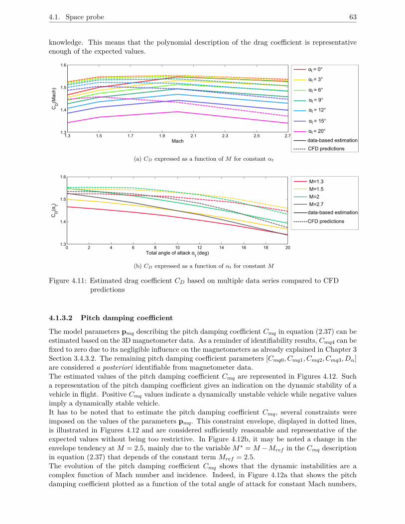
4.1. Space probe 63
knowledge. This means that the polynomial description of the drag coefficient is representativeenough of the expected values.
1.3 1.5 1.7 1.9 2.1 2.3 2.5 2.71.3
1.4
1.5
1.6
Mach
CD
(Ma
ch)
αtF=F0°
αtF=F3°
αtF=F6°
αtF=F9°
αtF=F12°
data-basedFestimation
CFDFpredictions
αtF=F15°
αtF=F20°
(a) CD expressed as a function of M for constant αt
0 2 4 6 8 10 12 14 16 18 201.3
1.4
1.5
1.6
Totalsanglesofsattack αt(deg)
CD
(αt)
M=1.3
M=1.5
M=2
M=2.7
data-basedsestimation
CFDspredictions
(b) CD expressed as a function of αt for constant M
Figure 4.11: Estimated drag coefficient CD based on multiple data series compared to CFDpredictions
4.1.3.2 Pitch damping coefficient
The model parameters pmq describing the pitch damping coefficient Cmq in equation (2.37) can beestimated based on the 3D magnetometer data. As a reminder of identifiability results, Cmq4 can befixed to zero due to its negligible influence on the magnetometers as already explained in Chapter 3Section 3.4.3.2. The remaining pitch damping coefficient parameters [Cmq0, Cmq1, Cmq2, Cmq3, Dα]are considered a posteriori identifiable from magnetometer data.The estimated values of the pitch damping coefficient Cmq are represented in Figures 4.12. Sucha representation of the pitch damping coefficient gives an indication on the dynamic stability of avehicle in flight. Positive Cmq values indicate a dynamically unstable vehicle while negative valuesimply a dynamically stable vehicle.It has to be noted that to estimate the pitch damping coefficient Cmq, several constraints wereimposed on the values of the parameters pmq. This constraint envelope, displayed in dotted lines,is illustrated in Figures 4.12 and are considered sufficiently reasonable and representative of theexpected values without being too restrictive. In Figure 4.12b, it may be noted a change in theenvelope tendency at M = 2.5, mainly due to the variable M∗ = M −Mref in the Cmq descriptionin equation (2.37) that depends of the constant term Mref = 2.5.The evolution of the pitch damping coefficient Cmq shows that the dynamic instabilities are acomplex function of Mach number and incidence. Indeed, in Figure 4.12a that shows the pitchdamping coefficient plotted as a function of the total angle of attack for constant Mach numbers,
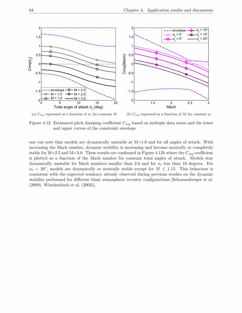
64 Chapter 4. Application results and discussions
0 5 10 15 20-2
-1.5
-1
-0.5
0
0.5
1
1.5
2
Total angle of attack αt(deg)
Cmq(αt)
M = 1.0M = 2.0M = 2.5M = 3.0
envelope
M = 1.5
(a) Cmq expressed as a function of αt for constant M
1 1.5 2 2.5 3-2
-1.5
-1
-0.5
0
0.5
1
1.5
2
Mach
Cmq(Mach)
αt= 0°
αt= 5°
αt= 10°
αt= 15°
αt= 20°
envelope
(b) Cmq expressed as a function of M for constant αt
Figure 4.12: Estimated pitch damping coefficient Cmq based on multiple data series and the lowerand upper curves of the constraint envelope
one can note that models are dynamically unstable at M=1.0 and for all angles of attack. Withincreasing the Mach number, dynamic stability is increasing and become neutrally or completelystable for M=2.5 and M=3.0. These results are confirmed in Figure 4.12b where the Cmq coefficientis plotted as a function of the Mach number for constant total angles of attack. Models staydynamically unstable for Mach numbers smaller than 2.0 and for αt less than 10 degrees. Forαt = 20◦, models are dynamically or neutrally stable except for M ≤ 1.15. This behaviour isconsistent with the expected tendency already observed during previous studies on the dynamicstability performed for different blunt atmospheric re-entry configurations [Schoenenberger et al.(2009), Winchenbach et al. (2002)].
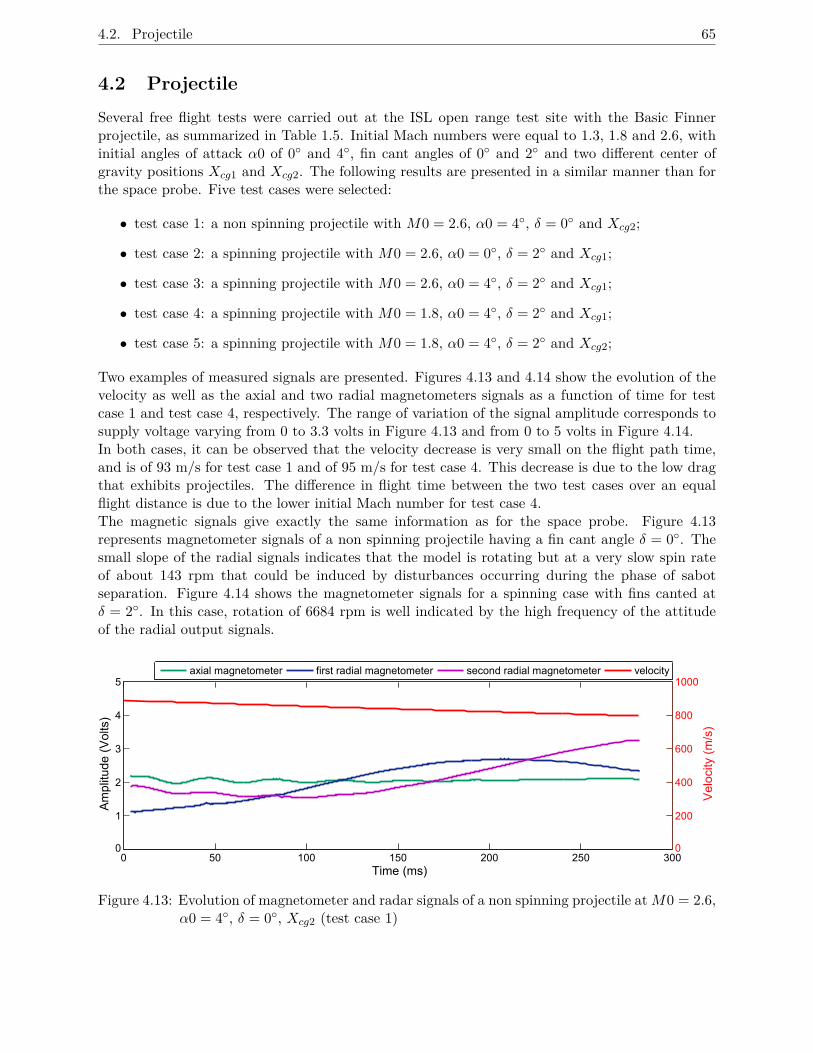
4.2. Projectile 65
4.2 Projectile
Several free flight tests were carried out at the ISL open range test site with the Basic Finnerprojectile, as summarized in Table 1.5. Initial Mach numbers were equal to 1.3, 1.8 and 2.6, withinitial angles of attack α0 of 0◦ and 4◦, fin cant angles of 0◦ and 2◦ and two different center ofgravity positions Xcg1 and Xcg2. The following results are presented in a similar manner than forthe space probe. Five test cases were selected:
• test case 1: a non spinning projectile with M0 = 2.6, α0 = 4◦, δ = 0◦ and Xcg2;
• test case 2: a spinning projectile with M0 = 2.6, α0 = 0◦, δ = 2◦ and Xcg1;
• test case 3: a spinning projectile with M0 = 2.6, α0 = 4◦, δ = 2◦ and Xcg1;
• test case 4: a spinning projectile with M0 = 1.8, α0 = 4◦, δ = 2◦ and Xcg1;
• test case 5: a spinning projectile with M0 = 1.8, α0 = 4◦, δ = 2◦ and Xcg2;
Two examples of measured signals are presented. Figures 4.13 and 4.14 show the evolution of thevelocity as well as the axial and two radial magnetometers signals as a function of time for testcase 1 and test case 4, respectively. The range of variation of the signal amplitude corresponds tosupply voltage varying from 0 to 3.3 volts in Figure 4.13 and from 0 to 5 volts in Figure 4.14.In both cases, it can be observed that the velocity decrease is very small on the flight path time,and is of 93 m/s for test case 1 and of 95 m/s for test case 4. This decrease is due to the low dragthat exhibits projectiles. The difference in flight time between the two test cases over an equalflight distance is due to the lower initial Mach number for test case 4.The magnetic signals give exactly the same information as for the space probe. Figure 4.13represents magnetometer signals of a non spinning projectile having a fin cant angle δ = 0◦. Thesmall slope of the radial signals indicates that the model is rotating but at a very slow spin rateof about 143 rpm that could be induced by disturbances occurring during the phase of sabotseparation. Figure 4.14 shows the magnetometer signals for a spinning case with fins canted atδ = 2◦. In this case, rotation of 6684 rpm is well indicated by the high frequency of the attitudeof the radial output signals.
0 50 100 150 200 250 3000
1
2
3
4
5
Time (ms)
Amplitude(Volts)
0
200
400
600
800
1000
Velocity(m/s)
axial magnetometer first radial magnetometer second radial magnetometer velocity
Figure 4.13: Evolution of magnetometer and radar signals of a non spinning projectile at M0 = 2.6,α0 = 4◦, δ = 0◦, Xcg2 (test case 1)
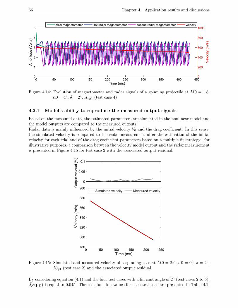
66 Chapter 4. Application results and discussions
0 50 100 150 200 250 300 350 400 4500
1
2
3
4
5
Time (ms)
Amplitude(Volts)
0
200
400
600
800
1000
Velocity(m/s)
axial magnetometer first radial magnetometer second radial magnetometer velocity
Figure 4.14: Evolution of magnetometer and radar signals of a spinning projectile at M0 = 1.8,α0 = 4◦, δ = 2◦, Xcg1 (test case 4)
4.2.1 Model’s ability to reproduce the measured output signals
Based on the measured data, the estimated parameters are simulated in the nonlinear model andthe model outputs are compared to the measured outputs.Radar data is mainly influenced by the initial velocity V0 and the drag coefficient. In this sense,the simulated velocity is compared to the radar measurement after the estimation of the initialvelocity for each trial and of the drag coefficient parameters based on a multiple fit strategy. Forillustrative purposes, a comparison between the velocity model output and the radar measurementis presented in Figure 4.15 for test case 2 with the associated output residual.
0
0.05
0.1
0 50 100 150 200 250780
800
820
840
860
880
900
TimeS(ms)
Vel
ocity
S(m
/s)
Measured velocitySimulated velocity
Out
putSr
esid
ualS(
%)
Figure 4.15: Simulated and measured velocity of a spinning case at M0 = 2.6, α0 = 0◦, δ = 2◦,Xcg1 (test case 2) and the associated output residual
By considering equation (4.1) and the four test cases with a fin cant angle of 2◦ (test cases 2 to 5),JN (pD) is equal to 0.045. The cost function values for each test case are presented in Table 4.2.
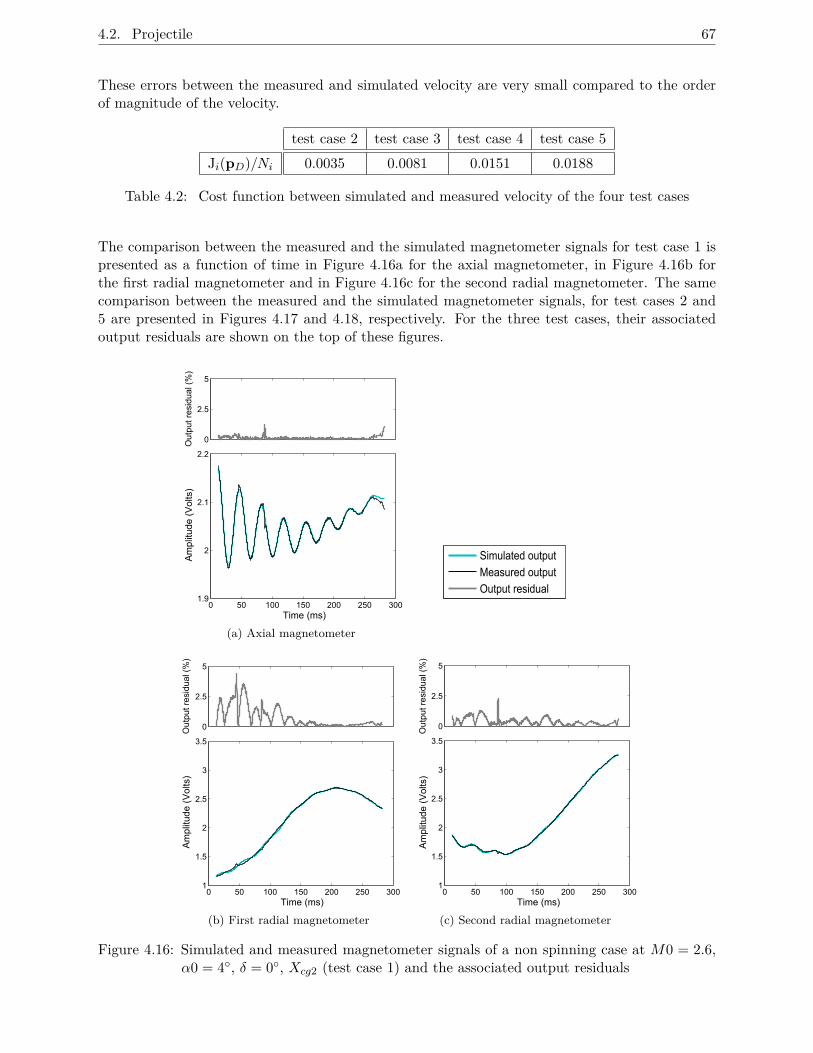
4.2. Projectile 67
These errors between the measured and simulated velocity are very small compared to the orderof magnitude of the velocity.
test case 2 test case 3 test case 4 test case 5Ji(pD)/Ni 0.0035 0.0081 0.0151 0.0188
Table 4.2: Cost function between simulated and measured velocity of the four test cases
The comparison between the measured and the simulated magnetometer signals for test case 1 ispresented as a function of time in Figure 4.16a for the axial magnetometer, in Figure 4.16b forthe first radial magnetometer and in Figure 4.16c for the second radial magnetometer. The samecomparison between the measured and the simulated magnetometer signals, for test cases 2 and5 are presented in Figures 4.17 and 4.18, respectively. For the three test cases, their associatedoutput residuals are shown on the top of these figures.
0
2.5
5
0 50 100 150 200 250 3001.9
2
2.1
2.2
Time (ms)
Am
plit
ude
(V
olts
)O
utpu
t res
idua
l (%
)
(a) Axial magnetometer
Simulated output
Measured output
Output residual
0
2.5
5
0 50 100 150 200 250 3001
1.5
2
2.5
3
3.5
Time (ms)
Am
plit
ude
(V
olts
)O
utpu
t res
idua
l (%
)
(b) First radial magnetometer
0
2.5
5
0 50 100 150 200 250 3001
1.5
2
2.5
3
3.5
Time (ms)
Am
plit
ude
(V
olts
)O
utpu
t res
idua
l (%
)
(c) Second radial magnetometer
Figure 4.16: Simulated and measured magnetometer signals of a non spinning case at M0 = 2.6,α0 = 4◦, δ = 0◦, Xcg2 (test case 1) and the associated output residuals
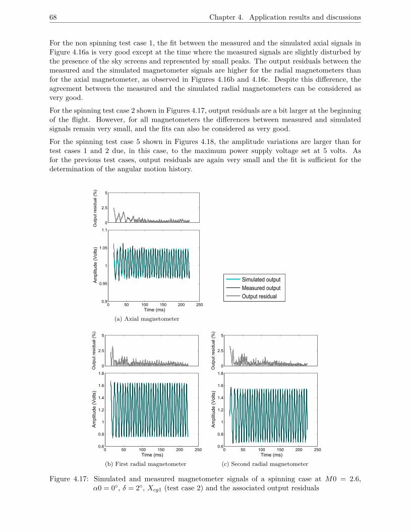
68 Chapter 4. Application results and discussions
For the non spinning test case 1, the fit between the measured and the simulated axial signals inFigure 4.16a is very good except at the time where the measured signals are slightly disturbed bythe presence of the sky screens and represented by small peaks. The output residuals between themeasured and the simulated magnetometer signals are higher for the radial magnetometers thanfor the axial magnetometer, as observed in Figures 4.16b and 4.16c. Despite this difference, theagreement between the measured and the simulated radial magnetometers can be considered asvery good.
For the spinning test case 2 shown in Figures 4.17, output residuals are a bit larger at the beginningof the flight. However, for all magnetometers the differences between measured and simulatedsignals remain very small, and the fits can also be considered as very good.
For the spinning test case 5 shown in Figures 4.18, the amplitude variations are larger than fortest cases 1 and 2 due, in this case, to the maximum power supply voltage set at 5 volts. Asfor the previous test cases, output residuals are again very small and the fit is sufficient for thedetermination of the angular motion history.
0
2.5
5
Out
put r
esid
ual (
%)
0 50 100 150 200 2500.9
0.95
1
1.05
1.1
Time (ms)
Am
plit
ude
(V
olts
)
(a) Axial magnetometer
Simulated output
Measured output
Output residual
0
2.5
5
0 50 100 150 200 2500.6
0.8
1
1.2
1.4
1.6
1.8
Time (ms)
Am
plit
ude
(V
olts
)O
utpu
t res
idua
l (%
)
(b) First radial magnetometer
0
2.5
5
0 50 100 150 200 2500.6
0.8
1
1.2
1.4
1.6
1.8
Time (ms)
Am
plit
ude
(V
olts
)O
utpu
t res
idua
l (%
)
(c) Second radial magnetometer
Figure 4.17: Simulated and measured magnetometer signals of a spinning case at M0 = 2.6,α0 = 0◦, δ = 2◦, Xcg1 (test case 2) and the associated output residuals
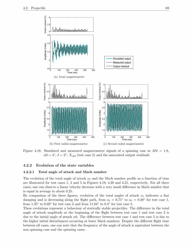
4.2. Projectile 69
0
2.5
5
0 100 200 300 400 5002.8
3
3.2
3.4
3.6
Time (ms)
Am
plit
ude
(V
olts
)O
utpu
t res
idua
l (%
)
(a) Axial magnetometer
Simulated output
Measured output
Output residual
0
2.5
5
0 100 200 300 400 5001
1.5
2
2.5
3
3.5
4
Time (ms)
Am
plit
ude
(V
olts
)O
utpu
t res
idua
l (%
)
(b) First radial magnetometer
0
2.5
5
0 100 200 300 400 5001
1.5
2
2.5
3
3.5
4
Time (ms)
Am
plit
ude
(V
olts
)O
utpu
t res
idua
l (%
)
(c) Second radial magnetometer
Figure 4.18: Simulated and measured magnetometer signals of a spinning case at M0 = 1.8,α0 = 4◦, δ = 2◦, Xcg2 (test case 5) and the associated output residuals
4.2.2 Evolution of the state variables
4.2.2.1 Total angle of attack and Mach number
The evolution of the total angle of attack αt and the Mach number profile as a function of timeare illustrated for test cases 1, 2 and 5 in Figures 4.19, 4.20 and 4.21, respectively. For all threecases, one can observe a linear velocity decrease with a very small difference in Mach number thatis equal in average to about 0.25.By comparison of the three figures, evolution of the total angles of attack αt indicates a fastdamping and is decreasing along the flight path, from αt = 6.71◦ to αt = 0.38◦ for test case 1,from 1.35◦ to 0.03◦ for test case 2 and from 11.04◦ to 0.4◦ for test case 5.These evolutions represent a behaviour of statically stable projectiles. The difference in the totalangle of attack amplitude at the beginning of the flight between test case 1 and test case 2 isdue to the initial angle of attack α0. The difference between test case 1 and test case 5 is due tothe higher initial disturbances occurring at lower Mach numbers. Despite the different flight timebetween all cases, one can note that the frequency of the angle of attack is equivalent between thenon spinning case and the spinning cases.
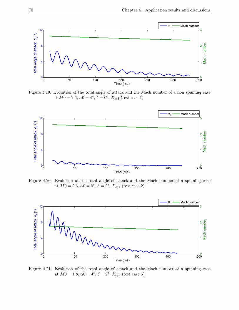
70 Chapter 4. Application results and discussions
0 50 100 150 200 250 3000
4
8
12
Time (ms)
To
tal a
ng
le o
f atta
ckα
t(°
)
0
1
2
3
Ma
ch n
um
be
r
αt Mach number
Figure 4.19: Evolution of the total angle of attack and the Mach number of a non spinning caseat M0 = 2.6, α0 = 4◦, δ = 0◦, Xcg2 (test case 1)
0 50 100 150 200 2500
4
8
12
Time (ms)
To
tal a
ng
le o
f atta
ckα
t(°
)
0
1
2
3
Ma
ch n
um
be
r
αt Mach number
Figure 4.20: Evolution of the total angle of attack and the Mach number of a spinning caseat M0 = 2.6, α0 = 0◦, δ = 2◦, Xcg1 (test case 2)
0 100 200 300 400 5000
4
8
12
Time (ms)
To
tal a
ng
le o
f atta
ckα
t(°
)
0
1
2
3M
ach
nu
mb
er
αt Mach number
Figure 4.21: Evolution of the total angle of attack and the Mach number of a spinning caseat M0 = 1.8, α0 = 4◦, δ = 2◦, Xcg2 (test case 5)
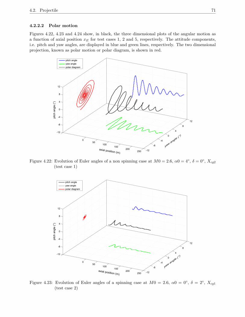
4.2. Projectile 71
4.2.2.2 Polar motion
Figures 4.22, 4.23 and 4.24 show, in black, the three dimensional plots of the angular motion asa function of axial position xE for test cases 1, 2 and 5, respectively. The attitude components,i.e. pitch and yaw angles, are displayed in blue and green lines, respectively. The two dimensionalprojection, known as polar motion or polar diagram, is shown in red.
-12
-8
-4
0
4
8
12
050
100150
200250
-12
-8
-4
0
4
8
12
pitc
h a
ng
le (
°)
yaw a
ngle (°)
axial position (m)
pitch angle
yaw angle
polar diagram
Figure 4.22: Evolution of Euler angles of a non spinning case at M0 = 2.6, α0 = 4◦, δ = 0◦, Xcg2(test case 1)
-12
-8
-4
0
4
8
12
050
100150
200250
-12
-8
-4
0
4
8
12
yaw a
ngle (°)
axial position (m)
pitc
h a
ng
le (
°)
pitch angle
yaw angle
polar diagram
Figure 4.23: Evolution of Euler angles of a spinning case at M0 = 2.6, α0 = 0◦, δ = 2◦, Xcg1(test case 2)
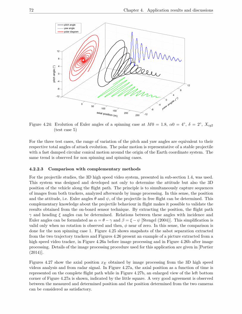
72 Chapter 4. Application results and discussions
-12
-8
-4
0
4
8
12
050
100150
200250
-12
-8
-4
0
4
8
12
pitch angle
yaw angle
polar diagram
yaw a
ngle (°)
axial position (m)
pitc
h a
ng
le (
°)
Figure 4.24: Evolution of Euler angles of a spinning case at M0 = 1.8, α0 = 4◦, δ = 2◦, Xcg2(test case 5)
For the three test cases, the range of variation of the pitch and yaw angles are equivalent to theirrespective total angles of attack evolution. The polar motion is representative of a stable projectilewith a fast damped circular conical motion around the origin of the Earth coordinate system. Thesame trend is observed for non spinning and spinning cases.
4.2.2.3 Comparison with complementary methods
For the projectile studies, the 3D high speed video system, presented in sub-section 1.4, was used.This system was designed and developed not only to determine the attitude but also the 3Dposition of the vehicle along the flight path. The principle is to simultaneously capture sequencesof images from both trackers, analyzed afterwards by image processing. In this sense, the positionand the attitude, i.e. Euler angles θ and ψ, of the projectile in free flight can be determined. Thiscomplementary knowledge about the projectile behaviour in flight makes it possible to validate theresults obtained from the on-board sensor technique. By extracting the position, the flight pathγ and heading ξ angles can be determined. Relations between these angles with incidence andEuler angles can be formulated as α = θ− γ and β = ξ−ψ [Stengel (2004)]. This simplification isvalid only when no rotation is observed and then, φ near of zero. In this sense, the comparison isdone for the non spinning case 1. Figure 4.25 shows snapshots of the sabot separation extractedfrom the two trajectory trackers and Figures 4.26 present an example of a picture extracted from ahigh speed video tracker, in Figure 4.26a before image processing and in Figure 4.26b after imageprocessing. Details of the image processing procedure used for this application are given in [Portier(2014)].
Figures 4.27 show the axial position xE obtained by image processing from the 3D high speedvideos analysis and from radar signal. In Figure 4.27a, the axial position as a function of time isrepresented on the complete flight path while in Figure 4.27b, an enlarged view of the left bottomcorner of Figure 4.27a is shown, indicated by the little square. A very good agreement is observedbetween the measured and determined position and the position determined from the two camerascan be considered as satisfactory.
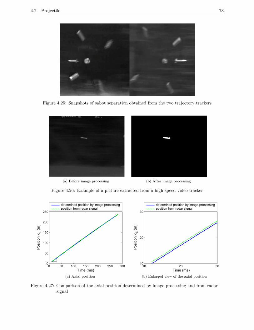
4.2. Projectile 73
Figure 4.25: Snapshots of sabot separation obtained from the two trajectory trackers
(a) Before image processing (b) After image processing
Figure 4.26: Example of a picture extracted from a high speed video tracker
0 50 100 150 200 250 3000
50
100
150
200
250
Time (ms)
Po
sitio
n x E
(m)
determined position by image processingposition from radar signal
(a) Axial position
10 20 3010
20
30
Time (ms)
Po
sitio
n x E
(m)
determined position by image processingposition from radar signal
(b) Enlarged view of the axial position
Figure 4.27: Comparison of the axial position determined by image processing and from radarsignal
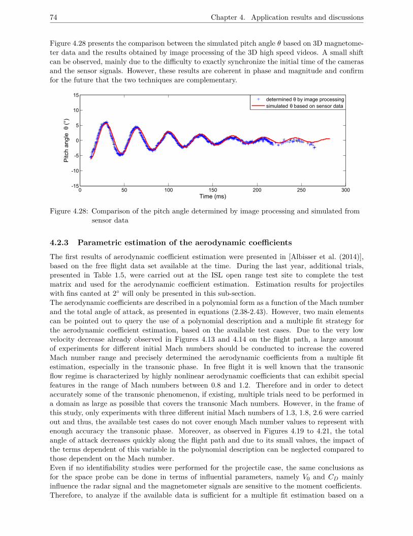
74 Chapter 4. Application results and discussions
Figure 4.28 presents the comparison between the simulated pitch angle θ based on 3D magnetome-ter data and the results obtained by image processing of the 3D high speed videos. A small shiftcan be observed, mainly due to the difficulty to exactly synchronize the initial time of the camerasand the sensor signals. However, these results are coherent in phase and magnitude and confirmfor the future that the two techniques are complementary.
0 50 100 150 200 250 300-15
-10
-5
0
5
10
15
Pitc
h an
gleθ
(°)
Time (ms)
determined θ by image processingsimulated θ based on sensor data
Figure 4.28: Comparison of the pitch angle determined by image processing and simulated fromsensor data
4.2.3 Parametric estimation of the aerodynamic coefficients
The first results of aerodynamic coefficient estimation were presented in [Albisser et al. (2014)],based on the free flight data set available at the time. During the last year, additional trials,presented in Table 1.5, were carried out at the ISL open range test site to complete the testmatrix and used for the aerodynamic coefficient estimation. Estimation results for projectileswith fins canted at 2◦ will only be presented in this sub-section.The aerodynamic coefficients are described in a polynomial form as a function of the Mach numberand the total angle of attack, as presented in equations (2.38-2.43). However, two main elementscan be pointed out to query the use of a polynomial description and a multiple fit strategy forthe aerodynamic coefficient estimation, based on the available test cases. Due to the very lowvelocity decrease already observed in Figures 4.13 and 4.14 on the flight path, a large amountof experiments for different initial Mach numbers should be conducted to increase the coveredMach number range and precisely determined the aerodynamic coefficients from a multiple fitestimation, especially in the transonic phase. In free flight it is well known that the transonicflow regime is characterized by highly nonlinear aerodynamic coefficients that can exhibit specialfeatures in the range of Mach numbers between 0.8 and 1.2. Therefore and in order to detectaccurately some of the transonic phenomenon, if existing, multiple trials need to be performed ina domain as large as possible that covers the transonic Mach numbers. However, in the frame ofthis study, only experiments with three different initial Mach numbers of 1.3, 1.8, 2.6 were carriedout and thus, the available test cases do not cover enough Mach number values to represent withenough accuracy the transonic phase. Moreover, as observed in Figures 4.19 to 4.21, the totalangle of attack decreases quickly along the flight path and due to its small values, the impact ofthe terms dependent of this variable in the polynomial description can be neglected compared tothose dependent on the Mach number.Even if no identifiability studies were performed for the projectile case, the same conclusions asfor the space probe can be done in terms of influential parameters, namely V0 and CD mainlyinfluence the radar signal and the magnetometer signals are sensitive to the moment coefficients.Therefore, to analyze if the available data is sufficient for a multiple fit estimation based on a
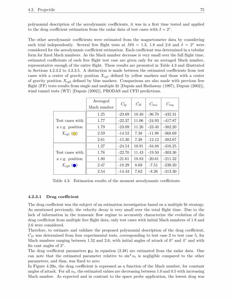
4.2. Projectile 75
polynomial description of the aerodynamic coefficients, it was in a first time tested and appliedto the drag coefficient estimation from the radar data of test cases with δ = 2◦.
The other aerodynamic coefficients were estimated from the magnetometer data by consideringeach trial independently. Several free flight tests at M0 = 1.3, 1.8 and 2.6 and δ = 2◦ wereconsidered for the aerodynamic coefficient estimation. Each coefficient was determined in a tabularform for fixed Mach numbers. As the Mach number decrease is very small over the full flight time,estimated coefficients of each free flight test case are given only for an averaged Mach number,representative enough of the entire flight. These results are presented in Table 4.3 and illustratedin Sections 4.2.3.2 to 4.2.3.5. A distinction is made between the estimated coefficients from testcases with a center of gravity position Xcg1 defined by yellow markers and those with a centerof gravity position Xcg2 defined by blue markers. Comparisons are also made with previous freeflight (FF) tests results from single and multiple fit [Dupuis and Hathaway (1997), Dupuis (2002)],wind tunnel tests (WT) [Dupuis (2002)], PRODAS and CFD predictions.
AveragedMach number
Clp Clδ Cmα Cmq
1.25 -23.69 10.40 -36.70 -432.31Test cases with 1.77 -22.37 11.06 -24.93 -417.87a c.g. position 1.79 -23.09 11.26 -23.40 -382.20Xcg1 ( ) 2.59 -14.52 7.38 -11.98 -368.69
2.61 -15.30 7.38 -12.12 -382.671.27 -24.54 10.91 -34.88 -316.25
Test cases with 1.76 -22.70 11.43 -19.50 -303.36a c.g. position 1.80 -21.61 10.83 -20.61 -211.32Xcg2 ( ) 2.47 -18.29 8.69 -7.51 -239.20
2.54 -14.43 7.62 -8.26 -313.30
Table 4.3: Estimation results of the moment aerodynamic coefficients
4.2.3.1 Drag coefficient
The drag coefficient was the subject of an estimation investigation based on a multiple fit strategy.As mentioned previously, the velocity decay is very small over the total flight time. Due to thelack of information in the transonic flow regime to accurately characterize the evolution of thedrag coefficient from multiple free flight data, only test cases with initial Mach numbers of 1.8 and2.6 were considered.Therefore, to estimate and validate the proposed polynomial description of the drag coefficient,CD was determined from four experimental tests, corresponding to test case 2 to test case 5, forMach numbers ranging between 1.52 and 2.6, with initial angles of attack of 0◦ and 4◦ and withfin cant angles of 2◦.The drag coefficient parameters pD in equation (2.38) are estimated from the radar data. Onecan note that the estimated parameter relative to sin4 αt is negligible compared to the otherparameters, and thus, was fixed to zero.In Figure 4.29a, the drag coefficient is expressed as a function of the Mach number, for constantangles of attack. For all αt, the estimated values are decreasing between 1.0 and 0.5 with increasingMach number. As expected and in contrast to the space probe application, the lowest drag was
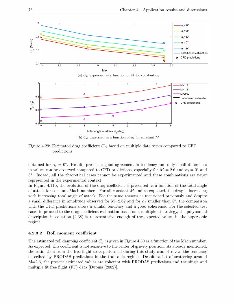
76 Chapter 4. Application results and discussions
1.3 1.5 1.7 1.9 2.1 2.3 2.5 2.70.4
0.6
0.8
1
Mach
CD(Mach)
CFD predictions
data-based estimation
αt = 9°
αt = 7°
αt = 5°
αt = 3°
αt = 0°
(a) CD expressed as a function of M for constant αt
0 1 2 3 4 5 6 7 8 90.4
0.6
0.8
1
Total angle of attack αt(deg)
CD(αt)
M=1.3
M=1.8
M=2.62
CFD predictions
data-based estimation
(b) CD expressed as a function of αt for constant M
Figure 4.29: Estimated drag coefficient CD based on multiple data series compared to CFDpredictions
obtained for αt = 0◦. Results present a good agreement in tendency and only small differencesin values can be observed compared to CFD predictions, especially for M = 2.6 and αt = 0◦ and3◦. Indeed, all the theoretical cases cannot be experimented and these combinations are neverrepresented in the experimental context.In Figure 4.11b, the evolution of the drag coefficient is presented as a function of the total angleof attack for constant Mach numbers. For all constant M and as expected, the drag is increasingwith increasing total angle of attack. For the same reasons as mentioned previously and despitea small difference in amplitude observed for M=2.62 and for αt smaller than 5◦, the comparisonwith the CFD predictions shows a similar tendency and a good coherence. For the selected testcases to proceed to the drag coefficient estimation based on a multiple fit strategy, the polynomialdescription in equation (2.38) is representative enough of the expected values in the supersonicregime.
4.2.3.2 Roll moment coefficient
The estimated roll damping coefficient Clp is given in Figure 4.30 as a function of the Mach number.As expected, this coefficient is not sensitive to the center of gravity position. As already mentioned,the estimation from the free flight tests performed during this study cannot reveal the tendencydescribed by PRODAS predictions in the transonic regime. Despite a bit of scattering aroundM=2.6, the present estimated values are coherent with PRODAS predictions and the single andmultiple fit free flight (FF) data [Dupuis (2002)].
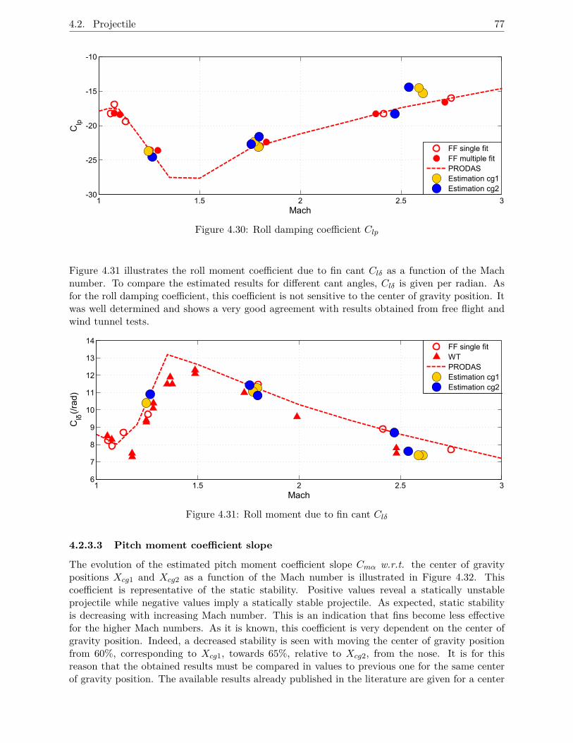
4.2. Projectile 77
1 1.5 2 2.5 3-30
-25
-20
-15
-10
Mach
Clp
FF single fitFF multiple fitPRODASEstimation cg1Estimation cg2
Figure 4.30: Roll damping coefficient Clp
Figure 4.31 illustrates the roll moment coefficient due to fin cant Clδ as a function of the Machnumber. To compare the estimated results for different cant angles, Clδ is given per radian. Asfor the roll damping coefficient, this coefficient is not sensitive to the center of gravity position. Itwas well determined and shows a very good agreement with results obtained from free flight andwind tunnel tests.
1 1.5 2 2.5 36
7
8
9
10
11
12
13
14
Mach
Clδm/rado
FF single fitWTPRODASEstimation cg1Estimation cg2
Figure 4.31: Roll moment due to fin cant Clδ
4.2.3.3 Pitch moment coefficient slope
The evolution of the estimated pitch moment coefficient slope Cmα w.r.t. the center of gravitypositions Xcg1 and Xcg2 as a function of the Mach number is illustrated in Figure 4.32. Thiscoefficient is representative of the static stability. Positive values reveal a statically unstableprojectile while negative values imply a statically stable projectile. As expected, static stabilityis decreasing with increasing Mach number. This is an indication that fins become less effectivefor the higher Mach numbers. As it is known, this coefficient is very dependent on the center ofgravity position. Indeed, a decreased stability is seen with moving the center of gravity positionfrom 60%, corresponding to Xcg1, towards 65%, relative to Xcg2, from the nose. It is for thisreason that the obtained results must be compared in values to previous one for the same centerof gravity position. The available results already published in the literature are given for a center
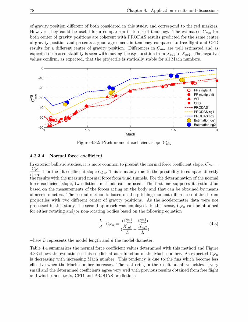
78 Chapter 4. Application results and discussions
of gravity position different of both considered in this study, and correspond to the red markers.However, they could be useful for a comparison in terms of tendency. The estimated Cmα forboth center of gravity positions are coherent with PRODAS results predicted for the same centerof gravity position and presents a good agreement in tendency compared to free flight and CFDresults for a different center of gravity position. Differences in Cmα are well estimated and asexpected decreased stability is seen with moving the c.g. position from Xcg1 to Xcg2. The negativevalues confirm, as expected, that the projectile is statically stable for all Mach numbers.
1 1.5 2 2.5 3-60
-50
-40
-30
-20
-10
0
Mach
Cmα
cg
FF single fitFF multiple fitWTCFDPRODASPRODAS cg1PRODAS cg2Estimation cg1Estimation cg2
Figure 4.32: Pitch moment coefficient slope Ccgmα
4.2.3.4 Normal force coefficient
In exterior ballistic studies, it is more common to present the normal force coefficient slope, CNα =CN
sinα than the lift coefficient slope CLα. This is mainly due to the possibility to compare directlythe results with the measured normal force from wind tunnels. For the determination of the normalforce coefficient slope, two distinct methods can be used. The first one supposes its estimationbased on the measurements of the forces acting on the body and that can be obtained by meansof accelerometers. The second method is based on the pitching moment difference obtained fromprojectiles with two different center of gravity positions. As the accelerometer data were notprocessed in this study, the second approach was employed. In this sense, CNα can be obtainedfor either rotating and/or non-rotating bodies based on the following equation
L
d· CNα = (Ccg1mα − Ccg2mα)
(Xcg1L− Xcg2
L)
(4.3)
where L represents the model length and d the model diameter.
Table 4.4 summarizes the normal force coefficient values determined with this method and Figure4.33 shows the evolution of this coefficient as a function of the Mach number. As expected CNαis decreasing with increasing Mach number. This tendency is due to the fins which become lesseffective when the Mach number increases. The scattering in the results at all velocities is verysmall and the determined coefficients agree very well with previous results obtained from free flightand wind tunnel tests, CFD and PRODAS predictions.
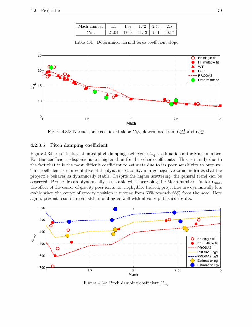
4.2. Projectile 79
Mach number 1.1 1.59 1.72 2.45 2.5CNα 21.04 13.03 11.13 9.01 10.17
Table 4.4: Determined normal force coefficient slope
1 1.5 2 2.5 35
10
15
20
25
Mach
CNα
FFAsingleAfitFFAmultipleAfitWTCFDPRODASDetermination
Figure 4.33: Normal force coefficient slope CNα determined from Ccg1mα and Ccg2mα
4.2.3.5 Pitch damping coefficient
Figure 4.34 presents the estimated pitch damping coefficient Cmq as a function of the Mach number.For this coefficient, dispersions are higher than for the other coefficients. This is mainly due tothe fact that it is the most difficult coefficient to estimate due to its poor sensitivity to outputs.This coefficient is representative of the dynamic stability: a large negative value indicates that theprojectile behaves as dynamically stable. Despite the higher scattering, the general trend can beobserved. Projectiles are dynamically less stable with increasing the Mach number. As for Cmα,the effect of the center of gravity position is not negligible. Indeed, projectiles are dynamically lessstable when the center of gravity position is moving from 60% towards 65% from the nose. Hereagain, present results are consistent and agree well with already published results.
1 1.5 2 2.5 3-700
-600
-500
-400
-300
-200
Mach
Cm
q
FFOsingleOfitFFOmultipleOfitPRODASPRODASOcg1PRODASOcg2EstimationOcg1EstimationOcg2
Figure 4.34: Pitch damping coefficient Cmq

80 Chapter 4. Application results and discussions
4.3 Discussions
In this chapter, several results have been described for a space probe and a projectile. Comparisonsbetween simulated and measured signals, parameter estimation results, as well as the evolution ofstate variables have been presented. The aerodynamic characteristics for the space probe and theprojectile present several differences. Both architectures have their own behaviour in flight thatcan be highlighted:
• velocity and drag coefficient: the space vehicle velocity decreases very quickly along the flightpath while the projectile velocity decay is very small. These results reveals higher drag valuesfor the space probe than for the projectile, as seen in Sections 4.1.3.1 and 4.2.3.1. Indeed,the order of magnitude of the drag coefficient for the space probe is almost two to threetimes higher than for the projectile. Also for the space probe, the drag is decreasing withincreasing total angle of attack while it is increasing for projectile;
• total angle of attack: for the space vehicle, the total angle of attack αt is usually increasingalong the flight path whereas αt is decreasing for the projectile. For the first model, thisvariable can reach angles higher than 20◦ depending on the test case. For the second model,the order of magnitude of αt is equivalent to the initial angle of attack α0 and it tends todecrease during the flight until values close to zero. These evolutions can be representativeof the stability of both models;
• dynamic stability: the dynamic stability, represented by negative values of the pitch dampingcoefficient Cmq, is satisfied only for specific Mach numbers and total angles of attack asseen in Section 4.1.3.2. For projectiles, it is well-known that this model is perfectly stabledynamically and this was confirmed by the results shown in Figure 4.34.
• spin rate: for equivalent velocities, even if a spin is induced for the space probe, the roll rateis clearly not comparable to the projectile with canted fins;
The obtained results are perfectly coherent with a priori knowledge in the exterior ballistic do-main and already published results in the literature, from wind tunnel measurements and/oraerodynamic predictions codes. Therefore, the developed code for the aerodynamic coefficient de-termination takes into account enough relevant effects to be representative of the real behaviourin flight and can be used for both architectures.The proposed multiple fit strategy for the parameter estimation has improved the physical inter-pretability of the coefficients depending on Mach numbers and total angles of attack. The identifiedcoefficients were validated for both architectures over a large range of variation of M and αt. Theaerodynamic coefficient estimation results based on a multiple fit strategy presented herein areconsistent with the ones obtained previously for similar configurations. For the space probe, theyessentially show that the drag coefficient is represented by a function of the Mach number and thetotal angle of attack with a coupling term in both variables. The pitch damping coefficient is acomplex function not only of the total angle of attack, but also of the Mach number.For the projectile, only the drag coefficient was the subject of a multiple fit strategy and CD ismainly described as a function of the Mach number and slightly influenced by a term in αt. Forthe remaining aerodynamic coefficients, a dependence only w.r.t. Mach numbers is representativeenough of the coefficient evolution.
Conclusions and perspectives
The work presented in this thesis is associated to the exterior ballistic framework. This domainaims at studying and understanding the behaviour of a vehicle in flight through the aerodynamiccoefficients characterizing it. Several complementary tools can be used to quantify the aerody-namic parameters. However, free flight tests are considered as reference because they allow tostudy the vehicle behaviour in flight under real conditions. This research subject deals with theidentification of aerodynamic coefficients from free flight data. To bring this project to a successfulend, the proposed approach consisted in a wise merging between the experimental context and theidentification techniques. Thus, an identification procedure was defined to guide the aerodynamicparameter estimation, composed of several steps, from the modelling of the behaviour of a vehiclein free flight to the aerodynamic parameter estimation.
The determination of aerodynamic characteristics remains dependent of the quality and quantityof the data obtained experimentally. Therefore, the study choices are mainly guided by the ex-perimental conditions and the available data. Chapter 1 described the experimental context fromthe design and conception of the two different model configurations, an Earth re-entry space ve-hicle and a fin-stabilized projectile, to the free flight tests. In terms of experimental conditions,only the initial Mach number and initial angle of attack can be defined. With the support of theskills at ISL, the expertise necessary for the experimental part is essential to obtain free flightdata by means of different measurement techniques. In the present study, they are precisely theradar and three-axis magnetometer measurements, collected by using two different data acquisitionapproaches, depending on the studied vehicle.
The proposed identification procedure allows to define a guideline of the studies to manage. Chap-ter 2 presented the first step of the identification procedure that consists in the physical modelling.The behaviour of a vehicle in flight is expressed as a six degrees of freedom nonlinear state-spacerepresentation. The general model structure is obtained from flight mechanics laws. Our interestwas mainly focused on the descriptions of the aerodynamic coefficients integrated in the modeland adapted to each application. Some descriptions already exist in the literature and in order tokeep a physical meaning of the parameters, polynomial descriptions as function of Mach numbersand total angles of attack were selected. However after multiple preliminary identification tests,we concluded that they do not reveal enough information of the aerodynamic coefficient evolution.With the purpose of keeping a physical meaning of the parameters, a modified aerodynamic coeffi-cient model was suggested with coupled dependency in state variables and spline functions. In thissense, the model was constructed from a grey-box approach with the integration of parametrizedfunctions describing the aerodynamic coefficients, where the parameters must be estimated fromfree flight data. The chosen model structure was implemented in the developed inverse 6DOF
82 Conclusions and perspectives
code, where initial conditions of the state variables and parameters describing the aerodynamiccoefficients can be estimated from free flight data.
The determination of aerodynamic parameters based on measured data is an inverse problemwhich can be impossible to solve if it is ill posed or difficult to solve if it is ill conditioned. Thatinvolves several identifiability tests of a unknown parameter set composed of the initial conditionsand the model parameters, to ensure that they can be estimated from the chosen model structureand the available data. These studies correspond to the a priori and a posteriori identifiabilityanalyses, respectively. They represent a major step of the identification procedure presented inChapter 3. These analyses were performed for the space vehicle case and a priori identifiabilityconcluded to a well-posed model structure. A posteriori identifiability analysis managed throughsensitivity analysis allows to guide the parameter estimation, and mainly highlights the most rel-evant parameters which can be determined from free flight data. This task is not easy in the caseof nonlinear models, where only local results can be obtained, hence the requirement of having aphysical representation of the behaviour of a vehicle in free flight and a priori knowledge. Suchinformation allows to know nonlinear functional relations between parameters, to impose initialguess of the parameters and interpret the obtain results. It was shown that using a priori knowl-edge of the system increases the number of identifiable initial conditions of the state variables.Concerning the a posteriori identifiability of the parameters describing the aerodynamic coeffi-cients, it revealed that the number of identifiable parameters increases when several free flighttests are considered. This conclusion is coherent with the a priori knowledge, as free flight testswere managed for different initial experimental conditions in order to have distinct behaviours inflight, mainly in terms of total angle of attack evolution. Taking into account the identifiabilityresults, the estimation was divided in two steps: the first one meant to determine essentially thestate variable initial conditions for each test separately, while the second step proposed to estimatethe aerodynamic coefficients through a multiple fit strategy. This approach, successfully appliedto both applications, enabled to characterize the coefficients on a larger range of flight conditions.
Chapter 4 presented and discussed the main results of aerodynamic coefficient estimation basedon single and/or multiple fit strategy, as well as the evolution of the output signals and the statevariables. For the space probe case, the drag and pitch damping coefficients were described in apolynomial form as function of the Mach number and the total angle of attack. Guided by theidentifiability analysis, the model parameters were estimated from a multiple fit strategy. Forthe projectile, the experimental conditions and available data are limited in terms of range ofvariation of the Mach number and the total angle of attack. Therefore, this makes it difficult todescribe the aerodynamic coefficients in a polynomial form, analyze the identifiability and estimatethe model parameters from multiple fit strategy. For this reason and as preliminary testing,only the drag coefficient was described as a function of the Mach number and the total angleof attack. The parameters were determined from a multiple fit strategy only in the supersonicflow regime. The other aerodynamic coefficients were estimated in a tabular form for constantMach numbers and by considering each trial independently. For both applications, estimationresults compare well with the results obtained previously for similar configurations. Moreover,simulated and measured output signals present a very good agreement after state variable initialconditions and aerodynamic coefficient estimation, that reinforces the employed procedure for theparameter identification and the ability of the model to reproduce the measured output signals. Forprojectiles, very good agreement is observed for results obtained from the different measurementstechniques, namely the axial position and the pitch angle from radar data and on-board sensortechnique, respectively, compared to high speed trajectory tracker system. This complementarymeasurement technique allows to validate our results by comparison with those obtained by imageprocessing on 3D high speed videos. To justify the difference of behaviour in flight of these two
Conclusions and perspectives 83
vehicles, a comparison between the Earth re-entry space vehicle and projectile was done, in termsof aerodynamic characteristics and their variable evolutions.
The different studies in the frame of this thesis mainly led to scientific contributions in the ex-terior ballistic domain through the development of an identification procedure. This allowed theimplementation of a new inverse 6DOF code, Inv6DoF, to identify aerodynamic characteristicsfrom free flight data, including:
• a model structure characterizing precisely the behaviour of a vehicle in free flight;
• a complete descriptions of the aerodynamic coefficients as a function of the Mach number andthe total angle of attack, especially for the space probe where the drag and the pitch dampingcoefficients are described with coupled state variables and spline functions, respectively;
• the sensitivity functions to evaluate the parameter identifiability from single or multiple dataseries;
• an estimation code to determine the aerodynamic coefficients from a single or a multiple fitstrategy.
Perspectives
In the continuity of the present investigations, future works can be suggested.
It could be useful to extend the works dealing with the identification procedure, so far only testedfor two configurations. It could also be adapted to other architectures, such as gyro-stabilisedprojectiles.
An interesting area of study would be the analysis of the behaviour of a vehicle in flight in thetransonic flow regimes, especially for the Basic Finner projectile. It is characterized by highlynonlinear aerodynamic coefficients that can exhibit special features in the range of Mach numbersbetween 0.8 and 1.2. Moreover, the assumption of negligible aerodynamic coefficients, for examplethe Magnus moment coefficient slope, is generally no longer valid in transonic regime and thesecoefficients should be integrated in the modelling step.
Concerning the measurement techniques, the use of accelerometers will enable to have access toinformation about the forces acting on the vehicle. In addition, the promising results obtainedby image processing from 3D high speed video encourage us to continue our studies, especially interms of lateral position and yaw angle determination.
The longer term objective of this work is to combine the identification techniques with controltools. In that respect, we are currently exploring several descriptions of the nonlinear dynamicssystem of a vehicle in flight such as a Linear Parameter Varying (LPV) model [Marcos (2001),Fujimori and Ljung (2006), Toth (2010), Theodoulis et al. (2010)]. This choice of modelling ismotivated by the fact that the use of LPV design techniques could ease the integration of LPVcontroller in the case of guided vehicle. Taking into account that the parameters have a physicalinterpretation, it would be interesting to use an LPV state-space representation.This would requirethe use of more complex identification method [Mercere (2012), Laroche et al. (2011), Wills andNinness (2011), Verdult et al. (2004)] but several issues are still open.

84 Conclusions and perspectives
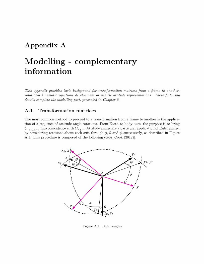
Appendix A
Modelling - complementaryinformation
This appendix provides basic background for transformation matrices from a frame to another,rotational kinematic equations development or vehicle attitude representations. These followingdetails complete the modelling part, presented in Chapter 2.
A.1 Transformation matrices
The most common method to proceed to a transformation from a frame to another is the applica-tion of a sequence of attitude angle rotations. From Earth to body axes, the purpose is to bringOxE ,yE ,zE into coincidence with Ox,y,z. Attitude angles are a particular application of Euler angles,by considering rotations about each axis through φ, θ and ψ successively, as described in FigureA.1. This procedure is composed of the following steps [Cook (2012)]:
O
q
y
f
xE
x1
x2 , xyE
y1 , y2
y
zz2
zE , z1
q
f
y
Figure A.1: Euler angles
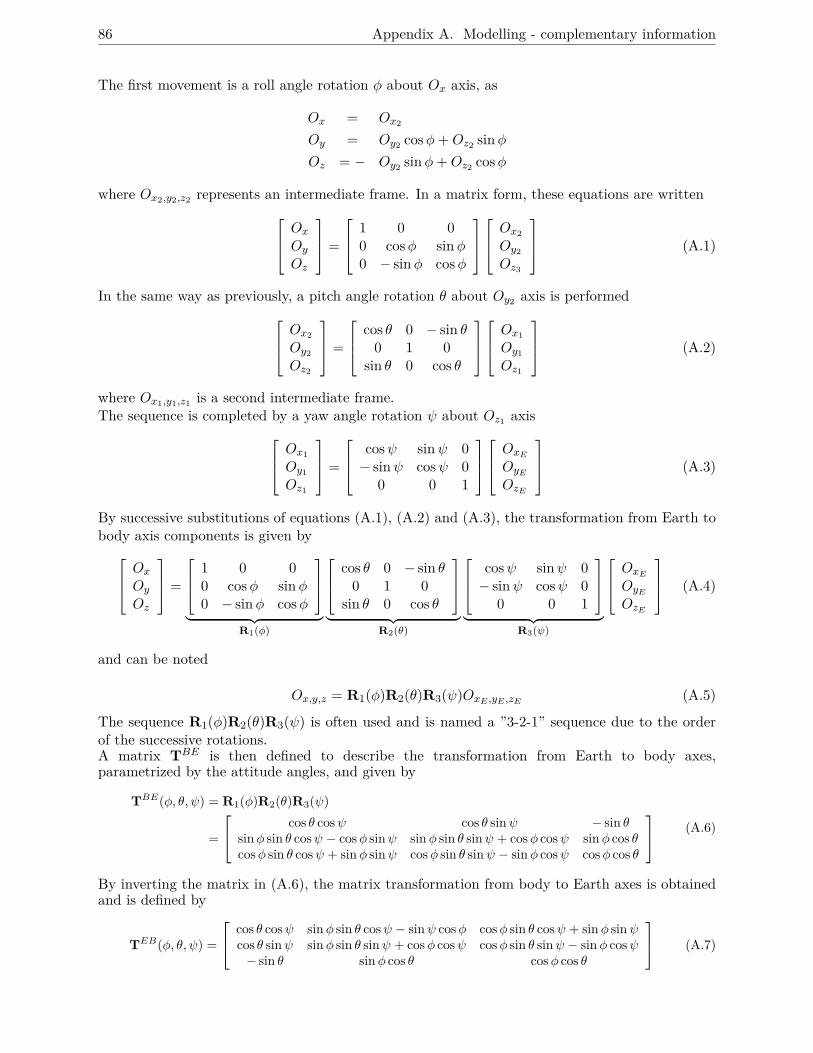
86 Appendix A. Modelling - complementary information
The first movement is a roll angle rotation φ about Ox axis, as
Ox = Ox2
Oy = Oy2 cosφ+Oz2 sinφOz = − Oy2 sinφ+Oz2 cosφ
where Ox2,y2,z2 represents an intermediate frame. In a matrix form, these equations are written OxOyOz
=
1 0 00 cosφ sinφ0 − sinφ cosφ
Ox2
Oy2
Oz3
(A.1)
In the same way as previously, a pitch angle rotation θ about Oy2 axis is performed Ox2
Oy2
Oz2
=
cos θ 0 − sin θ0 1 0
sin θ 0 cos θ
Ox1
Oy1
Oz1
(A.2)
where Ox1,y1,z1 is a second intermediate frame.The sequence is completed by a yaw angle rotation ψ about Oz1 axis Ox1
Oy1
Oz1
=
cosψ sinψ 0− sinψ cosψ 0
0 0 1
OxEOyEOzE
(A.3)
By successive substitutions of equations (A.1), (A.2) and (A.3), the transformation from Earth tobody axis components is given by Ox
OyOz
=
1 0 00 cosφ sinφ0 − sinφ cosφ
︸ ︷︷ ︸
R1(φ)
cos θ 0 − sin θ0 1 0
sin θ 0 cos θ
︸ ︷︷ ︸
R2(θ)
cosψ sinψ 0− sinψ cosψ 0
0 0 1
︸ ︷︷ ︸
R3(ψ)
OxEOyEOzE
(A.4)
and can be noted
Ox,y,z = R1(φ)R2(θ)R3(ψ)OxE ,yE ,zE (A.5)
The sequence R1(φ)R2(θ)R3(ψ) is often used and is named a ”3-2-1” sequence due to the orderof the successive rotations.A matrix TBE is then defined to describe the transformation from Earth to body axes,parametrized by the attitude angles, and given by
TBE(φ, θ, ψ) = R1(φ)R2(θ)R3(ψ)
=
cos θ cosψ cos θ sinψ − sin θsinφ sin θ cosψ − cosφ sinψ sinφ sin θ sinψ + cosφ cosψ sinφ cos θcosφ sin θ cosψ + sinφ sinψ cosφ sin θ sinψ − sinφ cosψ cosφ cos θ
(A.6)
By inverting the matrix in (A.6), the matrix transformation from body to Earth axes is obtainedand is defined by
TEB(φ, θ, ψ) =
cos θ cosψ sinφ sin θ cosψ − sinψ cosφ cosφ sin θ cosψ + sinφ sinψcos θ sinψ sinφ sin θ sinψ + cosφ cosψ cosφ sin θ sinψ − sinφ cosψ− sin θ sinφ cos θ cosφ cos θ
(A.7)
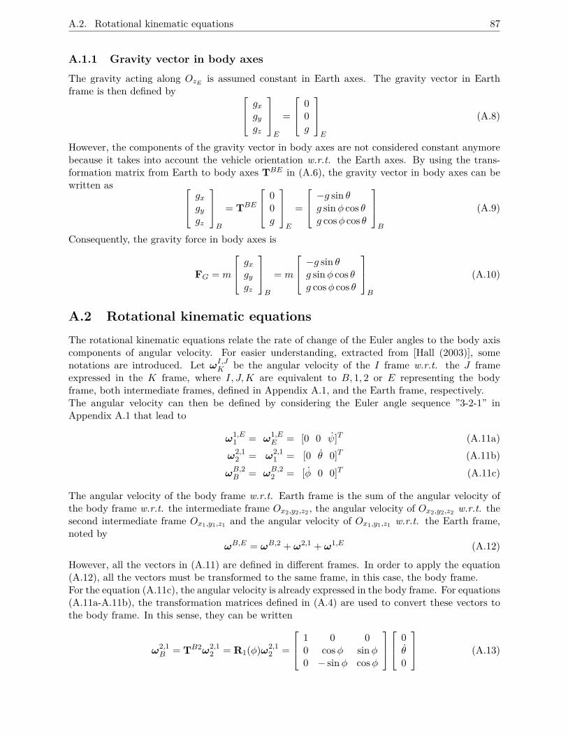
A.2. Rotational kinematic equations 87
A.1.1 Gravity vector in body axes
The gravity acting along OzE is assumed constant in Earth axes. The gravity vector in Earthframe is then defined by gx
gygz
E
=
00g
E
(A.8)
However, the components of the gravity vector in body axes are not considered constant anymorebecause it takes into account the vehicle orientation w.r.t. the Earth axes. By using the trans-formation matrix from Earth to body axes TBE in (A.6), the gravity vector in body axes can bewritten as gx
gygz
B
= TBE
00g
E
=
−g sin θg sinφ cos θg cosφ cos θ
B
(A.9)
Consequently, the gravity force in body axes is
FG = m
gxgygz
B
= m
−g sin θg sinφ cos θg cosφ cos θ
B
(A.10)
A.2 Rotational kinematic equations
The rotational kinematic equations relate the rate of change of the Euler angles to the body axiscomponents of angular velocity. For easier understanding, extracted from [Hall (2003)], somenotations are introduced. Let ωI,JK be the angular velocity of the I frame w.r.t. the J frameexpressed in the K frame, where I, J,K are equivalent to B, 1, 2 or E representing the bodyframe, both intermediate frames, defined in Appendix A.1, and the Earth frame, respectively.The angular velocity can then be defined by considering the Euler angle sequence ”3-2-1” inAppendix A.1 that lead to
ω1,E1 = ω1,E
E = [0 0 ψ]T (A.11a)ω2,1
2 = ω2,11 = [0 θ 0]T (A.11b)
ωB,2B = ωB,22 = [φ 0 0]T (A.11c)
The angular velocity of the body frame w.r.t. Earth frame is the sum of the angular velocity ofthe body frame w.r.t. the intermediate frame Ox2,y2,z2 , the angular velocity of Ox2,y2,z2 w.r.t. thesecond intermediate frame Ox1,y1,z1 and the angular velocity of Ox1,y1,z1 w.r.t. the Earth frame,noted by
ωB,E = ωB,2 + ω2,1 + ω1,E (A.12)
However, all the vectors in (A.11) are defined in different frames. In order to apply the equation(A.12), all the vectors must be transformed to the same frame, in this case, the body frame.For the equation (A.11c), the angular velocity is already expressed in the body frame. For equations(A.11a-A.11b), the transformation matrices defined in (A.4) are used to convert these vectors tothe body frame. In this sense, they can be written
ω2,1B = TB2ω2,1
2 = R1(φ)ω2,12 =
1 0 00 cosφ sinφ0 − sinφ cosφ
0θ0
(A.13)
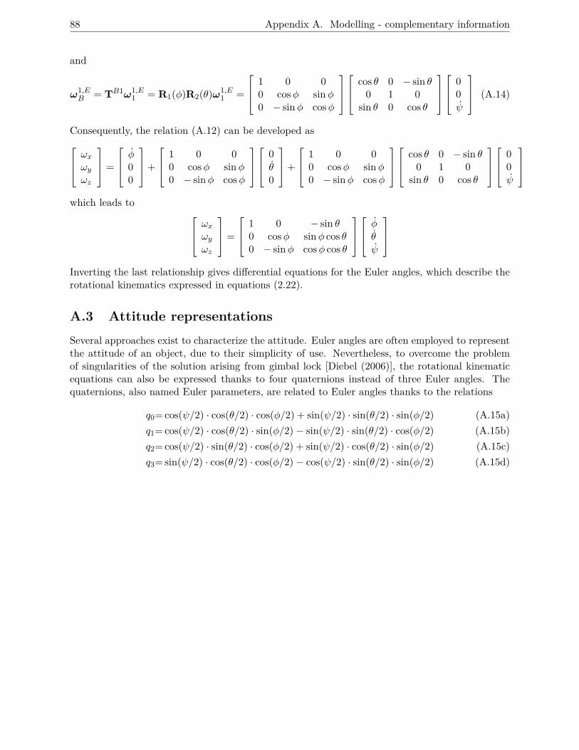
88 Appendix A. Modelling - complementary information
and
ω1,EB = TB1ω1,E
1 = R1(φ)R2(θ)ω1,E1 =
1 0 00 cosφ sinφ0 − sinφ cosφ
cos θ 0 − sin θ
0 1 0sin θ 0 cos θ
0
0ψ
(A.14)
Consequently, the relation (A.12) can be developed as ωxωyωz
=
φ00
+
1 0 00 cosφ sinφ0 − sinφ cosφ
0θ0
+
1 0 00 cosφ sinφ0 − sinφ cosφ
cos θ 0 − sin θ
0 1 0sin θ 0 cos θ
0
0ψ
which leads to ωx
ωyωz
=
1 0 − sin θ0 cosφ sinφ cos θ0 − sinφ cosφ cos θ
φ
θ
ψ
Inverting the last relationship gives differential equations for the Euler angles, which describe therotational kinematics expressed in equations (2.22).
A.3 Attitude representations
Several approaches exist to characterize the attitude. Euler angles are often employed to representthe attitude of an object, due to their simplicity of use. Nevertheless, to overcome the problemof singularities of the solution arising from gimbal lock [Diebel (2006)], the rotational kinematicequations can also be expressed thanks to four quaternions instead of three Euler angles. Thequaternions, also named Euler parameters, are related to Euler angles thanks to the relations
q0= cos(ψ/2) · cos(θ/2) · cos(φ/2) + sin(ψ/2) · sin(θ/2) · sin(φ/2) (A.15a)q1= cos(ψ/2) · cos(θ/2) · sin(φ/2)− sin(ψ/2) · sin(θ/2) · cos(φ/2) (A.15b)q2= cos(ψ/2) · sin(θ/2) · cos(φ/2) + sin(ψ/2) · cos(θ/2) · sin(φ/2) (A.15c)q3= sin(ψ/2) · cos(θ/2) · cos(φ/2)− cos(ψ/2) · sin(θ/2) · sin(φ/2) (A.15d)
Appendix B
Static and dynamic stability
This appendix defines the static and dynamic stability in an aeroballistic sense in order to linkthese notions to the stability as defined in automatic control.
The static and dynamic stability are defined as follows:Static stability refers to whether the initial tendency of the vehicle response to a perturbation istoward a restoration of equilibrium. For example, if the response to an infinitesimal increase in an-gle of attack α generates a pitching moment Cm that reduces the angle of attack, the configurationis said to be statically stable to such perturbations. Without static stability, a small perturbationfrom the trimmed (steady state) angle of attack would continue to increase in magnitude andcould induce the tumbling of the vehicle [Strickland (2010)]. The static stability is associated tothe pitch moment coefficient slope Cmα = ∂Cm/∂α. This derivative describes the rate of change ofthe pitching moment coefficient with angle of attack and static stability is ensured with negativevalues of Cmα.
Dynamic stability refers to whether the vehicle ultimately returns to the initial equilibrium stateafter some infinitesimal perturbations. Consideration of dynamic stability makes sense only forvehicles that are statically stable. But a vehicle can be statically stable and dynamically unstable(for example, if the initial tendency to return toward equilibrium leads to an overshoot, it ispossible to have a oscillatory divergence of continuously increasing amplitude) [Caughey (2011)].The dynamic stability is associated to the pitch damping coefficient Cmq = ∂Cm/∂(ωyd2V ). Thisderivatives represents the rate of change of the pitching moment coefficient with angular velocityin pitch ωy with constant angle of attack and dynamic stability is ensured with negative values ofCmq. More precisely, the pitch damping coefficient has been treated as the sum of two individualcoefficients, Cmq and Cmα, that produce an aerodynamic moment proportional to the angular rateassociated with the angle of attack. In fact, these two individual coefficients represent momentsproportional to two different angular rates, α and ωy, that are associated with the angle of attackα and the the angular displacement of the longitudinal axis of the body w.r.t. the Earth-fixed axissystem denoted by θ, respectively. For many nonmaneuvering flight trajectories, including thoseflown in ballistic aerodynamic ranges and for rectilinear flight path, the angular rates α and ωy areequal and the moment expansion can be simplified by combining the two damping coefficient intoa single coefficient sum, which is proportional to a single angular rate [Weinacht (1998), McCoy(1999)].
To investigate the stability of a vehicle, the linearisation of the equations of motion allows totake advantage of linear stability criteria. Supposing the following linearized flight dynamic model
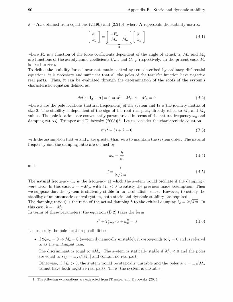
90 Appendix B. Static and dynamic stability
x = Ax obtained from equations (2.19b) and (2.21b), where A represents the stability matrix:[αωy
]=[−Fα 1Mα Mq
]︸ ︷︷ ︸
A
[αωy
](B.1)
where Fα is a function of the force coefficients dependent of the angle of attack α, Mα and Mq
are functions of the aerodynamic coefficients Cmα and Cmq, respectively. In the present case, Fαis fixed to zero.To define the stability for a linear automatic control system described by ordinary differentialequations, it is necessary and sufficient that all the poles of the transfer function have negativereal parts. Thus, it can be evaluated through the determination of the roots of the system’scharacteristic equation defined as:
det[s · I2 −A] = 0⇒ s2 −Mq · s−Mα = 0 (B.2)
where s are the pole locations (natural frequencies) of the system and I2 is the identity matrix ofsize 2. The stability is dependent of the sign of the root real part, directly relied to Mα and Mq
values. The pole locations are conveniently parametrized in terms of the natural frequency ωn anddamping ratio ζ [Trumper and Dubowsky (2005)] 1. Let us consider the characteristic equation
ms2 + bs+ k = 0 (B.3)
with the assumption that m and k are greater than zero to maintain the system order. The naturalfrequency and the damping ratio are defined by
ωn = k
m(B.4)
andζ = b
2√km
(B.5)
The natural frequency ωn is the frequency at which the system would oscillate if the damping bwere zero. In this case, k = −Mα, with Mα < 0 to satisfy the previous made assumption. Thenwe suppose that the system is statically stable in an aeroballistic sense. However, to satisfy thestability of an automatic control system, both static and dynamic stability are required.The damping ratio ζ is the ratio of the actual damping b to the critical damping bc = 2
√km. In
this case, b = −Mq.In terms of these parameters, the equation (B.2) takes the form
s2 + 2ζωn · s+ ω2n = 0 (B.6)
Let us study the pole location possibilities:
• if 2ζωn = 0⇒Mq = 0 (system dynamically unstable), it corresponds to ζ = 0 and is referredto as the undamped case.The discriminant is equal to 4Mα. The system is statically stable if Mα < 0 and the polesare equal to s1,2 = ±j
√|Mα| and contain no real part.
Otherwise, if Mα > 0, the system would be statically unstable and the poles s1,2 = ±√Mα
cannot have both negative real parts. Thus, the system is unstable.
1. The following explanations are extracted from [Trumper and Dubowsky (2005)].
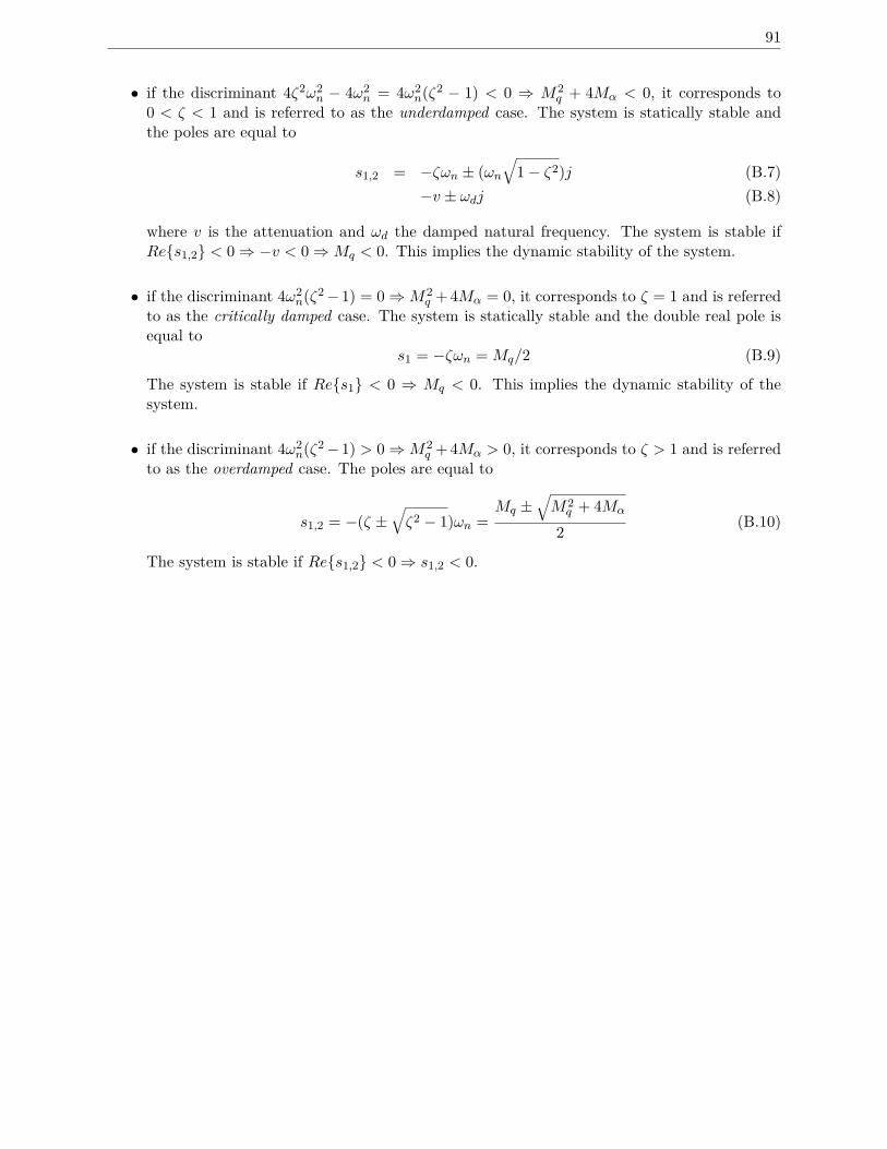
91
• if the discriminant 4ζ2ω2n − 4ω2
n = 4ω2n(ζ2 − 1) < 0 ⇒ M2
q + 4Mα < 0, it corresponds to0 < ζ < 1 and is referred to as the underdamped case. The system is statically stable andthe poles are equal to
s1,2 = −ζωn ± (ωn√
1− ζ2)j (B.7)−v ± ωdj (B.8)
where v is the attenuation and ωd the damped natural frequency. The system is stable ifRe{s1,2} < 0⇒ −v < 0⇒Mq < 0. This implies the dynamic stability of the system.
• if the discriminant 4ω2n(ζ2−1) = 0⇒M2
q + 4Mα = 0, it corresponds to ζ = 1 and is referredto as the critically damped case. The system is statically stable and the double real pole isequal to
s1 = −ζωn = Mq/2 (B.9)
The system is stable if Re{s1} < 0 ⇒ Mq < 0. This implies the dynamic stability of thesystem.
• if the discriminant 4ω2n(ζ2−1) > 0⇒M2
q + 4Mα > 0, it corresponds to ζ > 1 and is referredto as the overdamped case. The poles are equal to
s1,2 = −(ζ ±√ζ2 − 1)ωn =
Mq ±√M2q + 4Mα
2 (B.10)
The system is stable if Re{s1,2} < 0⇒ s1,2 < 0.

92 Appendix B. Static and dynamic stability
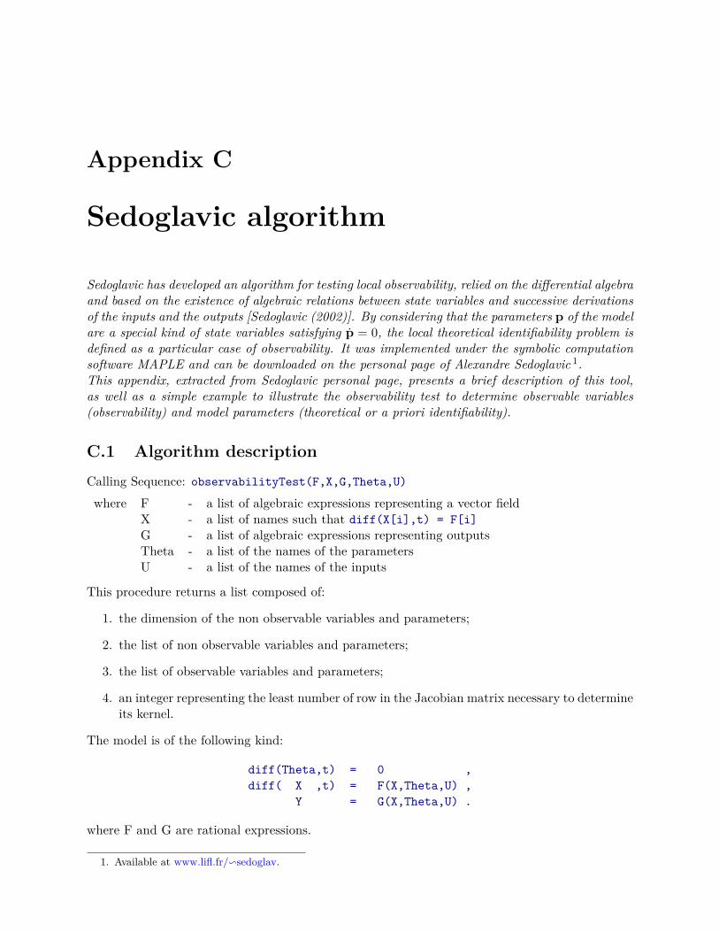
Appendix C
Sedoglavic algorithm
Sedoglavic has developed an algorithm for testing local observability, relied on the differential algebraand based on the existence of algebraic relations between state variables and successive derivationsof the inputs and the outputs [Sedoglavic (2002)]. By considering that the parameters p of the modelare a special kind of state variables satisfying p = 0, the local theoretical identifiability problem isdefined as a particular case of observability. It was implemented under the symbolic computationsoftware MAPLE and can be downloaded on the personal page of Alexandre Sedoglavic 1.This appendix, extracted from Sedoglavic personal page, presents a brief description of this tool,as well as a simple example to illustrate the observability test to determine observable variables(observability) and model parameters (theoretical or a priori identifiability).
C.1 Algorithm description
Calling Sequence: observabilityTest(F,X,G,Theta,U)where F - a list of algebraic expressions representing a vector field
X - a list of names such that diff(X[i],t) = F[i]
G - a list of algebraic expressions representing outputsTheta - a list of the names of the parametersU - a list of the names of the inputs
This procedure returns a list composed of:
1. the dimension of the non observable variables and parameters;
2. the list of non observable variables and parameters;
3. the list of observable variables and parameters;
4. an integer representing the least number of row in the Jacobian matrix necessary to determineits kernel.
The model is of the following kind:
diff(Theta,t) = 0 ,
diff( X ,t) = F(X,Theta,U) ,
Y = G(X,Theta,U) .
where F and G are rational expressions.
1. Available at www.lifl.fr/vsedoglav.
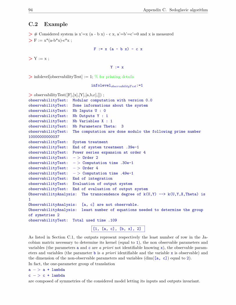
94 Appendix C. Sedoglavic algorithm
C.2 Example
> # Considered system is x’=x (a - b x) - c x, a’=b’=c’=0 and x is measured> F := x*(a-b*x)-c*x ;
F := x (a - b x) - c x
> Y := x ;
Y := x
> infolevel[observabilityTest] := 1; % for printing details
infolevelobservabilityTest:=1
> observabilityTest([F],[x],[Y],[a,b,c],[]) ;observabilityTest: Modular computation with version 0.0
observabilityTest: Some informations about the system
observabilityTest: Nb Inputs U : 0
observabilityTest: Nb Outputs Y : 1
observabilityTest: Nb Variables X : 1
observabilityTest: Nb Parameters Theta: 3
observabilityTest: The computation are done modulo the following prime number
10000000000037
observabilityTest: System treatment
observabilityTest: End of system treatment .39e-1
observabilityTest: Power series expansion at order 4
observabilityTest: − > Order 2
observabilityTest: − > Computation time .30e-1
observabilityTest: − > Order 4
observabilityTest: − > Computation time .49e-1
observabilityTest: End of integration
observabilityTest: Evaluation of output system
observabilityTest: End of evaluation of output system
ObservabilityAnalysis: The transcendence degree of k(U,Y) --> k(U,Y,X,Theta) is
1
ObservabilityAnalysis: [a, c] are not observable.
ObservabilityAnalysis: least number of equations needed to determine the group
of symetries 2
observabilityTest: Total used time .109
[1, [a, c], [b, x], 2]
As listed in Section C.1, the outputs represent respectively the least number of row in the Ja-cobian matrix necessary to determine its kernel (equal to 1), the non observable parameters andvariables (the parameters a and c are a priori not identifiable knowing x), the observable param-eters and variables (the parameter b is a priori identifiable and the variable x is observable) andthe dimension of the non-observable parameters and variables (dim([a, c]) equal to 2).In fact, the one-parameter group of translationa − > a + lambda
c − > c + lambda
are composed of symmetries of the considered model letting its inputs and outputs invariant.
List of Figures
Figure 1 Differentes possibilites pour quantifier les coefficients aerodynamiques . . 2
Figure 1.1 Schematic of a space probe configuration . . . . . . . . . . . . . . . . . . 11Figure 1.2 Schematic of the Basic Finner projectile . . . . . . . . . . . . . . . . . . . 12Figure 1.3 Sabot for a space probe model . . . . . . . . . . . . . . . . . . . . . . . . 13Figure 1.4 Sabot for a projectile . . . . . . . . . . . . . . . . . . . . . . . . . . . . . 14Figure 1.5 Electronic package of the space probe model . . . . . . . . . . . . . . . . 15Figure 1.6 Electronic package of the Basic Finner projectile . . . . . . . . . . . . . . 15Figure 1.7 Top-view of the open range test site . . . . . . . . . . . . . . . . . . . . . 17Figure 1.8 Spin adapter . . . . . . . . . . . . . . . . . . . . . . . . . . . . . . . . . . 18
Figure 2.1 Earth, body and wind frames . . . . . . . . . . . . . . . . . . . . . . . . . 22Figure 2.2 Representation of state variables of a space probe model . . . . . . . . . 24Figure 2.3 Global aerodynamic coefficients relied to forces and moments acting on a
projectile . . . . . . . . . . . . . . . . . . . . . . . . . . . . . . . . . . . . 25Figure 2.4 Euler angles . . . . . . . . . . . . . . . . . . . . . . . . . . . . . . . . . . 27Figure 2.5 Free-flight measurements of a spinning projectile (M0 = 2.63, α0 = 4◦,
δ = 2◦) . . . . . . . . . . . . . . . . . . . . . . . . . . . . . . . . . . . . . 36
Figure 3.1 Identification procedure . . . . . . . . . . . . . . . . . . . . . . . . . . . . 42Figure 3.2 Matlab/ Simulink block diagram . . . . . . . . . . . . . . . . . . . . . . . 43Figure 3.3 Classification of identifiability definitions, where M denotes the model
structure, u the input signals, tk the measurement times and vk the outputnoise . . . . . . . . . . . . . . . . . . . . . . . . . . . . . . . . . . . . . . 44
Figure 3.4 Classification of parameters based on the γK collinearity index of thevelocity output variable w.r.t. drag coefficient parameters pD subsets . . 51
Figure 3.5 Classification of parameters based on the γK collinearity index of themagnetometer output variables w.r.t. pitch damping coefficient param-eters pmq subsets . . . . . . . . . . . . . . . . . . . . . . . . . . . . . . . 51
Figure 4.1 Measured signals for the space probe at M0 = 2.0 and α0 = 3◦ . . . . . . 56Figure 4.2 Evolution of magnetometer and radar signals of a spinning case at
M0 = 2.0, α0 = 0◦ (test case 2) . . . . . . . . . . . . . . . . . . . . . . . 57Figure 4.3 Evolution of magnetometer and radar signals of a spinning case at
M0 = 3.0, α0 = 0◦ (test case 4) . . . . . . . . . . . . . . . . . . . . . . . 57Figure 4.4 Simulated and measured velocity of a spinning case at M0 = 2.0, α0 = 0◦
(test case 2) and the associated output residual . . . . . . . . . . . . . . . 58
95
96 List of Figures
Figure 4.5 Simulated and measured magnetometer signals of a spinning case atM0 = 2.0, α0 = 0◦ (test case 2) and the associated output residuals . . . 59
Figure 4.6 Simulated and measured magnetometer signals of a spinning case atM0 = 3.0, α0 = 0◦ (test case 4) and the associated output residuals . . . 59
Figure 4.7 Evolution of the total angle of attack and the Mach number of a spinningcase at M0 = 2.0, α0 = 0◦ (test case 2) . . . . . . . . . . . . . . . . . . . 60
Figure 4.8 Evolution of the total angle of attack and the Mach number of a spinningcase at M0 = 3.0, α0 = 0◦ (test case 4) . . . . . . . . . . . . . . . . . . . 60
Figure 4.9 Evolution of Euler angles of a spinning case at M0 = 2.0, α0 = 0◦
(test case 2) . . . . . . . . . . . . . . . . . . . . . . . . . . . . . . . . . . 61Figure 4.10 Evolution of Euler angles of a spinning case at M0 = 3.0, α0 = 0◦
(test case 4) . . . . . . . . . . . . . . . . . . . . . . . . . . . . . . . . . . 61Figure 4.11 Estimated drag coefficient CD based on multiple data series compared to
CFD predictions . . . . . . . . . . . . . . . . . . . . . . . . . . . . . . . . 63Figure 4.12 Estimated pitch damping coefficient Cmq based on multiple data series
and the lower and upper curves of the constraint envelope . . . . . . . . . 64Figure 4.13 Evolution of magnetometer and radar signals of a non spinning projectile
at M0 = 2.6, α0 = 4◦, δ = 0◦, Xcg2 (test case 1) . . . . . . . . . . . . . . 65Figure 4.14 Evolution of magnetometer and radar signals of a spinning projectile at
M0 = 1.8, α0 = 4◦, δ = 2◦, Xcg1 (test case 4) . . . . . . . . . . . . . . . . 66Figure 4.15 Simulated and measured velocity of a spinning case at M0 = 2.6,
α0 = 0◦, δ = 2◦, Xcg1 (test case 2) and the associated output residual . . 66Figure 4.16 Simulated and measured magnetometer signals of a non spinning case at
M0 = 2.6, α0 = 4◦, δ = 0◦, Xcg2 (test case 1) and the associated outputresiduals . . . . . . . . . . . . . . . . . . . . . . . . . . . . . . . . . . . . 67
Figure 4.17 Simulated and measured magnetometer signals of a spinning case atM0 = 2.6, α0 = 0◦, δ = 2◦, Xcg1 (test case 2) and the associated outputresiduals . . . . . . . . . . . . . . . . . . . . . . . . . . . . . . . . . . . . 68
Figure 4.18 Simulated and measured magnetometer signals of a spinning case atM0 = 1.8, α0 = 4◦, δ = 2◦, Xcg2 (test case 5) and the associated outputresiduals . . . . . . . . . . . . . . . . . . . . . . . . . . . . . . . . . . . . 69
Figure 4.19 Evolution of the total angle of attack and the Mach number of a nonspinning case at M0 = 2.6, α0 = 4◦, δ = 0◦, Xcg2 (test case 1) . . . . . . 70
Figure 4.20 Evolution of the total angle of attack and the Mach number of a spinningcase at M0 = 2.6, α0 = 0◦, δ = 2◦, Xcg1 (test case 2) . . . . . . . . . . . 70
Figure 4.21 Evolution of the total angle of attack and the Mach number of a spinningcase at M0 = 1.8, α0 = 4◦, δ = 2◦, Xcg2 (test case 5) . . . . . . . . . . . 70
Figure 4.22 Evolution of Euler angles of a non spinning case at M0 = 2.6, α0 = 4◦,δ = 0◦, Xcg2 (test case 1) . . . . . . . . . . . . . . . . . . . . . . . . . . . 71
Figure 4.23 Evolution of Euler angles of a spinning case at M0 = 2.6, α0 = 0◦, δ = 2◦,Xcg1 (test case 2) . . . . . . . . . . . . . . . . . . . . . . . . . . . . . . . 71
Figure 4.24 Evolution of Euler angles of a spinning case at M0 = 1.8, α0 = 4◦, δ = 2◦,Xcg2 (test case 5) . . . . . . . . . . . . . . . . . . . . . . . . . . . . . . . 72
Figure 4.25 Snapshots of sabot separation obtained from the two trajectory trackers . 73Figure 4.26 Example of a picture extracted from a high speed video tracker . . . . . 73
List of Figures 97
Figure 4.27 Comparison of the axial position determined by image processing and fromradar signal . . . . . . . . . . . . . . . . . . . . . . . . . . . . . . . . . . . 73
Figure 4.28 Comparison of the pitch angle determined by image processing and simu-lated from sensor data . . . . . . . . . . . . . . . . . . . . . . . . . . . . . 74
Figure 4.29 Estimated drag coefficient CD based on multiple data series compared toCFD predictions . . . . . . . . . . . . . . . . . . . . . . . . . . . . . . . . 76
Figure 4.30 Roll damping coefficient Clp . . . . . . . . . . . . . . . . . . . . . . . . . 77Figure 4.31 Roll moment due to fin cant Clδ . . . . . . . . . . . . . . . . . . . . . . . 77Figure 4.32 Pitch moment coefficient slope Ccgmα . . . . . . . . . . . . . . . . . . . . . 78Figure 4.33 Normal force coefficient slope CNα determined from Ccg1mα and Ccg2mα . . . . 79Figure 4.34 Pitch damping coefficient Cmq . . . . . . . . . . . . . . . . . . . . . . . . 79
Figure A.1 Euler angles . . . . . . . . . . . . . . . . . . . . . . . . . . . . . . . . . . 85


List of Tables
Table 1.1 Classification of the main flow regimes as a function of the Mach range . . . 10Table 1.2 Measured properties of space probe models . . . . . . . . . . . . . . . . . . . 12Table 1.3 Measured properties of projectiles . . . . . . . . . . . . . . . . . . . . . . . . 12Table 1.4 Test matrix for the space probe models . . . . . . . . . . . . . . . . . . . . . 18Table 1.5 Test matrix for the Basic Finner projectiles . . . . . . . . . . . . . . . . . . . 19
Table 2.1 Reference frames . . . . . . . . . . . . . . . . . . . . . . . . . . . . . . . . . . 22Table 2.2 Considered variables and parameters in the mathematical model . . . . . . . 36
Table 3.1 Functions associated to Simulink blocks . . . . . . . . . . . . . . . . . . . . . 43
Table 4.1 Cost function between simulated and measured velocity of the five test cases 58Table 4.2 Cost function between simulated and measured velocity of the four test cases 67Table 4.3 Estimation results of the moment aerodynamic coefficients . . . . . . . . . . 75Table 4.4 Determined normal force coefficient slope . . . . . . . . . . . . . . . . . . . . 79
99

References
Albisser, M., Berner, C., Dobre, S., Thomassin, M., and Garnier, H. (2014). Aerodynamic coef-ficients identification procedure of a finned projectile using magnetometers and videos free flightdata. In 28th ISB International Symposium on Ballistics, Atlanta, Georgia.
Albisser, M., Dobre, S., Berner, C., Thomassin, M., and Garnier, H. (2013). Identifiability in-vestigation of the aerodynamic coefficients from free flight tests. In AIAA Atmospheric FlightMechanics Conference, Boston, Massachusetts.
Audoly, S., Bellu, G., D’Angio, L., Saccomani, M., and Cobelli, C. (2001). Global identifiability ofnonlinear models of biological systems. IEEE Transactions on Biomedical Engineering, 48(1):55–65.
Banks, H., Cintron-Arias, A., and Kappel, F. (2013). Parameter selection methods in inverseproblem formulation. pages 43–73. Springer.
Banks, H., Dediu, S., and Ernstberger, S. (2007). Sensitivity functions and their uses in inverseproblems. Journal of Inverse and Ill-posed Problems, 15(7):683–708.
Bastogne, T. (2008). Modelisation Experimentale des Systemes Dynamiques-Applications en Bi-ologie Systemique. HDR, Universite Henri Poincare-Nancy I, France.
Belsley, D. A., Kuh, E., and Welsch, R. E. (2005). Regression diagnostics: Identifying influentialdata and sources of collinearity, volume 571. John Wiley & Sons.
Berner, C., Brinker, S., and Sommer, E. (2009). Exomars phase B1 - Extension ISL Open RangeFree Flight Tests Final Report/ Phase 1 - Baseline Tests. Technical report, ISL FV-304/2009.
Berner, C., Dobre, S., Brinker, S., and Bernard, L. (2012). Exomars phase CD - ISL Open RangeFree Flight Tests - Final Report/ Test Campaign 1. Technical report, ISL FV-315/2012.
Bhagwandin, V. and Sahu, J. (2013). Numerical prediction of dynamic stability derivatives forfinned projectiles. In 27th International Symposium on Ballistics, Freiburg, Germany.
Bieber, E., Adam, R., and Junod, E. (2014). CalibrateMagnetometer, a software for magnetometercalibration. Technical report, ISL-R 112/2014.
Bohlin, T. (2006). Practical grey-box process identification. Theory and applications. Springer-Verlag.
Brun, R., Kuhni, M., Siegrist, H., Gujer, W., and Reichert, P. (2002). Practical identifiabilityof ASM2d parameters - systematic selection and tuning of parameter subsets. Water Research,36(16):4113–4127.
101
102 References
Caughey, D. (2011). Introduction to Aircraft Stability and Control. Sibley School of Mechanicaland Aerospace Engineering, Cornell University courses.
Chen, Y., Wen, C., Dou, H., and Sun, M. (1997). Iterative learning identification of aerodynamicdrag curve from tracking radar measurements. Control Engineering Practice, 5(11):1543–1553.
Cook, M. V. (2012). Flight dynamics principles: a linear systems approach to aircraft stability andcontrol. Butterworth-Heinemann.
de Divitiis, N. and Vitale, A. (2010). Fully structured aerodynamic model for parameter identifi-cation of a re-entry experimental vehicle. Journal of Spacecraft and Rockets, 47:113–124.
Defranoux, C. (2001). Integration de connaissances a priori pour l’estimation de parametresphysiques de modeles a temps continu. PhD thesis, Universite Henri Poincare-Nancy I, France.
Diebel, J. (2006). Representing attitude: Euler angles, unit quaternions, and rotation vectors.Citeseer, Matrix.
Dobre, S. (2010). Analyses de sensibilite et d’identifiabilite globales. Application a l’estimation deparametres photophysiques en therapie photodynamique. PhD thesis, Universite Henri Poincare-Nancy I, France.
Dobre, S., Bastogne, T., Barberi-Heyob, M., Bechet, D., Didelon, J., and Richard, A. (2008).System identification of the intracellular photoreaction process induced by photodynamic therapy.In 16th Mediterranean Conference on Control and Automation, Ajaccio, France.
Dobre, S., Berner, C., Albisser, M., Saada, F., Clopeau, E., Ferracina, L., and Marraffa, L. (2015).MarcoPolo-R ERC dynamic stability characterization. Open Range Free Flight Tests. In 8thEuropean Symposium on Aerothermodynamics for Space Vehicles, Lisbon, Portugal.
Dochain, D., Vanrolleghem, P., and Van Daele, M. (1995). Structural identifiability of biokineticmodels of activated sludge respiration. Water Research, 29(11):2571–2578.
Dorrzapft, J. (2010). La balistique des projectiles. Analyse - Aspects theoriques et pratiques. In3eme Congres de Balistisque Lesionnelle, Ecully, France.
Dunn, A. (1989). Aeropredictive methods for missile analysis. PhD thesis, Naval postgraduateschool, Monterey, California.
Dupuis, A. (2002). Aeroballistic range and wind tunnel tests of the Basic Finner reference projectilefrom subsonic to high supersonic velocities. Technical report, Defence Research Establishment,Valcartier, Quebec.
Dupuis, A. and Hathaway, W. (1997). Aeroballistic range tests of the Basic Finner referenceprojectile at supersonic velocities. Technical report, Defence Research Establishment, Valcartier,Quebec.
Dutta, G., Singhal, A., Kushari, A., and Ghosh, A. (2008). Estimation of drag coefficient fromradar-tracked flight data of a cargo shell. Defence Science Journal, 58(3):377–389.
Fleck, V. (1998). Introduction a la balistique exterieure. Institut Franco-Allemand de Recherchede Saint-Louis, France.
References 103
Fleck, V. (2000). Determination of the angular motion and of the aerodynamic aerodynamiccoefficients from 3D magnetic sensor signal. In Proceedings of European Forum on Ballistics ofprojectiles, Saint-Louis, France.
Franceschini, G. and Macchietto, S. (2008). Model-based design of experiments for parameterprecision: State of the art. Chemical Engineering Science, 63(19):4846–4872.
Fujimori, A. and Ljung, L. (2006). Model identification of linear parameter varying aircraft systems.Proceedings of the Institution of Mechanical Engineers, Part G: Journal of Aerospace Engineering,220(4):337–346.
Gulhan, A., Klevanski, J., and Willems, S. (2011). Experimental study of the dynamic stabil-ity of the Exomars capsule. In 7th European Symposium on Aerothermodynamics, ESA SpecialPublication, Brugge, Belgium.
Hadamard, J. (1902). Sur les problemes aux derivees partielles et leur signification physique,volume 13. Princeton University Bulletin.
Hall, C. (2003). Spacecraft Attitude Dynamics and Control. Virginia Tech, Aerospace and OceanEngineering courses.
Hathaway, W. (1976). Analysis of the free flight aerodynamics on non-symmetric bodies fromballistic spark range data. PhD thesis, The faculty of the Graduate College of the University ofVermont.
Jategaonkar, R. (2006). Flight vehicle system identification: a time domain methodology. AmericanInstitute of Aeronautics and Astronautics.
Klein, V. and Morelli, E. (2006). Aircraft system identification: theory and practice. AmericanInstitute of Aeronautics and Astronautics.
Laroche, E., Mercere, G., and Halalchi, H. (2011). Modelisation et identification LPV d’un ma-nipulateur flexible. In Journees identification et modelisation experimentale. Douai, France.
Leith, D., Murray-Smith, D., and Bradley, R. (1993). Combination of data sets for system identi-fication. In IEEE Proceedings D (Control Theory and Applications), volume 140, pages 11–18.
Li, R., Henson, M., and Kurtz, M. (2004). Selection of model parameters for off-line parameterestimation. IEEE Transactions on Control Systems Technology journal, 12(3):402–412.
Lieske, R. and al. (August 1972). Determination of aerodynamic drag from radar data. BallisticResearch Laboratories Report.
Ljung, L. and Glad, T. (1994). On global identifiability for arbitrary model parametrizations.Automatica, 30(2):265–276.
Marcos, A. (2001). A linear parameter varying model of the Boeing 747-100/200 longitudinalmotion. PhD thesis, University of Minnesota, USA.
McCoy, R. (1999). Modern exterior ballistics: the launch and flight dynamics of symmetric pro-jectiles. Schiffer.
104 References
Mercere, G. (2012). Identification of Multi-Input Multi-Output State-Space Systems: from LinearTime-Invariant Models to Linear Parameter-Varying Ones. HDR, Poitiers University.
Murman, S. M. and Aftosmis, M. J. (2007). Dynamic analysis of atmospheric-entry probes andcapsules. In 45th AIAA Aerospace Sciences Meeting, Reno, NV, number AIAA No. 2007-0074.
Murphy, C. (1954). Data reduction for the free flight spark ranges. Technical report, BallisticResearch Laboratories.
Murphy, C. (1963). Free flight motion of symmetric missiles. Technical report, Ballistic ResearchLaboratories.
Oussar, Y. and Dreyfus, G. (2001). How to be a gray box: dynamic semi-physical modeling. Neuralnetworks, 14(9):1161–1172.
Peeters, R. and Hanzon, B. (2005). Identifiability of homogeneous systems using the state isomor-phism approach. Automatica, 41:513–529.
Perasso, A. (2009). Identifiabilite de parametres pour des systemes decrits par des equations auxderivees partielles. Application a la dynamique des populations. PhD thesis, Universite Paris-SudXI, France.
Portier, S. (2014). 3D position and attitude determination of a vehicle in free flight based on 3Dhigh-speed videos. Internship report, French-German Research Institute of Saint-Louis, France.
Saccomani, M. P., Audoly, S., and D’Angio, L. (2003). Parameter identifiability of nonlinearsystems: the role of initial conditions. Automatica, 39:619–632.
Sammonds, R. (1970). Transonic static and dynamic stability characteristics of two large anglespherically blunted high drag cones. In AIAA Atmospheric Flight Mechanics Conference, Tulla-homa, TN.
Schoenenberger, M., Hathaway, W., Yates, L., and Desai, P. (2005). Ballistic range testing ofthe Mars exploration rover entry capsule. In 43rd AIAA Aerospace Sciences Meeting and Exhibit,Reno, NV, number AIAA No. 2005-0055.
Schoenenberger, M., Yates, L., and Hathaway, W. (2009). Dynamic stability testing of the Marsscience laboratory entry capsule. In 41st AIAA Thermophysics Conference, San Antonio, TX.
Sedoglavic, A. (2002). A probabilistic algorithm to test local algebraic observability in polynomialtime. Journal of Symbolic Computation, 33(5):735–755.
Shantz, L. and Groves, R. (1960). Dynamic and static stability measurements of the Basic Finnerat supersonic speeds. Technical report, U.S. Naval Ordnance Laboratory, Maryland.
Sjoberg, J., Zhang, Q., Ljung, L., Beneviste, A., Delyon, B., Glorennec, P., Hjalmarsson, H., andJuditsky, A. (1995). Nonlinear black-box modelling in system identification: a unified overview.Automatica, 31:1691–1724.
Stengel, R. (2004). Flight dynamics. Princeton University Press.
Strickland, J. (2010). Missile Flight Simulation: Surface-to-Air Missiles. Lulu, Inc.
References 105
Theodoulis, S., Gassmann, V., Brunner, T., and Wernert, P. (2013). Robust bank-to-turn autopilotdesign for a class of 155mm spin-stabilized canard-guided projectiles. In AIAA Atmospheric FlightMechanics Conference, Boston, Massachusetts.
Theodoulis, S., Morel, Y., Wernert, P., and Tzes, A. (2010). LPV modeling of guided projectilesfor terminal guidance. In 18th IEEE Mediterranean Conference on Control and Automation,Marrakech, Morocco.
Thomassin, M. (2005). Estimation de retard dans des conditions experimentales passives: Appli-cation a l’identification de bief de riviere. PhD thesis, Universite Henri Poincare-Nancy I, France.
Titterton, D. (2004). Strapdown inertial navigation technology, volume 17. Institution of Engi-neering and Technology.
Toth, R. (2010). Modeling and identification of linear parameter-varying systems, volume 403.Springer Verlag.
Trumper, D. and Dubowsky, S. (2005). Modeling Dynamics and Control I. Massachusetts Instituteof Technology, MIT courses.
Vanrolleghem, P., Daele, M., and Dochain, D. (1995). Practical identifiability of a biokinetic modelof activated sludge respiration. Water Research, 29(11):2561–2570.
Verdult, V., Lovera, M., and Verhaegen, M. (2004). Identification of linear parameter-varyingstate-space models with application to helicopter rotor dynamics. Taylor & Francis, InternationalJournal of Control, 77(13):1149–1159.
Vitale, A. and Corraro, F. (2012). Identification from flight data of the Italian unmanned spacevehicle. In 16th IFAC Symposium on System Identification, Brussels, Belgium.
Walter, E. and Pronzato, L. (1997). Identification of parametric models from experimental data.Springer-Verlag.
Weijers, S. and Vanrolleghem, P. (1997). A procedure for selecting best identifiable parameters incalibrating activated sludge model no.1 to full-scale plant data. Water Science and Technology,36(5):69–79.
Weinacht, P. (1998). Navier-stokes predictions of the individual components of the pitch-dampingsum. Journal of spacecraft and rockets, 35(5):598–605.
Wey, P. (2014). Compte rendu d’avancement du projet BALCO. Technical report, ISL-CR/RV485/2010.
Wills, A. and Ninness, B. (2011). System identification of linear parameter varying state-spacemodels. Linear Parameter-Varying System Identification: New Developments and Trends, WorldScientific Publishing, Singapore, pages 295–313.
Winchenbach, G. (1997). Aerodynamic testing in a free-flight spark range. Technical report,Wright Laboratory.
Winchenbach, G., Chapman, G., Hathaway, W., Ramsey, A., and Berner, C. (2002). Dynamicstability of blunt atmospheric entry configurations. Journal of spacecraft and rockets, 39(1):49–55.
106 References
Winchenbach, G., Krieger, J., Hathaway, W. H., and Whyte, R. (1998). EFP Free Flight TestAerodynamic Results. Technical report, Arrow Tech.
Worden, K., Wong, C., Parlitz, U., Hornstein, A., Engster, D., Tjahjowidodo, T., Al-Bender,F., Rizos, D., and Fassois, S. (2007). Identification of pre-sliding and sliding friction dynamics:grey-box and black-box models. Mechanical Systems and Signal Processing, (21):514–534.
Yao, K., Shaw, B., Kou, B., McAuley, K., and Bacon, D. (2003). Modeling ethylene/butenecopolymerization with multi-site catalysts: parameter estimability and experimental design. Taylor& Francis, Polymer Reaction Engineering, 11(3):563–588.
Zipfel, P. (2000). Modeling and simulation of aerospace vehicle dynamics. American Institute ofAeronautics and Astronautics.

L’utilisation des coefficients aerodynamiques pour caracteriser le comportement d’un objet en vol libre de-meure un sujet de recherche parmi les plus complexes et les plus etudies dans le domaine de la balistiqueexterieure. Actuellement, plusieurs methodes experimentales ou theoriques permettent de quantifier les coef-ficients aerodynamiques d’objets. La presente etude analyse l’identification des coefficients aerodynamiquesa partir de donnees obtenues lors d’essais en vol libre.La determination des coefficients aerodynamiques basee sur des mesures de vol libre et des techniquesd’identification de systemes demeure une tache complexe et ambitieuse pour des objets en vol tels que descorps de rentree dans l’atmosphere, des drones ou des munitions. Ceci est principalement cause par la struc-ture non lineaire du modele mathematique decrivant le comportement de l’objet en vol, l’absence de signald’entree, les conditions initiales des variables d’etat inconnues et la dependance non lineaire des coefficientsaerodynamiques en plusieurs variables d’etat. Dans ces conditions, l’estimation de parametres doit etremenee avec rigueur. Cette etude vise a modeliser, definir ainsi que maıtriser les techniques d’identificationde parametres les plus adaptees au probleme qu’est la determination des coefficients aerodynamiques.Le travail de these a ete dedie au developpement d’une procedure d’identification pour la determination descoefficients aerodynamiques a partir de mesures de vol libre et a ete testee pour deux cas d’application :un corps de rentree dans l’atmosphere et un projectile stabilise par empennage. Cette procedure necessiteplusieurs etapes telles que la description du comportement d’un objet en vol libre sous la forme d’un modelenon lineaire en representation d’etat, la description polynomiale des coefficients aerodynamiques en fonc-tion du nombre de Mach et de l’incidence, les analyses d’identifiabilite a priori et a posteriori suivies del’estimation des parametres. De plus, dans le but d’augmenter la probabilite que les coefficients caracterisentl’aerodynamique de l’objet pour l’ensemble des conditions d’essais et d’ameliorer la precision des coefficientsestimes, une strategie “multiple fit” a ete appliquee. Cette approche fournit une base de donnees de coeffi-cients aerodynamiques, qui sont determines a partir de plusieurs series de mesures analysees simultanement,afin de decrire le spectre le plus complet du mouvement de l’objet.
Mots-cles : Coefficients aerodynamiques, donnees de vol libre, modele non lineaire, identification, identi-fiabilite, strategie “multiple fit”
The use of aerodynamic coefficients for the characterization of the behaviour of an object in flight remainsone of the oldest and most emergent research project in the field of exterior ballistic. Currently, there existseveral methods able to quantify the aerodynamic coefficients of vehicles. The present study investigatesthe identification of the aerodynamic coefficients based on measured data, gathered during free flight testsfrom different measurement techniques.The determination of the aerodynamic coefficients from free flight measurements and system identificationtechniques remains a complex and challenging task for vehicles in flight like Earth re-entry space vehicles,Unmanned Aerial Vehicles or ammunition. This is mainly due to the nonlinear structure of the mathematicalmodel describing the behaviour of the vehicle in flight, the absence of an input signal, the unknown initialconditions of the state variables and the nonlinear dependence of the aerodynamic coefficients on severalstate variables. In these conditions, the parameter estimation stage must be processed with caution. Thisproject deals with topics as modelling, defining and mastering parameter identification techniques bestsuited to the problem of the aerodynamic coefficients determination.In the frame of this study, an identification procedure was developed for the aerodynamic coefficientsdetermination based on free flight measurements and was tested for two application cases: a re-entryspace vehicle and a fin stabilized reference projectile. This procedure requires several steps such as thedescription of the behaviour of the vehicle in free flight as a nonlinear state-space model representation, thepolynomial descriptions of the aerodynamic coefficients as function of Mach number and incidence, the apriori and a posteriori identifiability analyses, followed by the estimation of the parameters from free flightmeasurements. Moreover, to increase the probability that the coefficients define the vehicle’s aerodynamicsover the entire range of test conditions and to improve the accuracy of the estimated coefficients, a multiplefit strategy was considered. This approach provides a common set of aerodynamic coefficients that aredetermined from multiple data series simultaneously analyzed, and gives a more complete spectrum of thevehicle’s motion.
Keywords: Aerodynamic coefficients, free flight data, nonlinear model, identification, identifiability, mul-tiple fit strategy


![C6 coefficients and dipole polarizabilities for all atoms ... · arXiv:1604.02751v2 [physics.comp-ph] 11 Jun 2016 C6 coefficients and dipole polarizabilities for all atoms and many](https://img.dokumen.tips/doc/110x75/5ea26a1406ab03000e5b7902/c6-coeifcients-and-dipole-polarizabilities-for-all-atoms-arxiv160402751v2.jpg)