Embed Size (px)
Citation preview
Recurrence coefficients of generalized Meixner
polynomials and Painleve equations
Lies Boelen, Galina Filipuk, Walter Van Assche
October 20, 2010
Abstract
We consider a semi-classical version of the Meixner weight depend-
ing on two parameters and the associated set of orthogonal polynomials.
These polynomials satisfy a three-term recurrence relation. We show that
the coefficients appearing in this relation satisfy a discrete Painleve equa-
tion, which is a limiting case of an asymmetric dPIV equation. Moreover,
when viewed as functions of one of the parameters, they satisfy one of
Chazy’s second-degree Painleve equations, which can be reduced to the
fifth Painleve equation PV.
1 Introduction
In this paper we are concerned with the recurrence coefficients of orthogonalpolynomials, namely the generalized Meixner polynomials, and show that theysatisfy a discrete and a continuous Painleve equation.
The paper is organized as follows. In the introduction we shall first revieworthogonal polynomials and their main properties. Next we shall recall the Todasystem and Painleve equations and state our main results. Sections 2 and 3 aredevoted to proofs of the main theorems and more technical computations.
1.1 Orthogonal polynomials
One of the most important properties of orthogonal polynomials is a three-termrecurrence relation. For a sequence (pn)n∈N of orthonormal polynomials withrespect to a positive measure µ on the real line
∫
pn(x)pk(x) dµ(x) = δn,k, (1)
where δn,k is the Kronecker delta, this relation takes the following form:
xpn(x) = an+1pn+1(x) + bnpn(x) + anpn−1(x) (2)
1
with the recurrence coefficients given by the following integrals
an =
∫
xpn(x)pn−1(x) dµ(x),
bn =
∫
xp2n(x) dµ(x).
Here the integration is over the support S ⊂ R of the measure µ and it isassumed that p−1 = 0.
One can define discrete orthogonal polynomials on an equidistant lattice.The measure is now supported on a discrete set {an + n0 | n ∈ A ⊂ Z} and theintegral is a (possibly infinite) sum. Examples are the Charlier and the Meixnerpolynomials (on the lattice N0 = {0, 1, 2, . . .}) or the Krawtchouk polynomials (asequence of N +1 polynomials orthogonal on {0, 1, . . . , N}). The orthogonalitycondition in case of a discrete measure on N0 is given by
∞∑
k=0
pn(k)pm(k)w(k) = δm,n.
The recurrence coefficients can also be expressed in terms of determinantscontaining the moments of the orthogonality measure [9]. For classical orthog-onal polynomials (e.g., Hermite, Laguerre, Jacobi) one knows these recurrencecoefficients explicitly in contrast to non-classical weights. It is known that theclassical orthogonal polynomials have an orthogonal sequence of derivatives [22].Another characterization of classical polynomials is a Pearson equation
[σ(x)w(x)]′ = τ (x)w(x),
where σ and τ are polynomials satisfying deg σ ≤ 2 and deg τ = 1. Semi-classicalorthogonal polynomials are defined as orthogonal polynomials for which theweight function satisfies a Pearson equation for which deg σ > 2 or deg τ 6= 1.See Hendriksen and van Rossum [21] and Maroni [27].
The orthonormal polynomials
pn(x) = γnxn + δnxn−1 + . . .
are determined by the orthonormality relation (1) and the fact that the leadingcoefficient γn is positive. Comparing leading coefficients on both sides of identity(2) we can express an as the ratio of the leading coefficients of the polynomials
a0 = 0, an =γn−1
γn, n > 0. (3)
The Gram-Schmidt process allows one to construct a sequence of orthonormalpolynomials for a positive measure µ for which all the moments
∫
xk dµ(x), k ∈ N0,
2
are finite. We will restrict ourselves to such positive measures, thus avoiding allexistence problems. In addition, by using the Jacobi matrix, the spectral theo-rem for orthogonal polynomials (Favard’s theorem) answers the inverse problem:a sequence of polynomials satisfying a three-term recurrence relation (2) withan > 0 for n > 0 and bn ∈ R for n ≥ 0 is an orthonormal sequence, for somepositive measure on the real line.
1.2 The Toda system
In this section we derive the Toda system for the recurrence coefficients whichwe shall use later on to derive a differential equation. The Toda system andits relation to orthogonal polynomials are known in the literature [29] and [23,§2.8, p. 41], but we give a proof to be self-contained. We take the positivemeasure given by exp(tx) dµ(x) on the real line, where t is a real parameter, andassume that the moments exist for all t ∈ R. The coefficients of the orthogonalpolynomials now depend on t. Let Qn(x, t) be the monic polynomial of degreen in the variable x, orthogonal to all polynomials of degree less than n withrespect to the measure above. We have
∫
Qn(x, t)Qm(x, t) exp(tx) dµ(x) =δm,n
γ2n(t)
, (4)
where integration is over the support of the measure µ on the real line andγn(t) are the leading coefficients of the corresponding orthonormal polynomials.The monic orthogonal polynomials satisfy the following three-term recurrencerelation:
xQn(x, t) = Qn+1(x, t) + bn(t)Qn(x, t) + a2n(t)Qn−1(x, t), (5)
where
a2n(t) =
∫
xQn(x, t)Qn−1(x, t) exp(tx) dµ(x)∫
Q2n−1(x, t) exp(tx) dµ(x)
= γ2n−1(t)
∫
xQn(x, t)Qn−1(x, t) exp(tx) dµ(x)
and
bn(t) =
∫
xQ2n(x, t) exp(tx) dµ(x)
∫
Q2n(x, t) exp(tx) dµ(x)
= γ2n(t)
∫
xQ2n(x, t) exp(tx) dµ(x). (6)
Differentiating (4) for m = n with respect to t gives
− (γ2n)′
(γ2n)2
=
∫
xQ2n(x, t) exp(tx) dµ(x) =
bn
γ2n
,
3
where ′ is differentiation d/dt with respect to t and
2
∫
Qn(x, t)dQn(x, t)
dtexp(tx) dµ(x) = 0
due to the fact that the derivative dQn(x, t)/dt is a polynomial in x of degreen − 1 and hence we can use the orthogonality condition. This yields
bn = −(γ2n)′
γ2n
.
Squaring an in (3) and differentiating with respect to t gives the first equationof the Toda system:
d(a2n)
dt= a2
n(bn − bn−1).
The second equation of the Toda system
dbn
dt= a2
n+1 − a2n
follows from differentiating (6) with respect to t and applying the identities
(γ2n)′∫
xQ2n(x, t) exp(tx) dµ(x) = −b2
n,
γ2n
∫
x2Q2n exp(tx) dµ(x) = γ2
n
(
1
γ2n+1
+b2n
γ2n
+(a2
n)2
γ2n−1
)
= a2n+1 + b2
n + a2n,
2γ2n
∫
xQn(x, t)dQn(x, t)
dtexp(tx) dµ(x)
= 2γ2na2
n
∫
Qn−1(x, t)dQn(x, t)
dtexp(tx) dµ(x).
The last two identities follow from (5), and
∫
Qn−1(x, t)dQn(x, t)
dtexp(tx) dµ(x) = − a2
n
γ2n−1
.
Hence, the calculations above can be summarized in the following statement.
Proposition 1.1. The recurrence coefficients an(t) and bn(t) of monic polyno-
mials which are orthogonal with respect to exp(tx) dµ(x) on the real line satisfy
the Toda system
(a2n)′ = a2
n(bn − bn−1) (7)
b′n = a2n+1 − a2
n. (8)
The initial conditions an(0) and bn(0) correspond to the recurrence coefficients
of the orthogonal polynomials for the measure µ.
4
1.3 Painleve equations
The continuous Painleve equations were discovered around 1900 by Painleveand his student Gambier. They were interested in classifying all second orderordinary differential equations of the form
w′′ = R(z, w, w′), (9)
where R is a rational function in w and w′ and meromorphic in z, which possessthe so-called Painleve property: the solutions have no movable critical points (or,alternatively, the only movable singularities of the solutions are poles). Painleveand Gambier proved that up to Mobius transformations, only fifty equations ofthe form (9) exist which satisfy the Painleve property ([14, 32, 33]). Forty-fourof these equations can either be linearized, transformed to a Riccati equationor solved in terms of elliptic functions. The six remaining equations are nowknown as the Painleve equations. For instance, the fifth Painleve equation (PV)is given by
w′′ =
(
1
2w+
1
w − 1
)
(w′)2 − w′
z+
(w − 1)2
z2
(
Aw +B
w
)
+Cw
z+
Dw(w + 1)
w − 1,
(10)where w = w(z) and A, B, C, D are arbitrary complex parameters. The sixPainleve equations are often referred to as nonlinear special functions [10], andhave numerous applications in mathematics and mathematical physics.
A classification problem of second-order second degree Painleve equationswas initiated by Painleve and Chazy and later on continued by Bureau andCosgrove (see [11] for a historical overview and the main references). It isknown (see e.g., [20, 30, 28, 31]) that the tau-functions associated to the Painleveequations satisfy second-order second degree equations. In the following we shallneed the fourth Chazy equation of system (II) (in the classification of Cosgrove)given by
(
d2v
dz2− 6v2 − α1v − β1
)2
=(v
z− 2z
)2(
(
dv
dz
)2
− 4v3 − α1v2 − 2β1v − γ1
)
(11)
which can be reduced to the fifth Painleve equation (10) (see [11]).It is known that recurrence coefficients of semi-classical orthogonal polynomi-
als are solutions of nonlinear differential equations with respect to a well-chosenparameter [26]. For instance, the recurrence coefficients in
xpn(x) = an+1pn+1(x) + anpn−1(x)
of the orthogonal polynomials related to the weight exp(−x4/4 − tx2) on R
satisfy4a3
na′′n = (3a4
n + 2ta2n − n)(a4
n + 2ta2n + n)
5
and a2n(t) satisfies the fourth Painleve equation with a particular choice of the
parameters. It is shown in [26] that other Painleve equations can be obtained bychoosing other weights. For instance, for the generalized Jacobi weight on [−1, 1]with three factors, w(x) = (1 − x)αxβ(t − x)γ , one can get the sixth Painleveequation in the variable t. The case exp(x3/3 + tx) on {x : x3 < 0} ⊂ C isrelated to the second Painleve equation. The weight (x− t)ρ exp(−x2) is shownto be related to the fourth Painleve equation. For the Hermite weight multipliedby an isolated zero
exp(−x2)|x − t|2K, x, t ∈ R,
one gets the fourth Painleve equation [5]. In [6] the weight
xα exp(−x) exp(−s/x), x > 0
for α, s > 0 was used to get the third Painleve equation. The fifth Painleveequation is shown to be related to the weights
(1 − x)α(1 + x)β exp(−tx), x ∈ (−1, 1), t ∈ R
in [3] and toxα(1 − x)β exp−t/x, x ∈ (0, 1), t ≥ 0
in [8]. The discontinuous weights
xα(1 − x)β(A + Bθ(x − t)), x ∈ [0, 1],
where θ is the Heaviside step function, give the sixth Painleve equation [7]. Seealso [2] for the case which leads to the fifth Painleve equation.
Discrete Painleve equations (dP) are second-order, nonlinear difference equa-tions which have a continuous Painleve equation as a continuous limit. Theypass an integrability test called singularity confinement [17]. This integrabilitydetector is the discrete analogue of the Painleve property for differential equa-tions. The discrete Painleve equations share many features of their continuouscounterparts (degeneration cascades, Lax pairs, hierarchies, special solutions,Miura and Backlund transformations). However, there are a lot more discretePainleve equations than the six continuous equations (e.g., there are variousnonequivalent dPI equations). There is a ’standard list’ [15] consisting of theearliest derived discrete Painleve equations. For a comprehensive overview ofdiscrete Painleve equations, see [16]. For semi-classical weights, the recurrencecoefficients obey nonlinear recurrence relations, which in many cases can beidentified as discrete Painleve equations [12, 13, 25, 34].
In this paper we are interested in discrete and continuous Painleve equationsassociated with the recurrence coefficients of generalized Meixner polynomials.
1.4 Meixner polynomials and their generalization
The Meixner polynomials in the Askey scheme are given by
Mn(x) = 2F1(−n,−x, β; 1 − 1
c), β > 0, c ∈ (0, 1),
6
which are orthogonal on N0 with respect to the weights
w(k) =(β)kck
k!, k ∈ N0,
where (β)k = β(β+1) . . . (β+k−1) is the Pochhammer symbol. The recurrencecoefficients for the orthonormal Meixner polynomials are given by
a2n =
nc(n + β − 1)
(1 − c)2,
bn =n + (n + β)c
1 − c.
We study the sequence (pn)n∈N0of polynomials orthonormal with respect to
a semi-classical variation w of the Meixner weight
w(k) =(β)kck
(k!)2, k ∈ N0, β > 0, c > 0. (12)
This semi-classical discrete weight is a special case of weights introduced byRonveaux [18] who considers weights of the form
w(k) =
∏qi=1(βi)k
(k!)qµk.
Our case corresponds to q = 2 and µ = c/β2, with β2 → ∞. See also the openproblem described in [19]. When β = 1, we get classical Charlier polynomials,for which the recurrence coefficients are
a2n = nc, bn = n + c.
1.5 Main results
In this paper we prove the following two results.
Theorem 1.1. Consider the discrete orthonormal polynomials with respect to
the discrete measure on N0 with weights (12). The recurrence coefficients an,
bn in the three-term recurrence relation (2) are given by
a2n = nc − (β − 1)xn,
bn = n + c +β − 1
c(c − yn),
where xn and yn satisfy the discrete system
(xn + yn)(xn+1 + yn) = (β − 1)yn(yn − c)2
c2,
(xn + yn)(xn + yn−1) =xn(xn + c)2
xn − nc/(β − 1),
(13)
7
with initial values x0 = 0 and
y0 = c1F1(β − 1; 1; c)
1F1(β; 1; c),
where 1F1 is the confluent hypergeometric function.
This result is given in [4] and the proof will be presented in Section 2, whereit is shown that system (13) is a limiting case of an asymmetric dPIV equation.
We can also consider the recurrence coefficients an and bn as functions ofthe parameter c. In this case they satisfy the Toda system given by
(
a2n
)′:=
d
dc
(
a2n
)
=a2
n
c(bn − bn−1),
b′n :=d
dcbn =
1
c(a2
n+1 − a2n).
(14)
Here we have used c = et so that we can use the equations of the Toda system(7) and (8) in Proposition 1.1.
Theorem 1.2. Let
yn =z2(v(z) − 4β − 2n + 3)
4(1 − β)
with c = z2, then v satisfies Chazy’s second degree Painleve equation (11) with
α1 = 4(1 − 6n − 4β), (15)
β1 = 2(2n + 1)(8β + 6n− 5), γ1 = 4(1 + 2n)2(3 − 2n − 4β).
The solution of the discrete system in Theorem 1.1 or the Painleve equationin Theorem 1.2 can also be given in terms of ratio’s of determinants containingconfluent hypergeometric functions (see, e.g., Okamoto [28, 31]). This followsbecause the recurrence coefficients a2
n and bn can always be written as ratio’sof Hankel determinants containing the moments of the orthogonality measure.For instance, one always has (Chihara [9, Thm. 4.2 on p. 19])
a2n =
∆n−2∆n
∆2n−1
,
where
∆n =
∣
∣
∣
∣
∣
∣
∣
∣
∣
µ0 µ1 µ2 · · · µn
µ1 µ2 µ3 · · · µn+1
......
... · · ·...
µn µn+1 µn+2 · · · µ2n
∣
∣
∣
∣
∣
∣
∣
∣
∣
with µn the nth moment of the discrete weight
µn =
∞∑
k=0
kn (β)k
(k!)2ck,
8
which can be expressed in terms of confluent hypergeometric functions. For thebn one has that −(b0 + b1 + · · · + bn−1) is the coefficient of xn−1 of the monicorthogonal polynomial Pn, which by [9, Exer. 3.1 on p. 17] is −∆∗
n/∆n−1, where∆∗
n is obtained by deleting in ∆n the last row and the second last column. Theseformulas are not so convenient for computing a2
n and bn when n is large sincethey require the computation of determinants of high order matrices.
2 Towards a discrete Painleve equation
2.1 Ladder operators for discrete orthogonal polynomials
on an equidistant lattice
We follow the paper by Ismail et al. [24]. We will consider the lattice N0 ={0, 1, . . .}, which is the lattice supporting the Charlier and the Meixner polyno-mials. The forward difference operator is given by
∆f(x) = f(x + 1) − f(x).
Let us first consider a measure with weights w on N0 (w(−1) = 0) and theorthonormal polynomials (pn)n∈N0
with respect to this measure. The orthonor-mality condition reads
∑
k∈N0
pm(k)pn(k)w(k) = δn,m.
Define the potential u as follows:
u(x) =w(x− 1) − w(x)
w(x), x ∈ N0 (16)
or, using the backward difference operator ∇f(x) = f(x) − f(x − 1),
u(x) = −∇w(x)
w(x), x ∈ N0.
We can express the action of the difference operator on pn by
∆pn(x) = An(x)pn−1(x) − Bn(x)pn(x) (17)
with
An(x) = an
∑
`∈N0
pn(`)pn(` − 1)u(x + 1) − u(`)
x + 1 − `w(`) (18)
and
Bn(x) = an
∑
`∈N0
pn(`)pn−1(` − 1)u(x + 1) − u(`)
x + 1 − `w(`). (19)
9
The following relations between the functions An, Bn hold:
Bn(x) + Bn+1(x) =x − bn
anAn(x) − u(x + 1) +
n∑
j=0
Aj(x)
aj, (20)
an+1An+1(x) − a2n
An−1(x)
an−1= (x − bn)Bn+1(x) − (x + 1 − bn)Bn(x) + 1. (21)
2.2 Proof of Theorem 1.1
We will prove Theorem 1.1 using the technique of ladder operators. The poten-tial u from (16) is for the generalized Meixner weight given by
u(x) = −1 +w(x − 1)
w(x)= −1 +
x2
c(β + x − 1).
Thenu(x + 1) − u(`)
x + 1 − `=
`
c(β + ` − 1)+
(β − 1)(x + 1)
c(β + x)(β + ` − 1).
The function An is rational function given by
An(x) =an
cRn +
an
c
x + 1
β + xTn
with
Rn =∑
`∈N0
pn(`)pn(` − 1)`
β + ` − 1w(`)
and
Tn = (β − 1)∑
`∈N0
pn(`)pn(` − 1)w(`)
β + ` − 1.
For Bn we have the rational function
Bn(x) =1
crn +
1
c
x + 1
β + xtn
with
rn = an
∑
`∈N0
pn(`)pn−1(` − 1)`
β + ` − 1w(`)
and
tn = an(β − 1)∑
`∈N0
pn(`)pn−1(` − 1)w(`)
β + ` − 1.
We then elaborate the first compatibility relation (20)
Bn+1 + Bn =x − bn
anAn − u(x + 1) +
n∑
j=0
Aj
aj.
10
With the expressions found above for An, Bn this relation is, after having mul-tiplied by c(β + x),
(β + x)(rn + rn+1) + (x + 1)(tn + tn+1) = (x − bn) (Rn(β + x) + (x + 1)Tn)
+c(β + x) − (x + 1)2 + (β + x)∑n
j=0 Rj + (x + 1)∑n
j=0 Tj .
When comparing coefficients of powers of x in this polynomial equation, we getthree equations
βrn + βrn+1 + tn + tn+1 = −βbnRn − bnTn + cβ − 1 + β
n∑
j=0
Rj +
n∑
j=0
Tj, (22)
rn + rn+1 + tn + tn+1 = βRn − bnRn +Tn− bnTn + c−2+
n∑
j=0
Rj +
n∑
j=0
Tj, (23)
0 = Rn + Tn − 1. (24)
The second compatibility relation is (21),
an+1An+1(x) − a2n
An−1(x)
an−1= (x − bn)Bn+1(x) − (x + 1 − bn)Bn(x) + 1.
This relation again gives three equations
βa2n+1Rn+1 − βa2
nRn−1 + a2n+1Tn+1 − a2
nTn−1
= −βbnrn+1 − bntn+1 − β(1 − bn)rn − (1 − bn)tn + cβ (25)
a2n+1Rn+1 − a2
nRn−1 + a2n+1Tn+1 − a2
nTn−1 = βrn+1 − bnrn+1
+ tn+1 − bntn+1 − βrn − (1 − bn)rn − tn − (1 − bn)tn + c (26)
0 = rn+1 + tn+1 − rn − tn. (27)
Equation (24) gives Rn = 1 − Tn. From (27) we find, after taking a telescopicsum and bearing in mind that r0 = t0 = 0, that rn = −tn. We now rewritethe other equations using these new substitutions, which eliminates Rn and rn
from the problem. For (22) this gives
(β−1)(tn + tn+1) = βbn−(β−1)bnTn−cβ +1−β(n+1)+(β −1)
n∑
j=0
Tj. (28)
For (23) we have
0 = β − (β − 1)Tn − bn + c + n − 1 (29)
11
which allows us to express bn in terms of Tn and otherwise. We can use thisexpression for bn in (28) and we get
tn + tn+1 = (β − 1)T 2n − Tn(n + c + 2(β − 1)) + β − 1 +
n−1∑
j=0
Tj . (30)
For (25) we have
β(a2n+1 − a2
n) − (β − 1)a2n+1Tn+1 + (β − 1)a2
nTn−1
= (β − 1)bntn+1 + (β − 1)(1 − bn)tn + cβ.(31)
For (26) we have
a2n+1 − a2
n = −(β − 1)tn+1 + (β − 1)tn + c. (32)
Summing this equation telescopically gives
a2n = nc − (β − 1)tn. (33)
Note that, combining (33) and (29) we now have explicit expressions for therecurrence coefficients when β = 1, which as noted earlier, corresponds with theCharlier polynomials.
Inserting (32) in (31) we obtain
−a2n+1Tn+1 + a2
nTn−1 = (bn + β)tn+1 + (1 − bn − β)tn. (34)
We rewrite this equation in terms of tn and Tn only:
− c(n + 1)Tn+1 + ncTn−1 = tn+1(n + c + 2β − 1) − tn(n + c + 2β − 2)
− tn+1(β − 1)(Tn + Tn+1) + tn(β − 1)(Tn−1 + Tn), (35)
which can be summed telescopically, resulting in
(nc − (β − 1)tn) (Tn−1 + Tn) = c
n−1∑
j=0
Tj − tn(n + c + 2(β − 1)). (36)
Another way of dealing with equation (34) is by using Tn as an integratingfactor:
a2n+1Tn+1Tn − a2
nTnTn−1 = −tnTn − (tn+1 − tn)Tn(β + bn).
We can write bn in terms of Tn and get
a2n+1Tn+1Tn − a2
nTnTn−1 = −tnTn − (tn+1 − tn)Tn(2β − (β − 1)Tn + c +n− 1).
In this equation we replace T 2n using (30) and we get
a2n+1Tn+1Tn−a2
nTnTn−1 = t2n+1−t2n−(β−1)(tn+1−tn)−tn+1
n∑
j=0
Tj +tn
n−1∑
j=0
Tj .
12
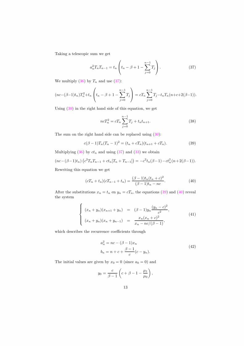
Taking a telescopic sum we get
a2nTnTn−1 = tn
tn − β + 1 −n−1∑
j=0
Tj
. (37)
We multiply (36) by Tn and use (37):
(nc−(β−1)tn)T 2n+tn
tn − β + 1 −n−1∑
j=0
Tj
= cTn
n−1∑
j=0
Tj−tnTn(n+c+2(β−1)).
Using (30) in the right hand side of this equation, we get
ncT 2n = cTn
n−1∑
j=0
Tj + tntn+1. (38)
The sum on the right hand side can be replaced using (30):
c(β − 1)Tn(Tn − 1)2 = (tn + cTn)(tn+1 + cTn). (39)
Multiplying (36) by ctn and using (37) and (33) we obtain
(nc−(β−1)tn)(
c2TnTn−1 + ctn[Tn + Tn−1])
= −c2tn(β−1)−ct2n(n+2(β−1)).
Rewriting this equation we get
(cTn + tn)(cTn−1 + tn) =(β − 1)tn(tn + c)2
(β − 1)tn − nc. (40)
After the substitutions xn = tn en yn = cTn, the equations (39) and (40) revealthe system
(xn + yn)(xn+1 + yn) = (β − 1)yn(yn − c)2
c2,
(xn + yn)(xn + yn−1) =xn(xn + c)2
xn − nc/(β − 1),
(41)
which describes the recurrence coefficients through
a2n = nc − (β − 1)xn
bn = n + c +β − 1
c(c − yn).
(42)
The initial values are given by x0 = 0 (since a0 = 0) and
y0 =c
β − 1
(
c + β − 1 − µ1
µ0
)
,
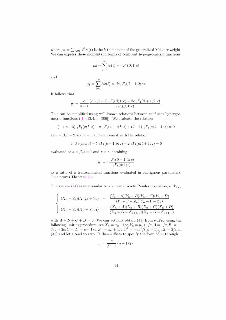
13
where µk =∑
`∈N0`kw(`) is the k-th moment of the generalized Meixner weight.
We can express these moments in terms of confluent hypergeometric functions
µ0 =
∞∑
`=0
w(`) = 1F1(β; 1; c)
and
µ1 =
∞∑
`=1
`w(`) = βc 1F1(β + 1; 2; c).
It follows that
y0 =c
β − 1
(c + β − 1) 1F1(β; 1; c) − βc 1F1(β + 1; 2; c)
1F1(β; 1; c).
This can be simplified using well-known relations between confluent hypergeo-metric functions ([1, §13.4, p. 506]). We evaluate the relation
(1 + a − b) 1F1(a; b; z)− a 1F1(a + 1; b; z) + (b − 1) 1F1(a; b− 1; z) = 0
at a = β, b = 2 and z = c and combine it with the relation
b 1F1(a; b; z)− b 1F1(a − 1; b; z)− z 1F1(a; b + 1; z) = 0
evaluated at a = β, b = 1 and z = c, obtaining
y0 = c1F1(β − 1; 1; c)
1F1(β; 1; c)
as a ratio of a transcendental functions evaluated in contiguous parameters.This proves Theorem 1.1.
The system (41) is very similar to a known discrete Painleve equation, αdPIV,
(Xn + Yn)(Xn+1 + Yn) =(Yn − A)(Yn − B)(Yn − C)(Yn − D)
(Yn + Γ − Zn)(Yn − Γ − Zn)
(Xn + Yn)(Xn + Yn−1) =(Xn + A)(Xn + B)(Xn + C)(Xn + D)
(Xn + ∆ − Zn+1/2)(Xn − ∆ − Zn+1/2)
with A + B + C + D = 0. We can actually obtain (41) from αdPIV using thefollowing limiting procedure: set Xn = xn−1/ε, Yn = yn+1/ε, A = 1/ε, B = −3/ε − 2c, C = D = c + 1/ε, Zn = zn + 1/ε, Γ2 = −4c2/((β − 1)ε), ∆ = 2/ε in(41) and let ε tend to zero. It then suffices to specify the form of zn through
zn =c
β − 1(n − 1/2) .
14
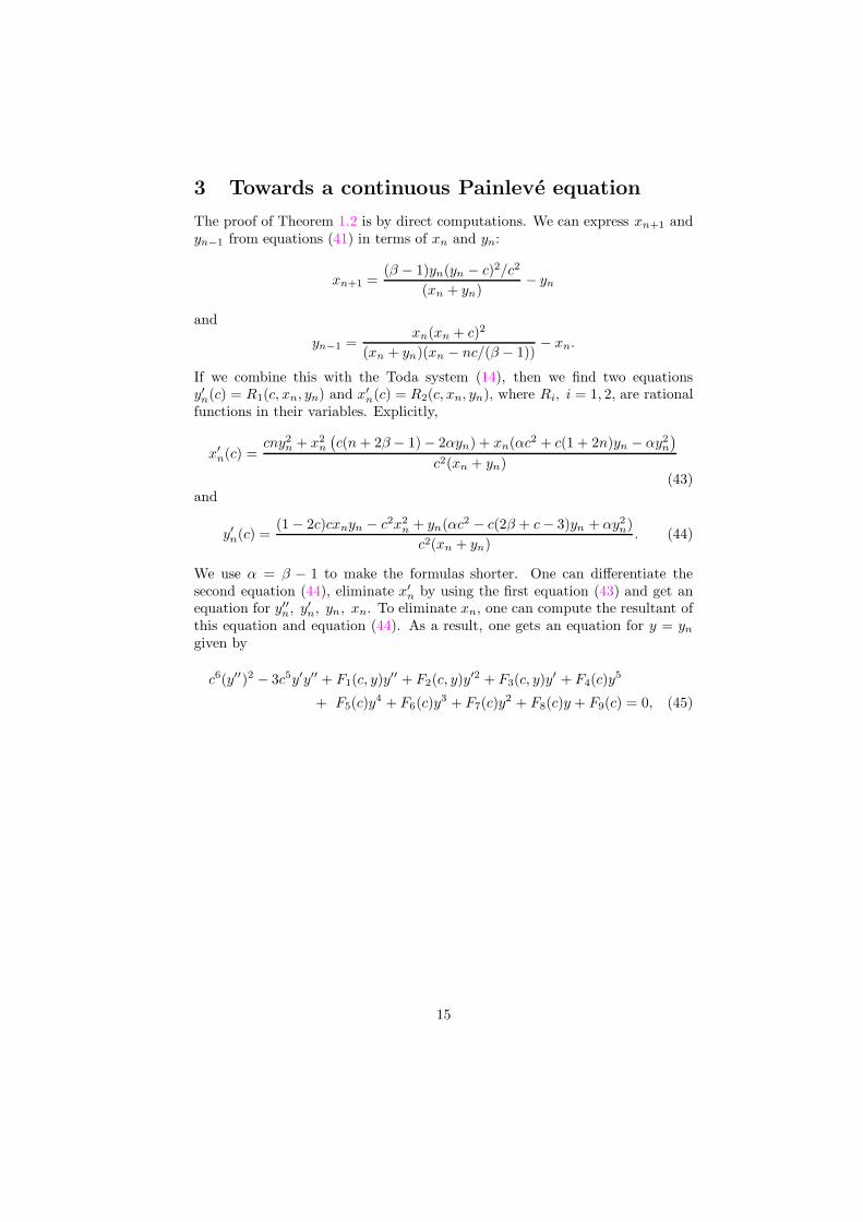
3 Towards a continuous Painleve equation
The proof of Theorem 1.2 is by direct computations. We can express xn+1 andyn−1 from equations (41) in terms of xn and yn:
xn+1 =(β − 1)yn(yn − c)2/c2
(xn + yn)− yn
and
yn−1 =xn(xn + c)2
(xn + yn)(xn − nc/(β − 1))− xn.
If we combine this with the Toda system (14), then we find two equationsy′n(c) = R1(c, xn, yn) and x′
n(c) = R2(c, xn, yn), where Ri, i = 1, 2, are rationalfunctions in their variables. Explicitly,
x′n(c) =
cny2n + x2
n
(
c(n + 2β − 1) − 2αyn) + xn(αc2 + c(1 + 2n)yn − αy2n
)
c2(xn + yn)(43)
and
y′n(c) =(1 − 2c)cxnyn − c2x2
n + yn(αc2 − c(2β + c − 3)yn + αy2n)
c2(xn + yn). (44)
We use α = β − 1 to make the formulas shorter. One can differentiate thesecond equation (44), eliminate x′
n by using the first equation (43) and get anequation for y′′n, y′n, yn, xn. To eliminate xn, one can compute the resultant ofthis equation and equation (44). As a result, one gets an equation for y = yn
given by
c6(y′′)2 − 3c5y′y′′ + F1(c, y)y′′ + F2(c, y)y′2 + F3(c, y)y′ + F4(c)y5
+ F5(c)y4 + F6(c)y
3 + F7(c)y2 + F8(c)y + F9(c) = 0, (45)
15
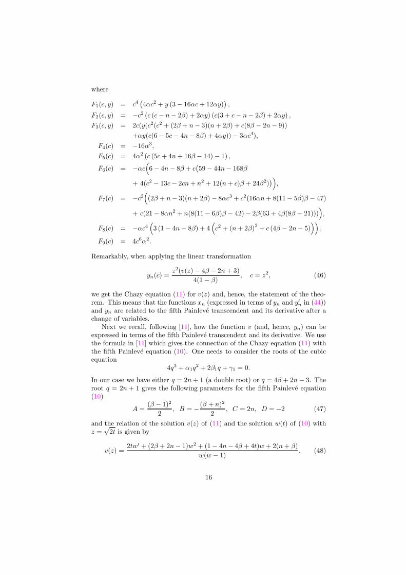
where
F1(c, y) = c4(
4αc2 + y (3 − 16αc + 12αy))
,
F2(c, y) = −c2 (c (c − n − 2β) + 2αy) (c(3 + c − n − 2β) + 2αy) ,
F3(c, y) = 2c(y(c2(c2 + (2β + n − 3)(n + 2β) + c(8β − 2n − 9))
+αy(c(6 − 5c − 4n− 8β) + 4αy)) − 3αc4),
F4(c) = −16α3,
F5(c) = 4α2 (c (5c + 4n + 16β − 14) − 1) ,
F6(c) = −αc(
6 − 4n − 8β + c(
59 − 44n− 168β
+ 4(c2 − 13c − 2cn + n2 + 12(n + c)β + 24β2))
)
,
F7(c) = −c2(
(2β + n − 3)(n + 2β) − 8αc3 + c2(16αn + 8(11− 5β)β − 47)
+ c(21 − 8αn2 + n(8(11− 6β)β − 42) − 2β(63 + 4β(8β − 21))))
,
F8(c) = −αc4(
3 (1 − 4n − 8β) + 4(
c2 + (n + 2β)2
+ c (4β − 2n− 5)))
,
F9(c) = 4c6α2.
Remarkably, when applying the linear transformation
yn(c) =z2(v(z) − 4β − 2n + 3)
4(1 − β), c = z2, (46)
we get the Chazy equation (11) for v(z) and, hence, the statement of the theo-rem. This means that the functions xn (expressed in terms of yn and y′n in (44))and yn are related to the fifth Painleve transcendent and its derivative after achange of variables.
Next we recall, following [11], how the function v (and, hence, yn) can beexpressed in terms of the fifth Painleve transcendent and its derivative. We usethe formula in [11] which gives the connection of the Chazy equation (11) withthe fifth Painleve equation (10). One needs to consider the roots of the cubicequation
4q3 + α1q2 + 2β1q + γ1 = 0.
In our case we have either q = 2n + 1 (a double root) or q = 4β + 2n − 3. Theroot q = 2n + 1 gives the following parameters for the fifth Painleve equation(10)
A =(β − 1)2
2, B = −(β + n)2
2, C = 2n, D = −2 (47)
and the relation of the solution v(z) of (11) and the solution w(t) of (10) withz =
√2t is given by
v(z) =2tw′ + (2β + 2n − 1)w2 + (1 − 4n − 4β + 4t)w + 2(n + β)
w(w − 1). (48)
16
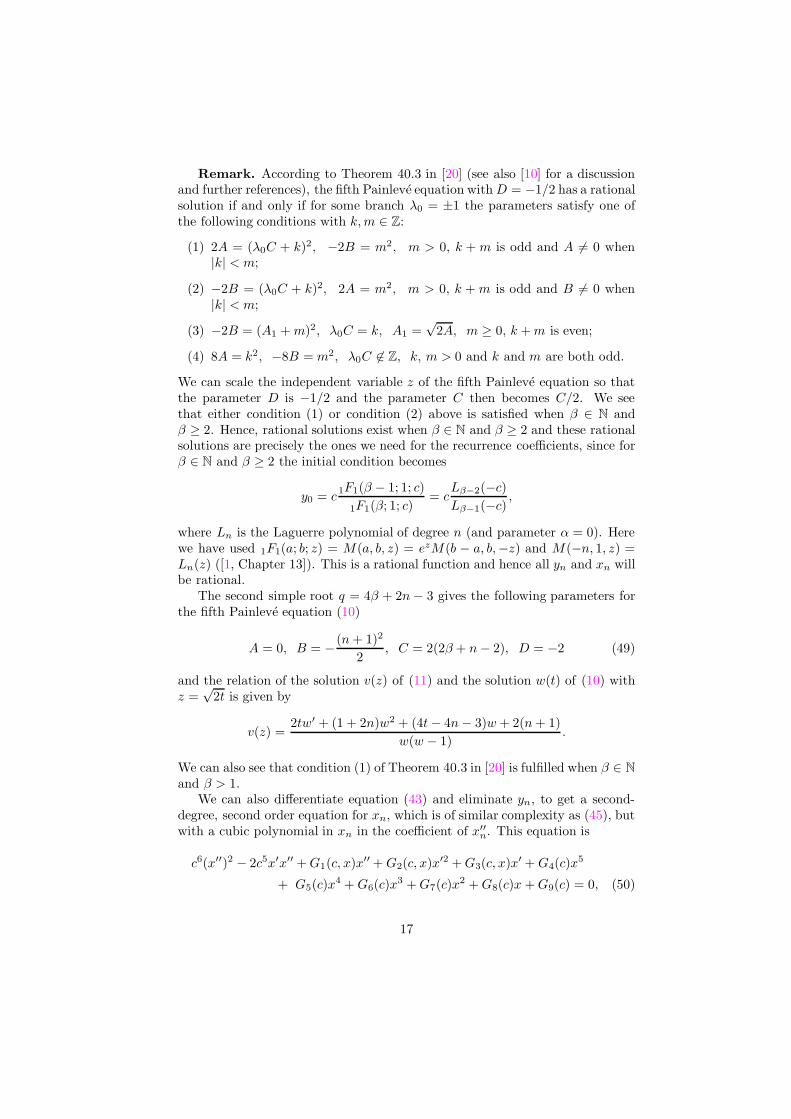
Remark. According to Theorem 40.3 in [20] (see also [10] for a discussionand further references), the fifth Painleve equation with D = −1/2 has a rationalsolution if and only if for some branch λ0 = ±1 the parameters satisfy one ofthe following conditions with k, m ∈ Z:
(1) 2A = (λ0C + k)2, −2B = m2, m > 0, k + m is odd and A 6= 0 when|k| < m;
(2) −2B = (λ0C + k)2, 2A = m2, m > 0, k + m is odd and B 6= 0 when|k| < m;
(3) −2B = (A1 + m)2, λ0C = k, A1 =√
2A, m ≥ 0, k + m is even;
(4) 8A = k2, −8B = m2, λ0C 6∈ Z, k, m > 0 and k and m are both odd.
We can scale the independent variable z of the fifth Painleve equation so thatthe parameter D is −1/2 and the parameter C then becomes C/2. We seethat either condition (1) or condition (2) above is satisfied when β ∈ N andβ ≥ 2. Hence, rational solutions exist when β ∈ N and β ≥ 2 and these rationalsolutions are precisely the ones we need for the recurrence coefficients, since forβ ∈ N and β ≥ 2 the initial condition becomes
y0 = c1F1(β − 1; 1; c)
1F1(β; 1; c)= c
Lβ−2(−c)
Lβ−1(−c),
where Ln is the Laguerre polynomial of degree n (and parameter α = 0). Herewe have used 1F1(a; b; z) = M(a, b, z) = ezM(b − a, b,−z) and M(−n, 1, z) =Ln(z) ([1, Chapter 13]). This is a rational function and hence all yn and xn willbe rational.
The second simple root q = 4β + 2n − 3 gives the following parameters forthe fifth Painleve equation (10)
A = 0, B = −(n + 1)2
2, C = 2(2β + n − 2), D = −2 (49)
and the relation of the solution v(z) of (11) and the solution w(t) of (10) withz =
√2t is given by
v(z) =2tw′ + (1 + 2n)w2 + (4t − 4n − 3)w + 2(n + 1)
w(w − 1).
We can also see that condition (1) of Theorem 40.3 in [20] is fulfilled when β ∈ N
and β > 1.We can also differentiate equation (43) and eliminate yn, to get a second-
degree, second order equation for xn, which is of similar complexity as (45), butwith a cubic polynomial in xn in the coefficient of x′′
n. This equation is
c6(x′′)2 − 2c5x′x′′ + G1(c, x)x′′ + G2(c, x)x′2 + G3(c, x)x′ + G4(c)x5
+ G5(c)x4 + G6(c)x
3 + G7(c)x2 + G8(c)x + G9(c) = 0, (50)
17
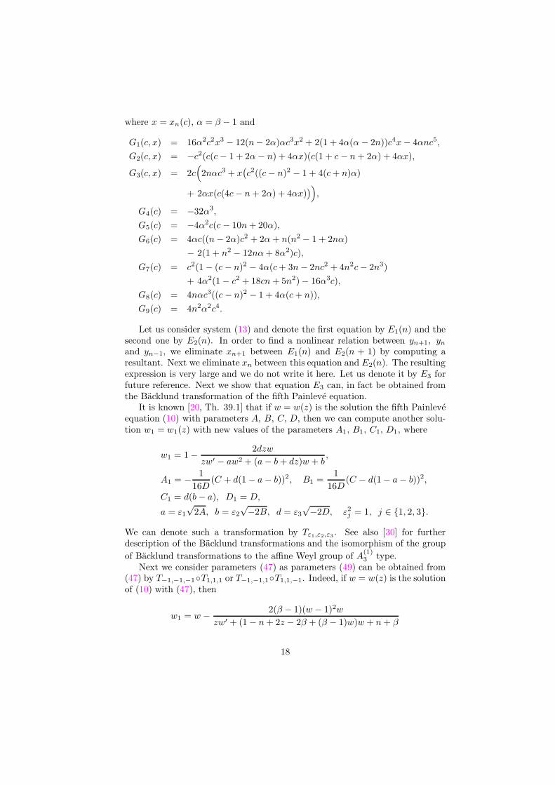
where x = xn(c), α = β − 1 and
G1(c, x) = 16α2c2x3 − 12(n− 2α)αc3x2 + 2(1 + 4α(α − 2n))c4x − 4αnc5,
G2(c, x) = −c2(c(c − 1 + 2α − n) + 4αx)(c(1 + c − n + 2α) + 4αx),
G3(c, x) = 2c(
2nαc3 + x(
c2((c − n)2 − 1 + 4(c + n)α)
+ 2αx(c(4c − n + 2α) + 4αx))
)
,
G4(c) = −32α3,
G5(c) = −4α2c(c − 10n + 20α),
G6(c) = 4αc((n − 2α)c2 + 2α + n(n2 − 1 + 2nα)
− 2(1 + n2 − 12nα + 8α2)c),
G7(c) = c2(1 − (c − n)2 − 4α(c + 3n − 2nc2 + 4n2c − 2n3)
+ 4α2(1 − c2 + 18cn + 5n2) − 16α3c),
G8(c) = 4nαc3((c − n)2 − 1 + 4α(c + n)),
G9(c) = 4n2α2c4.
Let us consider system (13) and denote the first equation by E1(n) and thesecond one by E2(n). In order to find a nonlinear relation between yn+1, yn
and yn−1, we eliminate xn+1 between E1(n) and E2(n + 1) by computing aresultant. Next we eliminate xn between this equation and E2(n). The resultingexpression is very large and we do not write it here. Let us denote it by E3 forfuture reference. Next we show that equation E3 can, in fact be obtained fromthe Backlund transformation of the fifth Painleve equation.
It is known [20, Th. 39.1] that if w = w(z) is the solution the fifth Painleveequation (10) with parameters A, B, C, D, then we can compute another solu-tion w1 = w1(z) with new values of the parameters A1, B1, C1, D1, where
w1 = 1 − 2dzw
zw′ − aw2 + (a − b + dz)w + b,
A1 = − 1
16D(C + d(1 − a − b))2, B1 =
1
16D(C − d(1− a − b))2,
C1 = d(b − a), D1 = D,
a = ε1
√2A, b = ε2
√−2B, d = ε3
√−2D, ε2
j = 1, j ∈ {1, 2, 3}.
We can denote such a transformation by Tε1,ε2,ε3. See also [30] for further
description of the Backlund transformations and the isomorphism of the group
of Backlund transformations to the affine Weyl group of A(1)3 type.
Next we consider parameters (47) as parameters (49) can be obtained from(47) by T−1,−1,−1◦T1,1,1 or T−1,−1,1◦T1,1,−1. Indeed, if w = w(z) is the solutionof (10) with (47), then
w1 = w − 2(β − 1)(w − 1)2w
zw′ + (1 − n + 2z − 2β + (β − 1)w)w + n + β
18
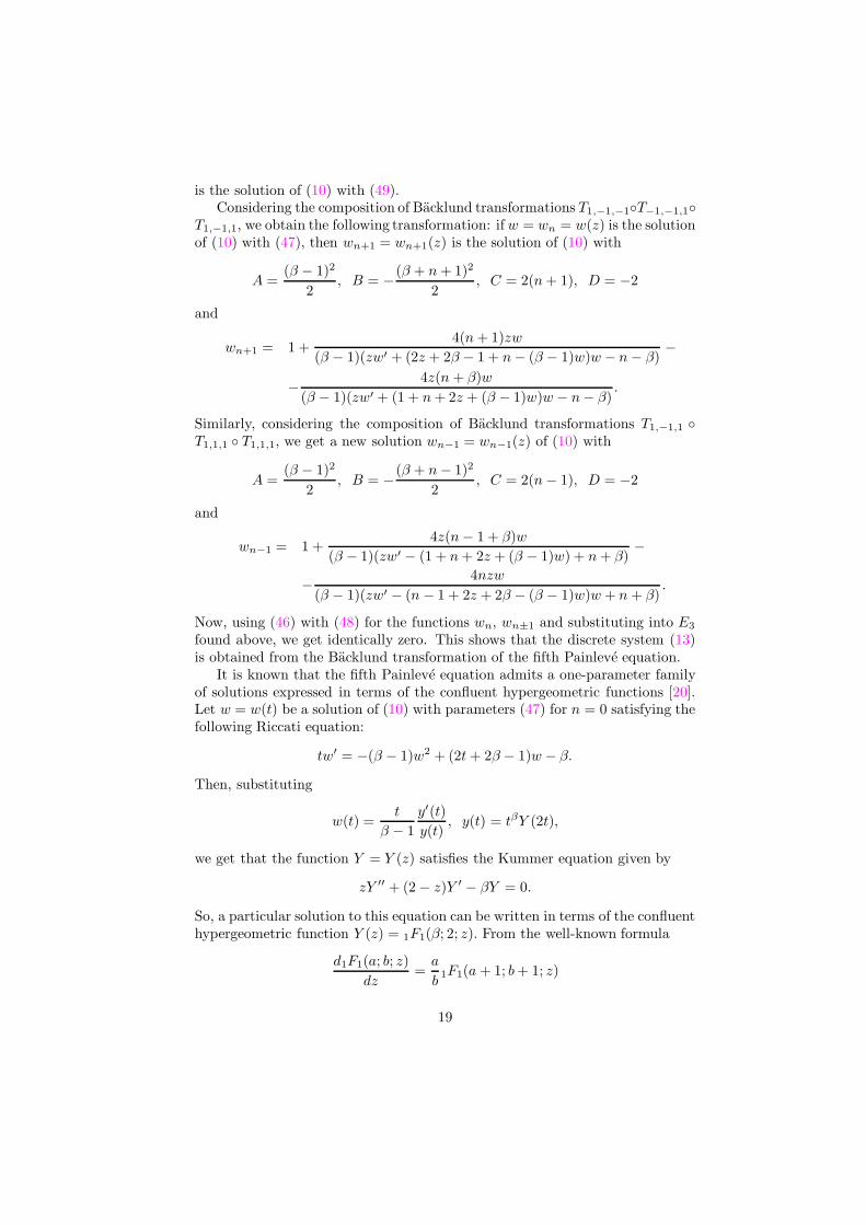
is the solution of (10) with (49).Considering the composition of Backlund transformations T1,−1,−1◦T−1,−1,1◦
T1,−1,1, we obtain the following transformation: if w = wn = w(z) is the solutionof (10) with (47), then wn+1 = wn+1(z) is the solution of (10) with
A =(β − 1)2
2, B = −(β + n + 1)2
2, C = 2(n + 1), D = −2
and
wn+1 = 1 +4(n + 1)zw
(β − 1)(zw′ + (2z + 2β − 1 + n − (β − 1)w)w − n − β)−
− 4z(n + β)w
(β − 1)(zw′ + (1 + n + 2z + (β − 1)w)w − n − β).
Similarly, considering the composition of Backlund transformations T1,−1,1 ◦T1,1,1 ◦ T1,1,1, we get a new solution wn−1 = wn−1(z) of (10) with
A =(β − 1)2
2, B = −(β + n − 1)2
2, C = 2(n − 1), D = −2
and
wn−1 = 1 +4z(n − 1 + β)w
(β − 1)(zw′ − (1 + n + 2z + (β − 1)w) + n + β)−
− 4nzw
(β − 1)(zw′ − (n − 1 + 2z + 2β − (β − 1)w)w + n + β).
Now, using (46) with (48) for the functions wn, wn±1 and substituting into E3
found above, we get identically zero. This shows that the discrete system (13)is obtained from the Backlund transformation of the fifth Painleve equation.
It is known that the fifth Painleve equation admits a one-parameter familyof solutions expressed in terms of the confluent hypergeometric functions [20].Let w = w(t) be a solution of (10) with parameters (47) for n = 0 satisfying thefollowing Riccati equation:
tw′ = −(β − 1)w2 + (2t + 2β − 1)w − β.
Then, substituting
w(t) =t
β − 1
y′(t)
y(t), y(t) = tβY (2t),
we get that the function Y = Y (z) satisfies the Kummer equation given by
zY ′′ + (2 − z)Y ′ − βY = 0.
So, a particular solution to this equation can be written in terms of the confluenthypergeometric function Y (z) = 1F1(β; 2; z). From the well-known formula
d1F1(a; b; z)
dz=
a
b1F1(a + 1; b + 1; z)
19
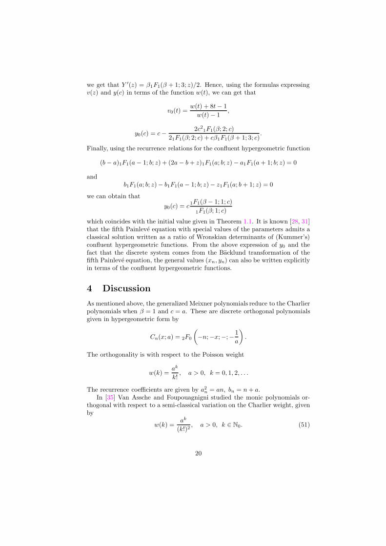
we get that Y ′(z) = β1F1(β + 1; 3; z)/2. Hence, using the formulas expressingv(z) and y(c) in terms of the function w(t), we can get that
v0(t) =w(t) + 8t − 1
w(t) − 1,
y0(c) = c − 2c21F1(β; 2; c)
21F1(β; 2; c) + cβ1F1(β + 1; 3; c).
Finally, using the recurrence relations for the confluent hypergeometric function
(b − a)1F1(a − 1; b; z) + (2a − b + z)1F1(a; b; z) − a1F1(a + 1; b; z) = 0
andb1F1(a; b; z)− b1F1(a − 1; b; z)− z1F1(a; b + 1; z) = 0
we can obtain that
y0(c) = c1F1(β − 1; 1; c)
1F1(β; 1; c)
which coincides with the initial value given in Theorem 1.1. It is known [28, 31]that the fifth Painleve equation with special values of the parameters admits aclassical solution written as a ratio of Wronskian determinants of (Kummer’s)confluent hypergeometric functions. From the above expression of y0 and thefact that the discrete system comes from the Backlund transformation of thefifth Painleve equation, the general values (xn, yn) can also be written explicitlyin terms of the confluent hypergeometric functions.
4 Discussion
As mentioned above, the generalized Meixner polynomials reduce to the Charlierpolynomials when β = 1 and c = a. These are discrete orthogonal polynomialsgiven in hypergeometric form by
Cn(x; a) = 2F0
(
−n;−x;−;−1
a
)
.
The orthogonality is with respect to the Poisson weight
w(k) =ak
k!, a > 0, k = 0, 1, 2, . . .
The recurrence coefficients are given by a2n = an, bn = n + a.
In [35] Van Assche and Foupouagnigni studied the monic polynomials or-thogonal with respect to a semi-classical variation on the Charlier weight, givenby
w(k) =ak
(k!)2, a > 0, k ∈ N0. (51)
20
These polynomials are generalized Charlier polynomials and satisfy a three-termrecurrence relation (5). The authors show that the recurrence coefficients canbe found as a (transformation of a) solution of dPII, with initial values in termsof the modified Bessel function
Iν(z) =
∞∑
k=0
1
k!
(z/2)2k+ν
Γ(k + ν + 1).
Namely,{
a2n = a
(
1 − x2n
)
,bn = n +
√axnxn+1,
where (xn)n satisfies the discrete Painleve II equation
xn−1 + xn+1 =nxn√
a (1 − x2n)
(52)
with initial values x0 = 1, x1 = I1(2√
a)/I0(2√
a). Moreover, the coefficientsa2
n(a) and bn(a) satisfy the Toda system (14) (with c replaced now by a). Us-ing the discrete equation (52) we can express xn+1 in terms of xn and xn−1.Substituting into the Toda system, we can express xn−1 in terms of xn and x′
n
xn−1(a) =nxn + 2ax′
n
2√
a(1 − x2n)
and substitute into the second equation of the Toda system. This results in thefollowing equation for the function x = xn(a):
x′′ =xx′2
x2 − 1− x′
a+
4a − n2 − 8ax2 + 4ax4
4a2(x2 − 1)x, (53)
where ′ = d/da. Applying a change of variables
xn(a) =w(z) + 1
w(z) − 1, a = z2
gives the fifth Painleve equation (10) for the function w(z) with parameters
A = −B =n2
8, C = 0, D = −8.
It is interesting to note that in [23, §8.3, p. 238] the fifth Painleve equation withparameters
A = −B =n2
8, C = 0, D = −2
appeared in relation to orthogonal polynomials on the unit circle. The initialconditions for (52) in [23] are x0 = 1 and x1 = −I1(λ)/I0(λ), so that λ = 2
√a,
which explains the difference in the coefficient D. Note that there is a misprinton [23, p. 238]: the minus sign in B is missing.
21
It can be easily seen that applying c = a/β, xn = xn/β in equation (50)and letting β tend to infinity, we get a differential equation for the function xn.Taking the change of variables
xn = a(x2 − 1)
we see that the function x(a) indeed satisfies equation (53). This is due tothe fact that the weights of the generalized Meixner polynomials tends to theweights of the generalized Charlier polynomials (51) in this limit.
Acknowledgments
We are grateful to the referees for their helpful comments and suggestions whichsubstantially improved the paper.
LB and WVA are supported by Belgian Interuniversity Attraction PoleP6/02, FWO grant G.0427.09 and K.U.Leuven Research Grant OT/08/033.Part of this work was carried out while GF was visiting K.U.Leuven for onemonth. The financial support of K.U.Leuven, MIMUW at the University ofWarsaw and the hospitality of the Analysis section at K.U.Leuven is gratefullyacknowledged. GF is also partially supported by Polish MNiSzW Grant N N201397937. Calculations were partially obtained in the Interdisciplinary Centre forMathematical and Computational Modelling (ICM), Warsaw University, withingrant G34-18. We would like to thank Arno Kuijlaars and Lun Zhang for theirhelpful comments and illuminating discussions.
References
[1] M. Abramowitz, I. Stegun, Handbook of Mathematical Functions, DoverPublications, New York, 1965.
[2] E. Basor and Y. Chen, Painleve V and the distribution function of a dis-
continuous linear statistic in the Laguerre unitary ensembles, J. Phys. A42 (2009), 035203, 18 pp.
[3] E. Basor, Estelle, Y. Chen and T. Ehrhardt, Painleve V and time-dependent
Jacobi polynomials, J. Phys. A 43 (2010), 015204, 25 pp.
[4] L. Boelen, Discrete Painleve Equations and Orthogonal Polynomials, Ph.D.thesis, K.U.Leuven, 2010.
[5] Y. Chen and M. V. Feigin, Painleve IV and degenerate Gaussian unitary
ensembles, J. Phys. A: Math. Gen. 39 (2006), 12381–12393.
[6] Y. Chen and A. Its, Painleve III and a singular linear statistics in Hermi-
tian random matrix ensembles, I, J. Approx. Theory 162 (2010), 270–297.
[7] Y. Chen and L. Zhang, Painleve VI and the unitary Jacobi ensembles,Preprint arXiv:0911.5636.
22

[8] Y. Chen and D. Dai, Painleve V and a Pollaczek-Jacobi type orthogonal
polynomials, Preprint arXiv:0809.3641.
[9] T. S. Chihara, An Introduction to Orthogonal Polynomials, Gordon andBreach, New York, 1978.
[10] P. A. Clarkson, Painleve equations—nonlinear special functions, LectureNotes in Mathematics 1883, Springer, Berlin, 2006, pp. 331–411.
[11] C. M. Cosgrove, Chazy’s second-degree Painleve equations, J. Phys. A:Math. Gen. 39 (2006), 11955–11971.
[12] A.S. Fokas, A.R. Its and A.V. Kitaev, Discrete Painleve equations and their
appearance in quantum gravity, Comm. Math. Phys. 142 (1991), 313–344.
[13] G. Freud, On the coefficients in the recursion formulae of orthogonal poly-
nomials, Proc. Roy. Irish Acad. Sect. A 76 (1976), 1–6.
[14] B. Gambier, Sur les equations differentielles du second ordre et du premier
degre dont l’integrale generale est a points critiques fixes, Acta Math. 33
(1910), 1–55.
[15] B. Grammaticos and A. Ramani, Discrete Painleve equations: coalescences,
limits and degeneracies, Physica A 228 (1996), 160–171.
[16] B. Grammaticos and A. Ramani, Discrete Painleve equations: a review,Lect. Notes Phys., 644, Springer, 2004, pp. 245–321.
[17] B. Grammaticos, A. Ramani and V. Papageorgiou, Do integrable mappings
have the Painleve property?, Phys. Rev. Lett. 67 (1991), 1825–1828.
[18] A. Ronveaux, Discrete semi-classical orthogonal polynomials: Generalized
Meixner, J. Approx. Theory 46 (1986), 403–407.
[19] A. Ronveaux, Asymptotics for recurrence coefficients of the generalized
Meixner case, J. Comput. Appl. Math. 133 (2001), 695–696.
[20] V.I. Gromak, I. Laine and S. Shimomura, Painleve Differential Equationsin the Complex Plane, Vol.28, Studies in Mathematics, de Gruyter, Berlin,NewYork, 2002.
[21] E. Hendriksen and H. van Rossum, Semi-classical orthogonal polynomials,in “Polynomes Orthogonaux et Applications”, Lecture Notes in Mathemat-ics 1171, Springer-Verlag, Berlin, 1985, pp. 354–361.
[22] W. Hahn, Uber die Jacobischen Polynome und zwei verwante Polynom-
klassen, Math. Zeit. 39 (1935), 634–638.
[23] M. E. H. Ismail, Classical and Quantum Orthogonal Polynomials in One
Variable, Encyclopedia of Mathematics and its Applications 98, CambridgeUniversity Press, 2005.
23

[24] M. E. H. Ismail, I. Nikonova and P. Simeonov, Difference equations and
discriminants for discrete orthogonal polynomials, Ramanujan J. 8 (2004),475–502.
[25] A.P. Magnus, Freud’s equations for orthogonal polynomials as discrete
Painleve equations, in Symmetries and Integrability of Difference Equations(Canterbury, 1996), London Math. Soc. Lecture Note Ser., 255, CambridgeUniversity Press, 1999, pp. 228–243.
[26] A.P. Magnus, Painleve-type differential equations for the recurrence coeffi-
cients of semi-classical orthogonal polynomials, J. Comp. Appl. Math. 57
(1995), 215–237.
[27] P. Maroni, Prolegomenes a l’etude des polynomes orthogonaux semi-
classiques, Ann. Mat. Pura Appl. (4) 149 (1987), 165–184.
[28] T. Masuda, Classical transcendental solutions of the Painleve equations and
their degeneration, Tohoku Math. J. 56 (2004), 457–490.
[29] J. Moser, Finitely many mass points on the line under the influence of an
exponential potential – an integrable system, Lecture Notes in Physics 38,Springer, Berlin, 1975, pp. 469–497.
[30] M. Noumi, Painleve equations through symmetry, Translations of Math-ematical Monographs, 223, American Mathematical Society, Providence,RI, 2004.
[31] K. Okamoto, Studies on the Painleve equations. II. Fifth Painleve equation
PV, Japan. J. Math. (N.S.) 13 (1987), 47–76.
[32] P. Painleve, Memoire sur les equations differentielles dont l’integrale
generale est uniforme, Bull. Soc. Math. Phys. France 28 (1900), 201–261.
[33] P. Painleve, Sur les equations differentielles du second ordre et d’ordre
superieure dont l’integrale generale est uniforme, Acta Math. 21 (1902),1–85.
[34] W. Van Assche, Discrete Painleve equations for recurrence coefficients of
orthogonal polynomials, in ”Difference Equations, Special Functions andOrthogonal Polynomials” (S. Elaydi et al., eds.), World Scientific, 2007,pp. 687–725.
[35] W. Van Assche and M. Foupouagnigni, Analysis of non-linear recurrence
relations for the recurrence coefficients of generalized Charlier polynomials,J. Nonlinear Math. Phys. 10 Supplement 2 (2003), 231–237.
Lies Boelen
Department of Mathematics
Katholieke Universiteit Leuven
Celestijnenlaan 200B box 2400
24
BE-3001 Leuven
Belgium
Galina Filipuk
Faculty of Mathematics, Informatics and Mechanics
University of Warsaw
Banacha 2
02-097 Warsaw
Poland
Walter Van Assche
Department of Mathematics
Katholieke Universiteit Leuven
Celestijnenlaan 200B box 2400
BE-3001 Leuven
Belgium
25