Human Capital and Convergence in a Non-Scale R&D

Growth Model∗

Chris PapageorgiouDepartment of EconomicsLouisiana State UniversityBaton Rouge, LA 70803

cpapa@lsu.edu

Fidel Perez-SebastianDpto. F. del Analisis Economico

Universidad de Alicante03071 Alicante, Spainfidel@merlin.fae.ua.es

May 2002

Abstract

This paper extends an R&D non-scale growth model to include endogenous human capital.The goal is to study the model predictions once the complementarity between technology andhuman capital commonly found in the empirical literature is taken into account. To do this, ahuman capital accumulation technology is proposed that preserves the non-scale nature of themodel. Our model suggests that cross-sector labor movements induced by the complementaritybetween human capital and technology can be a key factor in replicating and explaining growthmiracles such as Japan and South Korea. It is shown that the speed of convergence and theadjustment paths of output growth, investment rates, interest rates, and labor shares implied bythe proposed model are consistent with empirical evidence. Finally, it is argued that focusingonly on the asymptotic speed of convergence may not be very informative about the overallperformance of a model to explain the convergence phenomenon.

JEL Classification: O33, O41, O47.

Key words: Growth, R&D, human capital, input complementarity, cross-sector labor movement

∗We thank Craig Burnside, John Duffy, Jordi Caballe, Theo Eicher, Lutz Hendricks, Pete Klenow, Kazuo Mino,Pietro Peretto, Tomoya Sakagami, Chang Yonsung, John Williams, and seminar participants in many universitiesand conferences for their comments and suggestions. All remaining errors are our own.

1 Introduction

Surprisingly, there have been few attempts in the theoretical literature to explore growth models

with endogenous human capital and technical progress. In light of surging evidence that these two

engines are indeed complementary, it is the argument of this paper that they ought to be incor-

porated and studied within a unified growth model.1 As such, this paper extends Jones’ (1995)

hybrid R&D-based framework — admittedly one of various candidates — to include a formal schooling

sector.2 In particular, we present a model in which technical progress is enhanced through innova-

tion and imitation, and human capital through formal schooling. Even though formal schooling is

not the only source of human capital, we choose a schooling-based human capital technology be-

cause the model will ultimately be taken to the data following the approach suggested by Klenow

and Rodriguez-Clare (1997). Our choice of schooling technology is based on the Mincerian approach

(Mincer (1974)) that has recently been revived by Bils and Klenow (2000).3

The paper evaluates the model in three dimensions. First, we study its performance at steady-

state. By construction the steady-state properties of the model are consistent with Jones (1995).

Second, we obtain the asymptotic speed of convergence predicted by the model. We find that the

speed of convergence of output per worker is consistent with the evidence. However, it is shown

that this result alone may not be very informative about the overall performance of the model for

reproducing convergence episodes. In particular, we show that small variations in the asymptotic

speed of convergence implied by different models can produce substantial changes in the initial

periods of the adjustment path. This implies that models delivering empirically-supported speeds

of convergence may perform poorly at matching the whole convergence path. It is also shown that

the introduction of human capital makes the asymptotic speed of convergence much less sensitive

to external shocks such as policy actions. This finding gives theoretical support to Barro and Sala-

i-Martin’s (1995) result that convergence speed estimates do not vary substantially across different

countries or regions. However, this result can not be interpreted as necessarily implying that policy

1For a review of empirical studies supporting that human capital is complementary to technology innovation andimitation see Nelson and Pack (1999), Bils and Klenow (2000), and Caselli and Coleman (2001), just to name a few.

2Our choice of Jones (1995) as the benchmark in our investigation was based on the fact that the model succeededin reconciling important regularities in the data such as the increasing R&D intensity with constant output growthrates. Admittedly, a number of recent non-scale R&D growth models could be extended to include a schooling sector.These include Segerstrom (1998), Eicher and Turnovsky (1999a), Young (1998), Dinopoulos and Thompson (1998),and Howitt (1999). The last three papers also permit sustained output growth in the absence of population growth.

3For recent discussions on the advantages of the Mincerian approach in growth modeling and estimation, see Bilsand Klenow (2000), and Krueger and Lindahl (2001). Other papers that employ the Mincerian approach to modelschooling include Jones (1997, 2001), Jovanovic and Rob (1999), and Hall and Jones (1999). For an alternativemethod used to produce a human capital index, see Mulligan and Sala-i-Martin (2000).

1

actions have a negligible impact on the convergence speed because non-scale growth frameworks

deliver a time-varying speed of convergence.

Third, we examine the capacity of the model dynamics to reproduce fast output-convergence

episodes such as those of Japan and South Korea. Using standard technologies and parameteri-

zation, we show that our calibrated model is fairly successful in replicating rapid growth paths,

including the hump-shaped output growth adjustment paths associated with these experiences. It

is also found that the model can generate adjustment paths for interest and investment rates that

follow the patterns in the data. This is in sharp contrast to the counterfactual implications of the

standard one-sector neoclassical growth framework pointed out by King and Rebelo (1993). A key

factor contributing to these results is the complementarity between human capital and technology

adoption, which induces reallocation of labor across sectors along the adjustment path.

The implications of the Jones hybrid growth model have been extensively explored by Eicher

and Turnovsky (1999a, 1999b, 2001), and Perez-Sebastian (2000). Unlike us, they do not consider

human capital. There is however a small but rapidly growing literature that investigates the

relationship between human capital accumulation and technological progress, and their combined

effect on economic growth. Eicher (1996) and Lloyd-Ellis and Roberts (2000) develop models in

which both human capital and technological innovation are endogenous, but they are only concerned

with steady-state predictions. Restuccia (2001) presents a dynamic general equilibrium model with

schooling and technology adoption. He focuses on how schooling and technology adoption may

be amplifying the effects of productivity/policy differences on income disparity. Like us, Keller

(1996) and Funke and Strulik (2000) study transitional dynamics in a model of human capital and

blueprints. However, they do not take the predictions of their models to the data.

The remainder of the paper is organized as follows. Section 2 presents the basic model and

examines its steady-state properties. Attention is focused on the schooling sector which is the main

innovation of the model. Section 3 presents the transitional dynamics analysis. This section obtains

the asymptotic speed of convergence and transition paths implied by our model and compares these

results to existing models in the literature. Section 4 concludes.

2 The Basic Model

This section presents an economic growth model with endogenous human capital and technical

progress. Our exposition is focused on aggregate technologies. The main reason is that the human

2

capital technology incorporated in this paper can not be easily derived from a decentralized setup

due to aggregation problems.4 Another important reason is that previous papers that have analyzed

the type of non-scale framework that we incorporate in this paper have focused on the central

planner’s solution.

We start by describing the model economy’s environment. We then set up and solve the central

planner’s problem. Finally, we derive and discuss the steady-state implications of the model.

2.1 Economic environment

The population in this economy consists of identical infinitely-lived agents, and grows exogenously

at rate n. Agents are involved in three types of activities: consumption-good production, R&D

effort, and human capital attainment.5 Each period, consumers are endowed with one unit of time

that is allocated between working and studying. We abstract from labor/leisure decisions and

assume that agents have preference only over consumption.

Assume that at period t, output (Yt) is produced using human capital (HY t) and physical capital

(Kt) according to the following aggregate Cobb-Douglass technology:

Yt = AξtH

1−αY t K

αt , 0 < α < 1 , ξ > 0; (1)

where At is the economy’s technology level, ξ is the technology-output elasticity, and α is the share

of capital.

The R&D technology incorporates the only link between economies in our model. Ideas created

anywhere in the world can be copied by local researchers at a cost that diminishes with the coun-

try’s technological gap. The economy’s technology level evolves according to the following motion

equation:

At+1 −At = µAφtH

λAt

µA∗tAt

¶ψ

− δAAt, φ < 1, 0 < λ ≤ 1, ψ ≥ 0, A∗t ≥ At; (2)

where δA represents the technology depreciation rate; HAt is the portion of human capital employed

in the R&D sector at time t; A∗t is the worldwide technology frontier that grows exogenously at

rate gA∗ ; µ is a technology parameter; φ weights the effect of the stock of existing technology on

4See footnote 3 for papers that have also used the Mincerian approach to human capital and footnote 9 for adiscussion on the aggregation problem of this approach.

5Schooling is assumed to be the only source of human capital attainment in this model. Allowing for other types ofhuman capital attainment such as learning-by-doing (i.e. see Stokey (1988) and Lucas (1993)) would be an interestingextension of the model and worthy of future research.

3

R&D productivity; and λ captures decreasing returns to R&D effort.6 R&D equation (2) is a

modification of Jones (1995, 2001) R&D equation to allow for a catch-up term,³A∗tAt

´ψ, where ψ is

a technology-gap parameter. The catch-up term captures the idea that the greater the technology

gap between a leader and a follower, the higher the potential of the follower to catch up through

imitation of existing technologies.7

The production function given by (1) and the R&D equation given by (2) reflect the comple-

mentarity between technology and human capital. We consider that a higher human capital level

allows workers to use ideas more efficiently, and speeds up technology acquisition. Agents increase

their human capital through formal education provided by a schooling sector. The human capital

technology is of particular interest in our model and deserves careful consideration. Since our aim

is to take the model to the data then our specification ought to map the available data on average

years of education to the stock of human capital. Using the Mincerian interpretation seems to de-

liver such a specification. This representation follows Bils and Klenow (2000), who suggest that the

Mincerian specification of human capital is the appropriate way to incorporate years of schooling

to the aggregate production function. Following their approach, aggregate human capital is given

by

Hjt = ef(St)Ljt , j ∈ {Y,A} , (3)

where Ljt is the total amount of labor allocated to sector j; and St is the average educational

attainment of labor in period t. The derivative f 0(S) represents the return to schooling estimated

in a Mincerian wage regression: an additional year of schooling raises a worker’s efficiency by

6A decentralized setup behind these aggregate equations is, for example, that of Romer (1990). We can think oftechnology as the mass of intermediate-good varieties, xit, used in production. Under this interpretation, the term

AξtK

αt in expression (1) is a reduced form for [

R At0xαγit di]

1/γ ; where γ > 0 is a complementarity parameter. The twoproduction technologies are equal in the symmetric equilibrium case in which xit = xt , Kt = Atxt, and ξ = 1/γ−α.In Romer (1990), R&D effort results in new designs for use in new types of producer durables. There are incentives tocarry out R&D because when a new design is produced, an intermediate-good producer acquires a perpetual patentover the design. This allows the firm to manufacture the new variety and practice monopoly pricing.

7Nelson and Phelps (1966) are the first to construct a formal model based on the catch-up term. Parente andPrescott (1994) notice that this formulation implies that development rates increase over time (with A∗t ), and provideempirical evidence that is consistent with this implication. Coe and Helpman (1995), and Coe, Helpman, andHoffmaister (1997), among others, find evidence supporting the role of foreign-technology adoption in economicgrowth.

4

f 0(S).8,9

Next, we are concerned with the behavior of St. Suppose that at each date agents allocate time

to schooling only after supplying labor services to firms. Lt denotes the population size and LHt

the total amount of time allocated to schooling in period t. Assume that at the beginning of period

1 the average educational attainment equals zero. This implies that at the beginning of period 2,

S2 =LH1L1. Next period, given that consumers live for ever, the average years of schooling will be

S3 =LH1+LH2

L2, and so on. Hence, the average educational attainment can be written as

St =

Pt−1j=1 LHj

Lt. (4)

From equation (4), we can derive the law of motion of the average educational attainment as follows:

St+1 =StLt + LHtLt+1

. (5)

which in turn implies

St+1 − St =µ

1

1 + n

¶µLHtLt− nSt

¶. (6)

The evolution of S across time depends on the share of people in education LHL and the growth

rate of population, with the latter inducing a dilution effect.

2.2 Central planner’s problem

As we have mentioned previously, we focus on a centrally planned economy. A central planner

chooses the sequence {Ct, St, At, Kt, LY t, LAt, LHt}∞t=0 so as to maximize the lifetime utility of8Mincer (1974) estimates the following wage regression equation:

ωi = β0 + β1(SCH)i + β2(EXP )i + β3(EXP )2i + εi,

where ωi is the log wage for individual i, SCH is the number of years in school, EXP is the number of years of workexperience, and ε is a random disturbance term. Based on this micro-Mincer regression, Bils and Klenow (2000)present a more extensive formulation of expression (3) that includes schooling quality, and work experience.

9To be fully consistent with the Mincerian interpretation, Hjt =PLjt

i=1ef(sit); where sit is the educational at-

tainment of worker i at date t. The mapping between this expression and equation (3) is not straightforward, andhas not been addressed by the literature, with the exception of Lloyd-Ellis and Roberts (2000) who perform onlybalanced-growth path analysis in a finitely-lived agent framework. The difficulty arises because different cohorts canpossess different schooling levels. To make both expressions consistent, we could assume that the first generation ofagents pins down the workers’ educational attainment, and that posterior cohorts are forced to stay in school untilthey accumulate this educational level. In this way, all workers would have the same years of education (i.e., sit = Stfor all i) and then

PLjti=1

ef(sit) = Ljt ef(St). However, introducing these microfoundations into the model would

require to keep track of the different cohorts’ years of education across time, thus making the transitional dynamicsanalysis much more cumbersome, if not impossible. We leave this important issue to future research.

5

the representative consumer subject to the feasibility constraints of the economy, and the initial

values L0, S0,K0, and A0. The problem is characterized by the following set of equations:

max{Ct,St,At,Kt,LY t,LAt,LHt}

∞Xt=0

ρt

³CtLt

´1−θ − 11− θ

, (7)

subject to,

Yt = Aξt

hef(St)LY t

i1−αKαt , (8)

It = Kt+1 − (1− δK)Kt = Yt −Ct, (9)

At+1 −At = µAφt

hef(St)LAt

iλ µA∗tAt

¶ψ

− δAAt, (10)

St+1 − St =µ

1

1 + n

¶µLHtLt− nSt

¶, (11)

Lt = LY t + LAt + LHt, (12)

Lt+1Lt

= 1 + n, for all t, (13)

A∗t+1A∗t

= 1 + gA∗ , (14)

L0, S0, K0, A0 given,

where θ is the inverse of the intertemporal elasticity of substitution; and ρ is the discount factor.

Equation (9) is the economy’s feasibility constraint combined with the law of motion of the stock

of physical capital; it states that, at the aggregate level, domestic output must equal consumption,

Ct, plus physical capital investment, It. Equation (12) is the population constraint; labor force —

the number of people employed in the output and the R&D sectors — plus the number of individuals

in school must equal total population.

The optimal control problem can be stated as follows:

V (At,Kt, St) = max{LHt,LAt,It}

·Aξt [e

f(St)(Lt−LHt−LAt)]1−αKαt − It

Lt

¸1−θ− 1

1− θ+

+ρV

"At(1− δA) + µA

φt

³ef(St)LAt

´λµA∗tAt

¶ψ

;Kt(1− δK) + It ; St +1

1 + n

µLHtLt− nSt

¶#,(15)

where V (·) is a value function; LHt, LAt, It are the control variables; and At, Kt, St are thestate variables. Solving the optimal control problem obtains the Euler equations that characterize

6

the optimal allocation of population in human capital investment, in R&D investment, and in

consumption/physical capital investment as follows:µCtLt

¶−θ (1− α)YtLY t

=ρ

1 + n

µCt+1Lt+1

¶−θ (1− α)Yt+1LY,t+1

·1 + f 0(St+1)

µLY,t+1 + LA,t+1

Lt+1

¶¸, (16)

µCtLt

¶−θ (1− α)YtLY t

=ρ

1 + n

µCt+1Lt+1

¶−θ λ [At+1 − (1− δA)At]

LAt∗

∗ξYt+1At+1

+

·1− δA + (φ− ψ)

µAt+2 − (1− δA)At+1

At+1

¶¸ (1−α)Yt+1LY,t+1

λ(At+2−(1−δA)At+1)LA,t+1

, (17)µCtLt

¶−θ=

ρ

1 + n

µCt+1Lt+1

¶−θ ·αYt+1Kt+1

+ (1− δK)

¸. (18)

At the optimum, the central planner must be indifferent between investing one additional unit

of labor in schooling, R&D, and final output production. The LHS of equations (16) and (17)

represent the return from allocating an additional unit of labor to output production. The RHS

of equation (16) is the discounted marginal return to schooling, taking into account population

growth. The RHS term in brackets obtains because human capital determines the effectiveness of

labor employed in output production as well as in R&D. The RHS of equation (17) is the return to

R&D investment. An additional unit of R&D labor generates λ[At+1−(1−δA)]AtLAt

new ideas for new

types of producer durables. Every new design increases next period’s output by ξYt+1At+1

and R&D

production by dAt+2dAt+1

times (1−α)Yt+1LY,t+1

hλ(At+2−(1−δA)At+1)

LA,t+1

i−1; where (1−α)Yt+1LY,t+1

hλ(At+2−(1−δA)At+1)

LA,t+1

i−1denotes the value of an additional design that equalizes labor wages across sectors. Euler equation

(18) states that the planner is indifferent between consuming one additional unit of output today

and converting it into capital, thus consuming the proceeds tomorrow.

2.3 Steady-state growth

We next derive the model’s balanced-growth path. Solving for the interior solution, equation (12)

implies that in order for labor allocations to grow at constant rates, LHt, LY t and LAt must all

increase at the same rate as Lt. This means that the ratioLHtLt

is invariant along the balanced-

growth path. Hence, equation (11) implies that, at steady-state (ss), Sss is constant and equal

to

Sss =uH,ssn, (19)

where uH,ss =LHL

¯ss. Equation (19) shows that along the balanced growth path, the economy

invests in human capital just to provide new generations with the steady-state level of schooling.

7

Figure 1: Relationship between GA,ss and GA∗,ss

GA

GA*

GA < GA*GA > GA*

45o

GA = GA*

This is consistent with Jones (1997), where growth regressions are developed from steady-state

predictions; data on Sss acts as a proxy for uH,ss and the estimated coefficient on Sss partly reflects

the parameter 1n in our framework.

The aggregate production function, given by equation (8), combined with the steady-state

condition gY,ss = gK,ss delivers the gross growth rate of output as a function of the gross growth

rate of technology as

GY,ss = (GA,ss)ξ

1−α (1 + n) , (20)

where Gxt = 1 + gxt. Since GA,ss is constant, it follows from equation (2) that

GA,ss =h(1 + n)λGψ

A∗,ss

i 11+ψ−φ . (21)

Equation (21) presents the relationship between the technology growth rate of the model economy

and the technology frontier growth rate. This relationship is illustrated in Figure 1. Notice that

since the ratio ψ1+ψ−φ < 1, the function is concave with a unique point at which

GA,ss = GA∗,ss = (1 + n)λ

1−φ . (22)

GA,ss cannot be larger than GA∗,ss otherwise At will eventually become bigger than A∗t , and

this has been ruled out by assumption. But GA,ss can be smaller than GA∗,ss. For simplicity, we

focus on the special case in which all countries grow at the same rate at steady state; that is, we

8

assume that GA∗,ss is given by expression (22) and so is GA,ss.10 This in turn implies that

GY,ss = GC,ss = GK,ss = (1 + n)λξ

(1−α)(1−φ) . (23)

Consistent with Jones (1995) our balanced-growth path is free of “scale effects”, and policy has no

effect on long-run growth. The reason why our model’s long-run growth is equivalent to that of

Jones even in the presence of a schooling sector, is that at steady state the mean years of education,

St, reaches a constant level Sss.

2.4 Population shares in output, R&D, and schooling

Next, we derive the steady-state shares of labor in the three sectors of the economy. Euler equation

(16) combined with the balanced-growth equation (23) gives

uH,ss = 1− 1

f 0(Sss)

"Gθ−1y,ss (1 + n)

ρ− 1

#, (24)

where uH,ss =LHL

¯ss. Expectedly, the steady-state share of students in total population (uH,ss) is

positively related to the returns to education (f 0(Sss)), and the preference parameters (ρ, 1/θ).

Euler equation (17) combined with balanced-growth condition (23) delivers the steady-state

labor share in R&D as

uA,ss =uY,ss³

1−αλξ(gA,ss+δA)

´ hGθ−1y,ss

³GA,ss

ρ

´− (φ− ψ)(gA,ss + δA)− (1− δA)

i . (25)

As expected, R&D effort increases with the elasticities of technological change (φ − ψ) and final

output (ξ) with respect to the current stock of knowledge. R&D investment also increases as the

degree of diminishing returns to R&D effort decreases (i.e, as λ increases). Dividing equation (12)

by L gives the labor share in the output sector

uY,ss = 1− uh,ss − uA,ss. (26)

Equations (24), (25) and (26) represent the three steady-state shares of labor.

10Alternatively, we could assume that a technological leader moves the world technology frontier according toequation (2) which now reduces to

A∗t+1 −A∗t = µA∗φt (h∗AtL∗At)

λ − δAA∗t .

Notice that for the leader imitation is not possible since at the frontierA∗tAt

= 1. In such case G∗A = 1 + g∗A =

(1 + n∗)λ

1−φ as in Jones (1995). Assuming that n = n∗, and substituting G∗A into equation (21) delivers equation(22). As discuss in footnote 11, had g∗A taken on any other value, the transitional dynamics numerical analysis wouldbecome much more tedious.

9

3 Transitional Dynamics

This section is concerned with the transitional dynamics of the model economy. First, we redefine

variables so that their values remain constant at steady state. Second, we analyze the asymptotic

stability of the balanced growth equilibrium, and the asymptotic speed of convergence. Finally, we

assess the capacity of the model to reproduce two distinct miraculous growth experiences: Japan

and South Korea.

One of the main goals of the paper is to try to understand how the predictions of non-scale

growth models change when human capital is introduced. For this reason, an important aspect of

this work is to compare the predictions of our R&D model with human capital to those delivered

by the hybrid non-scale R&D growth model without human capital.

3.1 The normalized system

We start by redefining variables so that they take constant values along the balanced-growth path.

The aggregate production function, equation (8), suggests that we normalize variables by the

term Aξ

1−αt Lt. We can then rewrite consumption, physical capital and output as ct =

Ct

Aξ

1−αt Lt

,

kt =Kt

Aξ

1−αt Lt

and yt =Yt

Aξ

1−αt Lt

, respectively. Using equation (16) gives

µct+1ct

¶θ µuY,t+1uY t

¶(GAt)

(θ−1)ξ1−α

µytyt+1

¶=

µρ

1 + n

¶£f 0(St+1) (uY,t+1 + uA,t+1) + 1

¤. (27)

¿From the R&D equation (2), we derive GAt as

GAt =At+1At

= 1− δA + υhef(St)uAt

iλT (1+ψ−φ), (28)

where T =A∗tAt; and υ = µ (A∗t )

φ−1Lλt , which is a constant.

11 From equation (17) we obtainµct+1ct

¶θ µ ytyt+1

¶µuY,t+1uY t

¶=

ρ (gAt + δA)

Gξ

1−α (θ−1)+1At

µuA,t+1uAt

¶∗

∗"µ

λξ

1− α

¶ÃuY,t+1uA,t+1

!+

Ã1− δA

(gA,t+1 + δA)

!+ (φ− ψ)

#. (29)

Finally, from equation (18) we obtain

1 + n

ρ

·µct+1ct

¶(GAt)

ξ1−α

¸θ= α

yt+1

kt+1+ (1− δK). (30)

11To show that υ is constant requires some algebra. Rewriting the equality in its gross growth form,υt+1υt

=

Gφ−1A∗t (1+ n)

λ, and given that GA∗t = GA,ss = (1+ n)λ

1−φ , it follows thatυt+1υt

= 1. Notice that if A∗t did not growaccording to equation (22), υ could not be constant, making the simulation exercise more tedious.

10

The system that determines the dynamic equilibrium normalized allocations is formed by the

conditions associated with three control and three state variables as follows:

Control Variables:

1. Euler equation for population share in schooling, uht: Eq. (27).

2. Euler equation for population share in R&D, uAt: Eq. (29).

3. Euler equation for normalized consumption, ct: Eq. (30).

Subject to the population constraint uY t = 1− uAt − uht.State Variables:

1. Law of motion of human capital, St: Eq. (6).

2. Law of motion of the technology gap, Tt:

Tt+1 = Tt

µGA∗tGAt

¶. (31)

3. Law of motion of normalized physical capital, kt:

(1 + n)kt+1 (GAt)ξ

1−α = (1− δK)kt + yt − ct, (32)

where GAt is given by expression (28), GA∗t = GA,ss for all t, and

yt = kαt

hefY (St) uY t

i1−α. (33)

3.2 Asymptotic speed of convergence

The literature on transitional dynamics has devoted considerable time and effort in analyzing the

asymptotic speed of convergence predicted by growth models — that is, the rate at which a country’s

output approaches its balanced growth path once the country is sufficiently close to its long-run

equilibrium. Ortigueira and Santos (1997) and Eicher and Turnovsky (1999b, 2000), among others,

suggest that a desirable property for growth models is to deliver asymptotic speeds around 2 percent

that is consistent with most cross-country empirical studies.12 In addition, this analysis is crucial

to establishing the asymptotic stability of the model’s long-run equilibrium.

To compute the asymptotic speed of convergence we first linearize the normalized system of

Euler and motion equations around the steady state, and express the resulting system as follows:

~xt+1 = H ~xt;

12For example, Barro and Sala-i-Martin (1995) report convergence speeds that vary from 0.4%—3% in Japan, 0.4%—6% in the U.S. and 0.7%—3.4% in Europe. Temple (1998) reports estimates for OECD nations between 1.5% and3.6%.

11

where ~x is the vector consisting of the state and control variables; and H is the matrix of first

derivatives (∂xi,t+1/∂xjt) ∀i, j evaluated at the steady state, with xi being the ith component ofvector ~x. In our case, the transpose of this vector is ~x0t = (ct, uAt, uHt, kt, Tt, St). Second, we

compute the eigenvalues associated with the matrix H. Convergence speed is obtained by the

largest eigenvalue (denoted as eigen) among those contained in the unit circle. In particular, the

asymptotic speed of convergence (denoted as asc) of normalized variable y can be written as

asc(y) = −(yt+1 − yt)− (yt+1,ss − yt,ss)yt − yt,ss = 1− eigen.

Given that we are primarily interested in output per worker, YLA+LY

= yAξ

1−α (uA+uY )−1, we show

that its asymptotic speed of convergence equals

asc

µY

LA + LY

¶= (1− eigen)Gy,ss − gy,ss. (34)

To highlight the changes brought by the introduction of human capital into the model, we first

present results for a benchmark economy in which the schooling sector is closed. This corresponds

to the type of two-sector non-scale growth model studied, for example, by Eicher and Turnovsky

(1999a) and Perez-Sebastian (2000). The model is then characterized by two control variables

(consumption and R&D-labor) and two state variables (physical capital and technology gap), hence

~x0t = (ct, uAt, kt, Tt). It is straightforward to show that the system of equations that determine the

dynamics in this economy consists of Euler conditions (29) and (30), and motion equations (31) and

(32); subject to f(S) = 0, the population constraint uY t = 1− uAt, GA∗t = GA,ss, and equations(28) and (33). Eicher and Turnovsky (1999b, 2000) show that for relevant parameter values the

stable manifold is two dimensional. The adjustment path is then asymptotically stable and unique;

furthermore, growth rates and convergence speeds can, as a consequence, vary across time and

variables.

Closed-form solutions for matrix H do not exist and therefore we resort to numerical methods.13

We first choose parameter values (see table 1) for a benchmark economy that is very similar to

those considered by Eicher and Turnovsky (1999b, 2000). As such, our basic economy is without

a schooling sector and without imitation technology. There are only two sectors in this economy:

a final good sector that displays constant returns in labor and capital, but increasing returns

in knowledge; and an R&D sector that exhibits constant returns in knowledge and labor. Our

numerical methods obtain the asymptotic speed of convergence (asc(y)) to be equal to 0.0179 but

13All numerical results were obtained using MATHEMATICA. Programs are available by the authors upon request.

12

Table 1: Parameter values for the benchmark model with no human capital and no imitation

α 0.36 ξ 0.1 ρ 0.96 ψ 0

δK 0.06 λ 0.5 θ 1 Tss 1

δA 0.01 φ 0.5 n 0.015

the implied steady-state growth rate of output per worker (gy,ss) to be equal to 0.0023.14 On the

positive side, the model generates an asymptotic speed close to the 2 percent, consistent with most

empirical evidence. Indeed, this is the major finding of Eicher and Turnovsky (1999b, 2000) that

going from the neoclassical one-sector growth model to a two sector non-scale growth model reduces

the asymptotic speed of convergence from about 7 percent to more reasonable values.15 On the

negative side, the model generates output per capita growth rate equal to 0.23 percent which is

clearly inconsistent with evidence. For example, the average gy in Bils and Klenow’s (2000) 91-

country sample is 1.6 percent. Imposing the larger value of output growth (gy,ss = 0.016) requires

a substantially stronger increasing returns in the R&D sector (φ = 0.931) which in turn implies an

implausibly low asymptotic speed, asc(y) = −0.0042.16

Using the fact that asymptotic speed is positively related to the parameters λ, δA and ξ we

investigate whether admissible values for these parameters can deliver more reasonable results.

The parameter ξ = 0.1 is already at its upper bound of empirical estimates, but we can increase

the values of λ and δA to their upper bounds (λ = 0.75 and δA = 0.1).17 This exercise obtains

a reasonable value of asc(y) = 0.0156. An alternative and possibly more attractive solution to

obtaining reasonable values for both gy,ss and asc(y) is by introducing imitation in the model along

the lines of Parente and Prescott (1994) and Perez-Sebastian (2000). In our benchmark economy

when we assume φ = 0.931 (that results from imposing gy,ss = 0.016) and ψ = 0.16 (within the

calibrated values that we obtain in the following section), asc(y) becomes 0.0196 which is close to

14Notice that in the absence of a schooling sector output per worker equals output per capita.15These authors employ a continuous-time version of the model that provides slightly larger speeds than our discrete-

time approach. In particular, for the benchmark economy, the continuous-time analog would imply asc(y) = 0.0184.The slightly larger speed implied by continuous-time holds across all the models considered in our paper.16It is well known that the empirical literature does not offer much guidance about the value of φ. In our model,

this parameter is pinned down by the selected steady-state growth rate of the economy through equation (23), forgiven values of λ, n, ξ, and α.17Estimates of λ found in the literature vary from 0.2 (Kortum (1993)) to 0.75 (Jones and Williams (2000)).

Griliches (1988) reports estimates of the elasticity of output with respect to technology ξ between 0.06 and 0.1. If weconsider that δA includes the creative destruction effect of new technology on old designs, a value of 0.1 would implythat new ideas possess a life-span of 10 years, very close to the lower bound found by Caballero and Jaffe (1993).

13

Table 2: Parameter values for the proposed model with human capital and imitation

α 0.36 ξ 0.1 ρ 0.96 ψ 0.16 Tss 1

δK 0.06 λ 0.5 θ 1 η 0.69 Sss 12.03

δA 0.01 φ 0.931 n 0.015 β 0.43 gy,ss 0.016

most empirical estimates.

Next, we analyze the asymptotic speed of convergence in the model with schooling and imitation.

To do this, we need to calibrate the human capital technology. Following Bils and Klenow (2000),

we assume that

f(S) = ηSβ , η > 0, β > 0. (35)

Then using Psacharopoulos’ (1994) cross-country sample on average educational attainment and

Mincerian coefficients we estimate η and β. Given equation (35), we can construct the loglinear

regression equation

ln (Minceri) = a+ b lnSi + εi, (36)

where Minceri = f0(Si) is the estimated Mincerian coefficient for country i; a and b equal ln(ηβ)

and (β − 1) , respectively; and εi is a random disturbance term. We obtain estimates of η = 0.69

and β = 0.43, both significantly different from zero at the 1 percent level, that are very similar

to those obtained by Bils and Klenow (2000). Table 2 presents the parameter values used in our

numerical exercise. It includes the parameters used in the benchmark economy when we take

φ = 0.931 so as to impose gy,ss = 0.016, allow for imitation (ψ = 0.16) and the human capital

technology parameters (η = 0.69, β = 0.43). Given the above values, equations (19) and (24) imply

that the steady-state average educational attainment is 12.03 years, close to the 2000 U.S. figure

of 12.05 obtained by Barro and Lee (2000).

For the proposed model economy, the stable manifold is pinned down by three eigenvalues that

are contained within the unit circle. That is, the transition is characterized by a three-dimensional

stable saddle-path which in turn implies that the adjustment path is asymptotically stable and

unique.18

Our R&D model with human capital predicts an asymptotic speed of convergence for output

per worker equal to 0.0132. Note that even though this convergence speed is slightly lower than

18This result is robust to reasonable changes in the parameter values.

14

that of the model with no human capital and no imitation (asc(y) = 0.0179) or the model with no

human capital but with imitation (asc(y) = 0.0196), it is still well within empirical estimates. This

reduction in the convergence speed occurs because of the additional schooling sector present in our

model. A new sector implies that the same amount of available labor must now be allocated among

three (rather than two) sectors, and that state variables move slower towards the balanced-growth

path.

Another point worth noting here is that the asymptotic speed of convergence becomes much less

responsive to changes in parameter values when we introduce human capital (a new state variable)

in the model with imitation. For example, if δA increases from 0.01 to 0.1 our model with human

capital and imitation predicts a small increases in asc(y) from 0.0132 to 0.0172, whereas the model

with no human capital but with imitation predicts a very large increase from 0.0196 to 0.0410. In

addition, if λ increases from 0.5 to 0.75, then asc(y) increase from 0.0132 to 0.0145 in the former

model, and from 0.0196 to 0.0340 in the latter model. Finally, let us think about policy actions

that affect the technology-gap parameter ψ. This could occur, for example, because of changes

in the degree of barriers to technology adoption along the lines of Parente and Prescott (1994).

Suppose that a successful policy to enhance technological adoption causes ψ to increase from 0.16

to 0.25. Then our model with human capital predicts an asc(y) that increases from 0.0132 to 0.0168

whereas the model without human capital predicts an increase from 0.0196 to 0.0330. The reason

for the different response of the asymptotic speed in the two models is once again the additional

sector introduced in our model. That is, the presence of an additional sector into the model implies

a lower allocation of resources to each of the different sectors, thus reducing the impact of external

shocks.

This is consistent with Barro and Sala-i-Martin’s (1995) finding that estimated convergence

speeds do not vary much across different countries or regions. However, our result does not nec-

essarily imply that policy actions have a small impact on the convergence speed, as Barro and

Sala-i-Martin’s result has been interpreted. Far away from the balanced-growth path, policy may

have a larger effect on the speed of convergence over subsequent periods because the model allows

the convergence speed to vary across time. It is also important to notice that Barro and Sala-i-

Martin’s finding obtains for a fairly homogenous group of wealthy regions — namely, U.S. states,

European regions, and Japanese prefectures — which are probably close to their steady states.

In summary, we find that our non-scale R&D growth model with human capital obtains asymp-

totic speed of convergence consistent with the evidence. More importantly, our model’s implied

15

Table 3: Output, Capital and Schooling in Japan and S. Korea

Country 1960 1963 1990

JapanY per worker (%)∗∗

K per worker (%)∗∗

S (years)

20.616.910.2

60.3104.611.0∗

S. KoreaY per worker (%)∗∗

K per worker (%)∗∗

S (years)

11.011.63.2

42.250.27.7∗

∗ 1987 figures.∗∗ Levels relative to their U.S. counteparts.

asymptotic speed of convergence is much less responsive to policy actions compared to existing

models in the literature.

3.3 Adjustment paths of Japan and South Korea

At least since the seminal work of Lucas (1993), it has been recognized that a desirable property of

growth models is to be able to reproduce miraculous experiences. In terms of transitional dynamics

analysis, this amounts at least to being able to reproduce the average speed of convergence, and

country-specific changes in the output growth trend. In this section, we focus on the S. Korean

and the Japanese output paths because they represent two very distinct growth experiences. Table

3 presents data for S. Korea and Japan on relative GDP per worker, relative physical capital per

worker, and average educational attainment.19 Between 1960 and 1990, Japan’s relative output per

worker increased from 20.6 to 60.3 percent. GDP per worker in S. Korea started its fast growing

path around 1963; during the period 1963-1990, its relative level increased from 11.0 to 42.2 percent.

During these periods, Japan and S. Korea exhibited a 5.2 and 6.5 percent average annual growth

rates, respectively.

Japan had lost a substantial portion of its physical capital during WWII, but its educational

attainment in 1960 of 10.2 years compared well with those of the most developed nations — e.g., the

U.S. educational attainment at that time was a little over 10.7.20 What is even more interesting

is that during the period 1960-1987, average years of schooling per worker increased only by 0.8

19All relative measures in the paper are with respect to U.S. levels. Additionally, we follow Parente and Prescott(1994) and smooth all data series using the Hodrick-Prescott filter with the smoothing parameter equal to 25.20Human capital levels in Japan were high before WWII. After the Meiji Restoration of 1868, one of the policy

priorities of the Meiji government was to introduce a nationwide education system under which all children from 6through 13 years of age were required to attend school (see Ozawa 1985).

16

Figure 2: Adjustment paths for Japan and S. Korea

0

10

20

30

40

50

60

1950 1955 1960 1965 1970 1975 1980 1985 1990

Rel

ativ

e G

DPW

(%)

Japanese DataPredictions w/o HPredictions with H

0

10

20

30

40

50

60

1960 1965 1970 1975 1980 1985 1990

Rel

ativ

e G

DPW

(%)

Korean DataPredictions w/o HPredictions with H

0123456789

101112

1950 1955 1960 1965 1970 1975 1980 1985 1990

RG

DPW

gro

wth

(%)

Japanese Data

Predictions w/o H

Predictions with H

0123456789

101112

1960 1965 1970 1975 1980 1985 1990

RG

DPW

gro

wth

(%)

Korean Data

Predictions w/o H

Predictions with H

years to reach 11.0 years. The main engine of growth in Japan seems to have been physical capital

accumulation induced in part by a very important technological catch-up process.21 In 1960, the

Japanese physical capital stock per worker was only 16.9 percent; in 1990 reached a stunning 104.6

percent, which implies an average annual convergence rate of 6.3 percent.

The S. Korean growth experience is distinctly different from the Japanese experience. Even

though output convergence was faster in S. Korea, physical capital accumulation was lower than in

Japan, growing from 11.6 to 50.2 percent — an average annual convergence rate of 5.6 percent. As

shown in table 3, human capital accumulation played a much larger role in the development process

of S. Korea. In particular, the average educational attainment per worker more than doubled in

the period 1963-1987, increasing from 3.2 to 7.7 years.

In this section, we examine the ability of the proposed model to replicate these two nations’

convergence episodes by simulating its transitional dynamics. Because there is no analytical solu-

tion to our system of Euler and motion equations, we once again resort to numerical approximation

techniques. More specifically, we follow Judd (1992) to solve the dynamic equation system, approx-

21For discussion on the effects of technology adoption on East Asia see Amsden (1991) and Baark (1991). For anexcellent presentation of technology adoption in Japan see Minami (1994). The author explores three categories ofborrowed technology which are illustrated by examples from Japanese history. He discusses in detail the introductionof the English railway technology, the machine filature technology and the silk weaving technology. According toMinami, Japan’s industrialization was revolutionary in the sense that it was accomplished by the adoption of existingforeign technology.

17

imating the policy functions employing high-degree polynomials in the state variables.22

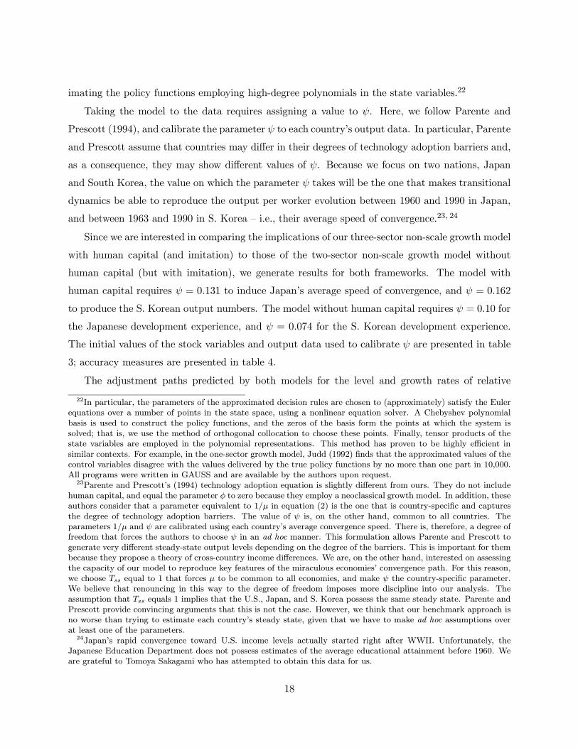
Taking the model to the data requires assigning a value to ψ. Here, we follow Parente and

Prescott (1994), and calibrate the parameter ψ to each country’s output data. In particular, Parente

and Prescott assume that countries may differ in their degrees of technology adoption barriers and,

as a consequence, they may show different values of ψ. Because we focus on two nations, Japan

and South Korea, the value on which the parameter ψ takes will be the one that makes transitional

dynamics be able to reproduce the output per worker evolution between 1960 and 1990 in Japan,

and between 1963 and 1990 in S. Korea — i.e., their average speed of convergence.23, 24

Since we are interested in comparing the implications of our three-sector non-scale growth model

with human capital (and imitation) to those of the two-sector non-scale growth model without

human capital (but with imitation), we generate results for both frameworks. The model with

human capital requires ψ = 0.131 to induce Japan’s average speed of convergence, and ψ = 0.162

to produce the S. Korean output numbers. The model without human capital requires ψ = 0.10 for

the Japanese development experience, and ψ = 0.074 for the S. Korean development experience.

The initial values of the stock variables and output data used to calibrate ψ are presented in table

3; accuracy measures are presented in table 4.

The adjustment paths predicted by both models for the level and growth rates of relative

22In particular, the parameters of the approximated decision rules are chosen to (approximately) satisfy the Eulerequations over a number of points in the state space, using a nonlinear equation solver. A Chebyshev polynomialbasis is used to construct the policy functions, and the zeros of the basis form the points at which the system issolved; that is, we use the method of orthogonal collocation to choose these points. Finally, tensor products of thestate variables are employed in the polynomial representations. This method has proven to be highly efficient insimilar contexts. For example, in the one-sector growth model, Judd (1992) finds that the approximated values of thecontrol variables disagree with the values delivered by the true policy functions by no more than one part in 10,000.All programs were written in GAUSS and are available by the authors upon request.23Parente and Prescott’s (1994) technology adoption equation is slightly different from ours. They do not include

human capital, and equal the parameter φ to zero because they employ a neoclassical growth model. In addition, theseauthors consider that a parameter equivalent to 1/µ in equation (2) is the one that is country-specific and capturesthe degree of technology adoption barriers. The value of ψ is, on the other hand, common to all countries. Theparameters 1/µ and ψ are calibrated using each country’s average convergence speed. There is, therefore, a degree offreedom that forces the authors to choose ψ in an ad hoc manner. This formulation allows Parente and Prescott togenerate very different steady-state output levels depending on the degree of the barriers. This is important for thembecause they propose a theory of cross-country income differences. We are, on the other hand, interested on assessingthe capacity of our model to reproduce key features of the miraculous economies’ convergence path. For this reason,we choose Tss equal to 1 that forces µ to be common to all economies, and make ψ the country-specific parameter.We believe that renouncing in this way to the degree of freedom imposes more discipline into our analysis. Theassumption that Tss equals 1 implies that the U.S., Japan, and S. Korea possess the same steady state. Parente andPrescott provide convincing arguments that this is not the case. However, we think that our benchmark approach isno worse than trying to estimate each country’s steady state, given that we have to make ad hoc assumptions overat least one of the parameters.24Japan’s rapid convergence toward U.S. income levels actually started right after WWII. Unfortunately, the

Japanese Education Department does not possess estimates of the average educational attainment before 1960. Weare grateful to Tomoya Sakagami who has attempted to obtain this data for us.

18

Table 4: Accuracy measures in different models

Average Error (%)∗ Max. Error (%)∗

Country Model ∗∗ ψ C uH uA C uH uAJapan model w/ H 0.131 0.01 0.02 0.01 0.04 0.07 0.04Japan model w/ h 0.132 0.01 0.02 0.01 0.04 0.07 0.04Japan model w/o H 0.10 0.00 −.− 0.00 0.01 −.− 0.02S. Korea model w/ H 0.162 0.06 0.17 0.06 0.27 0.78 0.24S. Korea model w/ h 0.14 0.06 0.17 0.06 0.27 0.73 0.23S. Korea model w/o H 0.074 0.01 −.− 0.01 0.02 −.− 0.05∗ We assess the Euler equation residuals over 10,000 state-space points using the approximated rules. Foreach variable, the measure gives the current value decision error that agents using the approximated

rules make, assuming that the (true) optimal decisions were made in the previous period. Santos (2000)

shows that the residuals are of the same order of magnitude as the policy function approximation error.∗∗ model w/ H refers to the three-sector non-scale growth model with schooling sector.

model w/o H refers to the two-sector non-scale growth model without schooling sector.

model w/ h refers to the three-sector growth non-scale model assuming that per worker variables are obtained by dividing by L.

GDP per worker (RGDPW) are depicted in figure 2. The predicted paths replicate fairly well the

Japanese and the S. Korean output paths. Our model with human capital, however, does a much

better job because it predicts that output per worker growth rates do not pick at the beginning of

the adjustment path but later on. This is an important feature that can not be either reproduced

by the standard one-sector neoclassical growth model (see King and Rebelo (1993)), and that

characterizes the output-convergence phenomenon as Easterly and Levine (1997), among others,

show.

3.4 Discussion of the transition results

What are the determining factors behind our results? We can write production function (8) in per

worker terms as follows:µYt

LY t + LAt

¶= Aξ

tef(St)(1−α)

µLY t

LY t + LAt

¶1−α µ KtLY t + LAt

¶α

. (37)

Using a continuous time approximation, equation (37) can be rewritten in its output per worker

growth (gwY ) form

gwY t = ξgAt + (1− α)d f(St)

d t+ αg(K/L),t +

h(1− α) guY ,t − g(1−uH),t

i. (38)

Equation (38) presents a decomposition of output growth in its four components: (a) growth of

total factor productivity (TFP), (b) change in per capita educational attainment, (c) growth of

19

per capita physical capital, (d) net impact of labor movements across sectors (term in squared

brackets). Given that the population size in our model evolves exogenously, this decomposition

captures the impact of the different aggregates that enter the production function including the

labor force size.

Figures 3 and 4 present the contributions of the four different components to the S. Korean

and the Japanese output per worker growth, according to equation (38). We present the growth

components for three different R&D models with imitation. A thin-black line represents predictions

of the two-sector non-scale growth model without human capital accumulation (denoted as the

model w/o H). Recall that in this model variables presented in their per capita or their per worker

intensive form are identical as there is no schooling sector which would attract some of the labor

force. As a result, the terms (1− α) d f(St)d t and g(1−uH),t in equation (38) equal zero. A thick-black

line, represents predictions for our model with human capital (denoted as the model w/ H); the

intensive form of all relevant variables are in per worker terms (dividing by LY + LA ). A dashed

line represents predictions of a non-scale growth model with human capital but with the additional

assumption that per worker variables come from dividing by L (the population size), instead of

by LY + LA (the labor force) (denoted as the model w/ h). As a result, the second summand

within the squared brackets in equation (38) vanishes. One of the determining features of this last

formulation of our proposed model is that it does not consider movements in and out the labor

force from and to the schooling sector. This model is examined in the hope that it will reveal which

effect of the complementarity between human capital and technology dominates; the one on TFP

that occurs though the R&D equation, or the one that takes place through labor movement among

sectors. Finally, a grey line depicts the data for each country.

We start our analysis with a few general points. Notice that if RGDPW growth rates obtain

large values early on, they must fall rapidly later on, and vice versa. This feature of the transitional

path of output growth is due to the fact that all of the models considered are calibrated to reproduce

the average convergence speed of RGDPW. Having this in mind, we can focus on model differences

that occur during the early periods of the adjustment path. Another feature common to all three

models is the initial values of the capital stocks from which the transition dynamics start. This

implies that initial incentives to invest in physical and human capital formation (when the model

includes a schooling sector) are very similar in the three cases, because by construction, so are

the initial capital-output ratios and average educational attainments. As a consequence, the main

forces behind the initial differences in RGDPW growth rates across models are the growth rate of

20

relative TFP and the net contribution of labor (see figures 3 and 4; panels B and E).

Let us now compare the dashed line (denoting themodel w/ h) and the thin-black line (denoting

themodel w/o H) in a attempt to understand the contribution of introducing human capital into the

model and abstracting from the effect of movements into and out the labor force. The introduction

of the new sector amplifies the effect of diminishing returns, increasing greatly initial growth rates.

The new schooling sector adds a new growth engine whose contribution to the growth rate at impact

lies around 4 percent for S. Korea and 0.33 percent for Japan (see panel D), and thereafter follows

the standard neoclassical declining-growth-rate pattern caused by diminishing returns.

Another important effect of introducing schooling is that the final-output labor share starts

further away from its steady state level and subsequently grows faster, thus making much larger its

initial contribution (see panel E). The reason is that schooling is the only activity that enhances

the productivity of the other two sectors, and consequently it is optimal for the economy to invest

heavily in human capital at the beginning of the adjustment path, borrowing resources mainly

from the consumption-good sector. Due to the same reason, physical capital suffers a slightly

larger initial fall in the model with schooling, and accumulates at a faster rate during the first

few periods following the evolution of output (see panel C). The big initial differences between the

growth rates of output and capital in both models are due to consumption smoothing, which pulls

down the investment share as output declines, causing physical capital to grow at a much lower

rate than output during the first few periods.

Continuing our comparison between the dashed line (model w/ h) to the thin-black line (model

w/o H) in figures 3 and 4 (panel B), we see that the relative TFP contribution is smaller in themodel

w/ h. This occurs because the shocks to physical capital and output are the same for both models,

but in the model w/ h schooling formation also enhances the output catch-up process. As a result,

the initial technology gap required by this model becomes smaller thus decreasing the productivity

of the R&D sector and the contribution of TFP due to the existence of diminishing imitation

opportunities. Note that R&D productivity declines so much that the technology-gap parameter ψ

must rise to allow the model to reproduce the Japanese and S. Korean average convergence speeds.

Panel B in figure 3 clearly illustrates that human capital speeds up technology adoption. The

contribution of TFP to output growth is presented by a hump-shaped pattern. This pattern, which

turns out to also describe the evolution of the R&D labor share, is the consequence of two opposing

effects. On the one hand, the technology imitation productivity declines with technology gap. On

the other hand, R&D becomes more productive as the average educational attainment grows. The

21

latter effect dominates the former during the first few periods, whereas the reverse is true later

on.25

Our investigation of the model w/o H and the model w/ h reveals that neither model can

replicate the hump-shaped output growth path evident in the data. We next compare the model

w/ h (per worker variables are obtained by dividing by the population size, L) with the model w/

H (per worker variables are obtained by dividing by the labor force size, LY + LA). The former

model is once again illustrated by the dashed lines whereas the latter model is illustrated by the

thick solid line.

Notice that the contribution of human capital is almost identical in both cases (see panel D).

The hump-shaped physical capital contribution illustrated by the two lines is also the same, and

complies well with the S. Korean data (see panel C). A strong and declining consumption smoothing

effect causes the initial increase; but after a few periods diminishing-returns dominate and physical

capital growth rates start to decrease, and continue doing so as they approach their steady-state

level. There is a distinct difference between the two models though: the model w/ H (depicted

by the thick-black line) shows a larger decrease in physical capital investment during the first two

periods, and a faster physical capital growth thereafter. This is the consequence of matching the

same initial data values to per worker variables, instead of per capita. Notice that at impact

physical capital and output must be further away from their balanced-growth path in the former

case, because the initial labor force is also below its steady-state value. The lower level of physical

capital at impact produces larger returns, and raises its subsequent growth rates. The lower initial

level of output along with the preference for consumption smoothing create the larger decrease in

physical capital investment during the first two periods. The contribution of relative TFP in the

model w/ H is stronger along the whole adjustment path (see panel B) because the slightly-larger

initial technical gap required in the per-worker-term case raises R&D productivity. The difference

is larger for S. Korea because the value of the parameter ψ required is also larger.

The main difference between the two models is due to the net labor contribution illustrated in

panel E. Recall that net labor contribution is given by the term in brackets in equation (38), and

reflects the effect of population movements across sectors. More specifically, this term takes into

account that output growth rises with the amount of labor devoted to final-good production, but

also that additional labor deflates output per worker. As a consequence, net labor contribution

25Lau and Wan (1933) suggest that the ability of human capital to enhance technology adoption may explain themiraculous experiences that achieve their maximum growth rates after trend acceleration. Our work shows that, atleast in our structural model w/ h, human capital and TFP can not explain the output growth inverted-U path inJapan and S. Korea.

22

Figure 3: Contribution of different components to relative output growth, S. Korea

-3

-2

-1

0

1

2

3

4

5

6

7

8

9

1964 1969 1974 1979 1984 1989

RG

DPW

gro

wth

(%)

Panel (A)

-3

-2

-1

0

1

2

3

4

5

6

7

8

9

1964 1969 1974 1979 1984 1989

RTF

P gr

owth

(%)

Panel (B)

-3

-2

-1

0

1

2

3

4

5

6

7

8

9

1964 1969 1974 1979 1984 1989

Rk

grow

th (%

)

Panel (C)

-3

-2

-1

0

1

2

3

4

5

6

7

8

9

1964 1969 1974 1979 1984 1989

Rh

grow

th (%

)

Panel (D)

-3

-2

-1

0

1

2

3

4

5

6

7

8

9

1964 1969 1974 1979 1984 1989

Net

labo

r con

trib

utio

n (%

)

Panel (E)

Variables: RGDPW is relative GDP per worker; Rk is relative physical capital per capita; Rh is relative human

capital per capita; Net labor contribution represents the effect of the terms in brackets in equation (38).

23

Figure 4: Contribution of different components to relative output growth, Japan

-3

-2

-1

0

1

2

3

4

5

6

7

8

9

1961 1966 1971 1976 1981 1986

RG

DPW

gro

wth

(%)

Panel (A)

-3

-2

-1

0

1

2

3

4

5

6

7

8

9

1961 1966 1971 1976 1981 1986

RTF

P gr

owth

(%)

Panel (B)

-3

-2

-1

0

1

2

3

4

5

6

7

8

9

1961 1966 1971 1976 1981 1986

Rk

grow

th (%

)

Panel (C)

-3

-2

-1

0

1

2

3

4

5

6

7

8

9

1961 1966 1971 1976 1981 1986

Rh

grow

th (%

)

Panel (D)

-3

-2

-1

0

1

2

3

4

5

6

7

8

9

1961 1966 1971 1976 1981 1986

Net

labo

r con

trib

utio

n (%

)

Panel (E)

Variables: RGDPW is relative GDP per worker; Rk is relative physical capital per capita; Rh is relative human

capital per capita; Net labor contribution represents the effect of the terms in brackets in equation (38).

24

Figure 5: Investment, interest rates, and the labor force in S. Korea and Japan

0

10

20

30

40

50

1955 1960 1965 1970 1975 1980 1985 1990

Inve

stm

ent R

ate

(%)

Japanese DataPredictions with HPredictions w/o H

Panel (A)

0

10

20

30

40

50

1960 1965 1970 1975 1980 1985 1990

Inve

stm

ent R

ate

(%)

Korean DataPredictions with HPredictions w/o H

Panel (D)

0

5

10

1520

25

30

35

1955 1960 1965 1970 1975 1980 1985 1990

Inte

rest

Rat

e (%

)

Japanese DataPredictions with HPredictions w/o H

Panel (B)

0

5

10

15

20

25

30

35

1960 1965 1970 1975 1980 1985 1990

Inte

rest

Rat

e (%

) Predictions with HPredictions w/o H

Panel (E)

60

70

80

90

100

1955 1960 1965 1970 1975 1980 1985 1990

Labo

r For

ce S

hare

(%)

Japanese DataPredictions with HPredictions w/o H

Panel (C)

60

70

80

90

100

1960 1965 1970 1975 1980 1985 1990

Labo

r For

ce S

hare

(%)

Korean DataPredictions with HPredictions w/o H

Panel (F)

decreases with the number of students that leave school because the amount of workers in the

productive sectors rise, and increases as R&D effort declines because part of the R&D labor is

reallocated to the final output sector. Along the model w/ H transitional dynamics, the effect of

students entering the labor force is larger at the beginning, and rapidly decreases as the economy

approaches the steady state, thus generating a fast declining pattern of labor force growth. This

effect combined with a decreasing R&D labor share induces the initially rising net contribution of

population reallocation illustrated by the thick-black line in panel E.

Our key finding here is that the main force that generates the hump-shape output path is

the relatively large allocation of agents in education and R&D activities at the beginning of the

convergence process, which produces large movements of agents in and out of the labor force.

25

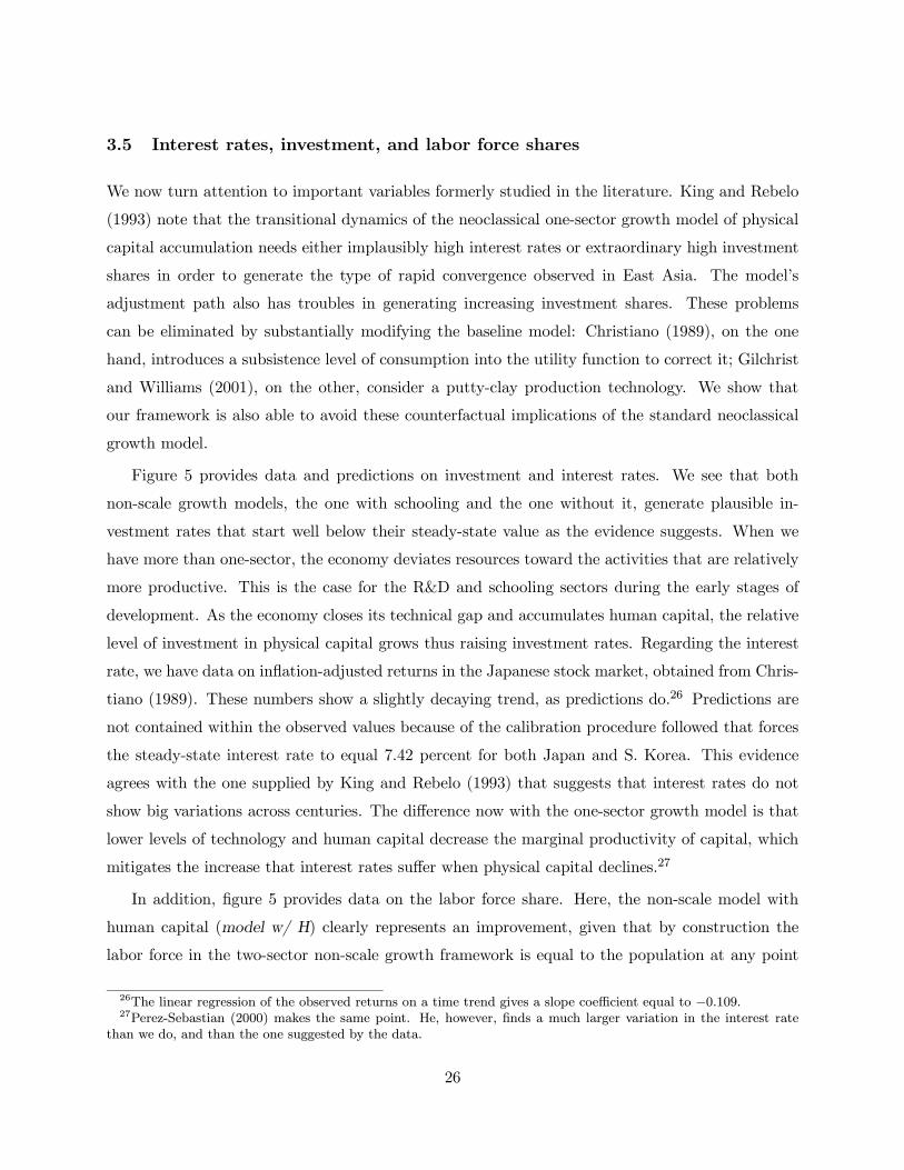
3.5 Interest rates, investment, and labor force shares

We now turn attention to important variables formerly studied in the literature. King and Rebelo

(1993) note that the transitional dynamics of the neoclassical one-sector growth model of physical

capital accumulation needs either implausibly high interest rates or extraordinary high investment

shares in order to generate the type of rapid convergence observed in East Asia. The model’s

adjustment path also has troubles in generating increasing investment shares. These problems

can be eliminated by substantially modifying the baseline model: Christiano (1989), on the one

hand, introduces a subsistence level of consumption into the utility function to correct it; Gilchrist

and Williams (2001), on the other, consider a putty-clay production technology. We show that

our framework is also able to avoid these counterfactual implications of the standard neoclassical

growth model.

Figure 5 provides data and predictions on investment and interest rates. We see that both

non-scale growth models, the one with schooling and the one without it, generate plausible in-

vestment rates that start well below their steady-state value as the evidence suggests. When we

have more than one-sector, the economy deviates resources toward the activities that are relatively

more productive. This is the case for the R&D and schooling sectors during the early stages of

development. As the economy closes its technical gap and accumulates human capital, the relative

level of investment in physical capital grows thus raising investment rates. Regarding the interest

rate, we have data on inflation-adjusted returns in the Japanese stock market, obtained from Chris-

tiano (1989). These numbers show a slightly decaying trend, as predictions do.26 Predictions are

not contained within the observed values because of the calibration procedure followed that forces

the steady-state interest rate to equal 7.42 percent for both Japan and S. Korea. This evidence

agrees with the one supplied by King and Rebelo (1993) that suggests that interest rates do not

show big variations across centuries. The difference now with the one-sector growth model is that

lower levels of technology and human capital decrease the marginal productivity of capital, which

mitigates the increase that interest rates suffer when physical capital declines.27

In addition, figure 5 provides data on the labor force share. Here, the non-scale model with

human capital (model w/ H) clearly represents an improvement, given that by construction the

labor force in the two-sector non-scale growth framework is equal to the population at any point

26The linear regression of the observed returns on a time trend gives a slope coefficient equal to −0.109.27Perez-Sebastian (2000) makes the same point. He, however, finds a much larger variation in the interest rate

than we do, and than the one suggested by the data.

26

in time.28 We see that predictions replicate fairly well the main patterns. In S. Korea the labor

force share starts far below its steady state value and grows monotonically, reflecting the return

of student to the labor force. In Japan the labor force share at impact is below the balanced

growth path and then overshoots. The overshooting is the result of the relatively high Japanese

average educational attainment in 1960 which after a few periods leads the economy to borrow

labor from the schooling sector and invest heavily on the final output and R&D activities in order

to accumulate capital and close the big technical gap at a faster rate.

Finally, we can appreciate in all figures that the main differences between the models occur far

from the steady state. This is why in the Japanese case both models offer more similar predictions

along the adjustment path — Japan in 1960 was much closer to the steady state than S. Korea

in 1963. This finding suggests that focusing on the asymptotic speed of convergence implied by

different models may not be very informative about its overall performance to explain convergence

episodes. We have shown that even though all of the models considered deliver similar asymptotic

speeds of convergence that are consistent with empirical estimates, only the non-scale growth model

with schooling successfully replicates important patterns of the Japanese and S. Korean experiences.

4 Conclusion

In this paper, we have constructed a non-scale growth model of endogenous technological change,

physical capital accumulation, and human capital formation. The goal has been to study the

model’s implications once the complementarity between technology and human capital commonly

found by the empirical literature is taken into account. In order to compare the model predictions

to the data, we have introduced human capital following the Mincerian approach suggested in recent

papers. Furthermore, we have developed a law of motion for the average educational attainment

that allows for endogenous human capital formation, and preserves the non-scale nature of the

model.

We have shown that the asymptotic speed of convergence of per-worker output predicted by the

model is consistent with the evidence. Interestingly, we have found that the introduction of human

capital makes the asymptotic speed of convergence much less sensitive to external shocks such

28Observed labor participation rates depend on the interval of age during which people can legally provide laborservices. In our model, however, people can work all along their lives. The magnitudes shown by the data and by thepredictions are therefore quite different. In order to facilitate visual comparison, we measure labor shares relative totheir 1990 value. Another problem is that the actual evolution of the labor force share reflects other things than justmovements between the production and schooling sectors, such as the increasing relative participation of women, etc.Unfortunately, solving this problem is no easy task.

27

as policy actions, which is consistent with Barro and Sala-i-Martin’s (1995) result that estimated

convergence speeds do not vary much across different region groups that belong to developed

nations. But unlike the interpretation that the literature has assigned to Barro and Sala-i-Martin’s

finding, we can not conclude that policy actions have a small effect on the convergence speed,

because non-scale growth frameworks deliver speeds of convergence that can vary over time. More

importantly, we have shown that a model that delivers an asymptotic speed of convergence that

complies better with empirical estimates does not necessarily provide a better description of the

convergence process; a careful study of different adjustment paths starting far away from the

balanced growth path is required to determine if this is the case.

Regarding this last point, we have shown that unlike the standard one-sector neoclassical growth

model and the two-sector non-scale growth model, the framework presented in this paper is fairly

successful in replicating the growth experiences of Japan and S. Korea, including important changes

in the output growth-rate trend. Moreover, this is achieved by generating adjustment paths for

interest rates, investment rates, and labor force shares that are in general agreement with observa-

tion.

Finally, we have shown that the hypothesis proposed in previous literature that the enhanc-

ing effect of human capital on technology-adoption is sufficient to reproduce the growth patterns

shown by East Asian miracle countries does not necessarily hold in a more structural model. Our

results imply that taking into account labor reallocations across sectors is crucial to replicating the

Japanese and S. Korean experiences.

Our paper is not without limitations. The model predicts enrollment rates that are larger

than their empirical counterparts. This suggests that the model predictions could be improved

if the accumulation of human capital would not necessarily imply the transfer of resources from

the final-output sector. Future research could introduce leisure in the utility function, or allow

for home-production. Alternatively, we could permit human capital formation though learning-

by-doing or on-the-job training. Another extension could consist of introducing different human

capital technologies for final output and R&D labor, although further research is clearly necessary

in determining the appropriate weights to be assigned to the effectiveness of human capital in

different sectors.

In a general sense, we interpret our results as suggesting that a successful model of economic

growth and development should include both technological progress and human capital accumulation

as necessary engines, and the endogenous outcome of the economic system. It is shown that the

28

value added from pursuing such model greatly exceeds the added complexity. In a more specific

sense, our results suggest that the technology-human capital complementarity and the subsequent

labor reallocation are crucial components in the making of miracles.

29

A Data Appendix

The data and programs used in this paper are available by the authors upon request.

• Income (GDP), and investment rates [Source: PWT 5.6]

Cross-country real GDP per worker (chain index), real GDP per capita (chain index), and real

investment shares are taken from the Penn World Tables, Version 5.6 (PWT 5.6) as described in

Summer and Heston (1991). All of the series are expressed in 1985 international prices. This data

set is available on-line at: http://datacentre.chass.utoronto.ca/pwt/index.html.

• Labor force [Source: PWT 5.6]

The cross-country data set on the labor force is calculated from the GDP per capita and GDP per

worker series. Worker for this variable is usually a census definition based on economically active

population.

• Physical capital stocks [Source: STARS (World Bank), and PWT 5.6]

Physical capital comes from PWT 5.6. However, this data set reports physical capital starting in

1965. To obtain stocks from 1963 for S. Korea, and from 1960 for Japan, we used the growth rates

implied by the STARS physical capital data to deflate the 1965 PWT 5.6 numbers.

• Education [Source: STARS (World Bank)]

Annual data on educational attainment are the sum of the average number of years of primary,

secondary and tertiary education in labor force. These series were constructed from enrollment

data using the perpetual inventory method, and they were adjusted for mortality, drop-out rates

and grade repetition. For a detailed discussion on the sources and methodology used to build this

data set see Nehru, Swanson, and Dubey (1995).

• Interest rates [Source: Christiano (1989)]

Real rates of return on physical capital for Japan are approximated using inflation-adjusted returns

in the Japanese stock market. More specifically, Christiano (1989) adjusts nominal returns using

the price deflator for personal consumption expenditure from the last quarter of the previous year

to the last quarter of the current year, from data contained in Annual Report on National Accounts,

and Report on National Accounts from 1955 to 1969. Both data sets were published in 1989 by

the Economic Planning Agency in Japan.

30

References

Amsden A., “Diffusion and Development: The Late—Industrializing Model and Greater East Asia,”AEA Papers and Proceedings, 81:282-286, 1991.

Baark, E., “The Accumulation of Technology: Capital Goods Production in Developing CountriesRevisited,”World Development, 19:903-914, 1991.

Barro, R.J. and Lee, J., “International Data on Educational Attainment: Updates and Implica-tions,” working paper no. 42, Center for International Development at Harvard University,April 2000.

Barro, R.J. and Sala-i-Martin, X., Economic Growth, Macmillan, New York, NY, 1995.

Bils, M. and Klenow, P., “Does Schooling Cause Growth?” American Economic Review, 90:1160-1183, 2000.

Caballero, R.J., and Jaffe, A.B., “How High are the Giants’ Shoulders?,” in Olivier Blanchardand Stanley Fischer,eds., NBERMacroeconomics Annual, Cambridge, MA: MIT Press, 15-74,1993.

Caselli, F., and W. J. Coleman II, “Cross-Country Technology Diffusion: The Case of Computers,”American Economic Review: Papers and Proceedings, 91:328-335, 2001.

Coe, D., and Helpman, E., “International R&D Spillovers,” European Economic Review, 39:859-887, 1995.

Coe, D., Helpman, E. and Hoffmaister, A., “North-South R&D Spillovers,” Economic Journal,107:134-149, 1997.

Christiano, L., “Understanding Japan’s Saving Rate: The Reconstruction Hypothesis,” FederalReserve of Minneapolis Quarterly Review, 2:10-29, 1989.

Dinopoulos, E. and Thompson P., “Schumpeterian Growth Without Scale Effects,” Journal ofEconomic Growth, 3:313-337, 1998.

Easterly, W., and R. Levine, “Africa’s Growth Tragedy: Policies and Ethnic Divisions,” QuarterlyJournal of Economics, 112:1202-1250, 1997.

Eicher, T., “Interaction Between Endogenous Human Capital and Technological Change,” Reviewof Economic Studies, 63:127-144, 1996.

Eicher, T., and Turnovsky, S., “A Generalized Model of Economic Growth,” Economic Journal,109:394-415, 1999a.

Eicher, T., and Turnovsky, S., “Convergence in a Two-Sector Non-Scale Growth Model,” Journalof Economic Growth, 4:413-429, 1999b.

Eicher, T., and Turnovsky, S., “Transition Dynamics in Non-Scale Models,” Journal of EconomicDynamics and Control, 25:85-113, 2001.

Funke, M. and Strulik, H., “On Endogenous Growth with Physical Capital, Human Capital andProduct Variety,” European Economic Review, 44:491-515, 2000.

Gilchrist, S., and J.C. Williams, “Transitional Dynamics in Vintage Capital Models: Explainingthe Postwar Catch-Up of Germany and Japan,” mimeo, Boston University, 2001.

Griliches, Z., “Productivity Puzzles and R&D: Another Nonexplanation,” Journal of EconomicPerspectives, 2:9-21, 1988.

31

Hall, R. and Jones, C., “Why Do Some Countries Produce So Much More Output Per WorkerThan Others?,” Quarterly Journal of Economics, 114:83-116, 1999.

Howitt, P., “Steady-State Output Growth with Population and R&D Inputs Growing,” Journalof Political Economy, 107:715-730, 1999.

Jones, C.I., “R&D-Based Models of Economic Growth,” Journal of Political Economy, 103:759-784, 1995.

Jones, C.I., “Convergence Revisited,” Journal of Economic Growth, 2:131-153, 1997.

Jones, C.I., “Sources of U.S. Economic Growth in a World of Ideas,” American Economic Review,forthcoming.

Jones, C.I, and J. Williams, “Too Much of a Good Thing: The Economics of Investment in R&D,”Journal of Economic Growth, 65-85, 2000.

Jovanovic, J. and Rob, R., “Solow vs. Solow,” working paper, NYU, 1999.

Judd, K, “Projections Methods for Solving Aggregate Growth Models,” Journal of EconomicTheory, 58:410-452, 1992.

Keller, Wolfgang, “Absorptive capacity: On the creation and acquisition of technology in devel-opment,” Journal of Development Economics, 49:199-227, 1996.

King, R. and Rebelo, S., “Transitional Dynamics and Economic Growth in the NeoclassicalModel,” American Economic Review, 83:908-931, 1993.

Klenow, P. and Rodriguez-Clare, A., “Economic Growth: A Review Essay,” Journal of MonetaryEconomics, 40:597-617, 1997.

Kortum, S., “Equilibrium R&D and the Decline in the Patent-R&D Ratio; U.S. Evidence,” Amer-ican Economic Review: Papers and Proceedings 83, 450-457, 1993.

Krueger, A. and Lindahl, M., “Education for Growth: Why and for Whom?,” Journal of EconomicLiterature, 39:1101-1136, 2001.

Lau, M-L, and Wan, H., “On the Mechanism of Catching Up,” European Economic Review38:952-963, 1994.

Lloyd-Ellis, H., and Roberts, J., “Twin Engines of Growth,” mimeo, University of Toronto, 2000.

Lucas, R., “Making a Miracle,” Econometrica, 61:251-272, 1993.

Minami, R., The Economic Development of Japan, St. Martin’s Press, New York, 1994.

Mincer, J., Schooling, Experience and Earnings, Columbia University Press, 1974.

Mulligan C.B., and Sala-i-Martin, X., “Measuring Aggregate Human Capital,” Journal of Eco-nomic Growth, 5:215-252, 2000.

Nelson, R. and Pack, H., “The Asian Miracle and Modern Growth Theory,” Economic Journal,109:416-436, 1999.

Nelson, R. and Phelps, E., “Investment in Humans, Technological Diffusion, and EconomicGrowth,” American Economic Review, 56:69-83, 1966.

Nehru, V., Swanson, E. and Dubey, A., “A new database on human capital stocks in develop-ing and industrial countries: sources, methodology and results,” Journal of DevelopmentEconomics, 46:379-401, 1995.

32

Ortigueira, S., and M. S. Santos, “On the Speed of Convergence in Endogenous Growth Models,”American Economic Review, 87:383-399, 1997.

Ozawa, “Macroeconomic Factors Affecting Japan’s Technology Inflows and Outflows: The PostwarExperience,” in International Technology Transfer: Concepts, Measures, and Comparisons,edited by N. Rosenberg and C. Frischtak, Praeger Publishers, 1985.

Parente, S.L. and Prescott, E.C., “Barriers to Technology Adoption and Development.” Journalof Political Economy, 102:298-321, 1994.

Perez-Sebastian, F., “Transitional Dynamics in an R&D-Based Growth Model with Imitation:Comparing its Predictions to the Data,” Journal of Monetary Economics, 42:437-461, 2000.

Psacharopoulos, G., “Returns to Investment in Education: A Global Update,” World Develop-ment, 22:1325-1343, 1994.

Restuccia, D., “Barriers to Capital Accumulation in a Model of Technology Adoption and School-ing,” working paper, University of Toronto, 2001.

Romer, P., “Endogenous Technological Change,” Journal of Political Economy, 98:S71-103, 1990.

Santos, M., “Accuracy of Numerical Solutions Using the Euler Equation Residuals,” Econometrica,forthcoming.

Segerstrom, P. S., “Endogenous Growth Without Scale Effects,” American Economic Review,88:1290-1310, 1998.

Stokey, N., “Learning by Doing and the Introduction of New Goods,” Journal of Political Economy,99:145-176, 1988.

Summer, R. and Heston, A., “The Penn World Table (Mark 5): An Expanded Set of InternationalComparisons: 1950-1988,” Quarterly Journal of Economics, 106:327-368, 1991.

Temple, J.R.W., “Robustness Test of the Augmented Solow Model,” Journal of Applied Econo-metrics, 13:361-375, 1998.

Young, A. “Growth without Scale Effects,” Journal of Political Economy, 106:41-63, 1998.

33