Embed Size (px)
Citation preview
HSCTM-2D, A FINITE ELEMENT MODEL FOR DEPTH-AVERAGED HYDRODYNAMICS, SEDIMENT AND
CONTAMINANT TRANSPORT
By
Earl J. Hayter1,4, Mary A. Bergs2, Ruochuan Gu3,Steve C. McCutcheon4, S. Jarrell Smith1,5, and Holly J. Whiteley1
1Department of Civil EngineeringClemson University
Clemson, South Carolina 29634-0911
2Department of Civil EngineeringUniversity of ToledoToledo, Ohio 43606
3Department of Civil EngineeringIowa State University
Ames, Iowa 50010
4National Exposure Research LaboratoryEcosystems Research Division
U. S. Environmental Protection AgencyAthens, Georgia 30605
5U.S. Army Engineer Waterways Experiment StationCoastal Engineering Research Center
P.O. Box 631Vicksburg, Mississippi 39180
NATIONAL EXPOSURE RESEARCH LABORATORYOFFICE OF RESEARCH AND DEVELOPMENT
U. S. ENVIRONMENTAL PROTECTION AGENCYATHENS, GEORGIA 30605

DISCLAIMER
The information in this document has been funded wholly or in part by the United States Environmental Protection Agency under Cooperative Agreement CR819025-02-1 to Clemson University. It has been subjected to the Agency's peer and administrative review, and it has been approved for publication as an EPA document. Mention of trade names or commercial products does not constitute endorsement or recommendation for use.
ii
FOREWORD
As environmental controls become more costly to implement and the penalties of judgement errors become more severe, environmental quality management requires more efficient analytical tools based on greater knowledge of the environmental phenomena to be managed. As part of this Laboratory's research on the occurrence, movement, transformation, impact, and control of environmental contaminants, the Assessment Branch develops management or engineering tools to help pollution control officials achieve water quality goals in impoundments, streams, and estuaries.
Clays and other cohesive sediments may influence water quality in estuaries by affecting aquatic life, by providing a large assimilative capacity, and by acting as a transporting mechanism for dissolved and particulate pollutants. In fact, the bulk of the pollution load in an estuary is quite often adsorbed to cohesive sediments rather than being dissolved in the water column. The assimilation and storage of contaminants in bottom sediments, then, is an important component of any water quality evaluation. The HSCTM-2D model addresses the movement (or non-movement) of bottom sediments and thereby assists in predicting the fate of pesticides and other organic chemicals, heavy metals, and other adsorbed contaminants.
Rosemarie C. Russo, Ph.D. Director National Exposure Research Laboratory Ecosystems Research Division Athens, Georgia
iii
ABSTRACT
HSCTM-2D (Hydrodynamic, Sediment and Contaminant Transport Model) is a finite element modeling system for simulating two-dimensional, vertically-integrated, surface water flow (typically riverine or estuarine hydrodynamics), sediment transport, and contaminant transport. The modeling system consists of two modules, one for hydrodynamic modeling (HYDRO2D) and the other for sediment and contaminant transport modeling (CS2D). One example problem is included. The HSCTM-2D modeling system may be used to simulate both short term (less than 1 year) and long term scour and/or sedimentation rates and contaminant transport and fate in vertically well mixed bodies of water.
HYDRO2D solves the equations of motion and continuity for nodal depth-averaged horizontal velocity components and flow depths. The effects of bottom, internal and surface shear stresses, horizontal salinity gradients, and the Coriolis force are represented in the equations of motion.
CS2D solves the advection-dispersion equation for nodal vertically-integrated concentrations of suspended sediment, dissolved and sorbed contaminants, and bed surface elevations. The processes of dispersion, aggregation, erosion, deposition, adsorption and desorption are simulated. A layered bed model is used in simulating bed formation and subsequent erosion. Sediment bed structure (density and shear strength profiles, thickness and elevation), net change in bed elevation and net vertical mass flux of sediment over an interval of time (e.g., over a certain number of tidal cycles), average amount of time sediment particles are in suspension, and the downward flux of sediment onto the bed are calculated for each element.
HSCTM-2D can be run in an uncoupled or semi-coupled mode. In the uncoupled mode, HYDRO2D is run separately from CS2D. In the semi-coupled mode, HYDRO2D and CS2D are run in the following fashion. First, HYDRO2D calculates the flow field for the current time step. Second, the predicted flow field is used in CS2D to calculate the transport of sediments and contaminants during the same time step. HYDRO2D is run at every time step to update the flow field to account for predicted changes in nodal flow depths due to erosion and deposition. In addition, HSCTM-2D has a default option that will allow the user to make relative comparisons between sites or designs with limited data. To obtain a quantitative analysis, the user must run the non-default option with a complete set of data.
This report was written cooperatively in partial fulfillment of cooperative agreement with Clemson University under the sponsorship of the U.S. Environmental Protection Agency. This report covers a period from October 1991 to September 1994, and work was completed as of May 1995.
iv
TABLE OF CONTENTS
Page
DISCLAIMER . . . . . . . . . . . . . . . . . . . . . . . . . . . . . . . . . . . . . . . . . . . . . . . . . . . . . . . . . . . . . . . ii FOREWORD . . . . . . . . . . . . . . . . . . . . . . . . . . . . . . . . . . . . . . . . . . . . . . . . . . . . . . . . . . . . . . . . iii ABSTRACT . . . . . . . . . . . . . . . . . . . . . . . . . . . . . . . . . . . . . . . . . . . . . . . . . . . . . . . . . . . . . . . . iv FIGURES . . . . . . . . . . . . . . . . . . . . . . . . . . . . . . . . . . . . . . . . . . . . . . . . . . . . . . . . . . . . . . . . . . ix TABLES . . . . . . . . . . . . . . . . . . . . . . . . . . . . . . . . . . . . . . . . . . . . . . . . . . . . . . . . . . . . . . . . . . . xii ABBREVIATIONS AND SYMBOLS . . . . . . . . . . . . . . . . . . . . . . . . . . . . . . . . . . . . . . . . . . . xiii ACKNOWLEDGMENTS . . . . . . . . . . . . . . . . . . . . . . . . . . . . . . . . . . . . . . . . . . . . . . . . . . . . . xix
1 INTRODUCTION . . . . . . . . . . . . . . . . . . . . . . . . . . . . . . . . . . . . . . . . . . . . . . . . . . . . . . . 1 1.1 EXPERIENCE REQUIRED TO USE HSCTM-2D . . . . . . . . . . . . . . . . . . . . . . . 1 1.2 SEDIMENTATION-RELATED PROBLEMS IN SURFACE WATERS . . . . . 2 1.3 CONTAMINATION PROBLEMS IN SURFACE WATERS . . . . . . . . . . . . . . 2 1.4 MODEL DESCRIPTION . . . . . . . . . . . . . . . . . . . . . . . . . . . . . . . . . . . . . . . . . . . 4
1.4.1 Approach to the Problems . . . . . . . . . . . . . . . . . . . . . . . . . . . . . . . . . . . . . 4 1.4.2 Overview of the Modeling System . . . . . . . . . . . . . . . . . . . . . . . . . . . . . . 5
1.5 ORGANIZATION OF THE DOCUMENT . . . . . . . . . . . . . . . . . . . . . . . . . . . . . 8
2 MODEL DEVELOPMENT, DISTRIBUTION AND SUPPORT . . . . . . . . . . . . . . . . . . 9
3 THEORY . . . . . . . . . . . . . . . . . . . . . . . . . . . . . . . . . . . . . . . . . . . . . . . . . . . . . . . . . . . . 10 3.1 ESTUARIAL DYNAMICS . . . . . . . . . . . . . . . . . . . . . . . . . . . . . . . . . . . . . . . . 10
3.1.1 General Description . . . . . . . . . . . . . . . . . . . . . . . . . . . . . . . . . . . . . . . . . 10 3.1.2 Governing Equations . . . . . . . . . . . . . . . . . . . . . . . . . . . . . . . . . . . . . . . . 11
3.1.2.1 Coordinate System . . . . . . . . . . . . . . . . . . . . . . . . . . . . . . . . . . . 11 3.1.2.2 Equations of Motion . . . . . . . . . . . . . . . . . . . . . . . . . . . . . . . . . . 11
3.2 COHESIVE SEDIMENT TRANSPORT . . . . . . . . . . . . . . . . . . . . . . . . . . . . . . 14 3.2.1 Description and Properties of Cohesive Sediments . . . . . . . . . . . . . . . . 14
3.2.1.1 Composition . . . . . . . . . . . . . . . . . . . . . . . . . . . . . . . . . . . . . . . . 14 3.2.1.2 Structure . . . . . . . . . . . . . . . . . . . . . . . . . . . . . . . . . . . . . . . . . . . 15 3.2.1.3 Interparticle Forces . . . . . . . . . . . . . . . . . . . . . . . . . . . . . . . . . . . 15 3.2.1.4 Cation Exchange Capacity . . . . . . . . . . . . . . . . . . . . . . . . . . . . . 16
3.2.2 Estuarial Cohesive Sediment Transport . . . . . . . . . . . . . . . . . . . . . . . . . . 17 3.2.2.1 Overview . . . . . . . . . . . . . . . . . . . . . . . . . . . . . . . . . . . . . . . . . . 17 3.2.2.2 Sediment Bed . . . . . . . . . . . . . . . . . . . . . . . . . . . . . . . . . . . . . . . 19 3.2.2.3 Erosion . . . . . . . . . . . . . . . . . . . . . . . . . . . . . . . . . . . . . . . . . . . . 23 3.2.2.4 Advection and Dispersion . . . . . . . . . . . . . . . . . . . . . . . . . . . . . 30 3.2.2.5 Dispersive Transport . . . . . . . . . . . . . . . . . . . . . . . . . . . . . . . . . . 31 3.2.2.6 Coagulation . . . . . . . . . . . . . . . . . . . . . . . . . . . . . . . . . . . . . . . . . 34 3.2.2.7 Aggregation . . . . . . . . . . . . . . . . . . . . . . . . . . . . . . . . . . . . . . . . 38 3.2.2.8 Settling . . . . . . . . . . . . . . . . . . . . . . . . . . . . . . . . . . . . . . . . . . . . 39
v
3.2.2.9 Deposition . . . . . . . . . . . . . . . . . . . . . . . . . . . . . . . . . . . . . . . . . . 39 3.2.2.10 Consolidation . . . . . . . . . . . . . . . . . . . . . . . . . . . . . . . . . 55
3.3 COHESIONLESS SEDIMENT TRANSPORT . . . . . . . . . . . . . . . . . . . . . . . . . 59 3.4 CONTAMINANT TRANSPORT . . . . . . . . . . . . . . . . . . . . . . . . . . . . . . . . . . . . 63
4 FINITE ELEMENT METHOD . . . . . . . . . . . . . . . . . . . . . . . . . . . . . . . . . . . . . . . . . . . . 70 4.1 INTRODUCTORY NOTE . . . . . . . . . . . . . . . . . . . . . . . . . . . . . . . . . . . . . . . . . 70 4.2 DESCRIPTION . . . . . . . . . . . . . . . . . . . . . . . . . . . . . . . . . . . . . . . . . . . . . . . . . 71
4.2.1 Interpolation Functions . . . . . . . . . . . . . . . . . . . . . . . . . . . . . . . . . . . . . . 71 4.2.2 Method of Weighted Residuals . . . . . . . . . . . . . . . . . . . . . . . . . . . . . . . . 75 4.2.3 Discretization of Physical System . . . . . . . . . . . . . . . . . . . . . . . . . . . . . . 75
4.3 FINITE ELEMENT FORMULATION . . . . . . . . . . . . . . . . . . . . . . . . . . . . . . . 76 4.3.1 Hydrodynamic Equations . . . . . . . . . . . . . . . . . . . . . . . . . . . . . . . . . . . . 76 4.3.2 Sediment and Contaminant Transport Equations . . . . . . . . . . . . . . . . . . 78 4.3.3 Boundary Conditions . . . . . . . . . . . . . . . . . . . . . . . . . . . . . . . . . . . . . . . . 79 4.3.4 Equations Solver . . . . . . . . . . . . . . . . . . . . . . . . . . . . . . . . . . . . . . . . . . . 80
5 DESCRIPTION OF THE MODELING SYSTEM . . . . . . . . . . . . . . . . . . . . . . . . . . . . . 81 5.1 SYSTEM COMPONENTS . . . . . . . . . . . . . . . . . . . . . . . . . . . . . . . . . . . . . . . . 81 5.2 HYDRODYNAMIC MODULE . . . . . . . . . . . . . . . . . . . . . . . . . . . . . . . . . . . . . 82 5.3 COHESIVE SEDIMENT TRANSPORT MODULE . . . . . . . . . . . . . . . . . . . . . 82
5.3.1 Bed Schematization . . . . . . . . . . . . . . . . . . . . . . . . . . . . . . . . . . . . . . . . . 83 5.3.2 Erosion Algorithm . . . . . . . . . . . . . . . . . . . . . . . . . . . . . . . . . . . . . . . . . . 87 5.3.3 Dispersion Algorithm . . . . . . . . . . . . . . . . . . . . . . . . . . . . . . . . . . . . . . . 90 5.3.4 Deposition Algorithm . . . . . . . . . . . . . . . . . . . . . . . . . . . . . . . . . . . . . . . 94
6 DATA COLLECTION AND MODEL CALIBRATION . . . . . . . . . . . . . . . . . . . . . . . . 99 6.1 DATA COLLECTION AND ANALYSIS . . . . . . . . . . . . . . . . . . . . . . . . . . . . . 99
6.1.1 Field Data Collection Program . . . . . . . . . . . . . . . . . . . . . . . . . . . . . . . . 99 Hydrographic Survey . . . . . . . . . . . . . . . . . . . . . . . . . . . . . . . . . 99 Sediment Sampling Using Corers . . . . . . . . . . . . . . . . . . . . . . . . 101 Measurement of Suspended Concentration, Salinity and Temperature . . . . . . . . . . . . . . . . . . . . . . . . . . . . . . . . . . . . . . . . 101 Determination of Sediment Settling Velocity . . . . . . . . . . . . . . . 103
6.1.2 Laboratory Testing Program . . . . . . . . . . . . . . . . . . . . . . . . . . . . . . . . . . 103 Properties of Undisturbed Sediment Cores . . . . . . . . . . . . . . . . 103 Properties of Original Settled Bed . . . . . . . . . . . . . . . . . . . . . . . 103 Properties of New Deposits . . . . . . . . . . . . . . . . . . . . . . . . . . . . 104 Aggregate Shear Strength and Density . . . . . . . . . . . . . . . . . . . . 104 Fluid Composition . . . . . . . . . . . . . . . . . . . . . . . . . . . . . . . . . . . 105 Composition and Cation Exchange Capacity of the Sediment . . 105
6.2 MODEL CALIBRATION . . . . . . . . . . . . . . . . . . . . . . . . . . . . . . . . . . . . . . . . . 106 6.2.1 Hydrodynamic Module . . . . . . . . . . . . . . . . . . . . . . . . . . . . . . . . . . . . . . 106 6.2.2 Sediment Transport Module . . . . . . . . . . . . . . . . . . . . . . . . . . . . . . . . . . 107
vi
7 HSCTM-2D USER INSTRUCTIONS . . . . . . . . . . . . . . . . . . . . . . . . . . . . . . . . . . . . . . 108 7.1 MODELING SYSTEM LIMITATIONS . . . . . . . . . . . . . . . . . . . . . . . . . . . . . . 108
7.1.1 Limitations of the Hydrodynamic Module . . . . . . . . . . . . . . . . . . . . . . . 109 7.2 USER INSTRUCTIONS . . . . . . . . . . . . . . . . . . . . . . . . . . . . . . . . . . . . . . . . . . 110 7.3 DATA INPUT FOR MAIN PROGRAM OF HSCTM-2D . . . . . . . . . . . . . . . . 111 7.4 SYSTEM DATA OUTPUT . . . . . . . . . . . . . . . . . . . . . . . . . . . . . . . . . . . . . . . . 111
7.4.1 Hydrodynamic Module . . . . . . . . . . . . . . . . . . . . . . . . . . . . . . . . . . . . . . 111 7.4.2 Sediment Transport Module . . . . . . . . . . . . . . . . . . . . . . . . . . . . . . . . . . 111 7.4.3 Contaminant Transport Module . . . . . . . . . . . . . . . . . . . . . . . . . . . . . . . 112
8 DATA INPUT REQUIREMENTS . . . . . . . . . . . . . . . . . . . . . . . . . . . . . . . . . . . . . . . . . 114 8.1 GRID GENERATION . . . . . . . . . . . . . . . . . . . . . . . . . . . . . . . . . . . . . . . . . . . . 114 8.2 DATA INPUT FOR MAIN PROGRAM OF HSCTM-2D . . . . . . . . . . . . . . . . 115
8.2.1 Input/Output Filenames . . . . . . . . . . . . . . . . . . . . . . . . . . . . . . . . . . . . . . 115 8.3 HYDRODYNAMIC MODULE - DATA INPUT . . . . . . . . . . . . . . . . . . . . . . . 117 8.4 SEDIMENT/CONTAMINANT TRANSPORT MODULE - DATA INPUT . . 117
8.4.1 Data Set A: Job Control Cards . . . . . . . . . . . . . . . . . . . . . . . . . 117 8.4.2 Data Set B: Job Control Parameters . . . . . . . . . . . . . . . . . . . . . 119 8.4.3 Data Set C: Transient Problem Input . . . . . . . . . . . . . . . . . . . . . 121 8.4.4 Data Set D: Water and Sediment Properties . . . . . . . . . . . . . . . 122 8.4.5 Data Set E: Initial Concentration Field . . . . . . . . . . . . . . . . . . . 126 8.4.6 Data Set F: Original Settled Bed Profile . . . . . . . . . . . . . . . . . . 127 8.4.7 Data Set G: Initial Velocity Field . . . . . . . . . . . . . . . . . . . . . . . 128 8.4.8 Data Set H: Initial Dispersion Coefficients . . . . . . . . . . . . . . . . 129 8.4.9 Data Set I: Initial Settling Velocities . . . . . . . . . . . . . . . . . . . . . 130 8.4.10 Data Set J: Boundary Conditions . . . . . . . . . . . . . . . . . . . . . . . . 130 8.4.11 Data Set K: New Salinities . . . . . . . . . . . . . . . . . . . . . . . . . . . . 131 8.4.12 Data Set L: Dynamic Input . . . . . . . . . . . . . . . . . . . . . . . . . . . . 131
8.5 DATA MANAGEMENT . . . . . . . . . . . . . . . . . . . . . . . . . . . . . . . . . . . . . . . . . . 132 8.6 DEFAULT OPTION . . . . . . . . . . . . . . . . . . . . . . . . . . . . . . . . . . . . . . . . . . . . . 132
9 EXAMPLE PROBLEM . . . . . . . . . . . . . . . . . . . . . . . . . . . . . . . . . . . . . . . . . . . . . . . . . 135
REFERENCES . . . . . . . . . . . . . . . . . . . . . . . . . . . . . . . . . . . . . . . . . . . . . . . . . . . . . . . . . . . . . 143
APPENDICES
A HSCTM-2D STRUCTURE . . . . . . . . . . . . . . . . . . . . . . . . . . . . . . . . . . . . . . . . . . . . . . 152 A.1 Subroutines in HYDRO2D . . . . . . . . . . . . . . . . . . . . . . . . . . . . . . . . . . . . . . . . . 152 A.2 Subroutines in CS2D . . . . . . . . . . . . . . . . . . . . . . . . . . . . . . . . . . . . . . . . . . . . . 153
B LABORATORY SEDIMENT TESTING PROGRAM . . . . . . . . . . . . . . . . . . . . . . . . . 156 B.1 Properties of Undisturbed Sediment Cores . . . . . . . . . . . . . . . . . . . . . . . . . . . . 156 B.2 Properties of Original Settled Bed . . . . . . . . . . . . . . . . . . . . . . . . . . . . . . . . . . . 156 B.3 Properties of New Deposits . . . . . . . . . . . . . . . . . . . . . . . . . . . . . . . . . . . . . . . . 157
vii

C
B.4 Fluid Composition . . . . . . . . . . . . . . . . . . . . . . . . . . . . . . . . . . . . . . . . . . . . . . . 158 B.5 Composition and Cation Exchange Capacity of the Sediment . . . . . . . . . . . . . . 158
DATA OUTPUT FOR HSCTM-2D AND DATA INPUT FOR HYDRO2D . . . . . . . . 160 C.1 HSCTM-2D Binary Output File Format . . . . . . . . . . . . . . . . . . . . . . . . . . . . . . 161 C.2 Card Image Input Data Coding Instructions for HYDRO2D . . . . . . . . . . . . . . . 162 C.3 Input Data Cards Description . . . . . . . . . . . . . . . . . . . . . . . . . . . . . . . . . . . . . . . 173
viii
FIGURES
Fig. No. Page
1.1 Flowchart of HSCTM-2D Modeling System . . . . . . . . . . . . . . . . . . . . . . . . . . . . . . . . . . 7
3.1 Coordinate System . . . . . . . . . . . . . . . . . . . . . . . . . . . . . . . . . . . . . . . . . . . . . . . . . . . . . 11
3.2 Schematic Representation of Transport and Shoaling Processes in the Mixing Zone of a Stratified Estuary (after Mehta and Hayter 1981). . 18
3.3 Time and Depth Variation of Suspended Sediment Concentration in the Savannah River Estuary (after Krone 1972). . . . . . . . . . . . . . . . . . . . . . . . . . . . . . . . . . . . . . . . . . . 20
3.4 Schematic Representation of the Physical States of Cohesive Sediments in Estuarial Mixing Zone (after Mehta et al. 1982a). . . . . . . . . . . . . . . . . . . . . . . . . . . . . . . . . . . . . . 21
3.5 Bed Shear Strength Profiles as Functions of Salinity. . . . . . . . . . . . . . . . . . . . . . . . . . . 24
3.6 Relative Suspended Sediment Concentration versus Time for a Stratified Bed (after Mehta and Partheniades 1979). . . . . . . . . . . . . . . . . . . . . . . . . . . . . . . . . . . . . . . . . . . . . 27
3.7 Normalized Rate of Erosion versus Normalized Excess Shear Stress Using Kaolinite in Tap Water (after Mehta et al. 1982a). . . . . . . . . . . . . . . . . . . . . . . . . . . . . . 28
3.8 Internal Circulation in a Partially Stratified Estuary. (a) A Transverse Section; (b) A Vertical Section (after Fischer et al. 1979). . . . . . . . . . . . . . . . . . . . . . . . . . . . . . . . . 36
3.9 Illustration of Wind-Induced Circulation (adapted from Fischer et al. 1979). . . . . . . . . 37
3.10 Comparison of the Collision Functions for Brownian, Shear and Differential-Sedimentation Coagulation (after Hunt 1980). . . . . . . . . . . . . . . . . . . . . . . . . . . . . . . . . 38
3.11 Ratio C/Co versus Time for Kaolinite in Distilled Water (after Mehta and Partheniades 1975). . . . . . . . . . . . . . . . . . . . . . . . . . . . . . . . . . . . . . . . . . . . . . . . . . . . . . 42
3.12 Ratio Ceq/Co versus Bed Shear Stress Jb (after Mehta and Partheniades 1975). . . . . . . . 43
C *3.13 versus Jb* - 1 (after Mehta and Partheniades 1975). . . . . . . . . . . . . . . . . . . . . . . . . 45 eq
3.14 C* in Percent versus t/t50 for Kaolinite in Distilled Water (after Mehta and Partheniades 1975). . . . . . . . . . . . . . . . . . . . . . . . . . . . . . . . . . . . . . . . . . . . . . . . . . . . . . 46
ix
3.15 Log t50 versus J*b for Kaolinite in Distilled Water (after Mehta and Partheniades
1975). . . . . . . . . . . . . . . . . . . . . . . . . . . . . . . . . . . . . . . . . . . . . . . . . . . . . . . . . . . . . . . . 48
3.16 Settling Velocity versus Concentration for San Francisco Bay Mud (after Krone1962). . . . . . . . . . . . . . . . . . . . . . . . . . . . . . . . . . . . . . . . . . . . . . . . . . . . . . . . . . . . . . . . 49
3.17 Settling Velocity versus Concentration (after Thorn 1981). . . . . . . . . . . . . . . . . . . . . . . 50
3.18 Effect of Size and Settling Velocity of Elementary Particles on the CoagulationFactor of Natural Muds (after Bellessort 1973). . . . . . . . . . . . . . . . . . . . . . . . . . . . . . . . 52
3.19 Effect of Salinity on Settling Velocity of San Francisco Bay Mud (after Krone1962). . . . . . . . . . . . . . . . . . . . . . . . . . . . . . . . . . . . . . . . . . . . . . . . . . . . . . . . . . . . . . . . 53
3.20 Effect of Salinity on Settling Velocity of Avonmouth Mud (after Owen 1970). . . . . . . 54
3.21 Variation of Mean Bed Density with Consolidation Time (after Dixit 1982). . . . . . . . . 56
3.22 Variation of the Normalized Mean Bed Density versus Consolidation Time (afterDixit 1982). . . . . . . . . . . . . . . . . . . . . . . . . . . . . . . . . . . . . . . . . . . . . . . . . . . . . . . . . . . . 56
3.23 Normalized Depth Below the Surface versus Normalized Bed Bulk Density forAvonmouth, Brisbane, Grangemouth and Belawan Muds (after Dixit 1982). . . . . . . . . 57
3.24 Normalized Depth Below the Bed Surface versus Normalized Bed Bulk Density forConsolidation Times (a) Less than 48 Hours and (b) Greater than 48 Hours (afterDixit 1982). . . . . . . . . . . . . . . . . . . . . . . . . . . . . . . . . . . . . . . . . . . . . . . . . . . . . . . . . . . . 58
3.25 Normalized Bed Density Profiles for Different Bed Thicknesses. . . . . . . . . . . . . . . . . . 60
3.26 Bed Shear Strength versus Distance Below the Initial Bed Surface for VariousConsolidation Periods (after Dixit 1982). . . . . . . . . . . . . . . . . . . . . . . . . . . . . . . . . . . . . 61
3.27 Correlation of Bed Shear Strength with Bed Density (after Owen 1970). . . . . . . . . . . . 62
4.1 Global and Local Coordinates . . . . . . . . . . . . . . . . . . . . . . . . . . . . . . . . . . . . . . . . . . . . . 72
5.1 Bed Schematization Used in Bed Formation Algorithm . . . . . . . . . . . . . . . . . . . . . . . . . 85
5.2 Hypothetical Shear Strength Profile Illustrating Determination of Bed LayerThickness. . . . . . . . . . . . . . . . . . . . . . . . . . . . . . . . . . . . . . . . . . . . . . . . . . . . . . . . . . . . . 86
5.3 Apparent Settling Velocity Description in Domains Defined by SuspendedSediment Concentration and Bed Shear Stress . . . . . . . . . . . . . . . . . . . . . . . . . . . . . . . . 95
x
6.1 A Plot of Raw Viscometer Data Obtained from the U.S. Army Corps of EngineersPhiladelphia District Sample (after Krone 1963). . . . . . . . . . . . . . . . . . . . . . . . . . . . . . . 106
9.1 Reach of Winyah Bay, South Carolina modeled. . . . . . . . . . . . . . . . . . . . . . . . . . . . . . . 138
9.2 Finite Element Grid used in the HSCTM-2D Modeling. . . . . . . . . . . . . . . . . . . . . . . . . 139
9.3 Velocity Vectors During Simulated Ebb Tide . . . . . . . . . . . . . . . . . . . . . . . . . . . . . . . . 140
9.4 Constant Length (indicate flow direction only) Velocity Vectors in the Marina During Ebb Tide . . . . . . . . . . . . . . . . . . . . . . . . . . . . . . . . . . . . . . . . . . . . . . . . . . . . . . . 141
9.5 Sedimentation Contours (mm) after 5 Day Simulation . . . . . . . . . . . . . . . . . . . . . . . . . . 142
xi
TABLES
Page
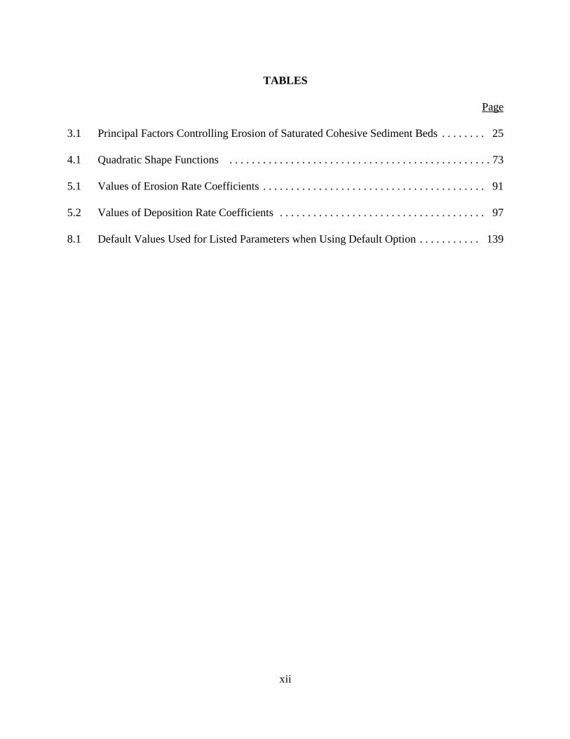
3.1 Principal Factors Controlling Erosion of Saturated Cohesive Sediment Beds . . . . . . . . 25
4.1 Quadratic Shape Functions . . . . . . . . . . . . . . . . . . . . . . . . . . . . . . . . . . . . . . . . . . . . . . . 73
5.1 Values of Erosion Rate Coefficients . . . . . . . . . . . . . . . . . . . . . . . . . . . . . . . . . . . . . . . . 91
5.2 Values of Deposition Rate Coefficients . . . . . . . . . . . . . . . . . . . . . . . . . . . . . . . . . . . . . 97
8.1 Default Values Used for Listed Parameters when Using Default Option . . . . . . . . . . . 139
xii
ABBREVIATIONS AND SYMBOLS
ABBREVIATIONS
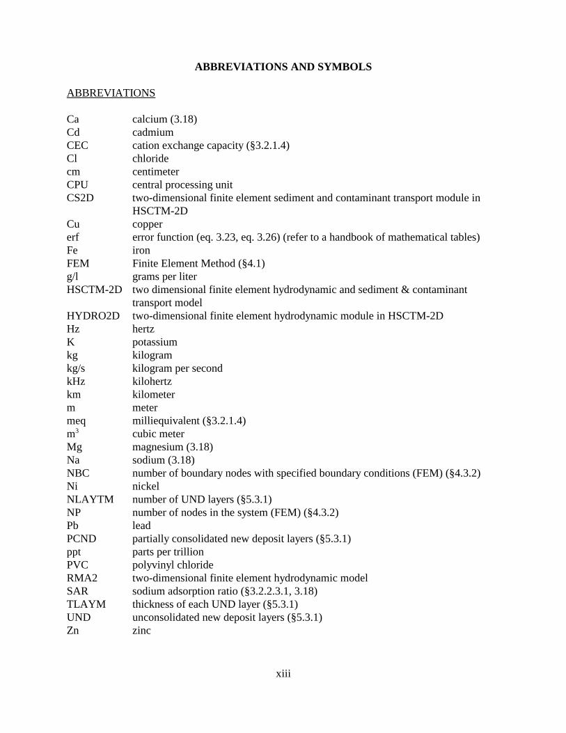
Ca calcium (3.18) Cd cadmium CEC cation exchange capacity (§3.2.1.4) Cl chloride cm centimeter CPU central processing unit CS2D two-dimensional finite element sediment and contaminant transport module in
HSCTM-2D Cu copper erf error function (eq. 3.23, eq. 3.26) (refer to a handbook of mathematical tables) Fe iron FEM Finite Element Method (§4.1) g/l grams per liter HSCTM-2D two dimensional finite element hydrodynamic and sediment & contaminant
transport model HYDRO2D two-dimensional finite element hydrodynamic module in HSCTM-2D Hz hertz K potassium kg kilogram kg/s kilogram per second kHz kilohertz km kilometer m meter meq milliequivalent (§3.2.1.4) m3 cubic meter Mg magnesium (3.18) Na sodium (3.18) NBC number of boundary nodes with specified boundary conditions (FEM) (§4.3.2) Ni nickel NLAYTM number of UND layers (§5.3.1) NP number of nodes in the system (FEM) (§4.3.2) Pb lead PCND partially consolidated new deposit layers (§5.3.1) ppt parts per trillion PVC polyvinyl chloride RMA2 two-dimensional finite element hydrodynamic model SAR sodium adsorption ratio (§3.2.2.3.1, 3.18) TLAYM thickness of each UND layer (§5.3.1) UND unconsolidated new deposit layers (§5.3.1) Zn zinc
xiii
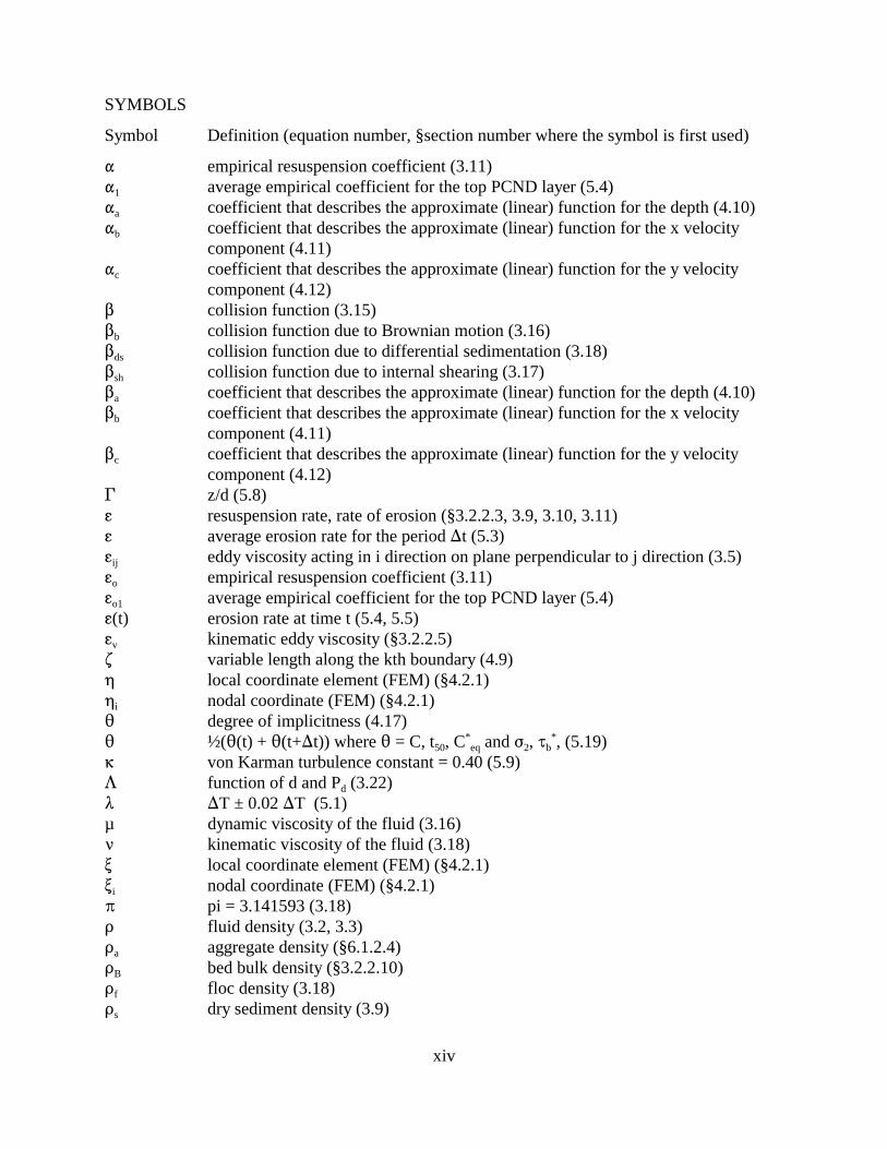
SYMBOLS
Symbol Definition (equation number, §section number where the symbol is first used)
" empirical resuspension coefficient (3.11)" average empirical coefficient for the top PCND layer (5.4)1
" coefficient that describes the approximate (linear) function for the depth (4.10) a
" coefficient that describes the approximate (linear) function for the x velocity b
component (4.11) " coefficient that describes the approximate (linear) function for the y velocity c
$$$
component (4.12)$ collision function (3.15)
b collision function due to Brownian motion (3.16)
ds collision function due to differential sedimentation (3.18)
sh collision function due to internal shearing (3.17)$ coefficient that describes the approximate (linear) function for the depth (4.10)a
$b coefficient that describes the approximate (linear) function for the x velocity component (4.11)
$ coefficient that describes the approximate (linear) function for the y velocity c
0
g
ggg
component (4.12)' z/d (5.8)g resuspension rate, rate of erosion (§3.2.2.3, 3.9, 3.10, 3.11)g average erosion rate for the period )t (5.3)
ij eddy viscosity acting in i direction on plane perpendicular to j direction (3.5)
o empirical resuspension coefficient (3.11)
o1 average empirical coefficient for the top PCND layer (5.4)g(t) erosion rate at time t (5.4, 5.5)
v kinematic eddy viscosity (§3.2.2.5). variable length along the kth boundary (4.9)0 local coordinate element (FEM) (§4.2.1)
i nodal coordinate (FEM) (§4.2.1)2 degree of implicitness (4.17)
*
>
2 ½(2(t) + 2(t+)t)) where 2 = C, t50, C*eq and F2, Jb , (5.19)
6 von Karman turbulence constant = 0.40 (5.9)7 function of d and Pd (3.22)8 )T ± 0.02 )T (5.1)µ dynamic viscosity of the fluid (3.16)< kinematic viscosity of the fluid (3.18)> local coordinate element (FEM) (§4.2.1)
i nodal coordinate (FEM) (§4.2.1)B pi = 3.141593 (3.18)D fluid density (3.2, 3.3)D aggregate density (§6.1.2.4)a
DDB bed bulk density (§3.2.2.10)
f floc density (3.18) D dry sediment density (3.9) s
xiv
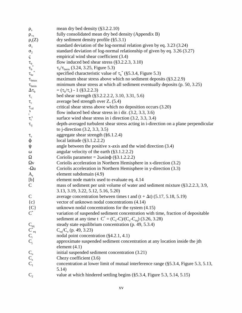
D mean dry bed density (§3.2.2.10) s
J
FF
D4s fully consolidated mean dry bed density (Appendix B)Ds(Z) dry sediment density profile (§5.3.1)
1 standard deviation of the log-normal relation given by eq. 3.23 (3.24)
2 standard deviation of log-normal relationship of given by eq. 3.26 (3.27)H empirical wind shear coefficient (3.4)
b flow induced bed shear stress (§3.2.2.3, 3.10)Jb
*
JJJ
Jb/Jbmin (3.24, 3.25, Figure 5.3)
bc* specified characteristic value of Jb
* (§5.3.4, Figure 5.3)
bmax maximum shear stress above which no sediment deposits (§3.2.2.9)
bmin minimum shear stress at which all sediment eventually deposits (p. 50, 3.25))Jb = (Jb/Jc) - 1 (§3.2.2.3)J bed shear strength (§3.2.2.2.2, 3.10, 3.31, 5.6)c
J average bed strength over Z* (5.4)c
Jcd critical shear stress above which no deposition occurs (3.20) b flow induced bed shear stress in i dir. (3.2, 3.3, 3.6)i
s
JJi surface wind shear stress in i direction (3.2, 3.3, 3.4)
ij depth-averaged turbulent shear stress acting in i-direction on a plane perpendicular to j-direction (3.2, 3.3, 3.5)
J aggregate shear strength (§6.1.2.4) s
N local latitude (§3.1.2.2.2)R angle between the positive x-axis and the wind direction (3.4)T angular velocity of the earth (§3.1.2.2.2)S Coriolis parameter = 2TsinN (§3.1.2.2.2)Sv Coriolis acceleration in Northern Hemisphere in x-direction (3.2)-Su Coriolis acceleration in Northern Hemisphere in y-direction (3.3)A element subdomain (4.9)e
[b] element node matrix used to evaluate eq. 4.14 C mass of sediment per unit volume of water and sediment mixture (§3.2.2.3, 3.9,
3.13, 3.19, 3.22, 5.12, 5.16, 5.20) C average concentration between times t and (t + )t) (5.17, 5.18, 5.19) {c} vector of unknown nodal concentrations (4.14)
C{C} unknown nodal concentrations for the system (4.15)
* variation of suspended sediment concentration with time, fraction of depositablesediment at any time t C* = (Co-C)/(Co-Ceq) (3.26, 3.28)
C steady state equilibrium concentration (p. 49, 5.3.4) eq
C* Ceq/Co (p. 49, 3.23)eq
CCi nodal point concentration (§4.2.1, 4.1)
j approximate suspended sediment concentration at any location inside the jth element (4.1)
C initial suspended sediment concentration (3.21)o
C Chezy coefficient (3.6) z
C
C1 concentration at lower limit of mutual interference range (§5.3.4, Figure 5.3, 5.13, 5.14)
2 value at which hindered settling begins (§5.3.4, Figure 5.3, 5.14, 5.15)
xv
d depth of flow (3.1)d thickness of sediment deposited per time step (§5.3.4)e
ˆ refer to equation between 5.17 and 5.18 (5.17)e
D
di, dj effective diameter of a suspended sediment particle (3.15)dNi number of particles with sizes between di and [di + )(di)] (3.15)dNj number of particles with sizes between dj and [dj + )(dj)] (3.15)D mean particle diameter in microns (§3.2.2.9)
ij (where i and j are replaced by x or y) effective sediment dispersivity tensor (3.13,5.7)
ê mean value of the scalar turbulent diffusion coefficient in the vertical direction Ez
(5.7, §5.3.3, 5.10) E´ E /ê (5.8)z
E vertical turbulent diffusion coefficient (5.9, §5.3.3, 5.10)z
f 0.845; empirical coefficient used in the consolidation algorithm to be determined by performing laboratory consolidation tests
{f} element source/sink vector (4.14)F flocculation factor (3.30, Figure 3.19){F} system source/sink array (4.15)FC collision frequency for suspended sediment particles (3.15)g constant of acceleration due to gravity (3.2, 3.3)G local shearing rate = du/dz (3.17, §3.2.2.6)H thickness of bed in Dixit experiment (Figure 3.24-Figure 3.26)H height of water in outer cylinder (Figure 6.1)H suspension depth (Figure 3.26)o
Ii counter (4.1, 7.1)
ii refer to equation 5.8 (5.7); often assumed to be a constant (§5.3.3)j counter (4.9 - 4.13, 7.1)J current time step (t = J)t) indicator (4.17)J+1 next time step (t = (J+1))t) indicator (4.17)*J* Jacobian (4.3, 4.4, 4.5)k Boltzmann constant (3.16)[k] element steady-state coefficient matrix (4.14)K inverse of the hypothetical, fully settled sediment concentration (5.15)[K] system steady-state coefficient matrix (4.15)K empirical constant (3.29, 5.14)e
L counter (4.9)m empirical power coefficient (3.29, 5.14)M erodibility constant (§3.2.2.3, Table 5.1)M(1) erodibility constant for the first layer (5.5)M´ M"Jc (2.13.10)
M{M} shape function representing flow depth (4.10)
D dry sediment mass deposited per unit bed area per element per time step (§5.3.1, 5.17)
MR sediment mass per unit bed area that is redispersed during one time stop (§5.3.2, 5.2)
xvi
x n direction cosine between the boundary normal and the x-direction (4.11, 4.12) n direction cosine between the boundary normal and the y-direction (4.11, 4.12) y
nn number of nodes forming the jth element (4.1)
N{N} shape function representing velocity (4.11)
sub shape function for node 'sub' in a given element (FEM) where sub = any subscript(§4.2.1, 4.1, 4.3, 4.4)
NE total number of elements in grid (4.9) NEC number of elements in which at least one erosion-deposition cycle occurred (7.1) NL number of element interfaces and external boundaries (4.8) NOCR number of erosion-deposition cycles that occur in the ith element over the entire
qP
simulation period (7.1)
d probability of deposition (3.19, 3.20)
i+ outward normal flux from one element (4.8) -
qqi outward normal flux from one element (4.8)
subs normal flux from source/sink on the 'sub' boundary where sub = any subscript
(4.8, 4.13) Q MC/Mt - ST = constant (4.13) r residual that results from applying the governing equations to the element
R
subdomain using the approximate value instead of the actual value (§4.2.2, 4.9)R residual that results from the use of in eq. 4.8 (4.9)
ij collision radius between di and dj size particles = di + dj (3.17)S salinity (§3.2.2.9, 5.6)S boundary of element for line integral (4.11, 4.12)e
SSL localized source/sink term for dredging and dumping (3.14)
T source/sink term (3.13, 3.14)t time (3.1)[t] temporal matrix (4.14))t time increment (4.16)()tE-D)j jth time period from occurrence of either redispersion or resuspension to
occurrence of deposition in the ith element. (7.1) t the average amount of time sediment particles are in suspension for the entire ave
tmodel simulation (7.1)
50 time at which C* = 50% (3.27) T refer to eq. 3.27 (3.26)
TT
[T] system temporal matrix (4.15))T thickness of the bed formed for each element (§5.3.1, 5.1)
dc consolidation time (§3.2.2.10)
k absolute temperature (3.16)u depth-averaged water velocity component in the x-direction (3.1)· depth-averaged velocity component in the x-direction (§5.3.3)u´ u(z) - · (5.7); velocity deviation over depth from the depth-averaged value u (5.7,
u
§5.3.3)u1 u´/u (5.8)
f shear velocity (5.9)u(z) vertical velocity profile (§5.3.3)
xvii
U root-mean-square value of u´ over the depth d (5.7); the intensity of u´ (§5.3.3) v depth-averaged velocity component in the y-direction (3.1) v depth-averaged component of the velocity in the y-direction (5.7) v´ v(z) - v (5.7); velocity deviation over depth from the depth-averaged value v
(5.7, §5.3.3) v(z) vertical velocity profile (§5.3.3) V root-mean-square value of v´ over the depth d (5.7); the intensity of v´ (§5.3.3) w integration variable (Figure 3.13, Figure 3.14) W wind speed (3.4) W reference settling velocity (5.15) r
W [median] sediment settling velocity (3.19, 3.29) s
W ´ effective settling velocity, Pd "Ws (§5.3.4, 5.12)s
y
x
W´WWWsA median settling velocity of aggregates (3.30)
sP median settling velocity of sediment particles (3.30)
s1 median sediment settling velocity in the free settling range (5.13)
s1 effective settling velocity in Range I as defined on Figure 5.3 (5.13, 5.14, 5.15)x global coordinate in a horizontal direction (§3.1.2.1)x approximation of the global coordinate x (4.2)
i global nodal point coordinate (4.2)y global coordinate in a horizontal direction (§3.1.2.1)y approximation of the global coordinate y (4.2)
i global nodal point coordinate (4.2)Y see eq. 3.24 (3.23)a
zz global coordinate in the vertical direction following the right-hand rule (§3.1.2.1)
b bed elevation (3.2, 3.3)z depth of erosion (§3.2.2.3)e
Z* the bed depth at which Jc(zb) = Jb (§5.3.2) Z depth below the initial bed surface (§3.2.2.2.2)
xviii

ACKNOWLEDGMENTS
The development of a numerical model is a time-consuming task that normally extends over a number of years. There are significant periods in the evolution of a computer code, but rarely is there a definitive end to the development. Such is the case with the HSCTM-2D code that simulates vertically-integrated hydrodynamics and the transport of both cohesionless and cohesive (silts and clays) sediment, and (at present) one inorganic contaminant.
Work on HSCTM-2D originated in 1980 with the dissertation studies of Earl Hayter in the University of Florida's Coastal & Oceanographic Engineering Department under the advisement of Professor A.J. Mehta. Mr. Hayter's research was first supported by a grant from the U.S. EPA Environmental Research Laboratory at Athens, Georgia (AERL), and later by a U.S. Geological Survey thesis support grant.
After his arrival at Clemson University in South Carolina in 1984, Dr. Hayter was further supported by EPA, starting in 1985 with Mr. Robert Ambrose serving as the project manager, to develop documentation for HSCTM-2D and to improve the model algorithm efficiency. This initiated what was to become the significant involvement of AERL in the development of HSCTM-2D. We are pleased with the technical leadership Mr. Ambrose provided in this development and with EPA's wider effort to understand the fate of sorbed contaminants in surface waters. During this period Dr. Hayter conducted a case study using HSCTM-2D to simulate potential sedimentation in a proposed marina on Daufuskie Island, South Carolina. In 1986 during the end of this development phase, Dr. Steve McCutcheon became associated with AERL and followed the initial efforts of Mr. Ambrose to arrange drafting of this documentation. Dr. Winston Lung of the University of Virginia and Dr. Tien Sheunn Wu, then of the Northwest Florida Water Management District, reviewed and critically commented on the initial draft. Mr. Mike Bell, an engineering aide with Dr. McCutcheon assisted in addressing the review comments and rewriting this report. Mr. Bell tested the use of the code on AERL's VAX system with assistance from Mr. Dave Disney and other contractors at AERL.
In 1991 AERL began a cooperative agreement with Clemson University to support the final development of HSCTM-2D and to demonstrate the application of the program to Superfund sites. Mr. Robert Ambrose served as the Project Officer at AERL and Dr. Earl Hayter was the Principal Investigator. EPA Region 8 Superfund office through Ms. Julie Dalsogio, Remedial Project Manager (RPM) for the Milltown Reservoir site, provided initial funding for the agreement that lead to case study investigations of downstream contamination from a catastrophic release (usually large flood or dam break) for arsenic and heavy metal contaminated sediments deposited in Milltown Reservoir during mining activities upstream. During the initial period of the cooperative agreement, Dr. McCutcheon was assigned to Clemson University through an Interpersonal Agreement with the State of South Carolina. During the period from August 15, 1991 to May 15, 1992 Dr. McCutcheon, while at Clemson, assisted in the studies at Milltown. After this period he returned to AERL. The Studies at Milltown are notable for the way Dr. Hayter conducted his investigations. He met with the site RPM, interested citizens
xix
groups, and the responsible party and its contractors. Although it was not the purpose of his investigations, Dr. Hayter's case studies of contaminated sediments had the impact of demonstrating the level of understanding of contaminated sediment transport and flood modeling that the could be applied. The contractors for the responsible party adopted elements of the case study by Dr. Hayter. The end result was that the RPM and the responsible party had available information developed from more advanced methods by the contractors for the responsible party and EPA. After his return to AERL, Dr. McCutcheon formulated a framework for integrating simulations and estimates of potential contaminated sediment deposition into risk assessment calculations. The framework was used by contractors for EPA Region 8 to conclude a risk assessment.
The final phase of cooperative agreement, which ended September 30, 1994, was funded by EPA's Region 2 Superfund Office. This phase focused on application of HSCTM-2D to understanding the fate of arsenic contaminated sediments in Blackwater Branch, the Maurice River, and Union Lake near Vineland, New Jersey. Mr. Matt Westgate was the Remedial Project Manager for Region 2 during this period. This work sprung from an innovative approach to integrate contaminated sediment modeling into the Superfund decision making process. The original Vineland site RPM and Mr. Ambrose of AERL developed a new paradigm for using simulation of environmental processes in decisions on cleaning up hazardous waste sites. Rather than attempt contaminated sediment simulations during the site characterization phase when time constraints are very tight and data to calibrate and test complex hydrodynamic and sediment transport models are extremely limited, Mr. Ambrose and the Region 2 RPM formulated a new policy to use existing data and supplemental monitoring plans for site characterization to support a record of decision. The record of decision then targeted clean up of source areas and existing arsenic hotspots but recognized the mobile nature of contaminated sediments that endangers downstream swimming and fishing during the initiation source clean up. To best resolve downstream risks that may occur during normal sediment transport conditions and in the event of extreme flooding, modeling investigations were devised to predict transport of contaminants during certain scenarios. Region 2 arranged necessary data collection over a two-year period to collect sufficient data to calibrate a model with adequate predictive capabilities. Since the contractors for Region 2 reported that they and most consulting firms were not able to apply predictive contaminated sediment models, AERL was asked by Region 2 to establish sufficient case studies to serve as a guide for these types of Superfund site investigations, and funded for this purpose. Part of the funding was employed in Cooperative Agreement with Clemson University where Dr. Hayter proposed to simulate sediment and arsenic transport. Although Dr. Hayter is free to use any appropriate data set, the general purpose data collection program designed for Blackwater Branch Maurice River, and Union Lake in consultation with AERL promises to be a more ideal setting for testing the use of more complex models in aiding decision making on whether additional clean up or containment will be necessary to ensure the health of the public and the ecological system of the river and lake involved. In order to ensure that advanced modeling technology is available to support contractors and others, AERL is documenting the HSCTM-2D model and other computer codes.
xx

To assist in developing case studies on the use of the HSCTM-2D, Dr. Hayter engaged Dr. Rouchuan Gu as a research assistant professor at Clemson from October 1, 1992 until August 12, 1993. Dr. Gu is presently an assistant professor at Iowa State University at Ames.
To also support the model development and case study application, a part of the Region 2 funding was used to support a National Research Council associate at AERL in looking at wider issues involving arsenic mobility and sediment transport. Dr. Mary Bergs proposed to look at the wider issues and she was selected to work with Dr. Steve McCutcheon at AERL. Dr. Bergs assisted Dr. Hayter and others involved by using the data collected by the U.S. Geological Survey and the contractors supporting Region 2 to investigate arsenic mobility. Dr. Bergs also took the lead in finishing this documentation. Her work on arsenic mobility will be reported elsewhere.
The final version of this documentation was reviewed and critically commented upon Dr. Viadimir Novonty of Marquette University and Dr. Tien Sheunn Wu, who reviewed the first draft. Dr. Novonty acknowledges the theoretical development as a well organized presentation of the latest theory for fine sediment transport, but he cautions the authors and readers alike that the predictive capabilities of a model of this type is governed by the degree to which the model can be calibrated. Where data are spatially limited, and not available for extensive periods of time, the calibration can be expected to be more uncertain.
The AERL support contractor, CSDI, converted the report figures to a WordPerfect format that allows the documentation to be printed from disk. The leadership of Dr. Bergs in getting this document to the final stages of publication is gratefully acknowledged. Dr. Bergs' determination that this report be highly useful and understandable by engineers and scientists will significantly improve the impact that this work can have.
Steven C. McCutcheon, Ph.D., P.E. U.S. Environmental Protection Agency National Exposure Research Laboratory Ecosystems Research Division Athens, Georgia
xxi
SECTION 1
INTRODUCTION
This report documents the finite element hydrodynamic and sediment and contaminant
transport modeling system, HSCTM-2D. The modeling system consists of HYDRO2D, a two-
dimensional, depth-averaged finite element hydrodynamic model; and CS2D, a two-dimensional,
depth-averaged finite element sediment and contaminant transport model. HSCTM-2D can be
used by engineers/scientists to predict the movement and fate of sediments and contaminants in
riverine and estuarine environments. Output from the modeling system includes the two-
dimensional (depth-averaged) flow field, suspended sediment concentration-time record and
spatial distribution, contaminant distribution and fate (dissolved concentrations in the water
column, sorbed concentrations on suspended sediments, and sorbed concentrations on bed
sediments), and changes in bed elevations throughout the modeled water body due to erosion and
deposition.
1.1 EXPERIENCE REQUIRED TO USE HSCTM-2D
This report provides the information needed to use the modeling system. The prerequisites
for using the system are: (1) a working knowledge of the finite element method; (2) an
understanding of the logical structure of the programs, including data requirements and input
format; and (3) an awareness of the limitations inherent in the theory on which the models are
based and the limitations associated with the use of spatially averaged (in this case depth-
averaged) numerical models in simulating three-dimensional processes such as tidal flow and
sediment transport in estuaries. IT IS RECOMMENDED THAT SECTION 7.1 BE READ
1
BEFORE USING THE MODEL. This introductory section discusses the sedimentation and
contamination problems typically encountered in rivers and estuaries and the modeling approach
used in investigating these problems. Then an overview of the modeling system is presented.
1.2 SEDIMENTATION-RELATED PROBLEMS IN SURFACE WATERS
Estuaries are often centers of population and industry, and as such are used as commerce
routes to the sea, convenient dump sites for waste products, as well as areas for man's recreational
enjoyment. They also serve as sinks for sediment and pollutants transported by rivers from inland
sources.
As man's activity in, and hence dependence upon, estuaries has increased with the growth
of population and commerce, the need to manage estuarial resources becomes apparent. Included
in estuarial management are maintenance of navigable waterways and control of water pollution,
both of which are affected to varying degrees by the load of suspended and deposited sediment.
These two tasks are discussed next.
Under low flow velocities, sometimes coupled with turbulent conditions that favor the
formation of large aggregates, cohesive sediments have a tendency to deposit in areas such as
dredge cuts, navigation channels, basins (e.g., harbors and marinas), and behind pilings (Einstein
and Krone 1962; Ariathurai and Mehta 1983). In addition, the estuarial mixing zone between
upland fresh water and sea water is a favorable site for bottom sediment accumulation. The
amounts and locations of the deposits are also affected by development projects, such as
construction of port facilities or dredging of navigation channels. Because estuaries are often used
as transportation routes, accurate estimates of the amount of dredging required to maintain
navigable depths is desired.
1.3 CONTAMINATION PROBLEMS IN SURFACE WATERS
Contamination of surface waters by point and non-point sources is a critical water quality
problem that has drawn the concentrated attention of, among others, environmental scientists and
engineers. This concern is based on the increased awareness of contaminants such as metals,
radionuclides and pesticides on humans and aquatic ecosystems. The potential impacts
contaminants have on aquatic environments and possible remediation alternatives can be evaluated
2
only if the transport and fate of such contaminants are known. In turn, the ability to predict future
contaminant distributions, including accumulation on bottom sediments, and their possible effect
on indigenous biological communities is requisite to mitigating pollution in surface waters.
A necessary component of the assessment and prediction of environmental effects of
contaminants such as metals in surface waters is evaluating the transport rates and fates of the
contaminants in the system. In order to simulate the transport of contaminants it is necessary to
reproduce not only the physical-chemical processes of contaminants in aquatic environments (e.g.,
adsorption/desorption), but also changes in the various factors (e.g., pH) that govern them. The
latter requires an ability to predict the hydraulics, water quality, and sediment transport in the
water system, because the movement of surface waters, sediments and contaminants are highly
coupled. For example, the role of sediments in accumulating contaminant levels in depositional
environments such as reservoirs, lakes, and marina basins has been revealed in several studies
(Bauer 1981; Reese et al. 1978; Abernathy et al. 1984; Medine and McCutcheon 1989; Brown et
al. 1990). In particular, in an investigation of the bottom sediments from several coastal marinas
in Florida, two interesting observations were made (Weckmann 1979; Bauer 1981). First, when
comparing sediment particle size inside the basin with that obtained immediately outside in the
main body of water, the sediment inside the basin was measurably finer than that outside the basin
in the majority of the marinas investigated. Second, a similar comparison was made in terms of
heavy metal (e.g., Cu, Pb, Ni, Cd and Zn) content within the basin and immediately outside the
basin. Measurably higher concentrations of the heavy metals were found inside the basin. These
two observations exemplify the role of cohesive sediments in accumulating contaminant levels in
depositional environments such as marina basins. This assimilation and storage of contaminants
in bottom sediments may prove to be an acceptable means of waste disposal although even a
relatively small change in the chemical composition of the water may sometimes cause desorption
of contaminants from sediment particles.
Cohesive sediments (in particular clays, which can adsorb pollutants) have a large surface
area to volume ratio, net negative electrical charges on their surfaces, and exchangeable cations.
(Refer to Section 3.2.1.) Cohesive sediments may influence water quality by affecting aquatic life,
by providing a large assimilative capacity, and by acting as a transporting mechanism for dissolved
and particulate pollutants. Turbidity caused by suspended sediment particles restricts the
3
penetration of light, and thereby reduces the depth of the photic zone. This, in turn, may result in a
decrease in production of phytoplankton and other algae leading to a reduction in the amount of
food available for fish. Deposited sediments can damage spawning areas for fish and eliminate
invertebrate (e.g., oyster) populations.
1.4 MODEL DESCRIPTION
1.4.1 Approach to the Problems
Physical and mathematical models or combinations of these two types (hybrid approach)
are usually used in predicting cohesive sediment transport. Physical hydraulic models have their
limitations due to spatial and temporal scaling problems, lack of an appropriate model sediment,
poor model reproduction of estuarial mixing processes and internal shear stresses (Owen 1977),
and limited time scales. Mathematical models have been generally more practical and successful
in simulating mixing processes and the processes governing the transport of cohesive sediments in
estuarial waters.
To simulate the motion of the three main constituents in an estuarial environment
mathematically, the full three-dimensional forms of the equations for the conservation of
momentum, conservation of mass for water, and conservation of mass for dissolved salt and
suspended sediment must be solved numerically. The horizontal length scales relative to the
transport of cohesive sediments are often one to three orders of magnitude greater than the vertical
length scales in many estuaries. As a result, and because horizontal transport distances are usually
of primary interest in ascertaining the magnitude of sedimentation or the fate of adsorbed
contaminants, vertically integrated transport equations can be used for most modeling purposes.
Depth-averaged flow and sediment transport models are appropriate for use in modeling vertically
well mixed (non-stratified) bodies of water. For stratified waters, laterally averaged equations or
the full three-dimensional equations should be used for modeling flow and sediment transport.
A complete model of the depth-averaged motion of water and sediment, even using two-
dimensional forms of the governing equations, must still solve some five to seven coupled
equations. As a result, modeling of surface water flow is commonly performed separately from the
sediment transport modeling. For example, a two-dimensional hydrodynamic model, which solves
the coupled momentum and continuity equations, is used to model the movement of water. Then a
4
two-dimensional cohesive sediment transport model is used to predict the motion of sediment
using the results from the hydrodynamic model. This approach assumes that sedimentation and/or
erosion during the simulation does not affect the flow field.
1.4.2 Overview of the Modeling System
The modeling system HSCTM-2D consists of two coupled models designed for analysis of
two-dimensional, depth-averaged flow, sediment transport, and contaminant transport in estuaries
and other surface waters. The coupled models are a finite element hydrodynamic module
(HYDRO2D) and a finite element sediment and contaminant transport module (CS2D). The
program HYDRO2D is a modified version of model RMA2 developed by Resource Management
Associates, Lafayette, California. The modifications made to RMA2 are described in Section 5.2.
The two-dimensional, depth-averaged hydrodynamic module HYDRO2D solves the
shallow water equations using the finite element method to determine the horizontal, depth-
averaged velocities and flow depth at each node. The model includes the effects of bottom
friction, turbulent stresses, wind-induced surface stresses, horizontal salinity gradients, and the
Coriolis force. Output from the model consists of the two-dimensional flow field that is required
by CS2D.
The sediment and contaminant transport module CS2D solves the two-dimensional, depth-
averaged advection-dispersion equation with source/sink term by the finite element method. The
transport processes of dispersion, erosion, settling, and deposition are simulated in CS2D. The
output from the model consists of nodal values of the bed elevation, the depth-averaged suspended
sediment concentration, the dissolved and sorbed contaminant concentrations, and the sorbed
contaminant concentration in the bed.
HYDRO2D and CS2D output one or more solution files, which include the water surface
elevation, flow velocity, salinity field, suspended sediment concentration, bed contaminant
concentration, and bed elevation change at each node in the mesh.
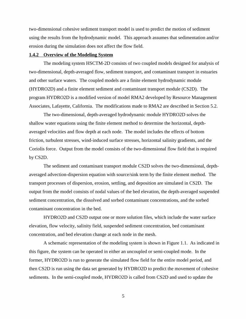
A schematic representation of the modeling system is shown in Figure 1.1. As indicated in
this figure, the system can be operated in either an uncoupled or semi-coupled mode. In the
former, HYDRO2D is run to generate the simulated flow field for the entire model period, and
then CS2D is run using the data set generated by HYDRO2D to predict the movement of cohesive
sediments. In the semi-coupled mode, HYDRO2D is called from CS2D and used to update the
5

flow field at each time step during model execution. This allows the changes in bed elevations and
the resulting changes in flow depths due to erosion and deposition to be incorporated into flow
field predictions at subsequent time steps.
The HSCTM-2D modeling system may be run using either a default option or a non-default
option. In the former, default values (contained in the program) for certain sediment-related input
parameters are used, whereas in the non-default mode all the input parameters have to be included
in the input data set. The default option of HSCTM-2D is discussed in Section 8.6. The purpose
of the default option is to allow model use even when all the required sediment-related parameters
(e.g., erosion/deposition rate coefficients) are not available. THE DEFAULT OPTION SHOULD
BE USED FOR QUALITATIVE ANALYSIS ONLY. The default option will allow the modeler
to make relative comparisons among various sites or designs.
A pre-processor and post-processor such as contained in the Surface Modeling System
(SMS) developed by the Engineering Graphics Laboratory at Bringham Young University will
save considerable time in generating and modifying the finite element grid of the system to be
modeled. SMS also generates the boundary condition file required by HYDRO2D, and reads in
the binary solutions files generated by HSCTM-2D for post-processing.
6
Figure 1.1 Flowchart of HSCTM-2D Modeling System
7

1.5 ORGANIZATION OF THE DOCUMENT
Section 2 provides information on availability of the program, and installation and run time
requirements. In Section 3 a brief description of estuarial hydrodynamics and a detailed
description of the mechanics of cohesive sediment transport are given. Section 4 includes a brief
introduction to the finite element method and the finite element formulation of the governing
equations for surface water flow and cohesive sediment transport. A detailed description of the
modeling system is given in Section 5. Section 6 discusses application of the modeling system
including limits for use, data collection and analysis, and model calibration. Section 7 has user
instructions and data input requirements, while Section 8 discusses data input requirements.
Section 9 describes two example problems. The Appendices include information about the
program such as flow charts of the program structure and subroutines, a laboratory sediment
testing program, and the data input manual for HYDRO2D.
8

SECTION 2
MODEL DEVELOPMENT, DISTRIBUTION ANDSUPPORT
The user should refer to the file READ.ME for the latest supplemental information, changes, and
or addendum to the HSCTM-2D model system and its related documentation. A copy of the
READ.ME file is distributed with the HSCTM-2D model package by the U.S. Environmental
Protection Agency (US EPA) Center for Exposure Assessment Modeling (CEAM). For the latest
information concerning the location, version number, and availability of the HSCTM-2D model
system, users should call the CEAM HelpDesk at 706/355-8400.
NOTE: The file READ.ME is an ASCII text (non-binary) file that can
be displayed on the monitor screen with the DOS TYPE command or
printed using the DOS PRINT command.
The READ.ME file contains the following information:
IntroductionAbstractDocumentationDistribution Diskette(s)File Name and ContentDevelopment SystemRoutine ExecutionRun Time and PerformanceMinimum File ConfigurationModificationTechnical Help ContactElectronic Support and DistributionDisclaimer
9
SECTION 3
THEORY
3.1 ESTUARIAL DYNAMICS
3.1.1 General Description
The hydrodynamic regime in an estuary is governed by the interaction among fresh water
flow, astronomical tides, surface (i.e., wind) stresses, wind-generated surface waves, the Coriolis
force, the geometry of the water body, and roughness characteristics of the sedimentary material
composing the bed (Dyer 1973). Fresh water flow and the next four factors mentioned are the
driving forces. Geometry includes the shape and bathymetry of the estuary. The geometry and bed
roughness interact with the driving forces to control the pattern of water motion (in particular the
shear stress and turbulence structure near the bed), frictional resistance, tidal damping, and degree
of tidal reflections (Ippen 1966).
The magnitude of tidal flow relative to fresh water inflow governs, to a large extent, the
intensity of vertical mixing of sea water with less dense fresh water. There exists in all estuaries a
longitudinal salinity profile that decreases from the mouth to the upper reaches of the estuary. The
existence of a longitudinal salinity gradient or baroclinic force implies that there could be a gravity
driven upstream transport of a high density sediment suspension in the lower portion of the water
column (Officer 1981; Mehta and Hayter 1981).
Winds affect the hydrodynamic regime and mixing in an estuary by generating surface
shear stress and waves. The surface stress is capable of generating a surface current (whose
magnitude will be approximately 3 percent of the wind speed at 9.1 m elevation (Hughes 1956))
and a super-elevation of the water surface along a land boundary located at the downwind end of
10
the estuary (Ippen 1966). The latter effect increases the degree of vertical mixing by causing a
vertical circulation cell with landward flow at the surface and seaward flow along the bottom.
Wave action, and in particular wave breaking, substantially increases the intensity of
turbulence and mixing in the upper portion of the water column. Along the banks and in shallow
areas, surface waves generated by the wind are capable of eroding bottom sediments. A tidal
current of sufficient strength to transport sediment eroded by other mechanisms is generally
present. Although the tidal current may not necessarily have enough force by itself to erode
sediment, it will cause suspended material to be advected and dispersed both longitudinally with
the main tidal flow and laterally by secondary currents towards the deeper sections of the estuary.
The Coriolis force, caused by the earth's rotation, has both a radial (horizontal) and a
tangential (vertical) component. The latter is generally negligible as it is linearly proportional to
and smaller than the vertical component of the flow velocity, which is typically an order of
magnitude smaller than the horizontal velocity components. The magnitude of the radial
component depends upon the size of the water body. Most extra-tropical estuaries are relatively
large and therefore the effect of this force on the hydrodynamic regime is measurable. Estuarial
hydrodynamics are described in detail elsewhere (Ippen 1966; Barnes and Green 1971; Dyer 1973;
Officer 1976; Fischer et al. 1979).
3.1.2 Governing Equations
3.1.2.1 Coordinate System
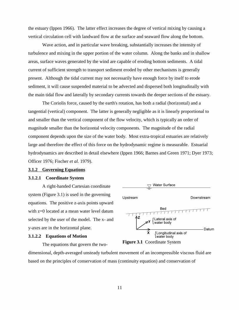
A right-handed Cartesian coordinate
system (Figure 3.1) is used in the governing
equations. The positive z-axis points upward
with z=0 located at a mean water level datum
selected by the user of the model. The x- and
y-axes are in the horizontal plane.
3.1.2.2 Equations of Motion
The equations that govern the two- Figure 3.1 Coordinate System
dimensional, depth-averaged unsteady turbulent movement of an incompressible viscous fluid are
based on the principles of conservation of mass (continuity equation) and conservation of
11
momentum (equations of motion). These equations are solved numerically in order to simulate the
velocity field in an estuary or other water body of interest.
3.1.2.2.1 Continuity -- The conservation of mass, as expressed by the continuity
equation, states that the mass of an incompressible fluid entering a control volume per unit time is
equal to the sum of the fluid mass leaving the control volume plus the change in volume of the
control volume. The depth-averaged continuity equation for an incompressible fluid is
M d M M% (u @ d) % (v @ d) ' 0 (3.1)
M t M x M y
where d = depth of flow, t = time, and u, v = depth-averaged water velocity components in the x-
and y-directions, respectively.
3.1.2.2.2 Conservation of Momentum -- The conservation of momentum for an
incompressible fluid states that the product of the fluid mass and acceleration is equal to the sum
of the body (gravitational) forces and the normal (pressure) and tangential (friction) surface forces
that act on the boundaries of the water body. The two-dimensional, depth-averaged equations of
motion for an incompressible viscous fluid are given by
M u M u M u M d M zb%u %v ' &g &g %S v
M t M x M y M x M x (3.2)
1 M% (dJ xx)%
M (dJ xy)%J
s &Jb
Dd M x M y x x
in the x-direction, and
M v M v M v M d M zb%u %v ' &g &g &Su
M t M x M y M y M y (3.3)
1 M M% d J % d J %Js
&Jb y yyx yyDd M x M y
in the y-direction, where g is the gravitational acceleration; zb is the bed elevation; D is the water
Js Jsdensity; S is the Coriolis parameter; and y are wind-induced shear stresses at the water surfacex
in the x- and y-directions, respectively; Jb and Jb are flow induced bed shear stresses in the xx y
12
x
and y-directions, respectively; and Jij (with i, j = x, y) is the depth-averaged turbulent shear stress
acting in the i-direction on a plane that is perpendicular to the j-direction.
Equations 3.1-3.3 are referred to as the shallow water equations and are applicable to
estuarial and other surface water flow problems in which the vertical (i.e., z) components of the
flow velocity and acceleration are small relative to the horizontal (i.e., x and y) components of the
flow velocity and acceleration. The three terms on the left hand side of equations 3.2 and 3.3
represent the substantive fluid acceleration in the x- and y-directions, respectively. The Coriolis
parameter S is equal to 2TsinN, where T is the angular velocity of the earth and N is the local
latitude. The terms Sv and -Su represent the Coriolis acceleration in the Northern Hemisphere in
the x- and y-directions, respectively. The surface wind shear stresses are given by
Js '
H W 2 cos R and Js
' H
W 2 sin R (3.4)x d y d
where H is an empirical wind shear coefficient; W is the wind speed; and R is the angle between
the positive x-axis and the wind direction. The depth-averaged turbulent shear stresses are
determined using Boussinesq's eddy viscosity model:
M uiJ ' gij for i, j ' x, y (3.5)ij M xi
in which xi, xj = x, y, and ui, uj = u, v; and gij is the eddy viscosity acting in the i-direction on a
plane that is perpendicular to the j-direction. Values of the eddy viscosities are dependent on both
fluid properties and the level of fluid turbulence.
The bottom shear stresses are given by two relationships:
' gu 2 % v 2 1/2 gv 2Jb u and Jb
' u % v 2 1/2 y (3.6)
C 2d C 2dz z
where Cz is the Chezy coefficient.
Substituting equations 3.4-3.6 into equations 3.2 and 3.3 gives the following form of the
depth-averaged equations of motion:
13
M u M u M u M d M zb%u %v ' &g &g %2vT sinN%
M t M x M y M x M x
(3.7)1 M Mu M Mu 2)1/2% %HW 2cosR&
gu (u 2%vgxxd
Mx gxyd
MyDd Mx My C 2dz
M v M v Mv M d M zb%u %v ' &g &g &2uT sinN%
M t M x My M y M y
(3.8)1 M Mv M Mv 2)1/2% %HW 2sinR&
gv (u 2%vgyxd
Mx gyyd
MyDd Mx My C 2dz
in the x- and y-directions, respectively. Equations 3.1, 3.7, and 3.8 are solved numerically using
the finite element method by the hydrodynamic module HYDRO2D.
3.2 COHESIVE SEDIMENT TRANSPORT
3.2.1 Description and Properties of Cohesive Sediments
3.2.1.1 Composition
Cohesive sediments consist primarily of terrigenous clay-sized particles composed of clay
and non-clay mineral components and organic material (Grim 1968). Clay particles are generally
less than 2 micrometers (µm) in size. As a result they are termed colloids and in water possess the
properties of plasticity, thixotropy and adsorption (van Olphen 1963). The most abundant types of
clay minerals are kaolinite, montmorillonite, illite, chlorite, vermiculite, and halloysite. The non-
clay minerals consist of, among others, quartz, carbonates, feldspar, and mica (Grim 1968). This
component of clay material is generally larger than 2 µm in size. The amount of non-clay minerals
present in a clay material currently cannot be determined with a high degree of accuracy.
The organic material often present in clay materials may be discrete particles of matter,
adsorbed organic molecules, or constituents inserted between clay layers (Grim 1968). Additional
possible components of clay materials are water-soluble salts, and adsorbed exchangeable ions and
contaminants.
14
3.2.1.2 Structure
Clay minerals are primarily hydrous aluminum silicates with magnesium or iron occupying
all or part of the aluminum positions in some clays, and with alkalines (e.g., sodium, potassium) or
alkaline earths (e.g., calcium, magnesium) also present in others (Grim 1968). Most clays are
composed of one or two atomic structural units or combinations of the two basic units.
Ions of one kind are sometimes substituted by ions of another kind with the same or
different valence. This process does not necessarily involve replacement. The tetrahedral and
octahedral cation distributions develop during initial formation of the mineral and not by later
substitution (Mitchell 1976). Substitution in all the clay materials, except for kaolinite, gives clay
particles a negative electric charge that is of great significance in coagulation of clays and in
adsorption of contaminants. Another cause of net particle charge is the preferential adsorption of
peptizing ions on the surface of the particle (van Olphen 1963).
3.2.1.3 Interparticle Forces
For particles in the colloidal size range, surface physicochemical forces exert a distinct
influence on the behavior of the particles due to the large specific area, i.e., ratio of surface area to
volume. As stated previously, most clay particles fall within the colloidal range in terms of both
their size (2 µm or less) and the controlling influence of surface forces on the behavior. In fact, the
average surface force on one clay particle is several orders of magnitude greater than the
gravitational force (Partheniades 1962).
The relationships between clay particles and water molecules are governed by interparticle
electrochemical forces. The different configurations and groupings as well as electric charges of
clay particles affect their association with water molecules (Grimshaw 1971).
Interparticle forces are both attractive and repulsive. The attractive forces present are the
London-van der Walls and are due to the nearly instantaneous fluctuation of the dipoles, which
result from the electrostatic attraction of the nucleus of one atom for the electron cloud of a
neighboring atom (Grimshaw 1971). These electrical attractive forces are weak and are only
significant when interacting atoms are very close together. The electrical attractive forces are
strong enough to cause structural build-up as they are additive between pairs of atoms. The
magnitude of these forces decreases with increasing temperature; they are only slightly dependent
on the salt concentration (i.e., salinity) of the medium (van Olphen 1963).
15
The repulsive forces of clay materials, which are due to negatively charged particle forces,
increase in an exponential fashion with decreasing particle separation. An increase in the salinity,
however, causes a decrease in the magnitude of the repulsive forces. This dependence on salinity
can best be explained using the concept of the electrical double layer and the surrounding diffuse
layer. van Olphen (1963) states that the double layer is composed of the net electrical charge of
the elementary clay particle and an equal quantity of ionic charge of opposite sign located in the
medium near the particle surface. The ions of opposite charge are called the counter-ions, i.e.,
cations. The counter-ion concentration increases with decreasing distance from the particle
surface. The layer of counter-ions is referred to as the diffuse layer. A clay particle and associated
double layer is referred to as a clay micelle (Partheniades 1971). When the salinity is increased,
the diffuse layer is compressed toward the particle surface (van Olphen 1963). The higher the
salinity, as well as the higher the valence of the cations that compose the diffuse layer, the more
this layer is compressed and the greater the repulsive force is decreased.
3.2.1.4 Cation Exchange Capacity
The cation exchange capacity (CEC) is an important property of clays by which they
adsorb certain cations and anions in exchange for those already present and retain them in an
exchangeable state. The CEC of different clays varies from 3 to 15 milliequivalents per 100 grams
(meq/100 gm) for kaolinite to 100 to 150 meq/100 gm for vermiculite. Higher CEC values
indicate greater capacity to adsorb other cations. The negative surface charge caused by
isomorphous substitution is neutralized by adsorbed cations located on the surfaces and edges of a
clay particle. These cations remain in an exchangeable position and may in turn be replaced by
other cations.
Two factors are the causes of cation exchange: (1) substitution within the lattice structure
results in unbalanced electrical charges in structural units of some clays, and (2) broken bonds
around the edges of tetrahedral-octahedral units give rise to unsatisfied charges. In both cases, the
unbalanced charges are balanced by adsorbed cations. The number of broken bonds and hence the
CEC increases with decreasing particle size.
The ability of particles to replace exchangeable cations depends on the concentration of the
replacing cation, the number of available exchange positions, and the nature of the ions in the
replacing solution. Increased concentration of the replacing cation results in greater cation
16

exchange. The release of an ion depends on the nature of the ion, the nature of the other ions
filling the remaining exchange positions, and the number of unfilled exchange sites. The higher
the valence of a cation, the greater is its replacing power and the more difficult it is to displace
when adsorbed on a clay. Some of the predominantly occurring cations in sediments are sodium,
potassium, calcium, aluminum, lead, copper, mercury, chromium, cadmium, and zinc.
3.2.2 Estuarial Cohesive Sediment Transport
3.2.2.1 Overview
In water with a very low salinity (less than about 1 part per thousand), the elementary
cohesive sediment particles are usually found in a dispersed state. Small amounts of salts,
however, are sufficient to repress the electrochemical surface repulsive forces among the
elementary particles, with the result that the particles coagulate to form flocs. A systematic "build
up" of flocs is defined as aggregation. An aggregate is the structural unit formed by the joining of
flocs. Each aggregate may contain thousands or even millions of elementary particles. The
transport properties of aggregates are affected by the hydrodynamic conditions and by the chemical
composition of the suspending fluid. Most estuaries contain abundant quantities of cohesive
sediments, which usually occur in the coagulated form in various degrees of aggregation.
Therefore, an understanding of the transport properties of these sediments in estuaries requires
knowledge of the manner in which aggregates are transported.
Cohesive sediment transport in estuaries is a complex process involving a strong coupling
among tides, baroclinic circulation, and the coagulated sediment. For an extensive description of
this process, the reader is referred to Postma (1967), Partheniades (1971), Barnes and Green
(1971), Krone (1972), Kirby and Parker (1977), Kranck (1980) and Dyer (1986). Figure 3.2 is a
schematic depiction. The case considered is one in which the estuary is stratified, and a stationary
saline wedge is formed. Various phases of suspended fine sediment transport are shown, assuming
a tidally averaged situation. In the case of a partially mixed estuary, the description will be
modified, but since relatively steep vertical density gradients are sometimes present even in such a
case, the sediment transport processes will generally remain qualitatively similar to that depicted.
[NOTE: HSCTM-2D is depth averaged and should not be applied to a stratified estuary. The
information in this section is provided for background information.]
17
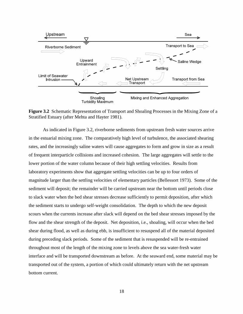
Figure 3.2 Schematic Representation of Transport and Shoaling Processes in the Mixing Zone of a Stratified Estuary (after Mehta and Hayter 1981).
As indicated in Figure 3.2, riverborne sediments from upstream fresh water sources arrive
in the estuarial mixing zone. The comparatively high level of turbulence, the associated shearing
rates, and the increasingly saline waters will cause aggregates to form and grow in size as a result
of frequent interparticle collisions and increased cohesion. The large aggregates will settle to the
lower portion of the water column because of their high settling velocities. Results from
laboratory experiments show that aggregate settling velocities can be up to four orders of
magnitude larger than the settling velocities of elementary particles (Bellessort 1973). Some of the
sediment will deposit; the remainder will be carried upstream near the bottom until periods close
to slack water when the bed shear stresses decrease sufficiently to permit deposition, after which
the sediment starts to undergo self-weight consolidation. The depth to which the new deposit
scours when the currents increase after slack will depend on the bed shear stresses imposed by the
flow and the shear strength of the deposit. Net deposition, i.e., shoaling, will occur when the bed
shear during flood, as well as during ebb, is insufficient to resuspend all of the material deposited
during preceding slack periods. Some of the sediment that is resuspended will be re-entrained
throughout most of the length of the mixing zone to levels above the sea water-fresh water
interface and will be transported downstream as before. At the seaward end, some material may be
transported out of the system, a portion of which could ultimately return with the net upstream
bottom current.
18

In the mixing zone of a typical estuary, the sediment transport rates often are an order of
magnitude greater than the rate of inflow of "new" sediment derived from upland or oceanic
sources. The estuarial sedimentary regime is characterized by several periodic (or quasi-periodic)
macro-time-scales, the most important of which are the tidal period (diurnal, semi-diurnal, or
mixed) and one-half the lunar month (spring-neap-spring cycle). The tidal period
is the most important since it is the fundamental period that characterizes the basic mode of
sediment transport in an estuary. The lunar month is often significant in determining net shoaling
rates.
From an Eulerian point of view, the superposition of oscillating tidal flows on the quasi-
steady state transport phenomenon depicted in Figure 3.2 results in corresponding oscillations of
the suspended sediment concentration with time as shown in Figure 3.3. Such a variation of the
suspended load ultimately results from a combination of advective and dispersive transport,
erosion, and deposition. Because of the complexity of the phenomenon, more than one
interpretation is possible as far as any schematic representation of these phenomena is concerned.
One such representation is shown in Figure 3.4. According to this description, cohesive sediments
can exist in four different physical states in an estuary: mobile suspension, stationary suspension,
partially consolidated bed, and settled bed. The last two are formed as a result of consolidation of
a stationary suspension. Stationary here implies little horizontal movement. A stationary
suspension, a partially consolidated bed and a settled bed may erode if the shear stress exceeds a
certain critical value. Erosion of a stationary suspension is referred to as redispersion or mass
erosion, whereas erosion of a partially consolidated bed or a settled bed is termed either
resuspension or surface erosion.
To summarize, the sedimentary regime in an estuary is controlled by the hydrodynamics,
chemical composition of the fluid, and physicochemical properties of the cohesive sediments.
These factors affect the processes of erosion, advection, dispersion, aggregation, settling,
deposition, and consolidation. A description of these processes follows that of cohesive sediment
beds.
3.2.2.2 Sediment Bed
A flow-deposited bed of cohesive sediment aggregates possesses a vertical density and
shear (i.e., yield) strength profile. The profile changes in time primarily due to consolidation and
19
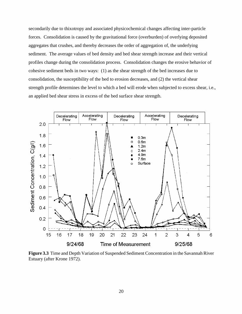
secondarily due to thixotropy and associated physicochemical changes affecting inter-particle
forces. Consolidation is caused by the gravitational force (overburden) of overlying deposited
aggregates that crushes, and thereby decreases the order of aggregation of, the underlying
sediment. The average values of bed density and bed shear strength increase and their vertical
profiles change during the consolidation process. Consolidation changes the erosive behavior of
cohesive sediment beds in two ways: (1) as the shear strength of the bed increases due to
consolidation, the susceptibility of the bed to erosion decreases, and (2) the vertical shear
strength profile determines the level to which a bed will erode when subjected to excess shear, i.e.,
an applied bed shear stress in excess of the bed surface shear strength.
Figure 3.3 Time and Depth Variation of Suspended Sediment Concentration in the Savannah River Estuary (after Krone 1972).
20
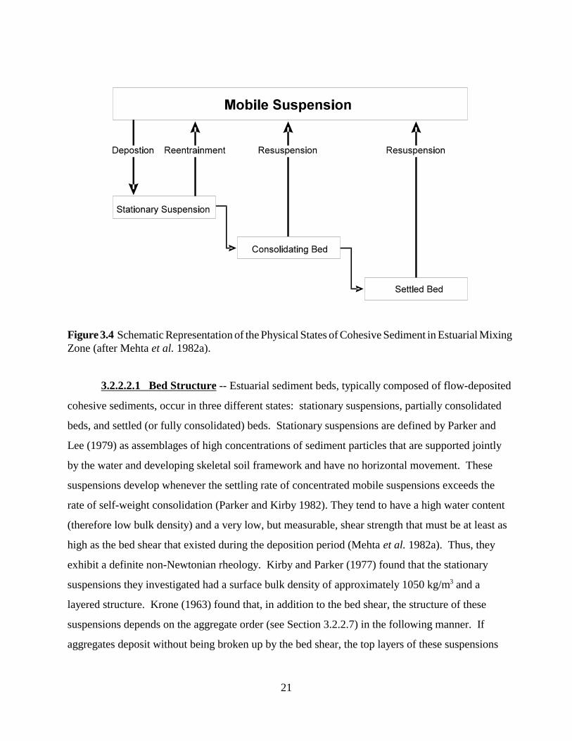
Figure 3.4 Schematic Representation of the Physical States of Cohesive Sediment in Estuarial Mixing Zone (after Mehta et al. 1982a).
3.2.2.2.1 Bed Structure -- Estuarial sediment beds, typically composed of flow-deposited
cohesive sediments, occur in three different states: stationary suspensions, partially consolidated
beds, and settled (or fully consolidated) beds. Stationary suspensions are defined by Parker and
Lee (1979) as assemblages of high concentrations of sediment particles that are supported jointly
by the water and developing skeletal soil framework and have no horizontal movement. These
suspensions develop whenever the settling rate of concentrated mobile suspensions exceeds the
rate of self-weight consolidation (Parker and Kirby 1982). They tend to have a high water content
(therefore low bulk density) and a very low, but measurable, shear strength that must be at least as
high as the bed shear that existed during the deposition period (Mehta et al. 1982a). Thus, they
exhibit a definite non-Newtonian rheology. Kirby and Parker (1977) found that the stationary
suspensions they investigated had a surface bulk density of approximately 1050 kg/m3 and a
layered structure. Krone (1963) found that, in addition to the bed shear, the structure of these
suspensions depends on the aggregate order (see Section 3.2.2.7) in the following manner. If
aggregates deposit without being broken up by the bed shear, the top layers of these suspensions
21
will be composed of an aggregate network whose aggregation order is one higher than that of the
individual settling aggregates; therefore, these layers will have lower bulk densities and shear
strengths than those of the aggregates that form them.
Whether redispersion of these suspensions occurs during periods of erosion depends upon
the mechanical shear strength of this aggregate network. That portion remaining on the bed
undergoes: (1) self-weight consolidation, and (2) thixotropic effects, defined as the slow
rearrangement of deposited aggregates attributed to internal energy and unbalanced internal
stresses (Mitchell 1961), both of which reduce the order of aggregation of sub-surface bed layers.
This implies that the bed becomes stratified with respect to density and shear strength, with both
properties typically increasing monotonically with depth, at least under laboratory conditions
(Mehta et al. 1982a).
Continued consolidation eventually results in the formation of settled mud, defined by
Parker and Lee (1979) as "assemblages of particles predominantly supported by the effective
contact stresses between particles as well as any excess pore water pressure." This portion of the
bed has a lower water content, lower order of aggregation, and higher shear strength. The settled
mud in the Severn Estuary and Inner Bristol Channel, United Kingdom, was found to posses a
bulk density ranging from 1300 to 1700 kg/m3 (Kirby and Parker 1983).
The nature of the density and shear strength profiles typically found in flow-deposited
cohesive sediment beds has been revealed in laboratory tests by, among others, Richards et al.
(1974), Owen (1975), Thorn and Parsons (1980), Parchure (1980), Bain (1981), Dixit (1982), and
Burt and Parker (1984). A review of this subject is given by Hayter (1983).
3.2.2.2.2 Effect of Salinity on Bed Structure -- For most cohesive soils the inter-particle
and inter-floc contact is considered to be the only significant region between particles where
normal stresses and shear stresses can be transmitted (Mitchell et al. 1969). In particular, it seems
very likely that the primary role of the double-layer interaction and other physicochemical forces is
to control the structure of the soil and to alter the transmitted stresses from what they would be due
to the flow-induced shear and overburden normal stresses alone. Hayter and Mehta (1982) discuss
the effect of swelling and permeability (including the effect of salinity) on the structure of a
cohesive soil. They also discuss the effect of the salinity of the pore fluids on bed density.
22
Using the method described by Mehta et al. (1982a), the bed shear strength, J , of mudc
from Lake Francis, Nebraska, as a function of depth below the initial bed surface, Z, was
determined as a function of salinity for salinities from 0 to 10 ppt (Figure 3.5). This mud, of
which 50% was finer than 2µm (clay-sized particles), with montmorillonite, illite, kaolinite and
quartz being the predominant minerals, had a CEC of 100 meq/100 g. Two trends are observed in
this graph. First, Jc increases with depth in the upper part of the bed for all salinities (no definite
data could be obtained for the lower part of the bed, i.e., for Z > 0.5 cm, inasmuch as this portion
of the bed did not erode during these experiments). Second, Jc increases with increasing salinity
from 0 to 2 ppt; thereafter, for salinities up to 10 ppt, no measurable increase in J occurred.c
3.2.2.3 Erosion
Erosion of cohesive soils occurs whenever the shear stress induced by fluid flow over the
bed is great enough to break the electrochemical interparticle bonds (Partheniades 1965; Paaswell
1973). When this happens, erosion takes place by the removal of individual sediment
particles and/or aggregates. This type of erosion is time dependent and is defined as surface
erosion or resuspension. In contrast, another type of erosion occurs more or less instantaneously
by the removal or entrainment of relatively large pieces of soil. This process is referred to as mass
erosion or redispersion occurs when the flow induced shear stresses on the bed exceed the soil
bulk strength along some deep seated plane.
A number of laboratory investigations were carried out in the 1960's and 1970's in order to
determine the rate of resuspension, g, defined as the mass of sediment eroded per unit bed surface
area per unit time as a function of bed shear in steady, turbulent flows. An important conclusion
from these tests was that the usual soil indices such as liquid and plastic limit do not adequately
describe the erosive behavior of these soils (Mehta 1981). For example, Partheniades (1962)
concluded that the bed shear strength as measured by standard tests, e.g., the direct-shear test
(Terzaghi and Peck 1960), has no direct relationship with the soil's resistance to erosion, which is
essentially governed by the strength of the interparticle and interaggregate bonds. Shown in Table
3.1 are various physicochemical factors known to govern the erosive properties of cohesive soils.
These factors must be specified to properly characterize the erosive behavior. The hydrodynamic
factors define the erosive forces; the bed and fluid physicochemical properties determine the
resistivity of the bed to erosion.
23
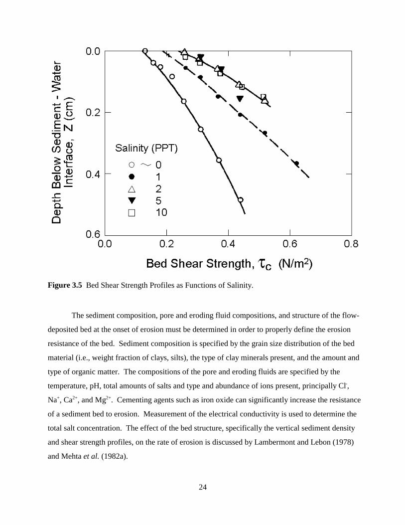
Figure 3.5 Bed Shear Strength Profiles as Functions of Salinity.
The sediment composition, pore and eroding fluid compositions, and structure of the flow-
deposited bed at the onset of erosion must be determined in order to properly define the erosion
resistance of the bed. Sediment composition is specified by the grain size distribution of the bed
material (i.e., weight fraction of clays, silts), the type of clay minerals present, and the amount and
type of organic matter. The compositions of the pore and eroding fluids are specified by the -temperature, pH, total amounts of salts and type and abundance of ions present, principally Cl ,
Na+, Ca2+, and Mg2+. Cementing agents such as iron oxide can significantly increase the resistance
of a sediment bed to erosion. Measurement of the electrical conductivity is used to determine the
total salt concentration. The effect of the bed structure, specifically the vertical sediment density
and shear strength profiles, on the rate of erosion is discussed by Lambermont and Lebon (1978)
and Mehta et al. (1982a).
24

Table 3.1 Principal Factors Controlling Erosion of Saturated Cohesive Sediment Beds
HYDRODYNAMIC FACTORS (Erosive Force)
BED SHEAR STRESS Flow Characteristics
Bed-Fluid Interface
BED AND FLUID PROPERTIES (Resistive Force)
PROPERTY FACTOR INDICATOR
SEDIMENT COMPOSITION
Clay Mineral Type Ion Exchange Capacity
Clay Percentage by Weight
Organic Matter
PORE FLUID COMPOSITION
Mono- and Di-valent Cation Concentrations
Conductivity (Na+, Ca2+, Mg2+)
Relative Abundance of Mono- and Divalent Cations
SAR
Temperature
pH
ERODING FLUID COMPOSITION
Salinity (NaCl, CaCl2, MgCl2)
Temperature
pH
Cementing Agents (Iron Oxide, etc.)
BED STRUCTURE Stress History Placed Bed
Deposited Bed
25
The erosive forces, characterized by the flow-induced instantaneous bed shear stress, are
determined by the flow characteristics and the surface roughness of the fluid-bed interface.
Several different types of relationships between the rate of erosion, g, and the time-mean value of
the flow-induced bed shear stress, Jb, have been reported for non-stratified beds. These include
statistical-mechanical models (Partheniades 1965; Christensen 1965), a rate process model
(Paaswell 1973; Kelley and Gularte 1981), and empirical relationships (Ariathurai and
Arulanandan 1978).
The resuspension rate, g, is related to the time-rate of change of the suspension
concentration, dC/dt, and to the time-rate of change of the depth of erosion, ze, with respect to the
original bed surface elevation by two expressions:
dC e dC g ' d ; dC ' 1 D (ze )
dz ' / (3.9)
dt d t d s d t d t 00 e
where:
Ds(ze) is the dry sediment density at the elevation corresponding to ze,
C = mass of sediment per unit volume of waster and sediment mixture.
Ariathurai and Arulanandan (1978) found the following general relationship for
consolidated beds:
Jb & J cg ' M' (3.10)J c
where M' = M"Jc, where M is termed the erodibility constant, Jb is the flow induced bed shear
stress and Jc is the bed shear strength.
Figure 3.6 shows the measured variation of C with time typically found by several
investigators (Partheniades 1962; Mehta and Partheniades 1979; Mehta et al. 1982a) in laboratory
resuspension tests with flow-deposited (stratified) beds under a constant Jb. As observed, dC/dt is
high initially, decreases monotonically with time, and appears to approach zero. The value of J at
the depth of erosion at which dC/dt, and therefore g becomes essentially zero has been interpreted
to be equal to Jb (Mehta et al. 1982a). This interpretation is based on the hypothesis that erosion
continues as long as Jb > J . Erosion is arrested at the bed level at which Jb - J = 0. Thisc c
interpretation, coupled with measurement of Ds(zb) and the variation of C with time results in an
26
c
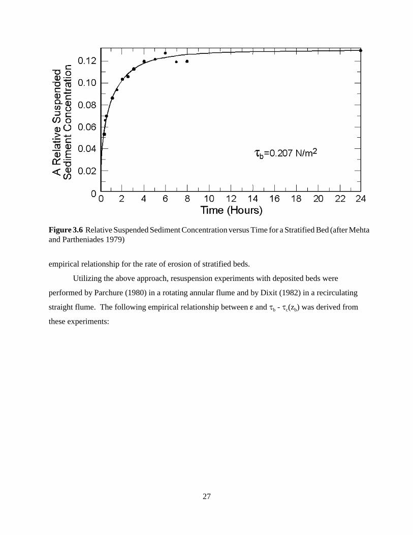
Figure 3.6 Relative Suspended Sediment Concentration versus Time for a Stratified Bed (after Mehta and Partheniades 1979)
empirical relationship for the rate of erosion of stratified beds.
Utilizing the above approach, resuspension experiments with deposited beds were
performed by Parchure (1980) in a rotating annular flume and by Dixit (1982) in a recirculating
straight flume. The following empirical relationship between g and Jb - Jc(zb) was derived from
these experiments:
27
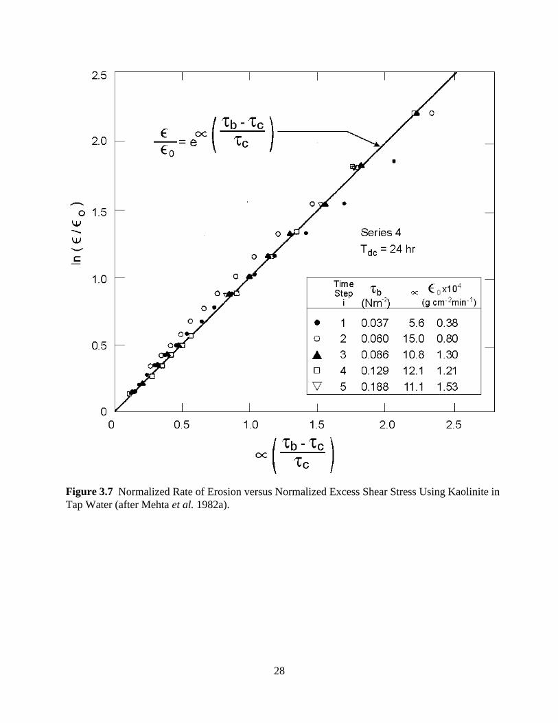
Figure 3.7 Normalized Rate of Erosion versus Normalized Excess Shear Stress Using Kaolinite in Tap Water (after Mehta et al. 1982a).
28
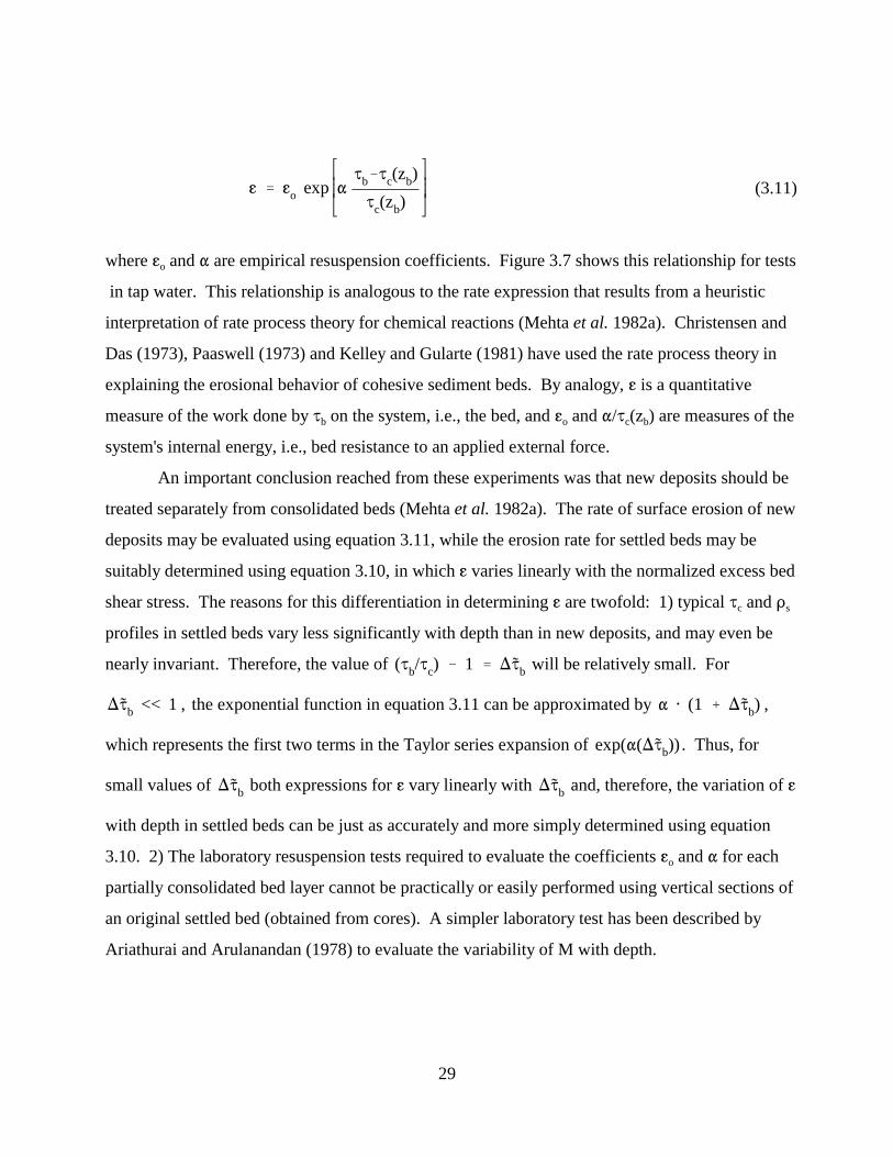
Jb&J (zb)cg ' go exp " (3.11)J (zb)c
where go and " are empirical resuspension coefficients. Figure 3.7 shows this relationship for tests
in tap water. This relationship is analogous to the rate expression that results from a heuristic
interpretation of rate process theory for chemical reactions (Mehta et al. 1982a). Christensen and
Das (1973), Paaswell (1973) and Kelley and Gularte (1981) have used the rate process theory in
explaining the erosional behavior of cohesive sediment beds. By analogy, g is a quantitative
measure of the work done by Jb on the system, i.e., the bed, and go and "/Jc(zb) are measures of the
system's internal energy, i.e., bed resistance to an applied external force.
An important conclusion reached from these experiments was that new deposits should be
treated separately from consolidated beds (Mehta et al. 1982a). The rate of surface erosion of new
deposits may be evaluated using equation 3.11, while the erosion rate for settled beds may be
suitably determined using equation 3.10, in which g varies linearly with the normalized excess bed
shear stress. The reasons for this differentiation in determining g are twofold: 1) typical J and Dc s
profiles in settled beds vary less significantly with depth than in new deposits, and may even be
nearly invariant. Therefore, the value of (Jb/J ) & 1 ' )Jb will be relatively small. For c
)Jb << 1 , the exponential function in equation 3.11 can be approximated by " @ (1 % )Jb) ,
which represents the first two terms in the Taylor series expansion of exp("()Jb)) . Thus, for
small values of )Jb both expressions for g vary linearly with )Jb and, therefore, the variation of g
with depth in settled beds can be just as accurately and more simply determined using equation
3.10. 2) The laboratory resuspension tests required to evaluate the coefficients go and " for each
partially consolidated bed layer cannot be practically or easily performed using vertical sections of
an original settled bed (obtained from cores). A simpler laboratory test has been described by
Ariathurai and Arulanandan (1978) to evaluate the variability of M with depth.
29
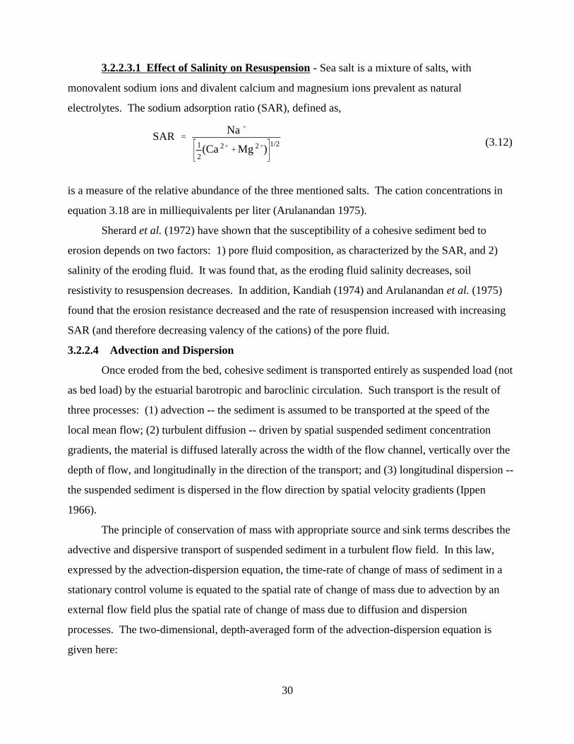
3.2.2.3.1 Effect of Salinity on Resuspension - Sea salt is a mixture of salts, with
monovalent sodium ions and divalent calcium and magnesium ions prevalent as natural
electrolytes. The sodium adsorption ratio (SAR), defined as,
Na %
SAR ' 1 (Ca 2%%Mg 2%) 1/2 (3.12) 2
is a measure of the relative abundance of the three mentioned salts. The cation concentrations in
equation 3.18 are in milliequivalents per liter (Arulanandan 1975).
Sherard et al. (1972) have shown that the susceptibility of a cohesive sediment bed to
erosion depends on two factors: 1) pore fluid composition, as characterized by the SAR, and 2)
salinity of the eroding fluid. It was found that, as the eroding fluid salinity decreases, soil
resistivity to resuspension decreases. In addition, Kandiah (1974) and Arulanandan et al. (1975)
found that the erosion resistance decreased and the rate of resuspension increased with increasing
SAR (and therefore decreasing valency of the cations) of the pore fluid.
3.2.2.4 Advection and Dispersion
Once eroded from the bed, cohesive sediment is transported entirely as suspended load (not
as bed load) by the estuarial barotropic and baroclinic circulation. Such transport is the result of
three processes: (1) advection -- the sediment is assumed to be transported at the speed of the
local mean flow; (2) turbulent diffusion -- driven by spatial suspended sediment concentration
gradients, the material is diffused laterally across the width of the flow channel, vertically over the
depth of flow, and longitudinally in the direction of the transport; and (3) longitudinal dispersion -
the suspended sediment is dispersed in the flow direction by spatial velocity gradients (Ippen
1966).
The principle of conservation of mass with appropriate source and sink terms describes the
advective and dispersive transport of suspended sediment in a turbulent flow field. In this law,
expressed by the advection-dispersion equation, the time-rate of change of mass of sediment in a
stationary control volume is equated to the spatial rate of change of mass due to advection by an
external flow field plus the spatial rate of change of mass due to diffusion and dispersion
processes. The two-dimensional, depth-averaged form of the advection-dispersion equation is
given here:
30
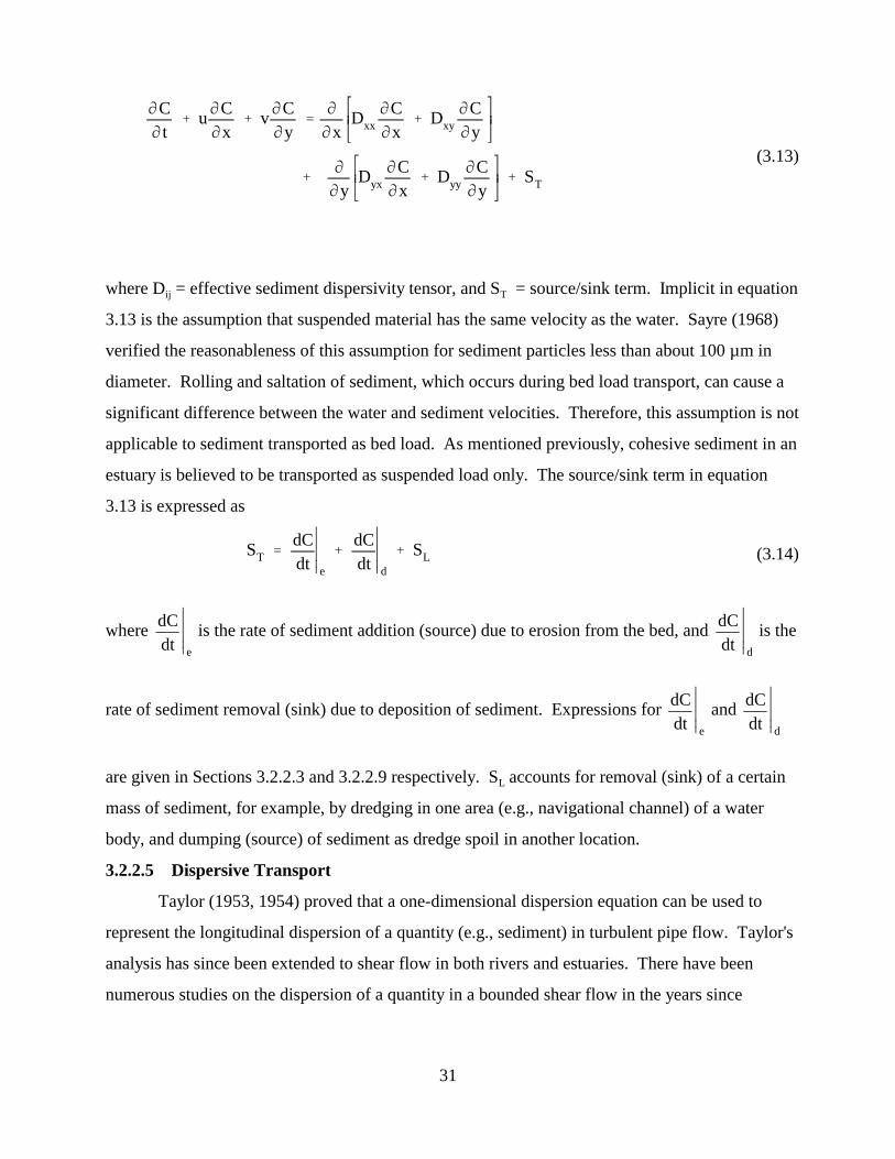
M C M C M C '
M M C M C% u % v D % D xx xyM t M x M y M x M x M y
(3.13)M M C M C
% D % D % STyx yyM y M x M y
where Dij = effective sediment dispersivity tensor, and ST = source/sink term. Implicit in equation
3.13 is the assumption that suspended material has the same velocity as the water. Sayre (1968)
verified the reasonableness of this assumption for sediment particles less than about 100 µm in
diameter. Rolling and saltation of sediment, which occurs during bed load transport, can cause a
significant difference between the water and sediment velocities. Therefore, this assumption is not
applicable to sediment transported as bed load. As mentioned previously, cohesive sediment in an
estuary is believed to be transported as suspended load only. The source/sink term in equation
3.13 is expressed as
dC dCST ' / %
dt 00/ d
% SL (3.14)dt 00 e
dC dCwhere / is the rate of sediment addition (source) due to erosion from the bed, and dt 00/ d
is the dt 00 e
dC dCrate of sediment removal (sink) due to deposition of sediment. Expressions for / and dt / ddt 00 e
are given in Sections 3.2.2.3 and 3.2.2.9 respectively. SL accounts for removal (sink) of a certain
mass of sediment, for example, by dredging in one area (e.g., navigational channel) of a water
body, and dumping (source) of sediment as dredge spoil in another location.
3.2.2.5 Dispersive Transport
Taylor (1953, 1954) proved that a one-dimensional dispersion equation can be used to
represent the longitudinal dispersion of a quantity (e.g., sediment) in turbulent pipe flow. Taylor's
analysis has since been extended to shear flow in both rivers and estuaries. There have been
numerous studies on the dispersion of a quantity in a bounded shear flow in the years since
31
0 0
Taylor's work. In this section, a brief review of dispersive transport theory precedes that of
estuarial dispersion.
The governing equation (eq. 3.13) derived for the two-dimensional, depth-averaged
transport of suspended sediment in a turbulent flow field includes dispersive transport terms that
account for transport of sediment by processes other than advective transport. Some of these
processes include the effects of spatial (i.e., transverse and vertical) velocity variations in bounded
shear flows and turbulent diffusion. Thus, the effective sediment dispersion coefficients in
equation 3.13 must include the effect of all processes whose scale is less than the grid size of the
model, or, in other words, what has been averaged over time and/or space (Fischer et al. 1979).
For example, the effect of the vertical concentration gradient would have to be (at least
approximately) incorporated in the dispersion coefficients in depth-averaged transport models.
Diffusion is defined as "the transport in a given direction at a point in the flow due to the
difference between the true advection in that direction and the time average of the advection in that
direction," and dispersion is defined as "the transport in a given direction due to the difference
between the true advection in that direction and the spatial average of the advection in that
direction" (Holley 1969). Holley delineates the fact that diffusion and dispersion are both actually
advective transport mechanisms, and that in a given flow field, the relative importance of one
mechanism over the other depends on the magnitude of the concentration gradient. In equation
3.13, the effective sediment dispersion coefficients are equal to the sum of the turbulent diffusion
and dispersion coefficients. This approach follows the analysis of Aris (1956) that showed that the
coefficients due to turbulent diffusion and shear flow (dispersion) were additive. Thus, the
analytic expressions to be used for the effective sediment dispersion tensor would include, at least
in some sense, both diffusion and dispersion.
Fischer (1966) showed that the dispersion of a given quantity of tracer injected into a
natural stream is divided into two separate phases. The first is the convective period in which the
tracer mixes vertically, laterally, and longitudinally until it is completely distributed across the
stream. The second phase is the diffusive period during which the lateral and possibly the vertical
(depending on the nature of the tracer) concentration gradient is small, and the longitudinal
concentration profile is highly skewed. Equation 3.13 is strictly valid only in the diffusive period.
The criterion for determining whether the dispersing tracer is in the diffusive period is if it has
32
been in the flow longer than the Lagrangian time scale and has spread over a distance wider than
the Lagrangian length scale (Fischer et al. 1979). The latter scale is a measure of the distance a
particle travels before it forgets its initial conditions (i.e., initial position and velocity).
Analytic expressions for the sediment (mass) diffusion coefficients can be obtained by
analogy with the kinematic eddy viscosity. Specifically, the Reynolds analogy assumes that the
processes of momentum and mass transfer are similar, and that the turbulent diffusion coefficient,
and the kinematic eddy viscosity, gv, are in fact linearly proportional. Jobson and Sayre (1970)
verified the Reynolds analogy for sediment particles in the Stokes range (less than about 100 µm
in diameter). They found that the "portion of the turbulent mass transfer coefficient for sediment
particles which is directly attributable to tangential components of turbulent velocity fluctuations:
(a) is approximately proportional to the momentum transfer coefficient and the proportionality
constant is less than or equal to 1; and (b) decreases with increasing particle size." Therefore, the
effective sediment mass dispersion coefficients for cohesive sediments may be justifiably assumed
to be equal to those for the water itself.
Fischer et al. (1979) define four primary mechanisms of dispersion in estuaries:
1) gravitational circulation, 2) shear-flow dispersion, 3) bathymetry-induced dispersion and
4) wind-induced circulations. Gravitational or baroclinic circulation in estuaries is the flow
induced by the density difference between fresh water at the landward end and sea water at the
ocean end. There are two types of gravitational circulation. Transverse gravitational circulation is
depth-averaged flow that is predominantly seaward in the shallow regions of a cross-section and
landward in the deeper parts. Figure 3.8 depicts this net depth-averaged upstream (landward) and
downstream (seaward) transport and the resulting transverse flow from the deeper to shallower
parts of the cross-section. The interaction between the cross-sectional bathymetry and baroclinic
flow causes the transverse circulation. Vertical gravitational circulation is schematically
illustrated in Figure 3.8, which shows the predominantly seaward flow in the upper part of the
flow and landward flow in the lower part. Fischer (1972) believed that vertical gravitational
circulation is more important than transverse circulation only in highly stratified estuaries.
The mechanism of shear-flow dispersion is thought to be the dominant mechanism in long,
fairly uniform sections of well-mixed and partially stratified estuaries (Fischer et al. 1979). Holley
et al. (1970) applied the dispersion analysis of Taylor (1954) to oscillating flow in estuaries. They
33
concluded that, for wide estuaries, the effect of the vertical velocity distribution on shear-flow
dispersion is dominant over that of the transverse velocity distribution. The exact opposite
situation was found for relatively narrow estuaries.
The joint influence of bathymetry and density differences on dispersion has already been
mentioned in reference to baroclinic circulation. Other examples of bathymetry-induced
dispersion include: intrusion of salinity or sediment in certain parts of a cross-section caused by
channelization of flood and ebb tides in tidal inlets or narrow estuaries (Fischer et al. 1979) and
enhanced dispersion of a quantity (e.g., pollutant) or intrusion of salinity in tidal flats and side
embayments, which serve as storage areas for these constituents, caused by the out of phase flow
that occurs between the main channel and such features (Okubo 1973).
An example of wind-induced circulation is shown in Figure 3.9. The steady onshore wind
causes a circulation in the wind direction in the shallow bay, where the smaller water mass per unit
surface area results in a higher acceleration and therefore quicker response to wind-induced surface
stresses, and in the opposite direction in deeper sections of the channel. Such a circulation can
cause significant dispersion (Fischer et al. 1979).
3.2.2.6 Coagulation
Coagulation of suspended cohesive sediments depends upon interparticle collision and
cohesion. Cohesion and collision, discussed in detail elsewhere (Kruyt (1952), Einstein and Krone
(1962), Krone (1962), Partheniades (1964), O'Melia (1972), and Hunt (1980)) are briefly reviewed
here.
The collision frequency, FC, for suspended sediment particles of effective diameters di and
dj is given by (Hunt 1980):
FC ' $(di,dj) dNi dNj (3.15)
where $(di,dj) = collision function determined by the collision mechanism (discussed below),
dNi= number of particles with sizes between di and di + )(di) per unit volume of the fluid and dNj=
number of particles with sizes between dj and dj + )(dj) per unit volume of the fluid.
There are three principle mechanisms of interparticle collision in suspension, and these
influence the rate at which elementary sediment particles coagulate. The first is due to Brownian
motion resulting from thermal motions of molecules of the suspending ambient medium. The
collision function corresponding to this mechanism is given by (Hunt 1980):
34

$b(di,d ) ' 2 kTk (di % dj )2
(3.16)j 3 µ di dj
where k = Boltzmann constant, Tk = absolute temperature and µ = dynamic viscosity of the fluid.
Generally, coagulation rates by this mechanism are too slow to be significant in estuaries unless
the suspended sediment concentration exceeds 10 g/l as it sometimes does in fluid mud (a high
density near-bed layer). Aggregates formed by this mechanism are weak, with a lace-like
structure, and are easily fractured by shearing, especially in the high shear environment near the
bed, or are crushed easily when deposited (Krone 1962).
R
The second mechanism is due to internal shearing produced by local velocity gradients in
the fluid. Collision will occur if the paths of the particles' centers in the velocity gradient are
displaced by a distance that is less than the sum of their radii (referred to as the collision radius,
ij, between di and dj size particles). The collision function is given as
G R 3$sh (di,dj) '
6 i j (3.17)
where G is the local shearing rate and Rij = di + dj. Aggregates produced by this mechanism tend
to be spherical, and are relatively dense and strong because only those bonds that are strong
enough to resist the internal shearing due to local velocity gradients can survive.
The third mechanism, differential sedimentation, results from particles of different sizes
having different settling velocities. A larger particle, due to its higher settling velocity, will collide
with smaller, more slowly settling particles and will have a tendency to "pick up" these particles.
The collision function is expressed as
Df & D $ds (di,dj) ' Bg (di % d )2 / di
2 & dj
2 / (3.18)j72 < D
where < = kinematic viscosity of the fluid, Df = floc density and D = fluid density. This mechanism
produces relatively weak aggregates and contributes to the often observed rapid clarification of
estuarial waters at slack.
35
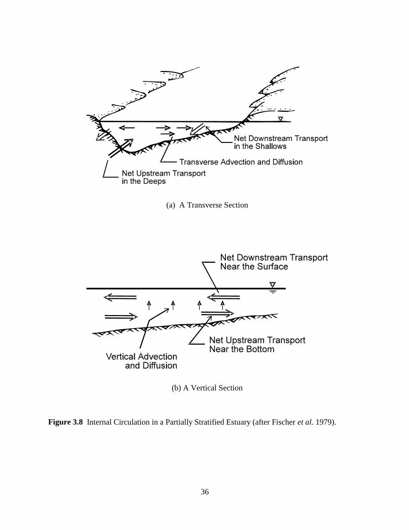
(a) A Transverse Section
(b) A Vertical Section
Figure 3.8 Internal Circulation in a Partially Stratified Estuary (after Fischer et al. 1979).
36
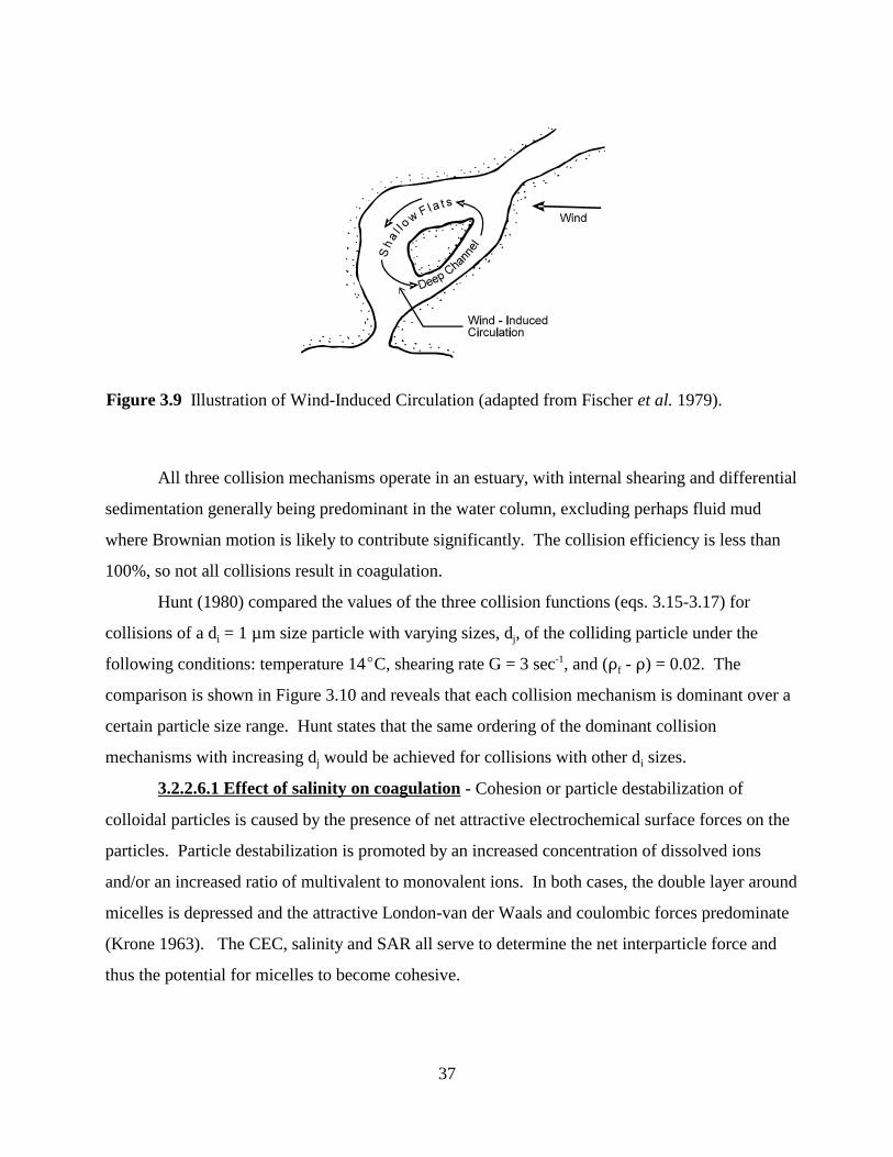
Figure 3.9 Illustration of Wind-Induced Circulation (adapted from Fischer et al. 1979).
All three collision mechanisms operate in an estuary, with internal shearing and differential
sedimentation generally being predominant in the water column, excluding perhaps fluid mud
where Brownian motion is likely to contribute significantly. The collision efficiency is less than
100%, so not all collisions result in coagulation.
Hunt (1980) compared the values of the three collision functions (eqs. 3.15-3.17) for
collisions of a di = 1 µm size particle with varying sizes, dj, of the colliding particle under the
following conditions: temperature 14EC, shearing rate G = 3 sec-1, and (Df - D) = 0.02. The
comparison is shown in Figure 3.10 and reveals that each collision mechanism is dominant over a
certain particle size range. Hunt states that the same ordering of the dominant collision
mechanisms with increasing dj would be achieved for collisions with other di sizes.
3.2.2.6.1 Effect of salinity on coagulation - Cohesion or particle destabilization of
colloidal particles is caused by the presence of net attractive electrochemical surface forces on the
particles. Particle destabilization is promoted by an increased concentration of dissolved ions
and/or an increased ratio of multivalent to monovalent ions. In both cases, the double layer around
micelles is depressed and the attractive London-van der Waals and coulombic forces predominate
(Krone 1963). The CEC, salinity and SAR all serve to determine the net interparticle force and
thus the potential for micelles to become cohesive.
37
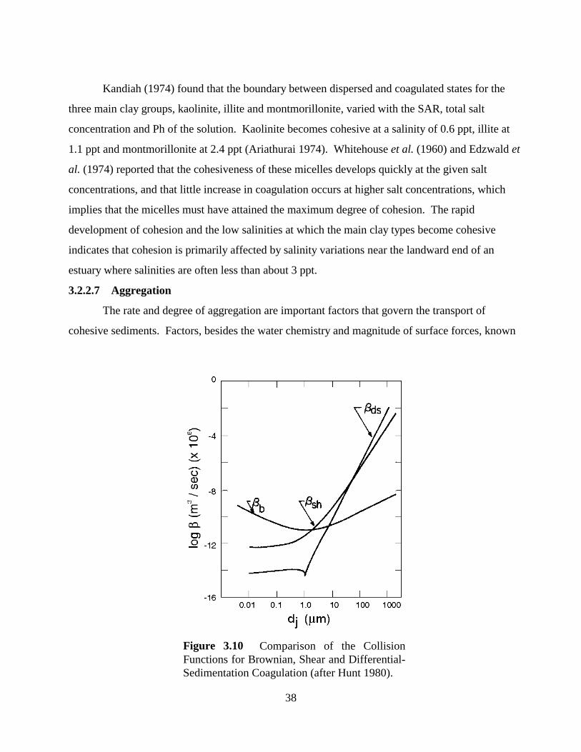
Kandiah (1974) found that the boundary between dispersed and coagulated states for the
three main clay groups, kaolinite, illite and montmorillonite, varied with the SAR, total salt
concentration and Ph of the solution. Kaolinite becomes cohesive at a salinity of 0.6 ppt, illite at
1.1 ppt and montmorillonite at 2.4 ppt (Ariathurai 1974). Whitehouse et al. (1960) and Edzwald et
al. (1974) reported that the cohesiveness of these micelles develops quickly at the given salt
concentrations, and that little increase in coagulation occurs at higher salt concentrations, which
implies that the micelles must have attained the maximum degree of cohesion. The rapid
development of cohesion and the low salinities at which the main clay types become cohesive
indicates that cohesion is primarily affected by salinity variations near the landward end of an
estuary where salinities are often less than about 3 ppt.
3.2.2.7 Aggregation
The rate and degree of aggregation are important factors that govern the transport of
cohesive sediments. Factors, besides the water chemistry and magnitude of surface forces, known
Figure 3.10 Comparison of the Collision Functions for Brownian, Shear and Differential-Sedimentation Coagulation (after Hunt 1980).
38
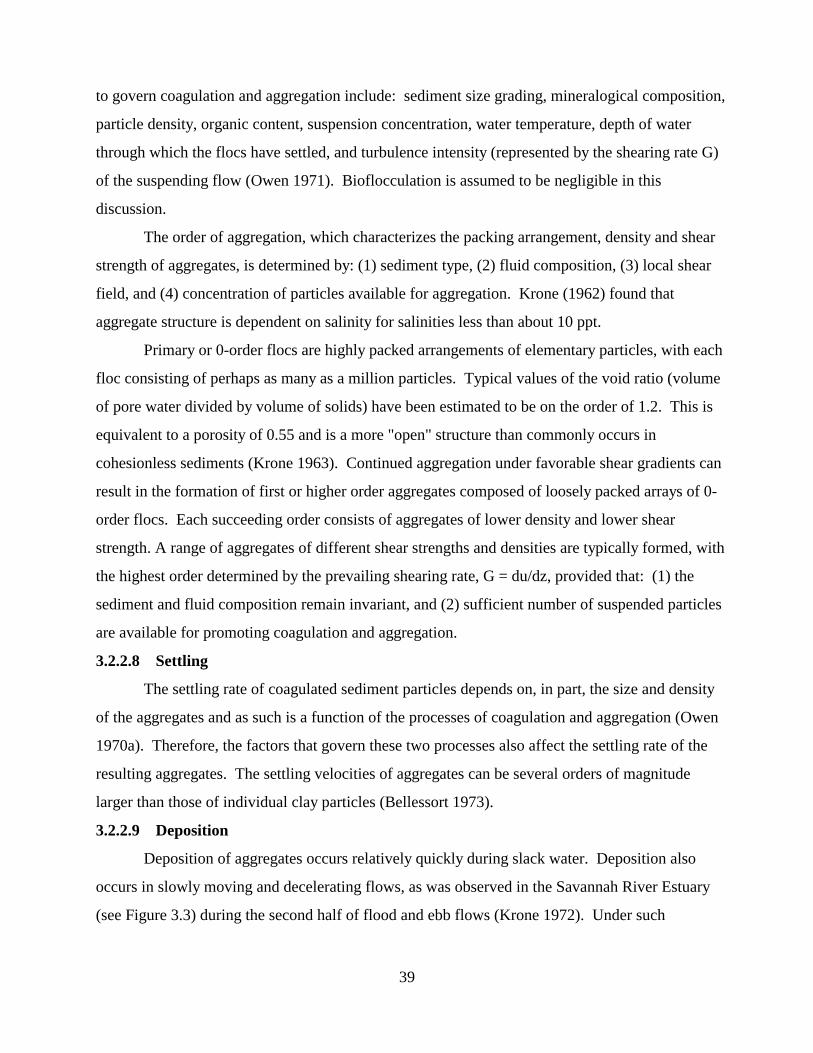
to govern coagulation and aggregation include: sediment size grading, mineralogical composition,
particle density, organic content, suspension concentration, water temperature, depth of water
through which the flocs have settled, and turbulence intensity (represented by the shearing rate G)
of the suspending flow (Owen 1971). Bioflocculation is assumed to be negligible in this
discussion.
The order of aggregation, which characterizes the packing arrangement, density and shear
strength of aggregates, is determined by: (1) sediment type, (2) fluid composition, (3) local shear
field, and (4) concentration of particles available for aggregation. Krone (1962) found that
aggregate structure is dependent on salinity for salinities less than about 10 ppt.
Primary or 0-order flocs are highly packed arrangements of elementary particles, with each
floc consisting of perhaps as many as a million particles. Typical values of the void ratio (volume
of pore water divided by volume of solids) have been estimated to be on the order of 1.2. This is
equivalent to a porosity of 0.55 and is a more "open" structure than commonly occurs in
cohesionless sediments (Krone 1963). Continued aggregation under favorable shear gradients can
result in the formation of first or higher order aggregates composed of loosely packed arrays of 0
order flocs. Each succeeding order consists of aggregates of lower density and lower shear
strength. A range of aggregates of different shear strengths and densities are typically formed, with
the highest order determined by the prevailing shearing rate, G = du/dz, provided that: (1) the
sediment and fluid composition remain invariant, and (2) sufficient number of suspended particles
are available for promoting coagulation and aggregation.
3.2.2.8 Settling
The settling rate of coagulated sediment particles depends on, in part, the size and density
of the aggregates and as such is a function of the processes of coagulation and aggregation (Owen
1970a). Therefore, the factors that govern these two processes also affect the settling rate of the
resulting aggregates. The settling velocities of aggregates can be several orders of magnitude
larger than those of individual clay particles (Bellessort 1973).
3.2.2.9 Deposition
Deposition of aggregates occurs relatively quickly during slack water. Deposition also
occurs in slowly moving and decelerating flows, as was observed in the Savannah River Estuary
(see Figure 3.3) during the second half of flood and ebb flows (Krone 1972). Under such
39
conditions only those aggregates with shear strengths of sufficient magnitude to withstand the
highly disruptive shear stresses in the near bed region will actually deposit and adhere to the bed.
Thus, deposition is governed by the bed shear stresses, turbulence structure above the bed, settling
velocity, type of sediment, depth of flow, suspension concentration and ionic constitution of the
suspending fluid (Mehta and Partheniades 1973). Results of extensive laboratory erosion and
deposition experiments, using a wide range of cohesive sediments under steady flow conditions,
showed that erosion and deposition do not appear to occur simultaneously as they do in
cohesionless sediment transport (Mehta and Partheniades 1975; 1979; Parchure 1984).
Deposition has been defined to occur when Jb is not high enough to resuspend sediment
material that settles onto and bonds with the bed surface. This process, therefore, involves two
other processes, settling and bonding. Laboratory studies on the depositional behavior of cohesive
sediment in steady turbulent flows have been conducted by, among others, Krone (1962), Rosillon
and Volkenborn (1964), Partheniades (1965), Partheniades et al. (1966), Migniot (1968), Lee
(1974), Mehta and Partheniades (1975) and Mehta et al. (1982b). The results from these and other
studies on the settling rates of cohesive sediments pertinent to the deposition algorithm described
in Section 5.3.4 are summarized below.
In laboratory flumes, the depositional behavior is usually investigated by allowing
sediment suspended at a high shear stress to deposit by reducing the shear stress. Since the
sediment concentration gradient in the direction of flow is usually small, the observed time-rate of
change of the depth-averaged concentration, C, is due to the deposition of suspended material.
The conservation of sediment mass can be expressed as (Einstein and Krone 1962):
dC PdW C ' & s (3.19)
dt d
where t = time, d = flow depth, Ws = sediment settling velocity, and Pd = probability of deposition,
or the probability of a sediment particle or floc bonding to the bed and not being instantly
resuspended. Krone postulated that Pd increases linearly with a decrease in Jb according to
JbPd ' 1 & Jcd
(3.20)
where Jcd = critical shear stress for deposition, above which no deposition occurs. The value of Jcd
40
was found to be equal to 0.06 N/m2 for San Francisco Bay mud with C < 0.3 g/l. Krone found that
when C < 0.3 g/l, Ws was independent of C. In this case, integration of equation 3.19 gives
PdWC & s
' exp t (3.21)C d o
where Co is the initial suspended sediment concentration. Thus, all the suspended sediment will
eventually deposit when Jb < Jcd.
For the range 0.3 g/l < C < 10 g/l and for C > 10 g/l, logarithmic laws of the following
form were derived:
log C ' &7 log(t) % Constant (3.22)
where 7 was found to be a function of d and Pd. Krone attributed the variation of the depositional
properties with suspension concentration to different forms of settling. Various forms of settling
of coagulated cohesive sediments are discussed later in this section.
Partheniades (1965) conducted deposition tests in an open recirculating flume using San
Francisco Bay mud. He noted that for flows above a certain critical bed shear, an initial period of
rapid deposition was followed by the suspended sediment concentration approaching an
equilibrium concentration, Ceq. The ratio Ceq/Co = C * was found to be a constant for given flow eq
conditions, regardless of the value of Co. Whereas for bed shears even slightly less than this
critical value, all the sediment eventually deposited.
Partheniades et al. (1966) concluded that Ceq represents the amount of sediment broken up
and resuspended because it could not withstand the high shear stresses present in the near bed
region where it settled. In addition, the equilibrium concentration that stays in suspension appears
not to be the result of an interchange between suspended and bed material, as it is for cohesionless
sediment, because if such were the case, Ceq would not be dependent on Co. Therefore, it follows
that Ceq does not represent the maximum sediment carrying capacity of the flow, as it does in the
case of cohesionless sediment, but instead may be considered to be the steady state concentration
(Mehta and Partheniades 1973).
As noted by Mehta and Partheniades (1975), Krone did not observe Ceq in his tests because
most of them were conducted at Jb < Jcd, where Ceq would be expected to be equal to zero. It is
apparent that the definition of Pd must be extended to include bed shear stresses greater than Jcd.
41
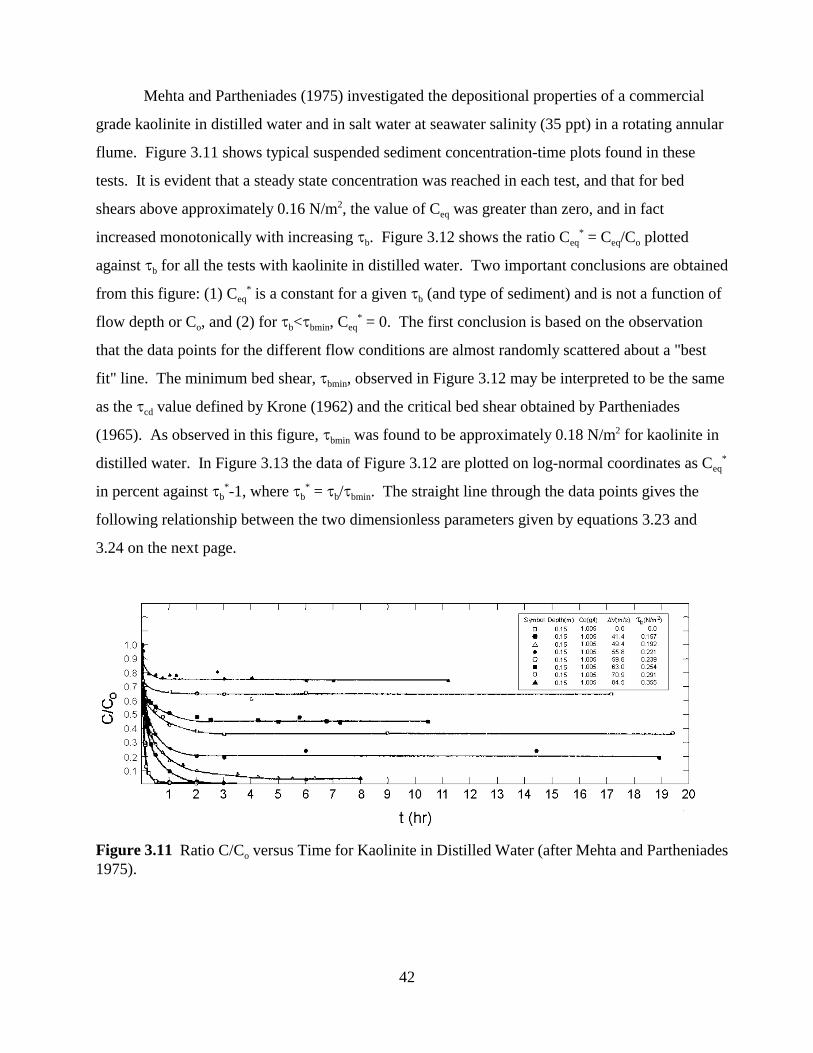
Mehta and Partheniades (1975) investigated the depositional properties of a commercial
grade kaolinite in distilled water and in salt water at seawater salinity (35 ppt) in a rotating annular
flume. Figure 3.11 shows typical suspended sediment concentration-time plots found in these
tests. It is evident that a steady state concentration was reached in each test, and that for bed
shears above approximately 0.16 N/m2, the value of Ceq was greater than zero, and in fact
increased monotonically with increasing Jb. Figure 3.12 shows the ratio Ceq* = Ceq/Co plotted
against Jb for all the tests with kaolinite in distilled water. Two important conclusions are obtained
from this figure: (1) Ceq* is a constant for a given Jb (and type of sediment) and is not a function of
flow depth or Co, and (2) for Jb<Jbmin, Ceq* = 0. The first conclusion is based on the observation
that the data points for the different flow conditions are almost randomly scattered about a "best
fit" line. The minimum bed shear, Jbmin, observed in Figure 3.12 may be interpreted to be the same
as the Jcd value defined by Krone (1962) and the critical bed shear obtained by Partheniades
(1965). As observed in this figure, Jbmin was found to be approximately 0.18 N/m2 for kaolinite in
distilled water. In Figure 3.13 the data of Figure 3.12 are plotted on log-normal coordinates as Ceq*
*in percent against Jb -1, where Jb* = Jb/Jbmin. The straight line through the data points gives the
following relationship between the two dimensionless parameters given by equations 3.23 and
3.24 on the next page.
Figure 3.11 Ratio C/Co versus Time for Kaolinite in Distilled Water (after Mehta and Partheniades 1975).
42
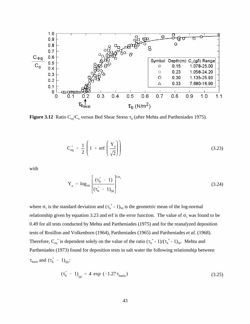
Figure 3.12 Ratio Ceq/Co versus Bed Shear Stress Jb (after Mehta and Partheniades 1975).
Y C ( 1 a
' 1 % erf (3.23)eq 2 2
with
(J( & 1) 1/F1
bY ' log10 (3.24)a (J(
b & 1)50
where F1 is the standard deviation and (Jb* - 1)50 is the geometric mean of the log-normal
relationship given by equation 3.23 and erf is the error function. The value of F1 was found to be
0.49 for all tests conducted by Mehta and Partheniades (1975) and for the reanalyzed deposition
tests of Rosillon and Volkenborn (1964), Partheniades (1965) and Partheniades et al. (1968). *Therefore, Ceq
* is dependent solely on the value of the ratio (Jb - 1)/(Jb* - 1)50. Mehta and
Partheniades (1973) found for deposition tests in salt water the following relationship between
Jbmin and (J( & 1)50 :b
(J( & 1) ' 4 exp (&1.27 Jbmin ) (3.25)b 50
43
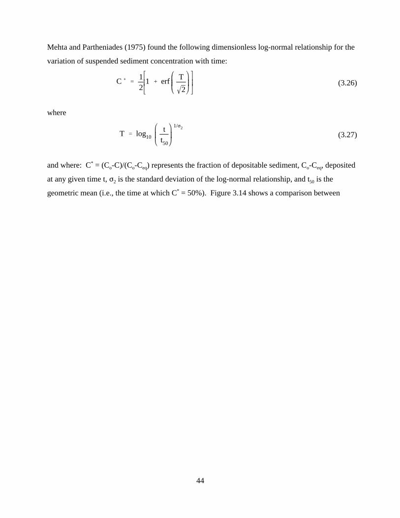
Mehta and Partheniades (1975) found the following dimensionless log-normal relationship for the
variation of suspended sediment concentration with time:
C ( 1 T' 1 % erf (3.26)
2 2
where
1/F2tT ' log10 (3.27)t50
and where: C* = (Co-C)/(Co-Ceq) represents the fraction of depositable sediment, Co-Ceq, deposited
at any given time t, F2 is the standard deviation of the log-normal relationship, and t50 is the
geometric mean (i.e., the time at which C* = 50%). Figure 3.14 shows a comparison between
44
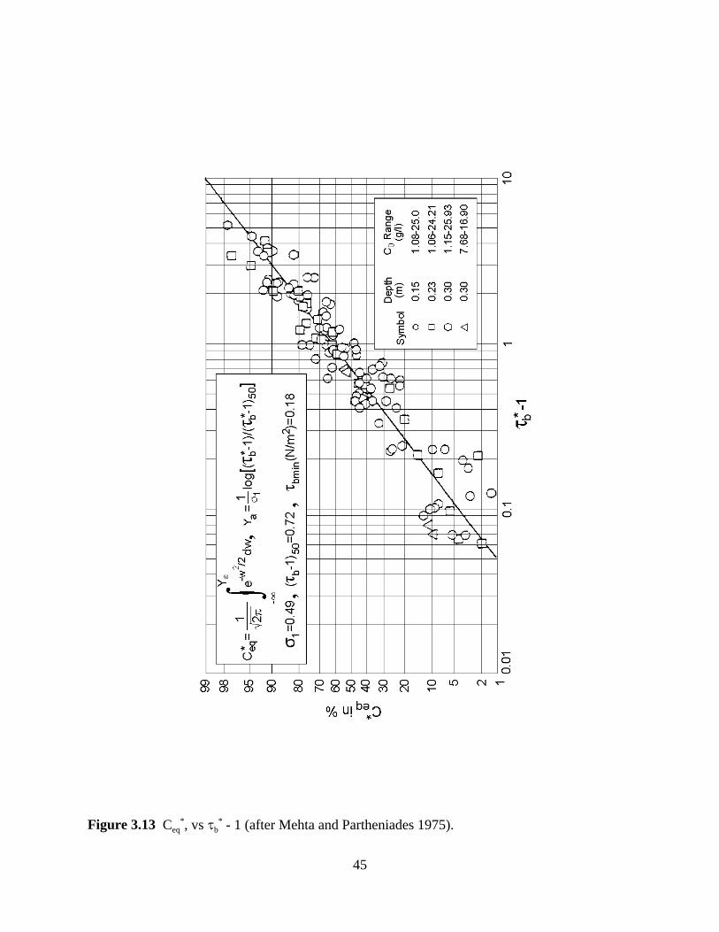
*Figure 3.13 Ceq , vs Jb* - 1 (after Mehta and Partheniades 1975).
45
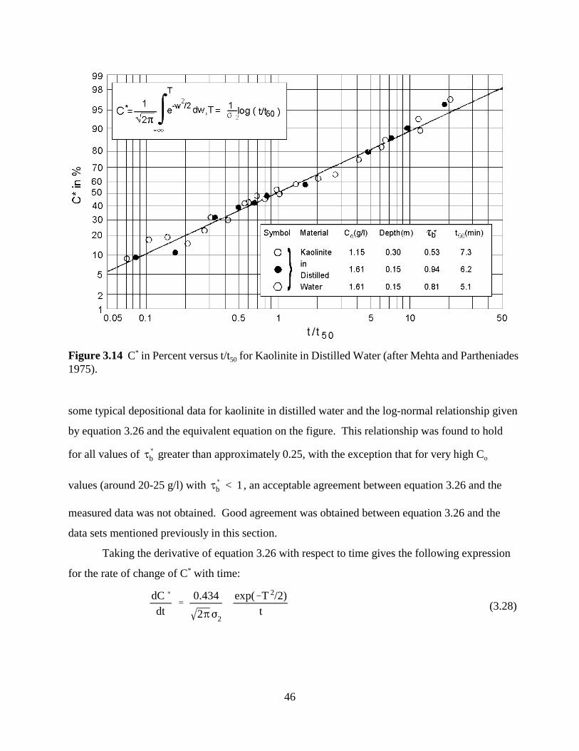
Figure 3.14 C* in Percent versus t/t50 for Kaolinite in Distilled Water (after Mehta and Partheniades 1975).
some typical depositional data for kaolinite in distilled water and the log-normal relationship given
by equation 3.26 and the equivalent equation on the figure. This relationship was found to hold
for all values of J( greater than approximately 0.25, with the exception that for very high Cob
values (around 20-25 g/l) with J( < 1, an acceptable agreement between equation 3.26 and the b
measured data was not obtained. Good agreement was obtained between equation 3.26 and the
data sets mentioned previously in this section.
Taking the derivative of equation 3.26 with respect to time gives the following expression
for the rate of change of C* with time:
dC ('
0.434 exp(&T 2/2) (3.28)dt 2BF2
t
46
The standard deviation, F2, and the geometric mean, t50, were found to be functions of J( b
and C . Shown in Figure 3.15 are examples of the relationships found between these parameters. o
Two conclusions were drawn by Mehta (1973). First, for a specific value of J , the deposition( b
rate was minimum. The rate of deposition increased for J( b values both less than and greater than
this specific value, but not as significantly for higher values as for the lower values. However, for
Jb > Jbmax no deposition of suspended sediment occurred. For San Francisco Bay mud in sea water,
Jbmax was determined to be 1.69 N/m2 . Second, for J < 1, the rate of deposition increased with( b
an increase in depth, while for J( b > 1 , the effect of depth on the deposition rate was minimal. As
previously described, the settling velocity of suspended cohesive sediment particles has been
found to be a function of, among other parameters, the suspension concentration (Krone 1962).
Three types of settling are: (1) no mutual interference, (2) mutual interference, and (3) hindered
settling. For very low suspension concentrations, on the order of 0.1-0.7 g/l, the aggregates or
elementary particles settle independently without much mutual interference, and therefore the
settling velocity is independent of C. For concentrations higher than 5 to 10 g/l, the settling
velocity decreases with increasing concentration (Figure 3.17); this is referred to as hindered
settling. At such high concentrations, the sediment suspension, referred to as fluid mud (Bellessort
47
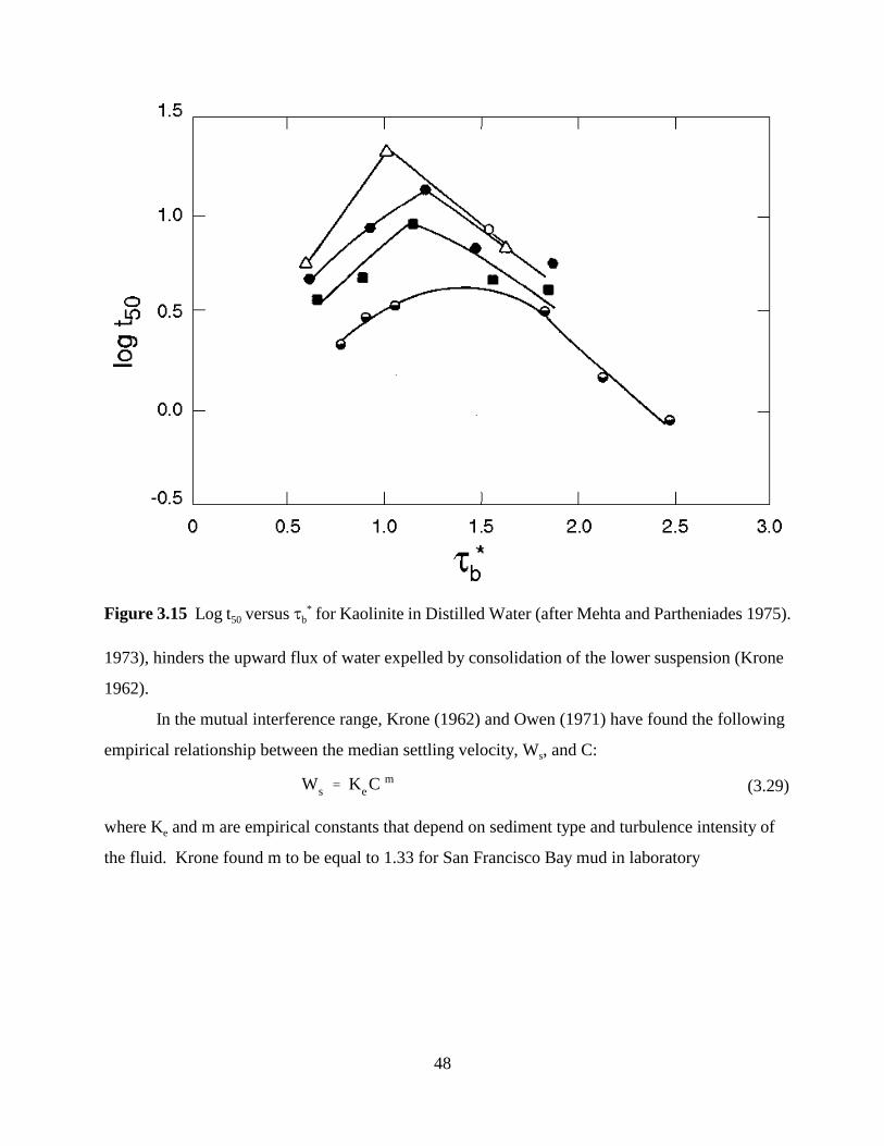
Figure 3.15 Log t50 versus Jb* for Kaolinite in Distilled Water (after Mehta and Partheniades 1975).
1973), hinders the upward flux of water expelled by consolidation of the lower suspension (Krone
1962).
In the mutual interference range, Krone (1962) and Owen (1971) have found the following
empirical relationship between the median settling velocity, Ws, and C:
W ' K C m (3.29)s e
where Ke and m are empirical constants that depend on sediment type and turbulence intensity of
the fluid. Krone found m to be equal to 1.33 for San Francisco Bay mud in laboratory
48
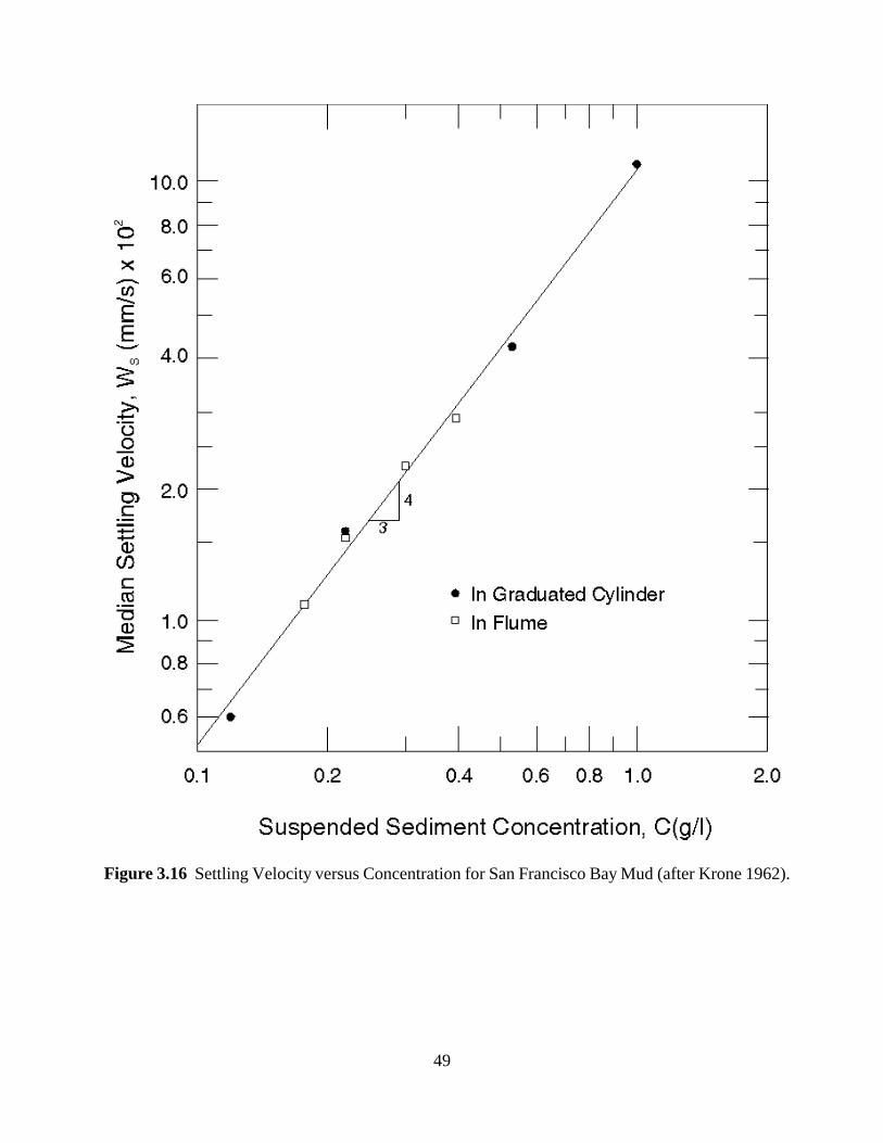
Figure 3.16 Settling Velocity versus Concentration for San Francisco Bay Mud (after Krone 1962).
49
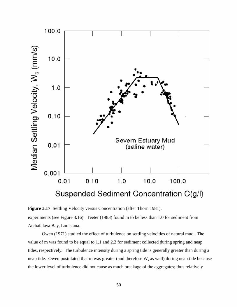
Figure 3.17 Settling Velocity versus Concentration (after Thorn 1981).
experiments (see Figure 3.16). Teeter (1983) found m to be less than 1.0 for sediment from
Atchafalaya Bay, Louisiana.
Owen (1971) studied the effect of turbulence on settling velocities of natural mud. The
value of m was found to be equal to 1.1 and 2.2 for sediment collected during spring and neap
tides, respectively. The turbulence intensity during a spring tide is generally greater than during a
neap tide. Owen postulated that m was greater (and therefore Ws as well) during neap tide because
the lower level of turbulence did not cause as much breakage of the aggregates; thus relatively
50

large aggregates with higher settling velocities were formed. During spring tide, the higher
internal shearing rates resulted in breakage of a higher portion of the aggregates. Thus, small
aggregates with lower settling rates, and therefore lower values of m, were formed.
Migniot (1968) defined a flocculation (coagulation) factor, F, to quantify the effect of
aggregation intensity on Ws:
WsAF ' WsP
(3.30)
where WsA is the median settling velocity of the aggregates and WsP is the median settling velocity
of the elementary sediment particles. Bellessort (1973) found that F varied with grain size
according to F . 250D-1.8 . Wsp-0.9 where D is the mean diameter of the particles in micrometers
and Ws is measured in mm/s. Figure 3.18 shows the effect of particle size on F and WsA for
numerous sediment samples at Co = 10 g/l and salinity S = 30 ppt. Also plotted in this figure is the
variation of F with D found by Dixit et al. (1982) using mud from Atchafalaya Bay, Louisiana. In
these data, however, Co varied from 1.2 to 11 g/l and S - 0.0 ppt. Another important difference
between the two data sets is that Bellessort measured WsA under quiescent conditions, whereas
Dixit et al. (1982) measured the settling velocity under turbulent flow in a rotating annular flume.
As observed, these data have the same slope between F and D as found by Bellessort. This
suggests that, in general, F may be proportional to D-1.8, albeit with different intercept values, at
least for suspension concentrations with Co = 1.2-11 g/l and 0 < S < 30 ppt.
3.2.2.9.1 Effect of Salinity on Deposition - The larger, stronger aggregates of natural
muds formed in a saline medium have been found to result in higher settling velocities (Krone
1962; Owen 1970a). Thus, the effect of salinity on deposition of cohesive sediments may be
quantified in terms of a relationship between salinity and median settling velocity, Ws.
Krone (1962) studied the effect of salinity and suspended sediment concentration on Ws of
San Francisco Bay sediment. The results from settling tests performed under quiescent conditions
in 1-liter cylinders showed the effect of both salinity and suspension concentration on Ws (Figure
3.19). The influence of salinity on Ws is especially significant in the range of 0
51
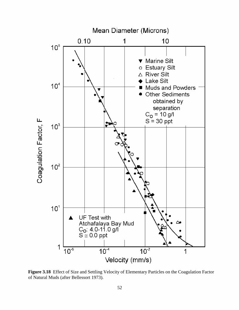
Figure 3.18 Effect of Size and Settling Velocity of Elementary Particles on the Coagulation Factor of Natural Muds (after Bellessort 1973).
52
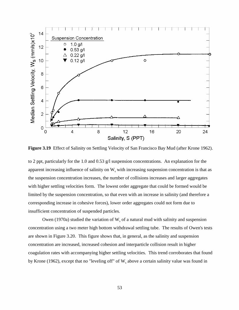
Figure 3.19 Effect of Salinity on Settling Velocity of San Francisco Bay Mud (after Krone 1962).
to 2 ppt, particularly for the 1.0 and 0.53 g/l suspension concentrations. An explanation for the
apparent increasing influence of salinity on Ws with increasing suspension concentration is that as
the suspension concentration increases, the number of collisions increases and larger aggregates
with higher settling velocities form. The lowest order aggregate that could be formed would be
limited by the suspension concentration, so that even with an increase in salinity (and therefore a
corresponding increase in cohesive forces), lower order aggregates could not form due to
insufficient concentration of suspended particles.
Owen (1970a) studied the variation of Ws of a natural mud with salinity and suspension
concentration using a two meter high bottom withdrawal settling tube. The results of Owen's tests
are shown in Figure 3.20. This figure shows that, in general, as the salinity and suspension
concentration are increased, increased cohesion and interparticle collision result in higher
coagulation rates with accompanying higher settling velocities. This trend corroborates that found
by Krone (1962), except that no "leveling off" of Ws above a certain salinity value was found in
53
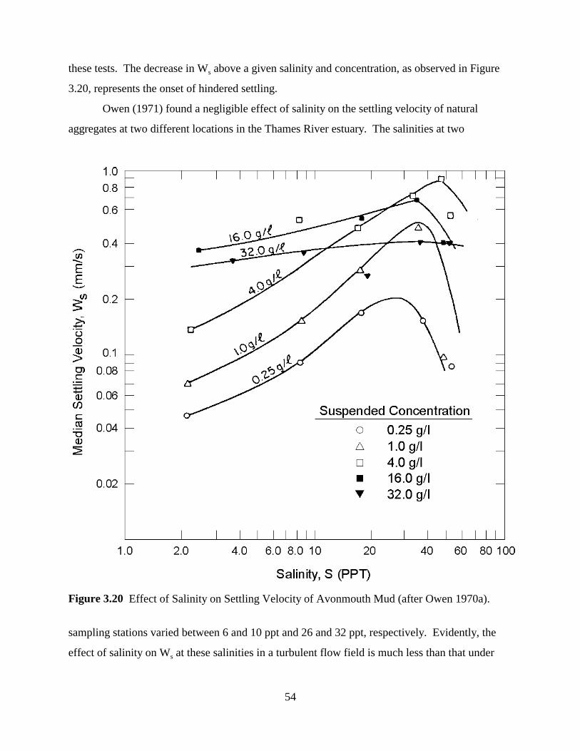
these tests. The decrease in Ws above a given salinity and concentration, as observed in Figure
3.20, represents the onset of hindered settling.
Owen (1971) found a negligible effect of salinity on the settling velocity of natural
aggregates at two different locations in the Thames River estuary. The salinities at two
Figure 3.20 Effect of Salinity on Settling Velocity of Avonmouth Mud (after Owen 1970a).
sampling stations varied between 6 and 10 ppt and 26 and 32 ppt, respectively. Evidently, the
effect of salinity on Ws at these salinities in a turbulent flow field is much less than that under
54
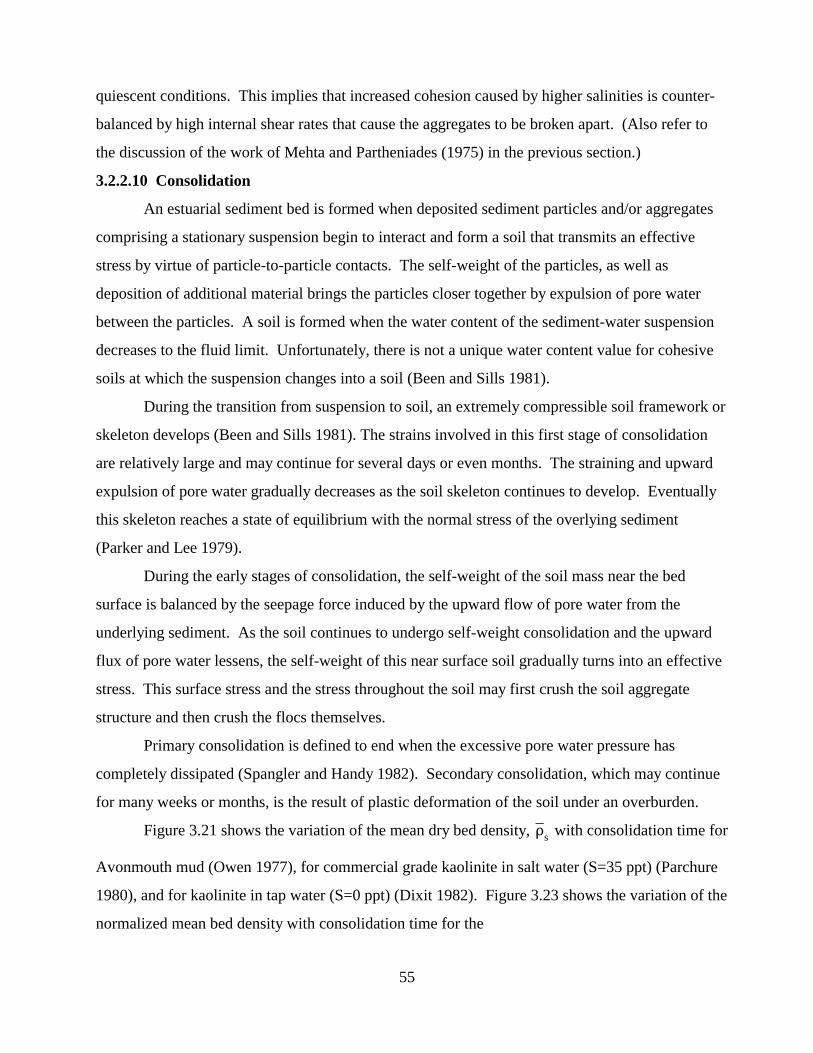
quiescent conditions. This implies that increased cohesion caused by higher salinities is counter
balanced by high internal shear rates that cause the aggregates to be broken apart. (Also refer to
the discussion of the work of Mehta and Partheniades (1975) in the previous section.)
3.2.2.10 Consolidation
An estuarial sediment bed is formed when deposited sediment particles and/or aggregates
comprising a stationary suspension begin to interact and form a soil that transmits an effective
stress by virtue of particle-to-particle contacts. The self-weight of the particles, as well as
deposition of additional material brings the particles closer together by expulsion of pore water
between the particles. A soil is formed when the water content of the sediment-water suspension
decreases to the fluid limit. Unfortunately, there is not a unique water content value for cohesive
soils at which the suspension changes into a soil (Been and Sills 1981).
During the transition from suspension to soil, an extremely compressible soil framework or
skeleton develops (Been and Sills 1981). The strains involved in this first stage of consolidation
are relatively large and may continue for several days or even months. The straining and upward
expulsion of pore water gradually decreases as the soil skeleton continues to develop. Eventually
this skeleton reaches a state of equilibrium with the normal stress of the overlying sediment
(Parker and Lee 1979).
During the early stages of consolidation, the self-weight of the soil mass near the bed
surface is balanced by the seepage force induced by the upward flow of pore water from the
underlying sediment. As the soil continues to undergo self-weight consolidation and the upward
flux of pore water lessens, the self-weight of this near surface soil gradually turns into an effective
stress. This surface stress and the stress throughout the soil may first crush the soil aggregate
structure and then crush the flocs themselves.
Primary consolidation is defined to end when the excessive pore water pressure has
completely dissipated (Spangler and Handy 1982). Secondary consolidation, which may continue
for many weeks or months, is the result of plastic deformation of the soil under an overburden.
Figure 3.21 shows the variation of the mean dry bed density, D s with consolidation time for¯
Avonmouth mud (Owen 1977), for commercial grade kaolinite in salt water (S=35 ppt) (Parchure
1980), and for kaolinite in tap water (S=0 ppt) (Dixit 1982). Figure 3.23 shows the variation of the
normalized mean bed density with consolidation time for the
55
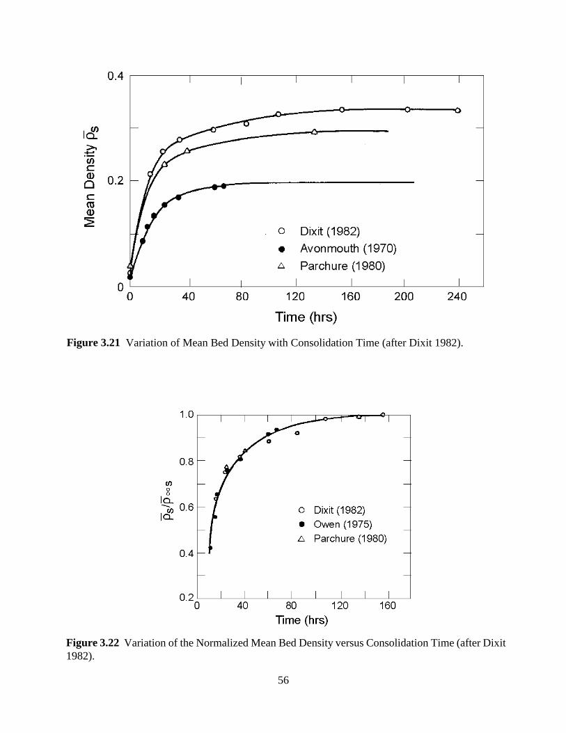
Figure 3.21 Variation of Mean Bed Density with Consolidation Time (after Dixit 1982).
Figure 3.22 Variation of the Normalized Mean Bed Density versus Consolidation Time (after Dixit 1982).
56
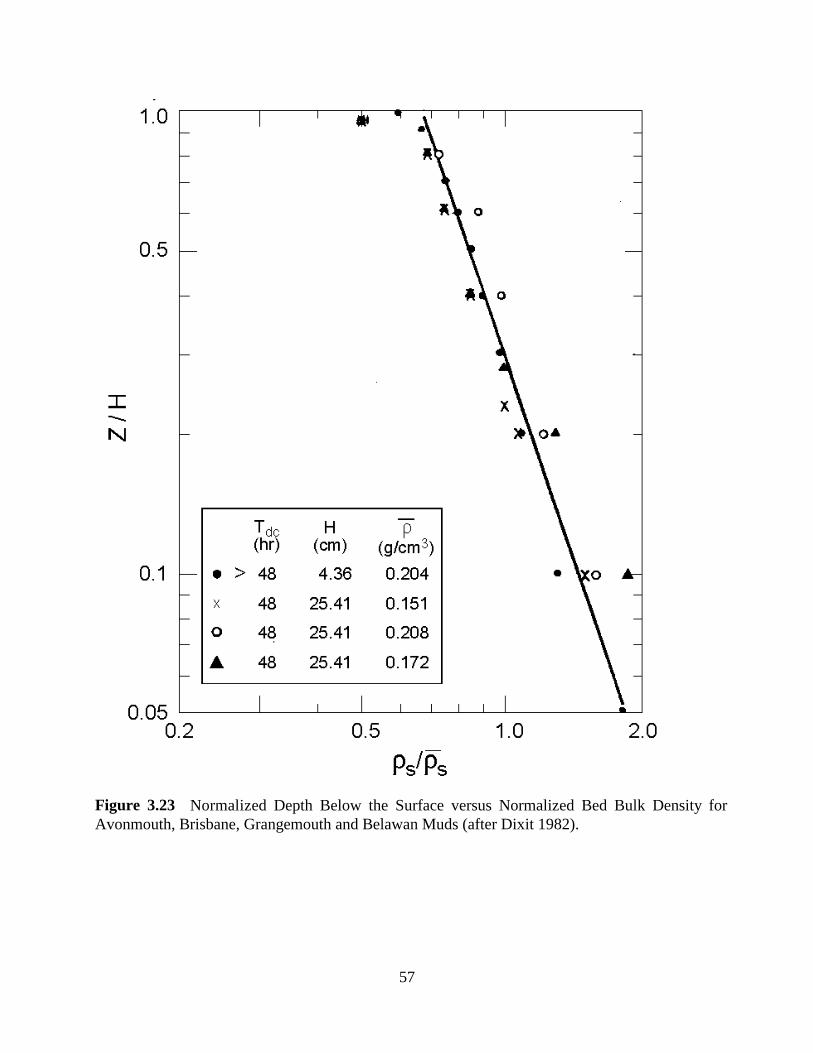
Figure 3.23 Normalized Depth Below the Surface versus Normalized Bed Bulk Density for Avonmouth, Brisbane, Grangemouth and Belawan Muds (after Dixit 1982).
57
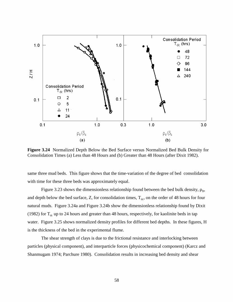
Figure 3.24 Normalized Depth Below the Bed Surface versus Normalized Bed Bulk Density for Consolidation Times (a) Less than 48 Hours and (b) Greater than 48 Hours (after Dixit 1982).
same three mud beds. This figure shows that the time-variation of the degree of bed consolidation
with time for these three beds was approximately equal.
Figure 3.23 shows the dimensionless relationship found between the bed bulk density, DB,
and depth below the bed surface, Z, for consolidation times, Tdc, on the order of 48 hours for four
natural muds. Figure 3.24a and Figure 3.24b show the dimensionless relationship found by Dixit
(1982) for Tdc up to 24 hours and greater than 48 hours, respectively, for kaolinite beds in tap
water. Figure 3.25 shows normalized density profiles for different bed depths. In these figures, H
is the thickness of the bed in the experimental flume.
The shear strength of clays is due to the frictional resistance and interlocking between
particles (physical component), and interparticle forces (physicochemical component) (Karcz and
Shanmugam 1974; Parchure 1980). Consolidation results in increasing bed density and shear
58
strength (Hanzawa and Kishida 1981). Figure 3.26 shows the increase in the shear strength profile
with consolidation time for flow-deposited kaolinite beds in tap water.
As mentioned previously, the nature and effect of consolidation on shear strength profiles
of cohesive sediment beds are not well known at present, and the limited information that has been
obtained is often contradictory (Parchure 1980). Figure 3.27 shows the correlation found by Owen
(1970b) between the dry sediment density and shear strength for statically deposited beds of
Avonmouth mud. Least squares analysis of the data plotted in this figure gave a slope of 2.44 and
a coefficient of determination of r2 = 0.83. The power expression relating J and D is of the form:c s
J ' 6.85 x 10&6 D2.44 (3.31)c s
Owen considered that the correlation obtained between J and Ds was satisfactory, considering the c
experimental error involved in the measurement of both these parameters.
3.3 COHESIONLESS SEDIMENT TRANSPORT
Cohesionless sediment transport occurs when the hydrodynamic forces (i.e., bed shear)
acting on sediment particles at the bed surface exceed the resisting forces of interparticle friction
and gravity. Thus, estimation of sediment transport requires calculation of the flow induced bed
shear stress (or shear velocity). The equation used in this module to calculate the bed shear stress
is the following Darcy-Weisbach type relationship:
1J ' Df *V*V (3.32)c 2 c
where V = current speed, and fc = current friction factor, given by the well known relationship
from turbulence theories (Christoffersen 1982):
1/22 11.04h
' 2.5 ln (3.33)f kNc
in which kN is Nikuradse's roughness.
Two methods for predicting the non-cohesive sediment transport rate are incorporated in
this module. These are the Einstein methodology (Simons and Senturk 1976) and the
Ackers-White algorithm (Ackers and White 1973). The latter is used only when the median
59
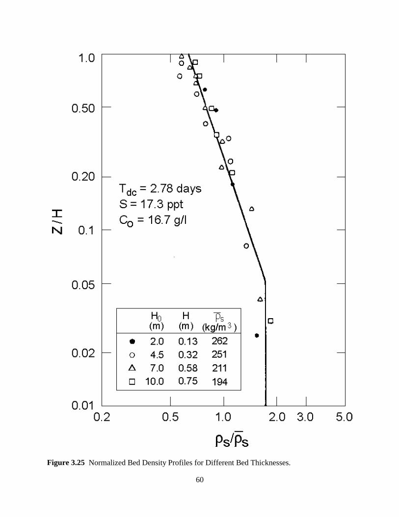
Figure 3.25 Normalized Bed Density Profiles for Different Bed Thicknesses.
60
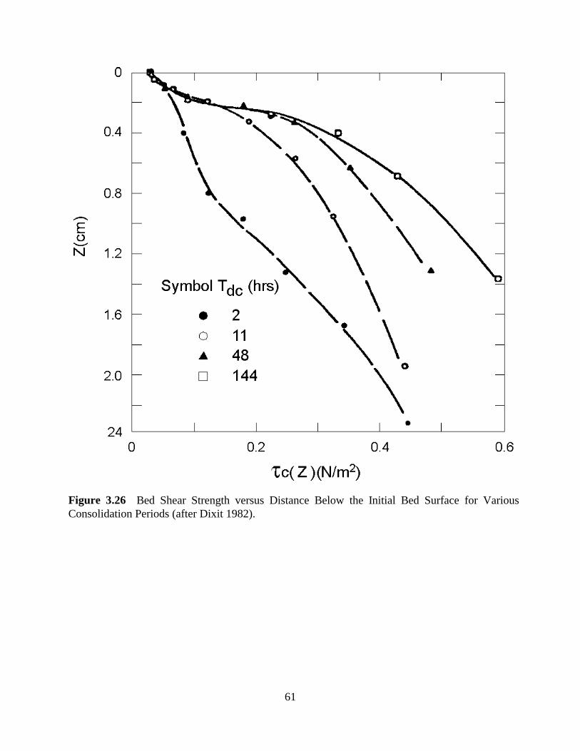
Figure 3.26 Bed Shear Strength versus Distance Below the Initial Bed Surface for Various Consolidation Periods (after Dixit 1982).
61
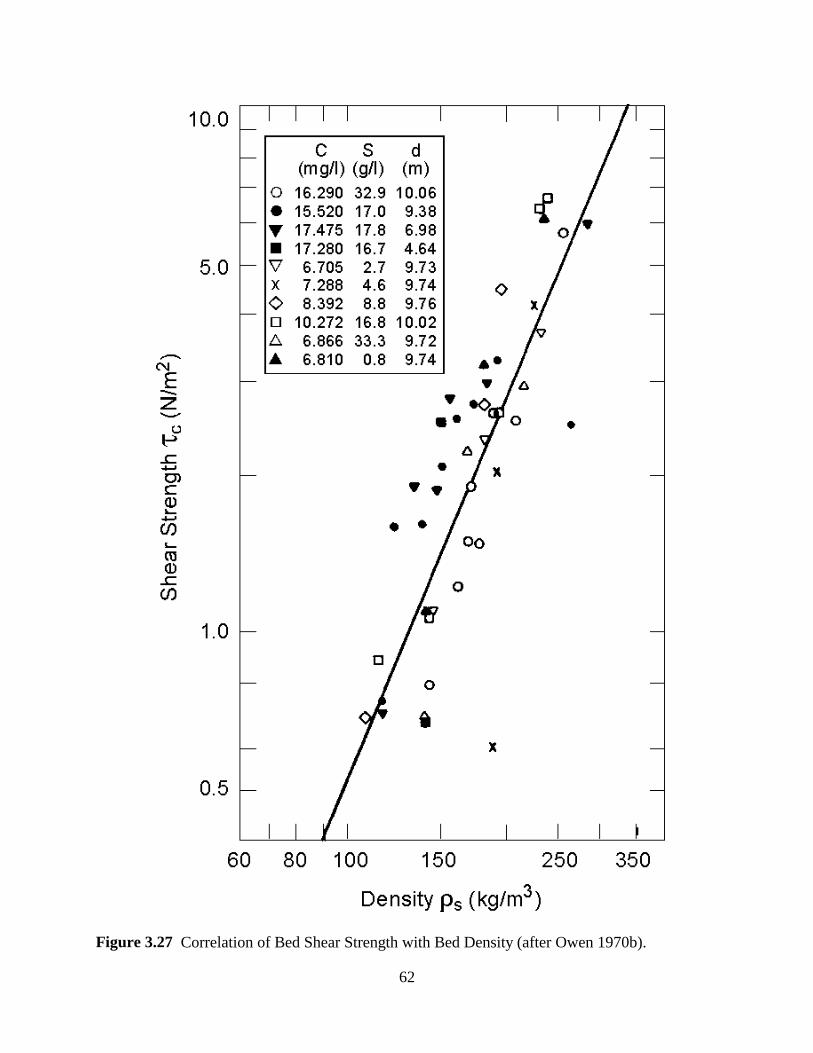
Figure 3.27 Correlation of Bed Shear Strength with Bed Density (after Owen 1970b).
62
diameter, d50, is greater than 0.04 mm. When d50 is greater than 0.04 mm, the normal procedure is
to alternatively use both methods and compare the results.
When sediment transport away from a point is not equal to that towards the same point,
erosion or deposition will occur causing changes in the bottom elevation. Erosion will result if
there is a net transport of sediment away from the point, while deposition will occur if there is a
net sediment transport towards it. Using a control volume approach in two horizontal dimensions,
Fahien (1983) presented a differential balance of sediment volume flux and accretion/scour. The
sediment volume conservation equation is given by
Mb %
Mqx %
Mqy ' 0 (3.34)
Mt Mx My
where b = local bed surface elevation, and qx, qy = components of the sediment load (dry weight)
transport per unit width in the x- and y-directions, respectively, as determined using either the
Einstein or Ackers-White equation. Equation 3.34 is used in the sediment transport module to
estimate the local (i.e., at each node) bottom elevation change resulting from net sediment
transport to or away from a given location. The elevation change at each node during a single time
step is computed after the hydrodynamic and sediment transport computations are completed. The
predicted bathymetric changes at a given time step are used in the hydrodynamic module during
the next time step to predict the new flow field.
3.4 CONTAMINANT TRANSPORT
The transport of both cohesionless sediments (i.e., medium size silts and larger particles)
and fine grain cohesive sediments (i.e., mostly composed of terrigenous clay size particles and fine
silts; sometimes includes small quantities of biogenic detritus, algae, and organic matter) must be
modeled to account for adsorption and desorption of contaminants onto and from sediments of all
sizes. The properties of clays which cause the sorption of contaminants are their large specific
area, surficial negative electrical charge, and their cation exchange capacity. Particulate
contaminants may be sorbed on the mineral, oxide or hydrous oxide surfaces; bonded in humic
materials; precipitated as metal sulfides; sorbed on the exchange sites of clay minerals; or
incorporated in the detrital organic or mineral phase associated with all sizes of sediment particles.
63
The bulk of the contaminant load in surface waters is in fact quite often transported sorbed
to cohesive sediments rather than in the desorbed state (Kirby and Parker 1973). In addition, the
portion of the contaminant load adsorbed to cohesionless sediments is often less than that sorbed
to cohesive sediments. This follows from studies that have shown that increasing metal
concentrations typically correlate positively with decreasing sediment particle size, increasing
sediment specific area, and increasing concentrations of organic matter and manganese and iron
oxides (Horowitz and Elrick 1987). However, there are exceptions to this trend. Studies by
Moore et al. (undated) and Brook and Moore (undated), found weak correlation between percent
of fine grained sediment (less that 63 microns) and trace metal concentrations in the Clark Fork
River in Montana, while coarse grain sediments contributed significantly to bulk metal
concentrations. This emphasizes the need to consider the transport of both cohesive and
cohesionless sediments in contaminant transport modeling.
Processes that affect the association of inorganic contaminants with aquatic sediments
include adsorption/desorption, complexation, and organic coatings (Dzombak and Morel 1987).
These processes have been the subject of several studies, and are covered in detail elsewhere (e.g.,
Stumm and Morgan 1981). The processes of sorption and desorption are discussed below.
Biological factors (e.g., presence of organic coatings on sorbents), which often have a significant
effect on adsorption processes, are not discussed.
Sorption of contaminants generally refers to both adsorption and absorption (Elzerman and
Coates 1987). Adsorption of a sorbate to a sorbent occurs at a surface or interface, while
absorption continues beyond the interface and involves incorporation of the sorbate into the
interior of the sorbent. Distinction between these two processes is usually not precise, thus
explaining the use of the collective term sorption. Sorption of inorganic compounds is described
as a chemical coordination process involving certain reactions between absorbents and the
inorganic adsorbate (Dzombak and Morel 1987). Adsorption models for inorganic contaminants
should simulate these chemical reactions and account for interaction between electrical surface
charges and ion adsorption. Such adsorption models are highly empirical in nature due to the
complex electrochemical interactions, and are generally applicable for a specific sorbent-sorbate
pair only (Dzombak and Morel 1987). Desorption is the reverse of sorption. Typically, a
geochemical-metals speciation model (such as MINTEQA2; Brown and Allison 1987), is used to
64
compute metals precipitation and sorption/desorption for the geochemical conditions at the site of
interest.
A partition coefficient, Kp, is used to define the distribution of a contaminant between the
particulate and dissolved phase concentration. Reported values of Kp usually correspond to
equilibrium conditions, at which rates of desorption and sorption are equal. Despite typically high
partition coefficients, the total mass of contaminants sorbed to suspended sediments is usually
lower than that in the dissolved phase because of relatively low concentrations of suspended
sediment. In addition, the sorbed contaminant mass on bed sediments, which can be large, has to
be considered. Contaminants that are sorbed on bed sediments either sorbed directly onto the
deposited sediments or sorbed onto suspended sediments which subsequently settled to the bed. In
general, there are few limitations to benthic exchange, with the bed acting like a capacitor that
tends to maintain elevated concentrations in the water column (Medine and McCutcheon 1989).
The partition coefficient is given by:
C f p ' pKp '
CdC fdC (3.35)
s s
with Cp = particulate contaminant concentration [kg/m3] (adsorbed contaminant mass/total
volume of water);
Cd = dissolved contaminant concentration [kg/m3] (dissolved contaminant mass/total
volume of water);
Cs = mass concentration of suspended sediment [kg/m3] (mass of sediments/total volume of
water);
fp = fraction of contaminant in the particulate phase = Cp/Ct;
fd = fraction of contaminant in the dissolved phase = Cd/Ct; and
Ct = total contaminant concentration [kg/m3] = Cp + Cd.
Values for partition coefficients can be determined through laboratory testing using the most
prevalent or critical dissolved contaminant and environmental parameters (e.g., pH, temperature,
conductivity) representative of field conditions. However, field studies are preferred to yield
values that more realistically represent the actual field environment.
65
Sorption of contaminants onto both suspended and deposited sediments is usually treated
as a process in thermodynamic equilibrium that occurs rapidly compared to transformation
processes such as hydrolysis, microbial transformation, photolysis, volatilization, and chemical
oxidation. These slower processes should be simulated using a kinetic approach (Baughman and
Burns 1980). The rates at which sorption and desorption take place have been found to vary
inversely with the partition coefficient, and therefore are slower for chemicals which more strongly
sorb onto particular sorbents, e.g., cohesive sediments. It is often assumed that sorption/desorption
occurs instantaneously, or within one time step in a contaminant transport model. The validity of
this assumption is dependent on sorption rates between the contaminant and sediment.
Factors which collectively control the distribution and fate of a contaminant in an aquatic
environment have been classified according to system, sorbent (sediment), and sorbate
(contaminant) characteristics (Elzerman and Coates 1987). System characteristics include, among
others, the following : a) transport of water; transport and fate of sediment; nature or contaminant
loading to the system; and b) temperature; pH; ionic strength; concentration gradient of
contaminant; and competing sorbates and sorbents. The items listed under a) are macro-system
factors, while those given under b) are defined as micro-system factors that are important close to
the sorbent surface. The item listed as 'nature of contaminant loading' refers to quantity, location,
timing, and mode (i.e., point or non-point source) of contaminant release. Sorbent characteristics
include the following: composition; size; shape; pore structure; and surface electrochemical
charges. Sorbate characteristics include molecular structure, which itself is controlled by polarity,
size, shape and electric charge. The effects of each of these components on contaminant transport
and transformations in aquatic systems are discussed in detail by Karickhoff (1981), Lyman
(1985), Elzerman and Coates (1987), and Dzombak and Morel (1987).
In HSCTM-2D, adsorption of dissolved contaminants onto suspended sediments and onto
the bed surface and desorption of particulate contaminants from these surfaces into the water
column are the modeled physico-chemical processes that affect the distribution and fate of
contaminants. Other processes that typically affect the fate and transport of contaminants in
surface water environments such as volatilization, bioconcentration, biouptake, and bioturbation
are not incorporated in HSCTM-2D. The adsorption module used in HSCTM-2D is a so-called
thermodynamic equilibrium model that assumes constant partitioning between the dissolved
66
(solute) phase and particulate (solid) phase. Equilibrium models that use a single "black box"
partition coefficient are typically used to avoid the complexities of the kinetics of the adsorption
and desorption processes. However, consistent relationships between the partition coefficients and
environmental parameters such as temperature, conductivity and pH have not yet been found.
Thus, equilibrium adsorption/desorption models such as the one in HSCTM-2D are based on the
following assumptions:
a. Local equilibrium between solute and solid phases is instantaneously achieved. Thomann
and DiToro (1983) found that equilibrium is usually attained within minutes. Thus,
assuming that equilibrium is achieved over one time-step in the model is very reasonable.
b. The relationship between dissolved and particulate concentrations given by the adsorption
isotherm is approximately linear for low contaminant concentrations (O'Connor 1980).
Hence, a single partition coefficient can be used in an equilibrium adsorption model. This
coefficient can be inferred from either the Freundlich or Langmuir isotherms (Schnoor et
at. 1987).
c. The adsorption and desorption processes are completely reversible. Thus, a single partition
coefficient can be used to represent both processes.
The total contaminant concentration, Ct [kg/m3], is given by:
Ct = Cp + Cd = Cd(1 + KpCs) (3.36)
Partition coefficients can be determined in laboratory experiments using sorbent species most
prevalent in the field and environmental conditions representative of field conditions (Thomann
and DiToro 1983). Ideally, however, field studies should be performed to determine partition
coefficient values that more realistically represent natural conditions (HydroQual, Inc. 1982).
Dissolved Contaminant Transport Module - The following processes are accounted for in
modeling the advective and dispersive transport of a maximum of three dissolved contaminants:
sorption, desorption, chemical degradation or decay, and local (point) sources of contaminants.
Contaminant-sediment interaction, by the processes of sorption and desorption is simulated to
occur between dissolved contaminants and sediments in suspension and deposited on the bed.
The governing equation for dissolved contaminant transport is equation 3.13 with C = Cd
(where Cd = dissolved contaminant mass concentration) and ST given by
67

DiS ' & j Ki(KpiCdCsi & Cpi) & j Ki(i(1&P) KdCd %h
Di (3.37)
j Ki(i(1&P) (Cp)B % Sd & 8Cdh
where Ki = sorption or desorption rate to approach equilibrium with the ith sediment fraction; Kpi =
partition coefficient between particulate contaminant associated with ith sediment and dissolved
contaminant; Csi = suspended mass concentration associated with ith sediment; Cpi = particulate
contaminant concentration associated with ith sediment; P = porosity of the sediment bed; Di =
diameter of the ith sediment in the bed [m]; (i = density of ith sediment in the bed [kg/m3]; (Cp)Bi =
particulate contaminant concentration associated with the ith sediment in the bed; 8 = bio
chemical degradation rate or radionuclide decay rate [s-1]; and Sd = source strength of dissolved
contaminant [kg/m3s]. The two terms inside the first summation on the right hand side of equation
3.37 represent the adsorption rate of dissolved contaminants and the desorption rate of particulate
contaminants onto and from suspended sediments, respectively. The next two terms represent the
rate of absorption of dissolved contaminants onto bed sediments (i.e., sink) and the rate of
desorption of particulate contaminants from bed sediments into the water column (i.e., source),
respectively.
Particulate Contaminant Transport Module - The following processes are accounted for in
modeling the transport of up to three particulate contaminants: adsorption, desorption, local
sources/sinks, and chemical degradation. Sorption occurs when a dissolved contaminant bonds to
a sediment particle, at which time it becomes a particulate contaminant. When the latter desorbs
from the sediment it again becomes a dissolved contaminant. The transport of contaminants
sorbed to sediments is determined separately for each of the three size fractions.
The governing equation for particulate contaminant transport is equation 3.13 with C = Cpi
and ST given by
d eS ' j [&Ki(Cpi&KpiCsiCd)% Cpi% (Cpi)B%Spi&8Cpi] (3.38)
h h
68
where Spi = source strength of particulate contaminant associated with the ith sediment fraction
[kg/m3s]. The first two terms on the right hand side of equation 3.38 represent the desorption rate
of particulate contaminants and the adsorption rate of dissolved contaminants from and onto
suspended sediments, respectively. The third and fourth terms represent the deposition rate and
resuspension rate of particulate contaminants, respectively.
69
SECTION 4
FINITE ELEMENT METHOD
4.1 INTRODUCTORY NOTE
The finite element method (FEM) is used to solve the shallow water flow equations (eqs.
3.1, 3.7 and 3.8) and the advection-dispersion equation (eq. 3.12). The discretization procedures
used in the FEM reduce the equations to be solved to ones with a finite number of dependent
variables by dividing the continuous solution domain into a number of elements and by expressing
the dependent variables in terms of approximating interpolation (i.e., shape) functions within each
element. The values of the dependent variables at node points are used to define the interpolation
functions. Node points are usually located on the boundaries of elements and are used to define
the connection between adjacent elements. The number and location of node points must be
chosen such that continuity of the dependent variables across common boundaries of adjacent
elements is achieved (Zienkiewicz 1977). The behavior of the dependent variables within each
element is defined by the values of the dependent variables at the nodes and the shape function.
Then the errors which results from use of the approximate dependent variables are minimized.
This procedure results in a set of simultaneous equations which are solved for the unknown nodal
dependent variables at the next time step. A detailed description of the method is presented by
Zienkiewicz (1977).
70
4.2 DESCRIPTION
4.2.1 Interpolation Functions
The global and local element coordinate systems are shown in Figure 4.1a and Figure 4.1b,
respectively. The global x,y coordinate system is continuous over the entire solution domain,
whereas the local element >, 0 coordinate system applies only within an element. The local
coordinate systems for a quadratic quadrilateral and a quadratic right triangular element are shown
in Figure 4.1b.
Because three nodes are used along each side of the triangular and quadrilateral elements in
HSCTM-2D, quadratic shape functions are required. The quadratic shape functions in HSCTM
2D determine the values of both the dependent variables and element geometry. Thus, the
elements are isoparametric (Zienkiewicz 1977). There is one shape function, Ni, for every node in
a given element. Thus, for triangular elements there are six shape functions; for quadrilateral
elements, there are eight. The shape functions are functions of the local coordinates > and 0 and
the values of > and 0 at the nodal points. The quadratic shape functions for quadrilateral and
triangular elements are given in Table 4.1. The parameters >i and 0i in this table are the nodal
coordinates.
A dependent variable, e.g., C, is approximated as the following function of the unknown
nodal point concentrations, Ci, and the shape functions, Ni:
ñ i
j'nn
Cj NiCi (4.1) i'1
˜where C = approximate suspended sediment concentration at any location inside the jth element, j
and nn = number of nodes forming the jth element.
71
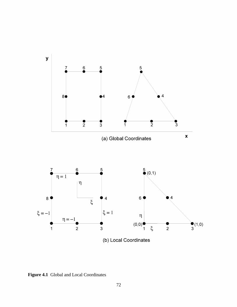
Figure 4.1 Global and Local Coordinates
72
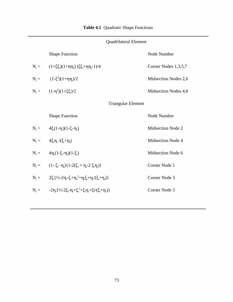
Table 4.1 Quadratic Shape Functions
Shape Function
Ni = (1+>>i)(1+00i) (>>i+00i-1)/4
Ni = (1->2)(1+00i)/2
Ni = (1-02)(1+>>i)/2
Shape Function
Ni = 4>i(1-0i)(1->i-0i)
Ni = 4>i0i /(>i+0i)
Ni = 40i(1->i-0i)(1->i)
Ni = (1- >i- 0i){1-2(>i + 0i-2 >i0i)}
Ni = 2>i{½-20i->i+0i2+0i>i+0i/(>i+0i)}
Ni = -20i{½-2>i-0i+>i2+>i0i+>i/(>i+0i)}
Quadrilateral Element
Triangular Element
Node Number
Corner Nodes 1,3,5,7
Midsection Nodes 2,6
Midsection Nodes 4,8
Node Number
Midsection Node 2
Midsection Node 4
Midsection Node 6
Corner Node 1
Corner Node 3
Corner Node 5
73
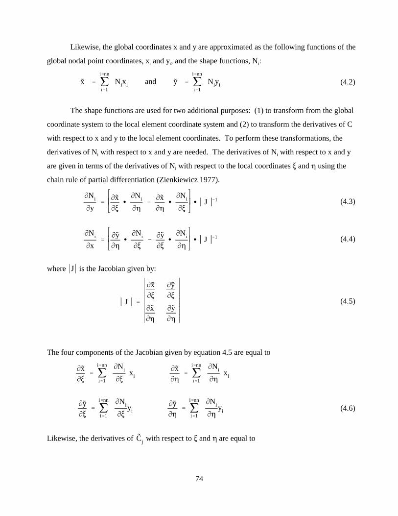
Likewise, the global coordinates x and y are approximated as the following functions of the
global nodal point coordinates, xi and yi, and the shape functions, Ni:
x 'i'nn
j Nixi and y 'i'nn
j Niyi (4.2) i'1 i'1
The shape functions are used for two additional purposes: (1) to transform from the global
coordinate system to the local element coordinate system and (2) to transform the derivatives of C
with respect to x and y to the local element coordinates. To perform these transformations, the
derivatives of Ni with respect to x and y are needed. The derivatives of Ni with respect to x and y
are given in terms of the derivatives of Ni with respect to the local coordinates > and 0 using the
chain rule of partial differentiation (Zienkiewicz 1977).
MNi
My ' M x
M> C
MNi
M0 & M x
M0 C
MNi
M> C J &1 (4.3)
MNi
Mx ' My
M0 C
MNi
M> & My
M> C
MNi
M0 C J &1 (4.4)
where *J* is the Jacobian given by:
/00000000000
M x M>
My M> /00000000000
J ' M x My
(4.5)
M0 M0
The four components of the Jacobian given by equation 4.5 are equal to
i'nn
ji'nn
jMNi MNiMx
M> Mx
' 'xi xiM0 M0M>i'1 i'1
i'nn
ji'nn
jMNi MNiMy My
' ' (4.6)yi yiM0 M0M> M>i'1 i'1
˜Likewise, the derivatives of Cj with respect to > and 0 are equal to
74
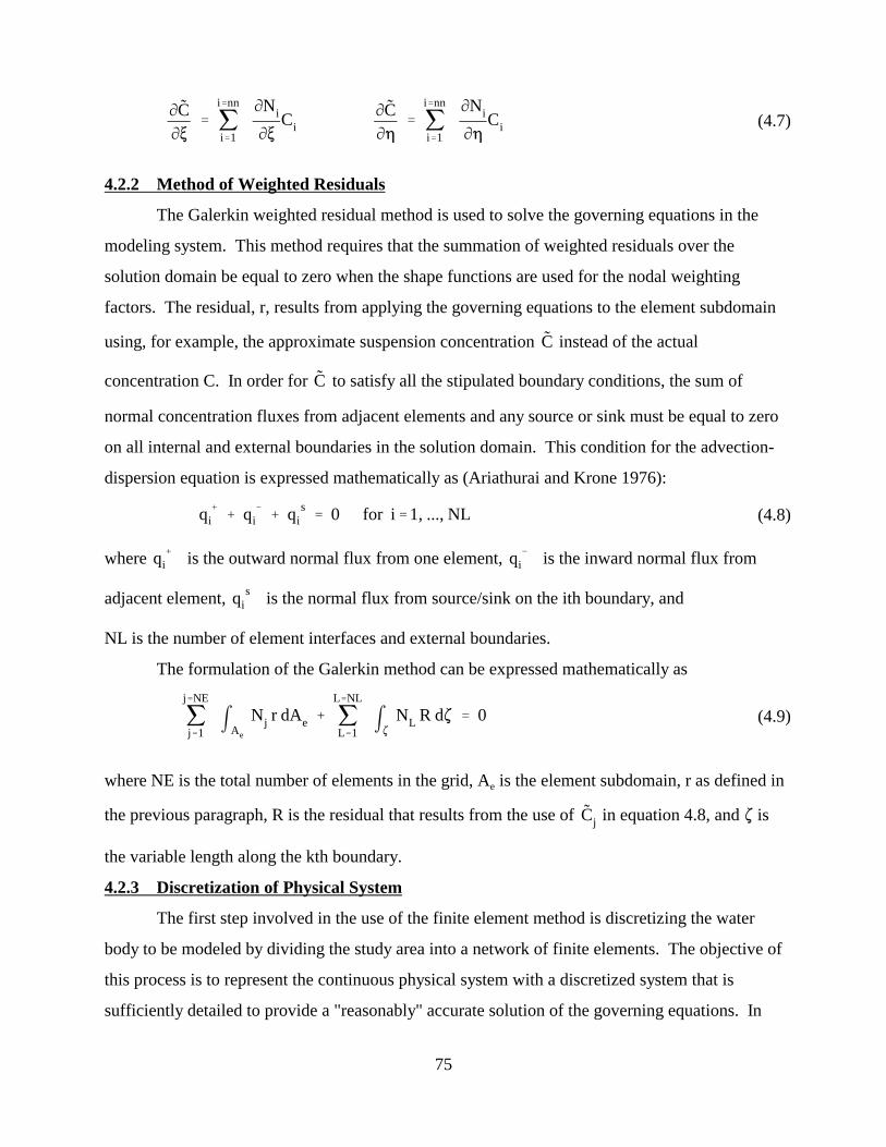
i
j'nn MNi
i
j'nn MNiM M C
' Ci C
' Ci (4.7)M> i'1 M> M0 i'1 M0
4.2.2 Method of Weighted Residuals
The Galerkin weighted residual method is used to solve the governing equations in the
modeling system. This method requires that the summation of weighted residuals over the
solution domain be equal to zero when the shape functions are used for the nodal weighting
factors. The residual, r, results from applying the governing equations to the element subdomain
using, for example, the approximate suspension concentration C instead of the actual
concentration C. In order for C to satisfy all the stipulated boundary conditions, the sum of
normal concentration fluxes from adjacent elements and any source or sink must be equal to zero
on all internal and external boundaries in the solution domain. This condition for the advection-
dispersion equation is expressed mathematically as (Ariathurai and Krone 1976):
% q % q & % q s ' 0 for i ' 1, ..., NL (4.8)i i i
where q % is the outward normal flux from one element, q & is the inward normal flux from i i
adjacent element, q s is the normal flux from source/sink on the ith boundary, and i
NL is the number of element interfaces and external boundaries.
The formulation of the Galerkin method can be expressed mathematically as
j'NE L
j'NL
j mANj r dAe % m.
NL R d. ' 0 (4.9) j'1 e L'1
where NE is the total number of elements in the grid, Ae is the element subdomain, r as defined in
˜the previous paragraph, R is the residual that results from the use of Cj in equation 4.8, and . is
the variable length along the kth boundary.
4.2.3 Discretization of Physical System
The first step involved in the use of the finite element method is discretizing the water
body to be modeled by dividing the study area into a network of finite elements. The objective of
this process is to represent the continuous physical system with a discretized system that is
sufficiently detailed to provide a "reasonably" accurate solution of the governing equations. In
75
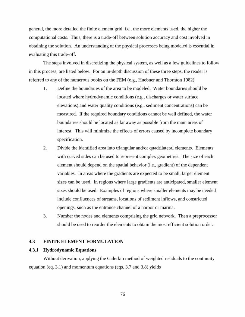
general, the more detailed the finite element grid, i.e., the more elements used, the higher the
computational costs. Thus, there is a trade-off between solution accuracy and cost involved in
obtaining the solution. An understanding of the physical processes being modeled is essential in
evaluating this trade-off.
The steps involved in discretizing the physical system, as well as a few guidelines to follow
in this process, are listed below. For an in-depth discussion of these three steps, the reader is
referred to any of the numerous books on the FEM (e.g., Huebner and Thornton 1982).
1. Define the boundaries of the area to be modeled. Water boundaries should be
located where hydrodynamic conditions (e.g., discharges or water surface
elevations) and water quality conditions (e.g., sediment concentrations) can be
measured. If the required boundary conditions cannot be well defined, the water
boundaries should be located as far away as possible from the main areas of
interest. This will minimize the effects of errors caused by incomplete boundary
specification.
2. Divide the identified area into triangular and/or quadrilateral elements. Elements
with curved sides can be used to represent complex geometries. The size of each
element should depend on the spatial behavior (i.e., gradient) of the dependent
variables. In areas where the gradients are expected to be small, larger element
sizes can be used. In regions where large gradients are anticipated, smaller element
sizes should be used. Examples of regions where smaller elements may be needed
include confluences of streams, locations of sediment inflows, and constricted
openings, such as the entrance channel of a harbor or marina.
3. Number the nodes and elements comprising the grid network. Then a preprocessor
should be used to reorder the elements to obtain the most efficient solution order.
4.3 FINITE ELEMENT FORMULATION
4.3.1 Hydrodynamic Equations
Without derivation, applying the Galerkin method of weighted residuals to the continuity
equation (eq. 3.1) and momentum equations (eqs. 3.7 and 3.8) yields
76
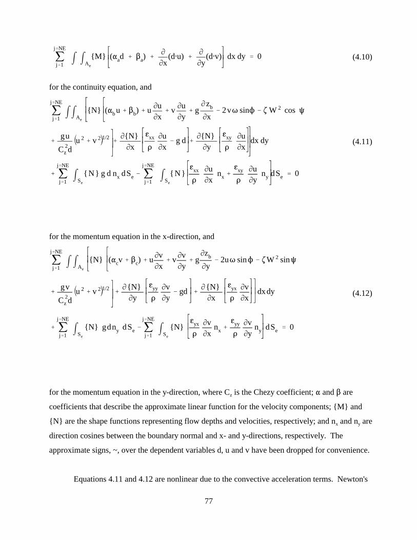
j'NE Mj m mA{M} (" d % $ a) % M (d@u) % (d@v) dx dy ' 0 (4.10)a Mx Myj'1 e
for the continuity equation, and
j'NE Mu M zb{N} (" b u % $b) % u Mu % v % g & 2v T sinN & . W 2 cos Rj mmA Mx My Mxj'1 e
% gu 2 1/2 % M{N} M{N} gxy Mu u 2 % v
gxx Mu & g d % dx dy (4.11)
Mx D Mx My D MxC 2dz
j'NE j'NE gxx Mu gxy Mu% j mS
{ N } g d nx dS & j mS{N} n % n dS ' 0 e x y eD Mx D Myj'1 e j'1 e
for the momentum equation in the x-direction, and
j'NE Mv Mzb{N} (" v % $ c) % u Mv % v % g & 2u T sin N & . W 2 sin R cj mmA Mx My Myj'1 e
% gv M {N}2 1/2 M {N} gyx Mv u 2 % v % gyy Mv
& gd % dx dy (4.12)My D My Mx D MxC 2dz
j'NE j'NE gyy Mv
j'1 mSe
{N} g d ny dS & j mS{N}
gyx Mv n % n dS ' 0% j e x y eD Mx D Myj'1 e
for the momentum equation in the y-direction, where Cz is the Chezy coefficient; " and $ are
coefficients that describe the approximate linear function for the velocity components; {M} and
{N} are the shape functions representing flow depths and velocities, respectively; and nx and ny are
direction cosines between the boundary normal and x- and y-directions, respectively. The
approximate signs, ~, over the dependent variables d, u and v have been dropped for convenience.
Equations 4.11 and 4.12 are nonlinear due to the convective acceleration terms. Newton's
77
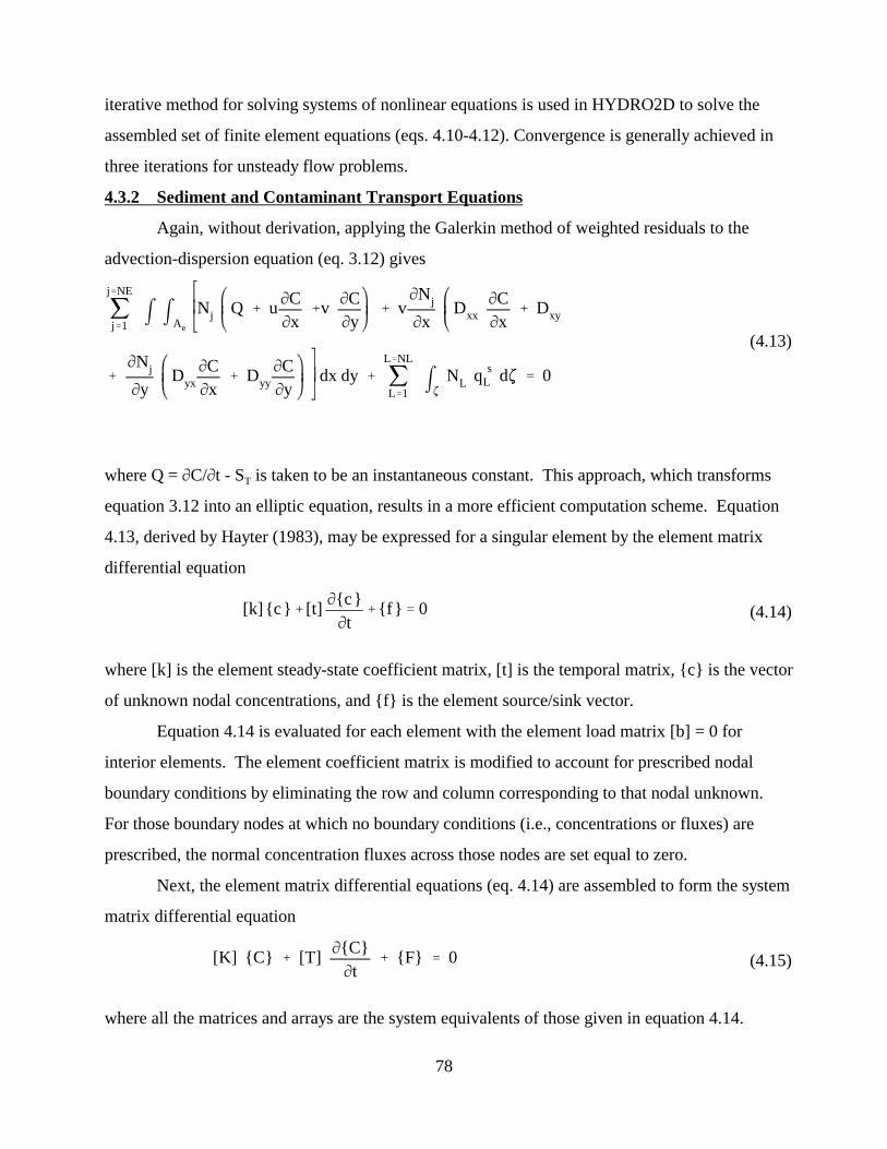
iterative method for solving systems of nonlinear equations is used in HYDRO2D to solve the
assembled set of finite element equations (eqs. 4.10-4.12). Convergence is generally achieved in
three iterations for unsteady flow problems.
4.3.2 Sediment and Contaminant Transport Equations
Again, without derivation, applying the Galerkin method of weighted residuals to the
advection-dispersion equation (eq. 3.12) gives
j'NE MNMC MC MCN Q % u %v % v j D % Dj xx xyj m mA Mx My Mx Mxj'1 e
(4.13) L
j'NLMN MC MC
% j D % D dx dy % m. NL q s d. ' 0Lyx yyMy Mx My L'1
where Q = MC/Mt - ST is taken to be an instantaneous constant. This approach, which transforms
equation 3.12 into an elliptic equation, results in a more efficient computation scheme. Equation
4.13, derived by Hayter (1983), may be expressed for a singular element by the element matrix
differential equation
[k] {c } % [t] M{c }
% {f } ' 0 (4.14)Mt
where [k] is the element steady-state coefficient matrix, [t] is the temporal matrix, {c} is the vector
of unknown nodal concentrations, and {f} is the element source/sink vector.
Equation 4.14 is evaluated for each element with the element load matrix [b] = 0 for
interior elements. The element coefficient matrix is modified to account for prescribed nodal
boundary conditions by eliminating the row and column corresponding to that nodal unknown.
For those boundary nodes at which no boundary conditions (i.e., concentrations or fluxes) are
prescribed, the normal concentration fluxes across those nodes are set equal to zero.
Next, the element matrix differential equations (eq. 4.14) are assembled to form the system
matrix differential equation
[K] {C} % [T] M{C}
% {F} ' 0 (4.15)Mt
where all the matrices and arrays are the system equivalents of those given in equation 4.14.
78
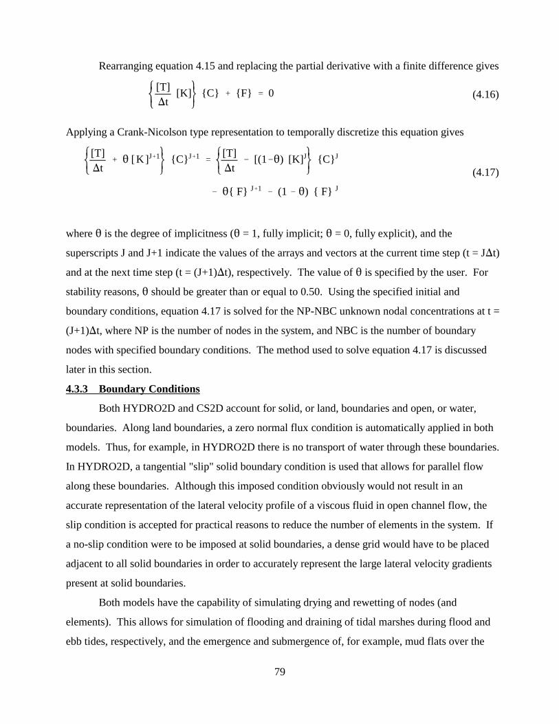
[T] )t
[K] {C} % {F} ' 0 (4.16)
Applying a Crank-Nicolson type representation to temporally discretize this equation gives
[T] )t
% 2 [K ]J%1 {C}J%1 ' [T] )t
& [(1&2) [K]J {C}J
(4.17)
& 2{ F} J%1 & (1 & 2) { F} J
Rearranging equation 4.15 and replacing the partial derivative with a finite difference gives
where 2 is the degree of implicitness (2 = 1, fully implicit; 2 = 0, fully explicit), and the
superscripts J and J+1 indicate the values of the arrays and vectors at the current time step (t = J)t)
and at the next time step (t = (J+1))t), respectively. The value of 2 is specified by the user. For
stability reasons, 2 should be greater than or equal to 0.50. Using the specified initial and
boundary conditions, equation 4.17 is solved for the NP-NBC unknown nodal concentrations at t =
(J+1))t, where NP is the number of nodes in the system, and NBC is the number of boundary
nodes with specified boundary conditions. The method used to solve equation 4.17 is discussed
later in this section.
4.3.3 Boundary Conditions
Both HYDRO2D and CS2D account for solid, or land, boundaries and open, or water,
boundaries. Along land boundaries, a zero normal flux condition is automatically applied in both
models. Thus, for example, in HYDRO2D there is no transport of water through these boundaries.
In HYDRO2D, a tangential "slip" solid boundary condition is used that allows for parallel flow
along these boundaries. Although this imposed condition obviously would not result in an
accurate representation of the lateral velocity profile of a viscous fluid in open channel flow, the
slip condition is accepted for practical reasons to reduce the number of elements in the system. If
a no-slip condition were to be imposed at solid boundaries, a dense grid would have to be placed
adjacent to all solid boundaries in order to accurately represent the large lateral velocity gradients
present at solid boundaries.
Both models have the capability of simulating drying and rewetting of nodes (and
elements). This allows for simulation of flooding and draining of tidal marshes during flood and
ebb tides, respectively, and the emergence and submergence of, for example, mud flats over the
79

course of a tidal cycle.
The open or water boundary conditions that have to be specified in HYDRO2D are either
the water surface elevations or unit discharges at all nodes across the boundary. The depth-
averaged suspension concentrations have to be specified at open boundary nodes in HSCTM-2D or
zero concentration gradients are automatically applied to those boundary nodes.
4.3.4 Equations Solver
The finite element modeling system HSCTM-2D uses the frontal solution program for
unsymmetric matrices developed by Hood (1976) to solve the assembled systems of finite element
equations. The frontal algorithm was developed specifically for applications to boundary value
problems. Although it is based on the Gaussian elimination technique, it has advantages over
conventional banded matrix techniques in that computer storage requirements and computation
times may be considerably reduced in certain applications.
80
SECTION 5
DESCRIPTION OF THE MODELING SYSTEM
5.1 SYSTEM COMPONENTS
The finite element modeling system HSCTM-2D, a flowchart of which is given in Figure
1.1, is a set of computer programs written in FORTRAN 77 that have been integrated into a single
package for modeling two-dimensional, depth-averaged surface water flows and transport of
cohesive sediments. The programs are a hydrodynamic model, HYDRO2D, and a cohesive
sediment transport model, CS2D. SMS, obtained separately, is used for pre- and post-processing.
The modeling system can be operated in either an uncoupled or semi-coupled mode (see
Figure 1.1). In the former, HYDRO2D is used to specify the nodal water depths and velocities for
the entire period of simulation and then CS2D solves for the spatial and temporal variations in the
suspension concentration and bed surface elevations using the output from HYDRO2D. Operated
in the semi-coupled mode, the modeling system runs both models during the first time step, CS2D
at all subsequent time steps, and HYDRO2D at specified time steps. The semi-coupled mode
allows predicted changes in flow depths resulting from deposition and erosion to be incorporated
in the predicted flow field.
The following two subsections describe the structure of the two computer programs
included in the HSCTM-2D modeling system. A detailed description of the algorithms included in
HSCTM-2D, which simulate the processes of erosion, dispersion, and deposition, are given in
Section 5.3. A description of the default option of the HSCTM-2D is given in Section 8.6.
81
5.2 HYDRODYNAMIC MODULE
The hydrodynamic module HYDRO2D simulates two-dimensional, depth-averaged flow of
surface waters. The governing equations, eqs. 3.1, 3.7 and 3.8, are solved by the Galerkin method
of weighted residuals using the finite element method, as described in Section 4. The depth-
averaged velocities in the two horizontal directions and the flow depth are computed at each node.
In addition, continuity can be checked across multiple cross-sections. The effects of bottom,
internal, and surface shear stresses and the Coriolis force are simulated in HYDRO2D. Bottom
and surface stresses are due to friction; internal stresses are the results of turbulence.
The module can simulate both steady state and dynamic flows. Boundary conditions at
system "water" boundaries may be specified as either (a) the total discharge across the boundary in
a specified direction, (b) the water surface elevation along the boundary, or (c) as a stage-discharge
relationship. The data input routine in HYDRO2D reads the output (finite element grid) file
generated by SMS. HYDRO2D has the ability to handle drying and wetting of nodes, thus
simulating emergence and/or submergence of a particular portion of the water system, e.g., mud
flats, over a tidal cycle. User instructions and a brief description of the function of each subroutine
in HYDRO2D are included in Section 8. A synopsis of the operations performed during model
operation is given below.
After the input data file is read, the finite element grid is examined for compatibility (with
dimensioned arrays) and consistency (of node and element order). The system of finite element
equations is established and then solved by the frontal elimination method. Newton's method is
used to obtain an iterative solution of the nonlinear finite element equations by multiple calls to
the frontal routine. The results are printed out after the specified number of iterations. For
dynamic (time-dependent) problems, boundary conditions are updated at each time-step.
5.3 COHESIVE SEDIMENT TRANSPORT MODEL
The cohesive sediment transport model CS2D is a time varying, two-dimensional finite
element model that is capable of predicting the horizontal and temporal variations in the depth-
averaged suspended cohesive sediment concentrations and bed surface elevations in an estuary,
coastal waterway or river (Hayter and Mehta 1986). In addition, it can be used to predict the
steady-state or unsteady transport of any conservative or non-conservative constituent if the
82
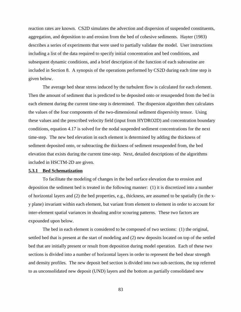
reaction rates are known. CS2D simulates the advection and dispersion of suspended constituents,
aggregation, and deposition to and erosion from the bed of cohesive sediments. Hayter (1983)
describes a series of experiments that were used to partially validate the model. User instructions
including a list of the data required to specify initial concentration and bed conditions, and
subsequent dynamic conditions, and a brief description of the function of each subroutine are
included in Section 8. A synopsis of the operations performed by CS2D during each time step is
given below.
The average bed shear stress induced by the turbulent flow is calculated for each element.
Then the amount of sediment that is predicted to be deposited onto or resuspended from the bed in
each element during the current time-step is determined. The dispersion algorithm then calculates
the values of the four components of the two-dimensional sediment dispersivity tensor. Using
these values and the prescribed velocity field (input from HYDRO2D) and concentration boundary
conditions, equation 4.17 is solved for the nodal suspended sediment concentrations for the next
time-step. The new bed elevation in each element is determined by adding the thickness of
sediment deposited onto, or subtracting the thickness of sediment resuspended from, the bed
elevation that exists during the current time-step. Next, detailed descriptions of the algorithms
included in HSCTM-2D are given.
5.3.1 Bed Schematization
To facilitate the modeling of changes in the bed surface elevation due to erosion and
deposition the sediment bed is treated in the following manner: (1) it is discretized into a number
of horizontal layers and (2) the bed properties, e.g., thickness, are assumed to be spatially (in the x-
y plane) invariant within each element, but variant from element to element in order to account for
inter-element spatial variances in shoaling and/or scouring patterns. These two factors are
expounded upon below.
The bed in each element is considered to be composed of two sections: (1) the original,
settled bed that is present at the start of modeling and (2) new deposits located on top of the settled
bed that are initially present or result from deposition during model operation. Each of these two
sections is divided into a number of horizontal layers in order to represent the bed shear strength
and density profiles. The new deposit bed section is divided into two sub-sections, the top referred
to as unconsolidated new deposit (UND) layers and the bottom as partially consolidated new
83

deposit (PCND) layers (see Figure 5.1). The former sub-section, which represents a stationary
suspension, is considered to undergo redispersion; the latter, i.e., partially consolidated bed,
undergoes resuspension when subjected to an excess shear stress. The settled bed as well is
simulated to resuspend. The number of layers indicated in Figure 5.1 for each of the three bed
sections are not fixed, as each section can be assigned any number of layers.
Stationary suspensions are represented in the depth-averaged model as being the top
section of the layered bed model, even though they are not a true bed or soil, in order to account
for the subsequent redispersion of these suspensions. The time-varying bed thickness in each
element, however, is taken to be equal to the thickness of the PCND layers and settled bed layers
only. The following bed-related parameters are required for bed schematization:
1) The bed shear strength, Jc, profile of a stationary suspension. This can be
ascertained from laboratory erosion tests using samples of sediment from the water
body being modeled (see Section 6.1). The Jc values at the NLAYTM+1 nodes,
where NLAYTM is the number of UND layers, (see Figure 5.2) need to be included
in the data input file.
2) The number of UND layers (NLAYTM) and the thickness of each layer
(TLAYM(I), I= 1,NLAYTM). These parameters should be determined using the
shear strength profile. For example, Figure 5.2 shows a hypothetical Jc profile and
illustrates how this bed section should be divided such that the variation of Jc
within each layer is approximately linear.
3) The dry sediment density, Ds, values at the NLAYTM+1 nodes. The Ds profiles may
be determined using the laboratory freeze-drying method described by Parchure
(1980), the pumping method described by Thorn and Parsons (1977), a gamma-ray
nuclear transmission densitometer (Whitmarsh 1971), or a nondestructive X-ray
technique (Been and Sills 1981).
84
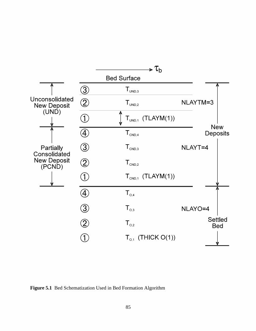
Figure 5.1 Bed Schematization Used in Bed Formation Algorithm
85
Figure 5.2 Hypothetical Shear Strength Profile Illustrating Determination of Bed Layer Thickness.
4) The corresponding parameters as in steps 1 to 3 above must be determined for the
PCND layers and the settled bed layers. The settled bed parameters have to be
determined for each element (where an original bed exists), but the parameters for
the UND and PCND layers are assumed to be constants for all elements.
5) A stationary suspension and/or partially consolidated bed (i.e., new deposit) present
on top of the settled bed at the start of the modeling is simulated by specifying the
dry sediment mass per unit bed area of such new deposits in every element.
The bed level at which the dry sediment density is approximately 480 kg/m3 is usually
taken to be the top of the settled bed. Thus, the sediments located above this level are considered
to be new deposits. Another method that may be used to differentiate between new deposits and
the settled bed is described in Section 6.1.
86
Included in Section 6.1 is a brief description of how these various bed properties can be
determined through the use of a field data collection program and a laboratory testing program.
Other parameters characterizing the rate of resuspension that each layer undergoes when subjected
to an excess shear must be evaluated as well; these are discussed in Section 5.3.2.
The following procedure is used to form the new deposit bed layer(s) that result from new
deposits initially present on top of the settled bed and/or deposited during modeling. The dry
sediment mass per unit bed area per element, MD, either the initial amount or the amount deposited
during modeling, is used in conjunction with the UND and PCND properties to solve iteratively
for the thickness of the bed formed for each element where MD > 0. This thickness, )T, depends
on the dry sediment density profile, Ds(Z), for the UND and PCND layers, where Z is the
coordinate that defines the depth below the bed surface. The thickness )T is determined using the
following relationship:
8
m0 D (Z) Z dZ s
)T ' (5.1) MD
where 8 = )T ± 0.02)T. If )T is greater than TLAYM(1) (see Figure 5.1), then more than one
layer of UND is added. The assumed linear variation of Ds within each layer is used in the above
equation. When the UND layers are filled, the same procedure is used to fill up the PCND layers
below the UND layers. The bottom PCND layer can never completely fill up; therefore,
continuing deposition is accounted for by increasing the thickness of this layer, while the thickness
of the overlying UND and PCND layers remain the same.
5.3.2 Erosion Algorithm
A description of the redispersion and resuspension algorithms is given below. In both
algorithms, the rate of erosion is calculated on an element by element basis.
A portion of the unconsolidated new deposit (UND), when present, will redisperse (mass
erode) when Jb is greater than the surface shear strength, i.e., Jc(Z=0). The thickness of the UND
that fails and is instantly redispersed is equal to Z*, where Z* is the bed depth at which Jc(Z) = Jb.
The value of Z* is determined from the linearly varying Jc(zb) profile in each UND layer. The
value of Z* may be greater than the thickness of the top layer, TLAYM(1), in which case more than
87
one layer is re-entrained. The sediment mass per unit bed area that is redispersed, MR, during one
time-step, )T, is calculated according to
MR ' m0
Z( D (Z) dz s (5.2)
The contribution to the source term in the governing equation (eq. 3.12) caused by redispersion is
given by MR divided by the product of the element-averaged water depth and time-step size )t.
New UND layer(s) thicknesses and Jc(Z) and Ds(Z) profiles are calculated at each time-step when
redispersion occurs by subtracting Z* and resetting Jc(Z=0) and Ds(Z=0) equal to their respective
initial values at Z = Z*. If Z* is calculated to be greater than the thickness of the entire UND, then
all of the stationary suspension is redispersed.
For both redispersion and resuspension algorithms, erosion is considered to occur only
during accelerating flows, i.e., Jb(t+)t) > Jb(t). Thus, even though Jb(t+)t) may be greater than
Jc(Z=0), no erosion will occur if Jb(t) > Jb(t+)t). This stipulation for occurrence of erosion and an
analogous one for deposition (as will be discussed in Section 5.3.4), are based on an interpretation
of typically observed Eulerian time-concentration profiles in an estuarial environment. For
example, Figure 3.3 shows a time-concentration profile from the Savannah River estuary (Krone
1972). Also indicated is the observed correlation between accelerating flows and increasing
suspension concentration, and between decelerating flows and decreasing suspension
concentration. Laboratory evidence (Mehta and Partheniades 1975; Partheniades 1977; Mehta et
al. 1982a; Parchure 1984) suggests that under accelerating flows, erosion occurs without re-
deposition of the eroded sediment. Likewise, during decelerating flows, sediment is deposited
with re-entrainment of the deposit. During periods of steady flows, erosion or deposition may
occur. These two processes do not, however, occur simultaneously (except as noted below) even
in this case (Parchure 1984). The initial condition at the inception of the steady flow period
determines whether erosion or deposition occurs. For example, if the antecedent phase was one of
acceleration, the sediment will continue to erode under the steady flow condition. In both cases,
however, relatively short transient periods of simultaneous erosion and deposition sometimes
occur (Yeh 1979). For modeling purposes, however, these periods are ignored without introducing
any significant errors.
88
Resuspension of partially consolidated beds (PCND) occurs when: (1) the entire UND has
been redispersed, (2) Jb(t+)t)> Jb(t) and (3) Jb(t+)t) > Jc(Z=0), where Z=0 is now at the water-
PCND interface. The resuspension rate expression (eq. 3.11) found by Mehta et al. (1982a) is
used in the manner shown below to determine the bed thickness Z* that is resuspended during one
time-step, )t. The iterative procedure used to calculate Z* during any given time-step is described
by Hayter (1983).
The average erosion rate, ¯ g , for the period )t is calculated as:
¯ g ' 1 g (t) % g (t % )t) (5.3)2
in which
Jb(t % )t) g (t % )t) ' go1
exp " & 1 (5.4)1 J c
where go1 and " 1 are the average empirical coefficients for the first (i.e., top) PCND layer, and J c
is the average bed strength over Z*. As in the redispersion routine, new PCND layer thickness(es)
and Jc(Z), and Ds(Z) profiles are determined. As before, Z* may be greater than the thickness on
the top layer. Laboratory tests required to evaluate Jc(Z), Ds(Z), and the average values of go and "
for each PCND layer are described in Section 6.1. Values for go and " reported in the literature are
given in Table 5.1.
Once the entire new deposit bed section has been eroded, the original settled bed will
undergo resuspension when the following two conditions occur: 1) Jb(t+)t) > Jb(t) and 2) Jb(t+)t)
> Jc(Z=0), where Z=0 is now at the top of the settled bed. The surface erosion rate expression (eq.
3.10) given by Ariathurai and Arulanandan (1978) is used to evaluate the thickness, Z*, of the
settled bed that is eroded during each time-step. The iterative procedure used for the PCND is
again used to solve for Z*, with only the expression for g being different. The following equation
is used instead of equation 5.4.
89
Jb(t % )t) g (t % )t) ' M(1) & 1 (5.5)
J c
where M(1) is the erodibility constant for the first layer. Values for M reported in the literature are
listed in Table 5.1.
The contribution to the source term in equation 3.12 caused by resuspension is given by
equation 5.3 divided by the average elemental water depth, with equation 5.4 used for the partially
consolidated bed section and equation 5.5 used for the original settled bed section.
The bed shear strength profiles, shown in Figure 3.5, were analyzed by determining the
weighted depth-averaged value (weighted with respect to spacing, i.e., depth, among adjacent data
points) of J at the five different salt concentrations, S. The following relationship was found: c
SJ (S) ' % 1 @ J c for 0 # S < 2 c (S ' 0)2 (5.6)
J (S) ' 2 @ J c for S $ 2 c (S ' 0)
where S is in ppt. The method used to include the effect of salinity on bed shear strength profiles,
and hence on the erosion rate of that bed is described by Hayter (1983).
5.3.3 Dispersion Algorithm
The most important, and possibly the most difficult, task in modeling dispersion is to
determine which of the dispersion mechanisms are important in the water body being modeled.
For example, if the estuary has only a few tidal flats and shore irregularities, and has a fairly
uniform cross-section (e.g., the Delaware River), shear flow dispersion may be the dominant
mechanism. However, if the estuary is relatively deep and the river discharge is large (e.g., the
Mississippi River), gravitational circulation may be just as (or even more) important than shear
flow dispersion. Unfortunately, none of the existing dispersion models, most of which
90
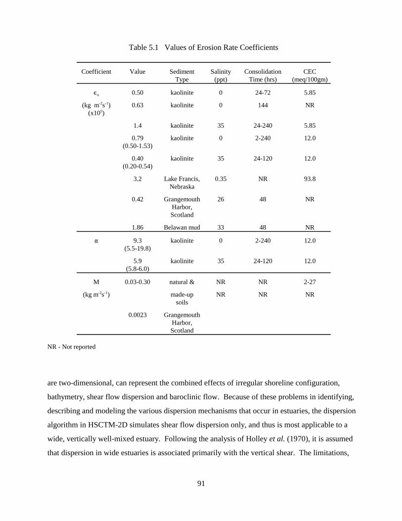
Table 5.1 Values of Erosion Rate Coefficients
Coefficient Value Sediment Salinity Consolidation CEC Type (ppt) Time (hrs) (meq/100gm)
,o 0.50 kaolinite 0 24-72 5.85
(kg m-2s-1) 0.63 kaolinite 0 144 NR (x105)
1.4 kaolinite 35 24-240 5.85
0.79 kaolinite 0 2-240 12.0 (0.50-1.53)
0.40 kaolinite 35 24-120 12.0 (0.20-0.54)
3.2 Lake Francis, 0.35 NR 93.8 Nebraska
0.42 Grangemouth 26 48 NR Harbor, Scotland
1.86 Belawan mud 33 48 NR
" 9.3 kaolinite 0 2-240 12.0 (5.5-19.8)
5.9 kaolinite 35 24-120 12.0 (5.8-6.0)
M 0.03-0.30 natural & NR NR 2-27
(kg m-2s-1) made-up NR NR NR soils
0.0023 Grangemouth Harbor, Scotland
NR - Not reported
are two-dimensional, can represent the combined effects of irregular shoreline configuration,
bathymetry, shear flow dispersion and baroclinic flow. Because of these problems in identifying,
describing and modeling the various dispersion mechanisms that occur in estuaries, the dispersion
algorithm in HSCTM-2D simulates shear flow dispersion only, and thus is most applicable to a
wide, vertically well-mixed estuary. Following the analysis of Holley et al. (1970), it is assumed
that dispersion in wide estuaries is associated primarily with the vertical shear. The limitations,
91
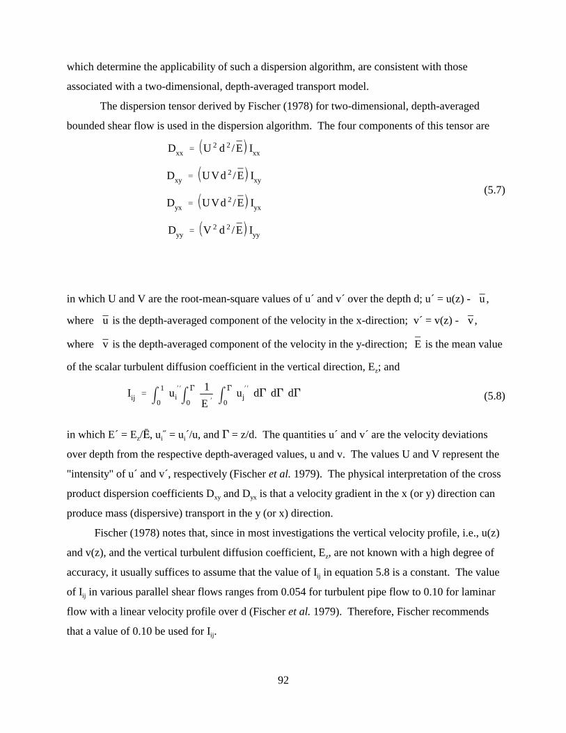
which determine the applicability of such a dispersion algorithm, are consistent with those
associated with a two-dimensional, depth-averaged transport model.
The dispersion tensor derived by Fischer (1978) for two-dimensional, depth-averaged
bounded shear flow is used in the dispersion algorithm. The four components of this tensor are
E I
E I
E I
E I
¯D ' U 2 d 2 / xxxx
¯D ' UVd 2 / xyxy
(5.7) ¯D ' UVd 2 / yxyx
¯D ' V 2 d 2 / yyyy
in which U and V are the root-mean-square values of u´ and v´ over the depth d; u´ = u(z) - , u
where u is the depth-averaged component of the velocity in the x-direction; v´ = v(z) - v ,
¯where v is the depth-averaged component of the velocity in the y-direction; E is the mean value
of the scalar turbulent diffusion coefficient in the vertical direction, Ez; and
' NNIij ' m0
1 ui NN
m0
'
E
1 N m0
uj d' d' d' (5.8)
in which E´ = E /ê, ui1 = ui´/u, and ' = z/d. The quantities u´ and v´ are the velocity deviations z
over depth from the respective depth-averaged values, u and v. The values U and V represent the
"intensity" of u´ and v´, respectively (Fischer et al. 1979). The physical interpretation of the cross
product dispersion coefficients Dxy and Dyx is that a velocity gradient in the x (or y) direction can
produce mass (dispersive) transport in the y (or x) direction.
Fischer (1978) notes that, since in most investigations the vertical velocity profile, i.e., u(z)
and v(z), and the vertical turbulent diffusion coefficient, Ez, are not known with a high degree of
accuracy, it usually suffices to assume that the value of Iij in equation 5.8 is a constant. The value
of Iij in various parallel shear flows ranges from 0.054 for turbulent pipe flow to 0.10 for laminar
flow with a linear velocity profile over d (Fischer et al. 1979). Therefore, Fischer recommends
that a value of 0.10 be used for Iij.
92

The following expression for Ez, derived by Elder (1959) for flow down an infinitely wide
inclined plane, is used in this analysis:
E ' 6 uf z 1 & z
(5.9)z d
where 6 is the von Karman turbulence constant, and uf is the shear velocity. Therefore, ê is given
by
¯ 1 d 6 uf d E '
d m0 E dz ' ' 0.067 uf d (5.10)z 6
with 6 = 0.40. The values of 6 obtained by Gust (1976) from the slopes of measured clay
suspension velocity profiles varied between 0.3 and 0.4. Gust considered this variation a result of
experimental error and not due to the presence of suspended sediments. Therefore, he assumed 6
= 0.40 in his analysis.
Fischer (1966) found, in both laboratory experiments and in real streams, that the mean
value of U 2/u 2 was equal to 0.2. Substituting this value, Iij = 0.1, and equation 5.10 into
equation 5.7 gives:
2 d 20.2 u u 2 dD ' (0.10) ' 0.30 xx 0.067uf d uf
0.2uv d 2 uv dD ' (0.10) ' 0.30 xy 0.067uf d uf
(5.11) 0.2uv d 2 uv d
D ' (0.10) ' 0.30 yx 0.067uf d uf
2 d 20.2 v v 2 dD ' (0.10) ' 0.30 yy 0.067 uf d uf
93
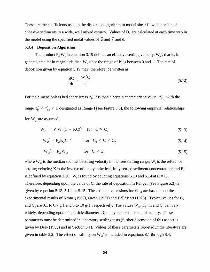
These are the coefficients used in the dispersion algorithm to model shear flow dispersion of
cohesive sediments in a wide, well mixed estuary. Values of Dij are calculated at each time step in
u and ¯the model using the specified nodal values of ¯ v and d.
5.3.4 Deposition Algorithm
The product Pd@Ws in equation 3.19 defines an effective settling velocity, Ws´, that is, in
general, smaller in magnitude than Ws since the range of Pd is between 0 and 1. The rate of
deposition given by equation 3.19 may, therefore, be written as
' dC
' W C s (5.12)
dt d
For the dimensionless bed shear stress J( less than a certain characteristic value, J( , with theb bc
range J( < J( < 1 designated as Range I (see Figure 5.3), the following empirical relationships b bc
' for W are assumed: s
' ' Pd W (1 & KC)5 for C > C2 (5.13)Ws1 r
' ' Pd K C m for C1 < C < C2 (5.14)Ws1 e
' for C < C1 (5.15)Ws1 ' Pd Ws1
where Ws1 is the median sediment settling velocity in the free settling range; Wr is the reference
settling velocity; K is the inverse of the hypothetical, fully settled sediment concentration; and Pd
is defined by equation 3.20. Wr is found by equating equations 5.13 and 5.14 at C = C2.
Therefore, depending upon the value of C, the rate of deposition in Range I (see Figure 5.3) is
given by equation 5.13, 5.14, or 5.15. These three expressions for W´s1 are based upon the
experimental results of Krone (1962), Owen (1971) and Bellessort (1973). Typical values for C1
and C2 are 0.1 to 0.7 g/1 and 5 to 10 g/1, respectively. The values Ws1, Ke, m and C1 can vary
widely, depending upon the particle diameter, D, the type of sediment and salinity. These
parameters must be determined in laboratory settling tests (further discussion of this aspect is
given by Delo (1988) and in Section 6.1). Values of these parameters reported in the literature are
given in table 5.2. The effect of salinity on Ws1' is included in equations 8.1 through 8.4.
94

For J( < J( / and the concentration range C > C1, designated as Range IIB, the bc b < Jbmax Jbmin
rate of deposition is determined using the log-normal relationship derived by Mehta and
Partheniades (1975):
&T 2
(J( & 1)dC '
& 0.434 exp 2.04 b2 (5.16)C 1&erf 2
log10o 4 exp(&1.27Jbmin)dt 2 2BF2t
For J( < 1, the argument of the error function is set equal to zero. Values of deposition rateb
coefficients reported in the literature are included in Table 5.2. Equation 5.16 is assumed to be
valid for C > C1 because the phenomenon of hindered settling was not observed in the steady-state
deposition tests performed by Mehta (1973) for concentrations up to about 20 g/1. Evidently, the
higher J( values Mehta used in his tests prevented the occurrence of this modeb
Figure 5.3 Apparent Settling Velocity Description in Domains Defined by Suspended Sediment Concentration and Bed Shear Stress
95
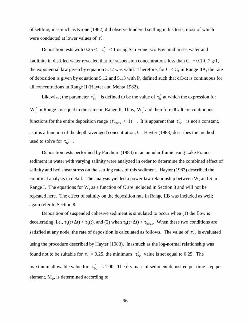
of settling, inasmuch as Krone (1962) did observe hindered settling in his tests, most of which
were conducted at lower values of J( .b
Deposition tests with 0.25 < J( < 1 using San Francisco Bay mud in sea water and b
kaolinite in distilled water revealed that for suspension concentrations less than C1 ï 0.1-0.7 g/1,
the exponential law given by equation 5.12 was valid. Therefore, for C < C1 in Range IIA, the rate
of deposition is given by equations 5.12 and 5.13 with Pd defined such that dC/dt is continuous for
all concentrations in Range II (Hayter and Mehta 1982).
Likewise, the parameter J( is defined to be the value of J( at which the expression for bc b
' ' W in Range I is equal to the same in Range II. Thus, Ws and therefore dC/dt are continuouss
functions for the entire deposition range (J( < 1) . It is apparent that J( is not a constant,bmax bc
as it is a function of the depth-averaged concentration, C. Hayter (1983) describes the method
used to solve for J( .bc
Deposition tests performed by Parchure (1984) in an annular flume using Lake Francis
sediment in water with varying salinity were analyzed in order to determine the combined effect of
salinity and bed shear stress on the settling rates of this sediment. Hayter (1983) described the
empirical analysis in detail. The analysis yielded a power law relationship between Ws and S in
Range I. The equations for Ws as a function of C are included in Section 8 and will not be
repeated here. The effect of salinity on the deposition rate in Range IIB was included as well;
again refer to Section 8.
Deposition of suspended cohesive sediment is simulated to occur when (1) the flow is
decelerating, i.e., Jb(t+)t) < Jb(t), and (2) when Jb(t+)t) < Jbmax. When these two conditions are
satisfied at any node, the rate of deposition is calculated as follows. The value of J( is evaluatedbc
using the procedure described by Hayter (1983). Inasmuch as the log-normal relationship was
found not to be suitable for J( < 0.25, the minimum J( value is set equal to 0.25. Theb bc
maximum allowable value for J( is 1.00. The dry mass of sediment deposited per time-step per bc
element, MD, is determined according to
96
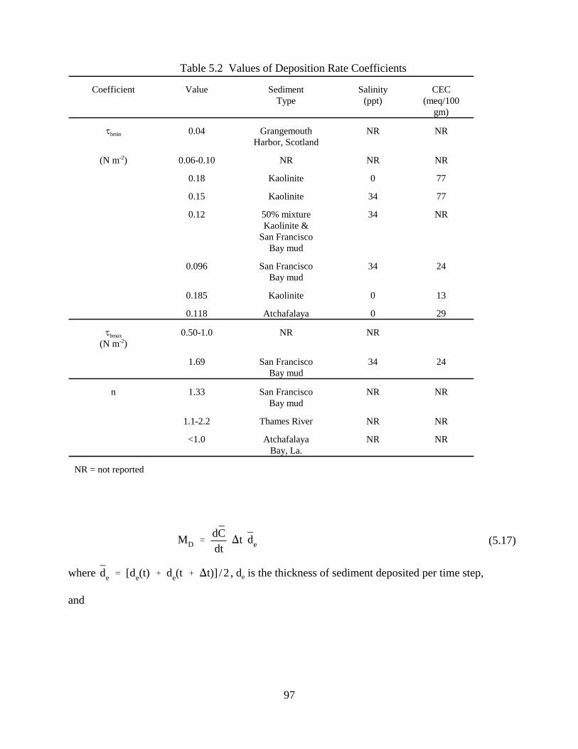
Table 5.2 Values of Deposition Rate Coefficients
Coefficient Value Sediment Salinity CEC Type (ppt) (meq/100
gm)
Jbmin 0.04 Grangemouth NR NR Harbor, Scotland
(N m-2) 0.06-0.10 NR NR NR
0.18 Kaolinite 0 77
0.15 Kaolinite 34 77
0.12 50% mixture 34 NR Kaolinite &
San Francisco Bay mud
0.096 San Francisco 34 24 Bay mud
0.185 Kaolinite 0 13
0.118 Atchafalaya 0 29
Jbmax 0.50-1.0 NR NR (N m-2)
1.69 San Francisco 34 24 Bay mud
n 1.33 San Francisco NR NR Bay mud
1.1-2.2 Thames River NR NR
<1.0 Atchafalaya NR NR Bay, La.
NR = not reported
dCMD ' )t de (5.17)
dt
where d ' [de(t) % d (t % )t)] /2 , de is the thickness of sediment deposited per time step, e e
and
97
dC '
1 dC dC/ % / (5.18)dt 2 dt 00 t dt 00 t%)t
in Range I and Range IIA, and
d¯ ¯ )t 0.434¯C '
C (1&C ( ) erf ln % 1 eq (5.19)dt 4)t ¯ 2B F2t 50
¯in Range IIB. In equation 5.19, 2 ' [2 (t) % 2 (t%)t)] /2 , where 2 = C, t50, C*eq, F2 and J(
. Theb
last term is included because C* is a function of J( . Equation 5.19 was obtained by integration ofeq b
equation 5.16 from t=0 to t=)t. Section 5.3.1 describes the procedure for calculating the bed
thickness formed by MD. The sink term in the governing equation (equation 3.12) is given by
equation 5.18 in Ranges I and IIA, and by equation 5.19 for Range IIB.
Under unsteady flows, the value of Ceq, which is the steady state value of the suspended
sediment concentration found in laboratory deposition tests under steady flows, is assumed to be
zero. Nevertheless, the laboratory determined log-normal relationship for dC/dt, as given by
equation 5.19, is used for Range IIB for the following reasons. The time-step, )t, used in the
estuarial sediment transport problems is typically of the order 0.1 t50 < )t < 10t50. Therefore, dC/dt
(given by equation 5.19 is significantly greater than zero at time )t. This implies that, after any
time interval )t, the suspended sediment concentration, C(t+)t), does not approach Ceq, but is
assumed to be equal to the following:
d¯C(t % )t) ' C( t ) &
C )t (5.20)dt
where dC/dt is given by equation 5.19. Thus, for unsteady flow conditions, the rate of deposition
is considered to be a function of C . Such a consideration is required for a realistic interpretationeq
of deposition results for the purpose of ascertaining the depositional rates in unsteady estuarial
environments.
98
SECTION 6
DATA COLLECTION AND MODEL CALIBRATION
Delo (1988) summarizes procedures that may be used for determination of some of the
empirical coefficients contained in expressions for the rate of sediment transport processes of
erosion and deposition when limited information about field conditions is available. He also
emphasizes that "the behavior of cohesive sediment does vary considerably in quantitative terms
from one source to another. Therefore, it is crucial that the engineer appreciates that estimates
based on the data presented herewith may well be in error by half an order of magnitude (or
more)."
6.1 DATA COLLECTION AND ANALYSIS
6.1.1 Field Data Collection Program
A field data collection program for a sedimentation study should consist of four principal
components: (1) hydrographic survey; (2) sediment sampling; (3) measurement of suspended
sediment concentration, water temperature and salinity; and (4) determination of sediment settling
velocity. The collection program required for modeling the hydrodynamic regime in an estuary is
rather well known and will not be addressed in this report. For one reference, refer to Smoot and
Novak (1969).
6.1.1.1 Hydrographic Survey
At least two sonar fathometers and a gamma-ray transmission densitometer should be used
to measure the depths in the water body to be modeled. First, the entire water body should be
surveyed simultaneously using, for example, a 30-kHz and a 200-kHz fathometer.
99
Parker and Kirby (1977) reported that the sediment-water interfaces of stationary
suspensions in the Severn Estuary, England, were detected by a 200-kHz fathometer but not by a
30-kHz fathometer. In areas where stationary suspensions are determined to exist (by comparison
of the 30-kHz and 200-kHz records), a gamma-ray transmission densitometer or a turbidity meter
should be used to supplement the depth record obtained with the fathometers. A fathometer alone
may not be capable of detecting the surface of stationary suspension for two reasons: (1) The
acoustic detection of a dense suspension depends on the gradient of the bulk density at the surface
of the suspension and not on the magnitude of the density. In mobile suspensions and in newly
formed stationary suspensions, this density gradient is very small, and in most cases the surfaces of
these suspensions will not be detectable. (2) As the stationary suspension undergoes
consolidation, different levels of the suspension may become detectable to fathometers with
different frequencies at different times, which makes the interpretation of such fathometer records
a difficult and uncertain task (Parker and Kirby 1977).
A gamma-ray transmission densitometer obtains in situ measurements of the sediment bulk
density profiles, and can be used, in addition, to determine the thickness of stationary suspensions
and the location (i.e., vertical elevation with respect to geodetic datum) of the top of the settled
bed, at which the bulk density is usually assumed to be 1300 kg/m3. A static cone penetrometer
directly measures penetration resistance and indirectly measures the shear strength of the sediment.
The densitometer has to be calibrated at the beginning and end of survey operations to determine
the relationship between the radiation count rate and sediment density. Calibration is generally
performed using liquids with different densities. The densitometer is penetrated and retracted in
the sediment at a rate of approximately 2 to 3 mm/sec, during which the radiation count rate and
probe penetration depth are continuously recorded. This system has been used from both ships and
submersibles and has the capability of measuring in situ bulk sediment densities up to 1800 kg/m3,
operating in depths up to 3.6 km, and penetrating one to two meters in cohesive sediment
suspensions (Hirst et al. 1975).
There are three methods used to fix the boat position during hydrographic survey:
(1) optical methods, (2) electronic methods, and (3) combined systems. Optical methods include
double horizontal sextant angle and transit line, and theodolite intersections from shore.
Electronic methods include two megahertz systems, microwave systems and range and bearing
100
systems. Combined systems use a theodolite to determine the bearing and a microwave system to
determine the distance. A description of these three methods is given by Ingham (1975) and Dyer
(1979).
6.1.1.2 Sediment Sampling Using Corers
Before the data collection period begins, at least two 10 to 12 cm diameter cores should be
collected at each sampling station. There are four types of corers in common use today: gravity-
corer, piston-corer, vibracorer and box-corer. The cores are used in determining the erosional and
consolidation characteristics of the existing sediment bed.
6.1.1.3 Measurement of Suspended Concentration, Salinity and Temperature
The first item that must be considered is the time period over which data are to be collected
for eventual use in the model. The time period will be contingent upon the desired results from the
modeling effort. In tidal water bodies, data should preferably be collected over a minimum of 15
hours (assuming the tide is semi-diurnal) over three different tidal cycles: spring, mean and neap.
It would be more desirable to have the data collection period span at least one week starting, for
example, on a spring tide and finishing at the subsequent neap tide. The next consideration is the
number of sampling stations and where they should be located in order to adequately monitor the
spatial variations of the concentration of suspended sediment. Stations must be located at all
exterior water boundaries (cross-sections) of the estuarial system to be modeled. The width of the
boundary cross-section and the lateral variability of the depth should be considered when deciding
upon the minimum number of stations to be located laterally across such a boundary. For
example, stations would definitely be located at prominent features such as navigation channels.
Additional stations should be located at all interior confluences and bifurcations, and at as many
other interior locations as possible. It is recognized that the length of the data collection period
and the number of stations are often less than desired due to economic and logistical
considerations.
At each station, the location of the top of the sediment bed with respect to a geodetic or tidal
datum must be determined using the previously described surveying methods. The water
temperature, electrical conductivity (or salinity) and concentration of suspended sediment should
be measured at least once every one-half hour for the duration of the collection period at each of
the sampling stations. These measurements should preferably be made at a minimum of three
101
depths over the vertical: one-half to one meter below the water surface, mid-depth and one-half
meter above the bottom (i.e., top of sediment bed). For locations where the water depth is greater
than about 3 to 4 m, measurements should be made at additional depths over the vertical. Both the
measurement and analysis of water temperature and electrical conductivity data are discussed by
Dyer (1979). A description of various filtration procedures for determining the suspension
concentration gravimetrically is given by Dyer (1979).
There are three general methods used to measure the suspension concentration: (1) water
sampling, (2) optical methods and (3) gamma-ray densitometer measurements.
Water bottles and shipboard pumps are the most common water sampling devices. The NIO
bottle has capacities for 1.25 to 7.1 liters. Other water bottles, such as the Van Dorn bottle, have
capacities of up to 10 liters or more. The NIO bottle consists of a PVC tube open at both ends
with hemispherical bings on spring loaded arms that close each end when struck by a brass
messenger dropped down the support wire (Dyer 1979).
Shipboard pumps are used to pump water samples up to the vessel through an intake tape
mounted on an instrument package. It is recommended that in situ separation of the water and
sediment be performed on the vessel using the filter method (van Rijn 1979).
Instruments for optical determination of the concentration of suspended sediment include
the transmissometer, the nephelometer, and the Secchi disc. Nephelometers are not very practical
for use in estuaries since they are sensitive to very low concentrations only. Secchi discs can be
used to estimate surface values only. Transmissometers, or electro-optical turbidity meters, have
been used successfully to measure vertical turbidity profiles in, among others, the Severn, Maas,
James and Rappahannock estuaries, and in the Upper Chesapeake Bay (Kirby and Parker 1977;
Nichols et al. 1979). These meters can be used to detect both mobile and stationary suspensions as
their operating range is usually 0.25 to 25 g/l. They have a rapid response time (100 Hz), which
allows profiles in 30 m depths to be taken in 15 to 20 seconds.
Both Kirby and Parker (1977) and Nichols et al. (1979) used instrument arrays on which
were mounted a gamma-ray transmission densitometer, at least one electro-optical turbidity meter,
an electromagnetic current meter, a pressure transducer, and a water temperature and a water
temperature and conductivity probe. In general, the optical turbidity meters would be used to
102
record the concentration profile for suspensions up to 25 g/l and the transmission densitometer
used for denser suspensions.
6.1.1.4 Determination of Sediment Settling Velocity
An appropriate method to measure settling velocities is by using an instrument similar to the
sampling tube developed by Owen (1971), in which undisturbed samples of suspended sediments
are collected in situ in their natural state. The settling velocities of the aggregates are determined
immediately thereafter through use of a bottom withdrawal sedimentation test. The major
drawback of an Owen tube is the quiescent condition in the tube during withdrawal. Allersma
(1980) gives a detailed description of an in situ suspended sediment sampler.
6.1.2 Laboratory Testing Program
The following physicochemical sediment and fluid properties should be determined using
the collected sediment cores.
6.1.2.1 Properties of Undisturbed Sediment Cores
A gamma-ray densitometer may be used to determine the sediment density profile in the
undisturbed cores still in the liner tubes as soon after the cores are obtained as possible. A
description of this procedure is given by Whitmarsh (1971) and Kirby and Parker (1974). If this
instrument is not available, the freeze-drying procedure used by Parchure (1980) and Dixit (1982)
or the pumping method used by Thorn and Parsons (1977) may be used to determine the bulk
density profile. The pumping method consists of removing by suction a thin layer, e.g., 3 cm, from
the top of the core. This procedure is repeated, layer by layer, with each layer analyzed to
determine the mean bulk density.
6.1.2.2 Properties of Original Settled Bed
The bulk density and bed shear strength profiles and the erosion rate constant for each layer
need to be determined for the cores. The number of layers and the thickness of each are
determined from the nature of the bed shear strength profile. The erosion rate constant for each
layer and the shear strength profile can be determined, for example, in the rotating cylinder
erodibility testing apparatus described by Sargunam et al. (1973). In order to use this apparatus,
the core sample must be trimmed. The portion of each core that is sufficiently consolidated such
that it can be trimmed and tested in the erosion apparatus may be defined to be the settled bed.
103

The thickness of this portion defines the location of the top of the settled bed. Soft,
unconsolidated portions of each core are assumed to be new deposits.
6.1.2.3 Properties of New Deposits
For cores with soft, unconsolidated or partially consolidated sediment on top of the settled
portion, the following method may be used to estimate the erosional and depositional
characteristics of such new deposits. The new deposit samples from the cores at all the stations
should be mixed and subjected to laboratory erosion and deposition tests described by Parchure
(1980), Mehta and Partheniades (1973) and Hayter (1983) to determine: the settling velocity as a
function of suspension concentration and salinity; the minimum and maximum depositional shear
stresses Jbmin and Jbmax; the variation of t50 and F2 with the bed shear stress Jb; the number of
characteristic stationary suspension layers, and the thickness, dry sediment density and shear
strength of each layer; the number of characteristic partially consolidated new deposit layers, and
the thickness, dry sediment density, shear strength and resuspension parameters go and " for each
layer; and the variation of the bed shear strength J with Ds. The variation of the bed density and c
shear strength profiles with salinity can be determined by performing the erosion tests at several
salinities between 0 and 35 ppt. The relationship between D and J also needs to be determineds c
for the collected sediment samples. Both the bed shear strength and density profiles may be
determined using the methodology described by Mehta et al. (1982a). These profiles can then be
used to establish an empirical relationship between D and J .s c
6.1.2.4 Aggregate Shear Strength and Density
The determination of the aggregate shear strength, Js, and the aggregate density, Da,
corresponding to each sediment-fluid mixture can be carried out through rheological diagrams of
applied shear stress versus shearing rate (Krone 1963). An example of such a diagram is presented
in Figure 6.1, with shear stress, Js, proportional to the dial reading on the viscometer and shearing
rate proportional to the rotation rate of the outer cylinder of the viscometer. The mixture was
stirred occasionally to offset the effects of settling during the experiment. On Figure 6.1, mixing is
indicated by a change of symbol.
The number of aggregation orders possible for a suspension of a given sediment is equal to
the number of linear segments on the rheological diagram with different slopes. Thus, in Figure
6.1 the sediment sample has two possible orders of aggregation. Each order of aggregation
104
corresponds to a given volume fraction of aggregates (volume occupied by the aggregates divided
by the total volume of the suspension) that in turn can be shown to be related to the relative
differential viscosity (the viscosity of the suspension divided by the viscosity of the suspended
medium). Given the viscosity of the suspending medium, the relative differential viscosity is
determined from the slope of the rheological diagram, and hence the volume fraction can be
calculated. The density, Da, is then computed from the volume fraction.
Krone (1978) postulated that each segment is related to a particular volume fraction and
therefore to a different manner in which the sediment can aggregate, i.e., different order of
aggregation. In addition, he found that as the order of aggregation increases, the interaggregate
pore volume increases and the strength of these aggregates decreases because of limited bonding
area among the lower order aggregates.
6.1.2.5 Fluid Composition
The pH, total salt concentration, and concentrations of ions such as Na+, Ca2+, Mg2+, K+, Fe3+
and C1- should be determined for both the pore fluid in the consolidated bed portion of one core
and a sample of the suspending fluid.
6.1.2.6 Composition and Cation Exchange Capacity of the Sediment
The sediment contained in the consolidated bed portion of one core from each collection
station should be thoroughly mixed so that a spatially homogeneous sample is obtained. A
standard hydrometer analysis should be conducted on each co-prepared sample to determine the
sediment particle size distribution and thereby the percentage by weight of clay, silt and fine to
coarse in each sample. In preparing the samples for this analysis, the sediment must not be
initially air-dried (to obtain the dry weight of the material used in the test), as it has been found
that dried sediment will not completely redisperse when the dispersing agent is added (Krone
1962). For this reason, the total dry weight of the sample must be obtained after the test by
evaporating off all the water in an oven set at approximately 50oC. The percentage of organic
matter by weight should be determined through use of a method such as the Walkley-Black test
(Allison 1965). In addition, it is recommended that X-ray diffraction analysis of the bulk sample,
and < 2 µm unglycolated and glycolated portions be conducted in order to determine the
predominant clay and non-clay mineral constituents. Finally, the cation exchange capacity must be
determined for each sample.
105

Figure 6.1 A Plot of Raw Viscometer Data Obtained from the U.S. Army Corps of Engineers Philadelphia District Sample (after Krone 1963).
6.2 MODEL CALIBRATION
Calibration of the HSCTM-2D modeling system is a two-step process involving first,
calibration of the flow module HYDRO2D, and secondly, the sediment transport module CS2D.
General guidelines are discussed below. While not comprehensive, the recommended procedures
will provide the model user with sufficient background to initiate the first few iterations in the
calibration process. Later iterations are often more site specific in nature.
6.2.1 Hydrodynamic Module
Calibration of the module HYDRO2D involves adjustments of the various internal and
external frictional coefficients until a satisfactory match between model results and measured
velocities and water surface elevations is obtained. This usually requires several runs of the
module with different values of the eddy viscosity coefficient tensor for the internal frictional
forces and the Chezy coefficient and wind shear coefficient for the external frictional stress at the
bottom and water surface, respectively. Even for an experienced modeler, calibration will usually
106
require several iterations. Experience gained by this process will enable the modeler to at least
qualitatively anticipate the effect of coefficient(s) adjustment(s) on module response. This should
result in a reduction in the number of runs required to achieve calibration in future applications of
the modeling system.
6.2.2 Sediment Transport Module
Calibration of the module CS2D, if necessary, may be accomplished through adjustment of
the sediment dispersivity tensor, or more directly by adjustment of one of the coefficients in the
sediment settling velocity model for shoaling problems or one of the coefficients in the erosion
rate expressions for scour problems. The model should first be run using the built-in dispersion
algorithm to calculate the dispersivity tensor and the coefficients in the deposition and erosion
algorithms determined using the tests described in Section 6.1. Then, if necessary, the values of
the appropriate coefficient(s) can be changed until a satisfactory match between model results and,
for example, known shoaling rates is obtained. Again, this in general will require several runs of
the model.
107

SECTION 7
HSCTM-2D USER INSTRUCTIONS
The user must be prepared to undertake the following four essential tasks -- (1) field
measurements, (2) laboratory testing of sediment, (3) numerical modeling of hydrodynamics and
sediment and contaminant transport, and (4) analyses of modeling system simulations -- when
using HSCTM-2D to model a system. Brief discussions of the first two items are given in Section
6.1. Calibration of the modeling system is discussed in Section 6.2, and a description of the output
from the modeling system is given in Section 7.4.
7.1 MODELING SYSTEM LIMITATIONS
A two-dimensional, depth-averaged modeling system such as HSCTM-2D can strictly be
applied only to surface bodies of water, e.g., estuaries, harbors and basins (such as marinas), where
the horizontal dimensions of the water body are at least one order of magnitude greater than the
vertical dimension. Applications to partially mixed water bodies, especially highly stratified water
bodies, should be made when only rough estimates of some sedimentary process (e.g., shoaling
rate) are required.
Currently HSCTM-2D has the capability of simulating the transport and fate of only four
constituents: salinity, one representative size or fraction of cohesionless sediment, one size fraction
of cohesive sediment, and one inorganic contaminant. It is possible, however, to modify the model
so that a greater number of constituents may be included.
Limitations of the numerical modeling system described herein come from four sources: (1)
insufficient data, (2) poor quality data, (3) limitations of our understanding and representations of
108

processes such as dispersion, sediment erosion and deposition, and adsorption/desorption of
contaminants, and (4) limitations of the numerical scheme used to solve the governing equations.
The first two sources are attributed to the fact that, owing mainly to time and cost considerations,
all the bathymetric, hydraulic, sediment and contaminant data required for use in a model such as
CS2D are rarely, if ever, measured and/or collected in the body of water being modeled. In
addition, the quality of the data is often questionable. Data requirements and the field collection
and laboratory testing programs required to obtain these data are described in Section 6.1. The
third and fourth categories are self explanatory. All these limitations are possessed by most
numerical models.
The importance of experience in effectively using numerical models cannot be over
emphasized. Experience gained through knowledge of the physical systems being modeled and
repeated applications of the model will enhance the user's ability to choose the proper values of the
various parameters, e.g., time-step size. The user will also gain the ability to anticipate the effect
of changing the value of a particular parameter by a certain percentage on the model solution (i.e.,
model sensitivity).
7.1.1 Limitations of the Hydrodynamic Module
In addition to the previously mentioned limitation of two-dimensional, vertically averaged
homogeneous flow, the hydrodynamic module HYDRO2D has the following additional
limitations.
C The module will not accurately simulate supercritical flow.
C The model is based on a streamwise bottom slope that is mild and not steeper than (-1:10).
The following guidelines/recommendations should be following in using HYDRO2D.
C For stability, the mesh should be constructed with less than a 20% depth change among
adjacent nodes.
C Set up boundary conditions where accurate data, sufficiently far away from the area of
interest, are available.
C Elements that alternate between wetting and drying may be included. Note that if any of the
nodes attached to an element is dry, the entire element is classified as dry. To maintain
stability of the model, mesh boundaries paralleling flow lines where wetting and drying are
expected to occur is recommended.
109
C The computed results should be compared to measured field data whenever possible.
7.2 USER INSTRUCTIONS
HSCTM-2D requires several files to operate. Two of them, a geometry file describing the
mesh and a boundary condition file, can be generated by using SMS. The other files are described
in Section 8.4.
The model includes two options for data specification: a default option in which default
values (included in the program) are used for specified parameters and a non-default option in
which all data must be specified by the user. The default option is of benefit when, due to
insufficient data, all the required sediment related parameters (e.g., erosion/deposition rate
coefficients) are not available to the modeling system user. As emphasized in this document, the
default option should be used for qualitative analysis only. It will allow the user to make relative
comparisons among various sites or designs. In creating the required input data files, the user
should follow closely the data input instructions for both HYDRO2D and CS2D given in Sections
8.3 and 8.4. Sample input data sets included in Section 9 will assist the user in establishing these
data files. The data sets accompanying the modeling system should be used to assist in
constructing new data sets.
As indicated in Section 7.3, the HSCTM-2D modeling system may be operated in two
different modes: (1) an uncoupled mode, in which first HYDRO2D is run to generate the flow
field, and then CS2D is run to stimulate the sediment/contaminant transport, and (2) a semi-
coupled mode, in which both models are operated in a semi-coupled manner in order to account
for the effect of, for example, extensive sedimentation or scouring on the flow field. The first
example problem described in Section 9 was run in the semi-coupled non-default mode, while the
second was run using the uncoupled mode.
SMS can be employed for post-processing after HSCTM-2D is used to perform the
hydrodynamic and sediment/contaminant transport analysis. HSCTM-2D outputs several
"solution files" containing nodal water surface elevations and flow velocities, nodal suspended
sediment concentrations, nodal bed elevation changes, nodal particulate contaminant
concentrations on the surficial bed sediments, and residual error at each node of the mesh. These
110
solution files can be input by SMS to generate vector plots, color-shaded contour plots, and time-
history diagrams.
7.3 DATA INPUT FOR MAIN PROGRAM OF HSCTM-2D
The format for the data input is given in Section 8.
7.4 SYSTEM DATA OUTPUT
7.4.1 Hydrodynamic Module
Output from the module HYDRO2D consists of the following: program control parameters;
eddy viscosity coefficient; nodal connections and area for each element; (x, y) coordinates, bottom
elevation, network slope, flow and water surface elevation boundary conditions, and the initial
water depth at each node; initial nodal flow velocities, depth and water surface elevations; and
nodal flow velocities, depth and water surface elevation at subsequent time steps. The node and
element data and the initial conditions are optional output. Control for output printing is specified
by the parameter IPRT (see Section 8). Specified output data may be stored on a disk file for use
in CS2D if the modeling system is run in the uncoupled mode or stored on a disk file for use in the
velocity vector plotting routine in SMS. An example of typical output for the semi-coupled mode
is included in Section 9.
7.4.2 Sediment Transport Module
Output from the sediment transport modules in HSCTM-2D consists of the following data:
sediment depositional properties; properties of unconsolidated new deposits, partially consolidated
new deposits and the original settled bed; and initial nodal flow velocities, depths, suspension
concentrations, and sediment dispersivity coefficients. Additional information can be obtained at
specified time steps and for specified elements. At specified time steps, the output consists of: the
nodal suspension concentrations, elemental bed shear stresses, bottom elevations, erosion and
deposition rates and properties (e.g., layer thickness, average shear strength, and bulk and dry
density) of all bed sections present in each element. The data printed at specified time steps (i.e.,
when IFF(I,2) > 0; see Section 9) are chosen by the value of IFF(I,2), where I is the time step
number. Specified output data (e.g., nodal suspension concentrations, change in nodal bed
elevations) are stored on disk files for use by the contour plotting routine in SMS. For specified
111
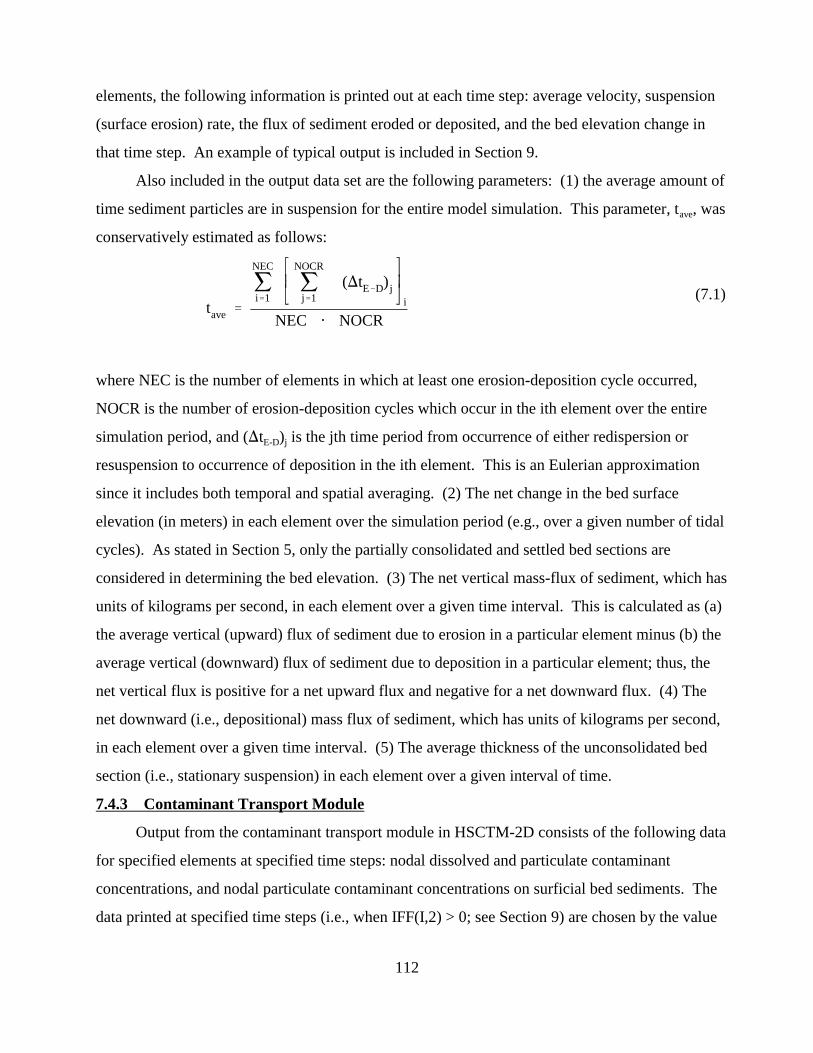
elements, the following information is printed out at each time step: average velocity, suspension
(surface erosion) rate, the flux of sediment eroded or deposited, and the bed elevation change in
that time step. An example of typical output is included in Section 9.
Also included in the output data set are the following parameters: (1) the average amount of
time sediment particles are in suspension for the entire model simulation. This parameter, tave, was
conservatively estimated as follows:
NEC NOCR
j j ()tE&D)j (7.1)i'1 j'1 it ' ave NEC @ NOCR
where NEC is the number of elements in which at least one erosion-deposition cycle occurred,
NOCR is the number of erosion-deposition cycles which occur in the ith element over the entire
simulation period, and ()tE-D)j is the jth time period from occurrence of either redispersion or
resuspension to occurrence of deposition in the ith element. This is an Eulerian approximation
since it includes both temporal and spatial averaging. (2) The net change in the bed surface
elevation (in meters) in each element over the simulation period (e.g., over a given number of tidal
cycles). As stated in Section 5, only the partially consolidated and settled bed sections are
considered in determining the bed elevation. (3) The net vertical mass-flux of sediment, which has
units of kilograms per second, in each element over a given time interval. This is calculated as (a)
the average vertical (upward) flux of sediment due to erosion in a particular element minus (b) the
average vertical (downward) flux of sediment due to deposition in a particular element; thus, the
net vertical flux is positive for a net upward flux and negative for a net downward flux. (4) The
net downward (i.e., depositional) mass flux of sediment, which has units of kilograms per second,
in each element over a given time interval. (5) The average thickness of the unconsolidated bed
section (i.e., stationary suspension) in each element over a given interval of time.
7.4.3 Contaminant Transport Module
Output from the contaminant transport module in HSCTM-2D consists of the following data
for specified elements at specified time steps: nodal dissolved and particulate contaminant
concentrations, and nodal particulate contaminant concentrations on surficial bed sediments. The
data printed at specified time steps (i.e., when IFF(I,2) > 0; see Section 9) are chosen by the value
112

of IFF(I,2), where I is the time step number. Specified output data are stored on a disk file for use
by the contour plotting routine in SMS.
113

SECTION 8
DATA INPUT REQUIREMENTS
This section describes the input data required to operate the modeling system HSCTM-2D.
Any user of the system should become familiar with the descriptions given in this section, the user
instructions given in Sections 7-9 and the limitations given in Section 7.1 before using HSCTM
2D.
Input data are read from both formatted (ASCII) and unformatted (binary) disk files.
Standard FORTRAN 77 rules should be used for entering data for both integers and floating-point
variables. Output from SMS may be written to a disk file, where it can be read during use of the
modeling system.
8.1 GRID GENERATION
The grid should be set up so that node to node depth changes are less than 20%. Mesh
boundaries should approximate flow boundaries in areas of wetting and drying. A dense mesh
should be used where internal velocity gradients are expected, around flow obstacles, and where
the mesh boundary exhibits high curvature. The size change from one element to the next,
however, should be less than 50%.
The user may wish to obtain the SMS software. The SMS software and related documents
can be obtained from Brigham Young University, Engineering Computer Graphics Laboratory,
368B CB, Provo, Utah 84602.
Use of SMS will enable a relatively quick (within a few hours or days) generation of a finite
element mesh of the region being modeled and apply boundary conditions even for a large,
114

complex mesh (several thousand elements) of arbitrary shape. Errors can be detected and
corrected in a few minutes. The user can then save information describing the mesh in a geometry
file and one or more boundary condition files. A grid generated by hand rather than with a
program such as SMS will require significantly more time (months compared to days).
HSCTM-2D will output one or more solution files containing the water surface elevation,
flow velocity, contaminant or sediment concentration, sediment deposition rate and residual error
at each node of the mesh. These solution files can be input by SMS for post-processing to produce
vector plots, color-shaded contour plots, and time-history diagrams.
8.2 DATA INPUT FOR MAIN PROGRAM OF HSCTM-2D
8.2.1 Input/Output Filenames
The HSCTM-2D program reads a file named HSCTM.FIL for the name of each input,
output and scratch file used by HSCTM-2D. The HSCTM.FIL also contains a code to tell if the
file is formatted or unformatted and the logical unit number for the file. A sample HSCTM.FIL
file is included with the distribution copy of the HSCTM-2D program.
HSCTM.FIL
I/O unit 49 = file 'HSCTM.FIL', form = FORMATTED
Format Variable Value Description
I5 NFILES Number of files to be opened by HSCTM-2D
115
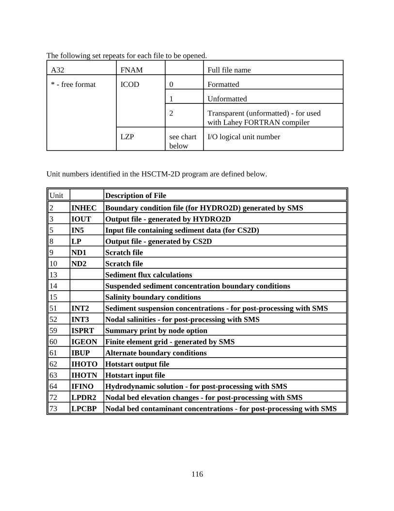
The following set repeats for each file to be opened.
A32 FNAM Full file name
* - free format ICOD 0 Formatted
1 Unformatted
2 Transparent (unformatted) - for used with Lahey FORTRAN compiler
LZP see chart I/O logical unit number below
Unit numbers identified in the HSCTM-2D program are defined below.
Unit Description of File
2 INHEC Boundary condition file (for HYDRO2D) generated by SMS 3 IOUT Output file - generated by HYDRO2D 5 IN5 Input file containing sediment data (for CS2D) 8 LP Output file - generated by CS2D 9 ND1 Scratch file 10 ND2 Scratch file 13 Sediment flux calculations 14 Suspended sediment concentration boundary conditions 15 Salinity boundary conditions 51 INT2 Sediment suspension concentrations - for post-processing with SMS 52 INT3 Nodal salinities - for post-processing with SMS 59 ISPRT Summary print by node option 60 IGEON Finite element grid - generated by SMS 61 IBUP Alternate boundary conditions 62 IHOTO Hotstart output file 63 IHOTN Hotstart input file 64 IFINO Hydrodynamic solution - for post-processing with SMS 72 LPDR2 Nodal bed elevation changes - for post-processing with SMS 73 LPCBP Nodal bed contaminant concentrations - for post-processing with SMS
116
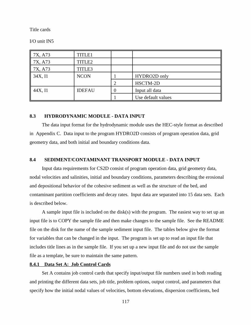
Title cards
I/O unit IN5
7X, A73 TITLE1
7X, A73 TITLE2
7X, A73 TITLE3
34X, I1 NCON 1 HYDRO2D only
2 HSCTM-2D
44X, I1 IDEFAU 0 Input all data
1 Use default values
8.3 HYDRODYNAMIC MODULE - DATA INPUT
The data input format for the hydrodynamic module uses the HEC-style format as described
in Appendix C. Data input to the program HYDRO2D consists of program operation data, grid
geometry data, and both initial and boundary conditions data.
8.4 SEDIMENT/CONTAMINANT TRANSPORT MODULE - DATA INPUT
Input data requirements for CS2D consist of program operation data, grid geometry data,
nodal velocities and salinities, initial and boundary conditions, parameters describing the erosional
and depositional behavior of the cohesive sediment as well as the structure of the bed, and
contaminant partition coefficients and decay rates. Input data are separated into 15 data sets. Each
is described below.
A sample input file is included on the disk(s) with the program. The easiest way to set up an
input file is to COPY the sample file and then make changes to the sample file. See the README
file on the disk for the name of the sample sediment input file. The tables below give the format
for variables that can be changed in the input. The program is set up to read an input file that
includes title lines as in the sample file. If you set up a new input file and do not use the sample
file as a template, be sure to maintain the same pattern.
8.4.1 Data Set A: Job Control Cards
Set A contains job control cards that specify input/output file numbers used in both reading
and printing the different data sets, job title, problem options, output control, and parameters that
specify how the initial nodal values of velocities, bottom elevations, dispersion coefficients, bed
117
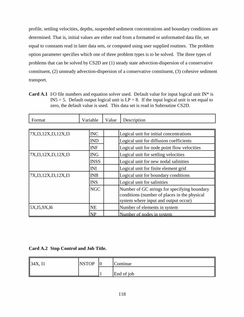
profile, settling velocities, depths, suspended sediment concentrations and boundary conditions are
determined. That is, initial values are either read from a formatted or unformatted data file, set
equal to constants read in later data sets, or computed using user supplied routines. The problem
option parameter specifies which one of three problem types is to be solved. The three types of
problems that can be solved by CS2D are (1) steady state advection-dispersion of a conservative
constituent, (2) unsteady advection-dispersion of a conservative constituent, (3) cohesive sediment
transport.
Card A.1 I/O file numbers and equation solver used. Default value for input logical unit IN* is IN5 = 5. Default output logical unit is LP = 8. If the input logical unit is set equal to zero, the default value is used. This data set is read in Subroutine CS2D.
Format Variable Value Description
7X,I3,12X,I3,12X,I3 INC Logical unit for initial concentrations
IND Logical unit for diffusion coefficients
INF Logical unit for node point flow velocities
7X,I3,12X,I3,12X,I3 ING Logical unit for settling velocities
INSS Logical unit for new nodal salinities
INI Logical unit for finite element grid
7X,I3,12X,I3,12X,I3 INB Logical unit for boundary conditions
INS Logical unit for salinities
NGC Number of GC strings for specifying boundary conditions (number of places in the physical system where input and output occur)
5X,I5,9X,I6 NE Number of elements in system
NP Number of nodes in system
Card A.2 Stop Control and Job Title.
34X, I1 NSTOP 0 Continue
1 End of job
118
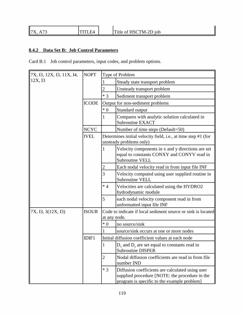
7X, A73 TITLE4 Title of HSCTM-2D job
8.4.2 Data Set B: Job Control Parameters
Card B.1 Job control parameters, input codes, and problem options.
7X, I3, 12X, I3, 11X, I4, NOPT Type of Problem 12X, I3 1 Steady state transport problem
2 Unsteady transport problem
* 3 Sediment transport problem
ICODE Output for non-sediment problems
* 0 Standard output
1 Compares with analytic solution calculated in Subroutine EXACT
NCYC Number of time steps (Default=50)
IVEL Determines initial velocity field, i.e., at time step #1 (for unsteady problems only)
1 Velocity components in x and y directions are set equal to constants CONXY and CONYV read in Subroutine VELL
2 Each nodal velocity read in from input file INF
3 Velocity computed using user supplied routine in Subroutine VELL
* 4 Velocities are calculated using the HYDRO2 hydrodynamic module
5 each nodal velocity component read in from unformatted input file INF
7X, I3, 3(12X, I3) ISOUR Code to indicate if local sediment source or sink is located at any node.
* 0 no source/sink
1 source/sink occurs at one or more nodes
IDIF1 Initial diffusion coefficient values at each node
1 Dx and Dy are set equal to constants read in Subroutine DISPER
2 Nodal diffusion coefficients are read in from file number IND
* 3 Diffusion coefficients are calculated using user supplied procedure [NOTE: the procedure in the program is specific to the example problem]
119

IBED Initial bed profile
0 No sediment present on bed
* 1 Bed profile read in Subroutine ORGBED
ISET Initial settling velocity at each node.
1 Set to a constant read in Subroutine SETVEL.
2 Each nodal settling velocity is read in from formatted file number ING.
* 3 Settling velocities are computed using settling velocity model in Subroutine SETVEL
7X, I3, 3(12X, I3) ICONC Initial suspended sediment concentrations.
* 1 Set to constant
2 Read in from file number INC
3 Computed according to user supplied procedure in subroutine CONCIC
INBC Boundary conditions
* 1 Each value read in from formatted file number INB
2 Computed in Subroutine CONCBC using user supplied routine
3 Each value read in from unformatted file number INB. Boundary node array MFIX and Boundary condition array SPEC are both read in.
IDRY Code to indicate dry node (i.e., negative flow depth) problem.
* 0 No dry nodes will occur
1 Possible dry nodes
ISZ Temporal flow classification
* 0 Unsteady flow
1 Steady state flow
120

8.4.3 Data Set C: Transient Problem Input
Transient control parameters are specified in Set C. Input data include time step size, degree
of implicitness for the Crank-Nicolson type time-marching scheme used in CS2D, and transient
code arrays that specify at which time steps during a dynamic simulation new values of one or
more of the parameters listed under Data Set B are read in or calculated. One of the code arrays
also specifies the type of output (e.g., nodal concentrations and/or discretized bed profiles), if any,
desired at each time step.
Card C.1 Transient input
30X, F10.4 TETA Degree of implicitness for Crank-Nicolson time marching scheme. (Default = 0.6667)
0 explicit
1 implicit
16X, F9.1 DELT Time step - [hour] (should be of the order 0.083 -0.5 hr for sediment transport problems in estuaries)
16X, F9.2 TIM(1) Start time - [hr]. (Default = 0.0)
I4 IOSTEP Frequency of full output
I4 NSTIME Time step number at which to start program
Card C.2 Information for FLUX Routine
I1, I10 IFLX Flux routine switch
0 sedflux off
1 sedflux on
IFLXNP Number of nodes in the FLUX string
5I10 IFLXNN Node numbers of nodes in the flux string. If using SMS, the node numbers can be identified with that program. If there are less than 17 node nos., you need to know how the compiler handles this READ statement; e.g., when there are
5I10 IFLXNN
5I10 IFLXNN 5 nodes, the SALFORD compiler requires 1 line of input and 1 blank line.2I10 IFLXNN
121
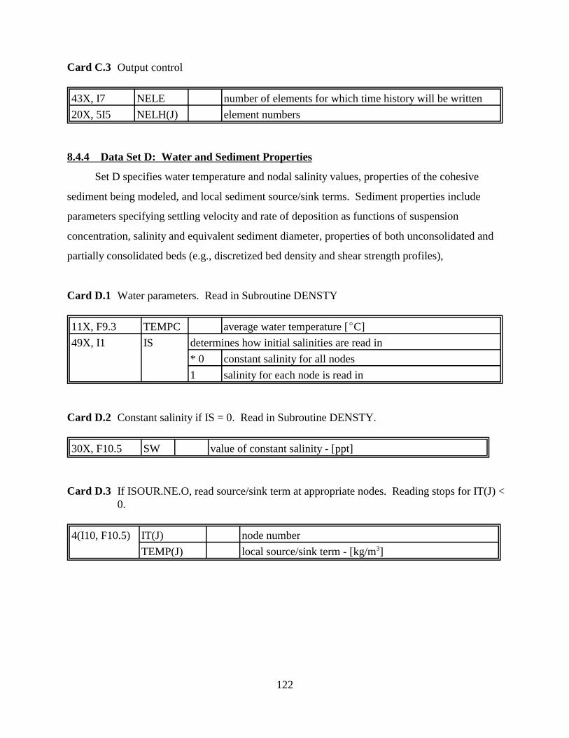
Card C.3 Output control
43X, I7 NELE number of elements for which time history will be written
20X, 5I5 NELH(J) element numbers
8.4.4 Data Set D: Water and Sediment Properties
Set D specifies water temperature and nodal salinity values, properties of the cohesive
sediment being modeled, and local sediment source/sink terms. Sediment properties include
parameters specifying settling velocity and rate of deposition as functions of suspension
concentration, salinity and equivalent sediment diameter, properties of both unconsolidated and
partially consolidated beds (e.g., discretized bed density and shear strength profiles),
Card D.1 Water parameters. Read in Subroutine DENSTY
11X, F9.3 TEMPC average water temperature [EC]
49X, I1 IS determines how initial salinities are read in
* 0 constant salinity for all nodes
1 salinity for each node is read in
Card D.2 Constant salinity if IS = 0. Read in Subroutine DENSTY.
30X, F10.5 SW value of constant salinity - [ppt]
Card D.3 If ISOUR.NE.O, read source/sink term at appropriate nodes. Reading stops for IT(J) < 0.
4(I10, F10.5) IT(J) node number
TEMP(J) local source/sink term - [kg/m3]
122
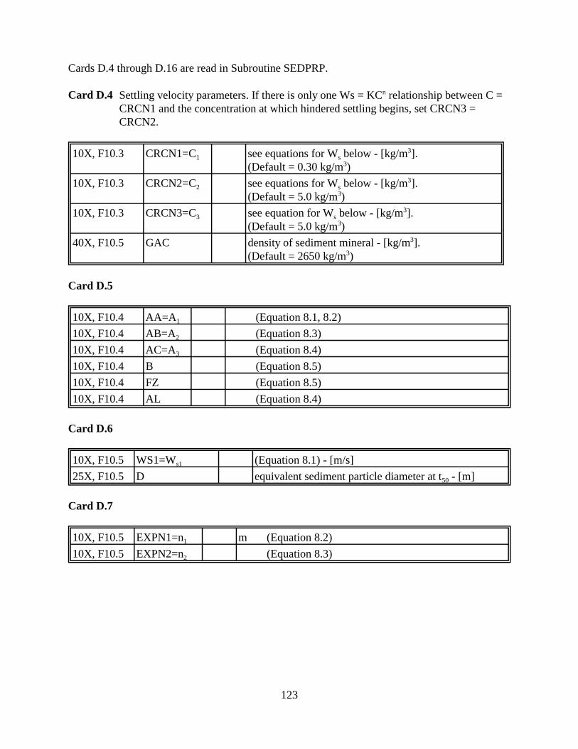
Cards D.4 through D.16 are read in Subroutine SEDPRP.
Card D.4 Settling velocity parameters. If there is only one Ws = KCn relationship between C = CRCN1 and the concentration at which hindered settling begins, set CRCN3 = CRCN2.
10X, F10.3 CRCN1=C1 see equations for Ws below - [kg/m3]. (Default = 0.30 kg/m3)
10X, F10.3 CRCN2=C2 see equations for Ws below - [kg/m3]. (Default = 5.0 kg/m3)
10X, F10.3 CRCN3=C3 see equation for Ws below - [kg/m3]. (Default = 5.0 kg/m3)
40X, F10.5 GAC density of sediment mineral - [kg/m3]. (Default = 2650 kg/m3)
Card D.5
10X, F10.4 AA=A1 (Equation 8.1, 8.2)
10X, F10.4 AB=A2 (Equation 8.3)
10X, F10.4 AC=A3 (Equation 8.4)
10X, F10.4 B (Equation 8.5)
10X, F10.4 FZ (Equation 8.5)
10X, F10.4 AL (Equation 8.4)
Card D.6
10X, F10.5 WS1=Ws1 (Equation 8.1) - [m/s]
25X, F10.5 D equivalent sediment particle diameter at t50 - [m]
Card D.7
10X, F10.5 EXPN1=n1 m (Equation 8.2)
10X, F10.5 EXPN2=n2 (Equation 8.3)
123
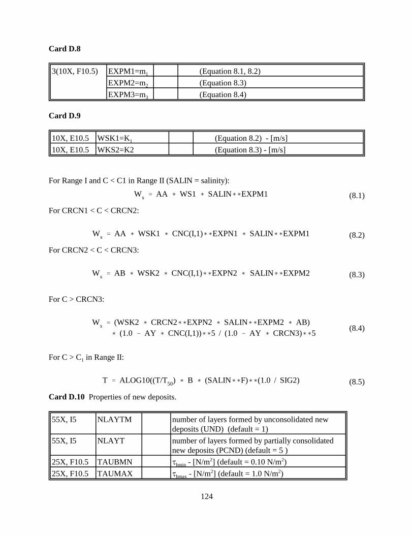
Card D.8
3(10X, F10.5) EXPM1=m1 (Equation 8.1, 8.2)
EXPM2=m2 (Equation 8.3)
EXPM3=m3 (Equation 8.4)
Card D.9
10X, E10.5 WSK1=K1 (Equation 8.2) - [m/s]
10X, E10.5 WKS2=K2 (Equation 8.3) - [m/s]
For Range I and C < C1 in Range II (SALIN = salinity):
W ' AA ( WS1 ( SALIN((EXPM1 (8.1)s
For CRCN1 < C < CRCN2:
W ' AA ( WSK1 ( CNC(I,1)((EXPN1 ( SALIN((EXPM1 (8.2)s
For CRCN2 < C < CRCN3:
W ' AB ( WSK2 ( CNC(I,1)((EXPN2 ( SALIN((EXPM2 (8.3)s
For C > CRCN3:
W ' (WSK2 ( CRCN2((EXPN2 ( SALIN((EXPM2 ( AB)s (8.4)( (1.0 & AY ( CNC(I,1))((5 / (1.0 & AY ( CRCN3)((5
For C > C1 in Range II:
T ' ALOG10((T/T50) ( B ( (SALIN((F)(((1.0 / SIG2) (8.5)
Card D.10 Properties of new deposits.
55X, I5 NLAYTM number of layers formed by unconsolidated new deposits (UND) (default = 1)
55X, I5 NLAYT number of layers formed by partially consolidated new deposits (PCND) (default = 5 )
25X, F10.5 TAUBMN Jbmin - [N/m2] (default = 0.10 N/m2)
25X, F10.5 TAUMAX Jbmax - [N/m2] (default = 1.0 N/m2)
124
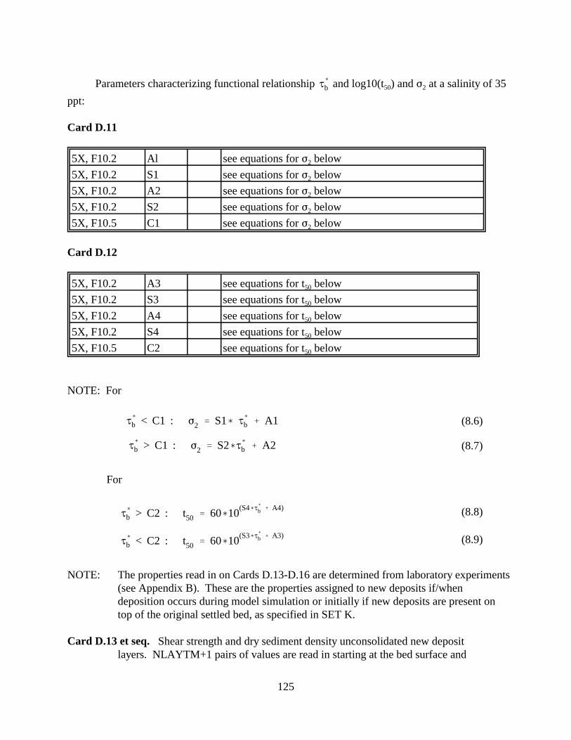
Parameters characterizing functional relationship J( and log10(t50) and F2 at a salinity of 35 b
ppt:
Card D.11
5X, F10.2 Al see equations for F2 below
5X, F10.2 S1 see equations for F2 below
5X, F10.2 A2 see equations for F2 below
5X, F10.2 S2 see equations for F2 below
5X, F10.5 C1 see equations for F2 below
Card D.12
5X, F10.2 A3 see equations for t50 below
5X, F10.2 S3 see equations for t50 below
5X, F10.2 A4 see equations for t50 below
5X, F10.2 S4 see equations for t50 below
5X, F10.5 C2 see equations for t50 below
NOTE: For
J( b < C1 : F2 ' S1( J(
b % A1 (8.6)
J( b > C1 : F2 ' S2(J(
b % A2 (8.7)
For
J( b > C2 : t50 ' 60(10
(S4(J( b % A4) (8.8)
J( b < C2 : t50 ' 60(10
(S3(J( b % A3) (8.9)
NOTE: The properties read in on Cards D.13-D.16 are determined from laboratory experiments (see Appendix B). These are the properties assigned to new deposits if/when deposition occurs during model simulation or initially if new deposits are present on top of the original settled bed, as specified in SET K.
Card D.13 et seq. Shear strength and dry sediment density unconsolidated new deposit layers. NLAYTM+1 pairs of values are read in starting at the bed surface and
125
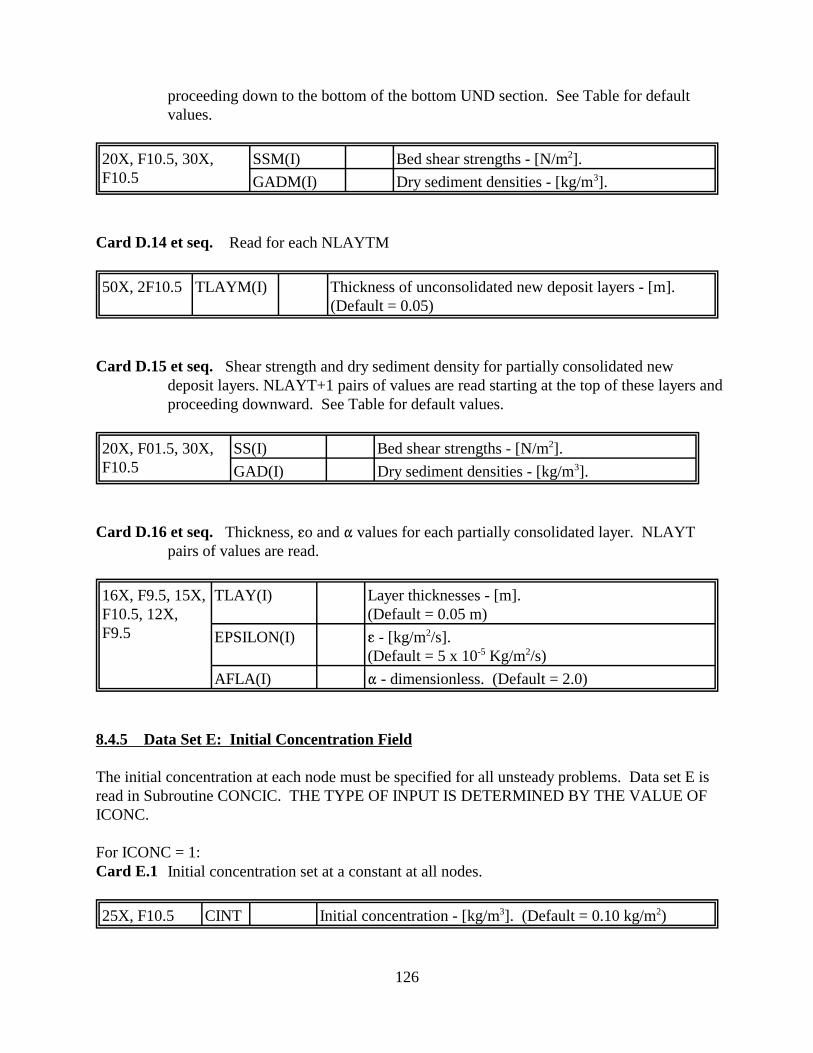
proceeding down to the bottom of the bottom UND section. See Table for default values.
20X, F10.5, 30X, SSM(I) Bed shear strengths - [N/m2]. F10.5 GADM(I) Dry sediment densities - [kg/m3].
Card D.14 et seq. Read for each NLAYTM
50X, 2F10.5 TLAYM(I) Thickness of unconsolidated new deposit layers - [m]. (Default = 0.05)
Card D.15 et seq. Shear strength and dry sediment density for partially consolidated new deposit layers. NLAYT+1 pairs of values are read starting at the top of these layers and proceeding downward. See Table for default values.
20X, F01.5, 30X, SS(I) Bed shear strengths - [N/m2]. F10.5 GAD(I) Dry sediment densities - [kg/m3].
Card D.16 et seq. Thickness, go and " values for each partially consolidated layer. NLAYT pairs of values are read.
16X, F9.5, 15X, TLAY(I) Layer thicknesses - [m]. F10.5, 12X, (Default = 0.05 m) F9.5 EPSILON(I) g - [kg/m2/s].
(Default = 5 x 10⁻⁵ Kg/m2/s)
AFLA(I) " - dimensionless. (Default = 2.0)
8.4.5 Data Set E: Initial Concentration Field
The initial concentration at each node must be specified for all unsteady problems. Data set E isread in Subroutine CONCIC. THE TYPE OF INPUT IS DETERMINED BY THE VALUE OFICONC.
For ICONC = 1:Card E.1 Initial concentration set at a constant at all nodes.
25X, F10.5 CINT Initial concentration - [kg/m3]. (Default = 0.10 kg/m2)
126
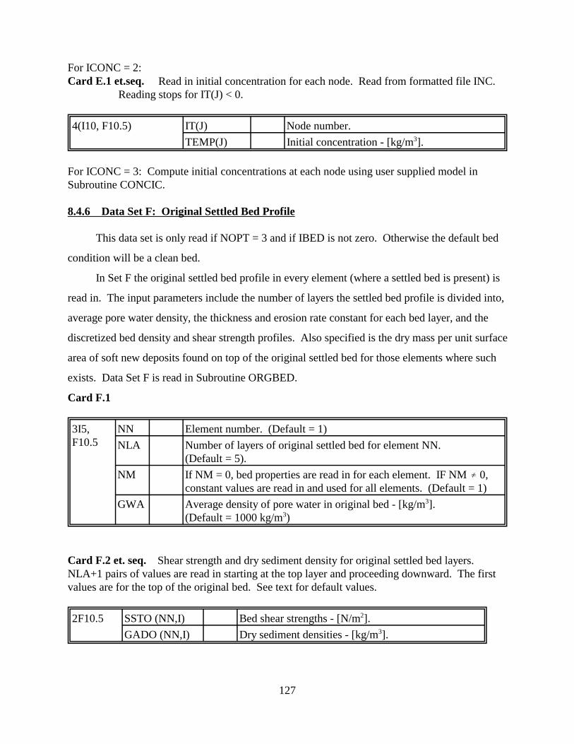
For ICONC = 2: Card E.1 et.seq. Read in initial concentration for each node. Read from formatted file INC.
Reading stops for IT(J) < 0.
4(I10, F10.5) IT(J) Node number.
TEMP(J) Initial concentration - [kg/m3].
For ICONC = 3: Compute initial concentrations at each node using user supplied model in Subroutine CONCIC.
8.4.6 Data Set F: Original Settled Bed Profile
This data set is only read if NOPT = 3 and if IBED is not zero. Otherwise the default bed
condition will be a clean bed.
In Set F the original settled bed profile in every element (where a settled bed is present) is
read in. The input parameters include the number of layers the settled bed profile is divided into,
average pore water density, the thickness and erosion rate constant for each bed layer, and the
discretized bed density and shear strength profiles. Also specified is the dry mass per unit surface
area of soft new deposits found on top of the original settled bed for those elements where such
exists. Data Set F is read in Subroutine ORGBED.
Card F.1
3I5, NN Element number. (Default = 1) F10.5 NLA Number of layers of original settled bed for element NN.
(Default = 5).
NM If NM = 0, bed properties are read in for each element. IF NM Ö 0, constant values are read in and used for all elements. (Default = 1)
GWA Average density of pore water in original bed - [kg/m3]. (Default = 1000 kg/m3)
Card F.2 et. seq. Shear strength and dry sediment density for original settled bed layers. NLA+1 pairs of values are read in starting at the top layer and proceeding downward. The first values are for the top of the original bed. See text for default values.
2F10.5 SSTO (NN,I) Bed shear strengths - [N/m2].
GADO (NN,I) Dry sediment densities - [kg/m3].
127
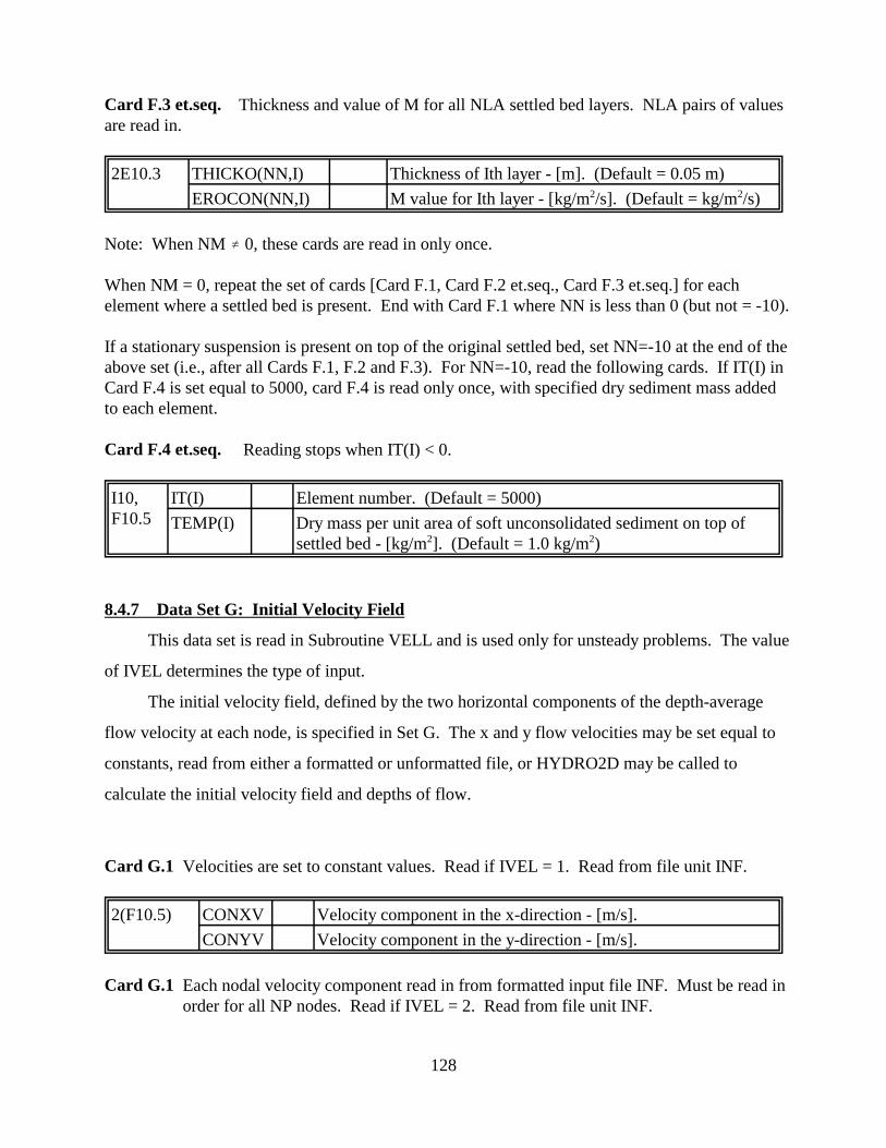
Card F.3 et.seq. Thickness and value of M for all NLA settled bed layers. NLA pairs of values are read in.
2E10.3 THICKO(NN,I) Thickness of Ith layer - [m]. (Default = 0.05 m)
EROCON(NN,I) M value for Ith layer - [kg/m2/s]. (Default = kg/m2/s)
Note: When NM Ö 0, these cards are read in only once.
When NM = 0, repeat the set of cards [Card F.1, Card F.2 et.seq., Card F.3 et.seq.] for each element where a settled bed is present. End with Card F.1 where NN is less than 0 (but not = -10).
If a stationary suspension is present on top of the original settled bed, set NN=-10 at the end of the above set (i.e., after all Cards F.1, F.2 and F.3). For NN=-10, read the following cards. If IT(I) in Card F.4 is set equal to 5000, card F.4 is read only once, with specified dry sediment mass added to each element.
Card F.4 et.seq. Reading stops when IT(I) < 0.
I10, IT(I) Element number. (Default = 5000) F10.5 TEMP(I) Dry mass per unit area of soft unconsolidated sediment on top of
settled bed - [kg/m2]. (Default = 1.0 kg/m2)
8.4.7 Data Set G: Initial Velocity Field
This data set is read in Subroutine VELL and is used only for unsteady problems. The value
of IVEL determines the type of input.
The initial velocity field, defined by the two horizontal components of the depth-average
flow velocity at each node, is specified in Set G. The x and y flow velocities may be set equal to
constants, read from either a formatted or unformatted file, or HYDRO2D may be called to
calculate the initial velocity field and depths of flow.
Card G.1 Velocities are set to constant values. Read if IVEL = 1. Read from file unit INF.
2(F10.5) CONXV Velocity component in the x-direction - [m/s].
CONYV Velocity component in the y-direction - [m/s].
Card G.1 Each nodal velocity component read in from formatted input file INF. Must be read in order for all NP nodes. Read if IVEL = 2. Read from file unit INF.
128
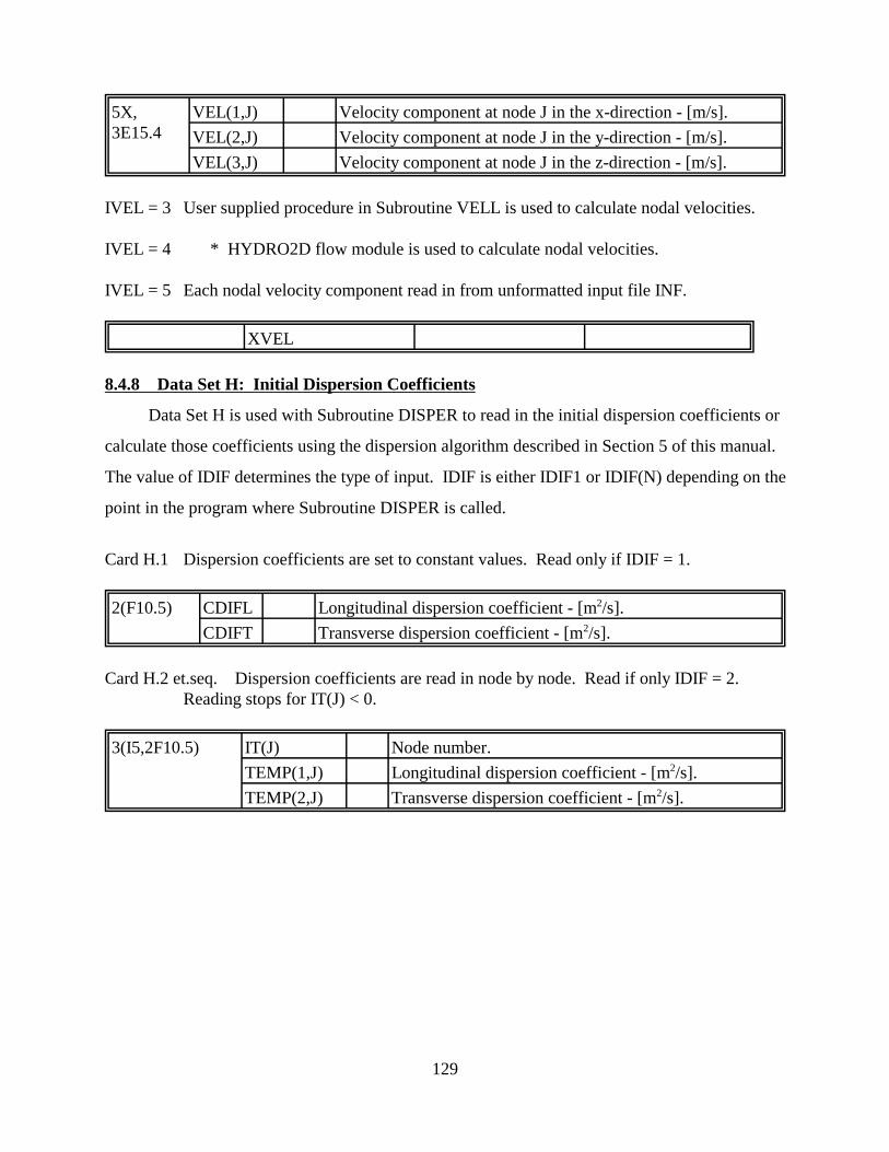
5X, VEL(1,J) Velocity component at node J in the x-direction - [m/s]. 3E15.4 VEL(2,J) Velocity component at node J in the y-direction - [m/s].
VEL(3,J) Velocity component at node J in the z-direction - [m/s].
IVEL = 3 User supplied procedure in Subroutine VELL is used to calculate nodal velocities.
IVEL = 4 * HYDRO2D flow module is used to calculate nodal velocities.
IVEL = 5 Each nodal velocity component read in from unformatted input file INF.
XVEL
8.4.8 Data Set H: Initial Dispersion Coefficients
Data Set H is used with Subroutine DISPER to read in the initial dispersion coefficients or
calculate those coefficients using the dispersion algorithm described in Section 5 of this manual.
The value of IDIF determines the type of input. IDIF is either IDIF1 or IDIF(N) depending on the
point in the program where Subroutine DISPER is called.
Card H.1 Dispersion coefficients are set to constant values. Read only if IDIF = 1.
2(F10.5) CDIFL Longitudinal dispersion coefficient - [m2/s].
CDIFT Transverse dispersion coefficient - [m2/s].
Card H.2 et.seq. Dispersion coefficients are read in node by node. Read if only IDIF = 2. Reading stops for IT(J) < 0.
3(I5,2F10.5) IT(J) Node number.
TEMP(1,J) Longitudinal dispersion coefficient - [m2/s].
TEMP(2,J) Transverse dispersion coefficient - [m2/s].
129
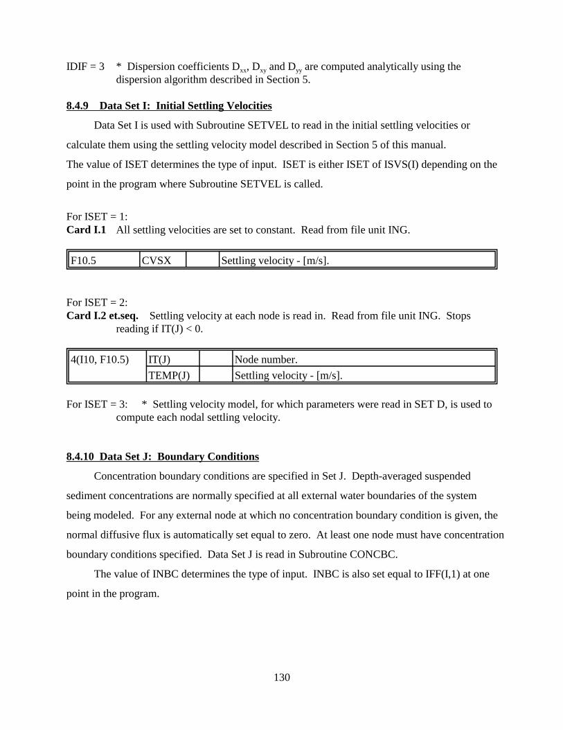
IDIF = 3 * Dispersion coefficients Dxx, Dxy and Dyy are computed analytically using the dispersion algorithm described in Section 5.
8.4.9 Data Set I: Initial Settling Velocities
Data Set I is used with Subroutine SETVEL to read in the initial settling velocities or
calculate them using the settling velocity model described in Section 5 of this manual.
The value of ISET determines the type of input. ISET is either ISET of ISVS(I) depending on the
point in the program where Subroutine SETVEL is called.
For ISET = 1:Card I.1 All settling velocities are set to constant. Read from file unit ING.
F10.5 CVSX Settling velocity - [m/s].
For ISET = 2: Card I.2 et.seq. Settling velocity at each node is read in. Read from file unit ING. Stops
reading if IT(J) < 0.
4(I10, F10.5) IT(J) Node number.
TEMP(J) Settling velocity - [m/s].
For ISET = 3: * Settling velocity model, for which parameters were read in SET D, is used to compute each nodal settling velocity.
8.4.10 Data Set J: Boundary Conditions
Concentration boundary conditions are specified in Set J. Depth-averaged suspended
sediment concentrations are normally specified at all external water boundaries of the system
being modeled. For any external node at which no concentration boundary condition is given, the
normal diffusive flux is automatically set equal to zero. At least one node must have concentration
boundary conditions specified. Data Set J is read in Subroutine CONCBC.
The value of INBC determines the type of input. INBC is also set equal to IFF(I,1) at one
point in the program.
130

For INBC = 1:Card J.1 et.seq. Node number and specified boundary condition. Read from file unit INB.
3(I10, F10.5) IT(J) Node number
TEMP(J) Specified concentration - [kg/m3].
For INBC = 2: * Concentration computed according to user supplied procedure in Subroutine CONCBC.
For INBC = 3: Card J.2 et.seq. Specified boundary conditions. Must be read in order for all NP nodes.
Read from unformatted file INB.
MFIX(J) Equal to 1 for boundary node; 0 for all other nodes.
SPEC(J,1) Specified concentration at node J - [kg/m3].
8.4.11 Data Set K: New Salinities
In Set K nodal salinity values are read in from either a formatted or unformatted file, or a
constant salinity may be assigned to all nodes. The type of input is determined by the value of
ISALC(J), for J=2,....,NTTS. The logical unit for the input is INSS.
For ISALC(J) = 1:Card K.1 Assign constant salinity value to each node.
30X, F10.5 SW Constant salinity value - [ppt].
For ISALC(J) = 2:Card K.2 New salinities for all nodes. Reading stops when IT(J) < 0.
3(I10, F10.5) IT(J) Node number.
TEMP(J) Salinity at jth node.
8.4.12 Data Set L: Dynamic Input
Dynamic input is specified in Set L that contains the required data to update the following
parameters at the time steps specified in Set C: salinities, concentration boundary conditions,
depths of flow, velocities, dispersion coefficients and settling velocities. If the code array value
for a particular parameter at a given time step is zero, no input is required. If parameter update is
required, the current value of the code array will determine the type of input.
131

The same subroutines that read initial values are used to read changes in these values during
a dynamic run. The input code arrays in SET C tell the program if any new values should be read
in at each time step. Note that the starting time is time step 1. The order of reading each set of
data is given below.
DESCRIPTION CODE ARRAY INPUT CARD SET
SUBROUTINE
Salinities ISALC(J) SET K
Concentration B.C. IFF(J,1) SET J CONCBC
Velocities IVOD(J) SET F CS2D
Dispersion Coefficients IDIF(J) SET E CONCIC
Settling Velocities ISVS(J) SET J DISPER
8.5 DATA MANAGEMENT
The large amount of data required to operate the CS2D modeling system in either the default
or non-default mode necessitates careful preparation of the input data sets. The information
contained in this section should be closely followed during the process. The flow chart of the
main components of HSCTM-2D (in Appendix A) should be referred to in particular to assist the
user in structuring the data sets for the various program options, whereas the flow charts and data
input instructions for HYDRO2D and CS2D should be used to enter the correct data in the
specified order and format. The data sets for the example problem described in Section 9 provide
examples of proper data set organization. There exists (at present) no built-in or programmed
assistance for inputting the required data at. The development of routines to make this operation
"user friendly" is planned for future versions of the modeling system.
8.6 DEFAULT OPTION
The parameters for which default values are used when the default option is invoked
(IDEFAU = 1) are indicated by asterisks in the listing in this chapter. Values of the default
parameters are listed in Table 8.1. It is once again emphasized that the results obtained using the
default option should be considered indicative of qualitative trends only, and used only for relative
comparisons among different sites and/or designs.
132
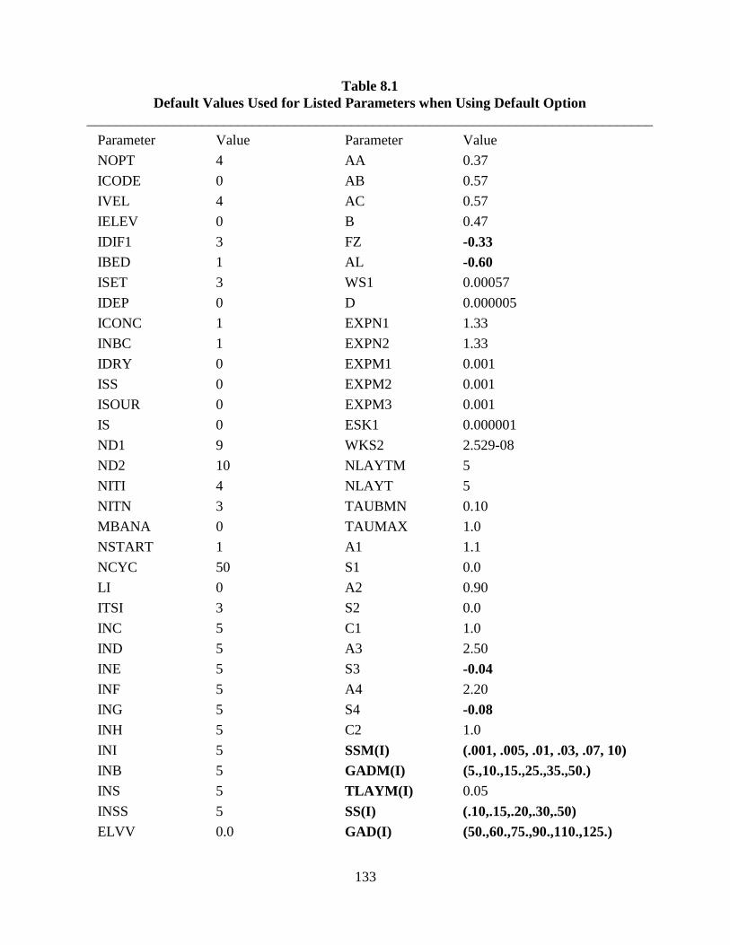
_______________________________________________________________________________
Table 8.1 Default Values Used for Listed Parameters when Using Default Option
Parameter Value Parameter Value
NOPT 4 AA 0.37
ICODE 0 AB 0.57
IVEL 4 AC 0.57
IELEV 0 B 0.47
IDIF1 3 FZ -0.33 IBED 1 AL -0.60 ISET 3 WS1 0.00057
IDEP 0 D 0.000005
ICONC 1 EXPN1 1.33
INBC 1 EXPN2 1.33
IDRY 0 EXPM1 0.001
ISS 0 EXPM2 0.001
ISOUR 0 EXPM3 0.001
IS 0 ESK1 0.000001
ND1 9 WKS2 2.529-08
ND2 10 NLAYTM 5
NITI 4 NLAYT 5
NITN 3 TAUBMN 0.10
MBANA 0 TAUMAX 1.0
NSTART 1 A1 1.1
NCYC 50 S1 0.0
LI 0 A2 0.90
ITSI 3 S2 0.0
INC 5 C1 1.0
IND 5 A3 2.50
INE 5 S3 -0.04 INF 5 A4 2.20
ING 5 S4 -0.08 INH 5 C2 1.0
INI 5 SSM(I) (.001, .005, .01, .03, .07, 10) INB 5 GADM(I) (5.,10.,15.,25.,35.,50.) INS 5 TLAYM(I) 0.05
INSS 5 SS(I) (.10,.15,.20,.30,.50) ELVV 0.0 GAD(I) (50.,60.,75.,90.,110.,125.)
133

Parameter Value Parameter Value
XSCALE 1.0 TLAY(I) 0.05
YSCALE 1.0 EPSLON(I) 5.0E-05 DSET 0.0 AFLA(I) 5.0
DSETD 0.0 ORT(I) 50000.
TETA 0.6667 CRCN3 5.0
CRCN1 0.30 GAC 2650.0
134
SECTION 9
EXAMPLE PROBLEM
The utility of the HSCTM-2D modeling system is demonstrated by simulating the tidal flow and
sediment transport in Winyah Bay, South Carolina. The portion of Winyah Bay modeled is shown
in Figure 9.1. It must be emphasized that only a limited field study was conducted at this site, and
therefore the results presented herein should be considered as demonstrative in nature only. A second
example problem that demonstrates the contaminant transport capabilities of HSCTM-2D will be
included in the second edition of this user manual.
Data used in modeling the flow and cohesive sediment transport, some of which were obtained
during a limited two-day field study, included estuary geometry and bathymetry from NOAA
navigation maps for Winyah Bay, and bathymetry of the Belle Isle marina from a post-dredge survey.
Tides at the boundaries of the model grid were obtained using the TIDE1 Rise & Fall (TM) Software.
The predicted tides were used for boundary conditions in the hydrodynamic module. A median
sediment diameter of 50 µm, settling velocity of 10-5 m/s, and an average initial background
suspension concentration of 10 mg/l were used. Spatially nonuniform, sinusoidally varying suspended
sediment concentrations were used for the upstream and downstream open water boundary conditions
for the sediment transport module. The slack tide (minima) concentrations at both boundaries were
taken to be 10 mg/l, while maximum flood concentrations of 65 mg/l and 45 mg/l occurred at the
upstream and downstream boundaries, respectively, and maximum ebb concentrations of 60 mg/l and
40 mg/l occurred at the upstream and downstream boundaries, respectively. These concentrations
were representative of the suspension concentrations determined from water samples collected over
two tidal cycles during the two-day field study. The finite element grid used to represent the portion
135
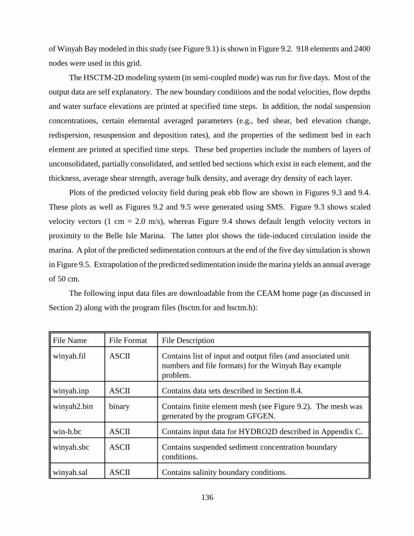
of Winyah Bay modeled in this study (see Figure 9.1) is shown in Figure 9.2. 918 elements and 2400
nodes were used in this grid.
The HSCTM-2D modeling system (in semi-coupled mode) was run for five days. Most of the
output data are self explanatory. The new boundary conditions and the nodal velocities, flow depths
and water surface elevations are printed at specified time steps. In addition, the nodal suspension
concentrations, certain elemental averaged parameters (e.g., bed shear, bed elevation change,
redispersion, resuspension and deposition rates), and the properties of the sediment bed in each
element are printed at specified time steps. These bed properties include the numbers of layers of
unconsolidated, partially consolidated, and settled bed sections which exist in each element, and the
thickness, average shear strength, average bulk density, and average dry density of each layer.
Plots of the predicted velocity field during peak ebb flow are shown in Figures 9.3 and 9.4.
These plots as well as Figures 9.2 and 9.5 were generated using SMS. Figure 9.3 shows scaled
velocity vectors (1 cm = 2.0 m/s), whereas Figure 9.4 shows default length velocity vectors in
proximity to the Belle Isle Marina. The latter plot shows the tide-induced circulation inside the
marina. A plot of the predicted sedimentation contours at the end of the five day simulation is shown
in Figure 9.5. Extrapolation of the predicted sedimentation inside the marina yields an annual average
of 50 cm.
The following input data files are downloadable from the CEAM home page (as discussed in
Section 2) along with the program files (hsctm.for and hsctm.h):
File Name File Format File Description
winyah.fil ASCII Contains list of input and output files (and associated unit numbers and file formats) for the Winyah Bay example problem.
winyah.inp ASCII Contains data sets described in Section 8.4.
winyah2.bin binary Contains finite element mesh (see Figure 9.2). The mesh was generated by the program GFGEN.
win-h.bc ASCII Contains input data for HYDRO2D described in Appendix C.
winyah.sbc ASCII Contains suspended sediment concentration boundary conditions.
winyah.sal ASCII Contains salinity boundary conditions.
136
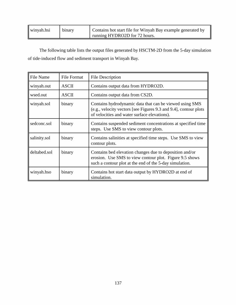
winyah.hsi binary Contains hot start file for Winyah Bay example generated by running HYDRO2D for 72 hours.
The following table lists the output files generated by HSCTM-2D from the 5-day simulation
of tide-induced flow and sediment transport in Winyah Bay.
File Name File Format File Description
winyah.out ASCII Contains output data from HYDRO2D.
wsed.out ASCII Contains output data from CS2D.
winyah.sol binary Contains hydrodynamic data that can be viewed using SMS (e.g., velocity vectors [see Figures 9.3 and 9.4], contour plots of velocities and water surface elevations).
sedconc.sol binary Contains suspended sediment concentrations at specified time steps. Use SMS to view contour plots.
salinity.sol binary Contains salinities at specified time steps. Use SMS to view contour plots.
deltabed.sol binary Contains bed elevation changes due to deposition and/or erosion. Use SMS to view contour plot. Figure 9.5 shows such a contour plot at the end of the 5-day simulation.
winyah.hso binary Contains hot start data output by HYDRO2D at end of simulation.
137
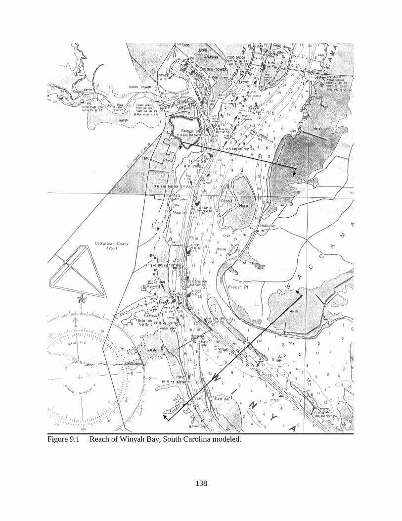
Figure 9.1 Reach of Winyah Bay, South Carolina modeled.
138
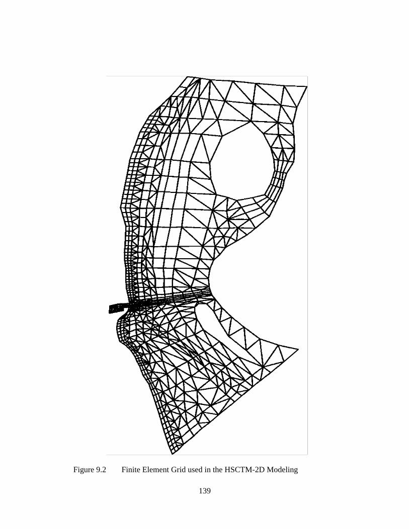
Figure 9.2 Finite Element Grid used in the HSCTM-2D Modeling
139
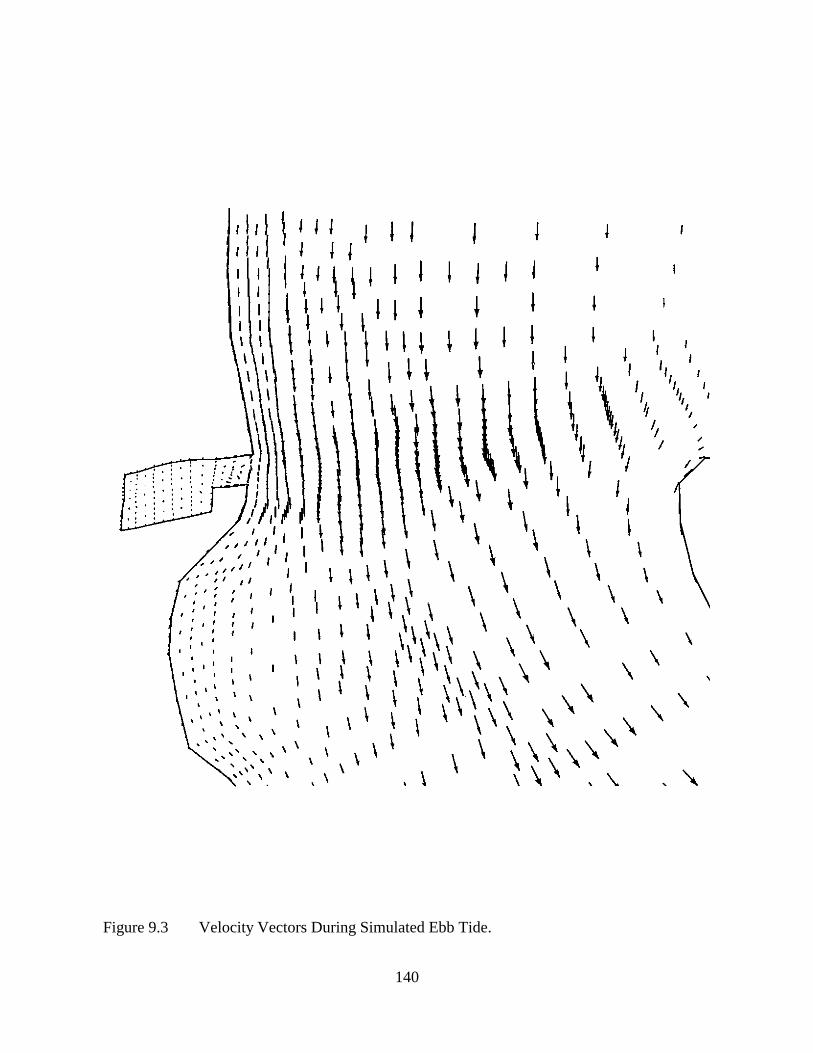
Figure 9.3 Velocity Vectors During Simulated Ebb Tide.
140
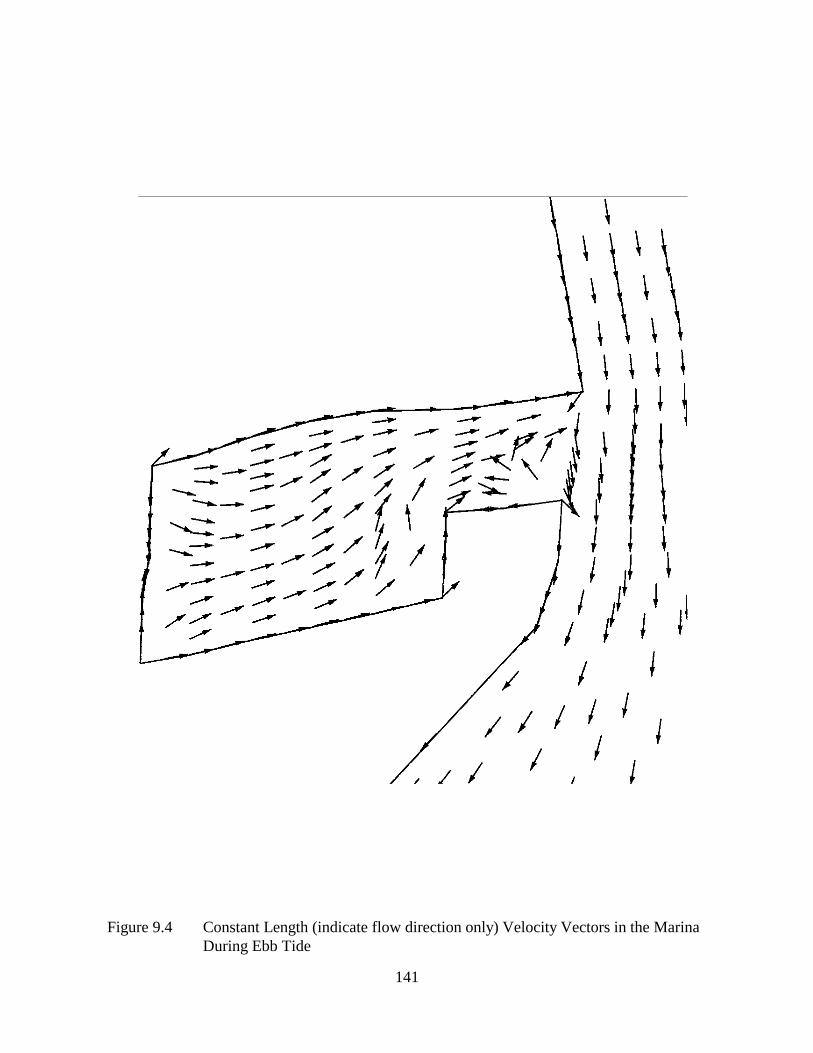
Figure 9.4 Constant Length (indicate flow direction only) Velocity Vectors in the Marina During Ebb Tide
141
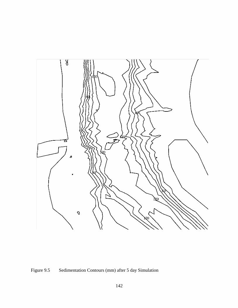
Figure 9.5 Sedimentation Contours (mm) after 5 day Simulation
142
REFERENCES
Allersma, E., "Mud in Estuaries and Along Coasts," International Symposium on River Sedimentation, Beijing, P. R. of China, March, 1980.
Allison, L.E., Organic Carbon, Part II, American Society of Agronomy, Madison, Wisconsin, 1965.
Ariathurai, R., A Finite Element Model for Sediment Transport in Estuaries, Ph.d. Dissertation, University of California, Davis, California, 1974.
Ariathurai, R., and R.B. Krone, "Finite Element Model for Cohesive Sediment Transport," Journal of the Hydraulics Division, ASCE, Vol. 102, No. HY3, March, 1976, pp. 323-338.
Ariathurai, R., and K. Arulanandan, "Erosion Rates of Cohesive Soils," Journal of the Hydraulics Division, ASCE, Vol. 104, No. HY2, February, 1978, pp. 279-283.
Ariathurai, R., and A.J. Mehta, "Fine Sediments in Waterway and Harbor Shoaling Problems," International Conference on Coastal and Port Engineering in Developing Countries, Colombo, Sri Lanka, March, 1983.
Aris, R., "On the Dispersion of a Solute in a Fluid Flowing Through a Tube," Proceedings Royal Society of London, Series A, Vol 235, 1956, pp. 67-77.
Arulanandan, K., "Fundamental Aspects of Erosion of Cohesive Soils," Journal of the Hydraulics Division, ASCE, Vol. 101, No. HY5, March, 1975, pp. 635-639.
Arulanandan, K., P. Loganathan, and R.B. Krone, "Pore and Eroding Fluid Influences on Surface Erosion of Soil" Journal of Geotechnical Engineering Division, ASCE, Vol. 101, No. GT1, January, 1975, pp. 51-66.
Bain, A.J., Erosion of Cohesive Muds, M.S. Thesis, University of Manchester, United Kingdom, 1981.
Barnes, R.S.K., and J. Green, Editors, The Estuarine Environment, Applied Science Publishers, London, 1971.
Bauer, L., Water Quality and Heavy Metals in Sediments of Thirty-Six Florida Marinas, M.S. Project Report, Dept. of Environmental Engineering Sciences, University of Florida, Gainesville, 1981.
Been, K., and G.C. Sills, "Self-weight Consolidation of Soft Soils: An Experimental and Theoretical Study," Geotechnique, Vol. 31, No. 4, 1981, pp. 519-535.
Bellessort, B., "Movement of Suspended Sediments in Estuaries-Flocculation and Rate of Removal of Muddy Sediments," Tracer Techniques in Sediment Transport, International Atomic Energy Agency, Technical Report Series No. 145, 1973, pp. 31-40.
143
Burt, T.N., and W.R. Parker, Settlement and Density in Beds of Natural Mud During Successive Sedimentation, Report IT 262, Hydraulics Research, Wallingford, United Kingdom, March, 1984.
Christensen, B.A., Discussion of "Erosion and Deposition of Cohesive Soils," by Partheniades, E., Journal of the Hydraulics Division, ASCE, Vol. 91, No. HY5, September, 1965, pp. 301.
Christensen, R.W., and B.M. Das, Hydraulic Erosion of Remolded Cohesive Soils, Special Report 135, Highway Research Board, Washington, D.C., 1973, pp. 8-19.
Delo, E.A., Estuarine Muds Manual, Report 5R 164, Hydraulics Research, Wallingford, United Kingdom, February, 1988.
Dixit, J.G., Resuspension Potential of Deposited Kaolinite Beds, M.S. Thesis, University of Florida, Gainesville, Florida, 1982.
Dixit, J.G., A.J. Mehta, and E. Partheniades, Redepositional Properties of Cohesive Sediments Deposited in a Long Flume, UFL/COEL-82/002, Coastal and Oceanographic Engineering Department, University of Florida, Gainesville, Florida, August, 1982.
Dyer, K.R., Estuaries: A Physical Introduction, John Wiley, London, 1973.
Dyer, K.R., Editor, Estuarine Hydrography and Sedimentation, Cambridge University Press, Cambridge, United Kingdom, 1979.
Dyer, K.R., Coastal and Estuarine Sediment Dynamics, John Wiley and Sons, London, 1986.
Edzwald, J.K., J.B. Upchurch, and C.R. O'Melia, "Coagulation in Estuaries," Environmental Science and Technology, Vol. 8, No. 1, January, 1974, pp. 58-63.
Einstein, H.A., and R.B. Krone, "Experiments to Determine Modes of Cohesive Sediment Transport in Salt Water," Journal of Geophysical Research, Vol. 67, No. 4, April, 1962, pp. 1451-1464.
Elder, J.W., "The Dispersion of Marked Fluid in Turbulent Shear Flow," Journal of Fluid Mechanics, Vol. 5, 1959, pp. 544-560.
Fischer, H.B., Longitudinal Dispersion in Laboratory and Natural Streams, Ph.D. Dissertation, California Institute of Technology, Pasadena, California, 1966.
Fischer, H.B., "Mass Transport Mechanisms in Partially Stratified Estuaries," Journal of Fluid Mechanics, Vol. 53, Part 4, 1972, pp. 671-687.
Fischer, H.B., "On the Tensor Form of the Bulk Dispersion Coefficient in a Bounded Skewed Shear Flow," Journal of Geophysical Research, Vol. 83, No. C5, May, 1978, pp. 2373-2375.
144

Fischer, H.B., J. Imberger, E.J. List, R.C.Y. Koh, and N.H. Brooks, Mixing in Inland and Coastal Waters, Academic Press, New York, 1979.
Grim, R.E., Clay Mineralogy, McGraw-Hill, New York, 1968.
Grimshaw, R.W., The Chemistry and Physics of Clays, Wiley-Interscience, New York, 1971.
Gust, G., "Observations on Turbulent-drag Reduction in a Dilute Suspension of Clay in Sea-water," Journal of Fluid Mechanics, Vol. 75, Part 1, 1976, pp. 29-47.
Hanzawa, H., and T. Kishida, "Fundamental Considerations of Undrained Strength Characteristics of Alluvial Marine Clays," Soils and Foundation, Japanese Society of Soil Mechanics and Foundation Engineering, Vol. 21, No. 1, March, 1981, pp. 39-50.
Hayter, E.J., Prediction of the Movement of Cohesive Sediments in Estuarial Waters, Ph.D. Dissertation, University of Florida, Gainesville, Florida, 1983.
Hayter, E.J., and A.J. Mehta, Modeling of Estuarial Fine Sediment Transport for Tracking Pollutant Movement, UFL/COEL-82/009, Coastal and Oceanographic Engineering Department, University of Florida, Gainesville, Florida, December, 1982.
Hayter, E.J. and A.J. Mehta, "Modeling Cohesive Sediment Transport in Estuarial Waters," Applied Mathematical Modeling, Vol. 10, August, 1986, pp. 294-303.
Hirst, T.J., M. Perlow, A.F. Richards, B.S. Burton, and W.J. van Sciver, "Improved In Situ Gamma-Ray Transmission Densitometer for Marine Sediments," Ocean Engineering, Vol. 3, No. 1, 1975, pp. 17-27.
Holley, E.R., "Unified View of Diffusion and Dispersion," Journal of the Hydraulics Division, ASCE, Vol. 95, No. HY2, March, 1969.
Holley, E.R., D.R.F. Harleman, and H. B. Fischer, "Dispersion in Homogeneous Estuary Flow," Journal of the Hydraulics Division, ASCE, Vol. 96, No. HY8, August, 1970, pp. 1691-1709.
Hood, P., "Frontal Solution Program for Unsymmetric Matrices," International Journal for Numerical Methods in Engineering, Vol. 10, 1976, pp. 379-399.
Hughes, P.A., "A Determination of the Relation Between Wind and Sea-Surface Drift," Quarterly Journal of the Royal Meteorological Society, London, Vol. 82, October, 1956, pp. 494-502.
Huebner, K.H. and E.A. Thornton, The Finite Element Method for Engineers, 2d ed. John Wiley & Sons, 1982.
Hunt, J.R., "Prediction of Ocean Particle Size Distribution from Coagulation and Sedimentation Mechanisms," Advances in Chemistry Series No. 189 - Particles in Water, M.D. Kavanaugh and J.O. Keckie, Editors, American Chemical Society, Washington, D.C., 1980, pp. 243-257.
145
Ingham, A.E., Editor, Sea Surveying, John Wiley & Sons, Chichester, United Kingdom, 1975.
Ippen, A.T., Editor, Estuary and Coastline Hydrodynamics, McGraw-Hill, New York, 1966.
Jobson, H.E., and W.W. Sayre, "Vertical Transfer in Open Channel Flow," Journal of the Hydraulics Division, ASCE, Vol. 96, No. HY3, March, 1970, pp. 703-724.
Kandiah, A., Fundamental Aspects of Surface Erosion of Cohesive Soils, Ph.D. Dissertation, University of California, Davis, California, 1974.
Karcz, I., and G. Shanmugam, "Decrease in Scour Rate of Fresh Deposited Muds," Journal of the Hydraulics Division, ASCE, Vol. 100, No. HY11, November, 1974, pp. 1735-1738.
Kelley, W.E., and R.C. Gularte, "Erosion Resistance of Cohesive Soils," Journal of the Hydraulics Division, ASCE, Vol. 107, No. HY10, October, 1981.
Kirby, R., and W.R. Parker, , "Fluid Mud in the Severn Estuary and the Bristol Channel and its Relevance to Pollution Studies," Proceedings of the International Chemical Engineers Exeter Symposium, Exeter, United Kingdom, Paper A-4, 1973, pp. 1-14.
Kirby, R., and W.R. Parker, "Seabed Density Measurements Related to Echo Sounder Records," Dock and Harbour Authority, Vol. 54, 1974, pp. 423-424.
Kirby, R., and W.R. Parker, "The Physical Characteristics and Environmental Significance of Fine Sediment Suspensions in Estuaries," Estuaries, Geophysics and the Environment, National Academy of Sciences, Washington, 1977, pp. 110-120.
Kirby, R., and W.R. Parker, "Distribution and Behavior of Fine Sediment in the Severn Estuary and Inner Bristol Channel, U.K.," Canadian Journal of Fisheries and Aquatic Sciences, Vol. 40, Supplement Number 1, 1983, pp. 83-95.
Kranck, K., "Sedimentation Processes in the Sea," The Handbook of Environmental Chemistry, Vol. 2, Part A, O. Hutzinger, Editor, Springer-Verlag, Berlin, 1980, pp. 61-75.
Krone, R.B., Flume Studies of the Transport of Sediment in Estuarial Shoaling Processes, Final Report, Hydraulic Engineering Laboratory and Sanitary Engineering Research Laboratory, University of California, Berkeley, California, June, 1962.
Krone, R.B., A Study of Rheological Properties of Estuarial Sediments, Technical Bulletin No. 7, Committee of Tidal Hydraulics, U.S. Army Corps of Engineers, Vicksburg, Mississippi, September, 1963.
Krone, R.B., A Field Study of Flocculation as a Factor in Estuarial Shoaling Processes, Technical Report No. 19, Committee on Tidal Hydraulics, U.S. Army Corps of Engineers, Vicksburg, Mississippi, June, 1972.
146
Krone, R.B., "Aggregation of Suspended Particles in Estuaries," Estuarine Transport Processes, P. Kjerfve, Editor, the Belle W. Baruch Library in Marine Science, No. 7, University of South Carolina Press, Columbia, South Carolina, 1978, pp. 177-190.
Kruyt, H.R., Editor, Colloid Science, Vol. I, Elsevier, Amsterdam, New York, 1952.
Lambermont, J., and T. Lebon, "Erosion of Cohesive Soils," Journal of Hydraulic Research, Vol. 16, No. 1, 1978, pp. 27-44.
Lee, P.T., Deposition and Scour of Clay Particles Due to Currents, M.S. Thesis, Asian Institute of Technology, Bangkok, Thailand, 1974.
Mehta, A.J., Depositional Behavior of Cohesive Sediments, Ph.D. Dissertation, University of Florida, Gainesville, Florida, 1973.
Mehta, A.J., "Review of Erosion Function for Cohesive Sediment Beds," Proceedings of the First Indian Conference on Ocean Engineering, Indian Institute of Technology on Ocean Engineering, Indian Institute of Technology, Madras, India, Vol. 1, February, 1981, pp. 122-130.
Mehta, A.J., and E. Partheniades, Depositional Behavior of Cohesive Sediments, Technical Report No. 16, Coastal and Oceanographic Engineering Laboratory, University of Florida, Gainesville, Florida, March, 1973.
Mehta, A.J., and E. Partheniades, "An Investigation of the Depositional Properties of Flocculated Fine Sediments," Journal of Hydraulics Research, International Association for Hydraulics Research, Vol. 13, No. 14, 1975, pp. 361-381.
Mehta, A.J., and E. Partheniades, "Kaolinite Resuspension Properties," Journal of the Hydraulics Division, ASCE, Vol. 105, No. HY4, March, 1979, pp. 411-416.
Mehta, A.J., and E.J. Hayter, Preliminary Investigation of Fine Sediment Dynamics of Cumbarjua Canal, Goa, India, UFL/COEL-81-012, Coastal and Oceanographic Engineering Department, University of Florida, Gainesville, Florida, December, 1981.
Mehta, A.J., T.M. Parchure, J.G. Dixit, and R. Ariathurai, "Resuspension Potential of Deposited Cohesive Sediment Beds," Estuarine Comparisons, V.S. Kennedy, Editor, Academic Press, New York, 1982a, pp. 591-609.
Mehta, A.J., E. Partheniades, J. Dixit, and W.H. McAnally, "Properties of Deposited Kaolinite in a Long Flume," Proceedings of the Hydraulics Division Conference on: Applying Research to Hydraulic Practice, ASCE, Jackson, Mississippi, August, 1982b.
147
Migniot, P.C, "A Study of the Physical Properties of Different Very Fine Sediments and Their Behavior Under Hydrodynamic Action," La Houille Blanche, No. 7, 1968, pp. 591-620. (In French, with English abstract).
Mitchell, J. K., "Fundamental Aspects of Thixotropy in Soils," Transactions of the ASCE, Vol. 126, Pt. 1, 1961, pp. 1586-1620.
Mitchell, J.K., Fundamentals of Soil Behavior, John Wiley & Sons, New York, 1976.
Mitchell, J.K., A. Singh, and R.G. Campanella, "Bonding Effective Stresses and Strength of Soils," Journal of the Soil Mechanics and Foundation Division, ASCE, Vol. 95, No. SM5, September, 1969, pp. 1219-1246.
Nichols, M., R. Faas, and G. Thompson, Estuarine Fluid Mud: Its Behavior and Accumulation, Final Report, Virginia Institute of Marine Science, Gloucester Point, Virginia, April, 1979.
Officer, C.B., Physical Oceanography of Estuaries, John Wiley, New York, 1976.
Officer, C.B., "Physical Dynamics of Estuarine Suspended Sediments," Marine Geology, Vol. 40, 1981, pp. 1-14.
Okubo, A., "Effect of Shoreline Irregularities on Streamwise Dispersion in Estuaries and Other Embayments," Netherlands Journal of Sea Research, Vol. 6, 1973, pp. 213-224.
O'Melia, C.R., Physicochemical Processes for Water Quality Control, W.J. Weber, Editor, Wiley-Interscience, New York, 1972, pp. 61-109.
Owen, M.W., A Detailed Study of the Settling Velocities of an Estuary Mud, Report No. INT 78, Hydraulics Research Station, Wallingford, United Kingdom, September, 1970a.
Owen, M.W., Properties of a Consolidating Mud, Report No. INT 83, Hydraulics Research Station, Wallingford, United Kingdom, December, 1970b.
Owen, M.W., "The Effect of Turbulence on the Settling Velocities of Silt Flocs," Proceedings of the Fourteenth Congress of I.A.H.R., Vol. 4, Paris, August, 1971, pp. 27-32.
Owen, M.W., Erosion of Avonmouth Mud, Report No. INT 150, Hydraulics Research Station, Wallingford, United Kingdom, September, 1975.
Owen, M.W., "Problems in the Modeling of Transport, Erosion, and Deposition of Cohesive Sediments," The Sea VI, Marine Modeling, E.D. Goldberg, I.N. McCave, J.J. O'Brien and J.H. Steel, Editors, Wiley-Interscience, New York, 1977, pp. 515-537.
Paaswell, R.E., Causes and Mechanisms of Cohesive Soil Erosion: The State of the Art, Special Report 135, Highway Research Board, Washington, D.C., 1973, pp. 52-74.
148
Parchure, T.M., Effect of Bed Shear Stress on the Erosional Characteristics of Kaolinite, M.S. Thesis, University of Florida, Gainesville, Florida, December, 1980.
Parchure, T.M., Erosional Behavior of Deposited Cohesive Sediments, Ph.D. Dissertation, University of Florida, Gainesville, Florida, 1984.
Parker, W.R., and R. Kirby, "Fine Sediment Studies Relevant to Dredging Practice and Control," Proceedings of the Second International Symposium on Dredging Technology, BHRA, Paper B2, Texas A & M University, College Station, November, 1977.
Parker, W.R., and R. Kirby, "Time Dependent Properties of Cohesive Sediment Relevant to Sedimentation Management-European Experience," Estuarine Comparisons, V.S. Kennedy, Editor, Academic Press, New York, 1982.
Parker, W.R., and K. Lee, "The Behavior of Fine Sediment Relevant to the Dispersal of Pollutants," ICES Workshop on Sediment and Pollutant Interchange in Shallow Seas, Texel, United Kingdom, September, 1979.
Partheniades, E., A Study of Erosion and Deposition of Cohesive Soils in Salt Water, Ph.D. Dissertation, University of California, Berkeley, California, 1962.
Partheniades, E., A Summary of the Present Knowledge on the Behavior of Fine Sediments in Estuaries, Technical Note No. 8, Hydrodynamics Lab, M.I.T., Cambridge, Massachusetts, 1964.
Partheniades, E., "Erosion and Deposition of Cohesive Soils," Journal of the Hydraulic Division, ASCE, Vol. 91, No. HY1, January, 1965, pp. 105-138.
Partheniades, E., "Erosion and Deposition of Cohesive Soils," River Mechanics, Vol. II, H.W. Shen, Editor; Fort Collins, Colorado, 1971.
Partheniades, E., "Unified View of Wash Load and Bed Material Load," Journal of the Hydraulics Division, ASCE, vol. 103, No. HY9, 1977, pp. 1037-1057.
Partheniades, E., Kennedy, J.R., Etter, R.J., and Hoyer, R.P., Investigations of the Depositional Behavior of Fine Cohesive Sediments in an Annular Rotating Channel, Report No. 96, Hydrodynamics Lab, M.I.T., Cambridge, Massachusetts, 1966.
Partheniades, E., Cross, R.H., and Ayoro, A., "Further Results on the Deposition of Cohesive Sediments," Proceedings of the Eleventh Conference on Coastal Engineering, ASCE, New York, 1968, pp. 723-742.
Postma, H., "Sediment Transport and Sedimentation in the Estuarine Environment," Estuaries, Publication 83, G.H. Lauff, Editor, American Association for Advancement of Science, Washington, D.C., 1967, pp. 158-179.
149
Preston, A., D. F. Jefferies, J.W.R. Dutton, B.R. Harvey, and A.K. Steele, "British Isles Coastal Waters: The Concentration of Selected Heavy Metals in Sea Water, Suspended Matter and Biological Indicators a Pilot Survey," Journal of Environmental Pollution, Vol. 3, 1972, pp. 69-72.
Richards, A.F., T.J. Hirst, and J.M. Parks, "Bulk Density - Water Content Relationship in Marine Silts and Clays," Journal of Sedimentary Petrology, Vol. 44, No. 4, 1974, pp. 1004-1009.
Rosillon, R., and C. Volkenborn, Sedimentacion de Material Cohesivo en Agua Salada, Thesis, University of Zulia, Maracaibo, Venezuela, November, 1964.
Sargunam, A., P. Riley, K. Arulanandan, and R. B. Krone, "Effect of Physico-chemical Factors of the Erosion of Cohesive Soil," Journal of the Hydraulics Division, ASCE, Vol. 99, No. HY3, March, 1973, pp. 553-558.
Sayre, W.W., "Dispersion of Mass in Open Channel Flow," Hydraulics Papers, No. 3, Colorado State University, Fort Collins, Colorado, February, 1968.
Sherard, J.L., R.S. Decker, and N.L. Ryka, "Piping in Earth Dams of Dispersive Clay," ASCE Soil Mechanics and Foundation Conference, Purdue University, Lafayette, Indiana, June, 1972.
Smoot, G.F. and C.E. Novak, "Measurement of Discharge by Moving-Boat Method," Chapter A11 of Book 3 Applications of Hydraulics, U.S. Geological Survey Techniques of Water-Resources Investigations, Denver: U.S. Geological Survey, Books and Open-File Reports Section, 1969.
Spangler, M.G., and R.L. Handy, Soil Engineering, Harper and Row, New York, 1982.
Taylor, G.I., "Dispersion of Soluble Matter in Solvent Flowing Slowly Through a Tube," Proceedings of the Royal Society of London, Series A, Vol. 219, 1953, pp. 186-203.
Taylor, G.I., "The Dispersion of Matter in Turbulent Flow Through a Pipe," Proceedings of the Royal Society of London, Series A, Vol. 223, May, 1954, pp. 446-468.
Teeter, A.M., "Investigations on Atchafalaya Bay Sediments," Proceedings of the Conference on Frontiers in Hydraulic Engineering, ASCE, Cambridge, Massachusetts, August, 1983, pp. 85-90.
Terzaghi, K., and R.B. Peck, Soil Mechanics in Engineering Practice, John Wiley and Sons, New York, 1960.
Thorn, M.F.C., "Physical Processes of Siltation in Tidal Channels," Proceedings of Hydraulic Modelling Applied to Maritime Engineering Problems, ICE, London, 1981, pp. 47-55.
Thorn, M.F.C., and J.G. Parsons, Properties of Grangemouth Mud, Report No. EX781, Hydraulics Research Station, Wallingford, United Kingdom, July, 1977.
150
Thorn, M.F.C., and J.G. Parsons, "Erosion of Cohesive Sediments in Estuaries: An Engineering Guide," Proceedings of the Third International Symposium on Dredging Technology, Paper F1, March, 1980.
van Olphen, H., An Introduction to Clay Colloid Chemistry, Interscience Publishers, New York, 1963.
van Rijn, L.C., Pump-Filter Sampler, Design of an Instrument for Measuring Suspended Sand Concentrations in Tidal Conditions, Research Report S 404-I, Delft Hydraulics Laboratory, The Netherlands, June, 1979.
Weckmann, J., Sediment Management of a Coastal Marina, M.S. Thesis, University of Florida, Gainesville, Florida, 1979.
Whitehouse, U.G., L.M. Jefrey, and J.D. Debbrecht, "Differential Settling Tendencies of Clay Minerals in Saline Waters," Proceedings of the Seventh National Conference on Clays and Clay Minerals, 1960, pp. 1-79.
Whitmarsh, R.B., "Precise Sediment Density by Gamma-Ray Attenuation Alone," Journal of Sedimentary Petrology, Vol. 41, 1971, pp. 882-883.
Yeh, H.Y., Resuspension Properties of Flow Deposited Cohesive Sediment Beds, M.S. Thesis, University of Florida, Gainesville, Florida, 1979.
Zienkiewicz, O.C., The Finite Element Method in Engineering Science, McGraw-Hill, London, 1977.
151
APPENDIX A
HSCTM-2D STRUCTURE
A.1 SUBROUTINES IN HYDRO2D
A brief description of the subroutines used in HYDRO2D is given below.
Subroutine AGEN- Generates specified total flow boundary conditions.
Subroutine BLINE- Computes the coordinates and slopes of boundary mid-side nodes, and sets nodal no-slip or slip flow boundary conditions along solid boundaries.
Subroutine CHECK- Computes the flow rate across specified cross-sections.
Subroutine COEFS- Generates the element coefficient matrices for both triangular and quadrilateral elements.
Subroutine DEL- Determines which nodes and elements are "dry"; these nodes and elements are eliminated from the system coefficient matrices.
Subroutine FRONT1 Forms and solves the system matrix equation using the frontal elimination routine.
Subroutine INPUT- Input data file for HYDRO2D is read in this routine.
Subroutine LOAD1 Determines the equivalence between each node and particular degree of freedom (i.e., field variable) from the equation number in the system matrix.
Subroutine OUTPUT- Prints out the nodal depth-average velocity components and flow depths at specified time steps where HYDRO2D is run to update the flow field.
Subroutine PREHYD HEC style input reader for HYDRO2 Subroutine REWET- Determines which previously "dry" or eliminated elements are now "wet" or
covered with water, and adds these elements back into the system coefficient matrices.
152
Subroutine SIZE Computes the area of each element in the finite element grid.
Subroutine STORM - Computes the temporal and spatial distribution of wind speed and direction of a storm as it moves over a model mesh.
A.2 SUBROUTINES IN CS2D
A brief description of the subroutines used in CS2D is given below.
Subroutine BEDFOR Forms the layered bed. Called from BEDMOD and ORGBED.
Subroutine BEDMOD - Bed model
Subroutine BEDSS - Calculates bed shear stress, friction velocity, elemental average velocity.
Subroutine COMPAR - Compares steady state solution to analytical solution.
Subroutine CONCBC - Sediment boundary conditions.
Subroutine CONCIC Initial sediment conditions.
Subroutine DENSTY Computes the water density at every node using the given water temperature, salinity and suspension concentration. The kinematic viscosity is also calculated as a function of water temperature.
Subroutine DEPMAS - Computes the dry sediment mass deposited during the previous time step for every element where deposition is predicted to occur.
Subroutine DEPSN - Computes the rate of deposition at each node where deposition is predicted to occur.
Subroutine DISPER - Reads or computes (using the dispersion algorithm) the four components of the two-dimensional dispersion tensor for each node at every time step where the appropriate transient code array indicates that the values of the dispersion coefficients change.
Subroutine DRYNOD - Determines at which nodes the water depth is less than DSET (see Card A.3). These nodes are eliminated from the finite element grid.
Subroutine ELSTIF - Forms the element coefficient and load matrices. Modifies the element load matrix to account for specified boundary conditions.
Subroutine EXACT - Computes analytical solution to steady state convection-diffusion problem.
153
Subroutine FRONT - Forms and solves the system matrix equation at each time step for the nodal concentrations using the frontal elimination routine.
Subroutine ITERC - Computes the thickness of the partially consolidated bed formed by the specified dry mass of sediment using an iteration procedure. Called by Subroutine BEDFOR.
Subroutine ITERM - Computes the thickness of the stationary suspension formed by the specified dry mass of sediment using an iteration procedure. Called by Subroutine BEDFOR.
Subroutine INTERP Performs element to node interpolation.
Subroutine LOADX - Forms the array NBC, which is used in solving matrix equations.
Subroutine LOAD2 - Computes the bandwidth and number of equations.
Subroutine ORGBED Reads the original settled bed profile and the initial dry mass per unit bed surface area of new deposits on top of the settled bed for elements where such exist.
Subroutine RECORD - Records the values at each time step of various parameters for the elements where time records are desired.
Subroutine RED - Called by Subroutine FRONT to read data from the temporary (scratch) data file with unit number ND1.
Subroutine REDISP Computes the redispersion rate for unconsolidated new deposit layers (stationary suspension) when the flow is accelerating and the bed shear stress is greater than the shear strength of the suspension surface. Computations are made on an element-by-element basis.
Subroutine RESUSP - Computes the resuspension rate for exposed partially consolidated bed layers or settled bed layers when the flow is accelerating and the bed shear stress is greater than the shear strength of the bed surface. Computations are made on an element-by-element basis.
Subroutine SEDPRP - Reads the settling velocity, new deposit and consolidation properties of the cohesive sediment. Settling velocity parameters and the new deposit properties are printed out.
Subroutine SETVEL - Reads, or computes using a built-in algorithm, the sediment settling velocity in Range I and for C < C1 in Range II as a function of the suspension concentration and salinity at each node for the time steps where the
154

appropriate transient code array indicates that a change in settling velocity occurs.
Subroutine SHPFNS - Computes the isoparametric quadratic shape functions and their derivatives for quadrilateral elements with parabolic sides.
Subroutine TSHAPE - Computes the isoparametric quadratic shape functions and derivatives for triangular elements with parabolic sides.
Subroutine VELL - Reads, or computes using a user specified route or HYDRO2D, the depth-averaged components of the velocity in the x- and y-directions and the flow depth at each node for the time steps where the appropriate transient code array indicates that a change in the velocity occurs.
Subroutine WRITER - Prints out the bed shear stress, bed elevation, erosion/deposition rates and the layer-by-layer bed properties for each element at each time step where the appropriate transient code array specifies.
Subroutine WRT Called by Subroutine FRONT to perform mass transfer of data to the temporary data file with unit number ND1.
Function DENFUN - Computes the water density as a function of temperature and salinity.
Function ERF - Computes the error function.
Function ERFC - Computes the complementary error function.
Function SIGFUN - Computes the values of F2 (given in eq. 3.28) as a function of Jb.
Function T50FUN - Computes the values of t50 (given in eq. 3.28) as a function of Jb.
155
APPENDIX B
LABORATORY SEDIMENT TESTING PROGRAM
It is recommended that the following physicochemical sediment and fluid properties be
determined using the collected sediment cores.
B.1 Properties of Undisturbed Sediment Cores
The gamma-ray densitometer may be used to determine the bulk sediment density profile in
the undisturbed cores still in the liner tubes as soon as possible after the cores are obtained. A
description of this procedure is given by Whitmarsh (1971) and Kirby and Parker (1974). If this
instrument is not available, the freeze-drying procedure used by Parchure (1980) and Dixit (1982) or
the pumping method used by Thorn and Parsons (1977) may be used to determine the bulk density
profile. The pumping method consists of removing by suction a thin layer, e.g. 3 cm, from the top of
the core. This procedure is repeated, layer by layer, and each layer is analyzed to determine the mean
bulk density.
B.2 Properties of Original Settled Bed
The bulk density and bed shear strength profiles and the erosion rate constant for each layer
need to be determined for the cores. The number of layers and the thickness of each are determined
from the nature of the bed shear strength profile. The erosion rate constant for each layer and the
shear strength profile can be determined, for example, in the rotating cylinder erodibility testing
apparatus described by Sargunam et al. (1973). In order to use this apparatus, the core sample must
be trimmed. The portion of each core that is sufficiently consolidated such that it can be trimmed and
tested in the erosion apparatus is defined to be the settled bed. The thickness of this portion defines
156
the location of the top of the settled bed. Soft, unconsolidated portions of each core are assumed to
be new deposits.
B.3 Properties of New Deposits
For cores with soft, unconsolidated or partially consolidated sediment on top of the settled
portion, the following method may be used to estimate the erosional, depositional and consolidation
characteristics of such new deposits. The new deposit samples from the cores at all the stations
should be mixed and subjected to laboratory erosion, deposition and consolidation tests (described by
Parchure (1980), Mehta and Partheniades (1973)) to determine: the settling velocity as a function of
suspension concentration and salinity; the minimum and maximum depositional shear stresses Jbmin
and Jbmax; variation of t50 and F2 with the bed shear stress, Jb; the number of characteristic stationary
suspension layers, and the thickness, dry sediment density and shear strength of each layer; the
number of characteristic partially consolidated new deposit layers, and the thickness, dry sediment
density, shear strength and the resuspension parameters go and " of each layer; the variation of D4
and Tdc4 with C ; variation of D(z) with Tdc; variation of the bed shear strength, J , with D. Theo c
variation of the bed density and shear strength profiles with salinity can be determined by performing
the erosion tests at several salinities between 0 and 35 ppt. A brief description of laboratory tests
which can be conducted in order to determine the above mentioned consolidation parameters is given
next.
Laboratory tests to determine the consolidation characteristics of a cohesive sediment bed
involve the measurement of the bed density profile. Various methods have been used for this
purpose. Been and Sills (1981) measured the density profile of a clayey soil using a non-destructive
x-ray technique. Methods which involve the destruction of the soil include, among others, the freeze-
drying procedure used by Parchure (1980) and Dixit (1982), the pumping, or layer-by-layer sampling
method used by Thorn and Parsons (1977), and the use of specially designed apparatuses (Parchure
1980). The latter consists of a 183 cm high, 30 cm diameter PVC cylinder, a bottom plate, and ten
1.27 cm diameter plastic tubes ranging from 1.27 to 12.7 cm in height glued to the bottom plate,
concentric to the PVC cylinder. These cylinders are filled with a sediment suspension of known
concentration, and the sediment is allowed to settle under quiescent conditions for a specifies
157
consolidation time. Following the procedure described by Parchure (1980), the bulk density profile
can be determined.
The following parameters should be varied systematically in the laboratory tests in order to
determine their effect on the rate of consolidation:
(a) Consolidation time - it is recommended that the time allowed for the bed to consolidate before
the density profile is measured be varied logarithmically from 0 to 72 hours (1 month).
(b) Initial conditions - the initial suspension concentration, which determines the thickness and
density of the initial bed.
(c) Salinity - the salinity of the water should be varied from 0 (tap water) to 35 ppt.
(d) Overburden - it is important that the effect of discretized to continuous additions of varying
amounts of sediment (overburden) on top of the initial bed be determined in order to evaluate
the effect of such overburden pressures on the consolidation rate of the lower bed layers.
The relationship between D and Jc needs to be determined as well for the collected sediment
samples. Both the bed shear strength and density profiles may be determined using the methodology
described by Mehta et al. (1982a). These profiles can then be used to establish an empirical
relationship between J and D.c
B.4 Fluid Composition
The pH, total salt concentration, and concentrations of ions such as Na+, Ca2+, Mg2+, K+, Fe3+
and Cl- should be determined for both the pore fluid in the consolidated bed portion of one core and a
sample of the suspending fluid.
B.5 Composition and Cation Exchange Capacity of the Sediment
The sediment contained in the consolidated bed portion of one core from each collection
station should be thoroughly mixed so that a spatially homogenous sample is obtained. A standard
hydrometer analysis must be conducted on each so-prepared sample to determine the sediment
particle size distribution and thereby the percentage by weight of clay, silt and fine to coarse sand in
each sample. In preparing the samples for this analysis, the sediment must not be initially air-dried
(to obtain the dry weight of the material used in the test), as it has been found that dried sediment will
not completely redisperse when the dispersing agent is added (Krone 1962). For this reason, the total
158
dry weight of the sample must be obtained after the test by evaporating off all the water in an oven set
at approximately 50o C. The percentage of weight of organic matter should be determined through
use of a method such as the Walkley-Black test (Allison 1965). In addition , it is recommended that
x-ray diffraction analysis of the bulk sample, and < 2 µm unglycolated and glycolated portions be
conducted in order to determine the predominant clay and non-clay mineral constituents. The cation
exchange capacity must be determined for each sample.
159
APPENDIX C
DATA OUTPUT FOR HSCTM-2D AND
DATA INPUT FOR HYDRO2D
160
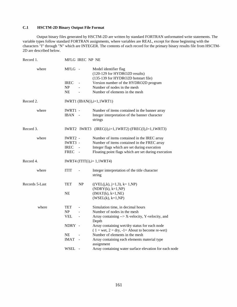
C.1 HSCTM-2D Binary Output File Format
Output binary files generated by HSCTM-2D are written by standard FORTRAN unformatted write statements. The variable types follow standard FORTRAN assignments, where variables are REAL, except for those beginning with the characters "I" through "N" which are INTEGER. The contents of each record for the primary binary results file from HSCTM2D are described below.
Record 1. MFLG IREC NP NE
where MFLG
IREC NP
-
--
Model identifier flag (120-129 for HYDRO2D results) (135-139 for HYDRO2D hotstart file) Version number of the HYDRO2D program Number of nodes in the mesh
NE - Number of elements in the mesh
Record 2. IWRT1 (IBAN(i),i=1,1WRT1)
where IWRT1 IBAN
--
Number of items contained in the banner array Integer interpretation of the banner character strings
Record 3. IWRT2 IWRT3 (IREC(i),i=1,1WRT2) (FREC(I),I=1,1WRT3)
where IWRT2 IWRT3 IREC FREC
----
Number of items contained in the IREC array Number of items contained in the FREC array Integer flags which are set during execution Floating point flags which are set during execution
Record 4. IWRT4 (ITIT(i),i= 1,1WRT4)
where ITIT - Integer interpretation of the title character string
Records 5-Last TET
NE
NP ((VEL(j,k), j=1,3), k= 1,NP) (NDRY(k), k=1,NP) (IMAT(k), k=1,NE) (WSEL(k), k=1,NP)
where TET NP
--
Simulation time, in decimal hours Number of nodes in the mesh
VEL
NDRY
NE
-
-
-
Array containing --> X-velocity, Y-velocity, and Depth Array containing wet/dry status for each node ( 1 = wet, 2 = dry, -1= About to become re-wet) Number of elements in the mesh
IMAT
WSEL
-
-
Array containing each elements material type assignment Array containing water surface elevation for each node
161

C.2 Card Image Input Data Coding Instructions for HYDRO2D
This description of input data is written in the language for a standard eight-column format in which the first three columns are reserved for "Card Group" and "Data Type" alpha- characters, respectively. These three columns are considered to be field 0. The rest of field 1, columns 4 through 8, is read in several combinations of columns. The instructions use the following syntax: "O,Cxx" where the "0" refers to field 0, "C" to the column and the "xx" are column numbers.
Of the cards shown in the following table, Network (mesh) data are prepared by GFGEN, an accompanying program that reads the geometry file generated by SMS and generates a binary file containing the finite element mesh that is read by HSCTM-2D. The other cards are prepared here. The sequence of cards should be in the order shown in Table C.1. Input variables are summarized in Table C.2.
Either free field or the standard eight-column card fields are permitted with the default being to free field. In standard eight column fields, unneeded variables can be omitted, but in free field unneeded variables are delimited by commas. Card image input is given in section C.3 following the input instructions for each card.
The first set of "B" cards will be used for the steady-state solution. This group of cards should be terminated by an "END" card. Dynamic boundary conditions for each time-step will then either be added to the basic input (boundary condition) file separated by "END" cards, or in a separate alternate boundary condition input file. All specified boundary conditions hold from one time step to another unless they are specifically modified. The program does not permit new boundary conditions to be specified in mid-run nor does it allow a change in the types (e.g., stage, discharge) of boundary conditions.
162

Table C.1
HYDRO2D Data Card Summary
Card Content Required
T1 - T2 TITLE CARDS NO
T3 TITLE CARD YES
$F FORMATTED DATA SET NO
$M MACHINE TYPE IDENTIFIER YES
$L INPUT/OUTPUT FILE NUMBERS NO
Sl SYSTEM INTERNATIONAL UNITS NO
CA SPECIAL CALCULATION VARIABLES NO
CO COMMENTS NO
DE WET/DRY BY ELEMENT NO
DM WET/DRY BY MARSH POROSITY NO
EV TURBULENT EXCHANGE AND MANNING'S N YES, if EX, COEFFICIENTS EY and HN are
not present
EX TURBULENT EXCHANGE COEFFICIENTS, X-PLANE NO
EY TURBULENT EXCHANGE COEFFICIENTS, Y-PLANE NO
FC FLOW CONTROL STRUCTURES NO
FD FLUID DENSITY NO
FT FLUID TEMPERATURE NO
G1 GEOMETRY, GENERAL GEOMETRY PARAMETERS NO
GC GEOMETRY, CONTINUITY CHECK LINES NO
GE GEOMETRY, ELEMENT CONNECTION TABLE NO
(continued)
163

Table C.1 (continued)
Card Content Required
GN GEOMETRY, NODAL COORDINATES, BOTTOM ELEVATIONS NO
GT GEOMETRY, ELEMENT TYPE (IMAT) NO
GV GEOMETRY, EDDY VISCOSITY TENSOR NO
GW GEOMETRY, 1-D CROSS SECTIONAL PROPERTIES NO
GY GEOMETRY, BOTTOM ELEVATIONS NO
HN HYDRAULICS, MANNING N-VALUES NO
IC INITIAL CONDITIONS, WATER-SURFACE ELEVATION YES
LAT LATITUDE NO
TI TIMING, NUMBER OF ITERATIONS COUNTER YES
TO TIMING FOR BINARY OUTPUT WRITE NO
TR TRACE PRINTOUT CONTROLS YES
TRN TRACE PRINTOUT NODE LIST NO
TZ TIMING, TIME ZERO YES
BCC BOUNDARY CONDITION CONTROL PARAMETERS NO
BA BOUNDARY, AZIMUTH OF FLOW *
BS BOUNDARY, CURRENT SPEED *
BH BOUNDARY, WATER-SURFACE ELEVATION *
BQ BOUNDARY, UNIT discharge *
(continued)
164
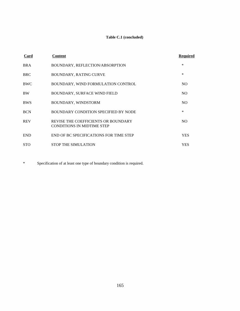
Table C.1 (concluded)
Card Content Required
BRA BOUNDARY, REFLECTION/ABSORPTION *
BRC BOUNDARY, RATING CURVE *
BWC BOUNDARY, WIND FORMULATION CONTROL NO
BW BOUNDARY, SURFACE WIND FIELD NO
BWS BOUNDARY, WINDSTORM NO
BCN BOUNDARY CONDITION SPECIFIED BY NODE *
REV REVISE THE COEFFICIENTS OR BOUNDARY NO CONDITIONS IN MIDTIME STEP
END END OF BC SPECIFICATIONS FOR TIME STEP YES
STO STOP THE SIMULATION YES
* Specification of at least one type of boundary condition is required.
165
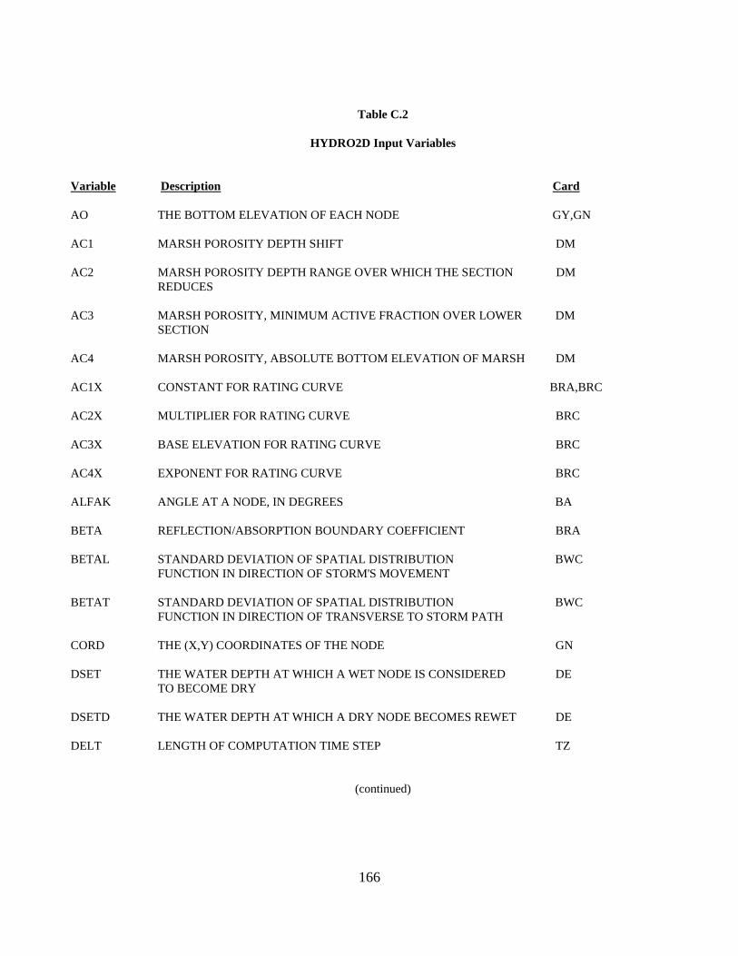
Table C.2
HYDRO2D Input Variables
Variable Description Card
AO THE BOTTOM ELEVATION OF EACH NODE GY,GN
AC1 MARSH POROSITY DEPTH SHIFT DM
AC2 MARSH POROSITY DEPTH RANGE OVER WHICH THE SECTION DM REDUCES
AC3 MARSH POROSITY, MINIMUM ACTIVE FRACTION OVER LOWER DM SECTION
AC4 MARSH POROSITY, ABSOLUTE BOTTOM ELEVATION OF MARSH DM
AC1X CONSTANT FOR RATING CURVE BRA,BRC
AC2X MULTIPLIER FOR RATING CURVE BRC
AC3X BASE ELEVATION FOR RATING CURVE BRC
AC4X EXPONENT FOR RATING CURVE BRC
ALFAK ANGLE AT A NODE, IN DEGREES BA
BETA REFLECTION/ABSORPTION BOUNDARY COEFFICIENT BRA
BETAL STANDARD DEVIATION OF SPATIAL DISTRIBUTION BWC FUNCTION IN DIRECTION OF STORM'S MOVEMENT
BETAT STANDARD DEVIATION OF SPATIAL DISTRIBUTION BWC FUNCTION IN DIRECTION OF TRANSVERSE TO STORM PATH
CORD THE (X,Y) COORDINATES OF THE NODE GN
DSET THE WATER DEPTH AT WHICH A WET NODE IS CONSIDERED DE TO BECOME DRY
DSETD THE WATER DEPTH AT WHICH A DRY NODE BECOMES REWET DE
DELT LENGTH OF COMPUTATION TIME STEP TZ
(continued)
166

Table C.2 (continued)
Variable Description Card
ELEV THE AVERAGE INITIAL WATER-SURFACE ELEVATION OVER IC THE MESH
FLD ANY ALPHANUMERIC USER COMMENT CO,END
FLZ3 FLOW CONTROL EQUATION, BASE FLOW FC
FLZ4 FLOW CONTROL EQUATION, RELATIONAL COEFFICIENT FC
FLZ5 FLOW CONTROL EQUATION, REFERENCE ELEVATION OR HEAD FC DIFFERENCE
FLZ6 FLOW CONTROL EQUATION, EXPONENT FC
FLZ7 FLOW CONTROL EQUATION, DIRECTION OF FLOW FC (RADIANS COUNTERCLOCKWISE FROM + X-AXIS)
HFX HEAD SPECIFICATION ALONG A CONTINUITY LINE BH
HMIN INITIAL DEPTH FOR ONE DIMENSIONAL ELEMENTS IC
IBUP LOGICAL UNIT NUMBER FOR DYNAMIC BOUNDARY CONDITIONS $L INPUT TO HYDRO2D
IC1 CARD GROUP IDENTIFIER, ALL CARDS ALL
IC3 DATA TYPE IDENTIFIER, SOME CARDS SOME
ICON CONTINUITY LINE NUMBER BRA
ICOMID (IVRSID) COMPUTER IDENTIFIER $M
IDEN DYNAMIC COUNTER FOR INPUT OF VARIABLE (self count) FD
ISTYPE STORM REFERENCE POINT BWS
DMN NODAL MARSH POROSITY SWITCH DM
IDNOPT MARSH OPTION SWITCH DM
(continued)
167
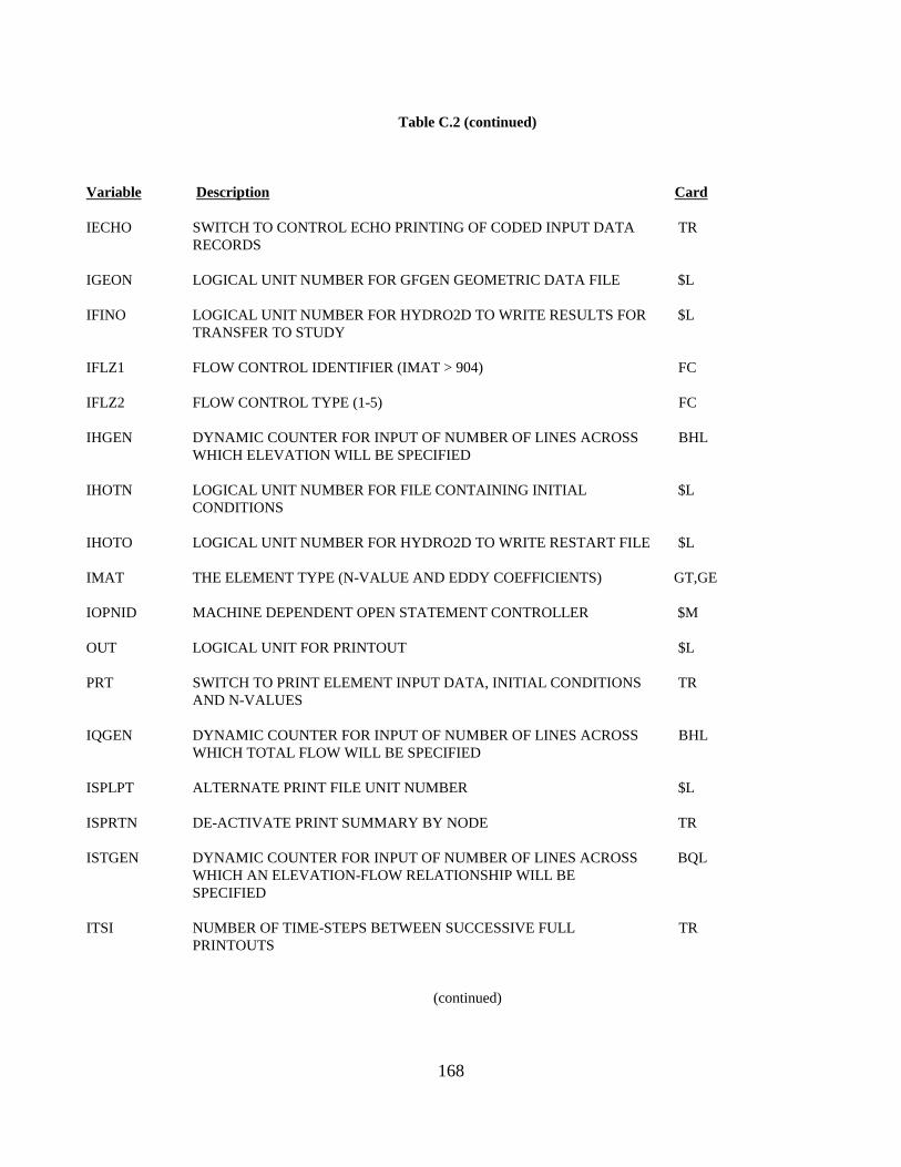
Table C.2 (continued)
Variable Description Card
IECHO SWITCH TO CONTROL ECHO PRINTING OF CODED INPUT DATA TR RECORDS
IGEON LOGICAL UNIT NUMBER FOR GFGEN GEOMETRIC DATA FILE $L
IFINO LOGICAL UNIT NUMBER FOR HYDRO2D TO WRITE RESULTS FOR $L TRANSFER TO STUDY
IFLZ1 FLOW CONTROL IDENTIFIER (IMAT > 904) FC
IFLZ2 FLOW CONTROL TYPE (1-5) FC
IHGEN DYNAMIC COUNTER FOR INPUT OF NUMBER OF LINES ACROSS BHL WHICH ELEVATION WILL BE SPECIFIED
IHOTN LOGICAL UNIT NUMBER FOR FILE CONTAINING INITIAL $L CONDITIONS
IHOTO LOGICAL UNIT NUMBER FOR HYDRO2D TO WRITE RESTART FILE $L
IMAT THE ELEMENT TYPE (N-VALUE AND EDDY COEFFICIENTS) GT,GE
IOPNID MACHINE DEPENDENT OPEN STATEMENT CONTROLLER $M
OUT LOGICAL UNIT FOR PRINTOUT $L
PRT SWITCH TO PRINT ELEMENT INPUT DATA, INITIAL CONDITIONS TR AND N-VALUES
IQGEN DYNAMIC COUNTER FOR INPUT OF NUMBER OF LINES ACROSS BHL WHICH TOTAL FLOW WILL BE SPECIFIED
ISPLPT ALTERNATE PRINT FILE UNIT NUMBER $L
ISPRTN DE-ACTIVATE PRINT SUMMARY BY NODE TR
ISTGEN DYNAMIC COUNTER FOR INPUT OF NUMBER OF LINES ACROSS BQL WHICH AN ELEVATION-FLOW RELATIONSHIP WILL BE SPECIFIED
ITSI NUMBER OF TIME-STEPS BETWEEN SUCCESSIVE FULL TR PRINTOUTS
(continued)
168
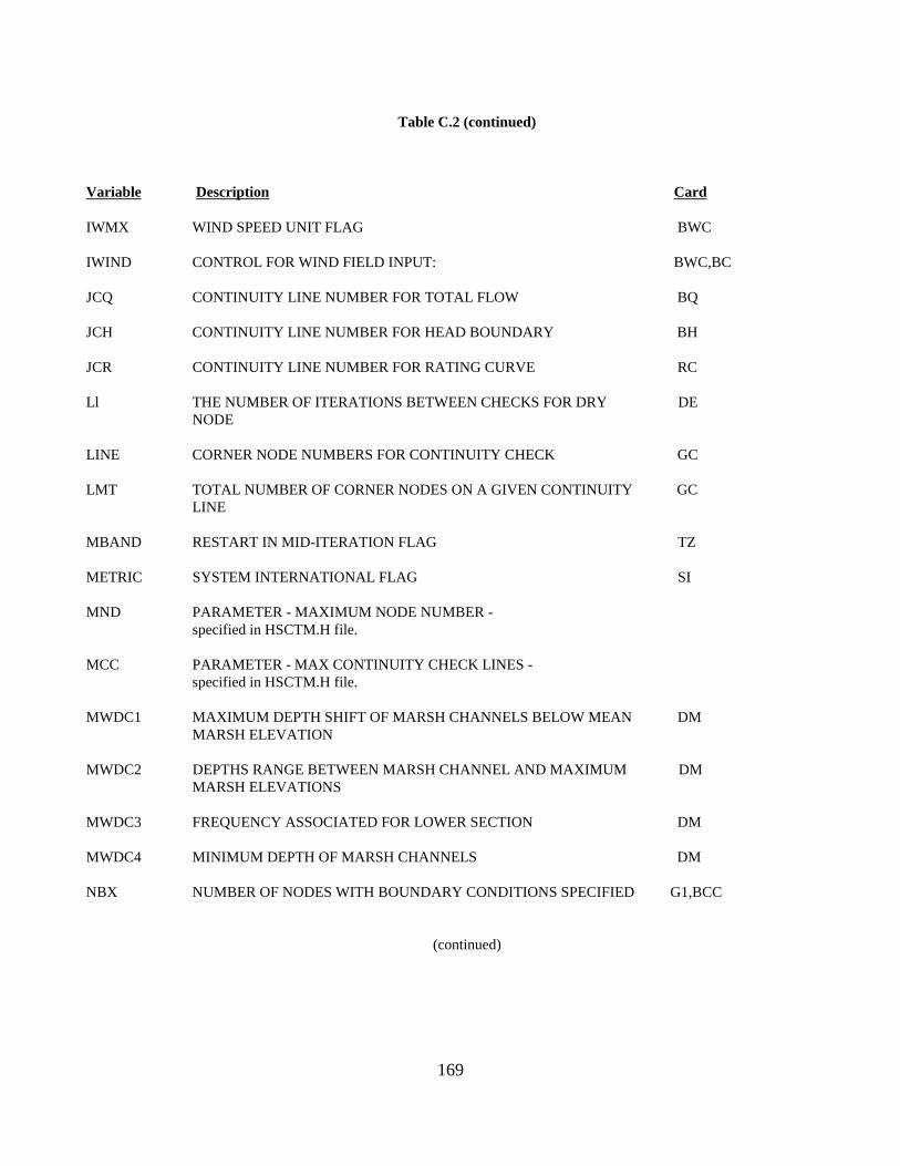
Table C.2 (continued)
Variable Description Card
IWMX WIND SPEED UNIT FLAG BWC
IWIND CONTROL FOR WIND FIELD INPUT: BWC,BC
JCQ CONTINUITY LINE NUMBER FOR TOTAL FLOW BQ
JCH CONTINUITY LINE NUMBER FOR HEAD BOUNDARY BH
JCR CONTINUITY LINE NUMBER FOR RATING CURVE RC
Ll THE NUMBER OF ITERATIONS BETWEEN CHECKS FOR DRY DE NODE
LINE CORNER NODE NUMBERS FOR CONTINUITY CHECK GC
LMT TOTAL NUMBER OF CORNER NODES ON A GIVEN CONTINUITY GC LINE
MBAND RESTART IN MID-ITERATION FLAG TZ
METRIC SYSTEM INTERNATIONAL FLAG SI
MND PARAMETER - MAXIMUM NODE NUMBER specified in HSCTM.H file.
MCC PARAMETER - MAX CONTINUITY CHECK LINES specified in HSCTM.H file.
MWDC1 MAXIMUM DEPTH SHIFT OF MARSH CHANNELS BELOW MEAN DM MARSH ELEVATION
MWDC2 DEPTHS RANGE BETWEEN MARSH CHANNEL AND MAXIMUM DM MARSH ELEVATIONS
MWDC3 FREQUENCY ASSOCIATED FOR LOWER SECTION DM
MWDC4 MINIMUM DEPTH OF MARSH CHANNELS DM
NBX NUMBER OF NODES WITH BOUNDARY CONDITIONS SPECIFIED G1,BCC
(continued)
169
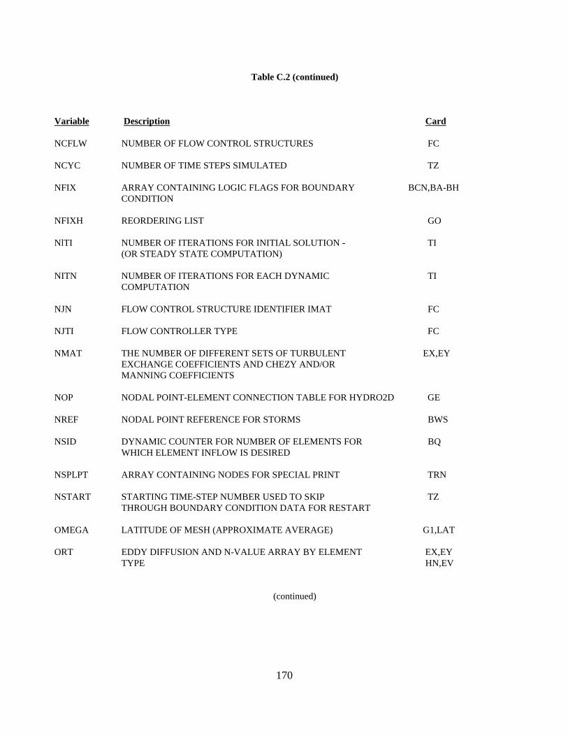
Table C.2 (continued)
Variable Description Card
NCFLW NUMBER OF FLOW CONTROL STRUCTURES FC
NCYC NUMBER OF TIME STEPS SIMULATED TZ
NFIX ARRAY CONTAINING LOGIC FLAGS FOR BOUNDARY BCN,BA-BH CONDITION
NFIXH REORDERING LIST GO
NlTI NUMBER OF ITERATIONS FOR INITIAL SOLUTION TI (OR STEADY STATE COMPUTATION)
NITN NUMBER OF ITERATIONS FOR EACH DYNAMIC TI COMPUTATION
NJN FLOW CONTROL STRUCTURE IDENTIFIER IMAT FC
NJTI FLOW CONTROLLER TYPE FC
NMAT THE NUMBER OF DIFFERENT SETS OF TURBULENT EX,EY EXCHANGE COEFFICIENTS AND CHEZY AND/OR MANNING COEFFICIENTS
NOP NODAL POINT-ELEMENT CONNECTION TABLE FOR HYDRO2D GE
NREF NODAL POINT REFERENCE FOR STORMS BWS
NSID DYNAMIC COUNTER FOR NUMBER OF ELEMENTS FOR BQ WHICH ELEMENT INFLOW IS DESIRED
NSPLPT ARRAY CONTAINING NODES FOR SPECIAL PRINT TRN
NSTART STARTING TIME-STEP NUMBER USED TO SKIP TZ THROUGH BOUNDARY CONDITION DATA FOR RESTART
OMEGA LATITUDE OF MESH (APPROXIMATE AVERAGE) G1,LAT
ORT EDDY DIFFUSION AND N-VALUE ARRAY BY ELEMENT EX,EY TYPE HN,EV
(continued)
170

Table C.2 (continued)
Variable Description Card
QF TOTAL FLOW ALONG A CONTINUITY LINE BQ
QDIR FLOW DIRECTION ALONG CONTINUITY LINE BQ
QTOT TOTAL DISCHARGE (CFS) CROSSING A CONTINUITY LINE BQ
QVEC THE UNIT DISCHARGE (CFS/FT) BQ
RON THE ARRAY OF NODAL FLUID DENSITY FD
SIDF ELEMENT INFLOW (PER UNIT AREA) BQ
SPEC ARRAY CONTAINING BOUNDARY CONDITION BCN, SPECIFICATIONS BA-BH
SS1 LEFT SIDE SLOPE FOR ONE DIMENSIONAL NODES GW
SS2 RIGHT SIDE SLOPE FOR ONE DIMENSIONAL NODES GW
SSDCRT STEADY STATE SATISFACTORY DEPTH CRITION TI
SSWSE STEADY STATE WATER SURFACE ELEVATION BRC
TAX WIND DIRECTION (DEGREES COUNTERCLOCKWISE BW FROM + X-AXIS)
TBINRY ARRAY CONTAINING USER SELECTED HOURS TO SAVE TO TO BINARY FINAL RESULTS FILE
TEMP AVERAGE INITIAL WATER TEMPERATURE FT
TH AZIMUTH OF X-DIRECTION OF AN ELEMENT FOR GE,GV SPECIFYING EDDY DIFFUSION COEFFICIENTS
THETA DIRECTION OF FLOW (RADIANS MEASURED BQ,BRA COUNTERCLOCKWISE) BRC
THETAK ORIENTATION OF STORM BWS
THETAS DIRECTION OF STORM TRACK BWS
(continued)
171
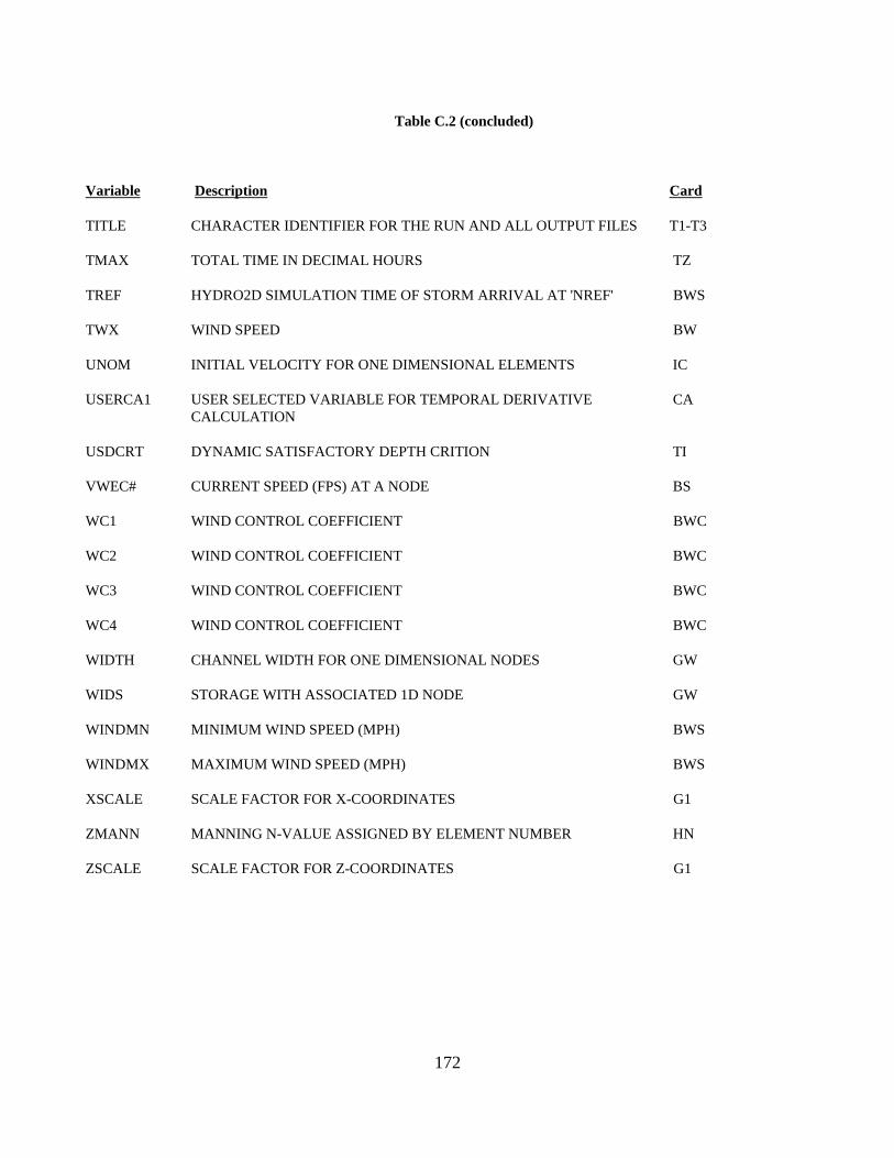
Variable
TITLE
TMAX
TREF
TWX
UNOM
USERCA1
USDCRT
VWEC#
WC1
WC2
WC3
WC4
WIDTH
WIDS
WINDMN
WINDMX
XSCALE
ZMANN
ZSCALE
Table C.2 (concluded)
Description Card
CHARACTER IDENTIFIER FOR THE RUN AND ALL OUTPUT FILES T1-T3
TOTAL TIME IN DECIMAL HOURS TZ
HYDRO2D SIMULATION TIME OF STORM ARRIVAL AT 'NREF' BWS
WIND SPEED BW
INITIAL VELOCITY FOR ONE DIMENSIONAL ELEMENTS IC
USER SELECTED VARIABLE FOR TEMPORAL DERIVATIVE CA CALCULATION
DYNAMIC SATISFACTORY DEPTH CRITION TI
CURRENT SPEED (FPS) AT A NODE BS
WIND CONTROL COEFFICIENT BWC
WIND CONTROL COEFFICIENT BWC
WIND CONTROL COEFFICIENT BWC
WIND CONTROL COEFFICIENT BWC
CHANNEL WIDTH FOR ONE DIMENSIONAL NODES GW
STORAGE WITH ASSOCIATED 1D NODE GW
MINIMUM WIND SPEED (MPH) BWS
MAXIMUM WIND SPEED (MPH) BWS
SCALE FACTOR FOR X-COORDINATES G1
MANNING N-VALUE ASSIGNED BY ELEMENT NUMBER HN
SCALE FACTOR FOR Z-COORDINATES G1
172
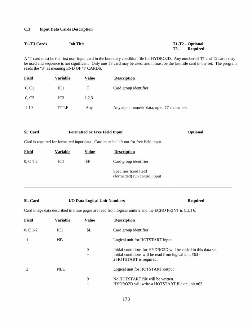
____________________________________________________________________________________________________
____________________________________________________________________________________________________
C.3 Input Data Cards Description
T1-T3 Cards Job Title T1-T2 - Optional T3 - Required
A 'T' card must be the first user input card in the boundary condition file for HYDRO2D. Any number of T1 and T2 cards may be used and sequence is not significant. Only one T3 card may be used, and it must be the last title card in the set. The program reads the "3" as meaning END OF 'T' CARDS.
Field Variable Value Description
0, C1 IC1 T Card group identifier
0, C2 IC3 1,2,3
1-10 TITLE Any Any alpha-numeric data, up to 77 characters.
$F Card Formatted or Free Field Input Optional
Card is required for formatted input data. Card must be left out for free field input.
Field Variable Value Description
0, C 1-2 IC1 $F Card group identifier
Specifies fixed field (formatted) run control input
$L Card I/O Data Logical Unit Numbers Required
Card image data described in these pages are read from logical unit# 2 and the ECHO PRINT is (LU) 6.
Field Variable Value Description
0, C 1-2 IC1 $L
1 NB
0 +
2 NLL
0
Card group identifier
Logical unit for HOTSTART input
Initial conditions for HYDRO2D will be coded in this data set.Initial conditions will be read from logical unit #63 a HOTSTART is required.
Logical unit for HOTSTART output
No HOTSTART file will be written. + HYDRO2D will write a HOTSTART file on unit #62.
173
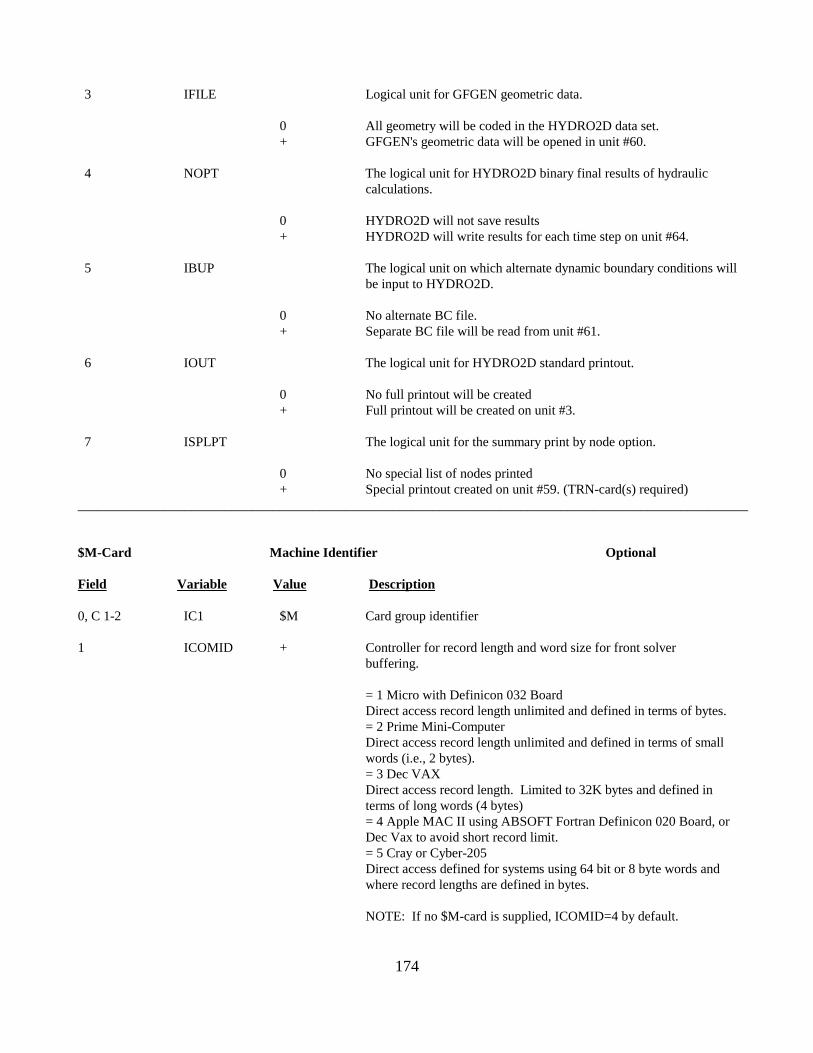
____________________________________________________________________________________________________
3 IFILE Logical unit for GFGEN geometric data.
0 +
All geometry will be coded in the HYDRO2D data set.GFGEN's geometric data will be opened in unit #60.
4 NOPT The logical unit for HYDRO2D binary final results of hydraulic calculations.
0 +
HYDRO2D will not save resultsHYDRO2D will write results for each time step on unit #64.
5 IBUP The logical unit on which alternate dynamic boundary conditions will be input to HYDRO2D.
0 +
No alternate BC file.Separate BC file will be read from unit #61.
6 IOUT The logical unit for HYDRO2D standard printout.
0 +
No full printout will be createdFull printout will be created on unit #3.
7 ISPLPT The logical unit for the summary print by node option.
0 +
No special list of nodes printedSpecial printout created on unit #59. (TRN-card(s) required)
$M-Card Machine Identifier Optional
Field Variable Value Description
0, C 1-2 IC1 $M Card group identifier
1 ICOMID + Controller for record length and word size for front solver buffering.
= 1 Micro with Definicon 032 Board Direct access record length unlimited and defined in terms of bytes. = 2 Prime Mini-Computer Direct access record length unlimited and defined in terms of small words (i.e., 2 bytes). = 3 Dec VAX Direct access record length. Limited to 32K bytes and defined in terms of long words (4 bytes) = 4 Apple MAC II using ABSOFT Fortran Definicon 020 Board, or Dec Vax to avoid short record limit. = 5 Cray or Cyber-205 Direct access defined for systems using 64 bit or 8 byte words and where record lengths are defined in bytes.
NOTE: If no $M-card is supplied, ICOMID=4 by default.
174
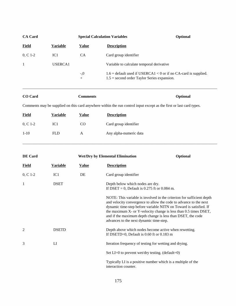
____________________________________________________________________________________________________
____________________________________________________________________________________________________
CA Card Special Calculation Variables Optional
Field Variable Value Description
0, C 1-2 IC1 CA Card group identifier
1 USERCA1 Variable to calculate temporal derivative
-,0 1.6 = default used if USERCA1 < 0 or if no CA-card is supplied. + 1.5 = second order Taylor Series expansion.
CO Card Comments Optional
Comments may be supplied on this card anywhere within the run control input except as the first or last card types.
Field Variable Value Description
0, C 1-2 IC1 CO Card group identifier
1-10 FLD A Any alpha-numeric data
DE Card Wet/Dry by Elemental Elimination Optional
Field Variable Value Description
0, C 1-2 IC1 DE Card group identifier
1 DSET Depth below which nodes are dry. If DSET = 0, Default is 0.275 ft or 0.084 m.
NOTE: This variable is involved in the criterion for sufficient depth and velocity convergence to allow the code to advance to the next dynamic time-step before variable NITN on Toward is satisfied. If the maximum X- or Y-velocity change is less than 0.5 times DSET, and if the maximum depth change is less than DSET, the code advances to the next dynamic time-step.
2 DSETD Depth above which nodes become active when rewetting. If DSETD=0, Default is 0.60 ft or 0.183 m
3 LI Iteration frequency of testing for wetting and drying.
Set LI=0 to prevent wet/dry testing. (default=0)
Typically LI is a positive number which is a multiple of the interaction counter.
175
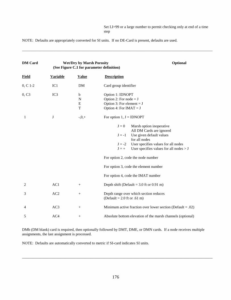
____________________________________________________________________________________________________
____________________________________________________________________________________________________
Set LI=99 or a large number to permit checking only at end of a time step
NOTE: Defaults are appropriately converted for SI units. If no DE-Card is present, defaults are used.
DM Card Wet/Dry by Marsh Porosity Optional (See Figure C.1 for parameter definition)
Field Variable Value Description
0, C 1-2 IC1 DM Card group identifier
0, C3 IC3 b Option 1: IDNOPT N Option 2: For node = J E Option 3: For element = J T Option 4: For IMAT = J
1 J -,0,+ For option 1, J = IDNOPT
J = 0 Marsh option inoperative All DM Cards are ignored
J = -1 Use given default values for all nodes
J = -2 User specifies values for all nodes J = + User specifies values for all nodes > J
For option 2, code the node number
For option 3, code the element number
For option 4, code the IMAT number
2 AC1 + Depth shift (Default = 3.0 ft or 0.91 m)
3 AC2 + Depth range over which section reduces (Default = 2.0 ft or .61 m)
4 AC3 + Minimum active fraction over lower section (Default = .02)
5 AC4 + Absolute bottom elevation of the marsh channels (optional)
DMb (DM blank) card is required, then optionally followed by DMT, DME, or DMN cards. If a node receives multiple assignments, the last assignment is processed.
NOTE: Defaults are automatically converted to metric if SI-card indicates SI units.
176

EV Card Turbulent Exchange Coefficients and Manning's N Required if HN, EX, or EY not used
Turbulent exchange coefficients should be coded by element type. In equation notation the value for Exx, Exy, Eyx, Eyy and Manning's n are coded on this card.
Field Variable Value Description
0, C 1-2 IC1 EV Card group identifier
1 J + Element type number for the set of turbulent exchange coefficients (IMAT)
2 ORT(J,1) + Exx = x-momentum turbulent exchange in x-direction (Ib-sec/ft2 or Pascal-sec for SI-units)
3 ORT(J,2) + Exy = x-momentum turbulent exchange in y-direction (lb-sec/ft2 or Pascal-sec for SI-units)
4 ORT(J,3) + Eyx = y-momentum turbulent exchange in x-direction (lb-sec/ft2 or Pascal-sec for SI-units)
5 ORT(J,4) + Eyy = y-momentum turbulent exchange in y-direction (lb-sec/ft2 or Pascal-sec for SI-units)
6 ORT(J,5) + Manning's Coefficient (or Chezy if ORT(J,5) > 3.0)
Recall the formula for Peclet numbers (P), where P is recommended to be less than 20.
P = u dx (1.94) E
where:u = stream wise velocity (fps)dx = length of element in stream wise direction (ft)E = eddy viscosity (Ib-sec/ft2)1.94 required for non-SI calculation
177
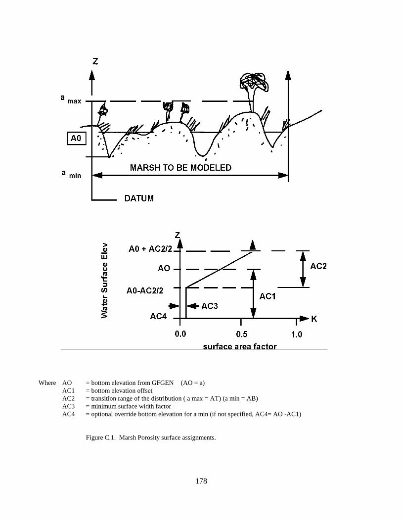
Where AO = bottom elevation from GFGEN (AO = a) AC1 = bottom elevation offset AC2 = transition range of the distribution ( a max = AT) (a min = AB) AC3 = minimum surface width factor AC4 = optional override bottom elevation for a min (if not specified, AC4= AO -AC1)
Figure C.1. Marsh Porosity surface assignments.
178
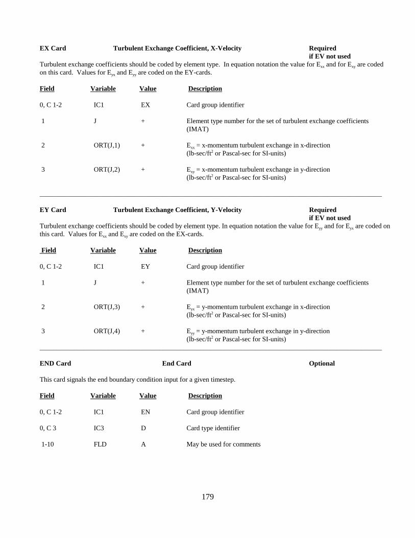
____________________________________________________________________________________________________
____________________________________________________________________________________________________
EX Card Turbulent Exchange Coefficient, X-Velocity Required if EV not used
Turbulent exchange coefficients should be coded by element type. In equation notation the value for Exx and for Exy are coded on this card. Values for E and E are coded on the EY-cards. yx yy
Field Variable Value Description
0, C 1-2 IC1 EX Card group identifier
1 J + Element type number for the set of turbulent exchange coefficients (IMAT)
2 ORT(J,1) + Exx = x-momentum turbulent exchange in x-direction (lb-sec/ft2 or Pascal-sec for SI-units)
3 ORT(J,2) + Exy = x-momentum turbulent exchange in y-direction (lb-sec/ft2 or Pascal-sec for SI-units)
EY Card Turbulent Exchange Coefficient, Y-Velocity Required if EV not used
Turbulent exchange coefficients should be coded by element type. In equation notation the value for Eyy and for E are coded onyx
this card. Values for Exx and Exy are coded on the EX-cards.
Field Variable Value Description
0, C 1-2 IC1 EY Card group identifier
1 J + Element type number for the set of turbulent exchange coefficients (IMAT)
2 ORT(J,3) + Eyx = y-momentum turbulent exchange in x-direction (lb-sec/ft2 or Pascal-sec for SI-units)
3 ORT(J,4) + Eyy = y-momentum turbulent exchange in y-direction (lb-sec/ft2 or Pascal-sec for SI-units)
END Card End Card Optional
This card signals the end boundary condition input for a given timestep.
Field Variable Value Description
0, C 1-2 IC1 EN
0, C 3 IC3 D
1-10 FLD A
Card group identifier
Card type identifier
May be used for comments
179
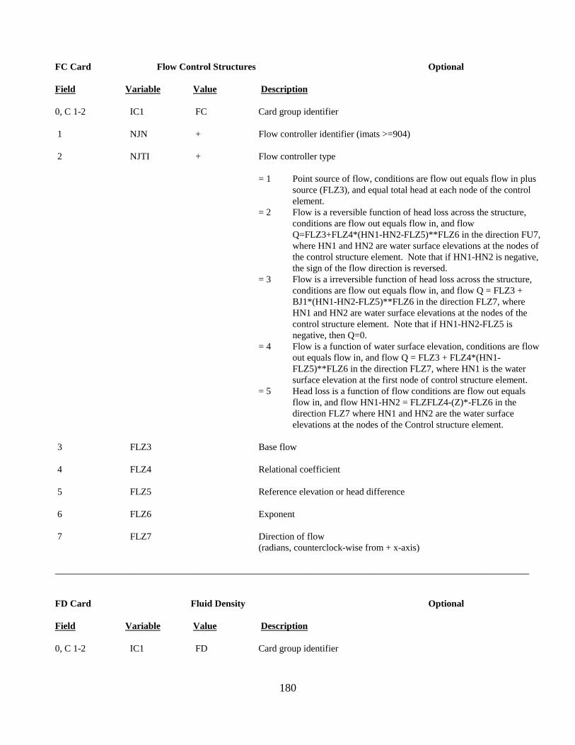
____________________________________________________________________________________________________
FC Card Flow Control Structures Optional
Field Variable Value Description
0, C 1-2 IC1 FC Card group identifier
1 NJN + Flow controller identifier (imats >=904)
2 NJTI + Flow controller type
= 1 Point source of flow, conditions are flow out equals flow in plus source (FLZ3), and equal total head at each node of the control element.
= 2 Flow is a reversible function of head loss across the structure, conditions are flow out equals flow in, and flow Q=FLZ3+FLZ4*(HN1-HN2-FLZ5)**FLZ6 in the direction FU7, where HN1 and HN2 are water surface elevations at the nodes of the control structure element. Note that if HN1-HN2 is negative, the sign of the flow direction is reversed.
= 3 Flow is a irreversible function of head loss across the structure, conditions are flow out equals flow in, and flow Q = FLZ3 + BJ1*(HN1-HN2-FLZ5)**FLZ6 in the direction FLZ7, where HN1 and HN2 are water surface elevations at the nodes of the control structure element. Note that if HN1-HN2-FLZ5 is negative, then Q=0.
= 4 Flow is a function of water surface elevation, conditions are flow out equals flow in, and flow Q = FLZ3 + FLZ4*(HN1-FLZ5)**FLZ6 in the direction FLZ7, where HN1 is the water surface elevation at the first node of control structure element.
= 5 Head loss is a function of flow conditions are flow out equals flow in, and flow HN1-HN2 = FLZFLZ4-(Z)*-FLZ6 in the direction FLZ7 where HN1 and HN2 are the water surface elevations at the nodes of the Control structure element.
3 FLZ3 Base flow
4 FLZ4 Relational coefficient
5 FLZ5 Reference elevation or head difference
6 FLZ6 Exponent
7 FLZ7 Direction of flow (radians, counterclock-wise from + x-axis)
FD Card Fluid Density Optional
Field Variable Value Description
0, C 1-2 IC1 FD Card group identifier
180
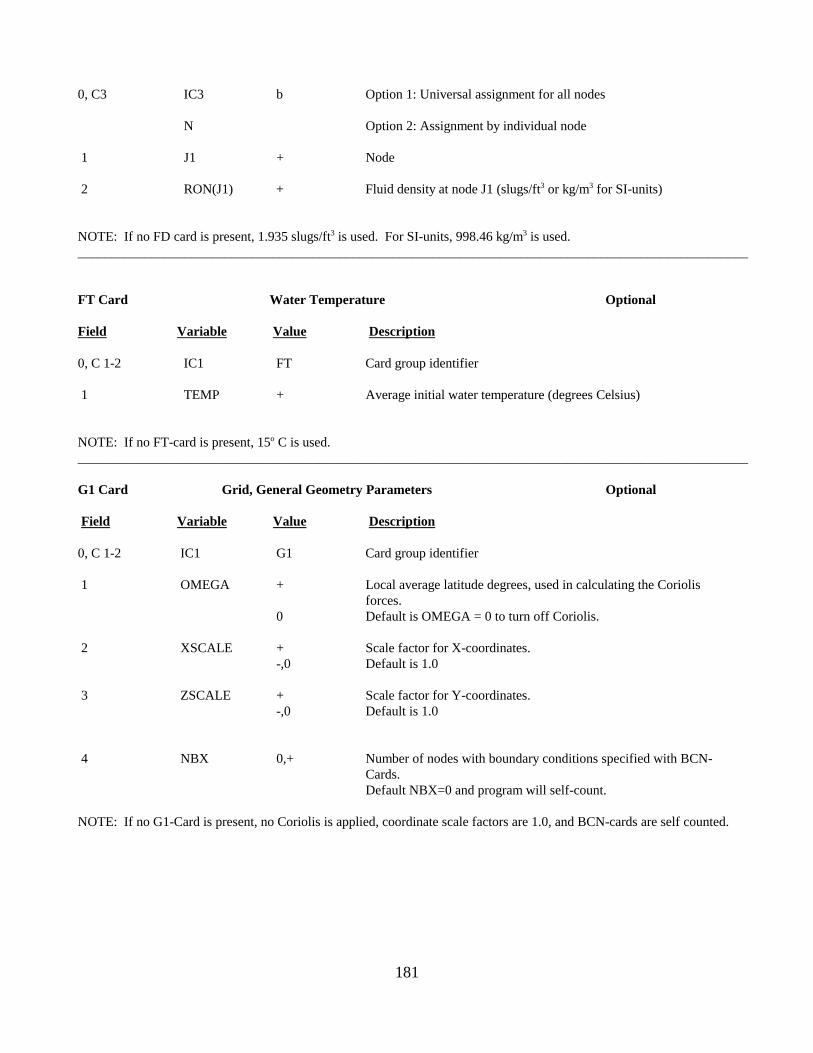
____________________________________________________________________________________________________
____________________________________________________________________________________________________
0, C3 IC3 b
N
1 J1 +
2 RON(J1) +
Option 1: Universal assignment for all nodes
Option 2: Assignment by individual node
Node
Fluid density at node J1 (slugs/ft3 or kg/m3 for SI-units)
NOTE: If no FD card is present, 1.935 slugs/ft3 is used. For SI-units, 998.46 kg/m3 is used.
FT Card Water Temperature Optional
Field Variable Value Description
0, C 1-2 IC1 FT Card group identifier
1 TEMP + Average initial water temperature (degrees Celsius)
NOTE: If no FT-card is present, 15o C is used.
G1 Card Grid, General Geometry Parameters Optional
Field Variable Value Description
0, C 1-2 IC1 G1
1 OMEGA +
0
2 XSCALE + -,0
3 ZSCALE + -,0
Card group identifier
Local average latitude degrees, used in calculating the Coriolisforces. Default is OMEGA = 0 to turn off Coriolis.
Scale factor for X-coordinates.Default is 1.0
Scale factor for Y-coordinates.Default is 1.0
4 NBX 0,+ Number of nodes with boundary conditions specified with BCN-Cards. Default NBX=0 and program will self-count.
NOTE: If no G1-Card is present, no Coriolis is applied, coordinate scale factors are 1.0, and BCN-cards are self counted.
181
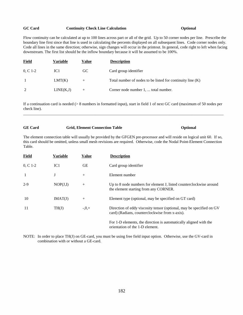
____________________________________________________________________________________________________
GC Card Continuity Check Line Calculation Optional
Flow continuity can be calculated at up to 100 lines across part or all of the grid. Up to 50 corner nodes per line. Prescribe the boundary line first since that line is used in calculating the percents displayed on all subsequent lines. Code corner nodes only. Code all lines in the same direction; otherwise, sign changes will occur in the printout. In general, code right to left when facing downstream. The first list should be the inflow boundary because it will be assumed to be 100%.
Field Variable Value Description
0, C 1-2 IC1 GC
1 LMT(K) +
2 LINE(K,J) +
Card group identifier
Total number of nodes to be listed for continuity line (K)
Corner node number 1, ... total number.
If a continuation card is needed (> 8 numbers in formatted input), start in field 1 of next GC card (maximum of 50 nodes per check line).
GE Card Grid, Element Connection Table Optional
The element connection table will usually be provided by the GFGEN pre-processor and will reside on logical unit 60. If so, this card should be omitted, unless small mesh revisions are required. Otherwise, code the Nodal Point-Element Connection Table.
Field Variable Value Description
0, C 1-2 IC1 GE Card group identifier
1 J + Element number
2-9 NOP(J,I) + Up to 8 node numbers for element J, listed counterclockwise around the element starting from any CORNER.
10 IMAT(J) + Element type (optional, may be specified on GT card)
11 TH(J) -,0,+ Direction of eddy viscosity tensor (optional, may be specified on GV card) (Radians, counterclockwise from x-axis).
For 1-D elements, the direction is automatically aligned with the orientation of the 1-D element.
NOTE: In order to place TH(J) on GE-card, you must be using free field input option. Otherwise, use the GV-card in combination with or without a GE-card.
182
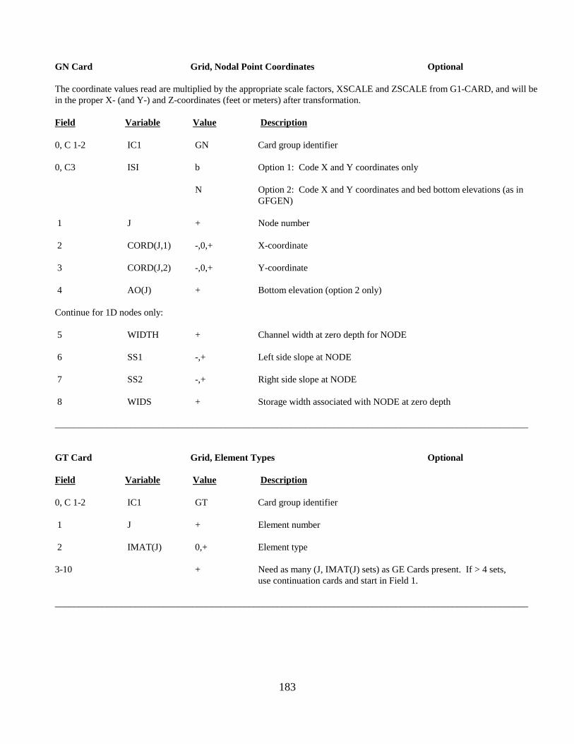
____________________________________________________________________________________________________
____________________________________________________________________________________________________
GN Card Grid, Nodal Point Coordinates Optional
The coordinate values read are multiplied by the appropriate scale factors, XSCALE and ZSCALE from G1-CARD, and will be in the proper X- (and Y-) and Z-coordinates (feet or meters) after transformation.
Field Variable Value Description
0, C 1-2 IC1 GN Card group identifier
0, C3 ISI b Option 1: Code X and Y coordinates only
N Option 2: Code X and Y coordinates and bed bottom elevations (as in GFGEN)
1 J + Node number
2 CORD(J,1) -,0,+ X-coordinate
3 CORD(J,2) -,0,+ Y-coordinate
4 AO(J) + Bottom elevation (option 2 only)
Continue for 1D nodes only:
5 WIDTH + Channel width at zero depth for NODE
6 SS1 -,+ Left side slope at NODE
7 SS2 -,+ Right side slope at NODE
8 WIDS + Storage width associated with NODE at zero depth
GT Card Grid, Element Types Optional
Field Variable Value Description
0, C 1-2 IC1 GT
1 J +
2 IMAT(J) 0,+
3-10 +
Card group identifier
Element number
Element type
Need as many (J, IMAT(J) sets) as GE Cards present. If > 4 sets, use continuation cards and start in Field 1.
183
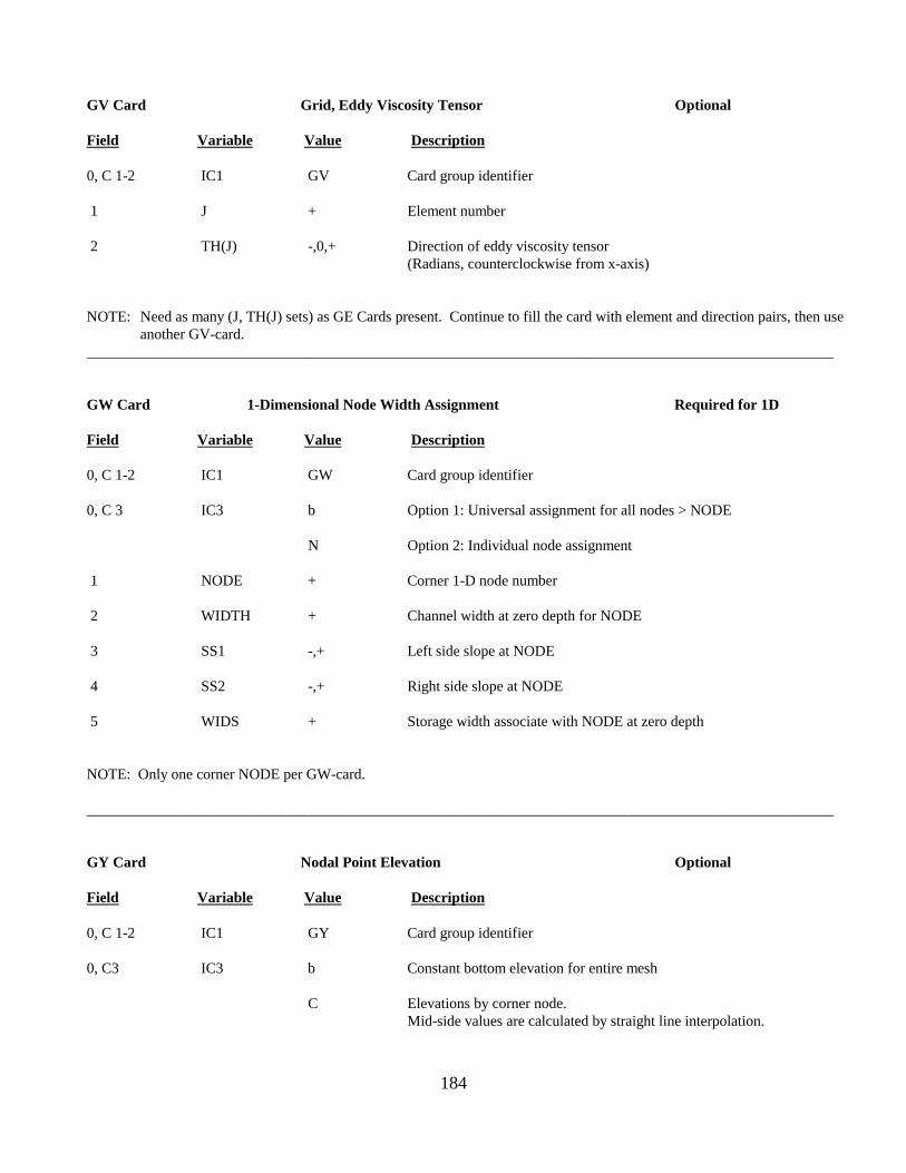
____________________________________________________________________________________________________
____________________________________________________________________________________________________
GV Card Grid, Eddy Viscosity Tensor Optional
Field Variable Value Description
0, C 1-2 IC1 GV
1 J +
2 TH(J) -,0,+
Card group identifier
Element number
Direction of eddy viscosity tensor (Radians, counterclockwise from x-axis)
NOTE: Need as many (J, TH(J) sets) as GE Cards present. Continue to fill the card with element and direction pairs, then use another GV-card.
GW Card 1-Dimensional Node Width Assignment Required for 1D
Field Variable Value Description
0, C 1-2 IC1 GW
0, C 3 IC3 b
N
1 NODE +
2 WIDTH +
3 SS1 -,+
4 SS2 -,+
5 WIDS +
Card group identifier
Option 1: Universal assignment for all nodes > NODE
Option 2: Individual node assignment
Corner 1-D node number
Channel width at zero depth for NODE
Left side slope at NODE
Right side slope at NODE
Storage width associate with NODE at zero depth
NOTE: Only one corner NODE per GW-card.
GY Card Nodal Point Elevation Optional
Field Variable Value Description
0, C 1-2 IC1 GY
0, C3 IC3 b
C
Card group identifier
Constant bottom elevation for entire mesh
Elevations by corner node. Mid-side values are calculated by straight line interpolation.
184
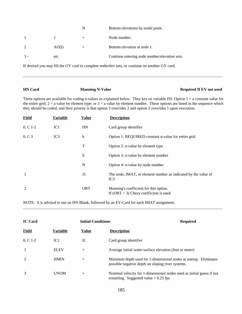
____________________________________________________________________________________________________
____________________________________________________________________________________________________
N Bottom elevations by nodal point.
1 1 + Node number.
2 AO(I) + Bottom elevation at node 1.
3 - etc. Continue entering node number/elevation sets.
If desired you may fill the GY card in complete node/elev sets, or continue on another GY card.
HN Card Manning N-Value Required If EV not used
Three options are available for coding n-values as explained below. They key on variable ISI: Option 1 = a constant value for the entire grid; 2 = a value by element type; or 3 = a value by element number. These options are listed in the sequence which they should be coded, and their priority is that option 3 overrides 2 and option 2 overrides 1 upon execution.
Field Variable Value Description
0, C 1-2 IC1 HN Card group identifier
0, C 3 IC3 b Option 1: REQUIRED constant n-value for entire grid
T Option 2: n-value by element type
E Option 3: n-value by element number
N Option 4: n-value by node number
1 J1 The node, IMAT, or element number as indicated by the value of IC3
2 ORT Manning's coefficient for this option. If (ORT > 3) Chezy coefficient is used
NOTE: It is advised to use an HN-Blank, followed by an EV-Card for each IMAT assignment.
IC Card Initial Conditions Required
Field Variable Value Description
0, C 1-2 IC1 IC Card group identifier
1 ELEV + Average initial water-surface elevation (feet or meter)
2 HMIN + Minimum depth used for 1-dimensional nodes at startup. Eliminates possible negative depth on sloping river systems.
3 UNOM + Nominal velocity for 1-dimensional nodes used as initial guess if not restarting. Suggested value = 0.25 fps
185
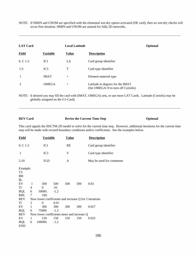
____________________________________________________________________________________________________
____________________________________________________________________________________________________
NOTE: If HMIN and UNOM are specified with the elemental wet-dry option activated (DE card), then no wet-dry checks will occur first iteration. HMIN and UNOM are unused for fully 2D networks.
LAT Card Local Latitude Optional
Field Variable Value Description
0, C 1-2 IC1 LA Card group identifier
C3 IC3 T Card type identifier
1 IMAT + Element material type
2 OMEGA + Latitude in degrees for the IMAT (Set OMEGA=0 to turn off Coriolis)
NOTE: It desired you may fill the card with (IMAT, OMEGA) sets, or use more LAT Cards. Latitude (Coriolis) may be globally assigned on the G1-Card).
REV Card Revise the Current Time Step Optional
This card signals the HSCTM-2D model to solve for the current time step. However, additional iterations for the current time step will be made with revised boundary conditions and/or coefficients. See the examples below.
Field Variable Value Description
0, C 1-2 IC1 RE Card group identifier
1 IC3 V Card type identifier
2-10 FLD A May be used for comments
Example: T3 $M $L EV 1 500 500 500 500 0.03 Tl 4 0 .01 BQL 6 50000. -1.2 BHL 7 100. REV Now lower coefficients and increase Q for 2 iterations Tl 2 0 0.01 EV 1 300 300 300 300 0.027 BQL 6 75000. -1.2 REV Now lower coefficients more and increase Q EV 1 150 150 150 150 0.025 BQL 6 100000. -1.2 END
186
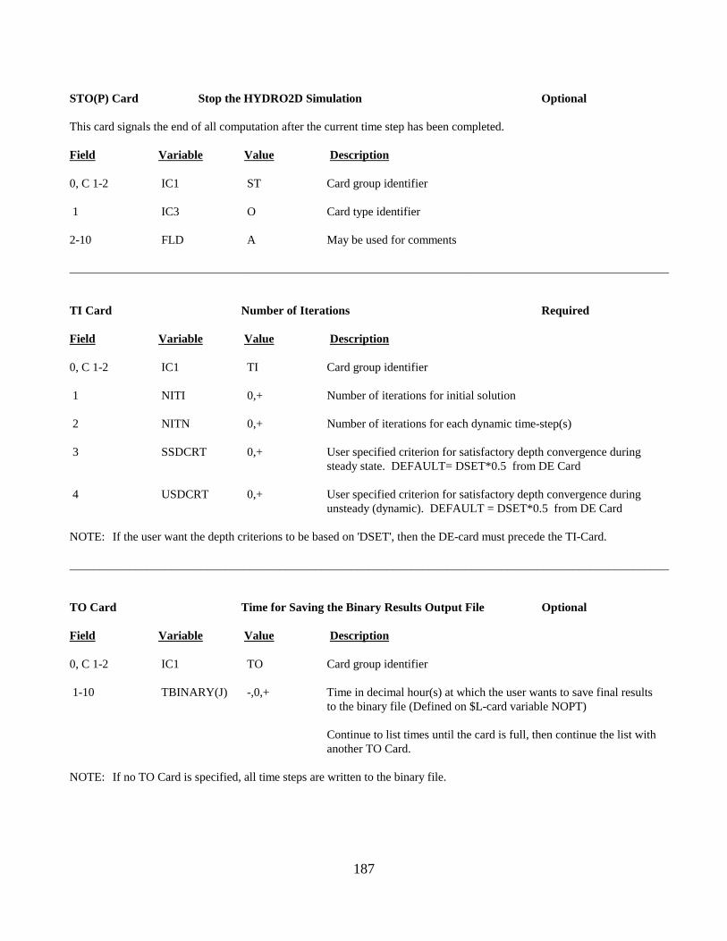
____________________________________________________________________________________________________
____________________________________________________________________________________________________
STO(P) Card Stop the HYDRO2D Simulation Optional
This card signals the end of all computation after the current time step has been completed.
Field Variable Value Description
0, C 1-2 IC1 ST Card group identifier
1 IC3 O Card type identifier
2-10 FLD A May be used for comments
TI Card Number of Iterations Required
Field Variable Value Description
0, C 1-2 IC1 TI Card group identifier
1 NITI 0,+ Number of iterations for initial solution
2 NITN 0,+ Number of iterations for each dynamic time-step(s)
3 SSDCRT 0,+ User specified criterion for satisfactory depth convergence during steady state. DEFAULT= DSET*0.5 from DE Card
4 USDCRT 0,+ User specified criterion for satisfactory depth convergence during unsteady (dynamic). DEFAULT = DSET*0.5 from DE Card
NOTE: If the user want the depth criterions to be based on 'DSET', then the DE-card must precede the TI-Card.
TO Card Time for Saving the Binary Results Output File Optional
Field Variable Value Description
0, C 1-2 IC1 TO Card group identifier
1-10 TBINARY(J) -,0,+ Time in decimal hour(s) at which the user wants to save final results to the binary file (Defined on $L-card variable NOPT)
Continue to list times until the card is full, then continue the list with another TO Card.
NOTE: If no TO Card is specified, all time steps are written to the binary file.
187
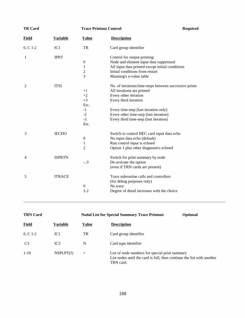
____________________________________________________________________________________________________
TR Card Trace Printout Control Required
Field Variable Value Description
0, C 1-2 IC1 TR Card group identifier
1 IPRT Control for output printing: 0 Node and element input data suppressed 1 All input data printed except initial conditions 2 Initial conditions from restart 3 Manning's n-value table
2 ITSI No. of iterations/time-steps between successive prints +1 All iterations are printed +2 Every other iteration +3 Every third iteration Etc. -1 Every time-step (last iteration only) -2 Every other time-step (last iteration) -3 Every third time-step (last iteration) Etc.
3 IECHO Switch to control HEC card input data echo 0 No input data echo (default) 1 Run control input is echoed 2 Option 1 plus other diagnostics echoed
4 ISPRTN Switch for print summary by node -, 0 De-activate the option
(even if TRN cards are present)
5 ITRACE Trace subroutine calls and controllers (for debug purposes only)
0 No trace 1-2 Degree of detail increases with the choice
TRN Card Nodal List for Special Summary Trace Printout Optional
Field Variable Value Description
0, C 1-2 IC1 TR Card group identifier
C3 IC3 N Card type identifier
NSPLPT(J) + List of node numbers for special print summary List nodes until the card is full, then continue the list with another TRN card.
188
1-10
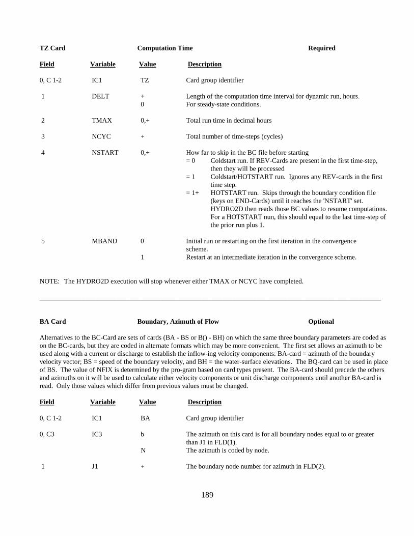
____________________________________________________________________________________________________
TZ Card Computation Time Required
Field Variable Value Description
0, C 1-2 IC1 TZ Card group identifier
1 DELT + Length of the computation time interval for dynamic run, hours. 0 For steady-state conditions.
2 TMAX 0,+ Total run time in decimal hours
3 NCYC + Total number of time-steps (cycles)
4 NSTART 0,+ How far to skip in the BC file before starting = 0 Coldstart run. If REV-Cards are present in the first time-step,
then they will be processed = 1 Coldstart/HOTSTART run. Ignores any REV-cards in the first
time step. = 1+ HOTSTART run. Skips through the boundary condition file
(keys on END-Cards) until it reaches the 'NSTART' set. HYDRO2D then reads those BC values to resume computations. For a HOTSTART nun, this should equal to the last time-step of the prior run plus 1.
5 MBAND 0 Initial run or restarting on the first iteration in the convergence scheme.
1 Restart at an intermediate iteration in the convergence scheme.
NOTE: The HYDRO2D execution will stop whenever either TMAX or NCYC have completed.
BA Card Boundary, Azimuth of Flow Optional
Alternatives to the BC-Card are sets of cards (BA - BS or B() - BH) on which the same three boundary parameters are coded as on the BC-cards, but they are coded in alternate formats which may be more convenient. The first set allows an azimuth to be used along with a current or discharge to establish the inflow-ing velocity components: BA-card = azimuth of the boundary velocity vector; BS = speed of the boundary velocity, and BH = the water-surface elevations. The BQ-card can be used in place of BS. The value of NFIX is determined by the pro-gram based on card types present. The BA-card should precede the others and azimuths on it will be used to calculate either velocity components or unit discharge components until another BA-card is read. Only those values which differ from previous values must be changed.
Field Variable Value Description
0, C 1-2 IC1 BA Card group identifier
0, C3 IC3 b The azimuth on this card is for all boundary nodes equal to or greater than J1 in FLD(1).
N The azimuth is coded by node.
1 J1 + The boundary node number for azimuth in FLD(2).
189
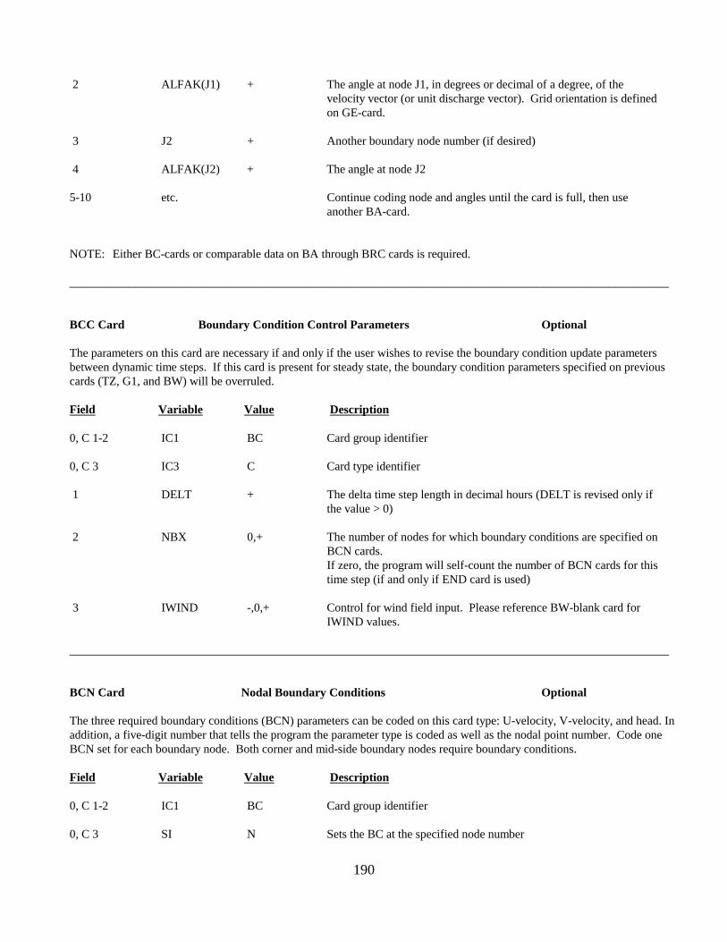
____________________________________________________________________________________________________
____________________________________________________________________________________________________
2 ALFAK(J1) + The angle at node J1, in degrees or decimal of a degree, of the velocity vector (or unit discharge vector). Grid orientation is defined on GE-card.
3 J2 + Another boundary node number (if desired)
4 ALFAK(J2) + The angle at node J2
5-10 etc. Continue coding node and angles until the card is full, then use another BA-card.
NOTE: Either BC-cards or comparable data on BA through BRC cards is required.
BCC Card Boundary Condition Control Parameters Optional
The parameters on this card are necessary if and only if the user wishes to revise the boundary condition update parameters between dynamic time steps. If this card is present for steady state, the boundary condition parameters specified on previous cards (TZ, G1, and BW) will be overruled.
Field Variable Value Description
0, C 1-2 IC1 BC Card group identifier
0, C 3 IC3 C Card type identifier
1 DELT + The delta time step length in decimal hours (DELT is revised only if the value > 0)
2 NBX 0,+ The number of nodes for which boundary conditions are specified on BCN cards. If zero, the program will self-count the number of BCN cards for this time step (if and only if END card is used)
3 IWIND -,0,+ Control for wind field input. Please reference BW-blank card for IWIND values.
BCN Card Nodal Boundary Conditions Optional
The three required boundary conditions (BCN) parameters can be coded on this card type: U-velocity, V-velocity, and head. In addition, a five-digit number that tells the program the parameter type is coded as well as the nodal point number. Code one BCN set for each boundary node. Both corner and mid-side boundary nodes require boundary conditions.
Field Variable Value Description
0, C 1-2 IC1 BC Card group identifier
0, C 3 SI N Sets the BC at the specified node number
190
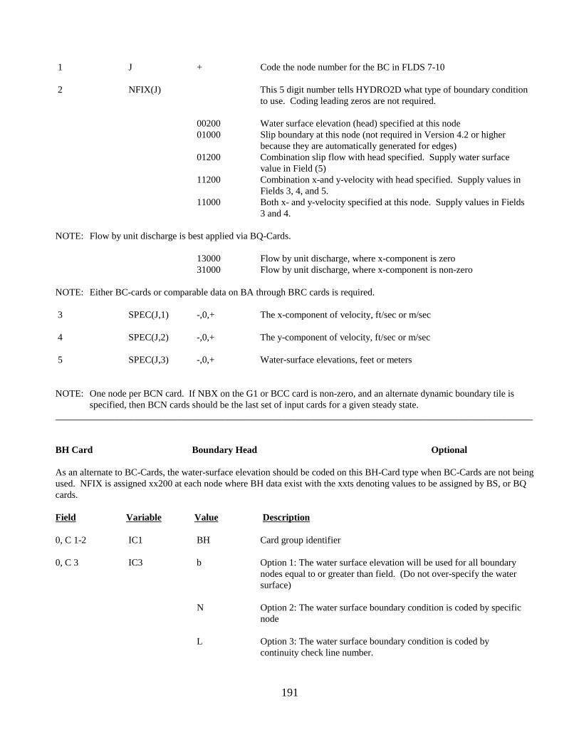
____________________________________________________________________________________________________
1 J + Code the node number for the BC in FLDS 7-10
2 NFIX(J) This 5 digit number tells HYDRO2D what type of boundary condition to use. Coding leading zeros are not required.
00200 Water surface elevation (head) specified at this node 01000 Slip boundary at this node (not required in Version 4.2 or higher
because they are automatically generated for edges) 01200 Combination slip flow with head specified. Supply water surface
value in Field (5) 11200 Combination x-and y-velocity with head specified. Supply values in
Fields 3, 4, and 5. 11000 Both x- and y-velocity specified at this node. Supply values in Fields
3 and 4.
NOTE: Flow by unit discharge is best applied via BQ-Cards.
13000 Flow by unit discharge, where x-component is zero 31000 Flow by unit discharge, where x-component is non-zero
NOTE: Either BC-cards or comparable data on BA through BRC cards is required.
3 SPEC(J,1) -,0,+ The x-component of velocity, ft/sec or m/sec
4 SPEC(J,2) -,0,+ The y-component of velocity, ft/sec or m/sec
5 SPEC(J,3) -,0,+ Water-surface elevations, feet or meters
NOTE: One node per BCN card. If NBX on the G1 or BCC card is non-zero, and an alternate dynamic boundary tile is specified, then BCN cards should be the last set of input cards for a given steady state.
BH Card Boundary Head Optional
As an alternate to BC-Cards, the water-surface elevation should be coded on this BH-Card type when BC-Cards are not being used. NFIX is assigned xx200 at each node where BH data exist with the xxts denoting values to be assigned by BS, or BQ cards.
Field Variable Value Description
0, C 1-2 IC1 BH Card group identifier
0, C 3 IC3 b Option 1: The water surface elevation will be used for all boundary nodes equal to or greater than field. (Do not over-specify the water surface)
N Option 2: The water surface boundary condition is coded by specific node
L Option 3: The water surface boundary condition is coded by continuity check line number.
191
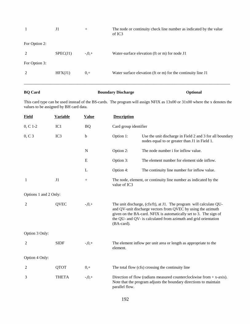
____________________________________________________________________________________________________
1 J1 + The node or continuity check line number as indicated by the value of IC3
For Option 2:
2 SPEC(J1) -,0,+ Water-surface elevation (ft or m) for node J1
For Option 3:
2 HFX(J1) 0,+ Water surface elevation (ft or m) for the continuity line J1
BQ Card Boundary Discharge Optional
This card type can be used instead of the BS-cards. The program will assign NFIX as 13x00 or 31x00 where the x denotes the values to be assigned by BH card data.
Field Variable Value Description
0, C 1-2 IC1 BQ Card group identifier
0, C 3 IC3 b Option 1: Use the unit discharge in Field 2 and 3 for all boundary nodes equal to or greater than J1 in Field 1.
N Option 2: The node number i for inflow value.
E Option 3: The element number for element side inflow.
L Option 4: The continuity line number for inflow value.
1 J1 + The node, element, or continuity line number as indicated by the value of IC3
Options 1 and 2 Only:
2 QVEC -,0,+ The unit discharge, (cfs/ft), at J1. The program will calculate QU-and QV-unit discharge vectors from QVEC by using the azimuth given on the BA-card. NFIX is automatically set to 3. The sign of the QU- and QV- is calculated from azimuth and grid orientation (BA-card).
Option 3 Only:
2 SIDF -,0,+ The element inflow per unit area or length as appropriate to the element.
Option 4 Only:
2 QTOT 0,+ The total flow (cfs) crossing the continuity line
3 THETA -,0,+ Direction of flow (radians measured counterclockwise from + x-axis). Note that the program adjusts the boundary directions to maintain parallel flow.
192
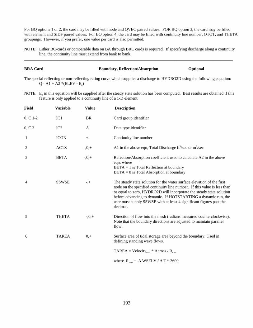
____________________________________________________________________________________________________
For BQ options 1 or 2, the card may be filled with node and QVEC paired values. FOR BQ option 3, the card may be filled with element and SIDF paired values. For BO option 4, the card may be filled with continuity line number, OTOT, and THETA groupings. However, if you prefer, one value per card is also permitted.
NOTE: Either BC-cards or comparable data on BA through BRC cards is required. If specifying discharge along a continuity line, the continuity line must extend from bank to bank.
BRA Card Boundary, Reflection/Absorption Optional
The special reflecting or non-reflecting rating curve which supplies a discharge to HYDRO2D using the following equation: Q= A1 + A2 *(ELEV - Eo)
NOTE: Eo in this equation will be supplied after the steady state solution has been computed. Best results are obtained if this feature is only applied to a continuity line of a 1-D element.
Field Variable Value Description
0, C 1-2 IC1 BR Card group identifier
0, C 3 IC3 A Data type identifier
1 ICON + Continuity line number
2 AC1X -,0,+ A1 in the above eqn, Total Discharge ft3/sec or m3/sec
3 BETA -,0,+ Refection/Absorption coefficient used to calculate A2 in the above eqn, where BETA = 1 is Total Reflection at boundary BETA = 0 is Total Absorption at boundary
4 SSWSE -,+ The steady state solution for the water surface elevation of the first node on the specified continuity line number. If this value is less than or equal to zero, HYDRO2D will incorporate the steady state solution before advancing to dynamic. If HOTSTARTING a dynamic run, the user must supply SSWSE with at least 4 significant figures past the decimal.
5 THETA -,0,+ Direction of flow into the mesh (radians measured counterclockwise). Note that the boundary directions are adjusted to maintain parallel flow.
6 TAREA 0,+ Surface area of tidal storage area beyond the boundary. Used in defining standing wave flows.
TAREA = Velocitymax * Across / Rmax
where Rmax = ) WSELV / ) T * 3600
193
____________________________________________________________________________________________________
____________________________________________________________________________________________________
BRC Card Boundary, Rating Curve Optional
The rating curve supplies a discharge to HYDRO2D using the following equation: Q = A1 + A2*(ELEV-E0)**C
Field Variable Value Description
0, C 1-2 IC1 BR Card group identifier
0, C 3 IC3 C Data type identifier
1 JCR + Continuity line number
2 AC1X -,0,+ A1 in the above equation
3 AC2X -,0,+ A2 in the above equation
4 AC3X -,0,+ E0 in the above equation
5 AC4X -,0,+ C in the above equation
6 THETA -,0,+ Direction of flow (radians measured counterclockwise from positive x -axis). Note that the boundary directions are adjusted to maintain
parallel flow.
BS Card Boundary Current Speed Optional
The magnitude of the velocity vector is coded on this card type. The input data program will convert BS data to U- and V-velocity components using the azimuth on the preceding BA-card. Sign of the component is calculated from its azimuth and the specified grid orientation (G1-Card). NFIX is assigned a value of 11x00 at each node having a BS value where the x denotes a value to be assigned by presence of BH-card data.
Field Variable Value Description
0, C 1-2 IC1 BR
0, C 3 ISI b
N
1 J1 +
2 WEC1 0,+
3 J2 +
4 VVEC2 0,+
Card group identifier
Use the boundary condition (BC) in Field 1 for all boundary nodes equal to or greater than Field 3.
The node number is coded for each BC value on this card
Node number
Current speed in fps at node J1. Sign will be determined from the azimuth of the vector
Next node
Current speed at node J2, ft/sec or m/sec
194
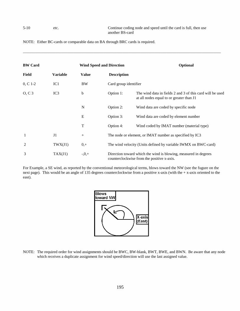
____________________________________________________________________________________________________
5-10 etc. Continue coding node and speed until the card is full, then use another BS-card
NOTE: Either BC-cards or comparable data on BA through BRC cards is required.
BW Card Wind Speed and Direction Optional
Field Variable Value Description
0, C 1-2 IC1 BW Card group identifier
O, C 3 IC3 b Option 1: The wind data in fields 2 and 3 of this card will be used at all nodes equal to or greater than J1
N Option 2: Wind data are coded by specific node
E Option 3: Wind data are coded by element number
T Option 4: Wind coded by IMAT number (material type)
1 J1 + The node or element, or IMAT number as specified by IC3
2 TWX(J1) 0,+ The wind velocity (Units defined by variable IWMX on BWC-card)
3 TAX(J1) -,0,+ Direction toward which the wind is blowing, measured in degrees counterclockwise from the positive x-axis.
For Example, a SE wind, as reported by the conventional meteorological terms, blows toward the NW (see the fugure on the next page). This would be an angle of 135 degrees counterclockwise from a positive x-axis (with the + x-axis oriented to the east).
NOTE: The required order for wind assignments should be BWC, BW-blank, BWT, BWE, and BWN. Be aware that any node which receives a duplicate assignment for wind speed/direction will use the last assigned value.
195
BWC Card Boundary, Wind Control Formulation Optional
The BWC card followed by a BW type card for wind speed and direction is required if a wind field is to be applied in HYDRO2D.
Field Variable Value Description
0, C 1-2 IC1 BW Card group identifier
1 IWIND -,0,+ Control for wind field input IWIND = 0 no wind input IWIND < 0 wind field specified for all nodes using one line of input (BW-blank card) IWIND > 0 wind field specified at each node.
Type of Wind Formula
ABS(IWIND) = 1 Original formulation ABS(IWIND) = 2 Van Dorn Formula with user supplied
coefficients ABS(IWIND) = 3 Wu Formula with user supplied coefficients ABS(IWIND) = 4 Safaie Formula with user supplied coefficients ABS(IWIND) = 5 Ekman Formula with default coefficients ABS(IWIND) = 6 Generic Formula with user supplied
coefficients ABS(IWIND) = 7 Van Dorn Formula default coefficients ABS(IWIND) = 8 Wu Formula with default coefficients
2 IWMX 0,1 Flag to identify the units of the wind speed (recorded at height=10 m). IWMX = 0 for miles/hour IWMX = 1 for meters/second
Specify Field 3-6 as Needed
3 WC1 Fields 3-6 will be the necessary coefficients required for the wind formulation as defined by the variable IWIND above.
4 WC2
5 WC3
6 WC4
------------- Special Instruction ------------------
If ABS(IWIND) = 2 Van Dorn WC1 = 10 meters, Anemometer height WC2 = Smooth water wind stress coefficient WC3 = Rough water wind stress coefficient WC4 = Critical wind velocity for wave formulation (m/s)
If ABS(IWIND) = 3 WU Formula
196
____________________________________________________________________________________________________
WC1 = 10 meters, Anemometer heightWC2 = Wind stress coefficientWC3 = Air Density
If WC3 > 0.0 units should be g/cm3,If WC3 > 0.0 default of 0.001226 g/cm3 used(Dry air at 1 atm pressure and 15oC)
WC4 = unused
If ABS(IWIND) = 4 Safaie Formula WC1 = Charnock's constant
If WC1 < 0.0 default of 0.0332 usedWC2 = Dynamic roughness in cm (no default)WC3 = Acceleration due to gravity (affects wind formula only)
If WC3 > 0.0 units should be cm/s2
If WC3 < 0.0 default value of 979.965 cm/s2 usedWC4 = Air density
If WC4 > 0.0 units should be g/cm3
If WC4 < 0.0 default value of 0.001226 g/cm3 used(Dry air at 1 atm pressure and 15oC)
If ABS(IWIND) = 6 Generic Formula WC1 = 10 meter, Anemometer height WC2 = Wind stress coefficient (no default) WC3 = Empirical exponent (no default) WC4 = Air density
If WC4 > 0.0 units should be g/cm3
If WC4 < 0.0 default value of .001226 g/cm3 used(Dry air at 1 atm pressure and 15oC)
If ABS(IWIND) = 1, 5, 7 or 8 then WC1, WC2, WC3, and WC4 should all be zero
BWS Card Boundary, Wind Storm Optional (see Figure C.2 for explanation)
Field Variable Value Description
0, C 1-2 IC1 BW Card group identifier
0, C 3 IC3 S Card type identifier
1 ISTYPE + Storm reference point (3 = Center)
2 NREF + Reference node for storm track
3 TREF + Reference HYDRO2D simulation time for storm to arrive at node'NREF'
4 SSPD + Storm speed, mph
5 WNDMAX + Maximum wind speed, mph
197

6 WINDMIN + Minimum or base wind level, mph
7 THETAS + Direction of storm track, degrees counterclockwise from positive x-axis toward which the storm is moving
8 THETAT + Orientation of from (0,180 deg) relative to x-axis in degrees counterclockwise
9 BETAL + Standard deviation of spatial distribution function in the direction of the storm's movement
10 BETAT + Standard deviation of spatial distribution function in the direction transverse to storm path
11 DECAY + Exponential temporal decay for windspeed (hr-1)
NOTE: Each BWS-Card creates a storm, you may run multiple storms (presently dimensioned to 2)
198
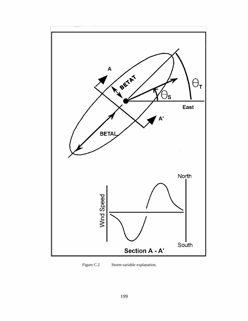
Figure C.2 Storm variable explanation.
199