Embed Size (px)
DESCRIPTION
FEA
Citation preview

Finite Element Analysisof
2-Dimensional Problems
Jayadeep U. B.
M.E.D., NIT Calicut
Ref.: Finite Elements and Approximation, Zienkiewicz, O. C., and Morgan, K., John Wiley & Sons.

2
Department of Mechanical Engineering, National Institute of Technology Calicut
Introduction
The heat transfer problem in a 2-D plate can be analyzed as a 2-D problem (assuming temperature gradient to be zero in the thickness direction).
Examples of 2-D Problems – Heat Transfer Problem:
Even if the heat transfer is not 2D, e.g., if convective losses are taking place from this surface of plate, we may be able to formulate the problem as 2D.
Dirichlet or
(Essential) B.C.
on T Neumann or (Natural) B.C.
on qq k qn
Convective B.C. on h
q k hn
Lecture - 01
3
Department of Mechanical Engineering, National Institute of Technology Calicut
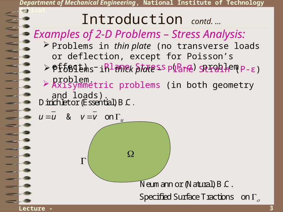
Introduction contd. …
Problems in thin plate (no transverse loads or deflection, except for Poisson’s effect) – Plane Stress (P-σ) problem.
Examples of 2-D Problems – Stress Analysis:
Dirichlet or (Essential) B.C.
& on uu u v v
Problems in thick plate – Plane Strain (P-ε) problem.
Axisymmetric problems (in both geometry and loads).
Neumann or (Natural) B.C.
Specified Surface Tractions on Lecture - 01

4
Department of Mechanical Engineering, National Institute of Technology Calicut
Finite Elements for 2D A fundamental idea in FEM is to discretize the complicated
domain into simple shapes, over which the integrations can be easily performed.
In 2D, the normally used shapes are triangles and rectangles – other shapes are not having any special advantage.
The vertices of the triangles and the rectangles can be used as the nodes, at which the finite elements are connected with each other.
In case of higher order elements we can have nodes on the edges as well as interior to the domain.
The simple forms of shape functions, which will be discussed in subsequent sections will be applicable only for C0 continuous problems (Only first order derivatives are occurring in the weak form).
Lecture - 01

5
Department of Mechanical Engineering, National Institute of Technology Calicut
The Linear Triangle Element
The simplest element type possible in 2D is the linear triangle.
Triangular element has the added advantage that any complicated shape can be better approximated as compared to rectangles.
A combination of triangles and rectangles can improve the approximation (triangular elements near the boundary), but there are better methods available!!!
Lecture - 01

6
Department of Mechanical Engineering, National Institute of Technology Calicut
We can use the same ideas as in 1D to derive the shape functions for 2D triangular elements.
Shape Functions for Linear Triangle:The Linear Triangle Element cont. …
Any linear variation over a planar triangular element (assumed to be in x-y plane) as a combination of three linear shape functions.
Let node be at , , be at , & be at , .
1 at ( , )
The shape function, 0 at ( , )
0 at ( , )
Assume,
1, 0 & 0
i i j j k k
i i
i j j
k k
i
i i j j k k
i x y j x y k x y
x y
N x y
x y
N a bx cy
a bx cy a bx cy a bx cy
Lecture - 01

7
Department of Mechanical Engineering, National Institute of Technology Calicut
Shape Functions for Linear Triangle contd.:The Linear Triangle Element cont. …
Writing in Matrix form:
1 1
1 0
1 0
1 1 1 1 1
det 0 det 1 0 det 1 0
0 1 0 1 0, &
1 1 1
det 1 det 1 det
1 1
i i
j j
k k
i i i i
j j j j
k k k k
i i i i
j j j j
k k k k
x y a
x y b
x y c
x y y x
x y y x
x y y xa b c
x y x y x
x y x y
x y x y
1
1
i i
j j
k k
y
x y
x y
Lecture - 01
8
Department of Mechanical Engineering, National Institute of Technology Calicut
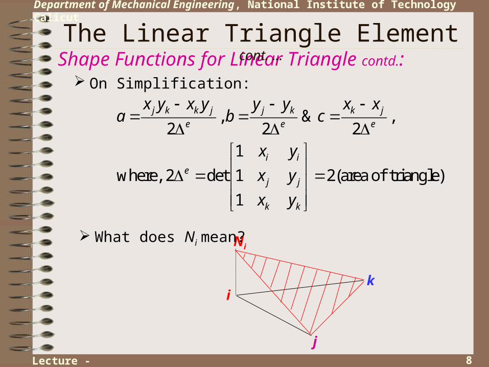
Shape Functions for Linear Triangle contd.:The Linear Triangle Element cont. …
On Simplification:
, & ,2 2 2
1
where, 2 det 1 2(area of triangle)
1
j k k j j k k j
e e e
i ie
j j
k k
x y x y y y x xa b c
x y
x y
x y
ik
j
Ni What does Ni mean?
Lecture - 01

9
Department of Mechanical Engineering, National Institute of Technology Calicut
Shape Functions for Linear Triangle contd.:The Linear Triangle Element cont. …
Further geometric meaning of Ni: The area coordinates
i
k
j
Ni
Nj
Nk
( , , )l l x y z
area of area of area of , &
area of area of area of i j k
jkl ilk ijlN N N
ijk ijk ijk
Lecture - 01
10
Department of Mechanical Engineering, National Institute of Technology Calicut
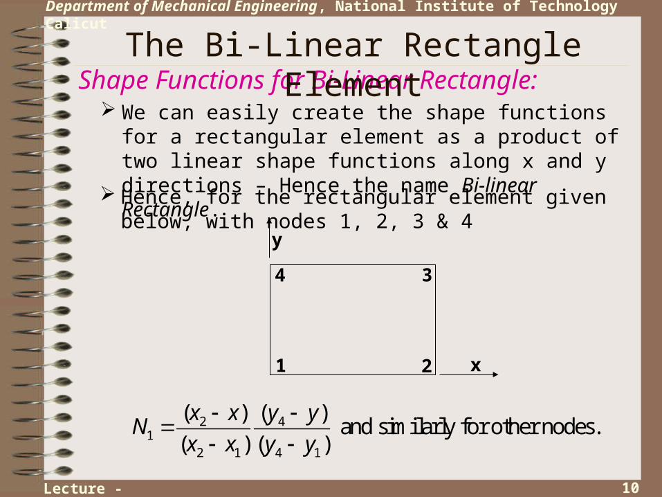
We can easily create the shape functions for a rectangular element as a product of two linear shape functions along x and y directions – Hence the name Bi-linear Rectangle.
Shape Functions for Bi-Linear Rectangle:The Bi-Linear Rectangle Element
2 41
2 1 4 1
( ) ( ) and similarly for other nodes.
( ) ( )
x x y yN
x x y y
Hence, for the rectangular element given below, with nodes 1, 2, 3 & 4
1 2
34
x
y
Lecture - 01
11
Department of Mechanical Engineering, National Institute of Technology Calicut
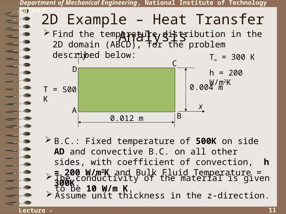
Find the temperature distribution in the 2D domain (ABCD), for the problem described below:
2D Example – Heat Transfer Analysis
B.C.: Fixed temperature of 500K on side AD and convective B.C. on all other sides, with coefficient of convection, h = 200 W/m2K and Bulk Fluid Temperature = 300K.
The conductivity of the material is given to be 10 W/m K.
T = 500 K
0.012 m
0.004 m
AB
CD
T∞ = 300 K
h = 200 W/m2K
x
y
Assume unit thickness in the z-direction.
Lecture - 02

12
Department of Mechanical Engineering, National Institute of Technology Calicut
Governing D.E.:
2D Heat Transfer Analysis contd. …
B.C.:
2 2
2 2
0
Since, is constant and 0,
0 on
k k Qx x y y
k Q
ABCDx y
500 on
on , ,ˆ
10 200 300 on , 10 200 300 on
& 10 200 300 on
h
AD
k h AB BC CD
AB BCy x
CDy
n
Lecture - 02

13
Department of Mechanical Engineering, National Institute of Technology Calicut
FE Mesh using linear triangle elements:
2D Heat Transfer Analysis contd. …
Approximation:1
2
12
12
34
56
78
910
1112
3 4
5 6 7 8
910 11
x
y
3
1
ˆ on (any element)ej j
j
N
Weighted Residual Formulation is used.
Lecture - 02

14
Department of Mechanical Engineering, National Institute of Technology Calicut
2D Heat Transfer Analysis contd. …
W.R. Statement (Strong Form):
2 2
2 2
2
ˆ ˆ ˆˆ( ) 0
ˆ
ˆˆ ˆ( ) ( ) 0
ˆ
h
h
i i
i i
hW d W d
x y k
hW d W d
k
n
n
Note: Strong form of W.R. statement can not be used since the second derivative of the shape functions (linear polynomials) are identically equal to zero. Only the boundary residuals will have non-zero terms.
The Weak Form needs to be formulated.
Since the essential B.C. (specified temperature) can be enforced exactly, no residual is assumed on side AD.
Lecture - 02
15
Department of Mechanical Engineering, National Institute of Technology Calicut
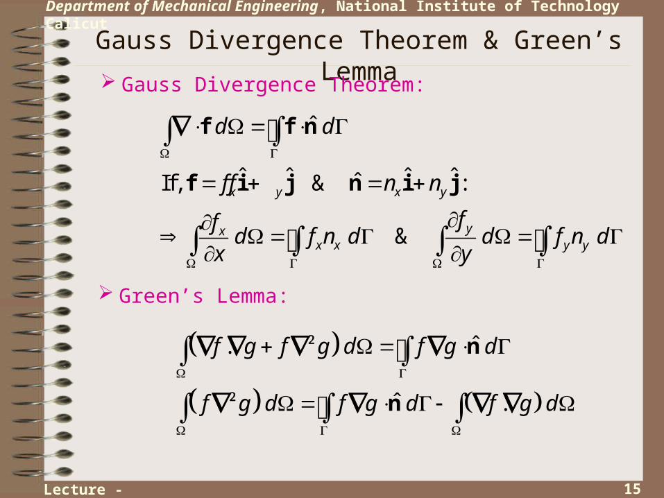
Gauss Divergence Theorem & Green’s Lemma
Gauss Divergence Theorem:
ˆ
ˆ ˆ ˆ ˆˆIf, & :
&
x y x y
yxx x y y
d d
f f n n
ffd f n d d f n d
x y
f f n
f i j n i j
Green’s Lemma:
ˆ.
ˆ .
f g f g d f g d
f g d f g d f g d
n
n
Lecture - 02

16
Department of Mechanical Engineering, National Institute of Technology Calicut
Applying Green’s Lemma to the Strong form:
ˆˆ ˆ ˆˆ. ( ) 0
ˆh
i i i
hW d W d W d
k
nn
We have:
ˆ
ˆ ˆ. ,ˆ
and let ,
h
i i iW N W
nn
2D Heat Transfer Analysis contd. …
Using the Galerkin formulation & simplifying:
ˆˆ ˆ( ) 0
ˆh
i i i
hN d N d N d
k
n
Lecture - 02

17
Department of Mechanical Engineering, National Institute of Technology Calicut
Substituting the approximation, we have the Weak Form:
2D Heat Transfer Analysis contd. …
ˆ
ˆ
h
h
j jj
i j j ij
i i
h N
N N d N dk
hN d N d
k
n
Re-arranging the terms & Simplifying:
ˆ
ˆ
h
h
j ji ij i j
j
i i
N NN N hd d N N d
x x y y k
hN d N d
k
nLecture - 02
18
Department of Mechanical Engineering, National Institute of Technology Calicut
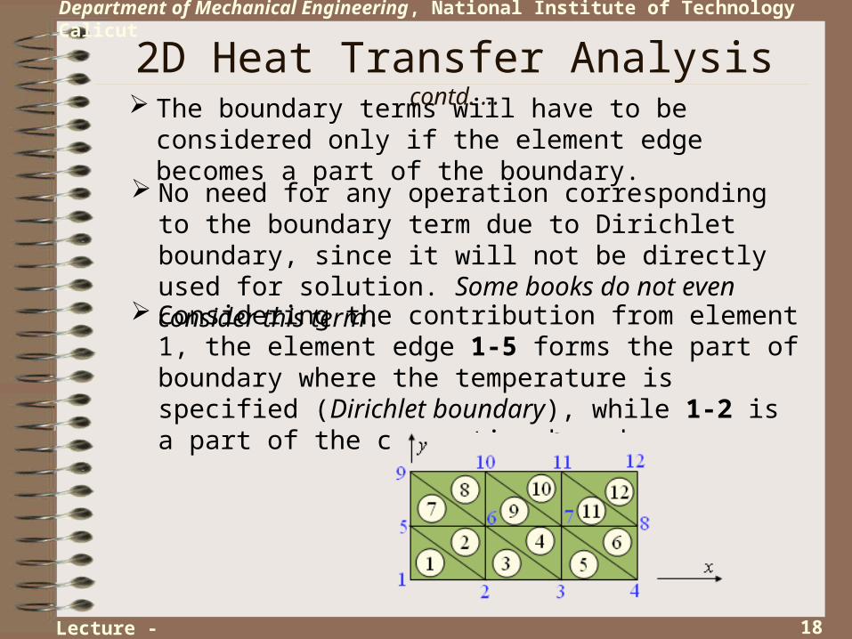
The boundary terms will have to be considered only if the element edge becomes a part of the boundary.
2D Heat Transfer Analysis contd. …
Considering the contribution from element 1, the element edge 1-5 forms the part of boundary where the temperature is specified (Dirichlet boundary), while 1-2 is a part of the convective boundary.
No need for any operation corresponding to the boundary term due to Dirichlet boundary, since it will not be directly used for solution. Some books do not even consider this term.
Lecture - 02

19
Department of Mechanical Engineering, National Institute of Technology Calicut
Consider the shape functions for element 1:
2D Heat Transfer Analysis contd. …
, &
, where 1, 2 & 5.
i i i i j j j j
k k k k
N a b x c y N a b x c y
N a b x c y i j k
6
0.004 0.0021
2 2 4 10
250 & 5002 2
1 250 500
j k k ji e
j k k ji ie e
i
x y x ya
y y x xb c
N x y
We get the shape function Ni:
250 & 500j kN x N y
Similarly we get the other shape functions:
Lecture - 02

20
Department of Mechanical Engineering, National Institute of Technology Calicut
2D Heat Transfer Analysis contd. …
Stiffness Matrix Components for element 1:
1 1
1 1
2221
2 22 2 2 2 1
ij
ij ij
i iii i
i i i i i i
N N hK d d N d
x y k
h hb d c d N d b c N d
k k
Ni
(Ni)2
i j
12
2 1 0.0040.00133,
3 3
where is the length of side
i ij
ij ij
N d S
S
Area of element 1
Evaluation of the boundary term:
Lecture - 02

21
Department of Mechanical Engineering, National Institute of Technology Calicut
2D Heat Transfer Analysis contd. …
Substituting the values:
21 2 2 1
2 2 6250 500 4 10 20 0.00133 1.277
ij
ii i i i
hK b c N d
k
Ni
i j
1 200 300
10 2
6000 0.002 12ij
iji i
Shf N d
k
Right-side vector component:
Lecture - 02

22
Department of Mechanical Engineering, National Institute of Technology Calicut
2D Heat Transfer Analysis contd. …
Second Stiffness Matrix component:
1 1
1
1
1
ij
ij
ij
j ji iij i j
i j i j i j
i j i j i j
N NN N hK d d N N d
x x y y k
hb b c c d N N d
k
hb b c c N N d
k
12
1 0.0040.000667,
6 6
where is the length of side
i j ij
ij ij
N N d S
S
Evaluation of Boundary term:
Ni
i j
Nj
Ni Nj
Lecture - 02

23
Department of Mechanical Engineering, National Institute of Technology Calicut
2D Heat Transfer Analysis contd. …
Substituting the values:
1 1
2 6250 4 10 20 0.000667 0.237
ij
ij i j i j i j
hK b b c c N N d
k
Third stiffness matrix component:
1 1
1
1
1 2 6500 4 10 1
ij
i k i kik i k
i k i k i k i k
N N N N hK d d N N d
x x y y k
b b c c d b b c c
= 0
Lecture - 02
24
Department of Mechanical Engineering, National Institute of Technology Calicut
2D Heat Transfer Analysis contd. …
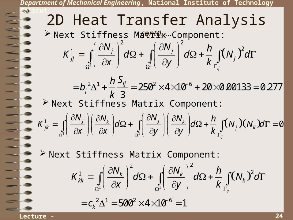
Next Stiffness Matrix Component:
1 1
2 221
2 1 2 6250 4 10 20 0.00133 0.2773
ij
j jjj j
ijj
N N hK d d N d
x y k
Shb
k
1 1
1 0ij
j jk kjk j k
N NN N hK d d N N d
x x y y k
Next Stiffness Matrix Component:
Next Stiffness Matrix Component:
1 1
2221
2 1 2 6500 4 10 1
ij
k kkk k
k
N N hK d d N d
x y k
c
Lecture - 02

25
Department of Mechanical Engineering, National Institute of Technology Calicut
2D Heat Transfer Analysis contd. …
1
1
200 300
10 2
6000 0.002 12
0
ij
ij
ijj j
k k
Shf N d
k
hf N d
k
Right-side vector components:
Writing in the matrix form, the elemental system:
1 1
1.277 0.237 1 12
0.237 0.277 0 & 12
1 0 1 0
K f
Lecture - 02

26
Department of Mechanical Engineering, National Institute of Technology Calicut
2D Heat Transfer Analysis contd. …
0 0 0 0 0 0 0 0 0
0 0 0 0 0 0 0 0 0
0 0 0 0 0 0 0 0 0 0 0 0
0 0 0 0 0 0 0 0 0 0 0 0
0 0 0 0 0 0 0 0 0
0 0 0 0 0 0 0 0 0 0 0 0
0 0 0 0 0 0 0 0 0 0 0 0
0 0 0 0 0 0 0 0 0 0 0 0
0 0 0 0 0 0 0 0 0 0 0 0
0 0 0 0 0 0 0 0 0 0 0 0
0 0 0 0 0 0 0 0 0 0 0 0
0 0 0 0 0 0 0 0 0 0 0 0
K
0
0 1
1.277 -0.237 -1
-0.237 0.277
-1
12
12
0
0
0
0&
0
0
0
0
0
0
f
Assembly into the global system (Contribution from element 1 only is calculated):
Lecture - 03

27
Department of Mechanical Engineering, National Institute of Technology Calicut
Contribution from element 2:
2D Heat Transfer Analysis contd. …
, &
, where 2, 6 & 5.
i i i i j j j j
k k k k
N a b x c y N a b x c y
N a b x c y i j k
The nodal coordinates using the local coordinate system:
2 (0,0), 6 (0,0.002) & 5 ( 0.004,0.002)i j k
It is convenient to define the local coordinate system – Translate the coordinate system to coincide the origin with node 2:
1 500 , 250 500 & 250
1, 0 & 500
0, 250 & 500
0, 250 & 0
i j k
i i i
j j j
k k k
N y N x y N x
a b c
a b c
a b c
The shape functions:
Lecture - 03

28
Department of Mechanical Engineering, National Institute of Technology Calicut
2D Heat Transfer Analysis contd. …
Stiffness Matrix Components for element 2:
2 2
2 2
222
2 2 2 2 2
i iii
i i i i
N NK d d
x y
b d c d b c
2 2 2 2 2 2 60 500 4 10 1ii i iK b c
Note: There is no boundary term, since the element 2 does not share any convective boundary.
Substituting the values:
Lecture - 03

29
Department of Mechanical Engineering, National Institute of Technology Calicut
2D Heat Transfer Analysis contd. …
Second Stiffness Matrix component:
2 2
2
2
2
60 500 500 4 10 1
j ji iij
i j i j i j i j
N NN NK d d
x x y y
b b c c d b b c c
Third stiffness matrix component:
2 2
2
2
0
i k i kik
i k i k
N N N NK d d
x x y y
b b c c d
Lecture - 03

30
Department of Mechanical Engineering, National Institute of Technology Calicut
2D Heat Transfer Analysis contd. …
Next Stiffness Matrix Component:
2 2
2 2
2
2 2 2 2 2 6( ) 250 500 4 10 1.25
j jjj
j j
N NK d d
x y
b c
2 2
2
2 2 6250 4 10 0.25
j jk kjk
j k j k
N NN NK d d
x x y y
b b c c
Next Stiffness Matrix Component:
Next Stiffness Matrix Component:
2 2
222
2 2 2 6250 4 10 0.25
k kkk
k
N NK d d
x y
b
Lecture - 03

31
Department of Mechanical Engineering, National Institute of Technology Calicut
2D Heat Transfer Analysis contd. …
Right-side vector components are all zero, since there is no convective boundary associated with element 2:
Writing in the matrix form, the elemental system:
2 2
1 1 0 0
1 1.25 0.25 & 0
0 0.25 0.25 0
K f
Lecture - 03

32
Department of Mechanical Engineering, National Institute of Technology Calicut
2D Heat Transfer Analysis contd. …
1.277 0.237 0 0 1 0 0 0 0 0 0 0
0.237 0 0 0 0 0 0 0 0
0 0 0 0 0 0 0 0 0 0 0 0
0 0 0 0 0 0 0 0 0 0 0 0
1 0 0 0 0 0 0 0 0
0 0 0 0 0 0 0 0 0
0 0 0 0 0 0 0 0 0 0 0 0
0 0 0 0 0 0 0 0 0 0 0 0
0 0 0 0 0 0 0 0 0 0 0 0
0 0 0 0 0 0 0 0 0 0 0 0
0 0 0 0 0 0 0 0 0 0 0 0
0 0 0 0 0 0 0 0 0 0 0 0
K
0
0
1.277 -1
1.25 -0.25
-1 -0.25 1.25
Adding the contribution from element 2 to the global stiffness matrix:
Lecture - 03
33
Department of Mechanical Engineering, National Institute of Technology Calicut
2D Heat Transfer Analysis contd. …
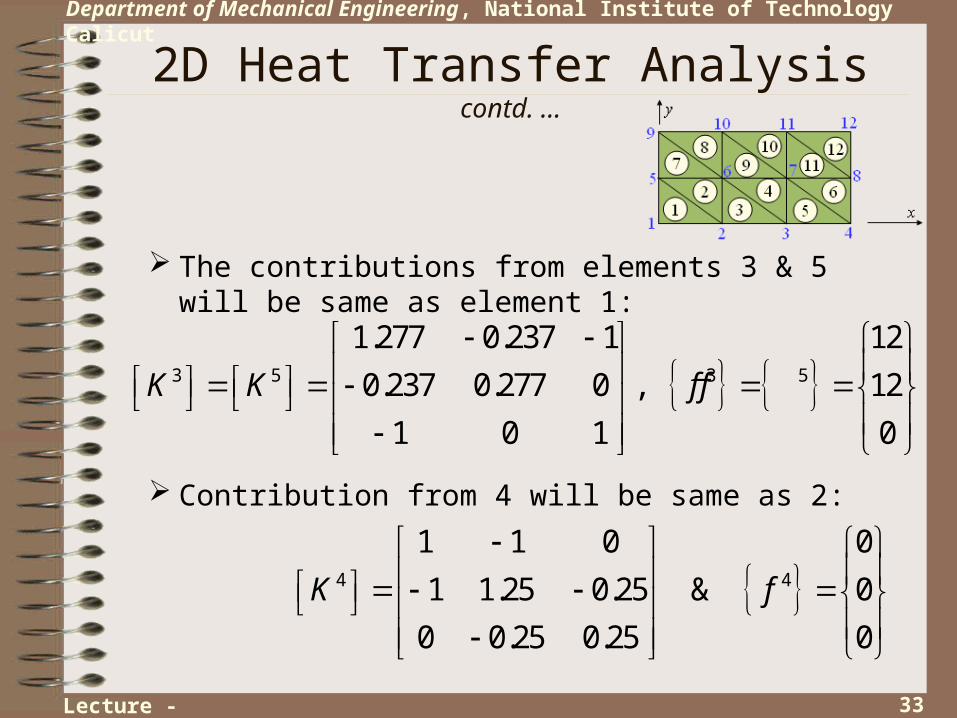
The contributions from elements 3 & 5 will be same as element 1:
3 5 3 5
1.277 0.237 1 12
0.237 0.277 0 , 12
1 0 1 0
K K f f
Contribution from 4 will be same as 2:
4 4
1 1 0 0
1 1.25 0.25 & 0
0 0.25 0.25 0
K f
Lecture - 03
34
Department of Mechanical Engineering, National Institute of Technology Calicut
2D Heat Transfer Analysis contd. …
1.277 0.237 0 0 1 0 0 0 0 0 0 0
0.237 0 0 0 0 0 0 0 0
0 0 0 0 0 0 0
0 0 0 0 0 0 0 0 0
1 0 0 0 1.25 -0.25 0 0 0 0 0 0
0 0 -0.25 0 0 0 0 0
0 0 0 0 0 0 0 0
0 0 0 0 0 0 0 0 0 0 0 0
0 0 0 0 0 0 0 0 0 0 0 0
0 0 0 0 0 0 0 0 0 0 0 0
0 0 0
0
0
0
0
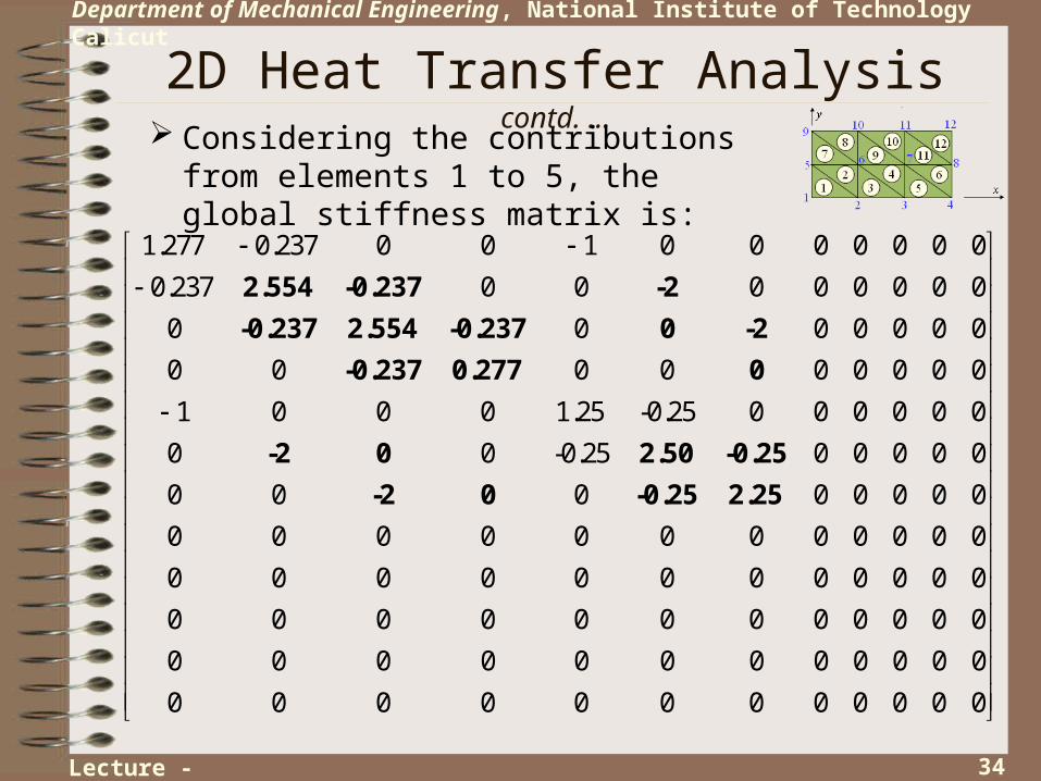
2.554 -0.237 -2
-0.237 2.554 -0.237 -2
-0.237 0.277
-2 2.50 -0.25
-2 -0.25 2.25
0 0 0 0 0 0 0 0 0
0 0 0 0 0 0 0 0 0 0 0 0
Considering the contributions from elements 1 to 5, the global stiffness matrix is:
Lecture - 03
35
Department of Mechanical Engineering, National Institute of Technology Calicut
2D Heat Transfer Analysis contd. …
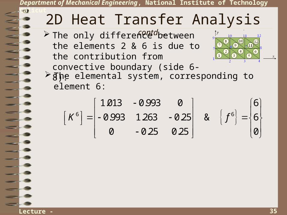
The only difference between the elements 2 & 6 is due to the contribution from convective boundary (side 6-8):
The elemental system, corresponding to element 6:
6 6
1.013 0.993 0 6
0.993 1.263 0.25 & 6
0 0.25 0.25 0
K f
Lecture - 03

36
Department of Mechanical Engineering, National Institute of Technology Calicut
2D Heat Transfer Analysis contd. …
1.277 0.237 0 0 1 0 0 0 0 0 0 0
0.237 2.554 0.237 0 0 2 0 0 0 0 0 0
0 0.237 2.554 0.237 0 0 2 0 0 0 0 0
0 0 0.237 0 0 0 0 0 0
1 0 0 0 1.25 0.25 0 0 0 0 0 0
0 2 0 0 0.25 2.50 0.25 0 0 0 0 0
0 0 2 0 0.25 0 0 0 0
0 0 0 0 0 0 0 0 0
0 0 0 0 0 0
0 -0.993
0 2.50 -0.25
-0.993 -0.25 1.263
1.29
0 0 0 0 0 0
0 0 0 0 0 0 0 0 0 0 0 0
0 0 0 0 0 0 0 0 0 0 0 0
0 0 0 0 0 0 0 0 0 0 0 0
Considering the contributions from elements 1 to 6, the global stiffness matrix is:
Lecture - 03

37
Department of Mechanical Engineering, National Institute of Technology Calicut
2D Heat Transfer Analysis contd. …
The only difference between the elements 7, 9 & 11 and 1 is due to the absence of contribution from convective boundary:
The elemental system, corresponding to element 7, 9 & 11:
1.25 0.25 1 0
0.25 0.25 0 & 0
1 0 1 0
e eK f
Lecture - 03
38
Department of Mechanical Engineering, National Institute of Technology Calicut
2D Heat Transfer Analysis contd. …
1.277 0.237 0 0 1 0 0 0 0 0 0 0
0.237 2.554 0.237 0 0 2 0 0 0 0 0 0
0 0.237 2.554 0.237 0 0 2 0 0 0 0 0
0 0 0.237 1.29 0 0 0 0.993 0 0 0 0
1 0 0 0 0 0 0 0 0
0 2 0 0 0 0 0
0 0 2 0 0 0 0
0 0 0 0.993 0 0 0 0 0 0
0 0 0 0 0 0 0
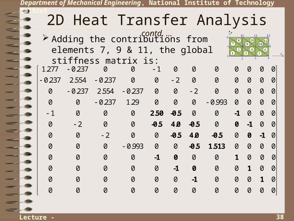
2.50 -0.5 -1
-0.5 4.0 -0.5 0 -1
-0.5 4.0 -0.5 0 -1
-0.5 1.513
-1 0 1 0 0
0 0 0 0 0 0 0 0 0
0 0 0 0 0 0 0 0 0 0
0 0 0 0 0 0 0 0 0 0 0 0
-1 0 1
-1 1
Adding the contributions from elements 7, 9 & 11, the global stiffness matrix is:
Lecture - 03
39
Department of Mechanical Engineering, National Institute of Technology Calicut
2D Heat Transfer Analysis contd. …
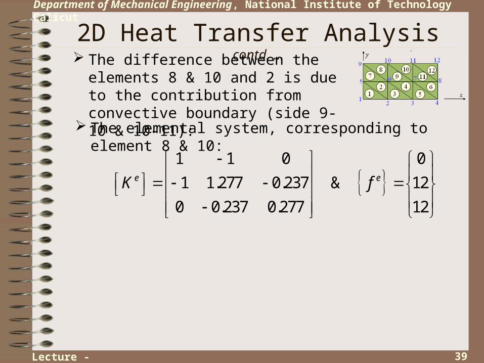
The difference between the elements 8 & 10 and 2 is due to the contribution from convective boundary (side 9-10 & 10-11):
The elemental system, corresponding to element 8 & 10:
1 1 0 0
1 1.277 0.237 & 12
0 0.237 0.277 12
e eK f
Lecture - 03
40
Department of Mechanical Engineering, National Institute of Technology Calicut
2D Heat Transfer Analysis contd. …
1.277 0.237 0 0 1 0 0 0 0 0 0 0
0.237 2.554 0.237 0 0 2 0 0 0 0 0 0
0 0.237 2.554 0.237 0 0 2 0 0 0 0 0
0 0 0.237 1.29 0 0 0 0.993 0 0 0 0
1 0 0 0 2.50 0.5 0 0 1 0 0 0
0 2 0 0 0.5 5.0 0.5 0 0 2 0 0
0 0 2 0 0 0.5 5.0 0.5 0 0 2 0
0 0 0 0.993 0 0 0.5 1.513 0 0 0 0
0 0 0 0 1 0 0 0 1.
277 0.237 0 0
0 0 0 0 0 2 0 0 0.237 2.554 0.237 0
0 0 0 0 0 0 2 0 0 0.237 2.277 0
0 0 0 0 0 0 0 0 0 0 0 0
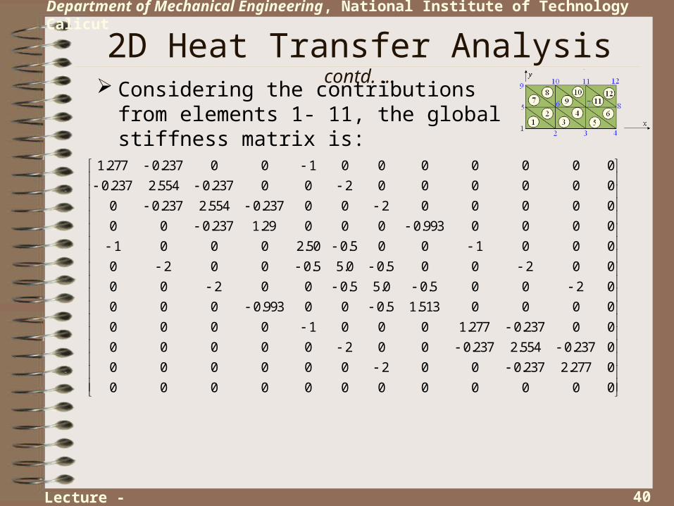
Considering the contributions from elements 1- 11, the global stiffness matrix is:
Lecture - 03

41
Department of Mechanical Engineering, National Institute of Technology Calicut
2D Heat Transfer Analysis contd. …
The difference between the elements 12 and 10 is due to the contribution from convective boundary (side 8-12):
The elemental system, corresponding to element 12:
1.013 0.993 0 6
0.993 1.29 0.237 & 18
0 0.237 0.277 12
e eK f
Lecture - 03

42
Department of Mechanical Engineering, National Institute of Technology Calicut
2D Heat Transfer Analysis contd. …
1.277 0.237 0 0 1 0 0 0 0 0 0 0
0.237 2.554 0.237 0 0 2 0 0 0 0 0 0
0 0.237 2.554 0.237 0 0 2 0 0 0 0 0
0 0 0.237 1.29 0 0 0 0.993 0 0 0 0
1 0 0 0 2.50 0.5 0 0 1 0 0 0
0 2 0 0 0.5 5.0 0.5 0 0 2 0 0
0 0 2 0 0 0.5 5.0 0.5 0 0 2 0
0 0 0 0.993 0 0 0.5 2.526 0 0 0 0.993
0 0 0 0 1
0 0 0 1.277 0.237 0 0
0 0 0 0 0 2 0 0 0.237 2.554 0.237 0
0 0 0 0 0 0 2 0 0 0.237 2.554 0.237
0 0 0 0 0 0 0 0.993 0 0 0.237 1.29
The complete global stiffness matrix is:
Transpose of the Global Force Vector:
12 24 24 18 0 0 0 12 12 24 24 18
Lecture - 03

43
Department of Mechanical Engineering, National Institute of Technology Calicut
2D Heat Transfer Analysis contd. …
1.277 0.237 0 0 1 0 0 0 0 0 0 0
0.237 2.554 0.237 0 0 2 0 0 0 0 0 0
0 0.237 2.554 0.237 0 0 2 0 0 0 0 0
0 0 0.237 1.29 0 0 0 0.993 0 0 0 0
1 0 0 0 2.50 0.5 0 0 1 0 0 0
0 2 0 0 0.5 5.0 0.5 0 0 2 0 0
0 0 2 0 0 0.5 5.0 0.5 0 0 2 0
0 0 0 0.993 0 0 0.5 2.526 0 0 0 0.993
0 0 0 0 1
0 0 0 1.277 0.237 0 0
0 0 0 0 0 2 0 0 0.237 2.554 0.237 0
0 0 0 0 0 0 2 0 0 0.237 2.554 0.237
0 0 0 0 0 0 0 0.993 0 0 0.237 1.29
Applying B.C.:
Transpose of the Global Force Vector:
12 24 24 18 0 0 0 12 12 24 24 18
Lecture - 04

44
Department of Mechanical Engineering, National Institute of Technology Calicut
2D Heat Transfer Analysis contd. …
2.554 0.237 0 2 0 0 0 0 0
0.237 2.554 0.237 0 2 0 0 0 0
0 0.237 1.29 0 0 0.993 0 0 0
2 0 0 5.0 0.5 0 2 0 0
0 2 0 0.5 5.0 0.5 0 2 0
0 0 0.993 0 0.5 2.526 0 0 0.993
0 0 0 2 0 0 2.554 0.237 0
0 0 0 0 2 0 0.237 2.554 0.237
0 0 0 0 0 0.993 0 0.237 1.29
Deleting rows & columns:
Modifying the Global Force Vector:
24 118.5 24 18 0 250 0 12 24 118.5 24 18
142.5 24 18 250 0 12 142.5 24 18
Lecture - 04
45
Department of Mechanical Engineering, National Institute of Technology Calicut
2D Heat Transfer Analysis contd. …
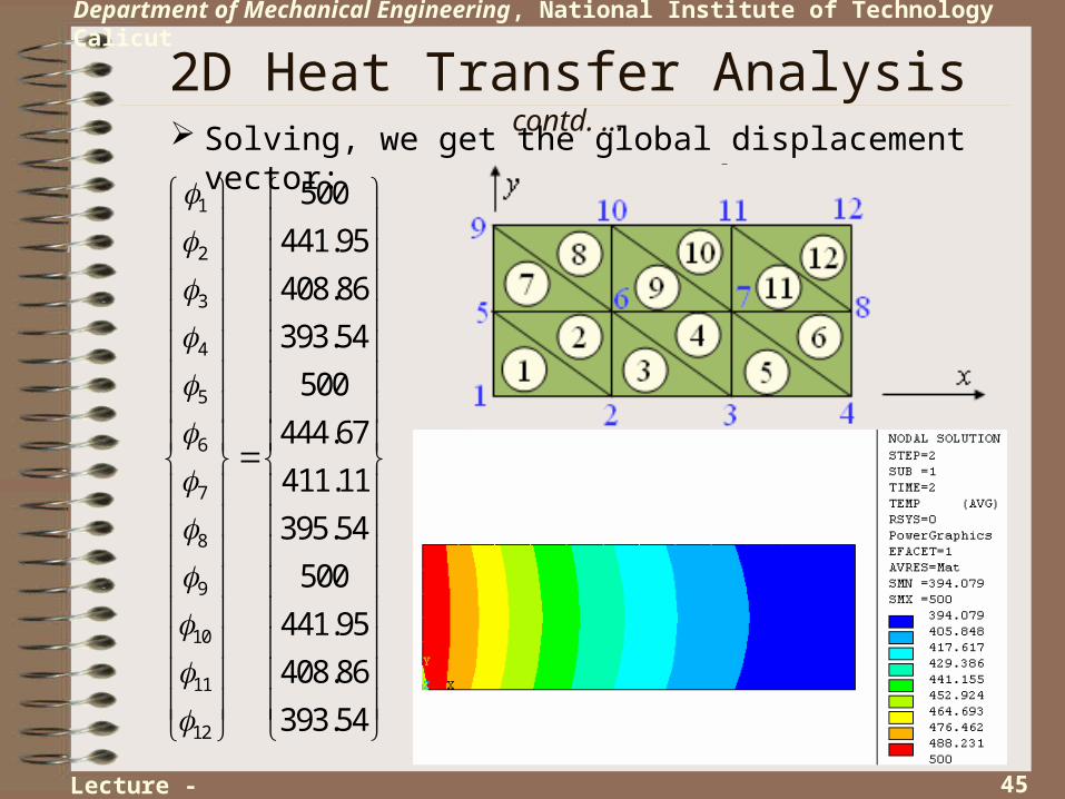
Solving, we get the global displacement vector:
1
2
3
4
5
6
7
8
9
10
11
12
500
441.95
408.86
393.54
500
444.67
411.11
395.54
500
441.95
408.86
393.54
Lecture - 04

46
Department of Mechanical Engineering, National Institute of Technology Calicut
2D Heat Transfer Analysis contd. …
We have the geometry and loading to be symmetric about the axis A-A.
Utilizing Symmetry to Reduce the Size of Problem:
A A
Hence, we only need to model one half (either above or below of A-A), provided, the suitable B.C. are applied at nodes on the axis A-A.
The B.C. to be applied is that there is no heat transfer across the axis A-A (in y-direction) – H.W..
0 at axis A-Aky
Lecture - 04

47
Department of Mechanical Engineering, National Institute of Technology Calicut
2D Heat Transfer Analysis contd. …
If there is a uniform heat generation throughout the domain, a minor modification is required in the formulation.
Problems with Heat Generation:
The only change will be for the right-side vector. The heat generation should add a term of the form:
This can be thought as if one-third of the heat generated in the element is lumped at each node (Valid only for linear triangle) – H.W.
e1
3e
i
Q QN d
k k
Cases of convection and temperature-dependent heat generation can be similarly handled, with the only difference that there will be a contribution towards the stiffness matrix in addition to the change in right-side vector – H.W.
Lecture - 04

48
Department of Mechanical Engineering, National Institute of Technology Calicut
Concluding Remarks By using the 2D Heat Transfer problem, we have introduced
the topic of FE analysis of a scalar field in 2D.
Lecture - 04
The Galerkin W.R. formulation is used, while the weak form is obtained by using Green’s Lemma (instead of integration by parts in 1D).
As in case of 1D problems, the natural B.C. were introduced at the time of formulating the W.R. statement, while the essential B.C. were directly enforced in the global algebraic system, just before the solution.
The methodology demonstrated in this example can be used in case of any scalar field problems in 2D, while the extension to vector field problems (e.g., elastic stress analysis) is considered in the next chapter.
The method can be easily extended to problems in 3D domains, by choosing proper elements & shape functions.