How To: Perform a Process Capability Analysis Using STATGRAPHICS Centurion · The target resistivity for the wafers is 225, with an allowable range of 100 to 500. Step 1: Plot the

© 2005 by StatPoint, Inc. How to Perform a Process Capability Analysis - 1

How To: Perform a Process Capability Analysis

Using STATGRAPHICS Centurion

by

Dr. Neil W. Polhemus

July 17, 2005

Introduction For individuals concerned with the quality of the goods and services that they provide, comparing observed performance to established standards or specifications is an important activity. Determining one’s capability to meet whatever promises have been made, whether to the customer or to upper management, requires collecting data and conducting a statistical analysis of it. Such an activity is referred to as a Process Capability Analysis, and programs like STATGRAPHICS Centurion provide important tools to facilitate this type of analysis. Quality engineers have routinely divided data into two major categories:

(1) variable data, usually consisting of measurements made on a continuous scale. Variables such as strength, weight, length, and concentration are typical examples.

(2) attribute data, usually consisting of a non-quantitative appraisal. Examples are

PASS/FAIL evaluations and counts of customer complaints. Since the analysis of these two types of data is very different, this How To guide will restrict the discussion to variable data. A future guide will deal with the equally important topic of attribute capability analysis.

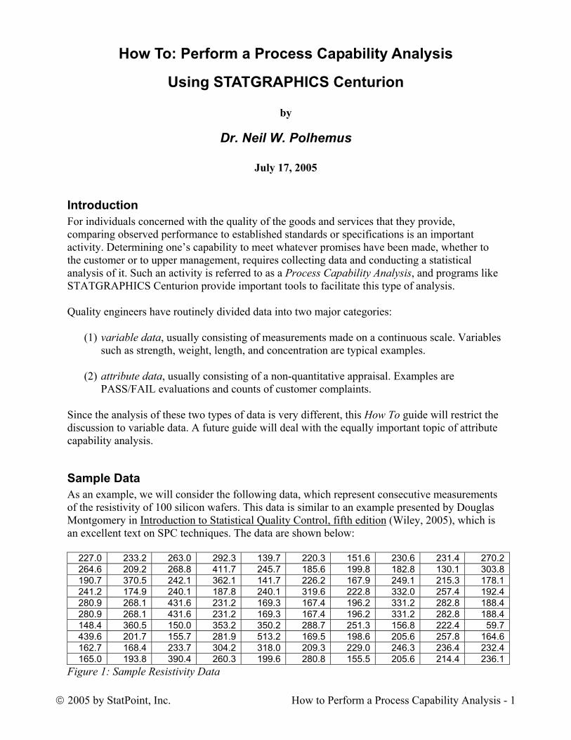
Sample Data As an example, we will consider the following data, which represent consecutive measurements of the resistivity of 100 silicon wafers. This data is similar to an example presented by Douglas Montgomery in Introduction to Statistical Quality Control, fifth edition (Wiley, 2005), which is an excellent text on SPC techniques. The data are shown below:

227.0 233.2 263.0 292.3 139.7 220.3 151.6 230.6 231.4 270.2264.6 209.2 268.8 411.7 245.7 185.6 199.8 182.8 130.1 303.8190.7 370.5 242.1 362.1 141.7 226.2 167.9 249.1 215.3 178.1241.2 174.9 240.1 187.8 240.1 319.6 222.8 332.0 257.4 192.4280.9 268.1 431.6 231.2 169.3 167.4 196.2 331.2 282.8 188.4280.9 268.1 431.6 231.2 169.3 167.4 196.2 331.2 282.8 188.4148.4 360.5 150.0 353.2 350.2 288.7 251.3 156.8 222.4 59.7439.6 201.7 155.7 281.9 513.2 169.5 198.6 205.6 257.8 164.6162.7 168.4 233.7 304.2 318.0 209.3 229.0 246.3 236.4 232.4165.0 193.8 390.4 260.3 199.6 280.8 155.5 205.6 214.4 236.1

Figure 1: Sample Resistivity Data

The target resistivity for the wafers is 225, with an allowable range of 100 to 500.

Step 1: Plot the Data When beginning to analyze a new set of data, it is always a good idea to plot it. Before blindly applying any statistical procedure, we must be sure that it makes sense to do so. In particular, most capability analysis procedures assume (at least by default) that the data are:

1. Stable over time, without major changes in the mean level or amount of variability. 2. Free from outliers. 3. Independent from sample to sample.

Procedure: Run Chart A good STATGRAPHICS Centurion procedure for plotting time-ordered data is the Run Chart, located under:

• If using the Classic menu: Plot – Time Sequence Plots – Run Charts. • If using the Six Sigma menu: Measure – Time Sequence Plots – Run Charts.

There are two run charts: one for individuals data such as that above, where each observation is taken at a different time (perhaps once every 15 minutes), and one for data taken in groups (perhaps 5 measurements at the end of each shift). After selecting the proper menu item, a data input dialog box will be displayed:

Figure 2: Data Input Dialog Box for Run Chart Procedure

Double-click on resistivity to enter it into the Observations field and press OK to display the following chart:


Run Chart

Observation

resi

stiv

ity

0 20 40 60 80 1000

100

200

300

400

500

600

median = 231.2

Figure 3: Run Chart for Resistivity Measurements

The run chart shows the observations plotted in time order. A solid line is drawn at the median of the sample. Important questions to ask of this data are: Does it appear to be stable throughout the sampling period? Has the level remained constant? Has the variability changed? To help answer this, try

double-clicking on the run chart to enlarge it and then press the Smooth/Rotate button on the analysis toolbar. On the subsequent dialog box, ask for a robust LOWESS smoother to be added to the chart:

Figure 4: Smooth/Rotate Dialog Box LOWESS stands for Locally Weighted Scatterplot Smoothing and is a technique that can be applied to any X-Y scatterplot to help visualize the relationship between the variables plotted on each axis. In this case, it shows that the level of the series has changed very little during the data collection period, perhaps rising slightly near the middle of the period:


Run Chart

Observation

resi

stiv

ity

0 20 40 60 80 1000

100

200

300

400

500

600

median = 231.2

Figure 5: Run Chart with LOWESS Smoother

The Run Chart procedure also displays in its Analysis Summary the results of two runs tests:

1. The runs above and below median test, which counts the number of groups of consecutive points that are all above the median or all below.

2. The runs up and down test, which counts the number of groups of consecutive points that

are all going up or all going down. Run Chart (Grouped Data) - resistivity Data variable: resistivity (resistivity of silicon wafers) 100 values ranging from 59.7 to 513.2 Median = 231.2 Test Observed Expected Longest P(>=) P(<=) Runs above and below median 48 50.0 4 0.69417 0.380326 Runs up and down 61 66.3333 4 0.918674 0.123665

The StatAdvisor This procedure is used to examine data for trends or other patterns over time. Four types of non-random patterns can sometimes be seen: 1. Mixing - too many runs above or below the median 2. Clustering - too few runs above or below the median 3. Oscillation - too many runs up and down 4. Trending - too few runs up and down The P-values are used to determine whether any apparent patterns are statistically significant. Since none of the P-values are less than 0.025, these are no significant non-random patterns at the 95% confidence level.

Figure 6: Run Chart Analysis Summary

If we suspect that the mean may have changed, we would expect to see:

• Less runs above and below the median than expected. • Less runs up and down than expected.



In fact, both observed counts are less than expected. However, the differences from expected behavior are not statistically significant, since the P values in the rightmost column are greater than or equal to 0.05. Therefore, there is no evidence to indicate any serious change in level over the sampling period. Several other observations are worthy of note:

1. With respect to the amount of variability, there also does not appear to have been much change.

2. With respect to the general distribution of the observations, there is a noticeable lack of

symmetry. Observations tend to deviate farther above the median than below it. This indicates the possible presence of skewness in the distribution, which means that the assumption of a normal distribution may not be tenable.

3. There are several points that may be potential outliers: one on the low side and several on

the high side. These points could have a big impact on the calculated capability of the process.

Procedure: Descriptive Time Series Methods There is one assumption we have not looked at yet: the assumption of independence between consecutive samples. This is an extremely important assumption, since indices such as Cpk are usually calculated from a moving range or a within-group standard deviation. Correlation between consecutive observations can lead to a badly underestimated process sigma and thus to an overly optimistic estimate of the process capability. With today’s automated data measurement systems, the short time intervals between samples makes this a real concern. The best way to look for correlation between consecutive measurements is to calculate the autocorrelation function of the data. To generate this plot:

• If using the Classic menu: select Describe – Time Series – Descriptive Methods. • If using the Six Sigma menu: select Forecast – Descriptive Time Series Methods.

Complete the data input dialog box as shown below:

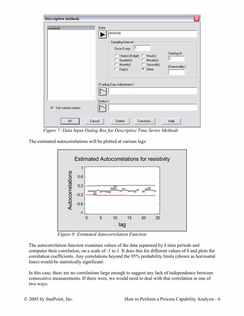
Figure 7: Data Input Dialog Box for Descriptive Time Series Methods The estimated autocorrelations will be plotted at various lags:

Estimated Autocorrelations for resistivity

lag

Auto

corr

elat

ions

0 5 10 15 20 25-1

-0.6

-0.2

0.2

0.6

1

Figure 8: Estimated Autocorrelation Function

The autocorrelation function examines values of the data separated by k time periods and computes their correlation, on a scale of -1 to 1. It does this for different values of k and plots the correlation coefficients. Any correlations beyond the 95% probability limits (shown as horizontal lines) would be statistically significant. In this case, there are no correlations large enough to suggest any lack of independence between consecutive measurements. If there were, we would need to deal with that correlation in one of two ways:


1. Build a time series model to represent the dynamics of the process.

2. Increase the time interval between samples to eliminate the correlation. Dealing with autocorrelated measurements will be the subject of a later How To guide.

Step 2: Deal with Any Non-Normality in the Data The apparent skewness in the data is troubling, since most statistical procedures assume that the data follow a normal distribution. If normality is not tenable, we must either:

1. Fit a different distribution to the data and adapt our statistical procedures to that distribution.

2. Find a transformation of the data such that normality is a reasonable assumption in the

transformed metric. Procedure: Distribution Fitting The first step here is to perform a formal test for normality, since we don’t want to complicate the analysis unless we really need to. In STATGRAPHICS Centurion, a formal test for normality may be conducted by selecting:

• If using the Classic menu: Describe – Distribution Fitting – Fitting Uncensored Data. • If using the Six Sigma menu: Analyze – Variable Data - Distribution Fitting – Fitting

Uncensored Data. The data input dialog box is shown below:

Figure 9: Data Input Dialog Box for Distribution Fitting

Part of the standard default output is the Shapiro-Wilks test:


Tests for Normality for resistivity Test Statistic P-Value Shapiro-Wilks W 0.941697 0.000372934

The StatAdvisor This pane shows the results of several tests run to determine whether resistivity can be adequately modeled by a normal distribution. The Shapiro-Wilks test is based upon comparing the quantiles of the fitted normal distribution to the quantiles of the data. Since the smallest P-value amongst the tests performed is less than 0.05, we can reject the idea that resistivity comes from a normal distribution with 95% confidence.

Figure 10: Tests for Normality Output from Distribution Fitting Procedure A P-Value below 0.05, as in the above table, rejects the hypothesis that the data come from a normal distribution.

To select an alternative distribution, press the Tabular Options button on the analysis toolbar and select Comparison of Alternative Distributions. This option will fit a wide variety of distributions and order them according to a goodness-of-fit criterion, such as the Anderson-Darling A2 statistic:

Comparison of Alternative Distributions Distribution Est. Parameters KS D A^2 Loglogistic 2 0.0477508 0.289605 Largest Extreme Value 2 0.0563468 0.377902 Lognormal 2 0.0553747 0.422962 Inverse Gaussian 2 0.0557318 0.472093 Birnbaum-Saunders 2 0.0562796 0.477558 Gamma 2 0.0631831 0.62267 Laplace 2 0.0806926 1.02854 Logistic 2 0.0746663 1.07395 Normal 2 0.103212 1.77192 Weibull 2 0.104577 2.00503 Smallest Extreme Value 2 0.17388 5.49967 Exponential 1 0.4202 22.9211 Pareto 1 0.58171 40.9609 Uniform 2 0.308049

The StatAdvisor This table compares the goodness-of-fit when various distributions are fit to resistivity. You can select other distributions using Pane Options. According to the Anderson-Darling A^2 statistic, the best fitting distribution is the loglogistic distribution. To fit this distribution, press the alternate mouse button and select Analysis Options.

Figure 11: Comparison of Alternative Distributions Output from Distribution Fitting Procedure According to both the Kolmogorov-Smirnov D statistic and the Anderson-Darling A2 statistic, the loglogistic distribution seems to fit the data best. Using Analysis Options, you can specify up to 5 distributions to plot at the same time. The plot below shows the five best-fitting distributions:


Histogram for resistivity

resistivity

frequ

ency

DistributionBirnbaum-SaundersInverse GaussianLargest Extreme ValueLoglogisticLognormal

0 100 200 300 400 500 6000

4

8

12

16

20

24

Figure 12: Five Fitted Distributions

The best-fitting loglogistic distribution is the one with the highest peak. Procedure: Power Transformations The second method for dealing with non-normal data is to seek a transformation of the data that normalizes it. The most common transformations used in statistics are power transformations of the form Yp

in which the data are raised to the p-th power. This covers common transformations such as:

• a square root, for p = 0.5 • a reciprocal, for p = -1 • a logarithm, for p=0

Although the last is not obvious, it can be shown mathematically that as p approaches 0, the effect on the distribution of the data is the same as taking logs. STATGRAPHICS Centurion contains a special procedure for helping determine a good transformation to apply to a given set of data. To run it:

• If using the Classic menu: select Describe – Numeric Data – Power Transformations. • If using the Six Sigma menu: select Analyze – Variable Data – Distribution Fitting –

Power Transformations. The data input dialog box is shown below:


Figure 13: Data Input Dialog Box for Power Transformations

Using the methods of Box and Cox, the procedure will select an optimal transformation of the form ( ) 1

2λλ+=′ YY

Usually, the shift parameter λ2 is set equal to 0: Power Transformations Data variable: resistivity (resistivity of silicon wafers) Number of observations = 100 Box-Cox Transformation Power (lambda1): 0.237 Shift (lambda2): 0.0 (optimized) Geometric mean = 229.229 Approximate 95% confidence interval for power: -0.154 to 0.662

Figure 14: Power Transformations Analysis Summary The above table indicates that the optimal power transformation for this data is to raise it to the 0.237 power. However, the 95% confidence for the power extends from -0.154 to 0.662, covering both the logarithm and the square root. An interesting plot is available in the Power Transformations procedure by pressing the

Graphics Options button on the analysis toolbar and selecting Skewness and Kurtosis Plot:


skewnesskurtosis

Skewness and Kurtosis Plotlambda2 =0.0

lambda1-2 -1 0 1 2

-8

-4

0

4

8

Figure 15: Plot of Standardized Skewness and Kurtosis

This plot shows the standardized skewness and standardized kurtosis values for the data after transforming it according to different powers. If a power transformation successfully normalizes the data, both the skewness and kurtosis should fall within the two horizontal lines. At the optimal power of 0.237, shown as the middle vertical line, skewness is essentially 0. However, the kurtosis is right on the boundary of being unacceptable. In this case, the Box-Cox procedure has not done a very good job in normalizing the data. Further insight can be gained by selecting Normal Probability Plot from the Graphics Options menu (within the Power Transformations procedure). This option creates a normal probability plot for the transformed data, using the derived optimum power:

Figure 16: Normal Probability Plot for Transformed Data

If the transformation effectively normalized the data, the transformed values should fall approximately along a straight line. In this case, some obvious curvature may be seen, as well as an apparent outlier. It is that aberrant data value that we will focus on next.


Step 3: Identify and Deal with any Outliers in the Data It is not uncommon to observe a data value that does not appear to belong with the rest. Ideally, the analyst would have the opportunity to go back to the source of the data and identify an assignable cause for the unusual value that could then be corrected. In such a case, one would be fully justified in removing such an observation and performing the capability analysis on the remainder. Sometimes, follow-up is impossible, so that we must make the best decision we can about whether to include the observation in the analysis. Obviously, erroneously removing an outlier that represents a repeating event would lead to an overly optimistic estimate of the process capability. On the other hand, keeping an observation that was incorrectly recorded could lead to a seriously pessimistic estimate of capability. In such cases, some statistical help can be useful in quantifying the likelihood that the suspect observation actually belongs with the rest. Procedure: Outlier Identification Our next step in the analysis will be to take the transformed data and pass it through the Outlier Identification procedure. To run this procedure:

• If using the Classic menu: select Describe – Numeric Data – Outlier Identification. • If using the Six Sigma menu: select Analyze – Variable Data – Outlier Identification.

The data input dialog box is shown below:

Figure 17: Data Input Dialog Box for Outlier Identification

Notice that we have used STATGRAPHICS’ “on-the-fly” transformation feature, so that we do not have to change the original datasheet. The procedure creates a helpful Outlier Plot that shows each point together with the sample mean plus and minus 1, 2, 3 and 4 standard deviations:


Outlier Plot with Sigma LimitsSample mean = 3.63584, std. deviation = 0.27253

Row number

resi

stiv

ity^0

.237

0 20 40 60 80 1002.5

2.9

3.3

3.7

4.1

4.5

4.9

-4-3-2-101234

Figure 18: Outlier Plot from Outlier Identification

All of the points are within 3 standard deviations of the mean, except for the suspect point, which is almost 4 standard deviations low. The Analysis Summary table lists the 5 largest and 5 smallest values, together with the result of Grubbs’ test: Outlier Identification - resistivity^0.237 Data variable: resistivity^0.237 100 values ranging from 2.63576 to 4.38872 Number of values currently excluded: 0 Location estimates Sample mean 3.63584 Sample median 3.633 Trimmed mean 3.62134 Winsorized mean 3.62781

Trimming: 15.0% Scale estimates Sample std. deviation 0.27253 MAD/0.6745 0.254737 Sbi 0.261106 Winsorized sigma 0.276897

Sorted Values Studentized Values Studentized Values Modified Row Value Without Deletion With Deletion MAD Z-Score 70 2.63576 -3.66962 -3.97077 -3.91478 19 3.17018 -1.70866 -1.74335 -1.81685 5 3.22412 -1.51073 -1.53625 -1.60509 25 3.235 -1.4708 -1.49473 -1.56238 61 3.27062 -1.34012 -1.35931 -1.42257 ... 14 4.16539 1.94309 1.99151 2.08997 53 4.21225 2.11504 2.17582 2.27393 43 4.21225 2.11504 2.17582 2.27393 71 4.23063 2.18246 2.24866 2.34607 75 4.38872 2.76256 2.89118 2.96669

Grubbs' Test (assumes normality) Test statistic = 3.66962 P-Value = 0.0146907

Figure 19: Outlier Identification Analysis Summary


Grubbs’ test takes the most extreme data value and expresses it in terms of the number of standard deviations away from the mean. In this case, the most extreme point is 3.67 standard deviations below the mean. It then computes a P-Value to determine how significant the outlier is. A P-Value of .05 or below indicates that the point is a significant outlier at the 5% significance level. It this case, the outlier is nearly significant at the 1% level. We would therefore conclude that it is very unlikely that the suspect data value comes from the same population as the rest. To tentatively remove the point from the calculations, we can return to the outlier plot, click on

the suspect point, and press the Exclude button on the analysis toolbar. The mean and standard deviation will then be recalculated using the remaining 99 observations, and the plot will be automatically redrawn:

Outlier Plot with Sigma LimitsSample mean = 3.64594, std. deviation = 0.254405

Row number

resi

stiv

ity^0

.237

0 20 40 60 80 1002.6

3

3.4

3.8

4.2

4.6

5

-4-3-2-101234

Figure 20: Outlier Plot after Removal of Suspect Data Value

At the same time, Grubbs’ test will be rerun for the most extreme data value in the remaining sample:

Sorted Values Studentized Values Studentized Values Modified Row Value Without Deletion With Deletion MAD Z-Score 70 X 2.63576 -3.97077 19 3.17018 -1.87011 -1.91435 -1.81936 5 3.22412 -1.65807 -1.69055 -1.60731 25 3.235 -1.6153 -1.64572 -1.56454 61 3.27062 -1.47531 -1.49966 -1.42453 ... 93 4.11328 1.83697 1.87919 1.888 14 4.16539 2.04182 2.09767 2.09286 53 4.21225 2.22602 2.29665 2.27708 43 4.21225 2.22602 2.29665 2.27708 71 4.23063 2.29824 2.37539 2.34931 75 4.38872 2.91967 3.07247 2.97078

Grubbs' Test (assumes normality) Test statistic = 2.91967 P-Value = 0.286059

Figure 21: Grubbs’ Test for Remaining 99 Data Values The P-Value for the most extreme point is now well above 0.05, indicating that there are no outliers remaining.


Step 4: Rerunning the Earlier Procedures Having determined that an outlier is present in the data, we should now redo the earlier analyses without the outlier. This is extremely easy to do in STATGRAPHICS Centurion, since you can

activate any earlier window and press the Input button on the analysis toolbar to change the input data selection. For example, to determine the best-fitting distribution, return to the Distribution Fitting window and modify the data input dialog box as shown below:

Figure 22: Modified Data Input Dialog Box

By entering resistivity > 100 in the Select field, we will analyze only the 99 data values that we want. The resulting comparison of distributions now shows:

Comparison of Alternative Distributions Distribution Est. Parameters KS D A^2 Largest Extreme Value 2 0.0628601 0.317665 Loglogistic 2 0.0536372 0.394557 Lognormal 2 0.0532022 0.404248 Inverse Gaussian 2 0.0543899 0.413534 Birnbaum-Saunders 2 0.0543173 0.425763 Gamma 2 0.0701443 0.761322 Laplace 2 0.0873128 1.23229 Logistic 2 0.0783686 1.24552 Normal 2 0.10881 2.00441 Weibull 2 0.108898 2.26449 Smallest Extreme Value 2 0.179501 5.74851 Exponential 1 0.427645 23.4344 Pareto 1 0.590797 40.85 Uniform 2 0.399389

The StatAdvisor This table compares the goodness-of-fit when various distributions are fit to resistivity. You can select other distributions using Pane Options. According to the Anderson-Darling A^2 statistic, the best fitting distribution is the largest extreme value distribution. To fit this distribution, press the alternate mouse button and select Analysis Options.

Figure 23: Comparison of Distributions after Removing Outlier


The Anderson-Darling statistic suggests that the largest extreme value distribution would now be best, although the loglogistic distribution is extremely close. A plot of the fitted distributions shows how close the top two choices are:

Histogram for resistivity

resistivity

frequ

ency

DistributionBirnbaum-SaundersInverse GaussianLargest Extreme ValueLoglogisticLognormal

0 100 200 300 400 500 6000

4

8

12

16

20

24

Figure 24: Fitted Distributions after Removing Outlier

Making the same changes to the Power Transformations procedure creates the following plot:

skewnesskurtosis

Skewness and Kurtosis Plotlambda2 =0.0

lambda1-2 -1 0 1 2

-4

-2

0

2

4

Figure 25: Skewness and Kurtosis Plot after Removing Outlier

The optimal power has moved to -0.53, or essentially a reciprocal square root. At that power, both the standardized skewness and standardized kurtosis are well within the expected range. Note also that the normal probability plot is now more like that expected for data from a normal distribution:


Normal Probability Plot for transformed resistivitylambda1 = -0.53, lambda2 = 0.0

transformed resistivity

perc

enta

ge

7200 7300 7400 7500 76000.1

15

2050809599

99.9

Figure 26: Normal Probability Plot after Removing Outlier

Step 5: Calculating Process Capability We are now ready to calculate the capability of our process. Two procedures are available for doing so: the Process Capability Analysis procedure, which has many options, and the Capability Assessment SnapStat, which has limited options but produces a single page of preformatted output. In this case, we’ll use the former, which you can access by:

• If using the Classic menu: select SPC – Capability Analysis – Variables – Individuals. • If using the Six Sigma menu: select Analyze – Capability Analysis – Variables –

Individuals. A similar procedure is available for grouped data. The data input dialog box should be completed as shown below:

Figure 27: Data Input Dialog Box for Process Capability Analysis


Notice the following:

• We have entered the specification limits and the target (nominal) values. At least one

of the USL and LSL fields must have an entry. • We have used the Select field to exclude the identified outlier through a Boolean

expression that will select only data values that are greater than 100. When the analysis window first appears, a histogram will be drawn with statistics based on a normal distribution:

NormalMean=242.618Std. Dev.=75.2608

Cp = 0.91Pp = 0.89Cpk = 0.65Ppk = 0.63K = 0.09

Process Capability for resistivity LSL = 100.0, Nominal = 225.0, USL = 500.0

resistivity

frequ

ency

DPM = 29,360

0 100 200 300 400 500 6000

4

8

12

16

20

24

SQL = 3.39

Figure 28: Capability Analysis Based on Normal Distribution

Assuming a normal distribution, which we know is not appropriate, yields an estimate of 29,360 wafers outside the specification limits, for a Sigma Quality Level of 3.39. If we select Analysis Options, we can change the assumed distribution or specify a transformation:


Figure 29: Capability Analysis Options Dialog Box Based upon what we know, we could either:

1. Select the Largest Extreme Value radio button. 2. Select the Power radio button in the Data Transformation section and enter the

transformation we wish to use.

Taking the first approach yields:

Largest Extreme ValueMode=209.295Scale=55.532

Cp = 0.94Pp = 0.95Cpk = 0.84Ppk = 0.85K = 0.03

Process Capability for resistivity LSL = 100.0, Nominal = 225.0, USL = 500.0

resistivity

frequ

ency

DPM = 6,092SQL = 4.01

0 100 200 300 400 500 6000

4

8

12

16

20

24

Figure 30: Fitted Largest Extreme Value Distribution The estimated defects per million is now only 6,902, much less than when a normal distribution was assumed. The Sigma Quality Level is 4.01.


One final note concerning the capability indices is in order. A very commonly used index for process capability is Cpk, defined for data from a normal distribution by

⎟⎠⎞

⎜⎝⎛ −−

=σ

μσ

μˆ3

ˆ,

ˆ3ˆ

min LSLUSLCPK

where μ̂ is the estimated process mean and σ̂ is the estimated process standard deviation. This is essentially a ratio of the distance to the nearer specification limit divided by the distance from the mean to the point on the normal curve leaving only 0.135% in the tail. When a normal distribution is not appropriate, STATGRAPHICS Centurion gives you two options for how to compute the indices (selected using the Edit – Preferences dialog box):

1. Use Corresponding Z-Scores: With this method, the location of the sample mean and the specification limits are converted to standardized normal Z-scores. The capability index is then calculated from those Z-scores. This insures that a given value of Cpk corresponds to the same percentage beyond the specification limit as when the data follow a normal distribution. Thus rules such as desiring Cpk to be at least 1.33 still give the same assurance regarding DPM (defects per million).

2. If Use Distance between Percentiles is selected, then the sample mean and specification

limits are replaced by corresponding percentiles of the fitted distribution. The interpretation of Cpk as a ratio of two distances is maintained, but a Cpk of 1.33 will not correspond to the same DPM as for a normal distribution.

By default, STATGRAPHICS Centurion uses the first option, which maintains the expected relationship between the capability indices, DPM, and the Sigma Quality Level. This latter quantity is often used in Six Sigma projects as a summary of how well the process is performing, with an SQL of 6 representing “world class” quality or 3.4 defects per million.

Conclusion This document has discussed some of the difficulties that can arise in practice when performing a process capability analysis. Non-normality and outliers are common problems, and failure to deal with them properly can give a very misleading picture of how capable a process is. It should be emphasized that the question of what distribution to use for a particular variable and whether and how to transform it should not be done every time a new sample of data is analyzed. Rather, a protocol should be established for how to handle a specific variable, based on some initial detailed study of a large amount of data. Then, whenever that variable is analyzed, the same protocol should be applied. Otherwise, the random variability in each sample of data will be magnified by affecting not only the capability estimates but also the manner in which they are obtained. In short, study your process closely, establish a protocol for handling data obtained from it, and then stick by that protocol. Note: The author welcomes comments about this guide. Please address your responses to [email protected].


mailto:[email protected]

Documents

How To: Perform a Process Capability Analysis Using STATGRAPHICS Centurion · The target resistivity for the wafers is 225, with an allowable range of 100 to 500. Step 1: Plot the