HOW TO COMBINE INDUCTIVE AND DEDUCTIVE APPROACHES … · HOW TO COMBINE INDUCTIVE AND DEDUCTIVE APPROACHES TO PREDICTION? Pablo F. Dornes1,2 1Centre for Hydrology, University of Saskatchewan,

HOW TO COMBINE INDUCTIVE AND DEDUCTIVEAPPROACHES TO PREDICTION?

Pablo F. Dornes1,2

1Centre for Hydrology, University of Saskatchewan, Saskatoon, SK, Canada

2Now at Facultad de Ciencias Exactas y Naturales.Universidad Nacional de La Pampa, Santa Rosa, La Pampa, Argentina

10.1 ABSTRACT

The implementation of a new modelling philosophy based on thecombination of inductive and deductive reasoning approaches forpredicting snowcover ablation and snowmelt runoff is illustrated. Aninductive (i.e. top-down) modelling approach was used for representinglandscape heterogeneity, whereas a deductive (i.e. bottom-up) approachwas applied for detailed snowmelt process descriptions. Physically basedhydrological land surface simulations, using distributed initial conditionsof snowcover and incoming solar radiation, showed an appropriaterepresentation of both the basin hydrographs and the snowcover ablation.Aggregated simulations were unable to describe the dynamics of the basinstreamflow when the runoff response was largely governed by solarradiation. When temperature was a key factor in the onset of melt, thedifferences were less. Results indicate that the number of model unitsshould be in concordance with the association between initial snow waterequivalent (SWE) and melt energy to adequately represent the landscapeheterogeneity in subarctic environments. The modelling methodologycapitalizes on the strength of both modelling approaches, and appears to bean effective method to reduce the size of the parameter sets and still retainphysical consistency. Therefore it is an appropriate methodology forapplying physically based hydrological models in poorly or ungaugedbasins such as complex subarctic environments.

153

10

10.2 RÉSUMÉ

La mise en œuvre d’une nouvelle philosophe de modélisation basée sur lacombinaison d’approches de raisonnement inductif et déductif pour laprévision de l’ablation nivale et du ruissellement nival est illustrée. Uneapproche de modélisation inductive (c.-à-d. descendante) a été utilisée pourreprésenter l’hétérogénéité du paysage, tandis qu’une approche déductive (c.à d. ascendante) a été appliquée pour les descriptions détaillées du processusde fonte nivale. Des simulations hydrologiques à la surface des sols, à basephysique et reposant sur des conditions initiales distribuées de manteauneigeux et de rayonnement solaire incident, ont révélé une représentationappropriée à la fois des hydrogrammes de bassin et de l’ablation nivale. Lessimulations globales n’ont pas permis de décrire la dynamique du débit dubassin versant lorsque la réaction de ruissellement était en grande partiedictée par le rayonnement solaire. Lorsque la température était un facteur cléau début de la fonte, les différences étaient moindres. Les résultats indiquentque le nombre d’unités de modèle devrait correspondre à l’association entrel’équivalent en eau de la neige (EEN) initial et l’énergie de la fonte pourreprésenter de manière suffisante l’hétérogénéité du paysage en milieusubarctique. La méthode de modélisation mise sur la force des deuxapproches de modélisation et semble constituer une méthode efficace pourréduire la taille des séries de paramètres tout en conservant une cohérencephysique. Par conséquent, il s’agit d’une méthode appropriée pourl’application de modèles hydrologiques à base physique aux bassins nonjaugés ou pauvrement jaugés, par exemple en milieu subarctique complexe.

10.3 INTRODUCTION

Making reliable statements about modelling hydrological processes atdifferent spatial and temporal scales is a crucial aspect to hydrology andremains a major challenge in hydrological research. The main constraint isto consider and evaluate the effects of the numerous complex interactionsamong hydrological inputs, landscape properties, and initial conditions.Over the years there have been attempts to make modelling tools morerigorous and representations of hydrological processes more realistic,through incorporation of spatial and physical descriptions. While moresophisticated models result, they continue to suffer from restrictiveassumptions, particularly the representation of landscape heterogeneity and

154

Putting Prediction in Ungauged Basins into Practice Dornes

both parameter and modelling equifinality that result from transferring pointscale observations and process descriptions to basin scales (Beven, 2002).Traditionally, two main approaches to model building have been applied,deductive and inductive. The deductive or bottom-up approach,conceptualizes a model structure that is based on the belief that the physicalsystem can be described by deterministic mathematical equations (Young,2003). This deductive approach assumes that process knowledge acquiredon small spatial and temporal scales can be used to predict the overall basinresponse by means of up-scaling small-scale process understanding. Thiswas first outlined by Freeze and Harlan (1969) for a distributed physicallybased hydrological model. Typically, this means that physically basedequations developed at laboratory or point-scale are usually applied todescribe hydrological processes at larger scales (i.e. basin models).Conversely, the inductive or top-down approach avoids theoreticalpreconceptions as much as possible in the initial stages of the analysis(Klemeš, 1983). The model structure is not pre-specified; rather it is inferredfrom the observational data. The approach consists of deriving behaviourthrough an analysis of its response based on the rationale that information ormodel complexity should be only added when the prior conceptualizationwas not able to describe the processes of interest. The inductive approachtherefore has a model structure which is inferred from the data, whereas themodel conceptualization is based on the predominant processes at thecatchment scale (Sivapalan et al., 2003a; Littlewood et al., 2003).Both approaches are challenged by scaling issues related to the nonlinearityof the hydrological processes (Beven, 2001). Limitations of the deductiveapproach are [1] that processes important at one scale may not necessarily beimportant at other scales (Blöschl and Sivapalan, 1995), and [2] the problemsof model equifinality and parameter identifiability that result from explicitlandscape representations and incorporation of detailed process descriptions(Beven, 2000; 2006). Distributed physically based models have large degreesof freedom since many parameters and initial conditions need to be set, andconsequently, these models rely on calibration to account for the lack ofknowledge in representing the landscape heterogeneity and to compensate forthe insufficient understanding of physical processes and their interactions(Beven, 2006; Kirchner, 2006; McDonnell et al., 2007). Thus, fullydistributed physically based models are usually restricted to small areas due

155

10 – How to combine inductive and deductive approaches to prediction?

to their large requirements for data and computational time (Todini, 2007).Limitations of the inductive modelling approach are [1] it attempts to identifyprocesses directly at the scales of interest, [2] it interprets these in terms ofproperties and processes occurring at finer scales, and [3] since data areusually rather limited, only simple and often physically unrealistic modelscan be inferred solely from the data (Sivapalan et al., 2003a).

Aided by increased computing power, increased process understanding, andthe availability of digital terrain attributes, the most widely used modellingphilosophy is the deductive approach describing a hydrological system bydeterministic mathematical equations founded on well-known scientificlaws (Beven, 2002; Ratto et al., 2007). Though these models have complexprocess descriptions, they often do not properly account for landscapeheterogeneity and drainage basin hydrological dynamics (Beven, 1989;Kirchner, 2006; Savenije, 2009).

One challenge for the hydrological modelling community is to produceaccurate and reliable predictions in ungauged or poorly gauged basins. Thechallenge is even more difficult in areas with limited data, such as in coldregions due to the limited gauging of subarctic and arctic environments.While the application of distributed and physically based models in suchenvironments is restricted due to the lack of data, models based uponphysically based process descriptions offer a valid approach to extrapolationbeyond available observations.

Both inductive and deductive modelling methodologies have limitationswhen scaling is needed to adapt the model structure, the process descriptions,and the observational data. The methodology of this study seeks to combinethe strengths of the two approaches used in hydrological modelling. Theobjective of this work is to demonstrate this combined modelling approachfor predicting snowcover depletion and snowmelt runoff in cold regionenvironments with limited input data while retaining physical integrity withinthe processes representation. In order to reduce the predictive uncertainty ofphysically based models in ungauged basins, this study seeks an appropriatemodel complexity, one that is physically based and parametrically efficient,for an area with limited data and that would allow both the scaling from pointscale observations to catchment scale models and the identification of stablelandscape based model parameterizations.

156


10.4 STUDY AREA

The study area is the Wolf Creek Research Basin (WC) which lies on theinterior edge of the Coast Mountains at approximately 61° N latitude,155° W longitude (Figure 10.1). The WC basin encompasses an area of195 km2 and is located in the northwest of Canada 15 km south of Whitehorse.The basin is part of the southern mountainous headwaters of the Yukon RiverBasin and has a generally northeasterly aspect with elevations ranging from800 to 2035 m a.s.l. and a median elevation of 1325 m a.s.l. The climate issub-arctic continental which is characterized by a large variation intemperature, low relative humidity, and relatively low precipitation. Meanannual temperature is in the order of -3°C with summer and winter extremesof 25° and -40°C respectively. Mean annual precipitation is 300 to 400 mmwith approximately 40 percent falling as snow (Pomeroy et al., 1999). The

157


Figure 10.1 Wolf Creek Research Basin (WC). (a) Topographic map. GB: Granger Basin.Circles indicate meteorological stations (PLT: Plateau, ALP: Alpine, BB: Back-brush, and F: Forest), (b) Land-cover map. Squares indicate streamflow gaugestations. (UWC: Upper Wolf Creek, GC: Granger Creek, CL: Coal Lake, andWCAH: Wolf Creek Alaska Highway). Inset shows the location in Canada.

WC basin is within the sporadic discontinuous permafrost zone, andpermafrost is present in north facing (NF) slopes, poorly drained areas, orareas with significant organic layers. In permafrost areas and the riparianzones, soils are capped by an organic layer up to 0.4 m thick consisting of peat,lichens, mosses, sedges, and grasses (Carey and Quinton, 2005). The WC basin spans three major environments separated primarily on agradient of elevation (Figure 10.1b). The boreal forest (spruce, pine, aspen)is found in lower areas (800-1300 m a.s.l.), subalpine taiga (shrub tundra) isfound at mid-elevations (1300-1800 m a.s.l.), while alpine tundra (shortshrubs, forbs, and bare rock) dominates high elevation areas(1800-2035 m a.s.l.). These ecological zones cover 22, 58 and 20% of thebasin area respectively (Francis, 1997). Granger Basin (GB) is a small 8 km2

sub-basin located in the northwest edge of WC basin (see Figure 10.1a)drained by Granger Creek with a length of approximately 3 km.Physiographically, GB is characterized by a northeasterly aspect and rangesin elevation from 1310 to 2035 m a.s.l; it encompasses the alpine tundra andshrub tundra environments. The selection of GB resulted from the extensiveexisting field observations of the WC research project (Janowicz, 1999)which included landscape snow survey transects measured on a daily basisduring snowmelt, meteorological and soil moisture observations performedin different landscapes (e.g., UB: upper basin, PLT: plateau area, NF and SF:north and south facing slopes, and VB: valley bottom) within the basin(Janowicz, et al., 2002; Pomeroy et al., 2003; McCartney et al., 2006;Bewley et al., 2007).

10.5 MODELLING STRATEGY

Prediction of snowcover depletion and spring melt runoff in subarctic andarctic basins is challenging due to the combination of their remote locationand the importance of the winter processes (e.g. snow accumulation andredistribution). Streamflow in these regions is generally difficult to gaugewell due to winter inaccessibility (Pomeroy et al., 2007). The conceptual methodology of this study is based on combining thestrengths of the two approaches used in hydrological modelling. Aninductive approach was used for the identification of the spatial model units(i.e. basin segmentation) based on a basin wide understanding of the mainhydrological responses, while a deductive modelling approach, based on a

158


detailed process description, was applied in each of the model units togenerate the physically based forcing data and process representations. Thisapproach follows those ideas proposed by Dooge (1986) about the need todefine parameterization of microscale effects and the search for macroscalelaws to properly describe the dynamics of intermediate size systemscategorized by both high complexity and degree of organization. The modelling methodology of this study consists of distributed landscapebased simulations of snowcover ablation and snowmelt runoff using a landsurface hydrological (LSH) model in the WC basin. The simulation periodincluded the 2002 and 2003 snowmelt seasons. The modelling techniquesinvolved up-scaling exercises from landscape based simulations performedwith two models, a small-scale hydrological model, and a land surfacescheme (LSS) (Dornes et al., 2008a; 2008b) in GB. These models were usedto investigate the effects of including explicit landscape representation andthe effects of varying degrees of spatial complexity in the initial conditionsand forcing data on snowmelt simulations. In order to evaluate theperformance of the distributed landscape based model in WC, model resultswere compared to simulations using an aggregated modelling approachassuming a basin average initial SWE and incoming solar radiation whichwas not corrected for slope and aspect effects.

Model description

As part of the MEC (Modélisation Environmentale Communautaire)developed by Environment Canada, the MEC – Surface and Hydrology(MESH; Pietroniro et al., 2007) is a stand-alone LSH model configurationthat couples an LSS, specifically the Canadian Land Surface Scheme(CLASS) with hydrological routing schemes. Representation of spatialheterogeneity is based on a mosaic approach using the Group Response Unit(GRU) concept (Kouwen et al., 1993) where areas with similar land cover,soils, etc., are grouped with no requirement for grids or sub-basins to behydrologically homogenous. The implicit assumption is that each individualcomponent of the land surface mosaic has the same response for giveninputs of energy and water. GRUs are grouped together into predefinedsquare model grids where energy and mass balances are calculated, whereasthe runoff generated from the different groups of GRUs is summed togetherand then routed to the stream and river system. This approach has theadvantage that the location of the GRU within a grid is not important in the

159


routing scheme and that the parameters are landscape dependent rather thansub-basin based. Since the location of the landscape element within thecalculation unit is not critical, the size of the area of each of these elementsis controlled by only the input data heterogeneity. This spatial aggregation isappealing because it reduces the total number of model elements but retainsan adequate representation of the landscape heterogeneity (e.g., Pietroniroet al., 1996; Pohl et al., 2005; Davison et al., 2006). The routing scheme(Soulis et al., 2000; 2005) includes the adaptation of CLASS to slopedterrain drainage functions and its coupling to the routing scheme of theWATFLOOD model (Kouwen, 1988). This involved the inclusion ofphysically based transfer functions between the soil column and the micro-drainage system within each GRU. The fundamental drainage element isconceptualized by an assembly of sloped blocks connected to a stream andwith the drainage system. Excess surface water drains to the micro-drainagesystem as overland flow.

The horizontal near-surface flow, called interflow, qint, occurs through thesoil matrix and the macropore structure, leaving the control volume throughthe seepage face. It is conceptualized as a shallow aquifer flow modelassuming that qint occurs almost entirely when soil moisture is betweensaturation and field capacity (Soulis et al., 2000).

Routing in MESH is based on a storage routing method (Kouwen et al.,1993). Inflow for each river reach consists of overland flow, interflow,baseflow, and channel flow from all contributing upstream basin elements,whereas outflow is related to the storage through the Manning formula.

In this study, the CLASS version 3.3 coupled into MESH 1.0b was used.CLASS (Verseghy 1991; Verseghy et al., 1993) includes a physically basedtreatment of energy and moisture fluxes between the vegetation canopy, thesnowcover, and the soil layers. Vegetation canopies in CLASS can berepresented by four main vegetation types. Energy fluxes are determined bysumming component contributions along a flat horizontal plane that isassumed to have zero thickness and therefore no heat storage capacity. Theresulting surface flux is directed either to the ground, snow pack, or canopy.CLASS has a three layer soil representation where textural contents areexplicitly set. Additionally, surface parameters for each model tile such assoil drainage index, DNR, and soil permeable depth, SDEP [m], control thedrainage through the bottom of the soil profile, and the depth of the soil. The

160


flux of energy across each soil layer boundary is evaluated using the flux-gradient relation for heat conduction in one dimension. Moisture fluxesthrough the soil layers are calculated using one-dimensional unsaturatedDarcian flow in the case of gravitational drainage, and the Green-Amptmethod for infiltration.The snow model uses a coupled energy and mass balance at the top andbottom of the snow pack to calculate an internal energy state. When thesurface or average layer temperature rises above 0°C, this excess energy isused to melt part of the snow pack and the temperature is set back to 0°C.Snow albedo and density vary with time according to exponential functions.Snowcover is assumed to be complete above a limiting depth of 0.10 m(D100); otherwise fractional snow coverage is calculated through theemployment of a snowcover depletion curve. Meltwater from the surfacepercolates through the snow pack and refreezes until the temperature of thesnow pack reaches the freezing point, upon which any further melt reachesthe base of the snow pack.The Cold Regions Hydrological Model (CRHM; Pomeroy et al., 2007) wasused to generate the distributed solar forcing for MESH. Incoming solarradiation was corrected by slope and aspect (Dornes et al., 2008a; 2008c) andapplied to NF and SF slopes. This is accomplished by the modular featuresof CRHM that allow for the partitioning of the incoming solar radiation intodirect beam and diffusive components and the corrections for slope, aspect,and cloudiness conditions. To include the corrected incoming short-waveradiation in the MESH model, the forcing-data scheme was modified toinclude the independent allocation of the solar forcing for each GRU.

Spatial model representation

The definition of the spatial model elements is an arbitrary criterion given thedifficulty, or impossibility, of finding an optimum element size that canrepresent measurements, processes, and modelling scales (Blöschl, 1999).The choice of a model resolution determines what variability can beexplicitly and implicitly represented (Grayson and Blöschl, 2001). Therepresentation of the landscape heterogeneity was based on intense fieldobservations during several years of research in WC and in arcticenvironments of snow accumulation, ablation regimes, and runoff generationprocesses. GRU delimitation was based on landscape tiles defined accordingto their distinct parameters that are relevant for snowmelt such as initial

161


conditions (i.e. end of winter snowcover characteristics), vegetation cover(i.e. alpine, shrubs, and forest), and topographic characteristics (i.e. slope andaspect) (Figure 10.2a). Slopes with angles lower than 20° were assumed to beequivalent to horizontal terrain. The exposures explicitly considered werethose relevant to both snow accumulation and ablation processes. Therefore,NF and SF slopes were included due to their distinct energy and snowaccumulation regimes as a result of redistribution of snow by wind, whereasthe EF slopes were explicitly included due to the typical presence of snowdrifts as a result of their lee location with respect to the dominant westernwind direction (McCartney et al., 2006). Vegetation types, alpine tundra,shrubs, and boreal forest were also explicitly considered due to theirimportant role in snowfall interception, snow accumulation regimes, and

162


Figure 10.2 (a) Illustration of the GRUs used for landscape model representation of WC in theMESH model. F: Forest, S: Shrub, A: Alpine, NF: North facing slope, SF: Southfacing slope, EF: East facing slope, and WF: West facing slope. (b) Illustration ofthe model grid used to aggregate runoff calculations. Arrows represent flowdirection and internal lines the drainage network.

snow pack energetics (Pomeroy et al, 1999; Carey and Woo 2001a;McCartney et al., 2006). Shrub areas developed the deepest snowcoverswhereas shallow and wind-eroded snowcovers formed at the forest and alpinesites respectively. In the shrub area, snow is blown from short shrubs andexposed areas to sheltered and tall shrub sites resulting in very heterogeneoussnowcovers (McCartney et al., 2006; MacDonald et al., 2009). In the forestsite, intercepted snow is mostly retained in the canopy from where itsublimates resulting in shallow snowcovers (Pomeroy et al., 1999). At thealpine site, the lack of a conspicuous vegetation cover and its exposedlocation due to the elevation, lead to eroded snowcovers as a result of itssource role in the snow transport process (Pomeroy et al., 1999). A model grid of 3 x 3 km was used to aggregate runoff calculations from GRUs(Figure 10.2b). Thus, the 195 km2 basin was divided into a 10 by 7 square grid.The grid size was selected to approximate the area of GB in order to comparethe distributed results of a single 9 km2 grid cell with the GB observations.The spatial variability of the available snowmelt energy is also related totopography and vegetation. Pomeroy et al. (2003) found substantialdifferences in energetics and rates of snow ablation over shrub tundra surfacesof varying slope and aspect. Incoming solar radiation on SF slopes wassubstantially higher that on the NF. These differences in solar radiation on NFand SF slopes were reduced with cloudiness conditions, and caused smalldifferences in net radiation in early melt; however, as shrubs and bare groundemerged due to faster melting on the SF slope, the albedo differences resultedin large positive values of net radiation to the SF, whilst the NF fluxesremained negative. The presence of shrubs also has important influences indriving ablation regimes; decreasing the albedo values and governingsnowmelt energy (Sturm et al., 2001; Pomeroy et al., 2006). Further,McCartney et al. (2006) observed that the greatest snow accumulation in tallshrubs plays a key role in the snowmelt streamflow regime.

Observations, data, and initial conditions

Four meteorological stations were used to generate the distributed forcingdata for the MESH model. The stations are located in the three majorenvironments (forest, shrubs, alpine), covering not only the differentlandscape types but also the basin elevation ranges (see Figure 10.1). Table10.1 describes the location variables observed at 30 minute intervals at themeteorological stations.

163


Distributed values of each forcing variable for the model domain wereobtained by linear interpolation values from the four stations based on themodel domain. Since the snowmelt season is a relatively short period, aconstant environmental lapse-rate correction (-7.65°C/km), was used tocompensate for elevation effects on Ta values. The atmosphere pressure(Patm) values were distributed by calculating for each grid element thevalues measured at the ALP station using a barometric equation.Atmospheric long-wave radiation (L↓) values measured at the PLT stationwere uniformly distributed over the model domain. Due to uncertainties inthe precipitation (P) values recorded using unheated tipping bucket devicesat the F, PLT, and ALP stations, P values measured at the BB station usingan automatic precipitation gauge, consisting of a storage bin filled withantifreeze used to convert snow to liquid water, were corrected for wind-induced undercatch. The P values were uniformly distributed over the basinsince no consistent relationship between snowfall and elevation wasobserved in the basin (Pomeroy et al., 1999).Soils types can be related to the three principle ecosystems of WC basin(Francis, 1997; Janowicz et al., 2003). Forest soils are coarse consisting ofloamy sand and sandy loam with a thin organic layer. Shrub tundra soils aremedium to coarse textured consisting of silty loam in the upper horizons (0to 18 cm) with sandy loam in the lower horizons. The organic layer is usually

164


UTM locationStation ID

Northing(km)

Easting(km)

Elevation(m a.s.l.)

Meteorological and statevariable measured*

Forest (F)1 6718 503 750 K� �,K , T , RH, U, P, S , T , Sa d s m

K� � �,K , L ,T , RH, U, P, S , T , Sa d s m

K� �,K , T , RH, U, P, S , T , S , SPa d s m

K� �,K , T , RH, U, P , P, S , T , Sa atm d s mAlpine (ALP)2 6715 492 1616

Buck Brush (BB)2 6710 489 1250

Plateau (PLT)2 6712 490 1460

1,2

a

atm d s

m

Elevation from ground surface for meteorological sensors:

1 is 10 m (above canopy), 2 is 2 m.

*Incoming (K ) and outgoing (K ) short-wave radiation, incoming long-wave

radiation (L ), air temperature (T ), relative humidity (RH), wind speed (U),

precipitation (P), barometric pressure (P ), snow depth (S ), soil temperature (T ),

soil moisture (S ), and snow pillow (SP).

� �

�

Table 10.1 Meteorological stations within Wolf Creek basin.

less than 10 cm thick with the exception of the NF slopes where it is usuallywell defined with depths of about 18-25 cm (Carey and Woo, 2001b). Alpinetundra soils are primarily silty loam with a very thin (< 2 cm) or nonexistentorganic layer. Presence of boulders of up to 1 m is frequent and scatteredabout the landscape. Since soils are fully frozen at the time of snowmelt,initial soil moisture content was based on fall observations at different depthsusing Time-Domain Reflectometry (TDR) sensors at the A, BB, and F sites.As for pre-melt conditions, no ponded water was considered and minimalliquid water content (0.04) was assumed for the entire soil column; however,these values are indicative since soil moisture content can potentially beaffected by sporadic melt or infiltration events during winter. Initial soiltemperatures were obtained from observations at the same sites using buriedthermocouples with the same reading depths. Temperatures of the canopywere set to match the air temperature, following Sicart et al. (2004).Snowcover conditions prior to the onset of melt were set from snow surveytransects located in different locations (UB, NF, SF, VB, PLT) of the shruband forest sites. To account for snowcover redistribution, field observationsdescribing the typical presence of snowdrifts on the NF and EF slopes(Pomeroy et al., 2003; 2004; McCartney et al., 2006) were considered. As aresult, SWE values corresponding to snowdrift conditions were assigned tothe GRUs with NF and EF slopes in the shrub landscape area. In the forestlandscape, the same initial snowcover was applied to all GRUs reflectinginterception rather than wind redistribution of SWE. The alpine environmentwas initialized with values from the ALP station and UB snow survey in GB.Distributed simulations of MESH were validated where data were available.Thus, snowcover ablation was evaluated in GB using snow survey data(Dornes et al., 2008b), at BB station using snow pillow data, and at the Fsite for 2003 using snow survey data from a snow grid of 21 by 21 points.Streamflow model performance was analyzed at four stations within the WCbasin (see Figure 10.1) and subject to different flow regimes during the meltseason.

Model calibration

Automatic calibration of the MESH model was performed using theDynamically Dimensioned Search (DDS) global optimization algorithm(Tolson and Shoemaker, 2007). The calibration problem was solved using asingle objective function by maximizing the Nash Sutcliffe Efficiency (E)

165


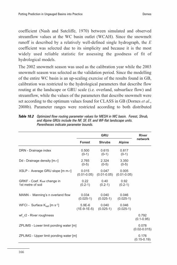
coefficient (Nash and Sutcliffe, 1970) between simulated and observedstreamflow values at the WC basin outlet (WCAH). Since the snowmeltrunoff is described by a relatively well-defined single hydrograph, the Ecoefficient was selected due to its simplicity and because it is the mostwidely used reliable statistic for assessing the goodness of fit ofhydrological models. The 2002 snowmelt season was used as the calibration year while the 2003snowmelt season was selected as the validation period. Since the modellingof the entire WC basin is an up-scaling exercise of the results found in GB,calibration was restricted to the hydrological parameters that describe flowrouting at the landscape or GRU scale (i.e. overland, subsurface flow) andstreamflow, while the values of the parameters that describe snowmelt wereset according to the optimum values found for CLASS in GB (Dornes et al.,2008b). Parameter ranges were restricted according to both distributed

166


GRU

Forest Shrubs Alpine

Rivernetwork

DRN - Drainage index 0.500(0-1)

0.615(0-1)

0.817(0-1)

Dd - Drainage density [m ]-1 2.765(0-5)

2.324(0-5)

3.350(0-5)

XSLP - Average GRU slope [m m ]-1 0.015(0.01-0.05)

0.047(0.01-0.05)

0.005(0.01-0.05)

GRKF - Coef. K change in1st metre of soil

sat 0.22(0.2-1)

0.40(0.2-1)

0.92(0.2-1)

MANN - Manning’s n overland flow 0.034(0.025-1)

0.040(0.025-1)

0.046(0.025-1)

WFCI - Surface K [m s ]sat-1 5.9E-6

(1E-9-1E-5)0.040

(0.025-1)0.046

(0.025-1)

wf_r2 - River roughness 0.792(0.1-0.95)

ZPLIMS - Lower limit ponding water [m] 0.078(0.02-0.015)

ZPLIMG - Upper limit ponding water [m] 0.176(0.15-0.19)

Table 10.2 Optimized flow routing parameter values for MESH in WC basin. Forest, Shrub,and Alpine GRUs include the NF, SF, EF, and WF-flat landscape units.Parentheses indicate parameter bounds.

observations at GB (e.g., McCartney et al., 2006; Bewley et al., 2007) andprior information (e.g., Verseghy et al., 1993; Davison et al., 2006) forsimilar environments. Figure 10.3 shows the CLASS landscape basedsimulations of the snowcover ablation when distributed and solar forcingand initial conditions are considered. Forest parameters not included in thesimulations of GB were set to the default values used in the GlobalEnvironmental Multi-scale (GEM) model of Environment Canada. Calibration was constrained by assigning the same parameter value to all GRUswithin each main vegetation cover. For example, NF slope, SF slope, EF slope,and WF slope and flat landscape units in the shrub area each shared the sameparameterization. Similar approaches were applied in the alpine and forest area.Table 10.2 illustrates the parameters values defined using the DDS algorithm.

167


Figure 10.3 Observed and simulated landscape SWE values with CLASS in Granger Basin(GB) using distributed initial conditions (SWE) and incoming short-wave radiation(K↓). Cal. and Val: calibrated and validated simulations. NF and SF: north andsouth facing slopes, VB: valley bottom, UB: upper basin, PLT: plateau area.(Adapted from Dornes et al., 2008b)

10.6 MODELLING RESULTS

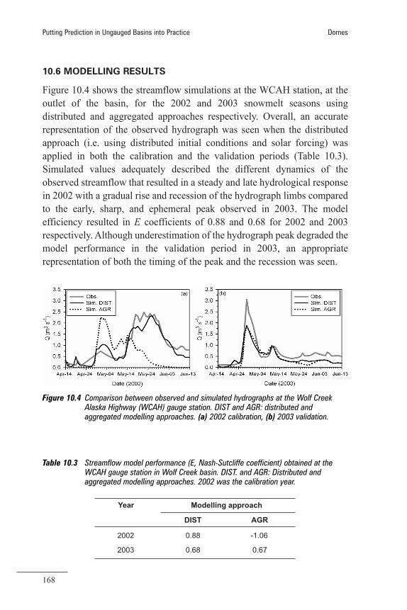
Figure 10.4 shows the streamflow simulations at the WCAH station, at theoutlet of the basin, for the 2002 and 2003 snowmelt seasons usingdistributed and aggregated approaches respectively. Overall, an accuraterepresentation of the observed hydrograph was seen when the distributedapproach (i.e. using distributed initial conditions and solar forcing) wasapplied in both the calibration and the validation periods (Table 10.3).Simulated values adequately described the different dynamics of theobserved streamflow that resulted in a steady and late hydrological responsein 2002 with a gradual rise and recession of the hydrograph limbs comparedto the early, sharp, and ephemeral peak observed in 2003. The modelefficiency resulted in E coefficients of 0.88 and 0.68 for 2002 and 2003respectively. Although underestimation of the hydrograph peak degraded themodel performance in the validation period in 2003, an appropriaterepresentation of both the timing of the peak and the recession was seen.

168


Figure 10.4 Comparison between observed and simulated hydrographs at the Wolf CreekAlaska Highway (WCAH) gauge station. DIST and AGR: distributed andaggregated modelling approaches. (a) 2002 calibration, (b) 2003 validation.

Modelling approachYear

DIST AGR

2002 0.88 -1.06

2003 0.68 0.67

Table 10.3 Streamflow model performance (E, Nash-Sutcliffe coefficient) obtained at theWCAH gauge station in Wolf Creek basin. DIST. and AGR: Distributed andaggregated modelling approaches. 2002 was the calibration year.

Conversely, when the aggregated approach was applied by assuming abasin-wide average initial snowcover and uniform (i.e. over horizontalterrain) incoming solar radiation, the model performance was drasticallydegraded in 2002 with a less noticeable effect in 2003 compared to thedistributed approach. To avoid the possible influence of calibration in thecomparison between distributed and aggregated approaches, simulationsusing the aggregated approach were also calibrated in 2002 using the DDSalgorithm. The inappropriate prediction of the observed hydrograph thatresulted in a negative E coefficient highlighted the importance ofconsidering the spatial distribution of initial conditions and solar forcing inmodel performance.Reasons that might explain the different model performance from using bothdistributed and aggregated approaches can be found by analyzing the basinstreamflow response. Typically, the streamflow response of the WC basin iscontrolled by sequential melt timing between the different ecosystems and bythe shrub tundra zone due to its larger extent, central location, and deepersnow packs compared to the forest and alpine areas. Melt starts around themiddle of April in the forest area, followed by the shrub tundra zone with anonset of melt around April 20, whereas melt in the alpine area starts aroundthe end of April. Furthermore, streamflow dynamics can by affected by warmair advection over the melting snowcover, enhancing melt, and acceleratingstreamflow response. A combination of these processes can lead tosynchronized or unsynchronized melt events between the different landscapesresulting in different basin streamflow responses. For the 2002 snowmeltseason, the onset of melt was rather late and driven by increases in both airtemperature and incident solar radiation. These atmospheric factors, combinedwith large snowdrifts observed on NF slopes, resulted in a late and single peakstreamflow response. The aggregated model using a basin average initial SWEand incoming solar radiation not corrected by topography, simulated meltsearlier than occurred. The 2003 snowmelt season showed an onset of melt asa consequence of above freezing air temperatures earlier in the season thatstopped as the temperatures fell below the freezing point on May 2 (Figure10.5). This phenomenon generated a sharp and early streamflow response.Later in the season, the increasing air temperatures and solar radiationcombined with lower amounts of initial snow on the NF slopes andcomparatively larger snowcovers on the SF slopes resulted in a steadystreamflow response. Simulations using the aggregated approach at the basin

169


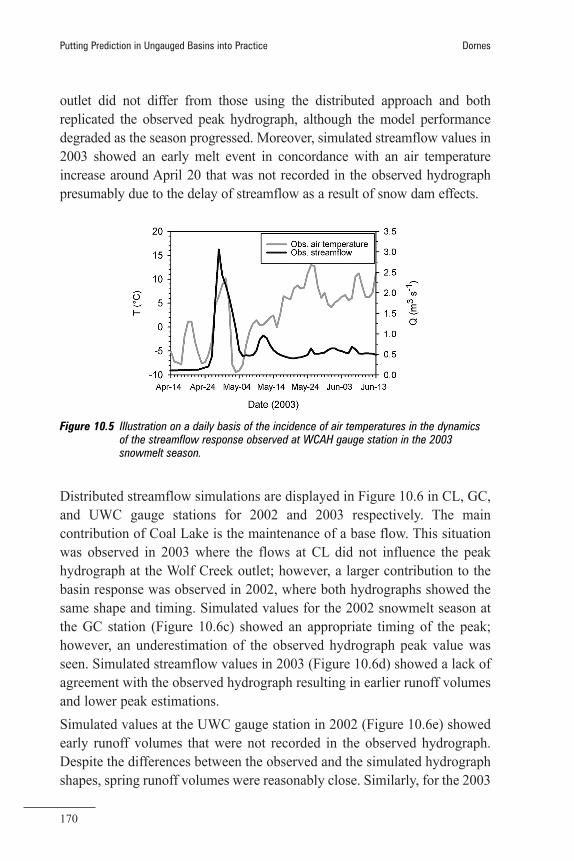
outlet did not differ from those using the distributed approach and bothreplicated the observed peak hydrograph, although the model performancedegraded as the season progressed. Moreover, simulated streamflow values in2003 showed an early melt event in concordance with an air temperatureincrease around April 20 that was not recorded in the observed hydrographpresumably due to the delay of streamflow as a result of snow dam effects.

Distributed streamflow simulations are displayed in Figure 10.6 in CL, GC,and UWC gauge stations for 2002 and 2003 respectively. The maincontribution of Coal Lake is the maintenance of a base flow. This situationwas observed in 2003 where the flows at CL did not influence the peakhydrograph at the Wolf Creek outlet; however, a larger contribution to thebasin response was observed in 2002, where both hydrographs showed thesame shape and timing. Simulated values for the 2002 snowmelt season atthe GC station (Figure 10.6c) showed an appropriate timing of the peak;however, an underestimation of the observed hydrograph peak value wasseen. Simulated streamflow values in 2003 (Figure 10.6d) showed a lack ofagreement with the observed hydrograph resulting in earlier runoff volumesand lower peak estimations.Simulated values at the UWC gauge station in 2002 (Figure 10.6e) showedearly runoff volumes that were not recorded in the observed hydrograph.Despite the differences between the observed and the simulated hydrographshapes, spring runoff volumes were reasonably close. Similarly, for the 2003

170


Figure 10.5 Illustration on a daily basis of the incidence of air temperatures in the dynamicsof the streamflow response observed at WCAH gauge station in the 2003snowmelt season.

snowmelt season, simulated values showed an earlier snowmelt runoffresponse (Figure 10.6f). Overall, differences between distributed simulatedand observed streamflow values illustrate that the model with the givenspatial resolution is not able to accurately replicate the complexity of small-scale snowmelt runoff processes. Good agreement of simulated andobserved runoff volumes and less important differences in replicating therunoff dynamics were seen in 2002 when the snowmelt runoff response wascharacterized by a single peak event. Larger differences in describing boththe observed dynamics and runoff volumes were observed in 2003 as a resultof the complex runoff response that resulted in lower flows and multi-peak

171


Figure 10.6 Comparison between observed and validated simulated hydrographs. (a) and (b)at the Coal Lake (CL) gauge station (drainage area: 71 km2), (c) and (d) at theGranger Creek (GC) gauge station (drainage area: 6 km2), and (e) and (f) at theUpper Wolf Creek (UWC) gauge station (drainage area: 15 km2) for 2002 and2003 respectively within each pair.

hydrographs. The inherent observation errors of low flow volumes, and theinaccessibility of the gauge stations early in the melt season, could alsocontribute to observational uncertainty.Distributed simulated values of snowcover depletion were extracted in thoseplaces where distributed observations were available. Figure 10.7 illustratesthe comparison between simulated snowcover depletion values with snowpillow observations at the BB station for 2002 and 2003 and with snow surveyvalues measured at the F station in 2003. Evaluation of the model performanceagainst snow pillow data was conducted by comparing the simulations againstthe 5-day average of the observational data. Overall, there is reasonableagreement between simulations of the snowcover depletion and observedsnowcover values for both years (Figures 10.7a and b), particularly since thesnow pillow data represents the melting of an unvegetated snow pack.Differences were more evident in 2003, where the model results were nottotally able to describe the observed fast depletion of the snow pack. In theforested area (Figure 10.7c), an adequate description of the early stages ofmelt was seen despite the sparse data through the snowmelt period.

Limitations to this approach were i) coarse scale of modelling compared tosmall sub-basins with stream gauges in WC prevented small scale validationof the model, ii) non-physical snowcover depletion and vegetationparameters were present that could not be related to field observations, andiii) calibration of shrub and vegetation parameters may have masked effectsof shrub emergence, small-scale advection, and micrometeorologicaldifferences between tiles. There needs to be further assessment of whetherto include these in the model.

172


Figure 10.7 Comparison between observed and validated simulated snowcover depletion.(a) and (b) Buck-brush (BB) site (snow pillow data), and (c) Forest (F) site (snowsurvey data).

10.7 CONCLUSIONS

This study illustrates an example of a new approach for physically basedmodelling of snowcover ablation and snowmelt runoff in complex subarcticenvironments with limited data while retaining integrity in the processrepresentations. This modelling methodology is based on the combination ofinductive and deductive reasoning approaches. The inductive (i.e. top-down) modelling approach, based on a basin-wide understanding gainedfrom observations of the main factors that drive the snowmelt processes innorthern mountainous areas, was used for representing the landscapeheterogeneity, hence the spatial model representation was based onlandscape units. The deductive (i.e. bottom-up) modelling approach wasapplied for detailed process descriptions that incorporated physically basedalgorithms with a priori parameter sets describing snowmelt. Thephilosophical basis of the modelling approach is the desire to describe theprocesses in as physically realistic a manner as possible, given theavailability of data and parameters to run the model.

Simulated streamflow values using distributed initial conditions ofsnowcover and incoming solar forcing were able to describe the differenttiming and magnitude of the basin responses observed in both of the studyyears. When the aggregated approach was applied, the model was unable tosimulate the dynamics of the basin streamflow in 2002 when the runoffresponse was largely governed by solar radiation and the negativeassociation between snow accumulation and melt energy observed in theshrub tundra area. Conversely, the differences between the distributed andaggregated approaches were less important when temperature was a keyfactor as in the onset of melt in 2003. Melt synchronicity was reduced withgreater incoming short-wave radiation, so the more clear skies prevailed, thegreater the duration of melt over the basin. The distributed modellingapproach was able to properly describe the sequential melt timing, whereasthe aggregated approach failed. Under conditions with greater cloudy skies,both modelling approaches had a very similar performance as a result of aless important effect of the initial conditions and solar forcing on the onsetof melt.

The selection of landscape units defined according to premelt snowcoverconditions, vegetation cover, and topographic characteristics appears to bean effective method to reduce the size of the parameter sets and still retain

173


physical consistency. These model units can be viewed as signatures ofhydrological variability or predictor variables (Sivapalan et al., 2003b;Sivapalan, 2005) which have a significant importance for accuratepredictions in northern and mountain basins typically characterized asungauged or poorly gauged basins and for land surface-atmosphericinteractions at both small and larger scales.

174


Documents

HOW TO COMBINE INDUCTIVE AND DEDUCTIVE APPROACHES … · HOW TO COMBINE INDUCTIVE AND DEDUCTIVE APPROACHES TO PREDICTION? Pablo F. Dornes1,2 1Centre for Hydrology, University of Saskatchewan,