Embed Size (px)
Citation preview
Household Occupancy Monitoring Using Electricity MetersWilhelm Kleiminger
Dept. of Computer ScienceETH Zurich, Switzerland
Christian BeckelDept. of Computer ScienceETH Zurich, Switzerland
Silvia SantiniEmbedded Systems LabTU Dresden, Germany
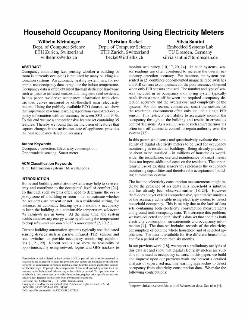
ABSTRACTOccupancy monitoring (i.e. sensing whether a building orroom is currently occupied) is required by many building au-tomation systems. An automatic heating system may, for ex-ample, use occupancy data to regulate the indoor temperature.Occupancy data is often obtained through dedicated hardwaresuch as passive infrared sensors and magnetic reed switches.In this paper, we derive occupancy information from elec-tric load curves measured by off-the-shelf smart electricitymeters. Using the publicly available ECO dataset, we showthat supervised machine learning algorithms can extract occu-pancy information with an accuracy between 83% and 94%.To this end we use a comprehensive feature set containing 35features. Thereby we found that the inclusion of features thatcapture changes in the activation state of appliances providesthe best occupancy detection accuracy.
Author KeywordsOccupancy detection; Electricity consumption;Opportunistic sensing; Smart meter.
ACM Classification KeywordsH.m. Information systems: Miscellaneous.
INTRODUCTIONHome and building automation systems may help to save en-ergy and contribute to the occupants’ level of comfort [24].To this end, such systems often need to determine the occu-pancy state of a building or room – i.e. to estimate whetherthe residents are present or not. In a residential setting, forinstance, an automatic heating system monitors occupancyto keep the building at a comfortable temperature wheneverthe residents are at home. At the same time, the systemavoids unnecessary energy waste by allowing the temperatureto drop whenever the household is unoccupied [2, 20, 21].
Current building automation systems typically use dedicatedsensing devices such as passive infrared (PIR) sensors andreed switches to provide occupancy monitoring capabili-ties [1, 21, 29]. Recent results also show the feasibility ofopportunistically using network logins and GPS trackers to
Permission to make digital or hard copies of all or part of this work for personal orclassroom use is granted without fee provided that copies are not made or distributedfor profit or commercial advantage and that copies bear this notice and the full citationon the first page. Copyrights for components of this work owned by others than theauthor(s) must be honored. Abstracting with credit is permitted. To copy otherwise, orrepublish, to post on servers or to redistribute to lists, requires prior specific permissionand/or a fee. Request permissions from [email protected] ’15, September 07 - 11, 2015, Osaka, JapanCopyright is held by the owner/author(s). Publication rights licensed to ACM.ACM 978-1-4503-3574-4/15/09...$15.00DOI: http://dx.doi.org/10.1145/2750858.2807538
monitor occupancy [10, 17, 20, 24]. In such systems, sen-sor readings are often combined to increase the overall oc-cupancy detection accuracy. For instance, the system pre-sented in [2] combines door-mounted magnetic reed switchesand PIR sensors to compensate for the poor accuracy obtainedwhen only PIR sensors are used. The number and type of sen-sors included in an occupancy monitoring system typicallyresult from a trade-off between the required occupancy de-tection accuracy and the overall cost and complexity of thesystem. For this reason, commercial smart thermostats forthe residential environment often only include a single PIRsensor. This restricts their ability to accurately monitor theoccupancy throughout the building and results in erroneouscontrol decisions. As a result, users of such smart thermostatsoften turn off automatic control to regain authority over thesystem [32].
In this paper, we discuss and quantitatively evaluate the suit-ability of digital electricity meters to be used for occupancymonitoring in residential buildings. Being already present –or about to be installed – in millions of households world-wide, the installation, use and maintenance of smart metersdoes not impose additional costs on the residents. The oppor-tunistic use of existing sensors thus increases the occupancymonitoring capabilities and therefore the acceptance of build-ing automation systems.
The fact that electricity consumption measurements might in-dicate the presence of residents in a household is intuitiveand has already been observed earlier [18, 23]. Howeverthere does not yet exist a comprehensive, quantitative analysisof the accuracy achievable using electricity meters to detecthousehold occupancy. This is mainly due to the lack of datasets containing both electricity consumption measurementsand ground truth occupancy data. To overcome this problem,we have collected and published1 a data set that contains bothelectricity consumption measurements and occupancy infor-mation [4]. The data set includes records of the electricityconsumption of both the whole household and of selected ap-pliances. The data is available for five different householdsand for a period of more than six months.
In our previous work [18], we report a preliminary analysis ofthis data set and show that digital electricity meters are suit-able to be used as occupancy sensors. In this paper, we buildand improve upon our previous work and present a detailedanalysis of supervised machine learning approaches to detectoccupancy from electricity consumption data. We make thefollowing contributions:
1http://vs.inf.ethz.ch/res/show.html?what=eco-data. See also [4].

• Exhaustive analysis of the feature space: To investi-gate which characteristics of the load curve best revealoccupancy, we extend the feature set of our preliminarywork [18] from 10 to 35 features. To deal with the ex-tended feature set, we employ dimensionality reduction, inparticular principal component analysis (PCA) and featureselection. We show that features capturing appliance statechanges are best suited for occupancy detection.
• Improved classification performance: We consider a setof seven classifiers (instead of 4 in our previous work) andshow that the enlarged feature space in conjunction withdimensionality reduction achieves classification accuraciesup to 94%.
• Feasibility analysis with regards to smart heating: Byanalysing the ability of our approach to monitor occupancytransitions, we evaluate the feasibility of using digital elec-tricity meters to provide occupancy data for controlling asmart thermostat.
RELATED WORKThe approaches most related to our work can be found inthe fields of building occupancy detection, nonintrusive loadmonitoring and analysis of electricity consumption data.
Building occupancy detectionSeveral authors have focussed on the design, deploymentand evaluation of approaches to detect occupancy both incommercial and residential buildings. A good overview ofexisting approaches for occupancy detection is provided byNguyen and Aiello [24]. One observation made by the au-thors is that only a small fraction of the approaches presentedin the literature have been evaluated in real deployments. Theauthors thus stress “a vital need” to verify conceptual resultsin “real-life installations” [24]. Recent work shows resultsfrom such real-life deployments [1, 7, 8, 21].
However, most occupancy monitoring systems require ded-icated hardware and are evaluated over a short time horizononly. While some authors combine PIR sensors with reedswitches [1, 21, 29], several authors have also combined PIRsensors with call monitoring [7] or microphones [25], whileanother solution requires dedicated camera networks [8].Lu et al. instrumented eight homes with PIR sensors andreed switches for a duration varying from one to twoweeks depending on the household. In a similar approach,Agarwal et al. describe the control of a heating, ventilationand cooling (HVAC) system in a university building [1].These approaches are similar to our work because theyinvestigate and quantitatively evaluate the use of specificsensors to detect occupancy. However, instead of relying ona dedicated infrastructure, we explore the possibility of usingoff-the-shelf digital electricity meters – which are becomingmandatory in many countries [26] – to reduce the need foradditional hardware. Furthermore, our analysis relies ondata collected over significantly longer periods of time thanprevious work.
Nonintrusive load monitoring (NILM)A number of authors have looked into so-called nonintrusiveload monitoring (NILM) approaches to infer the disaggre-gated (i.e. device-level) electricity consumption from aggre-gate data. NILM is closely related to our approach as theactivation state of home appliances may give an indicationof the current activity of the occupants and thus the build-ings occupancy. Froehlich et al. provide an overview of thesetechniques in [9].
Early NILM research was led by George Hart, who useddevice signatures based on step changes in the electricityconsumption to detect individual appliances [12]. However,follow-up work has shown that current algorithms are onlyable to reliably detect a few appliances (e.g. cooling appli-ances or the washing machine) when the electricity consump-tion is sampled at a granularity of 1 Hz [4]. Our results showthat these appliances are not suitable for occupancy monitor-ing as their operation exhibits a low correlation with occu-pancy.
More recent approaches make use of transient [27] or con-tinuous [11] electrical noise on the power line to detect theactivation state of appliances. However, like the approachby Hart, these require additional instrumentation and train-ing. Froehlich et al. note that the calibration requires usersto “walk around the home, activating and deactivating eachdevice or appliance at least once” [9].
In contrast to most NILM approaches, our system only re-quires the annotation of the occupancy state of the household.While asking the user to supply these annotations is still bur-densome, the effort is small when compared to calibrating allappliances. In addition, the effort can be significantly reducedby running a simple heuristic unsupervised occupancy detec-tion (e.g. by comparing the current electricity consumption tothe mean of the nighttime consumption) and proposing pos-sible ground truth occupancy schedules to the user.
Occupancy and the electric load curveIn [23], Molina-Markham et al. suggest that household ac-tivities can be inferred from aggregate electricity consump-tion data. They collected data at 1Hz from three homes overtwo months and let occupants annotate which appliances theyhave used at what time. The authors observed that there aredifferences in the consumption data depending on whetherthe occupants are present or absent. However, this observa-tion is based on visual inspection of the electric load curves.No quantitative analysis of the possibility of using aggre-gate electricity consumption data to automatically detect oc-cupancy is provided.
In a recent workshop publication we presented the results ofa preliminary analysis of an occupancy monitoring infras-tructure relying on electricity consumption data [18]. At thesame workshop, Chen et al. discussed the potential of digi-tal electricity meters to be used for performing non-intrusiveoccupancy monitoring [6]. In particular, they presented athreshold-based method to detect occupancy from aggregateelectricity consumption data. The authors evaluated theirmethod using data collected in two homes over a summer

week. We build upon this and our previous work by consid-ering a large set of features including those used by Chen etal. and base our analysis on a data set collected in five homesand over a period of more than six months. While in [18] wefocussed on the description of the data set and the presenta-tion of preliminary, encouraging results, this paper presentsa more detailed analysis of the potential of common digitalelectricity meters to be used as occupancy sensors.
Other authors utilise device-level information to monitoroccupancy. Ming et al. suggest a zero-training algorithmbased on rough estimates of the participants’ working sched-ules [16]. Their so-called “PresenceSense” approach es-timates occupancy in an office environment using the av-erage power, standard deviation and absolute maximumpower change of individual appliances measured by ACmenodes [15]. In contrast to PresenceSense, our work requiresonly the installation of a single digital electricity meter andfocusses on residential buildings.
ECO DATA SETFor our analysis we use the publicly available Electricity Con-sumption and Occupancy (ECO) data set. To the best of ourknowledge, this data set is the largest one containing bothelectricity consumption data and ground truth occupancy in-formation2. We have collected this data in the period fromJune 2012 to January 2013 – for a total of more than sixmonths – in five Swiss households. The characteristics of thehouseholds (number of occupants, type of household, etc.)are described in [18] and [4]. We refer to the households asr1, r2, etc. to preserve their anonymity (we use the samenumbering as in [18]).
The samples of electricity consumption have been collectedevery second using off-the-shelf digital electricity meters in-stalled in the households. One sample represents the averagepower (in watts) consumed by the household during the sec-ond preceding the measurement. We refer to these recordsas the aggregate electricity consumption as they refer to theconsumption of the whole household.
Fine-grained occupancy data is available for two periods, re-ferred to as summer (July to September 2012) and winter(November 2012 to January 2013). Before using this datafor our analysis, we perform the same pre-processing stepsdescribed in [18] to eliminate erroneous ground truth data.After this data cleaning phase, the number of days for whichground truth data is available for households r1, r2, r3, r4 andr5 are 39, 83, 57, 38 and 43 for the summer period; and 46,45, 21, 48 and 31 for the winter period, respectively.
SYSTEM DESIGNIn residential buildings, a change in the overall electricityconsumption often provides an indication of occupancy asmany appliances are used to increase comfort and/or to re-place manual labour. Figure 1 shows the electricity consump-tion of a representative day for household r2 and the output ofa simple thresholding classifier. The latter assumes the house-hold to be occupied whenever the current power is higher than2Ground truth occupancy data has been entered manually by the res-idents using tablet computers mounted near the main entrance.
0
500
1000
1500
2000
2500
3000
Tota
lpow
er(W
)
Occupied Unoccupied Occupied
00:00 03:00 06:00 09:00 12:00 15:00 18:00 21:00Time of day
unocc.
occ.
Figure 1: Example of an occupancy detection algorithmbased on mean thresholding.
the 24-hour mean. The performance of this classifier showsthat even a primitive strategy may detect occupancy. In thispaper, we build upon this observation by analysing how elec-tric load curves can be used to monitor occupancy.
Deriving features from the electric load curveIn order to infer occupancy from the raw electricity consump-tion data, we identify features of the electric load curve thatare indicative of occupancy. A good indication of occupancyare appliance state changes triggered by the interaction ofan occupant (e.g. an occupant turning on the television orstove) [23]. For this reason, we focus on identifying featuresthat relate to the operation of occupancy-relevant appliancesand allow to directly infer occupancy from the aggregate elec-tricity consumption.
In order to identify such features, we compare the day-time3
(6 a.m. to 10 p.m.) electricity consumption during occupiedperiods to times when the household is unoccupied.
Table 1 summarises the selected features. All features arecomputed at 15-minute intervals. Every day is representedas a sequence of Ns time slots of length Ts. As the aggregateelectricity consumption is sampled at 1Hz, the interval lengthof Ns = 15 means that each feature is computed on a 900-element vector (i.e. Ts = 900). All features listed in Table 1– apart from pprob, pfixed and ptime – are computed sep-arately for each phase and the sum of all three phases. Thesubscripts 1, 2 or 3 are used to indicate that a feature hasbeen computed on the data corresponding to phase 1, 2 or 3,respectively. Likewise, the subscript 123 indicates a featurecomputed on the combined consumption of all three phases.In summary, we consider the features min, max, mean, std,sad, cor1, onoff, range, pprob, pfixed and ptime com-puted on the three electrical phases. Using these features weaim to capture both the absolute value as well as the variabil-ity of the electricity consumption.
Absolute value of the power consumptionThe min, max and mean features denote the minimum, max-imum and arithmetic average of each slot.
3The ECO data set does not contain ground truth data on sleepingpatterns, we thus leave the detection of sleep for future work.

Table 1: Features computed on the aggregate electricity consumption traces.
# Feature names Descriptionf1, f2, f3 min1, min2, min3 Minimum of the samples for phase 1, 2 and 3f4 min123 Minimum of the samples for the sum of phase 1, 2 and 3f5, f6, f7 max1, max2, max3 Maximum of the samples for phase 1, 2 and 3f8 max123 Maximum of the samples for the sum of phase 1, 2 and 3f9, f10, f11 mean1, mean2, mean3 Arithmetic average of the samples for phase 1, 2 and 3f12 mean123 Arithmetic average of the samples for the sum of phase 1, 2 and 3f13, f14, f15 std1, std2, std3 Standard deviation of the samples for phase 1, 2 and 3f16 std123 Standard deviation of the samples for the sum of phase 1, 2 and 3f17, f18, f19 sad1, sad2, sad3 Sum of absolute differences of the samples for phase 1, 2 and 3f20 sad123 Sum of absolute differences of the samples for the sum of phase 1, 2 and 3f21, f22, f23 cor11, cor12, cor13 Autocorrelation at lag 1 computed over the samples for phase 1, 2 and 3f24 cor1123 Autocorrelation at lag 1 computed over the samples for the sum of phase 1, 2 and 3f25, f26, f27 onoff1, onoff2, onoff3 Number of detected on/off events for phase 1, 2 and 3f28 onoff123 Number of detected on/off events for the sum of phase 1, 2 and 3f29, f30, f31 range1, range2, range3 Range of the samples for phase 1, 2 and 3f32 range123 Range of the samples for the sum of phase 1, 2 and 3f33 pprob Empirical probability of the slot to be occupiedf34 pfixed 1 (occupied) from 9 a.m. to 5 p.m., 0 (unoccupied) otherwisef35 ptime Slot number (i.e. 1 – 65)
Variability of the power consumptionA high variability in the electricity consumption may pro-vide an indicator of human activity. Significant changes inthe power consumption are often the result of human actions(e.g. by operating the stove) or the operation of applianceswith varying consumption levels (e.g. a television set withLED backlight). We chose the std (standard deviation), sad(sum of absolute differences), cor1 (autocorrelation at lagone) and onoff4 features as indicators of such variability.
Temporal dependence of occupancyAs building occupancy is also dependent upon the currenttime of the day, we use the pprob, pfixed and ptime featuresto model the temporal aspects of occupancy. pprob is the em-pirical prior probability of a 15-minute slot to be occupied.pprob is computed from the ground truth occupancy data. Tothis end, only data from the training set is used. pfixed is a“dummy” prior probability that assumes the household to bealways unoccupied between 9 a.m. and 5 p.m. on weekdaysand to be always occupied on weekends. ptime is the num-ber of the current slot and thus directly introduces a notionof time. Slots are numbered from 1 to 65, with the first slotcorresponding to the period between 6 a.m. and 6:15 a.m. andthe last one to the time between 10 p.m. and 10:15 p.m.
ClassifiersIn order to use a building’s electricity consumption to moni-tor occupancy one requires a mapping from the feature space(e.g. a mean consumption of 100W) to occupancy classes(i.e. [feature] → {home, away}). In supervised ma-chine learning, this mapping function – the classifier – is in-ferred from labelled training data. The training data is used to
4On/off events occur when an appliance is switched on or off. Wedetect these events using a simple heuristic: If the difference be-tween a sample and its predecessor is bigger than a threshold ThAand this difference remains higher than ThA for at least ThT seconds,an on/off event is detected. We set ThA = 30W and ThT = 30 s.
iteratively refine the classifier to maximise the number of ex-amples (i.e. [[feature], class] tuples) correctly as-signed by the classifier. To make sure that the classifier isnot overfitting the data (i.e. it does capture the underlying re-lationship between features and classes rather than the noisein the data), we divide the data into training and test sets.Thereby, the test set provides an unbiased test of the perfor-mance of the classifier on previously unseen data. A numberof learning algorithms to build classifiers have been suggestedin the literature. The learning algorithms used in this paperare support vector machines (SVMs), K-nearest neighbours(KNNs), Gaussian mixture models (GMMs), hidden Markovmodels (HMMs) and a simple thresholding (THR) approach.
SVMs are widely-used supervised learning models and algo-rithms that perform linear and non-linear classification. Forthe implementation of the SVM classifier we employed theLIBSVM library by Chang and Lin [5].
A KNN is a non-parametric model for classification whichclassifies an example using a majority vote on the classesof its k most similar neighbours. This means it doesnot require an explicit learning phase. We used theClassificationKNN classes from the Matlab StatisticsToolbox to implement our KNN classifier. We empiricallydetermined k = 1 and use the Euclidean distance measure toobtain the nearest neighbours.
The limited size of the ECO data set prohibits us from build-ing empirical multivariate probability density functions for acombination of all features. To alleviate this problem, weuse GMMs, which allow to approximate these by a weightedsum of individual Gaussian component distributions [28].The GMMs are built by iteratively refining the parametersof its k Gaussian component distributions to fit the inputdata. To avoid overfitting, we chose a suitable k by min-imising the Akaike information criterion (AIC) [3]. TheAIC penalises a larger number of components while reward-ing goodness of fit. For the implementation we chose thegmdistribution class from the Matlab Statistics Tool-
box. The training data is used to create GMMs for both theoccupied an unoccupied distribution. The classification of un-known data is performed by maximum-likelihood (i.e. com-paring the likelihood of the sample belonging to either distri-bution).
The hitherto presented classifiers are stateless – i.e. they donot take into account the previous occupancy state. Occu-pancy, however, is stateful. In fact, during any particular 15-minute interval a household is most likely to stay in its currentstate. An occupancy monitoring system should thus focuson detecting occupancy transitions (from occupied to unoccu-pied and vice versa). To investigate such a stateful occupancymonitoring system, we use a HMM classifier which relatesits hidden states (i.e. occupied, unoccupied) to emissions (i.e.the observed features of the electricity consumption) usingmatrices of emission and transition probabilities. The transi-tion matrix contains the probability of staying in or movingout of any state for all states. To obtain the matrix of emissionprobabilities we first construct a 2-dimensional GMM of thefirst principal component and the ptime feature (i.e. the slotnumber) for both the occupied and unoccupied states, respec-tively. The discrete emission probabilities are then obtainedby numerally evaluating the integral of the GMMs over a ma-trix of 30× 16 bins.
From Figure 1 we conjecture that a high electricity consump-tion may have a positive correlation with occupancy. To in-vestigate whether a simple classifier may use this correlation,we implemented the THR classifier which computes the meanfor each feature vector during all unoccupied times. It thenuses these means as thresholds to label a feature as occupied.To obtain the final classification, the THR classifier computesa majority vote over all features of a particular interval.
Dimensionality reductionThe 35 features introduced in Table 1 allow us to capture var-ious characteristics of the electric load curve. However, whilesome classifiers may utilise the full feature set, others performbest on a subset of these features. Indeed, for each classifierthere exists an optimal subset of features that maximises itsperformance [30]. To find these subsets and to limit the fea-tures to the most descriptive ones, we used sequential forwardselection (SFS) and principal component analysis (PCA).
Feature selectionThe optimal set of features may be found by performinga brute-force evaluation of all possible combinations [30].Alas, the complexity of such an exhaustive search grows ex-ponentially with the number of features. In this paper, weconsider the sequential forward selection (SFS) [30] algo-rithm to heuristically identify reasonable subsets of features.
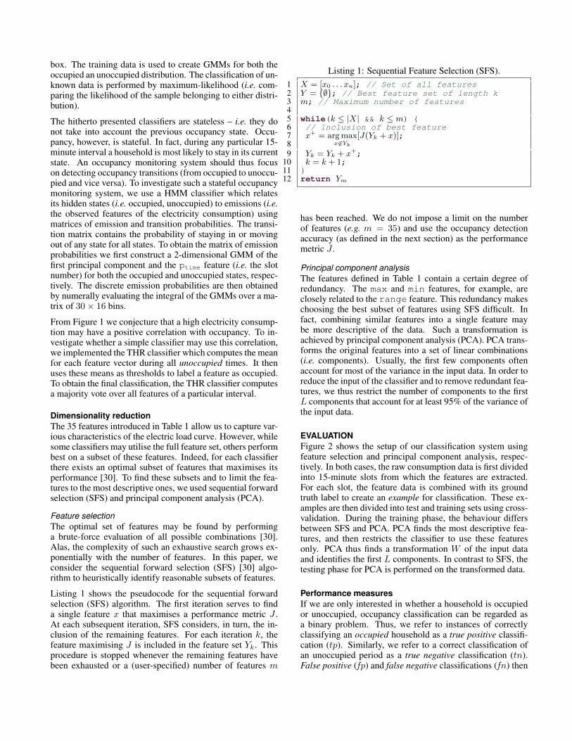
Listing 1 shows the pseudocode for the sequential forwardselection (SFS) algorithm. The first iteration serves to finda single feature x that maximises a performance metric J .At each subsequent iteration, SFS considers, in turn, the in-clusion of the remaining features. For each iteration k, thefeature maximising J is included in the feature set Yk. Thisprocedure is stopped whenever the remaining features havebeen exhausted or a (user-specified) number of features m
Listing 1: Sequential Feature Selection (SFS).1 X = [x0 . . . xn]; // Set of all features2 Y = {∅}; // Best feature set of length k3 m; // Maximum number of features45 while(k ≤ |X| && k ≤ m) {6 // Inclusion of best feature7 x+ = argmax
x 6∈Yk
[J(Yk + x)];89 Yk = Yk + x+;
10 k = k + 1;11 }12 return Ym
has been reached. We do not impose a limit on the numberof features (e.g. m = 35) and use the occupancy detectionaccuracy (as defined in the next section) as the performancemetric J .
Principal component analysisThe features defined in Table 1 contain a certain degree ofredundancy. The max and min features, for example, areclosely related to the range feature. This redundancy makeschoosing the best subset of features using SFS difficult. Infact, combining similar features into a single feature maybe more descriptive of the data. Such a transformation isachieved by principal component analysis (PCA). PCA trans-forms the original features into a set of linear combinations(i.e. components). Usually, the first few components oftenaccount for most of the variance in the input data. In order toreduce the input of the classifier and to remove redundant fea-tures, we thus restrict the number of components to the firstL components that account for at least 95% of the variance ofthe input data.
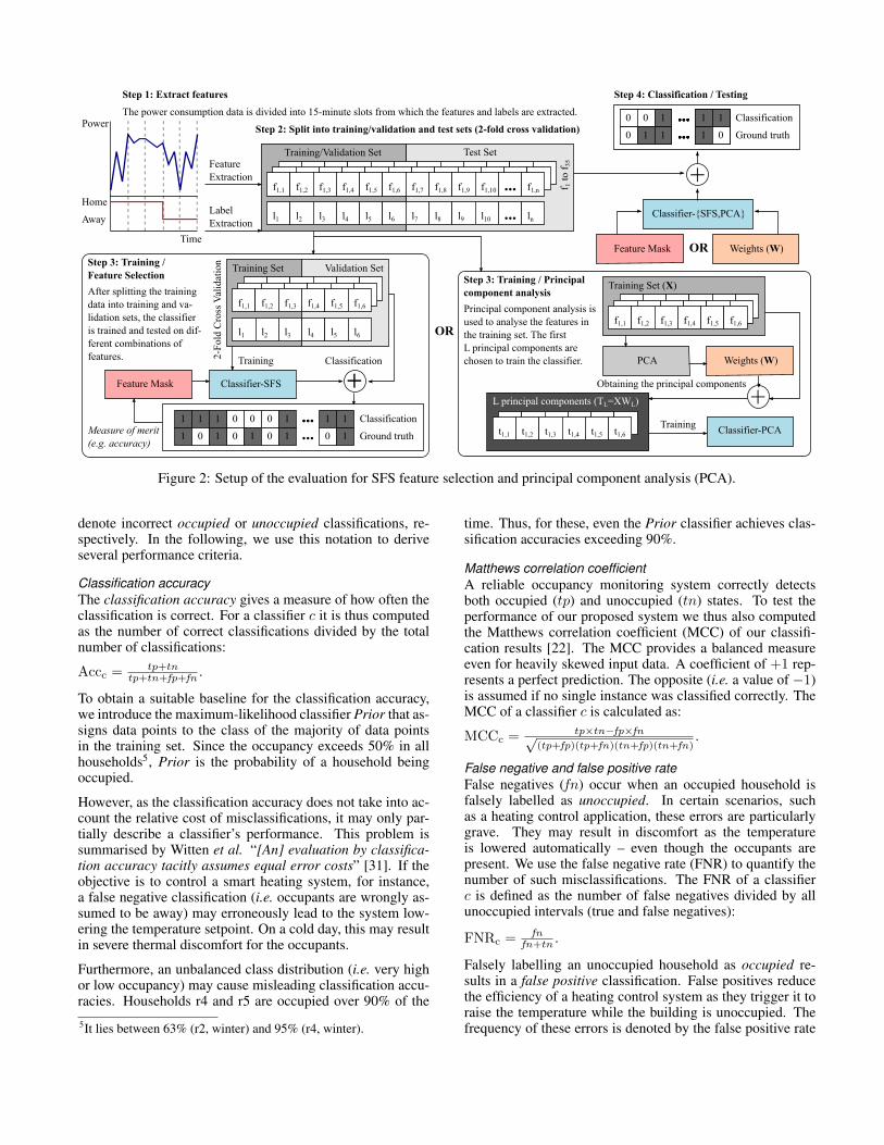
EVALUATIONFigure 2 shows the setup of our classification system usingfeature selection and principal component analysis, respec-tively. In both cases, the raw consumption data is first dividedinto 15-minute slots from which the features are extracted.For each slot, the feature data is combined with its groundtruth label to create an example for classification. These ex-amples are then divided into test and training sets using cross-validation. During the training phase, the behaviour differsbetween SFS and PCA. PCA finds the most descriptive fea-tures, and then restricts the classifier to use these featuresonly. PCA thus finds a transformation W of the input dataand identifies the first L components. In contrast to SFS, thetesting phase for PCA is performed on the transformed data.
Performance measuresIf we are only interested in whether a household is occupiedor unoccupied, occupancy classification can be regarded asa binary problem. Thus, we refer to instances of correctlyclassifying an occupied household as a true positive classifi-cation (tp). Similarly, we refer to a correct classification ofan unoccupied period as a true negative classification (tn).False positive (fp) and false negative classifications (fn) then
FeatureExtraction
Classifier-SFS
Training
+1 01 1 0 0 1 ... 1 1
Classification
Power
Home
Time
Away
f1,1 f1,2 f1,3 f1,4 f1,5
l1 l2 l3 l4 l5LabelExtraction
Training/Validation Set
f1,6 f1,7 f1,8
l6 l7 l8
f1,9 f1,10
l9 l10
f 1 to
f35
f1,n
ln
Test Set
f1,1 f1,2 f1,3 f1,4 f1,5
l1 l2 l3 l4 l5
Training Set
f1,6
l6
Validation Set
Step 2: Split into training/validation and test sets (2-fold cross validation)
2-F
old
Cro
ss V
alid
atio
n
+
Step 3: Training / Feature Selection
Classifier-{SFS,PCA}
Step 4: Classification / Testing
+
Feature Mask
Feature Mask
Step 1: Extract features
After splitting the trainingdata into training and va-lidation sets, the classifier is trained and tested on dif-ferent combinations offeatures.
The power consumption data is divided into 15-minute slots from which the features and labels are extracted.0 0 1 ... 1 1
1 00 1 1 0 1 ... 0 1
0 0 1 ... 1 10 0 1 ... 1 10 0 1 ... 1 1
0 0 1 ... 1 10 0 1 ... 1 10 0 1 ... 1 10 1 1 ... 1 0
Measure of merit(e.g. accuracy)
Classification
Ground truth
Classification
Ground truth
...
...
...
f1,1 f1,2 f1,3 f1,4 f1,5
Training Set (X)
f1,6
Step 3: Training / Principalcomponent analysis
Weights (W)
Principal component analysis isused to analyse the features inthe training set. The firstL principal components arechosen to train the classifier. PCA
t1,1 t1,2 t1,3 t1,4 t1,5
L principal components (TL=XWL)
t1,6 Classifier-PCA
Weights (W)
+Training
Obtaining the principal components
OR
OR
Figure 2: Setup of the evaluation for SFS feature selection and principal component analysis (PCA).
denote incorrect occupied or unoccupied classifications, re-spectively. In the following, we use this notation to deriveseveral performance criteria.
Classification accuracyThe classification accuracy gives a measure of how often theclassification is correct. For a classifier c it is thus computedas the number of correct classifications divided by the totalnumber of classifications:
Accc =tp+tn
tp+tn+fp+fn .
To obtain a suitable baseline for the classification accuracy,we introduce the maximum-likelihood classifier Prior that as-signs data points to the class of the majority of data pointsin the training set. Since the occupancy exceeds 50% in allhouseholds5, Prior is the probability of a household beingoccupied.
However, as the classification accuracy does not take into ac-count the relative cost of misclassifications, it may only par-tially describe a classifier’s performance. This problem issummarised by Witten et al. “[An] evaluation by classifica-tion accuracy tacitly assumes equal error costs” [31]. If theobjective is to control a smart heating system, for instance,a false negative classification (i.e. occupants are wrongly as-sumed to be away) may erroneously lead to the system low-ering the temperature setpoint. On a cold day, this may resultin severe thermal discomfort for the occupants.
Furthermore, an unbalanced class distribution (i.e. very highor low occupancy) may cause misleading classification accu-racies. Households r4 and r5 are occupied over 90% of the
5It lies between 63% (r2, winter) and 95% (r4, winter).
time. Thus, for these, even the Prior classifier achieves clas-sification accuracies exceeding 90%.
Matthews correlation coefficientA reliable occupancy monitoring system correctly detectsboth occupied (tp) and unoccupied (tn) states. To test theperformance of our proposed system we thus also computedthe Matthews correlation coefficient (MCC) of our classifi-cation results [22]. The MCC provides a balanced measureeven for heavily skewed input data. A coefficient of +1 rep-resents a perfect prediction. The opposite (i.e. a value of −1)is assumed if no single instance was classified correctly. TheMCC of a classifier c is calculated as:
MCCc =tp×tn−fp×fn√
(tp+fp)(tp+fn)(tn+fp)(tn+fn).
False negative and false positive rateFalse negatives (fn) occur when an occupied household isfalsely labelled as unoccupied. In certain scenarios, suchas a heating control application, these errors are particularlygrave. They may result in discomfort as the temperatureis lowered automatically – even though the occupants arepresent. We use the false negative rate (FNR) to quantify thenumber of such misclassifications. The FNR of a classifierc is defined as the number of false negatives divided by allunoccupied intervals (true and false negatives):
FNRc =fn
fn+tn .
Falsely labelling an unoccupied household as occupied re-sults in a false positive classification. False positives reducethe efficiency of a heating control system as they trigger it toraise the temperature while the building is unoccupied. Thefrequency of these errors is denoted by the false positive rate

(FPR). The FPR of a classifier c is defined as the number offalse positives divided by all occupied intervals (true and falsepositives):
FPRc =fp
fp+tp .
Cross-validationWe randomly divide the data ten times into different, equi-sized training and testing sets. For each of these runs, thetraining set is used to train the classifiers and the testing setis used to evaluate their performance. Afterwards, the rolesof the sets are switched and the process repeated. So in to-tal, classification is performed 20 times. The two-fold cross-validation tries to avoid that a specific allocation of data intotraining and testing sets creates artefacts in the results. Theuse of ten runs also allows for an assessment of the stability ofthe feature selection6 – i.e. to analyse if different training datayield different feature sets. The overall performance is com-puted as the average of the performance over the 20 roundsof classifications.
Classification limited to daytime hoursDuring the night, the electricity consumption is usually lessindicative of occupancy. Since we also do not have groundtruth data on sleep patterns, we restrict occupancy classifica-tion to the time between 6 a.m. and 10.15 p.m.
Cross validation at day-granularityFor each classification, the HMM classifier requires the previ-ous occupancy state – e.g. at 9.15 a.m. it requires knowledgeabout the occupancy at 9 a.m. To facilitate this, the input datais assigned to training and testing sets at day-granularity.
RESULTSIn this section, we use the features derived from the aggre-gate electricity consumption to quantitatively evaluate the oc-cupancy monitoring performance. We have implemented theSVM, KNN, THR, GMM and HMM classifiers as well as thePrior classifier for baseline comparison. The classifiers es-timate the occupancy state for each time slot from the set offeatures computed on the aggregate electricity consumption.To reduce the dimensionality of the feature space, we evalu-ate the SFS feature selection algorithm and PCA. The usedmethod is indicated by the appendices “-SFS” or “-PCA”,where applicable (e.g. SVM-SFS denotes the usage of theSVM classifier trained using SFS feature selection).
First, we discuss the overall occupancy detection perfor-mance in terms of accuracy, FNR, FPR and MCC. We thenevaluate the performance of the different classifiers and theresults of the feature selection. We conclude this sectionwith discussion on the suitability of monitoring building oc-cupancy using electricity consumption data in a smart heatingscenario.
Overall occupancy detection performanceFor each household, we use C to denote the classifier achiev-ing the highest accuracy (i.e. AccC). To put AccC into con-text, we also evaluate the false positive (FPRC) and false6Feature selection is actually performed using an additional two-fold cross-validation on the training data (cf. Figure 2).
020406080
Household
Perf
orm
ance
a) Summer
AccC FPRAC FNRAC Prior
r1 r2 r3 r4 r50
20406080
Household
Perf
orm
ance
b) Winter
Figure 3: Best accuracy (AccC) and corresponding perfor-mance measures in percent over all classifiers.
negative rates (FNRC) achieved by C. Figure 3 shows theperformance in terms of AccC, FPRC and FNRC for all fivehouseholds in the (a) summer and (b) winter data sets.
In households r1 to r3, the best classifier C outperformsthe Prior accuracy as determined by the maximum-likelihoodclassifier during both summer and winter. The best result isobtained in r2 where AccC is on average 29% higher than thePrior accuracy. Here, the mean accuracy of the summer andwinter periods is 93%. This results, on average, in approx-imately one hour misclassified per day. At the same time,FNRC is 6% on average. Thus, a low fraction of intervalsis misclassified as unoccupied. The average FPRC is 8%,which means that C incorrectly assumes the building to beunoccupied for 38 minutes on average per day.
In households r1 and r3, the best classifiers achieve a ten per-cent improvement over the Prior baseline (AccC = 85% forr1 and AccC = 81% for r3). In contrast to r1, however, theclassifications come with a potential of discomfort caused bytheir false negative rate. In household r1, we observe a FNRof 15%; meaning that 110 minutes are falsely classified asunoccupied while the participants were actually at home. Inhousehold r3, one hour and 35 minutes are misclassified asunoccupied as FNRC = 14%.
In households r4 and r5, the accuracy of the best classifierC does not significantly exceed the performance of the Prior.In contrast to r1 to r4, these two households have very high(i.e. around 90%) occupancy levels. The reasons for the in-ability of the classifiers to outperform the Prior classifier maynot be conclusively established as we lack detailed data onthe behaviour of the occupants. We assume, however, that theresults can in part be explained by the behaviour of the occu-pants. The high occupancy in r4 and r5 means that there maybe periods where a building is occupied while no electricalappliances are in operation. For the classifier, these periodslook identical to those encountered when the building is ac-tually unoccupied. Furthermore, as the buildings are almostalways occupied, the number of such inactive periods is likely

Table 2: Classification accuracy (expressed as percentages)for each household and algorithm in summer and winter.
SFS PCASVM KNN THR SVM KNN GMM HMM Prior
# Summerr1 80 76 77 83 80 78 83 75r2 91 88 76 92 89 76 90 65r3 78 76 71 83 79 70 82 71r4 90 90 85 91 88 70 87 90r5 90 88 81 90 84 59 79 90
Winterr1 82 78 83 84 81 79 87 73r2 93 91 77 94 91 88 92 63r3 70 71 66 78 76 59 71 71r4 92 92 90 92 90 70 84 93r5 82 80 77 85 79 63 74 82
to exceed the occupied periods. This would result in the clas-sifier almost always classifying the home as occupied.
This problem is well-known in machine learning and may bealleviated partially by undersampling the training data to ob-tain an even split of occupied an unoccupied intervals [13,14].The downside of this approach is that it may increase thenumber of intervals misclassified as unoccupied, which im-plies a higher false positive rate. We believe, however, thatthe main objective of a smart heating system is to ensure com-fort at all times. Therefore, such an approach is not feasible.After all, very high occupancy households do not representviable targets for a smart heating system in the first place. Thehigh occupancy prevents the system to lower the temperatureover significant periods of time, resulting in little energy sav-ings7. For the remainder of this paper, we list the results forhouseholds r4 and r5 for completeness’ sake, but refrain fromincluding them in our analysis due to their limited suitabilityto a smart heating scenario.
Performance by classifierIn the previous section we have discussed the best perfor-mance over all classifiers. In this section, we analyse how theclassifiers perform relative to each other. To this end, Table 2shows the classification accuracy for all combinations of clas-sifiers and households for both the summer and winter datasets. For each household, the best classifier(s) are indicatedin bold print. The table shows that, overall, the SVM-PCAclassifier is the best classifier in terms of classification accu-racy, outperforming the other classifiers in seven out of tencases. It achieves an average accuracy of 86% for householdsr1 to r3. The main reason for this is that it adopts well to thenon-linearity of the feature space. The HMM classifier per-forms best for household r1 in winter and performs equallywell as the SVM-PCA classifier in summer. Its average ac-curacy for households r1 to r3 is 84%. The worst performingclassifier is the simple THR-SFS classifier. It only achievesan average accuracy of 75%, outperforming the Prior by 5%only.
The results in Table 2 show that the use of PCA to reduce thedimensionality of the features outperforms feature selectionwith the SFS algorithm. While SVM-SFS comes close to the7The relationship between energy savings and occupancy is furtherexplored in [19].
Table 3: Matthews correlation coefficient for each house-hold and algorithm in summer and winter.
SFS PCASVM KNN THR SVM KNN GMM HMM
# Summerr1 0.40 0.35 0.35 0.52 0.46 0.49 0.60r2 0.81 0.73 0.45 0.84 0.76 0.55 0.79r3 0.46 0.42 0.32 0.61 0.49 0.44 0.61r4 0.14 0.15 0.19 0.35 0.35 0.32 0.45r5 / 0 0.05 / 0.11 0.13 0.19
Winterr1 0.50 0.42 0.55 0.58 0.53 0.55 0.70r2 0.84 0.81 0.51 0.88 0.82 0.75 0.84r3 0.18 0.21 0.14 0.46 0.41 0.20 0.32r4 0.10 0.09 0.19 0.15 0.20 0.22 0.26r5 0.11 0.24 0.07 0.35 0.32 0.25 0.31
Table 4: False negative rate (expressed as percentages) foreach household and algorithm in summer and winter.
SFS PCASVM KNN THR SVM KNN GMM HMM
# Summerr1 9 15 14 10 14 22 16r2 8 10 11 7 9 30 9r3 16 17 21 15 16 36 20r4 1 2 9 2 7 31 11r5 0 2 12 0 9 42 17
Winterr1 8 12 8 9 13 23 14r2 6 7 15 5 7 15 9r3 13 13 21 13 16 45 24r4 1 1 5 1 4 30 14r5 2 11 9 3 14 39 23
results of SVM-PCA in household r2, SFS is outperformedby PCA in all 5 households. We further analyse the featuresselected by SFS in the next section and discuss possible ex-planations for these results.
The results are similar if the MCC is used as a performancemeasure. Table 3 shows again that PCA outperforms SFS fea-ture selection in all 5 households. Among the classifiers us-ing PCA, we see that the performance of the HMM classifierapproaches that of the SVM-PCA classifier. Both classifiershave an average MCC of 0.64 for households r1 to r3. WhileHMM achieves the highest MCC for r1, SVM-PCA performssimilarly or better in households r2 and r3. The performancegap between the HMM and SVM-PCA classifiers in r1 canbe explained by a more even split between false positives andfalse negatives which is rewarded by the MCC.
False negatives (i.e. a building falsely declared unoccupied)are important due to their impact on the occupant’s thermalcomfort. Table 4 shows the FNR for all combinations ofclassifiers and households. As in the previous tables, boldprint indicates the best (i.e. lowest) values. The table showsthat it may not be advisable to choose the classifier solelybased on the classification accuracy (or MCC). We previouslynoted that AccC was 85% for household r1. This result wasachieved by the HMM classifier8. However, by choosing theHMM classifier we incur an average FPR of 15%. If we use
8The accuracy of HMM classifier slightly exceeds that of the SVM-PCA classifier. This is not visible in Table 2 due to rounding errors.

SVM
12345
KN
N
12345
THR
1234
0
5
10
15
20min 1
min 2
min 3
min 1
23max 1
max 2
max 3
max 1
23mean
1mean
2mean
3mean
123
std 1
std 2
std 3
std 1
23sad 1
sad 2
sad 3
sad 1
23cor1
1cor1
2cor1
3cor1
123
onoff 1
onoff 2
onoff 3
onoff 1
23range 1
range 2
range 3
range 1
23p f
ixed
p time
p prob
(a) Summer.
SVM
12345
KN
N
12345
THR
12345 0
5
10
15
20
min 1
min 2
min 3
min 1
23max 1
max 2
max 3
max 1
23mean
1mean
2mean
3mean
123
std 1
std 2
std 3
std 1
23sad 1
sad 2
sad 3
sad 1
23cor1
1cor1
2cor1
3cor1
123
onoff 1
onoff 2
onoff 3
onoff 1
23range 1
range 2
range 3
range 1
23p f
ixed
p time
p prob
(b) Winter.
Figure 4: Number of times a specific feature has been chosenas part of the feature subset selected by the SFS algorithm fora particular household and classifier. A darker colour indi-cates a feature was chosen more frequently.
the SVM-PCA classifier instead, the FPR can be reduced to10% at the expense of only a 1% reduction in accuracy.
Features best describing occupancyIn this section we analyse the features chosen by the SFS al-gorithm. Figures 4a and 4b show – for the summer and winterperiods, respectively – the number of times a particular fea-ture has been chosen by SFS. The rows show for each of the35 features listed on the x-axis, the number of times it hasbeen chosen for a particular household and classifier.
Figures 4a and 4b show that in successive runs of the SFS fea-ture selection, different features are being chosen for the samehouseholds. Furthermore, no feature is chosen consistentlyover all households. A possible explanation for this behaviouris that there is a high correlation between individual features.The range feature, for example, is computed from the ab-solute difference between the min and max features. Like-wise, the sad and onoff are closely related. While sadcomputes the sum over all deltas of the electricity consump-tion, the onoff feature counts the number of occurrencesof a specific delta. Due to this similarity, small variationsin the classification accuracy resulting from the variance inthe dataset rather than the descriptiveness of a particular fea-ture cause different features to be selected. Incidentally, thismay also explain the good performance of PCA. Through thecombination of similar features and the selection of the firstcomponents, redundant information is ignored.
The min, max, mean, std, sad, cor1, onoff and rangefeatures are computed on the three phases as well as the sumof all phases resulting in 32 features overall (cf. Table 1). Fig-ures 4a and 4b show the number of occurrences of these fea-
0
0.25
0.5
0.75
1
Freq
uenc
y
min
max
meanstd
sad
cor1
onoff
range
p fixed
p time
p prob
(a) Summer.
0
0.25
0.5
0.75
1
Freq
uenc
y
min
max
mean std
sad
cor1
onoff
range
p fixed
p time
p prob
(b) Winter.
Figure 5: Combined features chosen by SFS (r2, SVM).
0 20 40 60 80 100 120 140 160 180 200
GT SVM−PCA KNN−PCA GMM−PCA HMM−PCA
unocc.occ.
unocc.occ.
unocc.occ.
unocc.occ.
unocc.occ.
Figure 6: Ground truth (GT) and occupancy transitions for anexemplary classification of 195 intervals (3 days) of r2.
tures for each phase. To analyse a feature’s descriptivenessirrespective of the phase it was computed on, Figure 5 showsthe cumulative probability of each particular feature for thesummer (Figure 5a) and winter (Figure 5b) data sets. Over-all, the onoff feature is chosen most often by the SFS fea-ture selection. For the summer data set it is used in all runs.In the winter it is used in over 90% of the runs. The nextmost frequent features differ between the summer and winterdata sets. While in winter, the max and min features followthe onoff feature, in summer the std and range come insecond and third place.
From Figures 4a, 4b and 5 we can see that in summer, morefeatures are chosen than during the winter. Figure 5 showsthat in summer, the first six features are chosen in more than75% of the runs. During the winter only the first feature ex-ceeds a 75% probability of being chosen. The two data setsalso differ in the frequency of the time features (i.e. pprob,pfixed and ptime). During the winter, the frequency of thetime features approximately halves compared to the summer.A possible explanation is that these add information aboutthe correlation between occupancy and the current time ofday. During the summer in Switzerland, the sun rises before6 a.m. and sets after 9 p.m., resulting in less energy spent onlighting. Thus when the electricity consumption alone (e.g. inthe morning) is not sufficient for monitoring occupancy, thetime features may provide a fallback.
SUITABILITY FOR CONTROLLING A THERMOSTATBefore we conclude the paper, we discuss the suitability andlimitations of using electricity meters to monitor occupancyfor a smart heating application.
Thus far, we have analysed the performance of the classi-fiers for individual intervals. Thereby we have treated each

Table 5: RMSE between the number of actual occupancytransitions per day and the predicted transitions; and ADOTfor each household and algorithm in summer and winter.
SFS PCASVM KNN THR SVM KNN GMM HMM ADOT
# Summerr1 11.7 9.3 11.5 7.4 6.2 9.2 8.7 2r2 3.6 3.9 12.4 3.4 3.8 6.3 3.7 2.5r3 10.1 7.2 9.9 7.8 6.0 11.1 10.4 2.3r4 9.2 8.7 11.2 6.5 5.6 20.1 9.1 1.8r5 12.1 11.1 9.0 12.1 7.4 22.9 11.7 1.3
Winterr1 8.4 8.5 8.5 7.9 9.8 14.0 9.1 1.1r2 2.6 2.9 6.3 2.5 2.8 3.9 3.0 2.2r3 5.3 5.9 5.6 4.0 5.2 8.2 3.1 1.9r4 9.3 9.1 7.1 8.4 5.7 26.9 15.2 1.3r5 13.8 8.1 9.1 10.3 5.3 12.3 6.9 2.1
interval independently. For the chosen metrics (i.e. classifi-cation accuracy, MCC, FPR and FNR), each correct or in-correct classification thus contributes with the same weight.However, when the controller is notified that the building hasbecome occupied, it starts to heat to reach the comfort tem-perature. The ability to correctly detect occupancy transitions– i.e. changes in the occupancy state from occupied to unoc-cupied and vice versa – is crucial to the system. As eachoccupancy transition causes the controller to adapt its heat-ing strategy, it is important not to over or under-estimate thenumber of transitions. Figure 6 shows the occupancy tran-sitions for the first 195 slots of household r2 for the SVM-PCA, KNN-PCA GMM-PCA and HMM-PCA classifiers.The ground truth data contains 10 state transitions (six oc-cupied periods and five unoccupied periods). The SVM-PCAclassifier reproduces the occupancy transitions of the groundtruth data most closely. Apart from missing a short period ofoccupancy on the first day, it shows the same number of tran-sitions as the ground truth data. Owing to its stateful nature,the HMM-PCA classifier misses two short occupancy periodsbut otherwise follows the ground truth occupancy transitions.The KNN-PCA and GMM-PCA classifiers significantly over-estimate the number of occupancy transitions, rendering themunsuitable for a smart heating controller.
To formalise this problem, we analyse the root mean squareerror (RMSE) between the number of actual occupancy tran-sitions per day and the transitions predicted by the classifiers.In addition, we compute the average number of daily occu-pancy transitions (ADOT). We define the ADOT of a classi-fier c as:
ADOTc =∑Total number of days
d=1 Number of transitions for day d
Total number of days .
Table 5 shows that household r2 has the highest average num-ber of daily occupancy transitions (ADOT) in the data set. Itsoccupancy changes 2.4 times per day on average. For house-hold r2, the SVM-PCA classifier most closely predicts thetrue number of occupancy transitions with an average errorof 3 transitions. In the other households all classifiers sig-nificantly overestimate the number of transitions. Thus, ad-ditional smoothing in the controller is required to avoid un-necessary switches. A possible remedy could be to wait apre-defined period before declaring the building unoccupied.
0.700.750.800.850.900.951.00
Acc
urac
y
06:00 08:00 10:00 12:00 14:00 16:00 18:00 20:00 22:00Time of day
0.40.50.60.70.80.9
Occ
upan
cy
AccSVM AccSVM,avg Occavg OccSVM,avg
Figure 7: Mean accuracy over 24 hours (r2, SVM, winter).
Limits to classificationOur results show that, for some households, the SVM-PCAclassifier’s performance may warrant its inclusion into a smartheating system. However, the classification accuracy showsthat further improvements are possible. Figure 7 shows theaverage classification accuracy of the SVM-PCA classifierfrom 6 a.m. to 10 p.m. The upper graph shows that, whilefor most of the day the accuracy (blue, solid line) stays closeto or above the average accuracy (red, dotted line), there isa significant drop in the morning. The lower graph depictsthese misclassifications in more detail. Up to 8.30 a.m., theSVM-PCA classifier overestimates occupancy. A potentialexplanation is that the participants are more likely to forgo ahot breakfast the earlier they leave the building. After 8.30a.m., the situation reverses and the occupancy is underesti-mated. This could be due to the occupants sleeping in onweekends and a low utilisation of electrical appliances in themorning hours.
While their performance may not be suitable for real-time oc-cupancy monitoring in all households, digital electricity me-ters can give a good overall indication of a building’s level ofoccupancy. As these meters are increasingly deployed, theirubiquity may be used to identify the households which wouldbenefit most from a smart heating system.
CONCLUSIONIn this paper we addressed the problem of performing auto-matic home occupancy detection using aggregate electricityconsumption data. Our results improve upon our previous,preliminary work [18] and show that the use of smartelectricity meters allows to achieve an average occupancydetection accuracy of up to 94%. We further showed thatdue to the varying setup in different households, no singlefeature set performs consistently well over all households. Interms of individual features, however, a feature that captureschanges in the activation state of appliances (e.g. like theonoff feature in our case) should be used. To increase theoccupancy monitoring performance, future work should lookat fusing electricity consumption data with other sensory data.
ACKNOWLEDGMENTSWe would like to thank the participating households for theircollaboration. We further thank Friedemann Mattern andThorsten Staake for their support. Finally, we want to ex-press our gratitude to our anonymous shepherd and reviewersfor their valuable comments.

REFERENCES1. Agarwal, Y., Balaji, B., Dutta, S., Gupta, R., and Weng,
T. Duty-cycling buildings aggressively: The nextfrontier in HVAC control. In Proceedings of the 10thInternational Conference on Information Processing inSensor Networks (IPSN ’11), IEEE (Chicago, IL, USA,April 2011), 246–257.
2. Agarwal, Y., Balaji, B., Gupta, R., Lyles, J., Wei, M.,and Weng, T. Occupancy-driven energy management forsmart building automation. In Proceedings of the 2ndACM Workshop on Embedded Sensing Systems forEnergy-Efficiency in Buildings (BuildSys ’10), ACM(Zurich, Switzerland, September 2010), 1–6.
3. Akaike, H. Information theory and an extension of themaximum likelihood principle. In Selected Papers ofHirotugu Akaike, E. Parzen, K. Tanabe, andG. Kitagawa, Eds., Springer Series in Statistics.Springer, 1998, 199–213.
4. Beckel, C., Kleiminger, W., Cicchetti, R., Staake, T., andSantini, S. The ECO data set and the performance ofnon-intrusive load monitoring algorithms. InProceedings of the 1st ACM International Conferenceon Embedded Systems for Energy-Efficient Buildings(BuildSys ’14), ACM (Memphis, TN, USA, November2014), 80–89.
5. Chang, C.-C., and Lin, C.-J. LIBSVM: A library forsupport vector machines. ACM Transactions onIntelligent Systems and Technology (TIST) 2 (April2011), 27:1–27:27.
6. Chen, D., Barker, S., Subbaswamy, A., Irwin, D., andShenoy, P. Non-intrusive occupancy monitoring usingsmart meters. In Proceedings of the 5th ACM Workshopon Embedded Sensing Systems for Energy-Efficiency inBuildings (BuildSys ’13), ACM (Rome, Italy, November2013), 9:1–9:8.
7. Dodier, R. H., Henze, G. P., Tiller, D. K., and Guo, X.Building occupancy detection through sensor beliefnetworks. Energy and Buildings 38, 9 (September2006), 1033–1043.
8. Erickson, V. L., Achleitner, S., and Cerpa, A. E. POEM:Power-efficient occupancy-based energy managementsystem. In Proceedings of the 12th InternationalConference on Information Processing in SensorNetworks (IPSN ’13), ACM/IEEE (Berlin, Germany,April 2013), 203–216.
9. Froehlich, J., Larson, E., Gupta, S., Cohn, G., Reynolds,M., and Patel, S. Disaggregated end-use energy sensingfor the smart grid. IEEE Pervasive Computing 10, 1(Januar 2011), 28–39.
10. Gupta, M., Intille, S. S., and Larson, K. AddingGPS-control to traditional thermostats: An explorationof potential energy savings and design challenges. InProceedings of the 7th International Conference onPervasive Computing (Pervasive ’09), Springer (Nara,Japan, May 2009), 1–18.
11. Gupta, S., Reynolds, M. S., and Patel, S. N.ElectriSense: Single-point sensing using EMI forelectrical event detection and classification in the home.In Proceedings of the 12th ACM InternationalConference on Ubiquitous Computing (UbiComp ’10),ACM (Copenhagen, Denmark, September 2010),139–148.
12. Hart, G. W. Nonintrusive appliance load monitoring.Proceedings of the IEEE 80, 12 (December 1992),1870–1891.
13. He, H., and Garcia, E. A. Learning from imbalanceddata. IEEE Transactions on Knowledge and DataEngineering 21, 9 (September 2009), 1263–1284.
14. Japkowicz, N. The class imbalance problem:Significance and strategies. In International Conferenceon Artificial Intelligence (ICAI), CSREA Press (2000),111–117.
15. Jiang, X., Dawson-Haggerty, S., Dutta, P., and Culler,D. E. Design and implementation of a high-fidelity ACmetering network. In Proceedings of the 8thInternational Conference on Information Processing inSensor Networks (IPSN ’09), ACM (San Francisco, CA,USA, April 2009).
16. Jin, M., Jia, R., Kang, Z., Konstantakopoulos, I. C., andSpanos, C. J. Presencesense: Zero-training algorithm forindividual presence detection based on powermonitoring. CoRR abs/1407.4395 (July 2014).
17. Kleiminger, W., Beckel, C., Dey, A., and Santini, S.Poster abstract: Using unlabeled Wi-Fi scan data todiscover occupancy patterns of private households. InProceedings of the 11th ACM Conference on EmbeddedNetworked Sensor Systems (SenSys ’13), ACM (Rome,Italy, November 2013).
18. Kleiminger, W., Beckel, C., Staake, T., and Santini, S.Occupancy detection from electricity consumption data.In Proceedings of the 5th ACM Workshop on EmbeddedSensing Systems for Energy-Efficiency in Buildings(BuildSys ’13), ACM (Rome, Italy, November 2013),1–8.
19. Kleiminger, W., Mattern, F., and Santini, S. Predictinghousehold occupancy for smart heating control: Acomparative performance analysis of state-of-the-artapproaches. Energy and Buildings 85, 0 (December2014), 493–505.
20. Krumm, J., and Brush, A. J. B. Learning time-basedpresence probabilities. In Proceedings of the 9thInternational Conference on Pervasive Computing(Pervasive ’11), IEEE (San Francisco, CA, USA, June2011), 79–96.
21. Lu, J., Sookoor, T., Srinivasan, V., Gao, G., Holben, B.,Stankovic, J., Field, E., and Whitehouse, K. The SmartThermostat: Using occupancy sensors to save energy inhomes. In Proceedings of the 8th ACM Conference onEmbedded Networked Sensor Systems (SenSys ’10),ACM (Zurich, Switzerland, November 2010), 211–224.

22. Matthews, B. W. Comparison of the predicted andobserved secondary structure of T4 phage lysozyme.Biochimica et Biophysica Acta (BBA)-Protein Structure405, 2 (October 1975), 442–451.
23. Molina-Markham, A., Shenoy, P., Fu, K., Cecchet, E.,and Irwin, D. Private memoirs of a smart meter. InProceedings of the 2nd ACM Workshop on EmbeddedSensing Systems for Energy-Efficiency in Buildings(BuildSys ’10), ACM (Zurich, Switzerland, September2010), 61–66.
24. Nguyen, T. A., and Aiello, M. Energy intelligentbuildings based on user activity: A survey. Energy andBuildings 56 (January 2013), 244–257.
25. Padmanabh, K., Malikarjuna, V. A., Sen, S., Katru, S. P.,Kumar, A., Pawankumar, S. C., Vuppala, S. K., andPaul, S. iSense: A wireless sensor network basedconference room management system. In Proceedings ofthe 1st ACM Workshop on Embedded Sensing Systemsfor Energy-Efficiency in Buildings (BuildSys ’09), ACM(Berkeley, CA, USA, November 2009).
26. Parliament, E., and Council. Directive 2009/72/EC ofthe European Parliament and of the Council of 13 July2009 concerning common rules for the internal marketin electricity and repealing Directive 2003/54/EC, July2009.
27. Patel, S., Robertson, T., Kientz, J., Reynolds, M., andAbowd, G. At the flick of a switch: Detecting and
classifying unique electrical events on the residentialpower line. In Proceedings of the 9th ACM InternationalConference on Ubiquitous Computing (UbiComp ’07),Springer (Innsbruck, Austria, September 2007),271–288.
28. Reynolds, D. Gaussian mixture models. Encyclopedia ofBiometrics (2009), 659–663.
29. Scott, J., Brush, A. J. B., Krumm, J., Meyers, B., Hazas,M., Hodges, S., and Villar, N. Preheat: Controllinghome heating using occupancy prediction. InProceedings of the 13th ACM International Conferenceon Ubiquitous Computing (UbiComp ’11), ACM(Beijing, PRC, September 2011), 281–290.
30. Whitney, A. W. A direct method of nonparametricmeasurement selection. IEEE Transactions onComputers 100, 9 (September 1971), 1100–1103.
31. Witten, I. H., Frank, E., and Hall, M. A. Data Mining:Practical Machine Learning Tools and Techniques,Third Edition. Morgan Kaufmann Publishers Inc., SanFrancisco, CA, USA, 2011.
32. Yang, R., and Newman, M. W. Learning from a learningthermostat: Lessons for intelligent systems for thehome. In Proceedings of the 2013 ACM InternationalJoint Conference on Pervasive and UbiquitousComputing (UbiComp ’13), ACM (Zurich, Switzerland,September 2013), 93–102.