Hong Kong Baptist University

MASTER'S THESIS

Algorithm-tailored error bound conditions and the linear convergence raeof ADMMZeng, Shangzhi

Date of Award:2017

Link to publication

General rightsCopyright and intellectual property rights for the publications made accessible in HKBU Scholars are retained by the authors and/or othercopyright owners. In addition to the restrictions prescribed by the Copyright Ordinance of Hong Kong, all users and readers must alsoobserve the following terms of use:

• Users may download and print one copy of any publication from HKBU Scholars for the purpose of private study or research • Users cannot further distribute the material or use it for any profit-making activity or commercial gain • To share publications in HKBU Scholars with others, users are welcome to freely distribute the permanent URL assigned to thepublication

Download date: 20 Jan, 2022

HONG KONG BAPTIST UNIVERSITY

Master of Philosophy

THESIS ACCEPTANCE

DATE: October 30, 2017 STUDENT'S NAME: ZENG Shangzhi THESIS TITLE: Algorithm-tailored Error Bound Conditions and the Linear Convergence Rate of

ADMM This is to certify that the above student's thesis has been examined by the following panel members and has received full approval for acceptance in partial fulfillment of the requirements for the degree of Master of Philosophy. Chairman: Prof. Ng Joseph K Y

Professor, Department of Computer Science, HKBU (Designated by Dean of Faculty of Science)

Internal Members: Dr. Liu Hongyu Associate Professor, Department of Mathematics, HKBU (Designated by Head of Department of Mathematics) Prof. Yuan Xiaoming Professor, Department of Mathematics, HKBU

External Members: Prof. Ye Jane Juan-Juan Professor Department of Mathematics and Statistics University of Victoria

Issued by Graduate School, HKBU

Algorithm-tailored Error Bound Conditions and

the Linear Convergence Rate of ADMM

ZENG Shangzhi

A thesis submitted in partial fulfillment of the requirements

for the degree of

Master of Philosophy

Principal Supervisor:

Prof. YUAN Xiaoming (Hong Kong Baptist University)

October 2017

DECLARATION

I hereby declare that this thesis represents my own work which has been done after

registration for the degree of MPhil (or PhD as appropriate) at Hong Kong Baptist

University, and has not been previously included in a thesis or dissertation submitted

to this or any other institution for a degree, diploma or other qualifications.

I have read the University’s current research ethics guidelines, and accept responsibil-

ity for the conduct of the procedures in accordance with the University’s Committee

on the Use of Human & Animal Subjects in Teaching and Research (HASC). I have

attempted to identify all the risks related to this research that may arise in con-

ducting this research, obtained the relevant ethical and/or safety approval (where

applicable), and acknowledged my obligations and the rights of the participants.

Signature:

Date: October 2017

i

Abstract

In the literature, error bound conditions have been widely used for studying the

linear convergence rates of various first-order algorithms and the majority of literature

focuses on how to sufficiently ensure these error bound conditions, usually posing more

assumptions on the model under discussion. In this thesis, we focus on the alternating

direction method of multipliers (ADMM), and show that the known error bound

conditions for studying ADMM’s linear convergence, can indeed be further weakened

if the error bound is studied over the specific iterative sequence generated by ADMM.

A so-called partial error bound condition, which is tailored for the specific ADMM’s

iterative scheme and weaker than known error bound conditions in the literature, is

thus proposed to derive the linear convergence of ADMM. We further show that this

partial error bound condition theoretically justifies the difference if the two primal

variables are updated in different orders in implementing ADMM, which had been

empirically observed in the literature yet no theory is known so far.

Keywords: Convex programming, alternating direction method of multipliers, calm-

ness, partial error bound, linear convergence rate.

ii

Acknowledgements

First and foremost, I would like to express my deepest gratitude to my supervisor

Prof. YUAN Xiaoming. I am grateful to his inspiring guidance and enthusiastic

support, which have been indispensable throughout my MPhil study. It is my great

honor to be his student.

Besides, I would like to thank my committee members, Dr. LIU Hongyu and Prof.

Jane YE for their time and valuable comments. Also, I am grateful to Dr. ZHANG

Jin for sharing his time and knowledge with me.

Last but not the least, I would like to express my deepest gratitude to my parents

for their unconditional support throughout my life.

iii

Table of Contents

Declaration i

Abstract ii

Acknowledgements iii

Table of Contents iv

Chapter 1 Introduction 1

1.1 Alternating Direction Method of Multipliers (ADMM) . . . . . . . . 2

1.2 Error Bound Conditions for ADMM . . . . . . . . . . . . . . . . . . . 3

1.3 Contributions . . . . . . . . . . . . . . . . . . . . . . . . . . . . . . . 8

1.4 Outline of the Thesis . . . . . . . . . . . . . . . . . . . . . . . . . . . 11

Chapter 2 Preliminaries 13

2.1 Basic Assumptions . . . . . . . . . . . . . . . . . . . . . . . . . . . . 13

2.2 Variational inequality characterization of (1.1) . . . . . . . . . . . . . 14

2.3 Convergence of (1.3) . . . . . . . . . . . . . . . . . . . . . . . . . . . 14

Chapter 3 Algorithm-tailored error bound conditions 18

3.1 PADMM-tailored error bound for the linear convergence rate . . . . . 19

3.2 FEB (1.8) is sufficient to ensure (3.5) . . . . . . . . . . . . . . . . . . 23

Chapter 4 More discussions on various error bound conditions 28

4.1 Equivalence of several error bound conditions . . . . . . . . . . . . . 28

4.2 Preference of (1.8) . . . . . . . . . . . . . . . . . . . . . . . . . . . . 31

iv

Chapter 5 Partial error bound for the linear convergence of PADMM (1.3) 34

5.1 Partial error bound conditions and linear convergence . . . . . . . . . 34

5.2 Example . . . . . . . . . . . . . . . . . . . . . . . . . . . . . . . . . . 37

Chapter 6 Difference of updating the primal variables in ADMM (1.2) 42

6.1 Swap update order of ADMM . . . . . . . . . . . . . . . . . . . . . . 42

6.2 Partial error bound condition for (6.1) . . . . . . . . . . . . . . . . . 44

6.3 Difference between PEB (5.2) and PEB-yx (6.5) . . . . . . . . . . . . 46

Chapter 7 Discussion 48

Curriculum Vitae 56

v

Chapter 1

Introduction

Since the seminal work Glowinski and Marroco [1975]; Gabay and Mercier [1976];

Chan and Glowinski [1978], the Douglas-Rachford alternating direction method of

multipliers (ADMM) has been widely used in various areas such as partial differen-

tial equations, image processing and statistical learning. In this thesis, we shall focus

on error bound conditions to ensure the linear convergence rate of the alternating di-

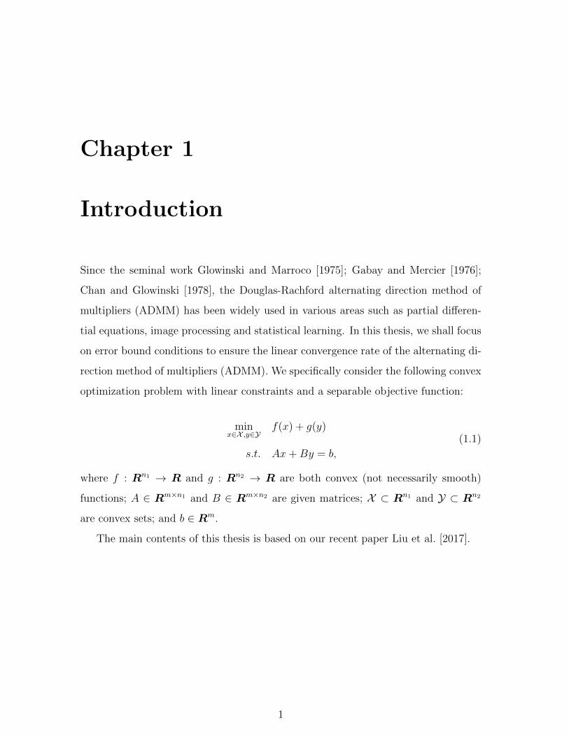
rection method of multipliers (ADMM). We specifically consider the following convex

optimization problem with linear constraints and a separable objective function:

minx∈X ,y∈Y

f(x) + g(y)

s.t. Ax+By = b,

(1.1)

where f : Rn1 → R and g : Rn2 → R are both convex (not necessarily smooth)

functions; A ∈ Rm×n1 and B ∈ Rm×n2 are given matrices; X ⊂ Rn1 and Y ⊂ Rn2

are convex sets; and b ∈ Rm.

The main contents of this thesis is based on our recent paper Liu et al. [2017].

1

1.1 Alternating Direction Method of Multipliers

(ADMM)

The iterative scheme of ADMM for (1.1) is:

xk+1 = arg min

x∈Xf(x)− (λk)T (Ax+Byk − b) +

β

2‖Ax+Byk − b‖2,

yk+1 = arg miny∈Yg(y)− (λk)T (Axk+1 +By − b) +

β

2‖Axk+1 +By − b‖2,

λk+1 = λk − β(Axk+1 +Byk+1 − b),

(1.2)

where λ is the Lagrange multiplier and β > 0 is a penalty parameter. The subprob-

lems arising in ADMM’s iterations may be much easier than the original problem (1.1)

and indeed they may have closed-form solutions when f and g are special enough.

This feature makes the implementation of ADMM extremely easy for some appli-

cations arising in areas such as compressive sensing, image processing, statistical

learning, sparse and low-rank optimization problems, etc., and it well explains the

popularity of ADMM in various areas. We refer to Boyd et al. [2011]; Eckstein and

Yao [2015]; Glowinski [2014] for some review papers on the ADMM.

Under some mild conditions such as the nonemptyness of the solution set of the

problem (1.1), the convergence of ADMM has been well studied in earlier literature,

see e.g., Eckstein and Bertsekas [1992]; Eckstein et al. [1990]; Fortin and Glowinski

[2000]; Gabay and Mercier [1976]; Glowinski and Le Tallec [1989]; Glowinski and

Marroco [1975]; He and Yang [1998]; Lions and Mercier [1979]. Because of the appli-

cations recently found in various areas, research on the convergence analysis of the

ADMM has regained attention from the community and more efforts have been put

on the convergence rate analysis. In He and Yuan [2012, 2015]; Monteiro and Svaiter

[2013], the worst-case O(1/k) convergence rate measured by the iteration complex-

ity has been established for the ADMM in both the ergodic and nonergodic senses,

where k is the iteration counter. Such a convergence rate is of sublinear. Conse-

quently, some results for the linear convergence rate of ADMM have been established

either for special cases of the generic model (1.1) or for the scenarios where more

assumptions are posed on the model (1.1). For example, it is shown in [Boley, 2013,

2

Theorem 6.4] that the local linear convergence rate of ADMM can be guaranteed

for the special linear and quadratic cases of (1.1), if it is assumed that both the

minimization subproblems in (1.2) have unique optimal solutions and additionally

some strict complementarity conditions hold. Moreover, if f and/or g are/is strongly

convex, one of them is differentiable and has a Lipschitz continuous gradient, and the

generated iterative sequence is assumed to be bounded, together with some full rank

conditions of the coefficient matrices, the global linear convergence rate of ADMM is

proved in Deng and Yin [2016]. More results can be found in Nishihara et al. [2015]

as well.

As in He and Yuan [2012], instead of the original ADMM scheme (1.2), our analysis

is for the slightly generalized proximal version of the ADMM (PADMM for short)

xk+1 = arg min

x∈Xf(x)− (λk)T (Ax+Byk − b) +

β

2‖Ax+Byk − b‖2 +

1

2‖x− xk‖2D,

yk+1 = arg miny∈Y

g(y)− (λk)T (Axk+1 +By − b) +β

2‖Axk+1 +By − b‖2,

λk+1 = λk − β(Axk+1 +Byk+1 − b),(1.3)

where D ∈ Rn1×n1 is a symmetric and positive semi-definite matrix. Here, we slightly

abuse the notation ‖x‖2D for the number xTDx even though D may be only positive

semi-definite. Throughout the penalty parameter β is fixed in our discussion. This

scheme includes the original ADMM scheme (1.2) and the linearized ADMM (or,

split inexact Uzawa method in Zhang et al. [2010]) as special cases with D = 0 and

D = (σIn1−βATA) with σ > β‖ATA‖, respectively. Note that the linearized version

of ADMM has found many efficient applications, see Liu et al. [2013]; Wang and Yuan

[2012]; Yang and Yuan [2013] to mention a few. Hence, we include this case into our

discussion and consider the PADMM (1.3).

1.2 Error Bound Conditions for ADMM

Error bound conditions turn out to play an important role in studying the linear

convergence rate of ADMM. To elucidate on error bound conditions, we first mention

3

the Karush-Kuhn-Tucker (KKT) system of the problem (1.1):0 ∈ ∂f(x)− ATλ+NX (x),

0 ∈ ∂g(y)−BTλ+NY(y),

0 = Ax+By − b,

(1.4)

where “∂” denotes the subgradient of a convex function and NC(c) := ξ : 〈ξ, ζ−c〉 ≤

0, ∀ζ ∈ C denotes the normal cone at c to a given convex set C. Let S∗ be the

solution set of the KKT system (1.4) and assume it to be nonempty. Furthermore,

let r : Rn1 ×Rn2 ×Rm → R+ be a residual error function satisfying r(x, y, λ) = 0 iff

(x, y, λ) ∈ S∗. We say that the KKT system (1.4) admits a local error bound around

a given point (x∗, y∗, λ∗) ∈ S∗ with the residual error function r(x, y, λ) if there exist

a neighborhood

Bε(x∗, y∗, λ∗) := (x, y, λ) : ‖(x, y, λ)− (x∗, y∗, λ∗)‖ ≤ ε

of the point (x∗, y∗, λ∗) and a constant κ > 0 such that

[EBr] dist((x, y, λ), S∗) ≤ κ ·r(x, y, λ) provided (x, y, λ) ∈ Bε(x∗, y∗, λ∗). (1.5)

Throughout, we define dist(c, C) := infc′∈C‖c−c′‖ for a given subset C and vector c

in the same space, and ‖·‖ is the 2-norm without otherwise specified. If this estimate is

valid for every (x, y, λ) ∈ Rn1×Rn2×Rm, rather than merely (x, y, λ) ∈ Bε(x∗, y∗, λ∗),

we say that the KKT system (1.4) admits a global error bound.

Error bound conditions of the KKT system (1.4) with various choices of the

residual error function r(x, y, λ) have inspired some works for studying the linear

convergence rate of the ADMM. According to (1.4), it is natural to define an mapping

φ : Rn1 ×Rn2 ×Rm ⇒ Rn1 ×Rn2 ×Rm as

φ(x, y, λ) =

∂f(x)− ATλ+NX (x)

∂g(y)−BTλ+NY(y)

Ax+By − b

(1.6)

4

and then a residual error function as r(x, y, λ) = dist(0, φ(x, y, λ)). We call φ defined

in (1.6) the KKT mapping for obvious reasons and the KKT system (1.4) can be

written as 0 ∈ φ(x, y, λ). With φ(x, y, λ) given in (1.6), let us define S : Rn1 ×Rn2 ×

Rm ⇒ Rn1 ×Rn2 ×Rm as

S(p) := (x, y, λ) | p ∈ φ(x, y, λ) (1.7)

with p = (p1, p2, p3) ∈ Rn1 ×Rn2 ×Rm. Obviously, S(0) = S∗. Recall that we are

interested in finding 0 ∈ φ(x, y, λ), i.e., (x, y, λ) ∈ S(0) = (x, y, λ) | 0 ∈ φ(x, y, λ).

Hence, p in (1.7) plays the role of a perturbation parameter and (1.7) can be regarded

as a perturbed system of the KKT system (1.4). This is also the reason we purposively

use the same letter S to define the mapping in (1.7) in addition to the notation S∗

for the solution set of the KKT system (1.4).

Let us use the notation w = (x, y, λ) for a more compact presentation. Now, using

dist(0, φ(w)) as the residual error function, the KKT system (1.4) is said to admit a

local error bound around a feasible point w = (x, y, λ) if there exist a neighborhood

Bε(w) of w and some constant κ > 0 such that

[FEB] dist(w, S(0)) ≤ κ · dist(0, φ(w)) provided w ∈ Bε(w). (1.8)

Indeed, in terms of variational analysis, the existence of an error bound around the

reference point w with the residual error function r(w) = dist(0, φ(w)) is exactly the

metric subregularity of the KKT mapping φ(w) at (w, 0). The set-valued mapping

φ(w) is called metrically subregular around (w, 0) if there exists a neighbourhood

Bε(w) of w and κ > 0 such that

dist(w, φ−1 (0)

)≤ κ · dist (0, φ (w)) provided w ∈ Bε(w).

Equivalently, φ(w) is metrically subregular around (w, 0) if there exist a neighbour-

hood Bε(w) of w and κ > 0 such that

S (p) ∩ Bε(w) ⊂ S (0) + κ ‖p‖ · B1(0), ∀p, (1.9)

5

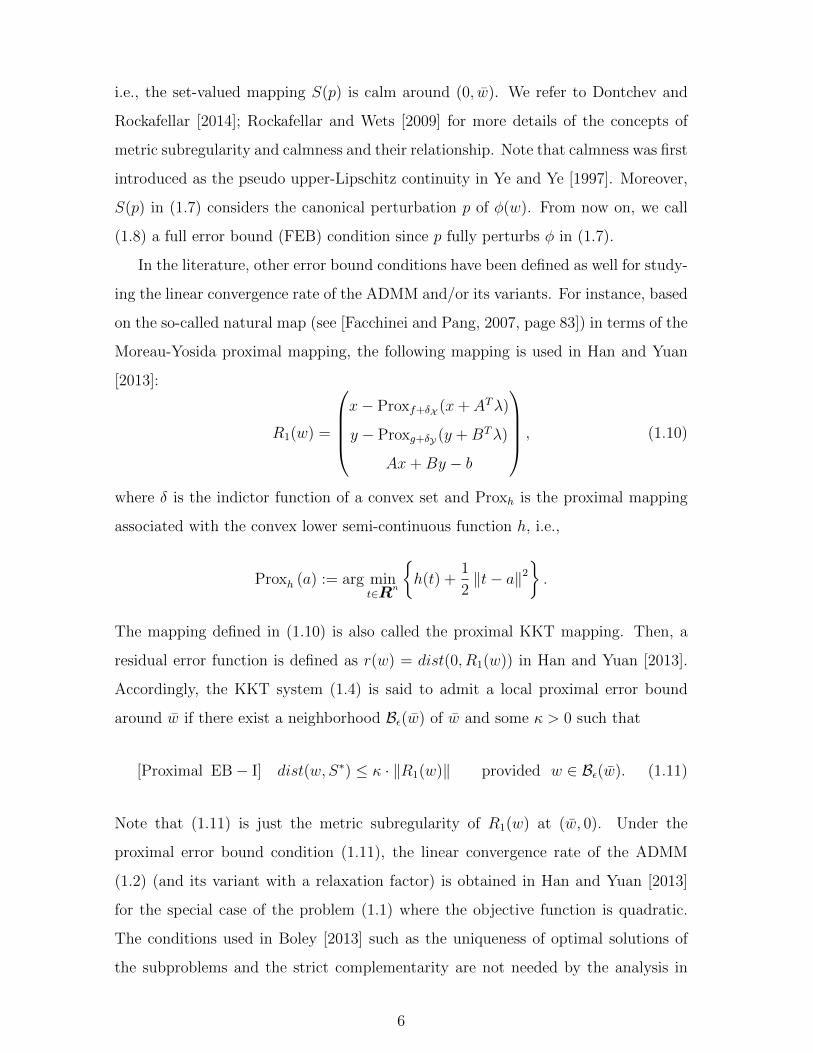
i.e., the set-valued mapping S(p) is calm around (0, w). We refer to Dontchev and

Rockafellar [2014]; Rockafellar and Wets [2009] for more details of the concepts of

metric subregularity and calmness and their relationship. Note that calmness was first

introduced as the pseudo upper-Lipschitz continuity in Ye and Ye [1997]. Moreover,

S(p) in (1.7) considers the canonical perturbation p of φ(w). From now on, we call

(1.8) a full error bound (FEB) condition since p fully perturbs φ in (1.7).

In the literature, other error bound conditions have been defined as well for study-

ing the linear convergence rate of the ADMM and/or its variants. For instance, based

on the so-called natural map (see [Facchinei and Pang, 2007, page 83]) in terms of the

Moreau-Yosida proximal mapping, the following mapping is used in Han and Yuan

[2013]:

R1(w) =

x− Proxf+δX (x+ ATλ)

y − Proxg+δY (y +BTλ)

Ax+By − b

, (1.10)

where δ is the indictor function of a convex set and Proxh is the proximal mapping

associated with the convex lower semi-continuous function h, i.e.,

Proxh (a) := arg mint∈Rn

h(t) +

1

2‖t− a‖2

.

The mapping defined in (1.10) is also called the proximal KKT mapping. Then, a

residual error function is defined as r(w) = dist(0, R1(w)) in Han and Yuan [2013].

Accordingly, the KKT system (1.4) is said to admit a local proximal error bound

around w if there exist a neighborhood Bε(w) of w and some κ > 0 such that

[Proximal EB− I] dist(w, S∗) ≤ κ · ‖R1(w)‖ provided w ∈ Bε(w). (1.11)

Note that (1.11) is just the metric subregularity of R1(w) at (w, 0). Under the

proximal error bound condition (1.11), the linear convergence rate of the ADMM

(1.2) (and its variant with a relaxation factor) is obtained in Han and Yuan [2013]

for the special case of the problem (1.1) where the objective function is quadratic.

The conditions used in Boley [2013] such as the uniqueness of optimal solutions of

the subproblems and the strict complementarity are not needed by the analysis in

6

Han and Yuan [2013].

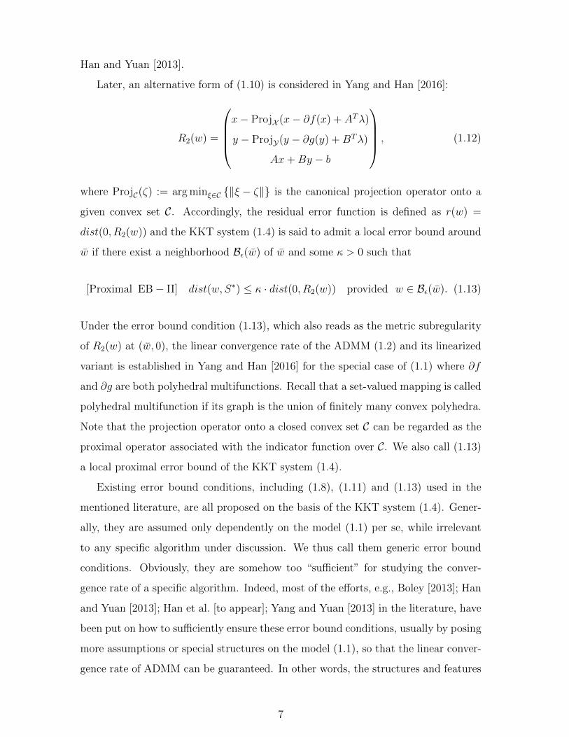
Later, an alternative form of (1.10) is considered in Yang and Han [2016]:

R2(w) =

x− ProjX (x− ∂f(x) + ATλ)

y − ProjY(y − ∂g(y) +BTλ)

Ax+By − b

, (1.12)

where ProjC(ζ) := arg minξ∈C ‖ξ − ζ‖ is the canonical projection operator onto a

given convex set C. Accordingly, the residual error function is defined as r(w) =

dist(0, R2(w)) and the KKT system (1.4) is said to admit a local error bound around

w if there exist a neighborhood Bε(w) of w and some κ > 0 such that

[Proximal EB− II] dist(w, S∗) ≤ κ · dist(0, R2(w)) provided w ∈ Bε(w). (1.13)

Under the error bound condition (1.13), which also reads as the metric subregularity

of R2(w) at (w, 0), the linear convergence rate of the ADMM (1.2) and its linearized

variant is established in Yang and Han [2016] for the special case of (1.1) where ∂f

and ∂g are both polyhedral multifunctions. Recall that a set-valued mapping is called

polyhedral multifunction if its graph is the union of finitely many convex polyhedra.

Note that the projection operator onto a closed convex set C can be regarded as the

proximal operator associated with the indicator function over C. We also call (1.13)

a local proximal error bound of the KKT system (1.4).

Existing error bound conditions, including (1.8), (1.11) and (1.13) used in the

mentioned literature, are all proposed on the basis of the KKT system (1.4). Gener-

ally, they are assumed only dependently on the model (1.1) per se, while irrelevant

to any specific algorithm under discussion. We thus call them generic error bound

conditions. Obviously, they are somehow too “sufficient” for studying the conver-

gence rate of a specific algorithm. Indeed, most of the efforts, e.g., Boley [2013]; Han

and Yuan [2013]; Han et al. [to appear]; Yang and Yuan [2013] in the literature, have

been put on how to sufficiently ensure these error bound conditions, usually by posing

more assumptions or special structures on the model (1.1), so that the linear conver-

gence rate of ADMM can be guaranteed. In other words, the structures and features

7

of an specific algorithm are ignored when its linear convergence rate is studied via

error bound conditions; and thus directly using these generic error bound conditions

indeed shrinks the range that validates the linear convergence rate of ADMM.

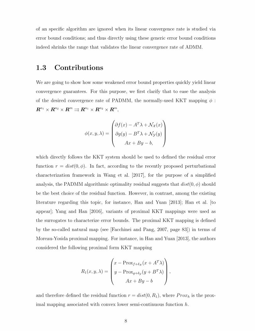
1.3 Contributions

We are going to show how some weakened error bound properties quickly yield linear

convergence guarantees. For this purpose, we first clarify that to ease the analysis

of the desired convergence rate of PADMM, the normally-used KKT mapping φ :

Rn1 ×Rn2 ×Rm ⇒ Rn1 ×Rn2 ×Rm,

φ(x, y, λ) =

∂f(x)− ATλ+NX (x)

∂g(y)−BTλ+NY(y)

Ax+By − b,

which directly follows the KKT system should be used to defined the residual error

function r = dist(0, φ). In fact, according to the recently proposed perturbational

characterization framework in Wang et al. [2017], for the purpose of a simplified

analysis, the PADMM algorithmic optimality residual suggests that dist(0, φ) should

be the best choice of the residual function. However, in contrast, among the existing

literature regarding this topic, for instance, Han and Yuan [2013]; Han et al. [to

appear]; Yang and Han [2016], variants of proximal KKT mappings were used as

the surrogates to characterize error bounds. The proximal KKT mapping is defined

by the so-called natural map (see [Facchinei and Pang, 2007, page 83]) in terms of

Moreau-Yosida proximal mapping. For instance, in Han and Yuan [2013], the authors

considered the following proximal form KKT mapping

R1(x, y, λ) =

x− Proxf+δX (x+ ATλ)

y − Proxg+δY (y +BTλ)

Ax+By − b

,

and therefore defined the residual function r = dist(0, R1), where Proxh is the prox-

imal mapping associated with convex lower semi-continuous function h.

8

The natural map has some advantages (see Facchinei and Pang [2007]) and the

usefulness of the proximal map-based error bound can be seen from the existing

literatures. However, according to the clarification in Wang et al. [2017], the residual

error function should be defined algorithm-tailored, and the proximal form mapping

does not match PADMM very appropriately.

In the language of variational analysis, the existence of an error bound with resid-

ual function r = dist(0, φ) is exactly “metric subregularity” of the KKT mapping φ.

The metric subregularity is equivalent to the calmness at the origin of the inverse of

the KKT mapping. In the recent paper Drusvyatskiy and Lewis [2016], the authors

investigate unconstrained separable convex optimization problem and illustrate that

subregularity of the gradient-like mapping is equivalent to subregularity of its sub-

differetial (see also Wang et al. [2017] from another perspective). Therefore, they

employ the quadratic growth condition as the characterization of error bound condi-

tion which succeeds to yield a linear rate convergence for the prox-gradient method.

In this thesis, for the constrained problem, we will show that the error bound defined

in terms of the KKT mapping φ is equivalent to the one of the proximal KKT mapping

R1. This observation thereby allows people to call on extensive literature relating the

metric regularity/subregularity of KKT mapping φ, see e.g., Gfrerer [2013]; Gfrerer

and Klatte [2016]; Gfrerer and Mordukhovich [2017]; Gfrerer and Ye [2017]; Henrion

et al. [2002].

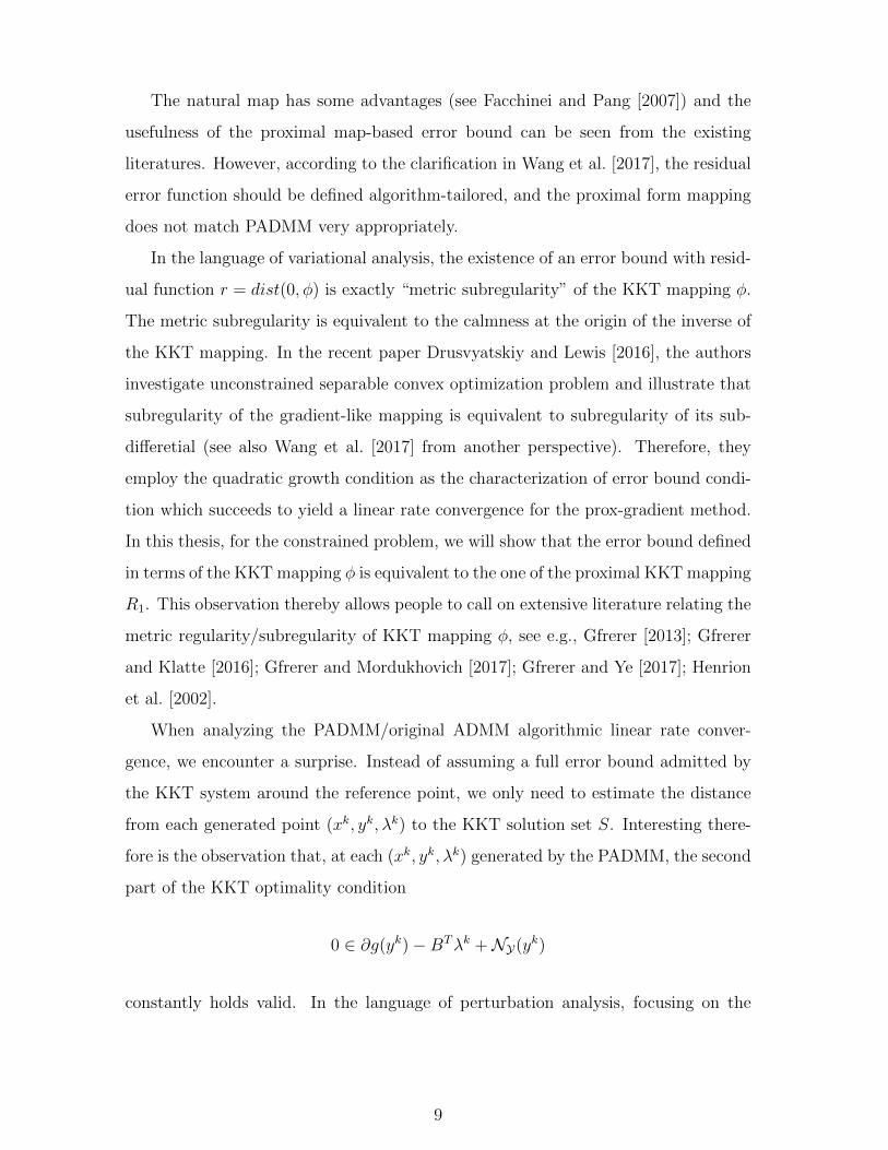
When analyzing the PADMM/original ADMM algorithmic linear rate conver-

gence, we encounter a surprise. Instead of assuming a full error bound admitted by

the KKT system around the reference point, we only need to estimate the distance

from each generated point (xk, yk, λk) to the KKT solution set S. Interesting there-

fore is the observation that, at each (xk, yk, λk) generated by the PADMM, the second

part of the KKT optimality condition

0 ∈ ∂g(yk)−BTλk +NY(yk)

constantly holds valid. In the language of perturbation analysis, focusing on the

9

sequence (xk, yk, λk), no perturbation occurs in the part

0 ∈ ∂g(y)−BTλ+NY(y)

of the KKT system 0 ∈ φ(x, y, λ). Inspired by this observation, we will show that the

weaker partial error bound is sufficient to ensure the desired linear rate convergence.

One example is presented to demonstrate the advantages of using the partial error

bound.

The new application of (partial) error bound thereby allows us to call on ex-

tensive literature concerning the metric subregularity of KKT mapping φ. Given

the generality of these techniques, we expect that the approach we describe here,

rooted in understanding linear convergence through natural (partial) KKT mapping,

should motivate broad investigation on calmness of multifunction to be employed.

In fact, the study on the calmness condition has enjoyed a prosperous time since

the recent paper Gfrerer [2011] of significance. We refer the reader to Gfrerer and

Mordukhovich [2015]; Gfrerer and Outrata [2016]; Gfrerer and Ye [2017] for several

very recent advance on this subject.

An important byproduct of our analysis, worthy of independent interest, relates to

the fact that our partial error bound theory may help interpret the convergence rate

change affected by updating order. Particularly, it is known that the updating order

of primal variables has nothing to do with the algorithmic convergence. However,

the updating order should interfere with the position where perturbation occurs and

hence the expression of partial error bound. That is, if we update y in front of x in

the PADMM, then at each (xk, yk, λk) generated by the PADMM, the first part of

the KKT optimality condition

0 ∈ ∂f(xk)− ATλk +NX (xk)

constantly holds valid. Therefore, it is possible for people to choose an appropriate

updating order such that the associated partial error bound is somehow easier to

meet. By doing so, one may attain a convergence rate guarantee in theory.

10

1.4 Outline of the Thesis

In Chapter 2, we summarize some necessary preliminaries concerning global conver-

gence of ADMM.

In Chapter 3, we propose an error bound condition tailored for the specific iter-

ative scheme (1.3) and prove that it suffices to ensure the linear convergence of the

PADMM (1.3). We also show that the generic FEB (1.8) is sufficient to ensure this

error bound condition.

In Chapter 4, we clarify the equivalence between the FEB (1.8) and the proximal

EB-I (1.11) and proximal EB-II (1.13). Because of the equivalence, theoretically we

can choose anyone from (1.8), (1.11) and (1.13). We further explain in this chapter

why we choose the FEB (1.8) to conduct the convergence analysis for the PADMM

(1.3) from a perturbation analysis perspective.

In Chapter 5, with the purpose of studying PADMM-tailored error bound con-

ditions, we find that a more meticulous analysis for the sequence generated by (1.3)

immediately gives us an insight and helps us further weaken the mentioned error

bound conditions but still ensure the linear convergence rate of the PADMM (1.3).

More specifically, for the sequence wk generated by (1.3), the second part of the

KKT system (1.4), i.e., 0 ∈ ∂g(yk)−BTλk +NY(yk), always holds for all iterates. In

language of perturbation analysis, the sequence wk generated by the PADMM (1.3)

introduces no perturbation to the part 0 ∈ ∂g(y)−BTλ+NY(y) in (1.7). This inter-

esting observation suggests that there is no need to fully satisfy a general error bound

condition that is derived based on the KKT system (1.4) and a partial error bound

condition without consideration of the perturbation to the part ∂g(y)−BTλ+NY(y)

is sufficient for studying the linear convergence rate of the PADMM (1.3). In partic-

ular, an example is constructed to illustrate that the partial error bound condition is

indeed weaker than the known full counterparts.

In Chapter 6, we interpret the observation that the updating order may affect

convergence rate by the PADMM-tailored partial error bound condition. It has been

empirically observed that the convergence speed may be different if we swap the

order of x and y in the ADMM (1.2) despite that there is no difference from the

theoretical convergence-proof point of view. So far it seems that no rigorous theory

11

is known for explaining this difference. We shall show by an example that swapping

the order of x and y in (1.2) does make difference in satisfying the partial error bound

condition tailored for the ADMM (1.2). This theoretical justification gives hints to

users to decide a more appropriate order of updating the primal variables for a specific

application of the problem (1.1) so that the associated partial error bound can be

meet more easily and hence the linear convergence rate of ADMM can be yielded.

In Chapter 7, we mention some conclusions and possible future works.

12

Chapter 2

Preliminaries

In this Chapter, we state assumptions under which our further analysis will be con-

ducted, recall the variational inequality characterization of the problem (1.1) and

provide some known or obvious convergence results of the PADMM (1.3).

2.1 Basic Assumptions

To characterize the solution set of the problem (1.1) by the first-order optimality

conditions, we need certain constraint qualification such as the strong conical hull

intersection property (Strong CHIP for short) for the sets X × Y and F defined by

F := (x, y) | Ax+By = b. (2.1)

In particular, for any (x, y) feasible for the problem (1.1), there holds

NF∩X×Y(x, y) := NF(x, y) +NX (x)×NY(y).

The strong CHIP plays a similar role as the Abadie constraint qualification, which

is regarded as not restrictive. Throughout, to avoid triviality, the following nonemp-

tyness assumption is assumed.

Assumption 2.1. The optimal solution set of problem (1.1) is nonempty.

Under Assumption 2.1 and strong CHIP, (x∗, y∗) ∈ X × Y is an optimal solution

13

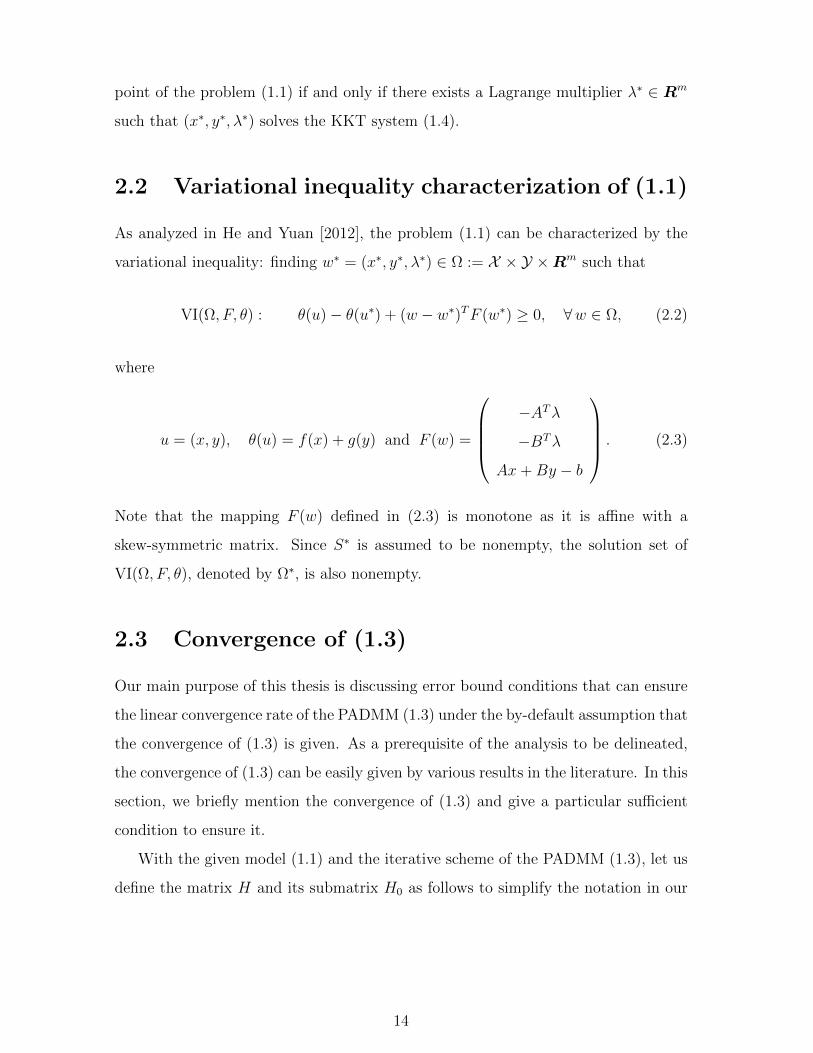
point of the problem (1.1) if and only if there exists a Lagrange multiplier λ∗ ∈ Rm

such that (x∗, y∗, λ∗) solves the KKT system (1.4).

2.2 Variational inequality characterization of (1.1)

As analyzed in He and Yuan [2012], the problem (1.1) can be characterized by the

variational inequality: finding w∗ = (x∗, y∗, λ∗) ∈ Ω := X × Y ×Rm such that

VI(Ω, F, θ) : θ(u)− θ(u∗) + (w − w∗)TF (w∗) ≥ 0, ∀w ∈ Ω, (2.2)

where

u = (x, y), θ(u) = f(x) + g(y) and F (w) =

−ATλ

−BTλ

Ax+By − b

. (2.3)

Note that the mapping F (w) defined in (2.3) is monotone as it is affine with a

skew-symmetric matrix. Since S∗ is assumed to be nonempty, the solution set of

VI(Ω, F, θ), denoted by Ω∗, is also nonempty.

2.3 Convergence of (1.3)

Our main purpose of this thesis is discussing error bound conditions that can ensure

the linear convergence rate of the PADMM (1.3) under the by-default assumption that

the convergence of (1.3) is given. As a prerequisite of the analysis to be delineated,

the convergence of (1.3) can be easily given by various results in the literature. In this

section, we briefly mention the convergence of (1.3) and give a particular sufficient

condition to ensure it.

With the given model (1.1) and the iterative scheme of the PADMM (1.3), let us

define the matrix H and its submatrix H0 as follows to simplify the notation in our

14

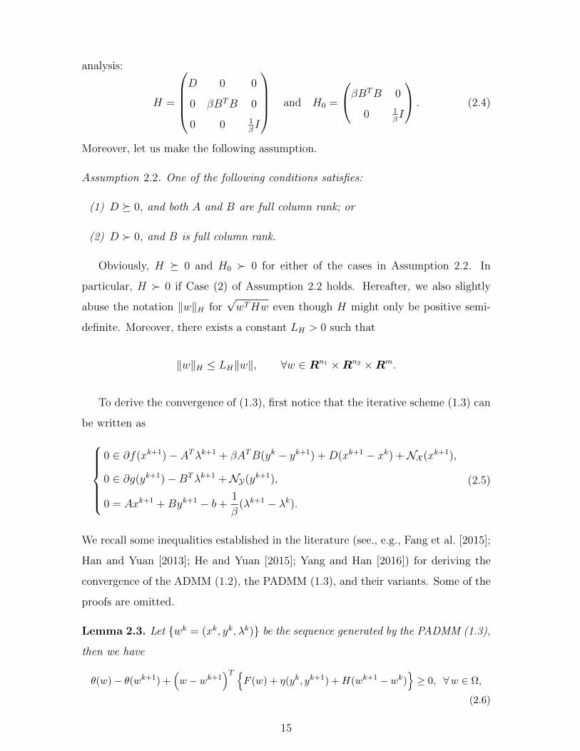
analysis:

H =

D 0 0

0 βBTB 0

0 0 1βI

and H0 =

βBTB 0

0 1βI

. (2.4)

Moreover, let us make the following assumption.

Assumption 2.2. One of the following conditions satisfies:

(1) D 0, and both A and B are full column rank; or

(2) D 0, and B is full column rank.

Obviously, H 0 and H0 0 for either of the cases in Assumption 2.2. In

particular, H 0 if Case (2) of Assumption 2.2 holds. Hereafter, we also slightly

abuse the notation ‖w‖H for√wTHw even though H might only be positive semi-

definite. Moreover, there exists a constant LH > 0 such that

‖w‖H ≤ LH‖w‖, ∀w ∈ Rn1 ×Rn2 ×Rm.

To derive the convergence of (1.3), first notice that the iterative scheme (1.3) can

be written as0 ∈ ∂f(xk+1)− ATλk+1 + βATB(yk − yk+1) +D(xk+1 − xk) +NX (xk+1),

0 ∈ ∂g(yk+1)−BTλk+1 +NY(yk+1),

0 = Axk+1 +Byk+1 − b+1

β(λk+1 − λk).

(2.5)

We recall some inequalities established in the literature (see., e.g., Fang et al. [2015];

Han and Yuan [2013]; He and Yuan [2015]; Yang and Han [2016]) for deriving the

convergence of the ADMM (1.2), the PADMM (1.3), and their variants. Some of the

proofs are omitted.

Lemma 2.3. Let wk = (xk, yk, λk) be the sequence generated by the PADMM (1.3),

then we have

θ(w)− θ(wk+1) +(w − wk+1

)T F (w) + η(yk, yk+1) +H(wk+1 − wk)

≥ 0, ∀w ∈ Ω,

(2.6)

15

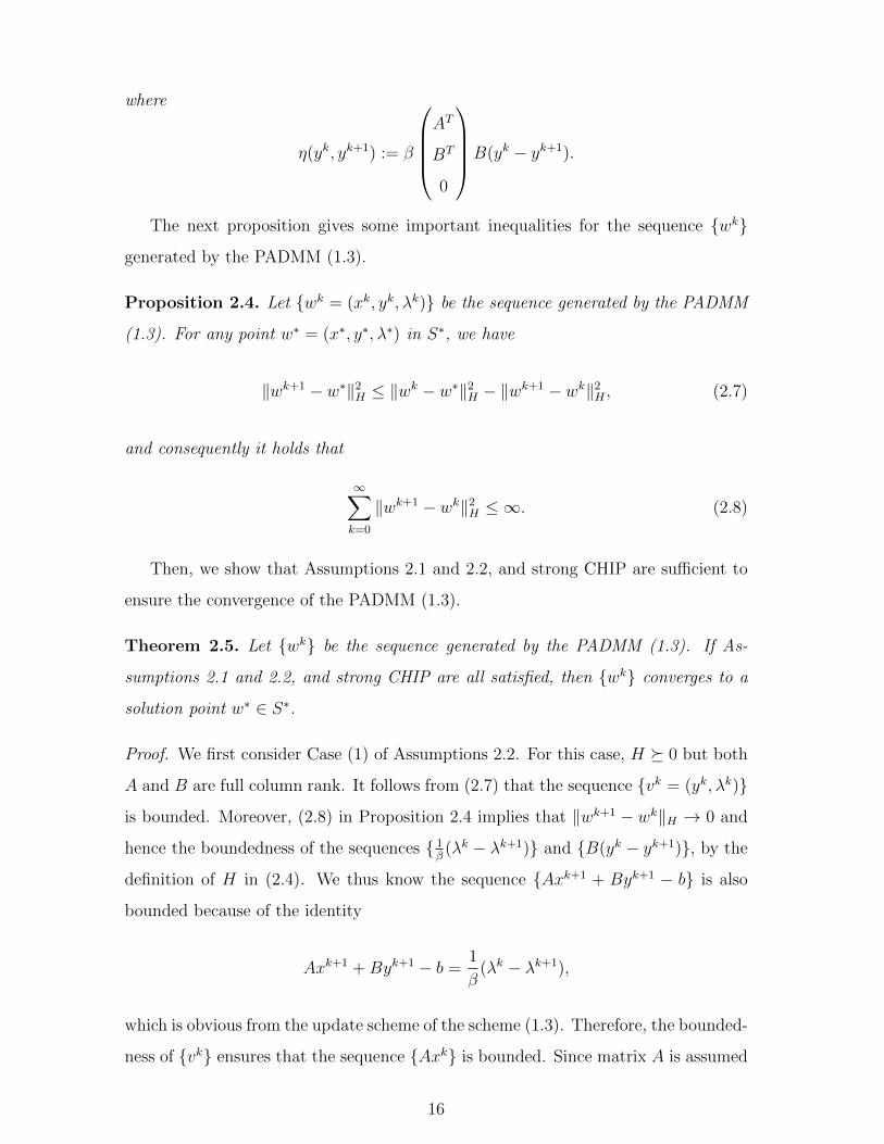
where

η(yk, yk+1) := β

AT

BT

0

B(yk − yk+1).

The next proposition gives some important inequalities for the sequence wk

generated by the PADMM (1.3).

Proposition 2.4. Let wk = (xk, yk, λk) be the sequence generated by the PADMM

(1.3). For any point w∗ = (x∗, y∗, λ∗) in S∗, we have

‖wk+1 − w∗‖2H ≤ ‖wk − w∗‖2

H − ‖wk+1 − wk‖2H , (2.7)

and consequently it holds that

∞∑k=0

‖wk+1 − wk‖2H ≤ ∞. (2.8)

Then, we show that Assumptions 2.1 and 2.2, and strong CHIP are sufficient to

ensure the convergence of the PADMM (1.3).

Theorem 2.5. Let wk be the sequence generated by the PADMM (1.3). If As-

sumptions 2.1 and 2.2, and strong CHIP are all satisfied, then wk converges to a

solution point w∗ ∈ S∗.

Proof. We first consider Case (1) of Assumptions 2.2. For this case, H 0 but both

A and B are full column rank. It follows from (2.7) that the sequence vk = (yk, λk)

is bounded. Moreover, (2.8) in Proposition 2.4 implies that ‖wk+1 − wk‖H → 0 and

hence the boundedness of the sequences 1β(λk − λk+1) and B(yk − yk+1), by the

definition of H in (2.4). We thus know the sequence Axk+1 + Byk+1 − b is also

bounded because of the identity

Axk+1 +Byk+1 − b =1

β(λk − λk+1),

which is obvious from the update scheme of the scheme (1.3). Therefore, the bounded-

ness of vk ensures that the sequence Axk is bounded. Since matrix A is assumed

16

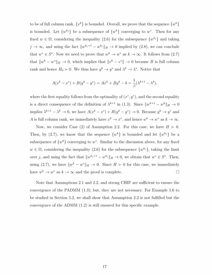
to be of full column rank, xk is bounded. Overall, we prove that the sequence wk

is bounded. Let wkj be a subsequence of wk converging to w∗. Then for any

fixed w ∈ Ω, considering the inequality (2.6) for the subsequence wkj and taking

j → ∞, and using the fact ‖wkj+1 − wkj‖H → 0 implied by (2.8), we can conclude

that w∗ ∈ S∗. Now we need to prove that wk → w∗ as k →∞. It follows from (2.7)

that ‖wk − w∗‖H → 0, which implies that ‖vk − v∗‖ → 0 because B is full column

rank and hence H0 0. We thus have yk → y∗ and λk → λ∗. Notice that

A(xk − x∗) +B(yk − y∗) = Axk +Byk − b =1

β(λk+1 − λk),

where the first equality follows from the optimality of (x∗, y∗), and the second equality

is a direct consequence of the definition of λk+1 in (1.3). Since ‖wk+1 − wk‖H → 0

implies λk+1 − λk → 0, we have A(xk − x∗) +B(yk − y∗)→ 0. Because yk → y∗ and

A is full column rank, we immediately have xk → x∗, and hence wk → w∗ as k →∞.

Now, we consider Case (2) of Assumption 2.2. For this case, we have H 0.

Then, by (2.7), we know that the sequence wk is bounded and let wkj be a

subsequence of wk converging to w∗. Similar to the discussion above, for any fixed

w ∈ Ω, considering the inequality (2.6) for the subsequence wkj, taking the limit

over j, and using the fact that ‖wkj+1 − wkj‖H → 0, we obtain that w∗ ∈ S∗. Then,

using (2.7), we have ‖wk − w∗‖H → 0. Since H 0 for this case, we immediately

have wk → w∗ as k →∞ and the proof is complete.

Note that Assumptions 2.1 and 2.2, and strong CHIP are sufficient to ensure the

convergence of the PADMM (1.3); but, they are not necessary. For Example 5.6 to

be studied in Section 5.2, we shall show that Assumption 2.2 is not fulfilled but the

convergence of the ADMM (1.2) is still ensured for this specific example.

17

Chapter 3

Algorithm-tailored error bound

conditions

In this section, with the by-default given convergence of the sequence wk generated

by the PADMM (1.3) to w∗ ∈ S∗, we focus on the discussion of its linear convergence

rate. Note that it is not necessary to assume Assumption 2.2 in the analysis.

As mentioned, in the literature, some generic error bound conditions depending

only on the model have been studied for the linear convergence rate of the ADMM

(1.2) and its variants; and in the literature, it is focused on how to sufficiently en-

sure these error bound conditions by posing more assumptions or requiring special

structures in the model (1.1). These error bound conditions or related study are

usually too restrictive; and they do not take into consideration the specific structures

and properties of the algorithm under discussion. Meanwhile, it seems beneficial to

estimate the error only for the specific iterative sequence, instead of arbitrary points

within a region, when the convergence rate of a particular algorithm is studied. We

hence prompt studying the linear convergence rate of the PADMM (1.3) under some

PADMM-tailored error bound conditions, with specific consideration of the iterative

scheme of (1.3). We shall show that this PADMM-tailored consideration can indeed

weaken the mentioned generic error bound conditions.

We first make some notation clear. Recall the definition of H in (2.4). We shall

use the notation

distH(w, C) := infw′∈C‖w − w′‖H, (3.1)

18

for a given subset C and vector w in the same space. As mentioned, H 0 under

Assumption 2.2. When distH(·, S∗) and dist(·, S∗) are considered, since

‖w‖2H = wTHw ≤ ρ(H)‖w‖2

2, ∀w ∈ Rn1 ×Rn2 ×Rm,

where ρ(H) is the spectral radius of matrix H. Let LH =√ρ(H), it follows from

(3.1) that

distH(w, S∗) ≤ LH · dist(w, S∗), ∀w ∈ Rn1 ×Rn2 ×Rm. (3.2)

Moreover, notice that the variable x is intermediate and it is not involved in the

iteration of the original ADMM (1.2); see, e.g., Boyd et al. [2011]. When our analysis

generally conducted for the PADMM (1.3) is specified for the original ADMM (1.2),

i.e. D = 0, we also need the notation v = (y, λ) to exclude the intermediate variable

x and S∗v := (y∗, λ∗) | (x∗, y∗, λ∗) ∈ S∗ for some x∗. Accordingly, H0 is needed to

present the analysis for (1.2) compactly; and instead of distH(w, S∗), we just use

distH0(v, S∗v) := inf

v′∈S∗v‖v − v′‖H0, (3.3)

when the original ADMM (1.2) is considered in our analysis. Also, we use the notation

S∗λ := λ∗ | (x∗, y∗, λ∗) ∈ S∗ for some (x∗, y∗) (3.4)

when the convergence of the sequence of Lagrange multiplier λk is highlighted.

3.1 PADMM-tailored error bound for the linear

convergence rate

We first present a PADMM-tailored error bound condition associated with the se-

quence generated by PADMM (1.3); and show that it suffices to guarantee the linear

convergence rate of the generated sequence. We refer to more literatures, e.g., Tao

and Yuan [to appear]; Wang et al. [2017], for some preliminary study of algorithm-

19

tailored error bound conditions for other algorithms.

Definition 3.1 (PADMM-tailored error bound). Let wk be the sequence generated

by the PADMM (1.3). If there exist κ > 0 and ε > 0 such that

distH(wk+1, S∗) ≤ κ · ‖wk+1 − wk‖H provided wk+1 ∈ Bε(w∗), (3.5)

then wk is said to satisfy a PADMM-tailored error bound.

With (3.5), it is easy to prove the local linear convergence rate for the PADMM

(1.3). We need one more theorem for preparation.

Theorem 3.2. Let wk be the sequence generated by the PADMM (1.3) and it

converge to w∗. If Assumptions 2.1 and strong CHIP are both satisfied, for any

ε > 0, there exists ε > 0 such that

‖wk+1 − wk‖H < ε =⇒ wk+1 ∈ Bε(w∗).

Proof. It follows from the convergence of wk that, for any ε > 0, there exists an

integer K > 0 such that

wk+1 ∈ Bε(w∗) ∀ k ≥ K.

Taking ε := min0≤k<K‖wk+1 − wk‖H > 0, we have

‖wk+1 − wk‖H < ε =⇒ k ≥ K =⇒ wk+1 ∈ Bε(w∗),

and the proof is complete.

We first prove a local property for the sequence dist2H(wk+1, S∗).

Theorem 3.3. Assume that Assumptions 2.1 and strong CHIP are both satisfied. If

the sequence wk generated by the PADMM (1.3) converges to w∗ and it satisfies

the PADMM-tailored error bound (3.5), then there exist κ > 0 and ε > 0 such that

dist2H(wk+1, S∗) ≤ (1 +1

κ2)−1 · dist2H(wk, S∗) provided ‖wk+1 − wk‖H < ε.

20

Proof. First, it follows from (2.7) that

dist2H(wk+1, S∗) ≤ dist2H(wk, S∗)− ‖wk+1 − wk‖2H , ∀k = 1, 2, . . . .

By virtue of Theorem 3.2 and (3.5), there exist κ > 0 and ε > 0 such that

distH(wk+1, S∗) ≤ κ · ‖wk+1 − wk‖2H provided ‖wk+1 − wk‖H < ε.

Subsequently, we have

dist2H(wk+1, S∗) ≤ dist2H(wk, S∗)− 1

κ2dist2H(wk+1, S∗) provided ‖wk+1 −wk‖H < ε,

and the proof is complete.

Moreover, we observe that when the convergence of sequence wk is guaranteed,

the local property of the sequence dist2H(wk+1, S∗) established in Theorem 3.3 is

essentially global. Hence, there is no difference in studying the local or global property

for the sequence dist2H(wk+1, S∗) under the PADMM-tailored error bound condition

(3.5). The following theorem is inspired by [Facchinei and Pang, 2007, Proposition

6.1.2].

Theorem 3.4. Assume that Assumptions 2.1 and strong CHIP are both satisfied. If

the sequence wk generated by the PADMM (1.3) converges to w∗ and it satisfies

the PADMM-tailored error bound condition (3.5), then there exists κ > 0 such that

dist2H(wk+1, S∗) ≤ (1 +1

κ2)−1 · dist2H(wk, S∗), ∀ k ≥ 0. (3.6)

Proof. Because of Theorem 3.3, there exist κ > 0 and ε > 0 such that

distH(wk+1, S∗) ≤ κ · ‖wk+1 − wk‖H provided ‖wk+1 − wk‖H < ε.

Thus, we only need to consider indices k such that ‖wk+1 − wk‖H ≥ ε. According

to (2.7), there is a constant M > 0 such that ‖wk − w∗‖H ≤ M for all k ≥ 0. We

21

immediately have

distH(wk+1, S∗) ≤ ‖wk+1−w∗‖H ≤M/ε·‖wk+1−wk‖H provided ‖wk+1−wk‖H ≥ ε.

Letting κ := maxκ,M/ε, we obtain that

distH(wk+1, S∗) ≤ κ · ‖wk+1 − wk‖H , ∀ k ≥ 0.

Together with (2.7), we have

dist2H(wk+1, S∗) ≤ (1 +1

κ2)−1 · dist2H(wk, S∗), ∀ k ≥ 0,

and the proof is complete.

Based on Theorem 3.4, the linear convergence rate of the sequence λk generated

by the PADMM (1.3) can be immediately derived. We summarize it in the following

theorem.

Theorem 3.5. Assume that Assumptions 2.1 and strong CHIP are both satisfied. If

the sequence wk generated by the PADMM (1.3) converges to w∗ and it satisfies

the PADMM-tailored error bound condition (3.5), then there exists κ > 0 such that

dist(λk, S∗λ) ≤ (1 +1

κ2)−

k2 · distH(w0, S∗), ∀ k ≥ 0,

where S∗λ is defined in (3.4). That is, the sequence λk generated by the PADMM

(1.3) converges linearly.

If the convergence of PADMM (1.3) is guaranteed specifically by Assumption

2.2 as discussed in Section 2.3, then accordingly we can further specify the linear

convergence rate of the PADMM (1.3) in the following two theorems. Note that the

linear convergence results established below are both global, because of Theorem 3.4.

Theorem 3.6 (Globally Linear Convergence Rate of vk). Let assumptions in The-

orem 3.4 hold; and additionally if Case (1) of Assumption 2.2 holds, then it follows

that

distH0(vk, S∗v) ≤ (1 +

1

κ2)−

k2 · distH(w0, S∗), ∀ k ≥ 0.

22

That is, the sequence vk generated by the PADMM (1.3) converges linearly.

Theorem 3.7 (Globally Linear Convergence Rate of wk). Let assumptions in

Theorem 3.4 hold; and additionally if Case (2) of Assumption 2.2 holds, then it

follows that

distH(wk, S∗) ≤ (1 +1

κ2)−

k2 · distH(w0, S∗), ∀ k ≥ 0.

That is, the sequence wk generated by the PADMM (1.3) converges linearly.

For the special case where D = 0, the PADMM (1.3) reduces to the original

ADMM (1.2). Theorem 3.6 indicates the linear convergence rate of the ADMM (1.2)

in sense of vk under Case (1) of Assumption 2.2, which is consistent with the

analysis in the ADMM literature. Recall that the variable x is intermediate and it

is not involved in the iteration performed by (1.2); hence convergence results of the

ADMM (1.2) are measured only by the variables y and λ, and x does not appear.

3.2 FEB (1.8) is sufficient to ensure (3.5)

In the last section, we have proved the linear convergence rate of PADMM (1.3) under

the PADMM-tailored error bound condition (3.5). Generally this condition cannot

be checked directly. But we shall show that the FEB (1.8) suffices to ensure (3.5);

hence (3.5) is theoretically weaker than (1.8).

Let us start with presenting a lemma which will be often used in the analysis

later. The proof is trivial by using the characterization of an iterate of the PADMM

(1.3) given in (2.5); it is thus omitted. We need one more matrix to simplify the

notation in the analysis:

H :=

D −βATB 0

0 0 0

0 0 1βI

. (3.7)

Lemma 3.8. Let wk be the sequence generated by the PADMM (1.3); φ(·) be

23

defined in (1.6) and H in (3.7). Then, we have

D(xk − xk+1)− βATB(yk − yk+1)

0

1β(λk − λk+1)

∈ φ(xk+1, yk+1, λk+1), (3.8)

or equivalently,

H(wk − wk+1) ∈ φ(xk+1, yk+1, λk+1). (3.9)

Based on (3.8), we immediately find that dist(0, φ(wk+1)) can be bounded by

‖wk+1 − wk‖H . This is shown in the following lemma.

Lemma 3.9. Let wk be the sequence generated by the PADMM (1.3); and φ(·) be

defined in (1.6). There exists L1 > 0 such that

dist(0, φ(wk+1)) ≤ L1‖wk+1 − wk‖H . (3.10)

Proof. It follows from (3.8) that

dist(0, φ(wk+1)) =(‖D(xk − xk+1)− βATB(yk − yk+1)‖2 + ‖ 1

β(λk − λk+1)‖2

) 12

≤ ‖D(xk − xk+1)− βATB(yk − yk+1)‖+ ‖ 1

β(λk − λk+1)‖

≤ ‖D(xk+1 − xk)‖+ ρ(A)√β‖√βB(yk+1 − yk)‖+

1√β‖ 1√

β(λk+1 − λk)‖

≤ (√ρ(D) + ρ(A)

√β +

1√β

)‖wk+1 − wk‖H ,

where ρ(D) ≥ 0 and ρ(A) ≥ 0 are the spectral radius of the matrices D and A,

respectively. Therefore, the assertion (3.10) is proved with L1 :=√ρ(D)+ρ(A)

√β+

1√β> 0.

Now, it becomes clear that the FEB (1.8) gives the relationship between the terms

dist(wk+1, S∗) and dist(0, φ(wk+1)), and thus effectively bridges the inequalities in

(3.2) and (3.10), and eventually ensures the PADMM-tailored error bound condition

(3.5). We give the full description in the following lemma. Our motivation of studying

the FEB (1.8) for the linear convergence rate of the PADMM (1.3) is indeed justified;

more details will be given in Chapter 4.

24

Lemma 3.10. Let wk be the sequence generated by the PADMM (1.3) and it con-

verges to w∗. Then the FEB (1.8) around w∗ ensures the PADMM-tailored error

bound condition (3.5).

Proof. It follows from (3.10) in Lemma 3.9 and the FEB (1.8) that there exist κ > 0

and ε > 0 such that

dist(wk+1, S(0)) ≤ κdist(0, φ(wk+1)) ≤ L1κ‖wk+1−wk‖H , provided wk+1 ∈ Bε(w∗).

According to (3.2), we know that distH(·, S∗) ≤ LH · dist(·, S∗) holds for LH > 0.

Thus, we have

distH(wk+1, S∗) ≤ LH · dist(wk+1, S(0)) ≤ LHL1κ‖wk+1 − wk‖H , wk+1 ∈ Bε(w∗),

and the proof is complete.

Remark 3.11. Recall the definitions of φ(·) in (1.6) and S(p) in (1.7); also note that

the sequence wk generated by the PADMM (1.3) ensures (3.8). Hence, the term

H(wk − wk+1) in (3.9) can be regarded as a perturbation p of S(p). Moreover, it

follows from (1.9) that the set-valued map S(p) is calm around (0, w) if and only if

there exist κ > 0, σ > 0 and a neighborhood Bε(w) of w such that

dist(w, S(0)) ≤ k‖p‖ provided w ∈ Bε(w) ∩ S(p), ‖p‖ < σ.

Then, because of (3.10), it is clear that the calmness of S(p), which is independent

of the iterative sequence wk generated by the PADMM (1.3), suffices to ensure the

algorithm-tailored error bound (3.5). Also, notice that the calmness of S(p) at (0, w)

is equivalent to the FEB (1.8) around w. Hence, it is rationale to study the FEB

(1.8) to ensure (3.5) for the PADMM (1.3). We refer to Wang et al. [2017] for a

more general study, in which an unified framework is proposed to develop appropriate

sufficient conditions for ensuring various error bound conditions that are tailored for

some algorithms.

Using Theorem 3.4 and Lemma 3.10, we immediately have the following theorem

and its proof is omitted.

25

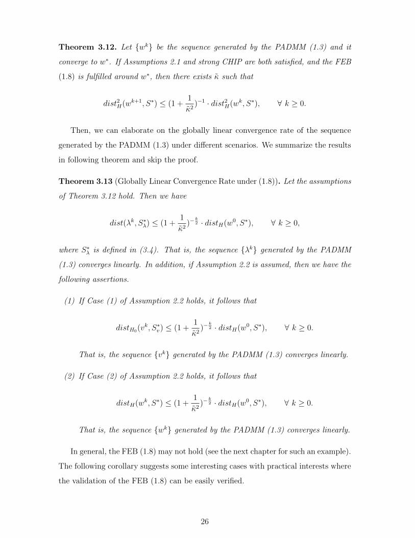
Theorem 3.12. Let wk be the sequence generated by the PADMM (1.3) and it

converge to w∗. If Assumptions 2.1 and strong CHIP are both satisfied, and the FEB

(1.8) is fulfilled around w∗, then there exists κ such that

dist2H(wk+1, S∗) ≤ (1 +1

κ2)−1 · dist2H(wk, S∗), ∀ k ≥ 0.

Then, we can elaborate on the globally linear convergence rate of the sequence

generated by the PADMM (1.3) under different scenarios. We summarize the results

in following theorem and skip the proof.

Theorem 3.13 (Globally Linear Convergence Rate under (1.8)). Let the assumptions

of Theorem 3.12 hold. Then we have

dist(λk, S∗λ) ≤ (1 +1

κ2)−

k2 · distH(w0, S∗), ∀ k ≥ 0,

where S∗λ is defined in (3.4). That is, the sequence λk generated by the PADMM

(1.3) converges linearly. In addition, if Assumption 2.2 is assumed, then we have the

following assertions.

(1) If Case (1) of Assumption 2.2 holds, it follows that

distH0(vk, S∗v) ≤ (1 +

1

κ2)−

k2 · distH(w0, S∗), ∀ k ≥ 0.

That is, the sequence vk generated by the PADMM (1.3) converges linearly.

(2) If Case (2) of Assumption 2.2 holds, it follows that

distH(wk, S∗) ≤ (1 +1

κ2)−

k2 · distH(w0, S∗), ∀ k ≥ 0.

That is, the sequence wk generated by the PADMM (1.3) converges linearly.

In general, the FEB (1.8) may not hold (see the next chapter for such an example).

The following corollary suggests some interesting cases with practical interests where

the validation of the FEB (1.8) can be easily verified.

26

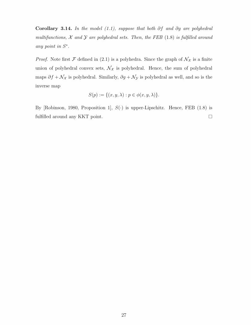
Corollary 3.14. In the model (1.1), suppose that both ∂f and ∂g are polyhedral

multifunctions, X and Y are polyhedral sets. Then, the FEB (1.8) is fulfilled around

any point in S∗.

Proof. Note first F defined in (2.1) is a polyhedra. Since the graph of NX is a finite

union of polyhedral convex sets, NX is polyhedral. Hence, the sum of polyhedral

maps ∂f +NX is polyhedral. Similarly, ∂g +NY is polyhedral as well, and so is the

inverse map

S(p) := (x, y, λ) : p ∈ φ(x, y, λ).

By [Robinson, 1980, Proposition 1], S(·) is upper-Lipschitz. Hence, FEB (1.8) is

fulfilled around any KKT point.

27

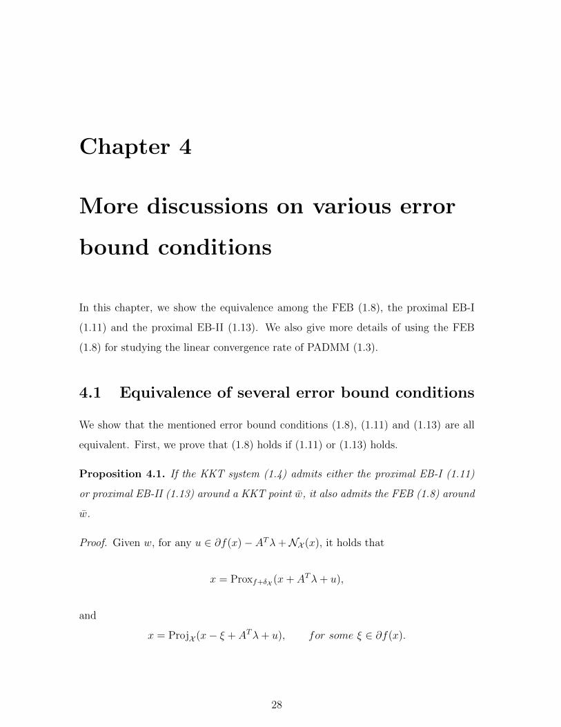
Chapter 4

More discussions on various error

bound conditions

In this chapter, we show the equivalence among the FEB (1.8), the proximal EB-I

(1.11) and the proximal EB-II (1.13). We also give more details of using the FEB

(1.8) for studying the linear convergence rate of PADMM (1.3).

4.1 Equivalence of several error bound conditions

We show that the mentioned error bound conditions (1.8), (1.11) and (1.13) are all

equivalent. First, we prove that (1.8) holds if (1.11) or (1.13) holds.

Proposition 4.1. If the KKT system (1.4) admits either the proximal EB-I (1.11)

or proximal EB-II (1.13) around a KKT point w, it also admits the FEB (1.8) around

w.

Proof. Given w, for any u ∈ ∂f(x)− ATλ+NX (x), it holds that

x = Proxf+δX (x+ ATλ+ u),

and

x = ProjX (x− ξ + ATλ+ u), for some ξ ∈ ∂f(x).

28

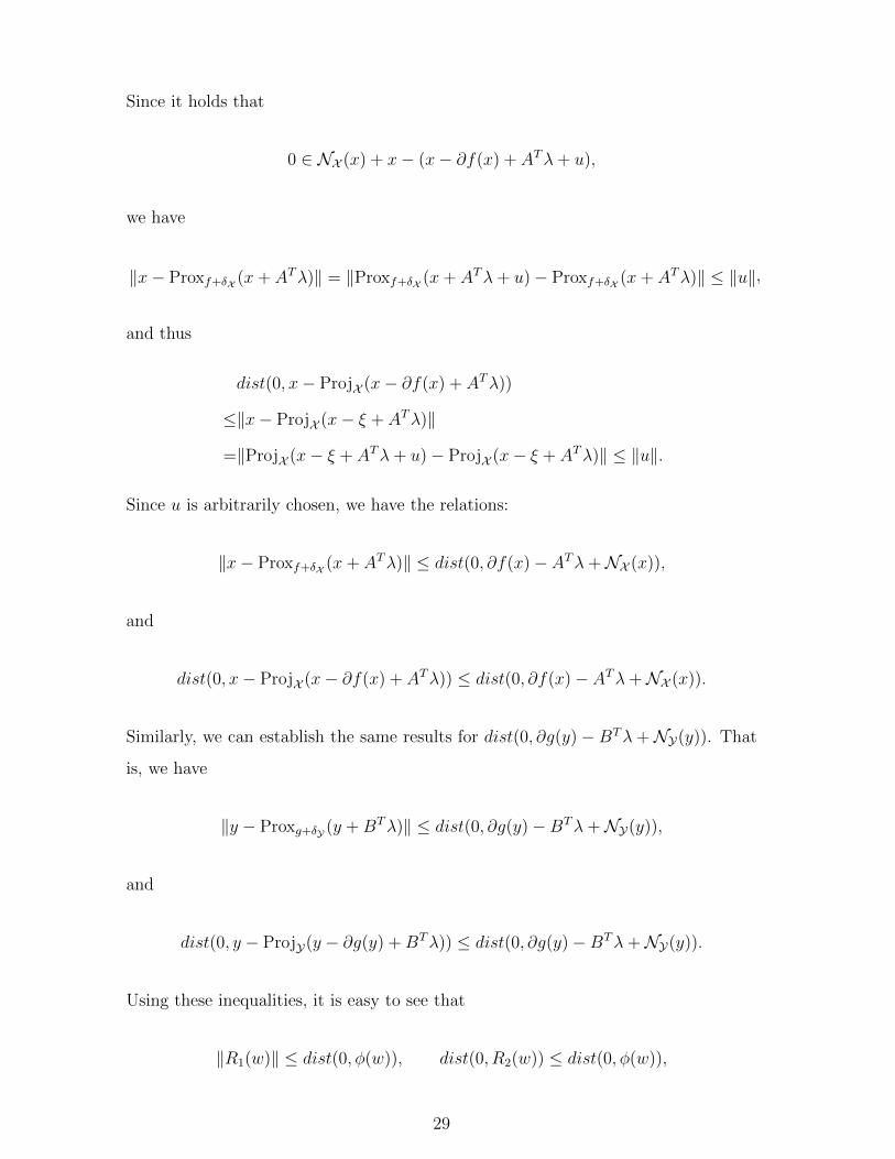
Since it holds that

0 ∈ NX (x) + x− (x− ∂f(x) + ATλ+ u),

we have

‖x− Proxf+δX (x+ ATλ)‖ = ‖Proxf+δX (x+ ATλ+ u)− Proxf+δX (x+ ATλ)‖ ≤ ‖u‖,

and thus

dist(0, x− ProjX (x− ∂f(x) + ATλ))

≤‖x− ProjX (x− ξ + ATλ)‖

=‖ProjX (x− ξ + ATλ+ u)− ProjX (x− ξ + ATλ)‖ ≤ ‖u‖.

Since u is arbitrarily chosen, we have the relations:

‖x− Proxf+δX (x+ ATλ)‖ ≤ dist(0, ∂f(x)− ATλ+NX (x)),

and

dist(0, x− ProjX (x− ∂f(x) + ATλ)) ≤ dist(0, ∂f(x)− ATλ+NX (x)).

Similarly, we can establish the same results for dist(0, ∂g(y)− BTλ +NY(y)). That

is, we have

‖y − Proxg+δY (y +BTλ)‖ ≤ dist(0, ∂g(y)−BTλ+NY(y)),

and

dist(0, y − ProjY(y − ∂g(y) +BTλ)) ≤ dist(0, ∂g(y)−BTλ+NY(y)).

Using these inequalities, it is easy to see that

‖R1(w)‖ ≤ dist(0, φ(w)), dist(0, R2(w)) ≤ dist(0, φ(w)),

29

and the proof is complete.

Notice the equality Proxth = (I + t∂h)−1. It is easy to show that (1.8) can imply

either (1.11) or (1.13) as well. We summarize this result in the following proposition.

Proposition 4.2. If the KKT system (1.4) admits the FEB (1.8) around a KKT

point w, it admits the proximal EB-I (1.11) and proximal EB-II (1.13) around w as

well.

Proof. First, by virtue of

x+ ATλ− Proxf+δX (x+ ATλ) ∈(∂f +NX

) (Proxf+δX (x+ ATλ)

),

y +BTλ− Proxg+δY (y +BTλ) ∈(∂g +NY

) (Proxg+δY (y +BTλ)

),

we conclude that

dist(

0, φ(Proxf+δX (x+ ATλ),Proxg+δY (y +BTλ), λ

))≤ ‖R1(w)‖. (4.1)

Therefore, for any w ∈ Bε(w), we have

dist(w, S(0)) ≤ c1(‖x− Proxf+δX (x+ ATλ)‖+ ‖y − Proxg+δY (y +BTλ)‖)

+ dist((

Proxf+δX (x+ ATλ),Proxg+δY (y +BTλ), λ), S(0)

)≤ c1(‖x− Proxf+δX (x+ ATλ)‖+ ‖y − Proxg+δY (y +BTλ)‖)

+ κ · dist(

0, φ(Proxf+δX (x+ ATλ),Proxg+δY (y +BTλ), λ

)),

≤ (2c1 + κ) · ‖R1(w)‖,

where the second inequality follows from the FEB (1.8), and the third inequality is

a direct consequence of (4.1). Thus we get the proximal EB-I (1.11) around w. We

can obtain the proximal EB-II (1.13) similarly. The proof is complete.

With Propositions 4.1 and 4.2, the equivalence between the FEB (1.8) and the

proximal EB-I (1.11) or proximal EB-II (1.13) is established. Technically one can

employ anyone of (1.8), (1.11) and (1.13), however, we just focus on the error bound

condition in form of (1.8). Together with the convergence rate analysis in the forth-

30

coming chapter, we will explain that (1.8) seems to be a better choice in the sense of

a simplified analysis later.

4.2 Preference of (1.8)

In this section we provide more details of why we prefer the FEB (1.8) than the

proximal EB-I (1.11) and proximal EB-II (1.13) for analyzing the linear convergence

rate of PADMM (1.3), despite of their theoretical equivalence.

As briefly mentioned preceding Lemma 3.10, to meet the PADMM-tailored error

bound condition (3.5), we need to bound the term distH(wk+1, S∗) by ‖wk+1−wk‖H .

On the other hand, the inequalities in (3.2) and (3.10) give us

distH(wk+1, S∗) ≤ LH · dist(wk+1, S∗), dist(0, φ(wk+1)) ≤ L1‖wk+1 − wk‖H .

Hence, essentially we need to build up the link between the terms dist(wk+1, S∗) and

dist(0, φ(wk+1)). This is perfectly achieved by the FEB (1.8).

For the proximal EB-I (1.11), however, it facilitates bridging the terms dist(wk+1, S∗)

and ‖R1(wk+1)‖; or the terms dist(wk+1, S∗) and dist(0, R2(wk+1)) by the proximal

EB-II (1.13). In other words, neither (1.11) nor (1.13) can be directly used for bridg-

ing the terms distH(wk+1, S∗) and ‖wk+1−wk‖H and hence ensuring (3.5); additional

and more complicated manipulations are needed if (1.11) or (1.13) is used.

Let us further explain the difference among these error bound conditions in

studying the linear convergence rate of the particular PADMM (1.3) from the per-

turbation perspective. As mentioned, the FEB (1.8) around a reference point w

is equivalent to the calmness of S(p) at (0, w). On the other hand, if we define

Sprox−I : Rn1 ×Rn2 ×Rm ⇒ Rn1 ×Rn2 ×Rm as

Sprox−I(p) :=

(x, y, λ) |

p1 ∈ (∂f +NX )(x− p1)− ATλ

p2 ∈ (∂g +NY)(y − p2)−BTλ

p3 = Ax+By − b

with p = (p1, p2, p3) ∈ Rn1 × Rn2 × Rm, then we have Sprox−I(0) = S∗ and hence

the proximal EB-I (1.11) around a reference point w is equivalent to the calmness of

31

Sprox−I(p) at (0, w). That is, there exist κ > 0, σ > 0 and a neighborhood Bε(w) of

w such that

dist(w, Sprox−I(0)) ≤ k‖p‖ provided w ∈ Bε(w) ∩ Sprox−I(p), ‖p‖ < σ.

Let us further define Sprox−II : Rn1 ×Rn2 ×Rm ⇒ Rn1 ×Rn2 ×Rm as

Sprox−II(p) :=

(x, y, λ) |

p1 ∈ ∂f(x)− ATλ+NX (x− p1)

p2 ∈ ∂g(y)−BTλ+NY(y − p2)

p3 = Ax+By − b

with p = (p1, p2, p3) ∈ Rn1 ×Rn2 ×Rm. It is easy to see that Sprox−II(0) = S∗ and

the proximal EB-II (1.13) around a reference point w is equivalent to the calmness

of Sprox−II(p) at (0, w). That is, there exist κ > 0, σ > 0 and a neighborhood Bε(w)

of w such that

dist(w, Sprox−II(0)) ≤ k‖p‖ provided w ∈ Bε(w) ∩ Sprox−II(p), ‖p‖ < σ.

According to Wang et al. [2017], for the sequence zk generated by an algorithm,

if H(zk+1 − zk) with an appropriate H is regarded as the perturbation of the cor-

responding optimality system, then the calmness of the induced set-valued mapping

straightforwardly implies the desirable error bound that is tailored for the algorithm

under investigation. When the PADMM (1.3) is considered, as shown by (3.8) in

Lemma 3.8, H(wk − wk+1) corresponds to the canonical perturbation of the KKT

system 0 ∈ φ(w). Hence, it is motivated to consider the perturbed multifunction

S(p) defined in (1.7), instead of Sprox−I(p) or Sprox−II(p). That is, we use the FEB

(1.8), rather than the proximal EB-I (1.11) or proximal EB-II (1.13), for analyzing

the linear convergence of the PADMM (1.3).

In addition to the superiority of yielding an easier analysis for the linear conver-

gence rate of the problem (1.1), studying the calmness of S(p), rather than Sprox−I(p)

or Sprox−II(p), may lead to some interesting future work, as we shall mention in Chap-

ter 7. Also, as we shall show soon in the next chapter, considering the perturbed

mapping S(p) in (1.7) enables us discern that the second part of the left-hand side

32

of (3.8) remains zero for each iteration of the PADMM (1.3). This insight inspires

us to study a partial error bound condition to ensure the linear convergence of the

PADMM (1.3), which seems to be novel in the literature.

33

Chapter 5

Partial error bound for the linear

convergence of PADMM (1.3)

We have established the linear convergence rate for the PADMM (1.3) under the

PADMM-tailored error bound condition (3.5) and shown that the FEB (1.8) suffi-

ciently ensures (3.5). In this chapter, we show that the FEB (1.8) can be further

weakened if the specific iterative scheme (1.3) is fully considered. As mentioned, this

is accomplished by the observation that there is no perturbation to the second part

of the perturbed mapping S(p) in (1.7). Hence, taking into consideration the specific

iterative scheme enables us to weaken the FEB (1.8) to guarantee (3.5) and hence

the linear convergence rate of the PADMM (1.3).

5.1 Partial error bound conditions and linear con-

vergence

Recall the KKT system (1.4) and the definition of the generic error bound condition

(1.5). Using the terminology initiated in Liu et al. [2008], we can also define the

so-called local partial error bound (PEB) for (1.4).

Definition 5.1. Assume S is represented as the intersection of two closed sets, i.e.,

S = C ∩ D. The KKT system (1.4) is said to admit a PEB on the set C around

w∗ ∈ S if there exists a nonnegative function r : Rn1 ×Rn2 ×Rm → R+ satisfying

34

r(w) = 0 if w ∈ D, a neighborhood Bε(w∗) of the point w∗, and a constant κ > 0 such

that

[PEBr on C] dist(w, S) ≤ κ · r(w) provided w ∈ Bε(w∗) ∩ C.

Obviously, from the definition, for any given closed set C, PEBr on C is weaker

than EBr defined in (1.5). Taking a closer look at (2.5) and (3.8), we notice that

the optimality condition with respect to y, i.e., 0 ∈ ∂g(y) − BTλ +NY(y), remains

satisfied for all iterates of (1.3). Let us define

Sg := w | 0 ∈ ∂g(y)−BTλ+NY(y).

Then, this observation motivates us to consider a partially perturbed KKT mapping

SP : Rn1 ×Rm ⇒ Rn1 ×Rn2 ×Rm as

SP (p) := w ∈ Sg | p ∈ φP (x, y, λ),

where φP : Rn1 ×Rn2 ×Rm ⇒ Rn1 ×Rm is defined as

φP (w) =

∂f(x)− ATλ+NX (x)

Ax+By − b

. (5.1)

Hence, we define a partial error bound that is particularly tailored for the specific

sequence wk generated by the PADMM (1.3). Note that this definition may not

be extended to other algorithms evidently.

Definition 5.2 (PADMM-tailored PEB). Let wk be the sequence generated by the

PADMM (1.3) and it converges to w∗. The KKT system (1.4) is said to admit a

partial local error bound around w∗ if there exists a neighborhood Bε(w∗) of w∗ and

some κ > 0 such that

[PEB] dist(w, SP (0)) ≤ κ · dist(0, φP (w)) provided w ∈ Sg ∩ Bε(w∗). (5.2)

Apparently, it holds that SP (0) = S(0) = S∗, and the following relationship is

easy to obtain: the proximal EB-I (1.11) and proximal EB-II (1.13) ⇔ the FEB

(1.8) ⇒ PADMM-tailored PEB (5.2). That is, the PADMM-tailored PEB (5.2) is

35

the weakest one.

We next show that the PADMM-tailored PEB (5.2) suffices to imply the (3.5)

and hence to ensure the linear convergence for the PADMM (1.3).

Lemma 5.3. Let wk be the sequence generated by the PADMM (1.3). If the

PADMM-tailored PEB (5.2) holds, then the PADMM-tailored error bound (3.5) holds

as well.

Proof. First, by virtue of (3.8) in Lemma 3.8, there always holds

0 ∈ ∂g(yk+1)−BTλk+1 +NY(yk+1),

which indicates that wk+1 ∈ Sg. Then by Lemma 3.9 (3.10), there is L1 > 0 such

that

dist(0, φP (wk+1)) ≤ L1‖wk+1 − wk‖H .

Furthermore, according to the PADMM-tailored PEB (5.2), it follows from wk+1 ∈ Sgthat there are κ > 0 and ε > 0 such that

dist(wk+1, S∗) = dist(wk+1, SP (0)) ≤ L1κ‖wk+1 − wk‖H , provided wk+1 ∈ Bε(w∗).

Then, it follows from (3.2) that distH(·, S∗) ≤ LH · dist(·, S∗) holds. Subsequently

the desired estimate follows

distH(wk+1, S∗) ≤ L2·dist(wk+1, S∗) ≤ L2L1κ‖wk+1−wk‖H , provided wk+1 ∈ Bε(w∗),

and the proof is complete.

Similar as the proof of Theorem 3.4, we can derive an important equality for the

sequence dist2H(wk+1, S∗) under (5.2).

Theorem 5.4. Let wk be the sequence generated by the PADMM (1.3) and it

converges to w∗. If Assumptions 2.1 and strong CHIP are both satisfied, and the

PADMM-tailored PEB (5.2) is fulfilled around w∗, then there exists κ such that

dist2H(wk+1, S∗) ≤ (1 +1

κ2)−1 · dist2H(wk, S∗), ∀ k ≥ 0.

36

Similar as Theorem 3.13, we can further specify Theorem 5.4 as the globally linear

convergence rate of the PADMM (1.3) under various scenarios. We present them in

the following theorem and skip the proof.

Theorem 5.5. Let wk be the sequence generated by the PADMM (1.3) and it

converges to w∗. If Assumptions 2.1 and strong CHIP are both satisfied, and the

PADMM-tailored PEB (5.2) is fulfilled around w∗, then there exists κ such that

dist(λk, S∗λ) ≤ (1 +1

κ2)−

k2 · distH(w0, S∗), ∀ k ≥ 0,

where S∗λ is defined in (3.4). That is, the sequence λk generated by the PADMM

(1.3) converges linearly. In addition, if Assumption 2.2 is assumed, then we have the

following assertions.

(1) If Case (1) of Assumption 2.2 holds, it follows that

distH0(vk, S∗v) ≤ (1 +

1

κ2)−

k2 · distH(w0, S∗), ∀ k ≥ 0. (5.3)

That is, the sequence vk generated by the PADMM (1.3) converges linearly.

• If Case (2) of Assumption 2.2 holds, it follows that

distH(wk, S∗) ≤ (1 +1

κ2)−

k2 · distH(w0, S∗), ∀ k ≥ 0. (5.4)

That is, the sequence wk generated by the PADMM (1.3) converges linearly.

5.2 Example

It is interesting to compare the FEB (1.8) and the PADMM-tailored PEB (5.2). We

next present an example which ensures the PADMM-tailored PEB (5.2) while fails to

guarantee the FEB (1.8) at its optimal solution point. Hence, together with the fact

that the FEB (1.8) being sufficient to guarantee the PADMM-tailored PEB (5.2), we

show that the PADMM-tailored PEB (5.2) is weaker than the FEB (1.8).

37

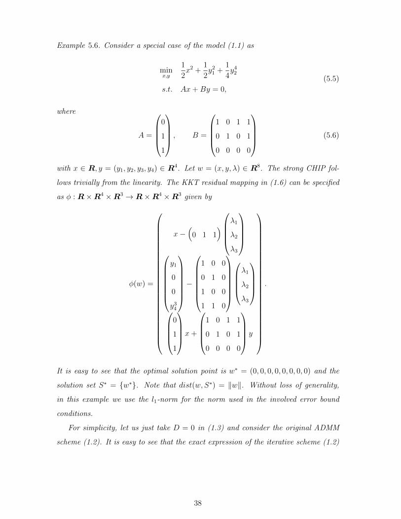
Example 5.6. Consider a special case of the model (1.1) as

minx,y

1

2x2 +

1

2y2

1 +1

4y4

2

s.t. Ax+By = 0,

(5.5)

where

A =

0

1

1

, B =

1 0 1 1

0 1 0 1

0 0 0 0

(5.6)

with x ∈ R, y = (y1, y2, y3, y4) ∈ R4. Let w = (x, y, λ) ∈ R8. The strong CHIP fol-

lows trivially from the linearity. The KKT residual mapping in (1.6) can be specified

as φ : R×R4 ×R3 → R×R4 ×R3 given by

φ(w) =

x−(

0 1 1)

λ1

λ2

λ3

y1

0

0

y34

−

1 0 0

0 1 0

1 0 0

1 1 0

λ1

λ2

λ3

0

1

1

x+

1 0 1 1

0 1 0 1

0 0 0 0

y

.

It is easy to see that the optimal solution point is w∗ = (0, 0, 0, 0, 0, 0, 0, 0) and the

solution set S∗ = w∗. Note that dist(w, S∗) = ‖w‖. Without loss of generality,

in this example we use the l1-norm for the norm used in the involved error bound

conditions.

For simplicity, let us just take D = 0 in (1.3) and consider the original ADMM

scheme (1.2). It is easy to see that the exact expression of the iterative scheme (1.2)

38

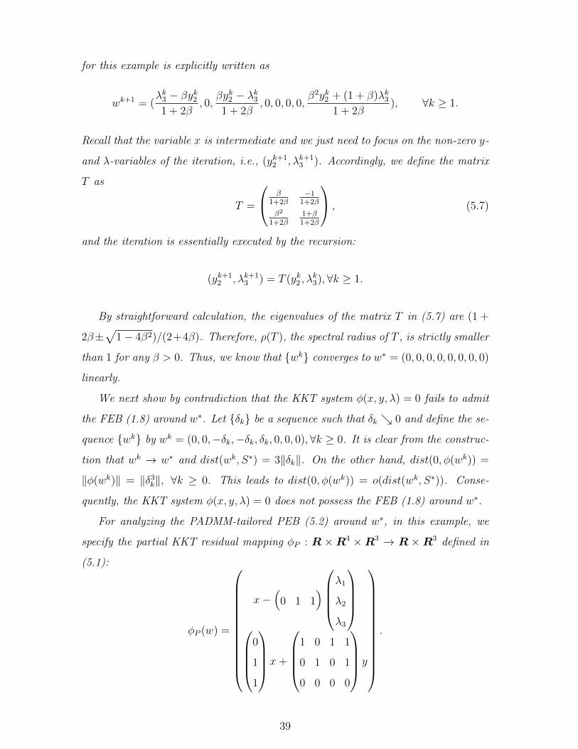
for this example is explicitly written as

wk+1 = (λk3 − βyk21 + 2β

, 0,βyk2 − λk31 + 2β

, 0, 0, 0, 0,β2yk2 + (1 + β)λk3

1 + 2β), ∀k ≥ 1.

Recall that the variable x is intermediate and we just need to focus on the non-zero y-

and λ-variables of the iteration, i.e., (yk+12 , λk+1

3 ). Accordingly, we define the matrix

T as

T =

β1+2β

−11+2β

β2

1+2β1+β1+2β

, (5.7)

and the iteration is essentially executed by the recursion:

(yk+12 , λk+1

3 ) = T (yk2 , λk3),∀k ≥ 1.

By straightforward calculation, the eigenvalues of the matrix T in (5.7) are (1 +

2β±√

1− 4β2)/(2+4β). Therefore, ρ(T ), the spectral radius of T , is strictly smaller

than 1 for any β > 0. Thus, we know that wk converges to w∗ = (0, 0, 0, 0, 0, 0, 0, 0)

linearly.

We next show by contradiction that the KKT system φ(x, y, λ) = 0 fails to admit

the FEB (1.8) around w∗. Let δk be a sequence such that δk 0 and define the se-

quence wk by wk = (0, 0,−δk,−δk, δk, 0, 0, 0),∀k ≥ 0. It is clear from the construc-

tion that wk → w∗ and dist(wk, S∗) = 3‖δk‖. On the other hand, dist(0, φ(wk)) =

‖φ(wk)‖ = ‖δ3k‖, ∀k ≥ 0. This leads to dist(0, φ(wk)) = o(dist(wk, S∗)). Conse-

quently, the KKT system φ(x, y, λ) = 0 does not possess the FEB (1.8) around w∗.

For analyzing the PADMM-tailored PEB (5.2) around w∗, in this example, we

specify the partial KKT residual mapping φP : R ×R4 ×R3 → R ×R3 defined in

(5.1):

φP (w) =

x−(

0 1 1)

λ1

λ2

λ3

0

1

1

x+

1 0 1 1

0 1 0 1

0 0 0 0

y

.

39

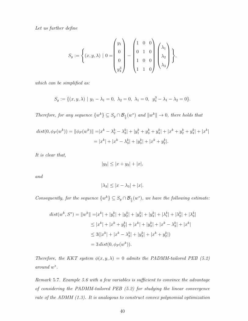
Let us further define

Sy :=

(x, y, λ) | 0 =

y1

0

0

y34

−

1 0 0

0 1 0

1 0 0

1 1 0

λ1

λ2

λ3

,

which can be simplified as:

Sy := (x, y, λ) | y1 − λ1 = 0, λ2 = 0, λ1 = 0, y34 − λ1 − λ2 = 0.

Therefore, for any sequence wk ⊆ Sy ∩ B 12(w∗) and ‖wk‖ → 0, there holds that

dist(0, φP (wk)) = ‖φP (wk)‖ =|xk − λk2 − λk3|+ |yk1 + yk3 + yk4 |+ |xk + yk2 + yk4 |+ |xk|

= |xk|+ |xk − λk3|+ |yk3 |+ |xk + yk2 |.

It is clear that,

|y2| ≤ |x+ y2|+ |x|,

and

|λ3| ≤ |x− λ3|+ |x|.

Consequently, for the sequence wk ⊆ Sy ∩ B 12(w∗), we have the following estimate:

dist(wk, S∗) = ‖wk‖ =|xk|+ |yk1 |+ |yk2 |+ |yk3 |+ |yk4 |+ |λk1|+ |λk2|+ |λk3|

≤ |xk|+ |xk + yk2 |+ |xk|+ |yk3 |+ |xk − λk3|+ |xk|

≤ 3(|xk|+ |xk − λk3|+ |yk3 |+ |xk + yk2 |)

= 3 dist(0, φP (wk)).

Therefore, the KKT system φ(x, y, λ) = 0 admits the PADMM-tailored PEB (5.2)

around w∗.

Remark 5.7. Example 5.6 with a few variables is sufficient to convince the advantage

of considering the PADMM-tailored PEB (5.2) for studying the linear convergence

rate of the ADMM (1.3). It is analogous to construct convex polynomial optimization

40

problems in higher dimension so that only the PADMM-tailored PEB (5.2) holds while

the FEB (1.8) does not.

Note that the matrix B given in (5.6) is not of full column rank; hence Assump-

tion 2.2 is not satisfied and this reflects that Assumption 2.2 is sufficient, instead of

necessary, to ensure the convergence of the PADMM (1.3). Moreover, it is verified

that the FEB (1.8) fails and thus it is invalid to explain the linear convergence rate of

the application of the ADMM (1.2) to this specific example. Instead, the PADMM-

tailored PEB (5.2) is satisfied for this example and hence the linear convergence rate

of the ADMM is theoretically explained.

41

Chapter 6

Difference of updating the primal

variables in ADMM (1.2)

Despite of the main purpose of studying the linear convergence rate of the PADMM

(1.3) under weaker error bound conditions, an interesting byproduct of this work is

a theoretical explanation for the difference of updating the primal variables x and y

in the iteration. For simplicity, let us just focus on the original ADMM (1.2) in this

chapter.

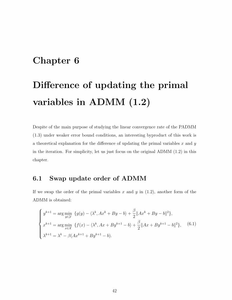
6.1 Swap update order of ADMM

If we swap the order of the primal variables x and y in (1.2), another form of the

ADMM is obtained:yk+1 = arg min

y∈Yg(y)− 〈λk, Axk +By − b〉+

β

2‖Axk +By − b‖2,

xk+1 = arg minx∈X

f(x)− 〈λk, Ax+Byk+1 − b〉+β

2‖Ax+Byk+1 − b‖2,

λk+1 = λk − β(Axk+1 +Byk+1 − b).

(6.1)

42

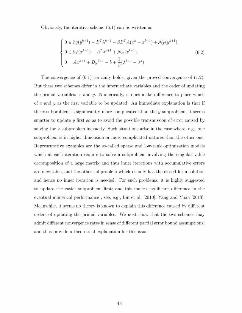
Obviously, the iterative scheme (6.1) can be written as

0 ∈ ∂g(yk+1)−BTλk+1 + βBTA(xk − xk+1) +NY(yk+1),

0 ∈ ∂f(xk+1)− ATλk+1 +NX (xk+1),

0 = Axk+1 +Byk+1 − b+1

β(λk+1 − λk).

(6.2)

The convergence of (6.1) certainly holds; given the proved convergence of (1.2).

But these two schemes differ in the intermediate variables and the order of updating

the primal variables: x and y. Numerically, it does make difference to place which

of x and y as the first variable to be updated. An immediate explanation is that if

the x-subproblem is significantly more complicated than the y-subproblem, it seems

smarter to update y first so as to avoid the possible transmission of error caused by

solving the x-subproblem inexactly. Such situations arise in the case where, e.g., one

subproblem is in higher dimension or more complicated natures than the other one.

Representative examples are the so-called sparse and low-rank optimization models

which at each iteration require to solve a subproblem involving the singular value

decomposition of a large matrix and thus inner iterations with accumulative errors

are inevitable, and the other subproblem which usually has the closed-form solution

and hence no inner iteration is needed. For such problems, it is highly suggested

to update the easier subproblem first; and this makes significant difference in the

eventual numerical performance , see, e.g., Lin et al. [2010]; Yang and Yuan [2013].

Meanwhile, it seems no theory is known to explain this difference caused by different

orders of updating the primal variables. We next show that the two schemes may

admit different convergence rates in sense of different partial error bound assumptions;

and thus provide a theoretical explanation for this issue.

43

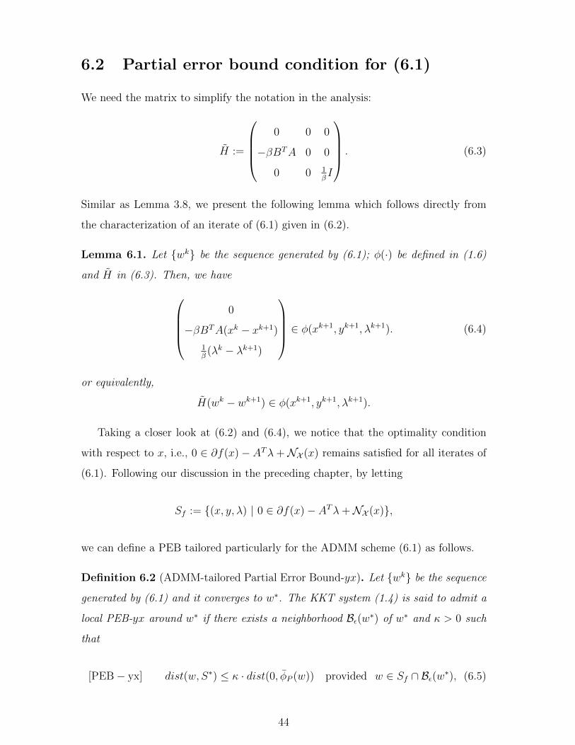
6.2 Partial error bound condition for (6.1)

We need the matrix to simplify the notation in the analysis:

H :=

0 0 0

−βBTA 0 0

0 0 1βI

. (6.3)

Similar as Lemma 3.8, we present the following lemma which follows directly from

the characterization of an iterate of (6.1) given in (6.2).

Lemma 6.1. Let wk be the sequence generated by (6.1); φ(·) be defined in (1.6)

and H in (6.3). Then, we have

0

−βBTA(xk − xk+1)

1β(λk − λk+1)

∈ φ(xk+1, yk+1, λk+1). (6.4)

or equivalently,

H(wk − wk+1) ∈ φ(xk+1, yk+1, λk+1).

Taking a closer look at (6.2) and (6.4), we notice that the optimality condition

with respect to x, i.e., 0 ∈ ∂f(x)− ATλ+NX (x) remains satisfied for all iterates of

(6.1). Following our discussion in the preceding chapter, by letting

Sf := (x, y, λ) | 0 ∈ ∂f(x)− ATλ+NX (x),

we can define a PEB tailored particularly for the ADMM scheme (6.1) as follows.

Definition 6.2 (ADMM-tailored Partial Error Bound-yx). Let wk be the sequence

generated by (6.1) and it converges to w∗. The KKT system (1.4) is said to admit a

local PEB-yx around w∗ if there exists a neighborhood Bε(w∗) of w∗ and κ > 0 such

that

[PEB− yx] dist(w, S∗) ≤ κ · dist(0, φP (w)) provided w ∈ Sf ∩ Bε(w∗), (6.5)

44

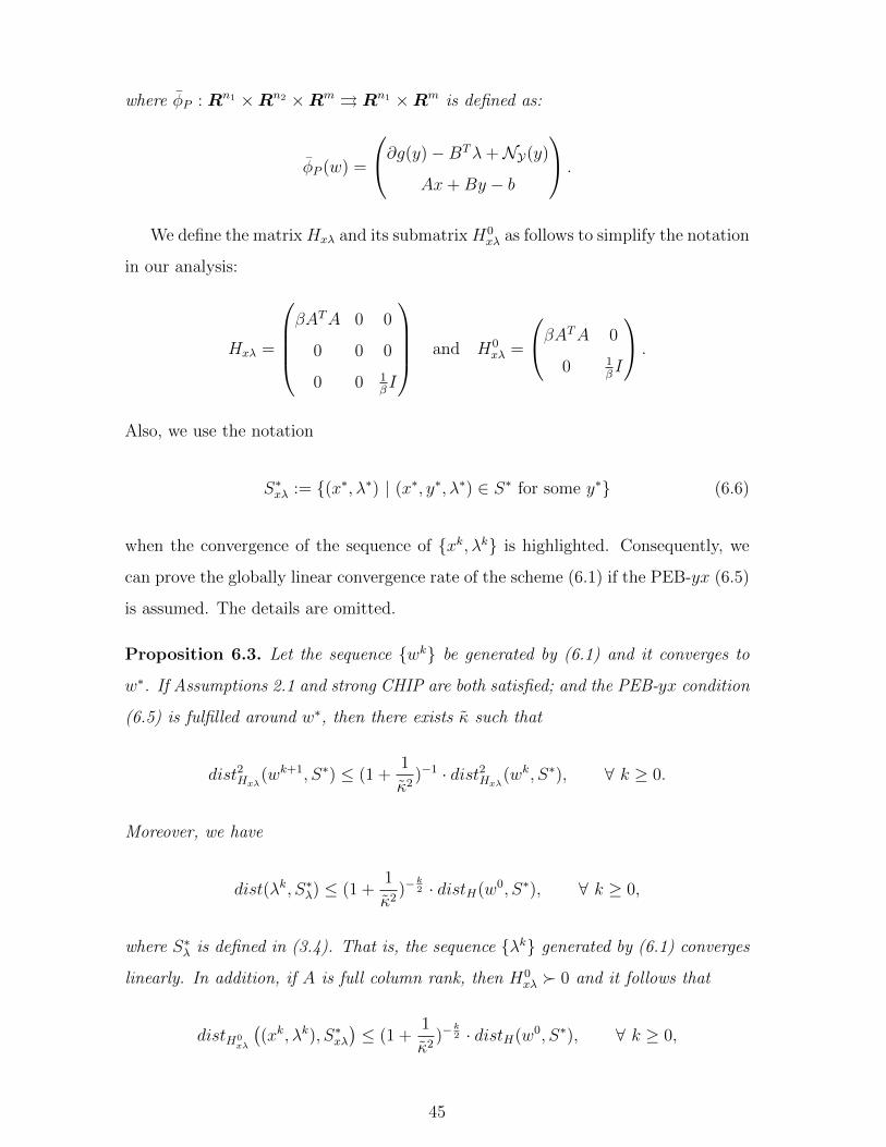
where φP : Rn1 ×Rn2 ×Rm ⇒ Rn1 ×Rm is defined as:

φP (w) =

∂g(y)−BTλ+NY(y)

Ax+By − b

.

We define the matrix Hxλ and its submatrix H0xλ as follows to simplify the notation

in our analysis:

Hxλ =

βATA 0 0

0 0 0

0 0 1βI

and H0xλ =

βATA 0

0 1βI

.

Also, we use the notation

S∗xλ := (x∗, λ∗) | (x∗, y∗, λ∗) ∈ S∗ for some y∗ (6.6)

when the convergence of the sequence of xk, λk is highlighted. Consequently, we

can prove the globally linear convergence rate of the scheme (6.1) if the PEB-yx (6.5)

is assumed. The details are omitted.

Proposition 6.3. Let the sequence wk be generated by (6.1) and it converges to

w∗. If Assumptions 2.1 and strong CHIP are both satisfied; and the PEB-yx condition

(6.5) is fulfilled around w∗, then there exists κ such that

dist2Hxλ(wk+1, S∗) ≤ (1 +1

κ2)−1 · dist2Hxλ(wk, S∗), ∀ k ≥ 0.

Moreover, we have

dist(λk, S∗λ) ≤ (1 +1

κ2)−

k2 · distH(w0, S∗), ∀ k ≥ 0,

where S∗λ is defined in (3.4). That is, the sequence λk generated by (6.1) converges

linearly. In addition, if A is full column rank, then H0xλ 0 and it follows that

distH0xλ

((xk, λk), S∗xλ

)≤ (1 +

1

κ2)−

k2 · distH(w0, S∗), ∀ k ≥ 0,

45

where S∗xλ is defined in (6.6). That is, the sequence (xk, λk) generated by (6.1)

converges linearly.

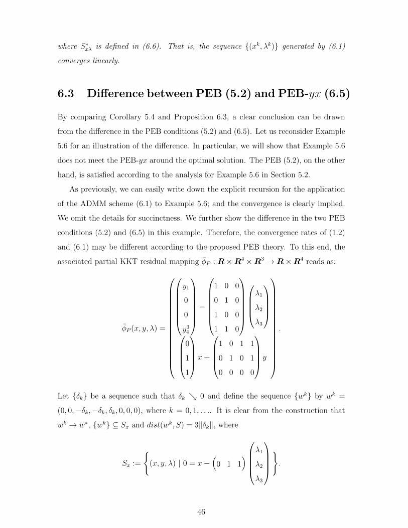
6.3 Difference between PEB (5.2) and PEB-yx (6.5)

By comparing Corollary 5.4 and Proposition 6.3, a clear conclusion can be drawn

from the difference in the PEB conditions (5.2) and (6.5). Let us reconsider Example

5.6 for an illustration of the difference. In particular, we will show that Example 5.6

does not meet the PEB-yx around the optimal solution. The PEB (5.2), on the other

hand, is satisfied according to the analysis for Example 5.6 in Section 5.2.

As previously, we can easily write down the explicit recursion for the application

of the ADMM scheme (6.1) to Example 5.6; and the convergence is clearly implied.

We omit the details for succinctness. We further show the difference in the two PEB

conditions (5.2) and (6.5) in this example. Therefore, the convergence rates of (1.2)

and (6.1) may be different according to the proposed PEB theory. To this end, the

associated partial KKT residual mapping φP : R×R4 ×R3 → R×R4 reads as:

φP (x, y, λ) =

y1

0

0

y34

−

1 0 0

0 1 0

1 0 0

1 1 0

λ1

λ2

λ3

0

1

1

x+

1 0 1 1

0 1 0 1

0 0 0 0

y

.

Let δk be a sequence such that δk 0 and define the sequence wk by wk =

(0, 0,−δk,−δk, δk, 0, 0, 0), where k = 0, 1, . . .. It is clear from the construction that

wk → w∗, wk ⊆ Sx and dist(wk, S) = 3‖δk‖, where

Sx :=

(x, y, λ) | 0 = x−

(0 1 1

)λ1

λ2

λ3

.

46

On the other hand, dist(0, φP (wk)) = ‖φP (wk)‖ = ‖δ3k‖ for k = 0, 1, . . .. This leads to

dist(0, φP (wk)) = o(dist(wk, S∗)). Consequently, the PEB-yx is not fulfilled around

w∗. That is, the ADMM (1.2) with the updating order of x− y admits the PEB and

it converges linearly, while the PEB-yx (6.5) is not satisfied and there is no guarantee

to the linear convergence rate for the ADMM (6.1) with the updating order of y− x.

47

Chapter 7

Discussion

We study error bound conditions to ensure the linear convergence rate for the al-

ternating direction method of multipliers (ADMM) in the convex programming con-

text. Different from existing literatures that requires stronger assumptions or special

structures on the model under discussion to sufficiently ensure certain error bound

conditions, we prompt weakening these error bound conditions by taking into con-

sideration the structures and properties of the specific algorithm under discussion.

That is, algorithmic-tailored error bound conditions should be considered and they

could be weaker than the generic-purpose error bound conditions. We give both full

and partial error bound conditions in accordance with the ADMM’s special iterative

scheme to derive its linear convergence rate; the idea of partial error bound is inspired

by an observation on the partially perturbed system (3.8). Furthermore, we construct

an example to show that the partial error bound condition is weaker than the generic

ones. The main analysis also inspires byproducts. First, a theoretical interpretation

is given to explain the difference if the two primal variable are updated by different

orders in ADMM’s iteration. Second, the equivalence among various error bound

conditions widely used in the literature is established. Our new philosophy of weak-

ening existing error bound conditions in accordance with the specific structure of an

algorithm under investigation may inspire other similar research in other contexts.

Moreover, we use the concepts of calmness/metric subregularity in our analysis, and

the main partial error bound result is inspired by a perturbation perspective. We

believe that more deliberated draw on the experience of these well-developed tech-

48

niques in variational analysis and perturbation analysis will lead to more interesting

and deeper results for the convergence analysis of other popular algorithms.

The linear convergence rates of ADMM schemes and other first-order methods

via various error bound conditions have been studied in other contexts as well. For

examples, in Hong and Luo [2017], an extended version of the ADMM scheme (1.2)

with a sufficiently small step size for updating the dual variable λ is considered for a

similar but more complicated case of (1.1) where there are more than two blocks of

functions in the objective; a variant of the PADMM is studied in Han et al. [to appear]

under calmness condition of Sprox−I defined in (4.2). In this paper, we concentrate

on the relatively simpler convex scenario where only the two-block separable convex

minimization model (1.1) and the proximal version of ADMM (1.3) are considered

so that our idea can be exposed with simplier notation more clearly. Technically, we

believe it is possible to extend our analysis to various more complicated scenarios such

as models with nonconvex function components in their objectives, more sophisticated

variants of the ADMM for two-block or even multiple-block models. Let us just

mention one specific extension: it is trivial to extend our analysis to a more general

version of the PADMM (1.3) considered in Eckstein and Bertsekas [1992]; Fang et al.

[2015]:

xk+1 = arg minx∈X

f(x)− (λk)T (Ax+Byk − b) +β

2‖Ax+Byk − b‖2 +

1

2‖x− xk‖2

D,

yk+1 = arg miny∈Yg(y)− (λk)T (Axk+1 +By − b)

+β

2‖αAxk+1 − (1− α)(Byk − b) +By − b‖2,

λk+1 = λk − β(αAxk+1 − (1− α)(Byk − b) +Byk+1 − b),

with α ∈ (0, 2) is a relaxation factor. We skip the tedious analysis for more compli-

cated extension and just present our analysis in the simplest context.

In the recent paper Drusvyatskiy and Lewis [2016], the authors investigate some

unconstrained separable convex optimization problems and illustrate that subregular-

ity of the gradient-like mapping is equivalent to the subregularity of its subdifferetial.

Therefore, they employ the quadratic growth condition as the characterization of the

error bound condition and establish the linear convergence rate for the proximal gra-

49

dient method. In the literature, there are many interesting works that provide char-

acterizations and criteria for error bound properties in terms of various derivative-like

objects in either the primal space (via directional derivatives, slopes, etc.) or the dual

space (via subdifferentials, normal cones). Notice that for a given w, the FEB (1.8)

around w is equivalent to the the metric subregularity of the KKT mapping φ at

(w, 0) and the calmness of S(p) at (0, w). The proximal EB-I (1.11) and proximal

EB-II (1.13) around w, on the other hand, are equivalent to the calmness of Sprox−I(p)

and Sprox−II(p) at (0, w), respectively. It is known that computing the exact formula

of those derivative-like objects is much simpler in absence of any proximal operators.

This perspective motivates us to call on existing extensive literature of the verifiable

first-order and second-order sufficient conditions for the metric subregularity of φ or

the calmness of S(p), see, e.g. Gfrerer [2011, 2013]; Gfrerer and Klatte [2016]; Gfrerer

and Mordukhovich [2015, 2017]; Gfrerer and Outrata [2016]; Gfrerer and Ye [2017];

Henrion et al. [2002]. Therefore, for the particular constrained model (1.1), we may

consider investigating verifiable sufficient conditions for the metric subregularity/-

calmness and hence the linear convergence rates for various ADMM-type algorithms

and other schemes. In particular, it is interesting to notice that for the problem data

with underlying polyhedral structures, the second-order sufficient condition is nearly

necessary, see, e.g. Gfrerer [2013]. This is our future work.

50

Bibliography

D. Boley. Local linear convergence of the alternating direction method of multipliers

on quadratic or linear programs. SIAM Journal on Optimization, 23(4):2183–2207,

2013.

S. Boyd, N. Parikh, E. Chu, B. Peleato, and J. Eckstein. Distributed optimization and

statistical learning via the alternating direction method of multipliers. Foundations

and Trends R© in Machine Learning, 3(1):1–122, 2011.

T. F. C. Chan and R. Glowinski. Finite element approximation and iterative solution

of a class of mildly non-linear elliptic equations. Computer Science Department,

Stanford University Stanford, 1978.

W. Deng and W. Yin. On the global and linear convergence of the generalized

alternating direction method of multipliers. Journal of Scientific Computing, 66

(3):889–916, 2016.

A. Dontchev and R. Rockafellar. Implicit Functions and Solution Mappings: A View

from Variational Analysis. Springer Series in Operations Research and Financial

Engineering. Springer New York, 2014. ISBN 9781493910373. URL https://

books.google.com.hk/books?id=LnAgBAAAQBAJ.

D. Drusvyatskiy and A. S. Lewis. Error bounds, quadratic growth, and linear con-

vergence of proximal methods. arXiv preprint arXiv:1602.06661, 2016.

J. Eckstein and D. P. Bertsekas. On the douglasrachford splitting method and the

proximal point algorithm for maximal monotone operators. Mathematical Pro-

gramming, 55(1):293–318, 1992.

51

J. Eckstein and W. Yao. Understanding the convergence of the alternating direction

method of multipliers: Theoretical and computational perspectives. Pac. J. Optim.,

11(4):619–644, 2015.

J. Eckstein, D. P. Bertsekas, et al. An alternating direction method for linear pro-

gramming. 1990.

F. Facchinei and J.-S. Pang. Finite-dimensional variational inequalities and comple-

mentarity problems. Springer Science & Business Media, 2007.

E. X. Fang, B. He, H. Liu, and X. Yuan. Generalized alternating direction method of

multipliers: new theoretical insights and applications. Mathematical programming

computation, 7(2):149–187, 2015.

M. Fortin and R. Glowinski. Augmented Lagrangian methods: applications to the

numerical solution of boundary-value problems, volume 15. Elsevier, 2000.

D. Gabay and B. Mercier. A dual algorithm for the solution of nonlinear varia-

tional problems via finite element approximation. Computers & Mathematics with

Applications, 2(1):17–40, 1976.

H. Gfrerer. First order and second order characterizations of metric subregularity

and calmness of constraint set mappings. SIAM Journal on Optimization, 21(4):

1439–1474, 2011.

H. Gfrerer. On directional metric regularity, subregularity and optimality conditions

for nonsmooth mathematical programs. Set-Valued and Variational Analysis, pages

1–26, 2013.

H. Gfrerer and D. Klatte. Lipschitz and holder stability of optimization problems

and generalized equations. Mathematical Programming, 158(1-2):35–75, 2016.

H. Gfrerer and B. S. Mordukhovich. Complete characterizations of tilt stability in

nonlinear programming under weakest qualification conditions. SIAM Journal on

Optimization, 25(4):2081–2119, 2015.

52

H. Gfrerer and B. S. Mordukhovich. Robinson stability of parametric constraint

systems via variational analysis. SIAM Journal on Optimization, 27(1):438–465,

2017.

H. Gfrerer and J. V. Outrata. On lipschitzian properties of implicit multifunctions.

SIAM Journal on Optimization, 26(4):2160–2189, 2016.

H. Gfrerer and J. J. Ye. New constraint qualifications for mathematical programs with

equilibrium constraints via variational analysis. SIAM Journal on Optimization,

27(2):842–865, 2017.

R. Glowinski. On alternating direction methods of multipliers: a historical perspec-

tive. In Modeling, simulation and optimization for science and technology, pages

59–82. Springer, 2014.

R. Glowinski and P. Le Tallec. Augmented Lagrangian and operator-splitting methods

in nonlinear mechanics. SIAM, 1989.

R. Glowinski and A. Marroco. Sur l’approximation, par elements finis d’ordre un, et

la resolution, par penalisation-dualite d’une classe de problemes de dirichlet non

lineaires. Revue franccaise d’automatique, informatique, recherche operationnelle.

Analyse numerique, 9(R2):41–76, 1975.

D. Han and X. Yuan. Local linear convergence of the alternating direction method

of multipliers for quadratic programs. SIAM Journal on numerical analysis, 51(6):

3446–3457, 2013.

D. Han, D. Sun, and L. Zhang. Linear rate convergence of the alternating direction

method of multipliers for convex composite quadratic and semi-definite program-

ming. Mathematics of Operations Research, to appear.

B. He and H. Yang. Some convergence properties of a method of multipliers for

linearly constrained monotone variational inequalities. Operations research letters,

23(3):151–161, 1998.

53

B. He and X. Yuan. On the o(1/n) convergence rate of the douglas–rachford alter-

nating direction method. SIAM Journal on Numerical Analysis, 50(2):700–709,

2012.

B. He and X. Yuan. On non-ergodic convergence rate of douglas–rachford alternating

direction method of multipliers. Numerische Mathematik, 130(3):567–577, 2015.

R. Henrion, A. Jourani, and J. Outrata. On the calmness of a class of multifunctions.

SIAM Journal on Optimization, 13(2):603–618, 2002.

M. Hong and Z.-Q. Luo. On the linear convergence of the alternating direction

method of multipliers. Mathematical Programming, 162(1-2):165–199, 2017.

Z. Lin, M. Chen, and Y. Ma. The augmented lagrange multiplier method for exact

recovery of corrupted low-rank matrices. arXiv preprint arXiv:1009.5055, 2010.

P.-L. Lions and B. Mercier. Splitting algorithms for the sum of two nonlinear opera-

tors. SIAM Journal on Numerical Analysis, 16(6):964–979, 1979.

G. Liu, J. Ye, and J. Zhu. Partial exact penalty for mathematical programs with

equilibrium constraints. Set-Valued Analysis, 16(5-6):785, 2008.

R. Liu, Z. Lin, and Z. Su. Linearized alternating direction method with parallel

splitting and adaptive penalty for separable convex programs in machine learning.

In Asian Conference on Machine Learning, pages 116–132, 2013.

Y. Liu, X. Yuan, S. Zeng, and J. Zhang. Weaker error bound conditions and linear

rate convergence of the alternating direction method of multipliers. Manuscript,

2017.

R. D. Monteiro and B. F. Svaiter. Iteration-complexity of block-decomposition al-

gorithms and the alternating direction method of multipliers. SIAM Journal on

Optimization, 23(1):475–507, 2013.

R. Nishihara, L. Lessard, B. Recht, A. Packard, and M. I. Jordan. A general analysis

of the convergence of admm. arXiv preprint arXiv:1502.02009, 2015.

54

S. M. Robinson. Strongly regular generalized equations. Mathematics of Operations

Research, 5(1):43–62, 1980.

R. T. Rockafellar and R. J.-B. Wets. Variational analysis, volume 317. Springer

Science & Business Media, 2009.

M. Tao and X. Yuan. On the optimal linear convergence rate of a generalized proximal

point algorithm. Journal of Scientific Computing, to appear.

X. Wang and X. Yuan. The linearized alternating direction method of multipliers

for dantzig selector. SIAM Journal on Scientific Computing, 34(5):A2792–A2811,

2012.

X. Wang, J. Ye, X. Yuan, S. Zeng, and J. Zhang. Linear convergence of the proximal

gradient method for nonsmooth nonconvex optimization problems via variational

analysis. Manuscript, 2017.

J. Yang and X. Yuan. Linearized augmented lagrangian and alternating direction

methods for nuclear norm minimization. Mathematics of computation, 82(281):

301–329, 2013.

W. H. Yang and D. Han. Linear convergence of the alternating direction method of

multipliers for a class of convex optimization problems. SIAM Journal on Numer-

ical Analysis, 54(2):625–640, 2016.

J. Ye and X. Ye. Necessary optimality conditions for optimization problems with

variational inequality constraints. Mathematics of Operations Research, 22(4):977–

997, 1997.

X. Zhang, M. Burger, X. Bresson, and S. Osher. Bregmanized nonlocal regularization

for deconvolution and sparse reconstruction. SIAM Journal on Imaging Sciences,

3(3):253–276, 2010.

55

CURRICULUM VITAE

Academic qualifications of the thesis author, Mr. ZENG Shangzhi:

• Received the degree of Bachelor of Natural Sciences (Mathematics and AppliedMathematics) from Wuhan University, June 2015.

October 2017

56